rational decision making - readingsample

Rational Decision Making

Bearbeitet vonFranz Eisenführ, Martin Weber, Thomas Langer

1st Edition. 2010. Taschenbuch. xiv, 447 S. PaperbackISBN 978 3 642 02850 2

Format (B x L): 15,5 x 23,5 cmGewicht: 726 g

Weitere Fachgebiete > Philosophie, Wissenschaftstheorie, Informationswissenschaft >Forschungsmethodik, Wissenschaftliche Ausstattung > Entscheidungstheorie,

Sozialwahltheorie

Zu Inhaltsverzeichnis

schnell und portofrei erhältlich bei

Die Online-Fachbuchhandlung beck-shop.de ist spezialisiert auf Fachbücher, insbesondere Recht, Steuern und Wirtschaft.Im Sortiment finden Sie alle Medien (Bücher, Zeitschriften, CDs, eBooks, etc.) aller Verlage. Ergänzt wird das Programmdurch Services wie Neuerscheinungsdienst oder Zusammenstellungen von Büchern zu Sonderpreisen. Der Shop führt mehr

als 8 Millionen Produkte.

http://www.beck-shop.de/Eisenfuehr-Weber-Langer-Rational-Decision-Making/productview.aspx?product=725167&utm_source=pdf&utm_medium=clickthru_lp&utm_campaign=pdf_725167&campaign=pdf/725167

http://www.beck-shop.de/trefferliste.aspx?toc=8827



http://www.beck-shop.de/fachbuch/inhaltsverzeichnis/9783642028502_TOC_001.pdf

Chapter 2: Structuring the decision problem

2.0 Summary 1. The basic structure of a decision problem entails alternatives, uncertainties,

consequences of alternatives and uncertainties, as well as the objectives and preferences of the decision maker.

2. Important decisions on the relevant alternatives have to be made in ad-vance. They refer to such questions as: Should further alternatives be consi-dered or should a choice be made from the existing ones? Should the num-ber of existing alternatives be reduced by merging similar alternatives or increased by splitting existing alternatives into several variants? Should the options be designed as one-stage or multi-stage alternatives?

3. Other important preceding decisions relate to the modeling of uncertainties. Can the future be predicted sufficiently well to neglect uncertainties in gen-eral? If not, what are the relevant uncertainties that influence the outcomes of the decision problem? In how much detail or how general should the un-iverse of possible states be modeled?

4. Uncertainty is described by states or events to which probabilities are allo-cated. Probabilities have to obey certain rules: joint probabilities and condi-tional probabilities are relevant to combining uncertain events. These com-binations can be visualized by the use of event trees or cause trees.

5. If an alternative is chosen and uncertainty resolved, a certain consequence will be obtained in a deterministic fashion. It might be necessary to formu-late an effect model that determines the consequences.

6. When modeling the preferences, a preliminary decision has to be made on whether a single objective or several objectives should be considered. The relevant objectives have to be identified. In the case of uncertain expecta-tions, risk attitude has to be considered, and in case of consequences that occur at different points in time, it might be reasonable to model time prefe-rence.

7. Usually, it is not possible to model the different components of the decision problem independently of one another. The components influence each oth-er. The decision maker moves back and forth between the set of alterna-tives, the uncertainty structure and his model of preferences until he finish-es modeling the decision problem and derives the optimal decision.

8. Graphical forms of representation such as the influence diagram, the deci-sion matrix, and the decision tree are very useful tools. They force the deci-sion maker to clarify his conceptions and support him in communicating with and explaining the decision fundamentals to other people involved in the decision process.

F. Eisenführ et al., Rational Decision Making, 19DOI 10.1007/978-3-642-02851-9_2, © Springer-Verlag Berlin Heidelberg 2010

20 Chapter 2: Structuring the decision problem

2.1 The basic structure The basic assumption of prescriptive decision theory is that a complex decision problem can be solved more effectively by decomposing it into several compo-nents (separate aspects). Instead of dealing with the problem as a whole, the deci-sion maker analyzes the components and creates models of o-nents. Afterwards, the partial models are merged to generate an overall model of the decision situation. These components were already mentioned in Chapter 1:

1. The alternatives (synonymous: options, actions). The decision maker has a number of alternatives from which to choose;

2. The uncertainties. These are incidents or states of the world that have an in-fluence on the decision, but cannot be controlled at all or at least only par-tially by the decision maker. The decision maker can only form expecta-tions about the resolution of uncertainty;

3. The consequences of actions and uncertainties. By choosing an alternative and the resolution of uncertainty, the resulting consequence is determined. This does not necessarily mean that the result is immediately known. An

the decision variables and event variables; 4. The objectives and preferences of the decision maker. The decision maker

has different preferences with respect to the consequences, i.e. he usually prefers one outcome over another. If no objective that the decision maker considers relevant is affected by the decision, there is no serious decision problem to solve.

Modeling is by no means unique; the same problem situation can be depicted in multiple ways. The remainder of this chapter covers several aspects and tools of modeling. The later chapters go into more detail on several key components.

2.2 The modeling of alternatives

2.2.1 The problem of finding alternatives

In some cases, finding the relevant alternatives is no problem; they are given in a a.m. about the closure of the highway

because of fog can choose between the trains at 6:59 a.m. and 7:13 a.m.; there are no other alternatives if he wants to be on time for his meeting. The jury can dec-lare the defendant to be guilty or not guilty. The voter can mark one of the given alternatives in the voting booth or return a blank or invalid sheet.

In many other situations, acceptable alternatives are not known immediately; generating them may be a considerable part of the problem. This can be a search process, as for instance that for someone who wants to buy a used car in a metro-politan area. It can also be a creative process of generating alternatives, e.g. when looking at different ways of constructing a machine, when reflecting on design op-

The modeling of alternatives 21

tions for a flower garden or when developing alternatives for the formulation of bylaws.

While searching for alternatives or generating them the question arises of when the process should be stopped and the decision made. Sometimes, time and budget restrictions limit the further creation of alternatives. In other cases, the dis-advantages of delaying the decision or additional cost of searching for further al-ternatives have to be weighed against the chances of finding a better solution than those determined so far. An additional complication arises if alternatives that are available right now (e.g. job offers, flats, used cars) could become unavailable when further delaying the decision.

These decisions about continuing or terminating the search for alternatives are decisions on their own. Sometimes they are trivial, compared with the actual deci-sion problem and can be made without elaborate analyses. When looking for a used VW Golf, you can decide easily if you want to pick one from the available offers or if you would prefer to wait a week. In other cases, like combating an acute danger an oil tanker accident, a hostage-taking, an epidemic the choice between the available options might be less problematic than the decision to con-tinue searching in the hope of finding a better alternative.

The decision to continue searching must be based on objectives and expecta-tions, just like every other decision. Objectives are necessary in order to evaluate the quality of the available options and to gain an impression of which alternatives might be superior. Expectations concerning the number and quality of additional alternatives have to be formed, as well as expectations about the effort associated with the process.

Chapter 4 deals with the problem of systematically generating new alternatives and preselecting the most appropriate ones.

2.2.2 The set of alternatives

The final decision entails the selection of one alternative from a given number of options. We define the set of alternatives as A and a single alternative as a; several alternatives are a, b, c etc.

As the name implies, alternatives must be mutually exclusive. It does not make TV in the even-

h-er, you obtain a set of mutually exclusive alternatives. Assume, for example, that

: a going out for lunch and watching TV in the evening, b going out for lunch and reading a book in the evening, c staying home for lunch and watching TV in the evening, d staying home for lunch and reading a book in the evening.

The set of alternatives A contains at least two elements. If the number of alterna-tives is so large that they cannot all be checked with the same intensity e.g. hun-


dreds of job applications for one open position pre-selection strategies have to be applied (see Chapter 4). One possible approach is to specify minimum re-quirements for the education and/or age of the applicants.

The number of alternatives is infinite for continuous decision variables. The possible amounts of money that can be spent on an advertising campaign can vary infinitely. The same holds for the production output of a detergent or the time in-vested by an expert in a particular project. Usually, it is possible to discretize a continuous variable without distorting the problem too much. As an example, an investor could choose a virtually infinite number of percentage values when split-ting his portfolio between bonds and stocks, but he can also reduce the endless number of alternatives to the following restricted set:

a 100% bonds, b 75% bonds, 25% stocks, c 50% bonds, 50% stocks, d 25% bonds, 75% stocks, e 100% stocks.

In this manner, we obtain a simplification of the decision problem, but simulta-neously also a coarsening. Assume the decision maker thinks that, of the given al-ternatives, the allocation of 75% to bonds and 25% to shares is optimal. If he thinks the set of alternatives is too coarse, he can fine-tune in a second step by choosing from similar alternatives such as 70, 75 and 80% bonds. In this book, we will mostly focus on situations in which only a few alternatives are considered.

2.2.3 One-level and multi-level alternatives

Every single decision is a part of the universe of decisions an individual has to make. This also applies to the time dimension: you only look ahead to a certain

u-ture decisions. Quite often it is foreseeable, however, what uncertainties are rele-vant for the future and how the decision maker could and should react to these events. No sophisticated chess player will think ahead only one step. Multi-level alternatives are also called strategies.1 A strategy is a sequence of contingent deci-sions; examples of two-level strategies are:

I will listen to the weather forecast and traffic report at 6 a.m. If both are encouraging, I will drive to work at 7:15 a.m., otherwise I will take the train at 6:59 a.m.

An additional amount of will be invested into the development project. If a marketable product exists by the end of the year, it will be pro-duced. If there is no marketable product, but further development looks promising, a well-funded associate should be sought to provide financial support. If the development is not promising, it should be terminated.

1 -level decisions are also included as a special case. Nevertheless, in everyday language, it is rather uncommon to use the term

-level decisions.

Modeling the states of the world 23

The choice of the number of decision levels that are taken into consideration is a preceding decision and similar to the issue of a further search for alternatives.

2.3 Modeling the states of the world

2.3.1 Uncertainty and probability

In a decision under certainty, every alternative is determined by an immediate consequence; no unknown influences affect it. In the case of uncertainty syn-onymously, we will also speak of risk in the following the outcomes depend on forces that cannot be fully controlled by the decision maker.2 Strictly speaking, there is no decision under total certainty. Anyone could be struck by a meteorite at any time or with a greater probability suffer a stroke. It is a subjective preced-ing decision to neglect or to consider the different sources of uncertainty. Fully neglecting uncertainty simplifies the problem in general, because only one state of the world has to be dealt with.

The reason why the uncertainty can be neglected is usually not that it is insigni-ficant; however, it is not necessary to account for uncertainty in the calculations if it is foreseeable that one alternative will turn out to be optimal for all scenarios. The optimal solution is independent of uncertain events, for instance, if the deci-sion can easily be reversed. If a decision is irreversible or can only be reversed at large cost, the risk has to be considered in the calculation. In many situations, un-certainty is the key problem; this is often the case for large investments, medical treatments, court decisions and political decisions of the legislature.

If you decide to consider uncertainty, it has to be formalized in a model which includes one or several uncertain facts (also known as chance occurrences). An uncertain fact is a set of outcomes, of which exactly one will occur. The set of out-comes is exhaustive and mutually exclusive, e.g. the outcome of a soccer game be-tween the teams A and B can be described by the set {A wins, B wins, A and B draw}.

The outcomes will occur either as events or as states. The result of a football game and the resignation of a CEO can be regarded as events, whereas the pres-ence of crude oil in a certain geological formation or the health status of a patient can be regarded as states. The distinction between states and events is irrelevant from a formal perspective.

2 A word of warning might be appropriate here. The use of terms in the literature is not very con-sistent in the domain of risk and uncertainty. Often, uncertainty is used as a general term to sub-

o-

We depart from these definitions because we think that the concept of ignorance is evasive and theoretically dubious (see also Section 10.1). Nevertheless, in the case of risk, the beliefs of the decision maker concerning the probability distribution can be more or less incomplete. The lit-erature often (see also the discussion on ambiguity aversion in Section 13).


Event and state variables are intrinsically discrete or continuous. The number of marriages on a specific day in a specific registry office, for instance, would be a discrete variable. The amount of rainfall, on the contrary, would be a continuous variable: in principle, there is an infinite number of possible amounts of rainfall for each single recording. However, how to treat an uncertain fact in the modeling of a decision situation is a question of expedience. In the same spirit as in our ear-lier discussion about decision variables, in many cases it makes sense to discretize a continuous chance variable. For example, for a very large investment decision it might be sufficient to vary the uncertain acquisition costs only in millions of dol-lars.

Table 2-1: Some uncertain states and events

Uncertainties States or events What will the weather be like tomorrow? dry

rainy

What will the dollar exchange rate in Frankfurt/Main be on Dec. 1, 2010?

Is Patient X infected with tuberculosis? Yes No

How will the union react to the

Accept Decline, but willing to negotiate Decline, strike ballot

Without loss of generality, we start by assuming a finite set of states. To each state si a probability p(si) is assigned. In order to qualify as a probability, the figures p(si) have to fulfill the following three conditions (Kolmogoroff 1933):

p(si) 0 for all i. p(si) = 1 (the certain state has the probability 1). p(si or sj) = p(si) + p(sj) (the probability of occurrence of one of several dis-

joint states equals the sum of the probabilities of the states).

2.3.2 Combined events or states (scenarios)

A decision situation is often best described by the combination of several uncer-tain facts. For example, in a decision problem, the quantity of US sales of a specif-ic product, as well as the dollar exchange rate, might be relevant. The setting is therefore described appropriately by combinations of sales figures and exchange rates.

of uncertainties have to be considered, they may stem, for instance, from the technic-al, economic, legal, social or political environment. In such cases, the modeling of


mber of relevant event or state sets can become overwhelmingly numerous. For four uncertain facts with three states each, there are already 34 = 81 scenarios to be considered. The proba-bility of each scenario cannot be determined by simply multiplying the probabili-ties of the states. This is possible only in the most often unrealistic case of inde-pendent events (see Section 2.3.3). The effort of defining and calculating probabilities for the scenarios has to be weighed against their usefulness. In par-ticular, in the context of strategic planning, scenarios form the basis of incorporat-ing uncertainty. It is desirable to have just a small number of distinct scenarios that can be used for evaluating risky strategic alternatives. A practical example that deals with the definition of such scenarios to model the world energy needs can be found in the case at the end of this chapter.

The combination of events can occur multiplicatively or additively. The first case is given if two or more events are intended to occur jointly. The second case is given if we are looking for the probability that out of multiple events, precisely one will occur

-in-law do tomorrow Each of these uncertain facts is described by an event set consisting of two events that are relevant to your decision:

What will the weather be like tomorrow? = {dry, rain} Will my mother-in-law visit us tomorrow? = {visit, not visit}.

You might be in

for both events happening jointly is derived by multiplying the probabilities of .

will rain tomorrow or your mother-in-sufficient here for one of the two events to occur. In such a case, the two relevant probabilities have to be combined in an additive manner.

In the following sections, both cases are discussed in more detail.

2.3.3 The multiplication rule

The concepts of conditional probabilities and joint probabilities are relevant to the conjunction of uncertain states. Let x be an event from the set of events X, and y be an event from the set of events Y. The conditional probability p(y x) is then the probability that y will occur, given that x has already occurred. This conditional probability is defined for p(x) > 0 as

p(y x) = p(x,y) / p(x). (2.1)

In this definition, p(x,y) refers to the joint probability of x and y. This is the probability that x and y will both occur.

From (2.1), it follows that

p(x,y) = p(x) p(y x). (2.2)


Eq. (2.2) is known as the multiplication rule and can be used to calculate the prob-ability of the joint occurrence of two events. Let us look at an example in order to explain these concepts. The uncertain fact X indicates the rate of economic growth of a country for the next three years. It is necessary to differentiate between three states: (x1) depression, (x2) stagnation, (x3) boom. Y stands for the results of the next general election; in this case, we only distinguish between the events (y1) vic-tory of the conservatives and (y2) victory of the socialists. Assume that the eco-nomic forecasts for the next years look like this:

p(x1) = 0.2 p(x2) = 0.65 p(x3) = 0.15.

The probabilities for the election outcome depend on the rate of economic growth.

The following conditional probabilities are formed:

p(y1|x1) = 0.4 p(y2|x1) = 0.6

p(y1|x2) = 0.5 p(y2|x2) = 0.5

p(y1|x3) = 0.6 p(y2|x3) = 0.4.

Using (2-2), this information allows us to calculate the joint probabilities which are listed in Table 2- l-

p(x3,y2) = p(x3) · p(y2|x3) = 0.15 · 0.4 = 0.06.

Table 2-2: Joint probabilities of economic growth and political development

Y (political development) p(xi) y1

(conservative) y2 (socialist)

X (economic growth)

x1 (depression) 0.20 0.08 0.12

x2 (stagnation) 0.65 0.325 0.325

x3 (boom) 0.15 0.09 0.06

sum 1 0.495 0.505

By summing over the joint probabilities in each row or column, the unconditional probabilities p(x) and p(y) of the two sets of events can be determined. They are also referred to as marginal probabilities. The marginal probabilities for economic growth were given; those for political developments are derived from the joint probabilities in the table; for instance, the conservatives will win with a probabili-ty of p(y1) = 0.495.

The calculation of joint probabilities can also be represented graphically. In Figure 2-1, each circle reflects a set of events that consists of several alternative events, depicted by the branches originating from the knots. The numbers are the probabilities assigned to these different possibilities of economic growth. Further to the right, the numbers reflect the conditional probabilities of the election result


depending on the economic growth and the resulting probabilities for the event combinations of economic and political development.

In the given example, the conditional probabilities p(y|x) differ, i.e. the proba-bility of a conservative or socialist victory in the elections is dependent on the rate of economic growth. A simpler situation would be given if all the conditional probabilities were the same; in this case, the unconditional probabilities would equal the marginal probability and the probability of a specific election outcome would in fact not be dependent on the economic development.

Independence Two events x and y are referred to as (stochastically) independent if for each yj the conditional probabilities p(yj|xi) are identical for each i and thus

p(y x) = p(y). (2.3)

Inserting this equation into (2.1), we obtain

p(x,y) = p(x) p(y), (2.4)

i.e. the joint probability of two independent events equals the product of their marginal probabilities.

2.3.4 Event trees

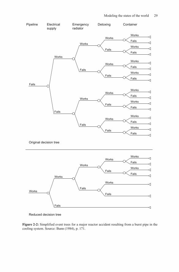
Event trees can be useful tools for depicting scenarios. An event tree starts with an uncertain fact that may lead to one of several possible events; each of these events can be followed by further events. The leaves of the tree (the triangles on the right) reflect event combinations (scenarios) that are mutually exclusive. Their probabilities can be calculated by multiplying the probabilities along the respec-tive path. With the exception of the probabilities at the root of the tree (i.e. the un-certain fact on the left), all the probabilities are conditional. Depending on the context, the expression state tree might be more appropriate than that of event tree.


0.2

0.15

Stagnation0.65

Boom

Depression

0.5

0.5

Conservative 0.325

Socialistic 0.325

0.4

0.6

Conservative 0.08

Socialistic 0.12

0.6

0.4

Conservative 0.09

Socialistic 0.06

Economic growth

Results of election

Figure 2-1: Event combinations and their probabilities derived by the multiplication rule

The graphical representation of the election scenario in Figure 2-1 is a very simple example of an event tree. As a further example, we consider the event tree that

s-sion from 1975 (the so-called Rasmussen report). It was generated to analyze the probabilities of serious reactor accidents. As can be seen in Figure 2-2, a major

; subsequently, the reaction of other parts of the sys-tem is considered. More explicitly, the internal power supply, the emergency cool-ing system, the disposal system for nuclear fission waste and the container system are modeled in detail. For each of these system components, only two events the system component works or fails are considered.

Every path through the event tree stands for the theoretical possibility of a se-quence of accidents. Not all the sequences are logically meaningful. If, for exam-ple, the electricity supply fails, none of the other system components can work. An event that occurs with probability zero and all the following events can be elimi-nated from the tree. Accordingly, the event tree can be simplified as shown in the lower part of Figure 2-2.


Works

Fails

Works

Fails

Works

Fails

Works

Fails

Works

Fails

Works

Fails

Works

Fails

Works

Fails

Works

Fails

Works

Fails

Works

Fails

Works

Fails

Fails

Works

Fails

Works

Fails

Works

Fails

Works

Fails

Works

Fails

Works

Fails

Works

Fails

Works

Fails

Works

Fails

Works

Reduced decision tree

Original decision tree

Pipeline Electrical supply

Emergency radiator

Detoxing Container

Figure 2-2: Simplified event trees for a major reactor accident resulting from a burst pipe in the cooling system. Source: Bunn (1984), p. 171.


2.3.5 The addition rule

The probability of either x or y or both occurring is

p(x or y) = p(x) + p(y) p(x,y). (2.5)

The subtractive term becomes clear if we realize that both p(x) and p(y) already include p(x,y); this term is therefore counted twice and has to be subtracted.

Assume, for instance, that a farmer estimates the probability of pest infestation to be p(x) = 0.2 and the probability of drought to be p(y) = 0.15. How high is the probability that the crop is destroyed if each of the two catastrophes can cause to-tal destruction? In order to make this calculation, we need the probability of the subtractive term p(x,y), i.e. the probability of pest infestation and drought occur-ring simultaneously. If infestation and drought are stochastically independent, this value is 0.2 · 0.15 = 0.03. The danger of crop loss is then 0.2 + 0.15 0.03 = 0.32. However, it is also possible that there is stochastic dependence, such as a higher probability of infestation in the case of drought, compared with periods of humidi-ty. Assuming the farmer estimates the (conditional) probability of infestation in the case of drought to be 1/3, we then obtain p(x,y) = 0.15 · 1/3 = 0.05 and the danger of losing the crop is 0.2 + 0.15 0.05 = 0.3.

If x and y are mutually exclusive, i.e. they cannot happen at the same time, the subtractive term equals zero. If the pest does not survive a drought and the proba-bilities p(x) and p(y) stand as stated above, the probability of losing the crop is 0.2 + 0.15 = 0.35.

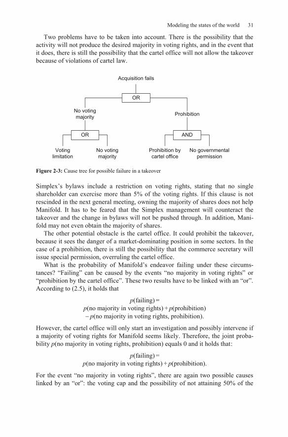
2.3.6 The cause tree

A second instrument that played a major role in the preparation of the earlier-mentioned reactor safety study is the fault tree, which reverses the idea of the event tree. The starting point is a predefined final result and the aim is to deter-mine how it could or did happen. As the name suggests, this method was con-structed for analyzing accidents reactor accidents, plane crashes, failures of au-tomobiles. Fault trees are suited to analyzing the causes of malfunctions of complex systems. Like an event tree, a fault tree is not restricted to unpleasant or negative events, which is why we prefer to use .

A cause tree starts with the effect and attempts to determine the possible caus-es. For each cause, it then continues to consider what could have induced it.

In event trees, we only observe multiplicati -conjunctions) between events, i.e. the joint occurrence of several events. In cause

-conjunctions, which require the addition of probabilities.

The mode of operation of a cause tree is depicted in the example in Figure 2-3. The Manifold corporation owns 20% of the shares of Simplex corporation, which competes in the same markets. The management of Manifold is interested in a ma-jority holding. As the Simplex shares are widely spread, but not traded on an ex-change, the management is considering a public takeover bid and offering the Simplex shareholders an attractive price for their shares.


Two problems have to be taken into account. There is the possibility that the activity will not produce the desired majority in voting rights, and in the event that it does, there is still the possibility that the cartel office will not allow the takeover because of violations of cartel law.

Acquisition fails

OR

ProhibitionNo votingmajority

OR AND

No governmental permission

Prohibition by cartel office

No voting majority

Votinglimitation

Figure 2-3: Cause tree for possible failure in a takeover

clude a restriction on voting rights, stating that no single shareholder can exercise more than 5% of the voting rights. If this clause is not rescinded in the next general meeting, owning the majority of shares does not help Manifold. It has to be feared that the Simplex management will counteract the takeover and the change in bylaws will not be pushed through. In addition, Mani-fold may not even obtain the majority of shares.

The other potential obstacle is the cartel office. It could prohibit the takeover, because it sees the danger of a market-dominating position in some sectors. In the case of a prohibition, there is still the possibility that the commerce secretary will issue special permission, overruling the cartel office.

What is the probability of endeavor failing under these circums-

iAccording to (2.5), it holds that

p(failing) = p(no majority in voting rights) + p(prohibition)

p(no majority in voting rights, prohibition).

However, the cartel office will only start an investigation and possibly intervene if a majority of voting rights for Manifold seems likely. Therefore, the joint proba-bility p(no majority in voting rights, prohibition) equals 0 and it holds that:

p(failing) = p(no majority in voting rights) + p(prohibition).

the voting cap and the possibility of not attaining 50% of the


shares. The probability of an overall failure because of a failure to obtain a majori-ty in voting rights may be decomposed as follows:

p(no majority in voting rights) = p(voting cap) + p(no majority of shares)

p(voting cap, no majority of shares).

We will next look at the probability of the prohibition. For this to happen, the car-tel office has to forbid the takeover and the commerce secretary has to refuse to issue special permission. The probability of this scenario equals the product of the probabilities of the cartel office forbidding the takeover and the (conditional) probability that, given a prohibition by the cartel office, the secretary will not overrule the prohibition and will deny a special permission:

p(prohibition) = p(cartel office forbids) p(secretary does not overrule cartel office forbids).

2.3.7 The dependence of the uncertainty model on the objectives

Unquestionably, there is an endless number of ways to model the uncertain envi-ronment. The decision as to which of the uncertain facts the decision maker takes into account and with which sets of states he chooses to model the uncertainty should be primarily influenced by his objectives.

Consider two men who are both thinking of buying a certain piece of land. Their decision is influenced by uncertainty. One of the potential buyers is a farmer who wants to grow tomatoes on the land. For him, the success of the decision de-pends on whether competitors will settle in the same area, whether import relief for foreign tomatoes can be expected and whether the use of insecticides will be restricted by law. He defines scenarios as combinations of different levels of com-petition, trade regulations and environmental laws and tries to determine proba-bilities of these scenarios arising.

The other potential buyer plans to build a fun park on the land and to exploit it commercially. He is obviously not interested in any of the uncertainties the farmer worries about; instead, he cares about other uncertainties like the population de-velopment in the area, the costs of construction and maintenance and possible sub-sidies by the municipality. The scenarios he considers are totally different from those of the farmer.

This example highlights the fact that objectives play a key role in the modeling process. We discussed this aspect before when looking at the process of generat-ing new alternatives. Not only the compilation of the set of alternatives, but also the choice of relevant events and states, must be guided by objectives. If the deci-sion maker does not (yet) know what he wants to achieve, he cannot identify the relevant uncertain states.

The modeling of preferences 33

2.4 The modeling of consequences If one alternative was chosen and specific states realized (i.e. the relevant uncer-tainties have been resolved), we assume the occurrence of a unique consequence.

. The consequence is not always that easy to determine. It might be necessary to

use an impact model that uniquely defines the consequence of the decision. A trad nings before taxes from an export deal PT are given by a function of the selling price s, the quantity of sales (depending on p) q, the pur-chase price k, the tax rate t and the exchange rate x. The decision alternatives are the different selling prices. The other variables are uncertain figures. The equation

PT = (1 t) q(s) (p x k)

is the model that defines the consequence PT by combining the decision variable (s) and the state variables (q, k, t, x).

The model can consist of one equation or a system of equations, but it can also be a complicated algorithm. Take as an example a production division in which many customer orders wait to be processed. For each order, what is known is which machines are needed, how long the order will take, in what sequence the order occupies the machines and for which date the delivery is planned. In the case where several orders wait in line for a specific machine, i.e. more than one order is ready to be processed by a machine, a priority rule can be used. Examples of

closest problem is which priority rule to establish. As soon as a new rule is introduced, a totally different sequence plan is scheduled. This does not mean that the plan is al-ready known; it has to be determined first. In order to accomplish this goal, a spe-cial algorithm is used that determines, usually software-supported, when to start which order, when to process it with which machine and when which order is completed. Only by the application of this algorithm does the impact of the chosen alternative on the objective variable become known.

2.5 The modeling of preferences

2.5.1 Objectives and preferences

to their consequences. We distinguish between the following relations for a, b A:

a b a is preferred to b. a ~ b indifference between a and b. a b a is preferred to b or there is indifference.


The preferences regarding the alternatives are not given beforehand; the decision maker usually has no coherent perception of them. It is the aim of decision analy-sis to support the decision maker in deriving them. To arrive at this point, it is im-

d-ing the consequences that result from states or events of relevant uncertainties and from choosing a particular alternative.

In a first step, the decision maker has to figure out which aspects of the conse-quences have an impact on his preferences and are therefore relevant for him when solving the decision problem. Before buying a car, he could realize that re-liability and costs are two aspects overall eco-balance, the sum of environmental effects during production, usage and disposal, does not matter to him. Combined with a statement about the direc-tion of his preference, the decision maker hereby identifies his objectives. In this

a-charac-

teristics he wants to use to describe explicitly the relevant consequences of his de-cision. These characteristics are also called attributes, objective variables or target variables. In the case of buying a car, he could describe the reliability in terms of the frequency of breakdowns, which he wants to minimize. The cost objective could be operationalized by a suitable combination of purchase price and running expenses. In the above-mentioned problem regarding the sequential processing of orders, attributes, such as mean pass-through time, number of missed deadlines or mean machine utilization could be chosen.

The level of valuation of an objective variable often decreases or increases mo-notonically with the value of the objective variable: lower costs and higher relia-bility are always better. In other cases, the optimal values are somewhere in the middle of the range. A person on vacation is interested in warm weather, but not the maximum possible heat; a surfer needs wind but not a hurricane. In these cas-

.

2.5.2 Conflict of objectives

One of the precedent decisions is to specify by how many and by which characte-ristics the consequences are defined. Chapter 3 will deal with this problem. In many economic decisions, one can concentrate on a single objective variable, like

various objectives exist that conflict with each other. The conflict is that there is no alternative that is better or at least not worse with respect to any objective variable; you cannot have everything. Solving the conflict always requires making trade-offs. The tran-sition from alternative a to alternative b might cause an improvement for some ob-jectives but a deterioration for other objectives at the same time.

In the following discussion, we will assume in most cases that the total value of a consequence for a decision maker results from the simple aggregation of the evaluations for the various relevant characteristics. We know this principle from

The modeling of preferences 35

many practical applications such as product tests, sports (e.g. decathlons) or ana-lytical performance evaluations. In all these cases, the importance of the different aspects is accounted for by using weights or point schemes. In decision analysis, the use of an additive aggregation model is quite common. In contrast to the most-ly naïve application of such concepts in practice, decision analysis clearly pre-scribes under what circumstances an additive model is acceptable and how to pro-

preferences. We will discuss these questions in more detail in Chapters 5 and 6.

2.5.3 Risk preferences

In the case of decisions under uncertaintyrisk plays an important role. In decisions under certainty, the problem is restricted to choosing between (certain) consequences a problem that can be challenging enough if there are conflicting objectives. The best consequence determines the best alternative. In the case of uncertainty, one has to choose between alternatives that can lead to different consequences. Each alternative is represented as a bundle of possible consequences, each occurring with some probability. In the literature,

an investment which has a low but cer-tain return, and engaging in some speculative investment transactions, e.g. buying some high-risk securities, a risk-averse investor might choose the first while a risk-seeking investor prefers the latter. Neither of them could be labeled as acting irrationally, however. Decision analysis explains how to measure subjective risk attitude and how to make complex decisions under uncertainty considering this individual risk attitude. We will deal with these issues in Chapters 9 and 10.

2.5.4 Time preferences

The implications of a decision are often spread out over a considerable period of time, one could say that a decision has several consequences distributed over time. Individuals are usually not indifferent between the temporal spreading of conse-quences over time instead, they have time preferences. People tend to postpone unpleasant surgery, for example, but they prefer to go on a cruise this year rather than next year. The decision about the correct point in time to start the retirement savings process is a typical question of time preference. It is a trade-off between consuming today and the perspective of having consumption opportunities in old age. In order to evaluate consequences that are spread widely over time, it is ne-cessary to model time preferences. This problem will be discussed in Chapter 11.

2.5.5 Modeling preferences by functions

by functions. These functions assign evaluations to the consequences or outcomes, in order to reflect the preference. In the case of certain expectations, the prefe-rence functions are called value functions; under risk, they are called utility func-


tions. These functions are derived from preference statements in very simple choice problems or at least from problems that are much easier to solve than the decision problem we are interested in. If the decision maker is able to give consis-tent answers, a value function or a utility function can be derived. This derivation is based on axioms that are commonly accepted as principles of rational behavior. The function can then be used to evaluate more complex alternatives.

In contrast to many criteria that are suggested in theory and practice and are more or less arbitrarily-defined decision rules, the procedures and concepts of de-cision analysis have the advantages that

the evaluation of alternatives is founded axiomatically, i.e. if the decision

maker accepts a few basic rationality postulates, the evaluation and optimal decision follows logically and unequivocally.

2.6 Recursive modeling The basic principle of decomposing a complex problem into modules that can be handled more easily separately does not mean that these modules are independent of one another. It is almost never possible to model alternatives, uncertainties and objectives completely separately from one another. We have already pointed out the superordinate function of objectives several times in the last few sections.

Figure 2-4 symbolizes how these components influence one another. Because of these influences, it is not possible to generate the sub-models in a single linear run. Instead, a change in one of the sub-models can also cause the need for a revi-sion of another sub-model. The decision maker thus goes back and forth repeated-ly between the different sub-models in order to adjust them to one another opti-mally. We call this process recursive modeling and will illustrate this procedure by means of the following example.

Objectives and preferences

AlternativesEnvironmental

influences Figure 2-4: Mutual impact of the sub-models

Let us assume you are considering purchasing a notebook to replace the desktop PC that you have been using at home so far. You talk to a friend who owns a

tisfied with it. After this conversation, your deci-sion situation can be described as follows:

Recursive modeling 37

1. Alternatives: I gain a better overview of the market situation first or I decide not to purchase a notebook for now.

2. Uncertainties: How quickly will a model that I buy today be outdated and unable to

work with modern software? Will low-budget models frequently cause problems that require money

and time to resolve? To what extent will I need the notebook in the near future for work that I

could not simply do at home at my desk?

3. Objectives: The notebook should be as low cost as possible. It should be as powerful as possible. It should be as easy to handle as possible. I would also like to be able to use the notebook on campus, in particular,

when researching literature in the library, so I do not need to transcribe my scribbling later at home.

After this first modeling of the situation, you turn to computer shops for advice and study relevant magazines.

Alternatives Objectives: You come to know more and more models, and since these have different characteristics which spark your interest, you develop new objectives. For instance, you realize that there are pleasant and less pleasant keyboards and that especially weight, display size and battery longevity vary con-siderably. Thus, the enhancement of the set of alternatives causes an enlargement of the system of objectives.

Objectives Alternatives: However, the inverse effect occurs as well. The longer your wish list becomes, the higher your motivation to search for better al-ternatives. New opportunities occur; others are dismissed you almost bought in the beginning, might not even be a serious option any long-er. In addition, you enlarge your set of alternatives by not only taking classic note-book models into consideration. Instead, you now also think about buying a sub-notebook that could be used in combination with the desktop at home.

Uncertainties Objectives: You think about how quickly the notebook will be outdated and will have problems with modern, memory-intensive applications. You realize that it is very important for you that you can still use the notebook for your final thesis in two years. This objective, which will probably eliminate the option of buying an older model, was not part of your explicit set of objectives be-fore.

Objectives Uncertainties: It is one of your objectives to keep costs as low as possible. Therefore, you make an effort to collect information on how prices of notebooks will probably develop during the upcoming year and whether larger


price jumps can be expected. It also matters to you what technological improve-ments can be expected in the near future.

Alternatives Uncertainties: By chance, you run into a bargain offer. A note-book that has hardly been used and is in a performance class far above the one you were originally interested in is offered to you at a discount of 40% compared to its original price. It still costs more than you intended to spend. The bargain offer would only pay off if you also needed the notebook for modern computer games with special graphics requirements. Due to your challenging field of study, it seems questionable whether you will have any time at all during the upcoming years to play computer games.

Uncertainties Alternatives: Contemplating the intensity of notebook usage that can be expected, you realize that you often need to print out (multicolored) slides for some lectures in order to make notes during class. You realize that if you bought a tablet PC instead of a regular notebook, you could insert your comments directly into the electronic slides and not only save considerable printing costs, but also help save the environment. You now also take this alternative into considera-tion seriously.

At some point in time, you have to push yourself to make a decision. The mod-eling of alternative actions, uncertain facts, objectives and preferences has to be terminated at some point. Based on the resulting model of the decision problem, you make a decision. This decision could also be to refrain from buying a note-book at all for the time being.

2.7 Visualization of decision situations under uncertainty

2.7.1 Benefits of graphical representations

Structuring and modeling a decision problem aims to support the decision maker in better understanding the problem and increasing the rationality of the solution. The means of representation we will discuss in the following support this goal. They force the decision maker to be clear and precise in phrasing objectives, alter-natives, influences and consequences. In addition, they allow the decision maker to convey his perspective of the problem to other people in a clearer and less am-biguous way than would be possible with a purely verbal description.

The three types of graphical representation that we will discuss below the in-fluence diagram, decision matrix, and the decision tree play different roles in the decision process. The influence diagram aims to provide a comprehensive impres-sion of the general structure of the decision problem. It provides an overview of the interaction of the problem constituents (decision components, uncertainties, objectives) that are considered to be relevant. Such an overview is important to understanding whether sub-problems can be separated and addressed in isolation, and at what stage of the decision process what information has to be available. To ensure clarity, most details are kept out of an influence diagram. In particular, it is not explicitly displayed which alternatives are under consideration and what spe-

Visualization of decision situations under uncertainty 39

cific uncertainty scenarios are regarded. To deal with such details, decision ma-trices and decision trees will be employed in a later stage of the decision process. The two types of graphical representation are very similar with respect to their in-formational content (and we will discuss this issue further in Section 2.7.5). They both display full information about alternatives, uncertain events and conse-quences (and thereby of course also information about the objectives of the deci-sion maker). In particular, the decision matrix arranges and presents the relevant data in a way that most easily allows us subsequently to derive a numerical solu-tion.

2.7.2 The influence diagram

Influence diagrams (Howard and Matheson 1984, Oliver and Smith 1990) play an important role in the problem structuring phase, i.e. in an early stage of the deci-sion analysis process. The great relevance of this tool can be illustrated by the fact

-based presenta i-sion Analysis (Horvitz 2005) contains mostly articles that deal with influence dia-grams. The survey article by Howard and Matheson (2005) that appeared in this special issue is by far the most frequently cited article that ever appeared in Deci-sion Analysis.

Influence diagrams do not display all possible actions but only the decisions per se. The set of alternatives is represented by a single symbol (rectangle) that does not convey how many and which alternatives exist. Likewise, not each single event but only the overall set of events is represented by a circle or an oval. Addi-tionally, the single consequences do not appear but only the objective variables, symbolized by diamonds or hexagons.

When decision D2 is due to be made it is knownwhich alternative has been chosen at decision D1.D1

T

X

X

D2

D

D

X Y

D

X T

When decision D is due to be made it is knownwhich event occurred from the set of events X.

The probabilities of the occurrences of the set Xdepend on decision D.

The probabilities of the occurrences of the set Ydepend on the event which occurs fromthe set of events X.

The specification of the target variable T dependson the chosen alternative at decision D.

The specification of the target variable T dependson the event which occurs from set X.

Figure 2-5: The presentation of relations in an influence diagram


Arrows pointing to a decision symbol depict a piece of information available at the time of the decision. Arrows pointing to an event symbol mean that the event probabilities depend on the directly preceding event or the directly preceding deci-sion.

If two event symbols are connected by an arrow, this indicates stochastic de-pendence between them, but does not necessarily have to indicate causality. In principle, the direction of an arrow could just as well be reversed, because if X is stochastically dependent on Y then also Y is stochastically dependent on X. If an arrow is missing, the events are independent of each other.

Figure 2-5 summarizes the most important constellations. Cycles are not per-mitted, i.e. there must not be a path through the diagram with identical starting and end points.

Let us begin with a simple case: a manufacturer of car accessories has devel-oped a new anti-theft device. The question arises of how large a production capac-ity should be chosen. In order to forecast the sales potential, the decision has been made to offer the product in a local market for a few months. The price has al-ready been determined and the costs are known. Depending on the sales in the test market, the probability distribution for the countrywide demand can be predicted and a decision about the production capacity can be made. Profit is the only objec-tive variable to be considered. Figure 2-6 shows a suitable influence diagram for this problem.

1

Capacity

Sales ontest market

Countrywide demand

Profit

32

4

Figure 2-6: concerning production capacity

Let us take a closer look and begin with the sales volume in the test market, which is still uncertain at the present time. When this figure becomes known, the coun-trywide demand can be assessed (arrow 1). This can refer to both a deterministic forecast and a probability distribution for the countrywide demand. Arrow 2 indi-cates that sales in the test market are known before the decision on the capacity is made. Arrows 3 and 4 depict that the profit is influenced by both the countrywide demand and the chosen production capacity.

In this example, you can see that the direction of the arrow between the two e-

versed, which would represent the true causality. However, from the decision as it is consis-


tent with the chronological order: first, sales in the test market are known, then the assessment of countrywide demand results.

Let us consider a somewhat more complicated case that is based on a study by Jensen et al. (1989). It deals with the decision of a US state whether or not to re-quire the use of smoke detectors in residential buildings by law. Furthermore, if this decision is made in favor of the detectors, a decision has to be made on the

a-tion by law is able to reduce the number of casualties and injuries depends on nu-merous factors. The more home owners voluntarily install smoke detectors any-way, the smaller the effect. In addition, a certain refusal rate has to be taken into consideration; not everybody will adhere to the law. This can be influenced by the intensity of enforcement of the regulation, e.g. via inspections. Further influence factors obviously are the fire frequency and the failure rate of smoke detectors. In addition to the reduction in the number of human casualties, further goals of the measures are the reduction in financial damage and the minimization of private and public costs. The different influences are represented in Figure 2-7.

Firefrequency

Publicsectorcosts

Privatecosts

Deathtoll

Number ofinjured

Materialdamage

Triggeredalarms

Failurerate

Existing smoke detectors

Voluntaryuse

Refusalrate

Make smokedetectors

compulsory?Intensity of

enforcement?

Figure 2-7: Influence diagram for the decision on whether to regulate the use of smoke detectors

One of the strengths of influence diagrams is their assistance in structuring a prob-lem. A second strength is the ability to communicate and document the relevant decisions and uncertain influences in a well-arranged manner. Of course, the iden-tification of the influences is not sufficient to make a decision; in fact, in a second step, these influences have to be quantified in a model. In the previous example, for instance, it would be necessary to estimate on a statistical basis how the num-ber of human casualties and the magnitude of financial damage is related to the number of fire alarms triggered.


This detailed information is intentionally not integrated into the influence dia-gram, however; otherwise, the diagram could no longer serve its purpose of pro-viding a good overview of the general structure of the decision problem. Never-theless, even despite the lack of detail, influence diagrams can become very extensive for complex decision problems. An example is shown in Figure 2-8, de-picting influence factors on possible health effects 10,000 years after the closure of a nuclear waste disposal site. This excerpt of an influence diagram displays which uncertain factors might influence the objective variable in combination with the construction of the barrier system. Even though this presentation is no longer particularly clear, it is definitely better suited to formulating and documenting views of complex interactions in a collaboration of experts than is purely verbal explanations.

Afterwards, the decision alternatives as well as the relevant uncertainties and consequences have to be determined in order to initiate the concrete steps of prob-lem solving; possibly, this happens only for isolated sub-problems). The decision matrix and decision trees discussed below are suitable forms of illustration for the relevant facts of the decision problem.


Construction ofbarrier system

Number of health effects

Climate change

Locomotion timeof radionuclide

Erosion

Human intervention

Resolution

TectonicsDestructive scenarios

Endangerdpopulation

Individual dose rate

Dose in the water

Amount inhaled

Transport charact. of the air

Dose inhaled

Concenration in the air

Release intothe atmosphere

Dose rate in food

Amountconsumed

Concentration in meals

Concentration in food

Concentration in surface and

ground water in accessible

environment

Concentrationin important and

other ground water springsoutside the controlled

area

Concentrationin special ground

water springs in the controlled

area

Quality of groundwater and mixture of ground and surface

water

Release to ground water springs

outside controlledarea

Destructivechange of accessible

environmentfollowing the

scenario

Concentrationin drinking

water

Transport through accessible

environment

Behavior ofconstructed barrier

system

Release fromconstructed barrier

system

Transport throughnatural barriers

Release to accessibleenvironment

Characteristicsof natural barriers

before storage

Release tospecial ground water

springs insidecontrolled areas

Destructivechanges of constructedbarrier system following

scenario

Characteristicsof rock

Hydrology Geo-chemistry

Change of natural barriersby existence of dump site

Releaserate

Expectednatural change of

barriers

Destructivechange of naturalbarriers following

scenario

Ground waterchemistry

Life expectancyof waste packaging

Characteristics of naturalbarriers

Ground waterpath

Ground water locomotion time

Geochemicalrelease level

Volume of waste in contact

with water

Ground waterfloating

Delay

Figure 2-8: Influence diagram (excerpt) to evaluate nuclear waste disposal sites (Merkhofer 1990).


2.7.3 The decision matrix

Let A be the finite set of alternative actions and let S be the finite set of possible and mutually exclusive events. We assume that by pairing any alternative a A and any state s S, a resulting consequence cas is uniquely determined. If each row of a matrix represents an alternative and each column an event, then, each cell may be used to display a respective result (consequence). If there is only one ob-jective, each consequence is described by the value that the objective variable as-sumes. For multiple objectives, it is represented by the vector of parameter values for all objective variables; this is illustrated in Table 2-3. In the left matrix, ai stands for the assumed value of the objective variable of alternative a given that state si occurs. In the right matrix, aij refers to the value of the jth objective varia-ble if alternative a is chosen and state si occurs which happens with probability p(si).

Table 2-3: Decision matrices with one and multiple objective variables

s1 si sn s1 si sn

p(s1) p(si) p(sn) p(s1) p(si) p(sn)

a a1 ai an a a11, ..., a1m ai1, ..., aim an1, ..., anm

b b1 bi bn b b11, ..., b1m bi1, ..., bim bn1, ..., bnm

c c1 ci cn c c11, ..., c1m ci1, ..., cim cn1, ..., cnm

Let us illustrate the case with only one objective by means of the following exam-ple. Think of a publisher who wonders how many copies of a book he should pro-duce and stock. He considers 5,000, 7,000 or 9,000 printed copies as the relevant alternatives. The uncertain environment is described by the demand occurring at the given price. The publisher considers the states 4,000, 5,000, 6,000, 7,000, 8,000 or 9,000 demanded books to be possible. The only relevant objective varia-ble is the profit.

r-

profits charted in Table 2-4 result from the model

P = min(C,D) 15 10 C 10,000,

where C refers to the number of copies and D to the demand.


Table 2-4:

Demand

Number of copies

4,000 (0.10)

5,000 (0.15)

6,000 (0.15)

7,000 (0.30)

8,000 (0.20)

9,000 (0.10)

5,000 0 15,000 15,000 15,000 15,000 15,000

7,000 20,000 5,000 10,000 25,000 25,000 25,000

9,000 40,000 25,000 10,000 5,000 20,000 35,000

A rational solution to this decision problem requires the publisher to think about the probabilities that he assigns to all possible levels of demand. For instance, if in all likelihood the demand will not be higher than 6,000 copies, a small batch of books should be produced, e.g. 5,000. However, if the expected demand can be assumed to 8,000 or 9,000 copies, a much higher supply seems reasonable.

In the example, the probabilities that the publisher assigns to the different de-mand levels are charted in Table 2-4 (numbers in brackets). Since the set of states in a decision matrix needs to be comprehensive and the states need to be mutually exclusive, the sum of the probabilities is one.

If multiple objectives are of importance, the values of all objective variables have to be inserted into the cells. Let us assume that the publisher is not only in-terested in profits, but also wants to avoid disappointed customers (who do not re-ceive a copy because demand exceeds supply). Consequently, he considers the number of customers who cannot be served as a second objective variable. We then obtain the following decision matrix in Table 2-5.

Table 2-5: Decision matrix of the publisher with p-pointed customers (D)

Demand

Number of copies

4,000 (0.10)

5,000 (0.15)

6,000 (0.15)

7,000 (0.30)

8,000 (0.20)

9,000 (0.10)

5,000 0 0 D

15,000 0 D

15,000 1,000 D

15,000 2,000 D

15,000 3,000 D

15,000 4,000 D

7,000 20,000 0 D

5,000 0 D

10,000 0 D

25,000 0 D

25,000 1,000 D

25,000 2,000 D

9,000 40,000 0 D

25,000 0 D

10,000 0 D

5,000 0 D

20,000 0 D

35,000 0 D

2.7.4 The decision tree

For the visual representation of multi-stage alternatives, the decision tree is often better suited than the decision matrix. A decision tree contains the following ele-ments:


decisions, represented by squares, uncertainties, represented by circles or ovals, consequences, represented by triangles.

Lines representing alternative actions emanate from each decision square; lines representing alternative events or states emanate from each uncertainty circle. At every event symbol, the sum of the probabilities has to equal one. Each path across the tree from left to right ends in a consequence.

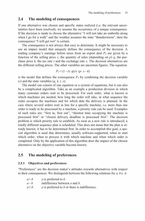
Figure 2-9 shows an example. A company needs to decide whether to continue or to abort the development of a new product. The probability of successfully completing the development is 0.3. If successful, the company needs to decide whether to develop large or small production capacities. The probability of high demand for the newly developed product is 0.6 while the probability of a low de-mand is 0.4.

Small capacity

Large capacity

0.6

0.4

High demand 1

Low demand 2

0.6

0.4

High demand 3

Low Demand 4

0.3

0.7

Success

Failure 5

Stopdevelopment

Continue development

6

Decision about product development

Figure 2-9: Decision tree for the product development problem

Due to a lack of space, the consequences are only labeled with numbers. For an exact description, the respective values of the objective variables have to be given. If the objective was purely financial, for instance, consequence 2 could follow from the development costs, investment costs for constructing the large production capacity and the marginal returns from the sales in the case of low demand.

Representing a decision situation in a decision tree usually provides some de-sign flexibility. On the one hand, complex alternatives can be split up into subse-quent actions. For example, a company whose space capacities do not suffice any-more could think about either expanding the building at hand, purchasing some ground and constructing a new building, or purchasing an already completed building. For each of these alternatives, two variants can be distinguished. They

- (a) of Figure 2-10. Obviously, how-ever, the alternative actions can equivalently be pre - r-natives, as can be seen in part (b) of the figure.


Use available extension plan

Replan

Just additional space

For total space

Build only for personal needs

Build for personal needs plus renting

Buy a building

Buy plot of landfor a new building

Extend existing building

(a)

Extend existing building using existing plans

Extend existing building using new plans

Buy a building just for additional space

Buy a new building for total space

Buy a plot of land and construct a building for personal needs

Buy a plot of land, construct for both personal needs and renting(b)

Figure 2-10: Equivalent representation of alternatives

On the other hand, events can be combined or split up. In a situation where a com-pany faces the risk of running out of raw material, because of an impending strike

a-bilities of a strike (and its length) first. In a second step, the conditional probabili-ties of material shortage are assessed for both a short and a long strike. Fig-ure 2-10 contains two equivalent representations (a) and (b) for this case. In part (b), the probabilities result from multiplying the probabilities for the different durations of a strike with the conditional probabilities for the possible material supply consequences in part (a).

If, for the problem at hand, the strike itself is irrelevant and only the material

mutually exclusive cases from part (b) and are represented in part (c) of Fig-ure 2-11.


0.3

0.5

Short strike0.2

Long strike

No strike

0.2

0.8

Shortage of material

No shortage

0.9

0.1


No shortage

(a)

(b)

No strike

Short strike, shortage

Short strike, no shortage

Long strike, shortage

Long strike, no shortage

0.49

0.51


No shortage(c)

Figure 2-11: Equivalent representation of events

All the strategies a decision maker has at hand can be read off the decision tree. To describe a strategy, the decision maker has to specify for each decision that could occur which alternative he would choose if he were to reach this point in the decision process. To depict a strategy in a decision tree, you would thus need to mark at each square, one (and only one) of the lines extending to the right. Return-ing to the example from Figure 2-

g-ure 2-12. Overall, this procedure would produce four different combinations of ar-rows (2 × 2). Obviously, however, we can condense two of these strategies, be-

decision in the second stage will be purely hypothetical, as it cannot be achieved in the tree anymore. In the example of product development, there are thus three strategies to consider:

a. Continue development. If successful, provide large capacity, b. Continue development. If successful, provide small capacity, c. Abort development.


Smallcapacity

Largecapacity

0.6

0.4

High demand 1

Low demand 2

0.6

0.4

High demand 3

Low demand 4

0.3

0.7

Success

Failure 5

Stopdevelopment

Continuedevelopment

6


Figure 2-12: Representation of a strategy in a decision tree

Likewise, the scenarios can be derived and depicted in the decision tree. Scenarios can be seen in a manner of speaking as our example, there are again four possible strategies with two of them condensa-ble.3 The following three scenarios remain:

1. Development successful, high demand, 2. Development successful, low demand, 3. Development unsuccessful.

Figure 2-13 depicts scenario 2.

3 Strictly speaking, the three uncertainty knots, each with two possible events, produce eight dif-ferent combinations (2 × 2 × 2). However, chance cannot select different paths for the two knots

probably a safe assumption). Therefore, the number of sensible combinations is reduced to four.


0.3Small capacity

Large capacity 0.4

High demand 1

Low demand 2

0.4

High demand 3

Low demand 4

Success

Failure 5

Stopdevelopment

Continuedevelopment

6


0.6

0.6

0.7

Figure 2-13: Representation of a scenario in a decision tree

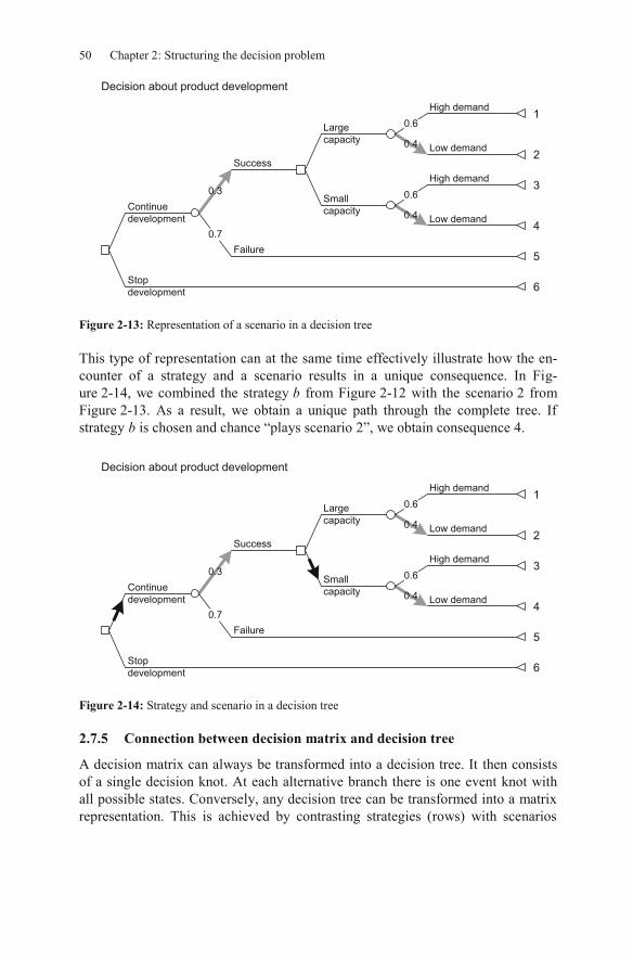
This type of representation can at the same time effectively illustrate how the en-counter of a strategy and a scenario results in a unique consequence. In Fig-ure 2-14, we combined the strategy b from Figure 2-12 with the scenario 2 from Figure 2-13. As a result, we obtain a unique path through the complete tree. If strategy b 4.

Small capacity

Large capacity 0.4

High demand 1

Low demand 2

0.4

High demand 3

Low demand 4

0.3

Success

Failure 5

Stop development

Continue development

6


0.7

0.6

0.6

Figure 2-14: Strategy and scenario in a decision tree

2.7.5 Connection between decision matrix and decision tree

A decision matrix can always be transformed into a decision tree. It then consists of a single decision knot. At each alternative branch there is one event knot with all possible states. Conversely, any decision tree can be transformed into a matrix representation. This is achieved by contrasting strategies (rows) with scenarios

Questions and exercises 51

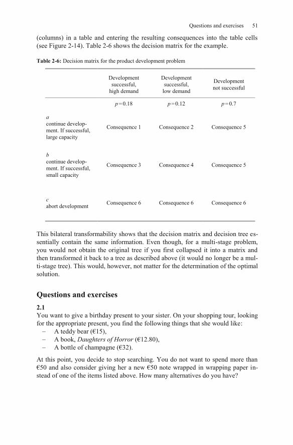
(columns) in a table and entering the resulting consequences into the table cells (see Figure 2-14). Table 2-6 shows the decision matrix for the example.

Table 2-6: Decision matrix for the product development problem

Development

successful, high demand

Development successful,

low demand

Development not successful

p = 0.18 p = 0.12 p = 0.7

a continue develop-ment. If successful, large capacity

Consequence 1 Consequence 2 Consequence 5

b continue develop-ment. If successful, small capacity

Consequence 3 Consequence 4 Consequence 5

c abort development Consequence 6 Consequence 6 Consequence 6

This bilateral transformability shows that the decision matrix and decision tree es-sentially contain the same information. Even though, for a multi-stage problem, you would not obtain the original tree if you first collapsed it into a matrix and then transformed it back to a tree as described above (it would no longer be a mul-ti-stage tree). This would, however, not matter for the determination of the optimal solution.

Questions and exercises 2.1 You want to give a birthday present to your sister. On your shopping tour, looking for the appropriate present, you find the following things that she would like:

A , A book, Daughters of Horror , A .

At this point, you decide to stop searching. You do not want to spend more than n-

stead of one of the items listed above. How many alternatives do you have?


2.2 You read a newspaper article about an unemployed citizen of Lazyville who has won the state lottery. You have hopes that the person mentioned in the article is your unsuccessful cousin Peter who lives in Lazyville. Thirty percent of the popu-lation of Lazyville are foreigners and the unemployment rate is 8%. Fifteen per-cent of the foreigners are unemployed. What is the probability of the winner being a native (i.e. not a foreigner)?

2.3 You think about wearing your new leather jacket on the way to the gym as you would like to show it to your friend who you might meet there. Unfortunately, a number of valuables have been stolen recently. There is a possibility that your jacket might be stolen while you are training.

(a) Which scenarios are relevant to this decision problem? (b) You estimate the probability of meeting your friend at the gym to be 60%

and the probability of your jacket being stolen to be 10%. What are the probabilities of the scenarios identified in (a)?

2.4 There are two events, x and y. Given the joint probabilities p(x,y) = 0.12; p(x,¬y) = 0.29 and the conditional probability p(y|¬x) = 0.90 (¬ indicates the com-plementary event).

(a) Calculate the probabilities p(¬x,¬y), p(¬x,y), p(x), p(y), p(¬x), p(¬y), p(x|y), p(y|x), and p(x|¬y).

(b) Calculate the probability p(x or y), i.e. the probability of at least one event occurring?

2.5 Your brother in law Calle Noni runs an Italian Restaurant. Recently, he has been complaining about his decreasing profits. As you are studying business adminis-tration, he asks you for advice. You do not know very much about his restaurant and plan to visit Calle to gather as much information as possible. For preparation, draw a cause tree containing all possible reasons for a decrease in profits.

2.6 On Friday morning, the owner of a restaurant thinks about how many cakes he should order for Sunday. In the event that the national team reaches the finals, he expects only a few guests and the sale of only two cakes. If the national team loses the semi-final on Friday afternoon, he expects to sell 20. The purchase price per

o maxim-ize his profit. Generate a decision matrix.

2.7 You want to go shopping and think about whether you should take an umbrella. If it rains and you do not have an umbrella, you will have to take your clothes to the

Questions and exercises 53

dry cleaner. On the other hand, you hate carrying an umbrella and often leave it behind at a shop. As the weather forecast will be on the radio soon, you think about postponing the decision.

(a) Structure the problem by drawing a decision tree. Indicate alternatives, events, and consequences.

(b) Is it also possible to depict the problem in the form of a decision matrix?

2.8 (a) How many strategies are in the following decision tree? (b) Pick one of them and mark its possible consequences. (c) How many scenarios are included in this decision tree? (d) Indicate one of the scenarios by marking all events which happen in this

scenario.

a3

a5

a4

a6

a7

d1

d2

a8

a10

a9

a11

a12

d3

d4

a1

a2


2.9 You think about donating a fraction of your million Euro inheritance to create a sports and leisure center. Clearly, the economic success of such a center depends on many factors. Depict them in an influence diagram.

55

Source: Bell (1984), pp. 17-23.

An American public utility holding company, the New England Electric System (NEES), was pondering whether to a ship that had ran aground off the coast of Florida in 1981. The ship could be used to haul coal from Virginia to its coal-powered stations in New England. However, a law that had passed in 1920 restricted American coastwise trade solely to vessels built, owned and operated by Americans; t , however, was a British ship. Another law from 1852 provided a way out: it permitted a foreign-built ship to be regarded as American-built if the previous owners declared the ship a total loss

three times the salvage value of the ship.

However, it was unknown on what basis the US Coast Guard, who was the re-sponsible authority, would determine the salvage value. The scrap value of the

i-dered the amount of the winning bid as an indication of the shivalue and NEES chose to bid more than $5 million, they would have to find some way to increase the cost of repairs accordingly. One way to increase the cost of re-pairs was to install self-unloading equipment in the ship. This would cost an extra $21 million and shorten the round trip voyage from 8 days to 5, which would be beneficial. However, the presence of the equipment would also lower the storage capacity, which would be unfavorable. It was uncertain how the Coast Guard would decide; NEES attached a probability of 70% to the bid price and 30% to the scrap value.

far, the profitability of the acquisition was highly dependent on the freight rates that could be charged for additional transports from external clients.

As for the chances to be awarded the contract, NEES was sure that a bid of $10 million would win and that a bid of $3 million definitely would not. For the values in between, the following probabilities were assumed:

$5m $6m $7m $8m $9m Probability 1/6 2/6 3/6 4/6 5/6

-unloading equipment, two offers from American shipbuilders regarding new ships were available.

The situation is depicted in the following decision tree. For simplification, only the offers of $5, $7, and $9 million were plotted and uncertainties regarding the freight rates were not depicted. The numbers marking the consequences stand for the expected net present values of the investment. Since one of the offers for building a new ship proved to be superior, the other one was not considered any-more.


1/6

5/6

Bid won 0.7

0.3

Salvage value = bid $6.6m

Salvage value = $5m $6.6m

$2.1mBid lost New ship

1/2

1/2

Bid won 0.7

0.3




5/6

1/6

Bid won0.3




Bid $5m

Bid $7m

Bid $9m

0.7

winning bid was $10 million. The Coast Guard valued the ship at its scrap value, but issued a ruling that future valuations could be expected to be significantly above scrap value.

Case Study 2: Development of global energy consumption 57

Case Study 2: A Scenario analysis about the development of global energy consumption and methods of power generation in the near future

Source: RAND (2001).

In the year 2000, the Office of Energy Efficiency and Renewable Energy (EERE) of the U.S. Department of Energy (DOE) hosted the so-called -congress in order to assemble a group of experts to discuss the world-wide chal-lenges relating to sufficient energy supply on a global scale. From this congress, the EERE expected an impulse for the implementation of an adequate and future-oriented energy policy.

Within the scope of this congress, the RAND Corporation was asked to conduct a scenario analysis on the basis of the most important drivers for the development of global energy consumption. For this purpose, RAND compiled a large number of existing energy scenarios and sorted them by specific parameters into different groups in order to identify a number of plausible scenarios for the future. These scenarios could then again be compared on the basis of the previously introduced parameters.

In concrete terms RAND proceeded as follows: in the beginning, three main categories of environmental factors were defined (sociopolitical, economic, and energy parameters) which were in turn further split up in order to allow the gener-ation of different meta-scenarios:

Sociopolitical Parameters

1. Potential for disruption (high, medium or low) 2. Energy contribution to the Consumer Price Index (percent) 3. Cost of health and environmental impacts and regulatory compliance

($/MBTU4)

Economic Parameters

1. Gross domestic product (GDP) growth (percent) 2. Inflation rate (percent per year) 3. Energy price inflation/overall price inflation (ratio) 4. Fuel taxes, energy subsidies, and R&D expenditures ($/MBTU)

Energy Parameters

1. Total energy consumption (quadrillion BTUs per year) 2. Decarbonization (dimensionless) 3. Energy productivity of the economy ($GDP/MBTU)

In general, it could be observed that the scenarios were very different, mostly due to the variety of the input parameters and the variability of the potential future de-velopments. However, four meta-scenarios (Business-as-Usual, Technological 4 MBTU is the abbreviation for Million British Thermal Units.


Improvement, High-Tech-Future and New Society) were created out of the afore-mentioned existing energy scenarios. For instance -as-

rowth and a higher environmental impact. This scenario extrapolated current trends in energy growth and productivity, whereby a decreasing use of nuclear power and hence an increase in the use of fossil fuels and a lower promotion of alternative energies were assumed. Additionally, another scenario (Hard Times) was created in order to integrate unexpected negative de-velopments into the analysis. This scenario was effectively not supposed to reflect actual beliefs about future developments but to serve as a kind of stress test.

Such a scenario analysis can be very helpful in a political decision-making process, for example to develop hedging strategies for potential threats of negative environmental impacts or to enable policymakers to better judge the consequences of their decisions (e.g. concerning the promotion of alternative energies).

rational decision making - readingsample

Documents