rational solutions of riccati-like partial differential equations
TRANSCRIPT

MM Research Preprints, 166–187No. 18, Dec. 1999. Beijing
Rational Solutions of Riccati-like Partial
Differential Equations1)
Ziming LiMMRC, Institute of Systems Science
Academia Sinica, Beijing 100080, ChinaEmail: [email protected]
Fritz SchwarzGMD, Institut SCAI
53754 Sankt Augustin, GermanyEmail: [email protected]
Abstract. When factoring linear partial differential systems with a finite-dimensionalsolution space or analyzing symmetries of nonlinear ode’s, we need to look for rationalsolutions of certain nonlinear pde’s. The nonlinear pde’s are called Riccati-like becausethey arise in a similar way as Riccati ode’s. In this paper we describe the structure ofrational solutions of a Riccati-like system, and an algorithm for computing them. Thealgorithm is also applicable to finding all rational solutions of Lie’s system ∂xu + u2 +a1u+a2v+a3, ∂yu+uv+b1u+b2v+b3, ∂xv+uv+c1u+c2v+c3, ∂yv+v2+d1u+d2v+d3,where a1 . . . d3 are rational functions of x and y.
1. Introduction
Riccati’s equation is one of the first examples of a differential equation that has beenconsidered extensively in the literature, shortly after Leibniz and Newton had introducedthe concept of the derivative of a function at the end of the 17th century. Riccati equationsoccur in many problems of mathematical physics and pure mathematics. A good survey isgiven in the book by Reid (1972).
Of particular importance is the relation between Riccati’s equation and a linear odey′′+ay′+by = 0 with a, b ∈ C(x), where C is the field of the complex numbers. For example,solutions h with the property that the quotient p = h′/h ∈ C(x) may be represented ash = exp (
∫p dx) if p satisfies the first-order Riccati equation p′+p2+ap+b = 0. Equivalently,
this linear ode allows the first-order right factor y′−qy over C(x) if q obeys the same equationas p. In general, finding the first-order right rational factors of a linear homogeneous ode isequivalent to finding the rational solutions of its associated Riccati equation (see e.g. Singer1991).
It turns out that this correspondence carries over to systems of linear homogeneous partialdifferential equations with a finite-dimensional solution space. Systems of this kind occur
1) The work is done when the first author visited GMD from September, 1997 to December, 2000
Rational Solutions of Riccati-like Systems 167
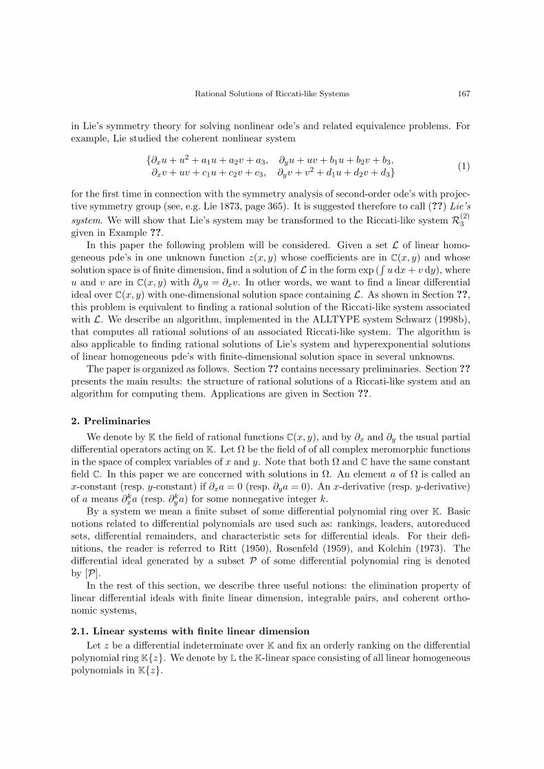
in Lie’s symmetry theory for solving nonlinear ode’s and related equivalence problems. Forexample, Lie studied the coherent nonlinear system
∂xu + u2 + a1u + a2v + a3, ∂yu + uv + b1u + b2v + b3,∂xv + uv + c1u + c2v + c3, ∂yv + v2 + d1u + d2v + d3
(1)
for the first time in connection with the symmetry analysis of second-order ode’s with projec-tive symmetry group (see, e.g. Lie 1873, page 365). It is suggested therefore to call (??) Lie’ssystem. We will show that Lie’s system may be transformed to the Riccati-like system R(2)
3
given in Example ??.In this paper the following problem will be considered. Given a set L of linear homo-
geneous pde’s in one unknown function z(x, y) whose coefficients are in C(x, y) and whosesolution space is of finite dimension, find a solution of L in the form exp (
∫u dx + v dy), where
u and v are in C(x, y) with ∂yu = ∂xv. In other words, we want to find a linear differentialideal over C(x, y) with one-dimensional solution space containing L. As shown in Section ??,this problem is equivalent to finding a rational solution of the Riccati-like system associatedwith L. We describe an algorithm, implemented in the ALLTYPE system Schwarz (1998b),that computes all rational solutions of an associated Riccati-like system. The algorithm isalso applicable to finding rational solutions of Lie’s system and hyperexponential solutionsof linear homogeneous pde’s with finite-dimensional solution space in several unknowns.
The paper is organized as follows. Section ?? contains necessary preliminaries. Section ??presents the main results: the structure of rational solutions of a Riccati-like system and analgorithm for computing them. Applications are given in Section ??.
2. Preliminaries
We denote by K the field of rational functions C(x, y), and by ∂x and ∂y the usual partialdifferential operators acting on K. Let Ω be the field of of all complex meromorphic functionsin the space of complex variables of x and y. Note that both Ω and C have the same constantfield C. In this paper we are concerned with solutions in Ω. An element a of Ω is called anx-constant (resp. y-constant) if ∂xa = 0 (resp. ∂ya = 0). An x-derivative (resp. y-derivative)of a means ∂k
xa (resp. ∂kya) for some nonnegative integer k.
By a system we mean a finite subset of some differential polynomial ring over K. Basicnotions related to differential polynomials are used such as: rankings, leaders, autoreducedsets, differential remainders, and characteristic sets for differential ideals. For their defi-nitions, the reader is referred to Ritt (1950), Rosenfeld (1959), and Kolchin (1973). Thedifferential ideal generated by a subset P of some differential polynomial ring is denotedby [P].
In the rest of this section, we describe three useful notions: the elimination property oflinear differential ideals with finite linear dimension, integrable pairs, and coherent ortho-nomic systems,
2.1. Linear systems with finite linear dimensionLet z be a differential indeterminate over K and fix an orderly ranking on the differential
polynomial ring Kz. We denote by L the K-linear space consisting of all linear homogeneouspolynomials in Kz.

168 Z. Li and F. Schwarz
Given a linear system L ⊂ L, the linear dimension of [L] in Kz is the codimension ofL∩ [L] in L (Kolchin 1973, page 151). The general solution of L depends on a finite numberof unspecified constants if and only if the linear dimension of [L] is finite (Kolchin 1973, page152). To check if the linear dimension of [L] is finite, we compute a coherent autoreducedset A (Rosenfeld, 1959) such that [L] = [A]. This computation can be done by variousmethods such as: Janet bases (Janet 1920, Schwarz 1998a) the characteristic set method(Wu 1989, Li and Wang 1999), and Grobner bases for differential operators (Kandri-Rodyand Weispfennig) . The linear dimension of [L] is finite if and only if an x-derivative and ay-derivative of z appear as leaders of some elements of A.
We denote by Lx (resp. Ly) the subset of L consisting of differential polynomials involvingonly x-derivatives (resp. y-derivatives) of z. The following elimination property is well-known.
Lemma 2.1 Let L be a finite subset of L. If [L] is of finite linear dimension, then there isan algorithm for computing two nonzero elements [L] ∩ Lx and [L] ∩ Ly, respectively.
Proof. Compute a coherent autoreduced set A in L such that [L] = [A]. Assume that A isnot 1, for, otherwise, [L] is trivial. A finite base B of the K-linear space V = L/(L ∩ [L])consists of all differential monomials ∂i
x∂jyz that cannot be reduced w.r.t. A. Using A, we
can express any element of V as a K-linear combination of elements of B. Hence, we canfind smallest integer n such that z, ∂xz, . . . , ∂n
xz are K-linearly dependent, that is, we canfind a0, a1, . . . , an−1 ∈ K such that
Lx = a0z + a1∂xz + · · ·+ an−1∂n−1x z + ∂n
xz ∈ [L].
Similarly, we can find a nonzero linear differential polynomial in [L] ∩ Ly. 2
2.2. Integrable pairsTo describe the structure of rational solutions in Section ??, we define a pair of rational
functions (f, g) ∈ K × K to be integrable if ∂yf = ∂xg. For an integrable pair (f, g), theexpression H = exp (
∫f dx + g dy) defines an element of Ω unique up to a nonzero multi-
plicative constant. We regard H as an element of Ω when the value of the multiplicativeconstant is irrelevant to our discussion. Note that ∂xH/H = f and ∂yH/H = g.
Two integrable pairs (f, g) and (p, q) are said to be equivalent if there exists a nonzero h inK such that f−p = ∂xh/h and g−q = ∂yh/h. Write (f, g) ∼ (p, q) when they are equivalent.Since (f, g) ∼ (p, q) if and only if the ratio of exp (
∫f dx + g dy) and exp (
∫p dx + q dy) is a
rational function, ∼ is an equivalence relation on the set of integrable pairs. It is easy to verifythat, for integrable pairs (f1, g1), (p1, q1), (f2, g2), (p2, q2) and integers m, n, (f1, g1) ∼ (p1, q1)and (f2, g2) ∼ (p2, q2) implies (mf1 + nf2, mg1 + ng2) ∼ (mp1 + np2, mq1 + nq2).
An element a in Ω is said to be a hyperexponential if ∂xa/a and ∂ya/a belong to K. If ais a hyperexponential, (∂xa/a, ∂ya/a) is an integrable pair. Conversely, for an integrablepair (f, g), we may construct a hyperexponential exp (
∫f dx + g dy) in Ω. For an integrable
pair (f, g), define E(f,g) to be the C-linear space h exp (∫
f dx + g dy) |h ∈ K . A directcalculations shows that E(f,g) consists of all hyperexponentials a such that (∂xa/a, ∂ya/a) ∼(f, g). The following lemma is used to group rational solutions of a Riccati-like system.
Lemma 2.2 If (f1, g1), (f2, g2), . . . , (fn, gn) are mutually inequivalent integrable pairs, thesum of C-linear spaces E(f1,g1), E(f2,g2), . . . , E(fn,gn) is direct.

Rational Solutions of Riccati-like Systems 169
Proof. We proceed by induction. For n = 2, if E(f1,g1) ∩E(f2,g2) contains a nonzero elementa, (∂xa/a, ∂ya/a) ∼ (fi, gi), for i = 1, 2. Hence, (f1, g1) ∼ (f2, g2), a contradiction. The sumof E(f1,g1) and E(f2,g2) is direct.
Assume that the result is proved for lower values of n. If the sum of E(f1,g1), E(f2,g2),. . . , E(fn,gn) is not direct, there are nonzero z1 ∈ E(f2,g2), z2 ∈ E(f2,g2), . . . , zn ∈ E(fn,gn)
which are C-linearly dependent. By a possible rearrangement of indexes, we have
zn = c1z1 + c2z2 + · · ·+ cn−1zn−1 (2)
for some c1, c2, . . . , cn−1 ∈ C. Since z1, z2, . . . , zn−1 are linearly independent over C bythe induction hypothesis, Theorem 1 in Kolchin (1973, page 86) implies that there existderivatives θ1, θ2, . . . , θn−1 such that W = det(θizj) is nonzero, where 1 ≤ i ≤ n − 1 and1 ≤ j ≤ n−1. Since the zi’s are hyperexponentials, there exists rij ∈ K such that θjzi = rjizi.Applying θ1, θ2, . . . , θn−1 to (??) then yields a linear system
r11 r12 · · · r1,n−1
r21 r22 · · · r2,n−1
· · · · · ·rn−1,1 rn−1,2 · · · rn−1,n−1
c1z1
c2z2...cn−1zn−1
=
r1nzn
r2nzn...rn,n−1zn
whose coefficient matrix (rji) is of full rank because W 6= 0. Solving this system, we getcizi = sizn, where si ∈ K. Since ck 6= 0 for some k with 1 ≤ k ≤ n− 1, zk/zn is rational, so(fk, gk) ∼ (fn, gn), a contradiction. 2
2.3. Coherent orthonomic systemsA system P in a differential polynomial ring D is orthonomic if it is an autoreduced
set and any element of P is linear w.r.t. its leader and monic, or, equivalently, both initialand separant of any element in P is one. A linear autoreduced set can be considered asan orthonomic system. System (??) is orthonomic w.r.t. any orderly ranking on u and v.Systems studied in this paper are always orthonomic with respect to certain orderly rankingon their differential indeterminates and derivatives.
Let P be an orthonomic system in D. We recall the notions of ∆-polynomials andcoherence in Rosenfeld (1959) for P. Note that these two notions are originally defined forautoreduced sets and the name “∆-polynomial” is due to Boulier et. al (1995). Let P1 and P2
belong to P with the respective leaders θ1z and θ2z, where z is a differential indeterminate,and θ1, θ2 are derivatives. Then there exist derivatives φ1 and φ2 with minimal ordersφ1θ1 = φ2θ2. The ∆-polynomial of P1 and P2, denoted by ∆(P1, P2), is φ1P1 − φ2P2. Notethat ∆(P1, P2) is well-defined provided the leaders of P1 and P2 are derivatives of the sameindeterminate. The system P is coherent if, for every such pair P1, P2 in P, ∆(P1, P2) canbe written as a D-linear combination of derivatives of elements of P, in which each derivativehas its leader lower than φ1θ1z (in a preselected ranking).
To study orthonomic systems, we need to make sure that they cannot be formally reducedto non-orthonomic or trivial ones. Corollary 3 in Chapter I of Rosenfeld (1959) asserts thatan orthonomic system P is a characteristic set of [P] if and only if P is coherent. Hence,P cannot be formally reduced any further if it is reduced. By the same corollary, one caneasily show
170 Z. Li and F. Schwarz
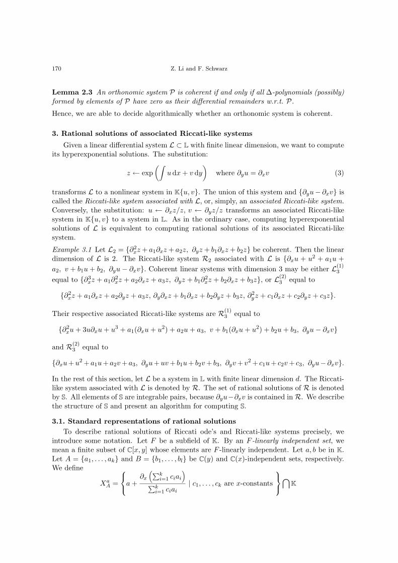
Lemma 2.3 An orthonomic system P is coherent if and only if all ∆-polynomials (possibly)formed by elements of P have zero as their differential remainders w.r.t. P.
Hence, we are able to decide algorithmically whether an orthonomic system is coherent.
3. Rational solutions of associated Riccati-like systems
Given a linear differential system L ⊂ L with finite linear dimension, we want to computeits hyperexponential solutions. The substitution:
z ← exp(∫
u dx + v dy
)where ∂yu = ∂xv (3)
transforms L to a nonlinear system in Ku, v. The union of this system and ∂yu− ∂xv iscalled the Riccati-like system associated with L, or, simply, an associated Riccati-like system.Conversely, the substitution: u ← ∂xz/z, v ← ∂yz/z transforms an associated Riccati-likesystem in Ku, v to a system in L. As in the ordinary case, computing hyperexponentialsolutions of L is equivalent to computing rational solutions of its associated Riccati-likesystem.
Example 3.1 Let L2 = ∂2xz + a1∂xz + a2z, ∂yz + b1∂xz + b2z be coherent. Then the linear
dimension of L is 2. The Riccati-like system R2 associated with L is ∂xu + u2 + a1u +a2, v + b1u + b2, ∂yu− ∂xv. Coherent linear systems with dimension 3 may be either L(1)
3
equal to ∂3xz + a1∂
2xz + a2∂xz + a3z, ∂yz + b1∂
2xz + b2∂xz + b3z, or L(2)
3 equal to
∂2xz + a1∂xz + a2∂yz + a3z, ∂y∂xz + b1∂xz + b2∂yz + b3z, ∂2
yz + c1∂xz + c2∂yz + c3z.
Their respective associated Riccati-like systems are R(1)3 equal to
∂2xu + 3u∂xu + u3 + a1(∂xu + u2) + a2u + a3, v + b1(∂xu + u2) + b2u + b3, ∂yu− ∂xv
and R(2)3 equal to
∂xu+u2 + a1u+ a2v + a3, ∂yu+uv + b1u+ b2v + b3, ∂yv + v2 + c1u+ c2v + c3, ∂yu−∂xv.
In the rest of this section, let L be a system in L with finite linear dimension d. The Riccati-like system associated with L is denoted by R. The set of rational solutions of R is denotedby S. All elements of S are integrable pairs, because ∂yu−∂xv is contained in R. We describethe structure of S and present an algorithm for computing S.
3.1. Standard representations of rational solutionsTo describe rational solutions of Riccati ode’s and Riccati-like systems precisely, we
introduce some notation. Let F be a subfield of K. By an F -linearly independent set, wemean a finite subset of C[x, y] whose elements are F -linearly independent. Let a, b be in K.Let A = a1, . . . , ak and B = b1, . . . , bl be C(y) and C(x)-independent sets, respectively.We define
XaA =
a +∂x
(∑ki=1 ciai
)∑k
i=1 ciai
| c1, . . . , ck are x-constants
⋂K

Rational Solutions of Riccati-like Systems 171
and
Y bB =
b +∂y
(∑li=1 cibi
)∑l
i=1 cibi
| c1, . . . , cl are y-constants
⋂K.
If, moreover, (a, b) is integrable and H = h1, . . . , hm is a C-linearly independent set, wedefine
S(a,b)H =
(a +
∂x (∑m
i=1 cihi)∑mi=1 cihi
, b +∂y (
∑mi=1 cihi)∑m
i=1 cihi
)| c1, . . . , cm ∈ C
.
Lemma 3.1 Let r1, r2, . . . , rk belong to C(y)[x] and c1, c2, . . . , ck be x-constants of Ω. If
f =c1∂xr1 + c2∂xr2 + · · ·+ ck∂xrk
c1r1 + c2r2 + · · ·+ ckrk
belongs to K, then there exist s1, s2, . . . , sk ∈ C[x, y] and d1, d2, . . . , dk ∈ C[y] such that
f =d1∂xs1 + d2∂xs2 + · · ·+ dk∂xsk
d1s1 + d2s2 + · · ·+ dksk.
Proof. Assume that f = f1/f2, where f1, f2 ∈ C[x, y]. Equating the coefficients of the likepowers of x in
(c1∂xr1 + c2∂xr2 + · · ·+ ck∂xrk)f2 = (c1r1 + c2r2 + · · ·+ ckrk)f1,
we find that c1, c2, . . . , ck satisfy a linear system over C(y). Hence, c1, c2, . . . , ck can be chosenas elements in C(y). Let h be the common denominator of all the ci and the ri. Then h isin C[y]. We derive that
f =h(c1∂xr1 + c2∂xr2 + · · ·+ ck∂xrk)
h(c1r1 + c2r2 + · · ·+ ckrk)=
d1∂xs1 + d2∂xs2 + · · ·+ dk∂xsk
d1s1 + d2s2 + · · ·+ dksk
where d1, d2, . . . , dk ∈ C[y] and s1, s2, . . . , sk ∈ C[x, y]. 2
By Lemma ?? the ci’s in XaA and Y b
B can be chosen as elements in C[y] and C[x], respec-tively. The next theorem describes the structure of S.
Theorem 3.2 There exist mutually inequivalent integrable pairs (a1, b1), . . . , (am, bm), andC-linearly independent sets H1, . . . ,Hm such that S is the (disjoint) union of S
(ai,bi)Hi
, i = 1,. . . , m. Moreover,
∑mi=1 |Hi| is no greater than d.
Proof. Let V be the solution space of L and (f1, g1), . . . , (fm, gm) in S, none of which isequivalent to the other. Then E(f1,g1) ∩ V , . . . , E(fm,gm) ∩ V are all nontrivial, and form adirect sum Lemma ??. Thus, m is no greater than d. We may further assume that there areonly m equivalence classes (w.r.t. ∼) in S.
Let (f, g) be one of the (fi, gi)’s. Assume that the intersection of V and E(f,g) is ofdimension k over C. Then there exist C-linearly independent rational functions r1, . . . , rk
such that r1 exp (∫
f dx + g dy) , . . . , rk exp (∫
f dx + g dy) form a basis for E(f,g) ∩ V . LetS(f,g) be the subset of S consisting of integrable pairs equivalent to (f, g). Then
S(f,g) =(
f +c1∂xr1 + · · ·+ ck∂xrk
c1r1 + · · ·+ ckrk, g +
c1∂yr1 + · · ·+ ck∂yrk
c1r1 + · · ·+ ckrk
)| c1, . . . , ck ∈ C
.
172 Z. Li and F. Schwarz
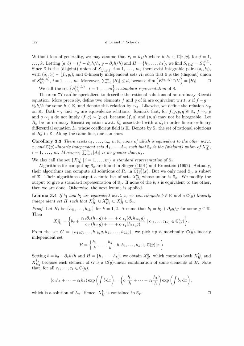
Without loss of generality, we may assume that rj = hj/h where h, hj ∈ C[x, y], for j = 1,. . . , k. Letting (a, b) = (f − ∂xh/h, g − ∂yh/h) and H = h1, . . . , hk, we find S(f,g) = S
(a,b)H .
Since S is the (disjoint) union of S(fi,gi), i = 1, . . . , m, there exist integrable pairs (ai, bi),with (ai, bi) ∼ (fi, gi), and C-linearly independent sets Hi such that S is the (disjoint) unionof S
(ai,bi)Hi
, i = 1, . . . , m. Moreover,∑m
i=1 |Hi| ≤ d, because dim(E(ai,bi) ∩ V
)= |Hi|. 2
We call the setS
(ai,bi)Hi
| i = 1, . . . ,m
a standard representation of S.Theorem ?? can be specialized to describe the rational solutions of an ordinary Riccati
equation. More precisely, define two elements f and g of K are equivalent w.r.t. x if f − g =∂xh/h for some h ∈ K, and denote this relation by ∼x. Likewise, we define the relation ∼y
on K. Both ∼x and ∼y are equivalence relations. Remark that, for f, g, p, q ∈ K, f ∼x pand g ∼y q do not imply (f, g) ∼ (p, q), because (f, g) and (p, q) may not be integrable. LetRx be an ordinary Riccati equation w.r.t. ∂x associated with a dxth order linear ordinarydifferential equation Lx whose coefficient field is K. Denote by Sx the set of rational solutionsof Rx in K. Along the same line, one can show
Corollary 3.3 There exists a1, . . . , am in K, none of which is equivalent to the other w.r.t.x, and C(y)-linearly independent sets A1, . . . , Am such that Sx is the (disjoint) union of Xai
Ai,
i = 1, . . . , m. Moreover,∑m
i=1 |Ai| is no greater than dx.
We also call the set XaiAi| i = 1, . . . ,m a standard representation of Sx.
Algorithms for computing Sx are found in Singer (1991) and Bronstein (1992). Actually,their algorithms can compute all solutions of Rx in C(y)(x). But we only need Sx, a subsetof K. Their algorithms output a finite list of sets Xbi
Hiwhose union is Sx. We modify the
output to give a standard representation of Sx. If none of the bi’s is equivalent to the other,then we are done. Otherwise, the next lemma is applied.
Lemma 3.4 If b1 and b2 are equivalent w.r.t. x, we can compute b ∈ K and a C(y)-linearlyindependent set H such that Xb1
H1∪Xb2
H2⊂ Xb
H ⊂ Sx.
Proof. Let Hi be hi1, . . . , hiki for k = 1, 2. Assume that b1 = b2 + ∂xg/g for some g ∈ K.
ThenXb1
H1=
b2 +c11∂x(h11g) + · · ·+ c1k1(∂xh1k1g)
c11(h11g) + · · ·+ c1k1(h1k1g)| c11, . . . c1k1 ∈ C(y)
.
From the set G = h11g, . . . , h1k1g, h21, . . . , h2k2, we pick up a maximally C(y)-linearlyindependent set
B =
h1
h, . . . ,
hk
h| h, h1, . . . , hk,∈ C(y)[x]
Setting b = b2 − ∂xh/h and H = h1, . . . , hk, we obtain Xb
H , which contains both Xb1H1
andXb2
H2because each element of G is a C(y)-linear combination of some elements of B. Note
that, for all c1, . . . , ck ∈ C(y),
(c1h1 + · · ·+ ckhk) exp(∫
b dx
)=(
c1h1
h+ · · ·+ ck
hk
h
)exp
(∫b2 dx
),
which is a solution of Lx. Hence, XbH is contained in Sx. 2
Rational Solutions of Riccati-like Systems 173
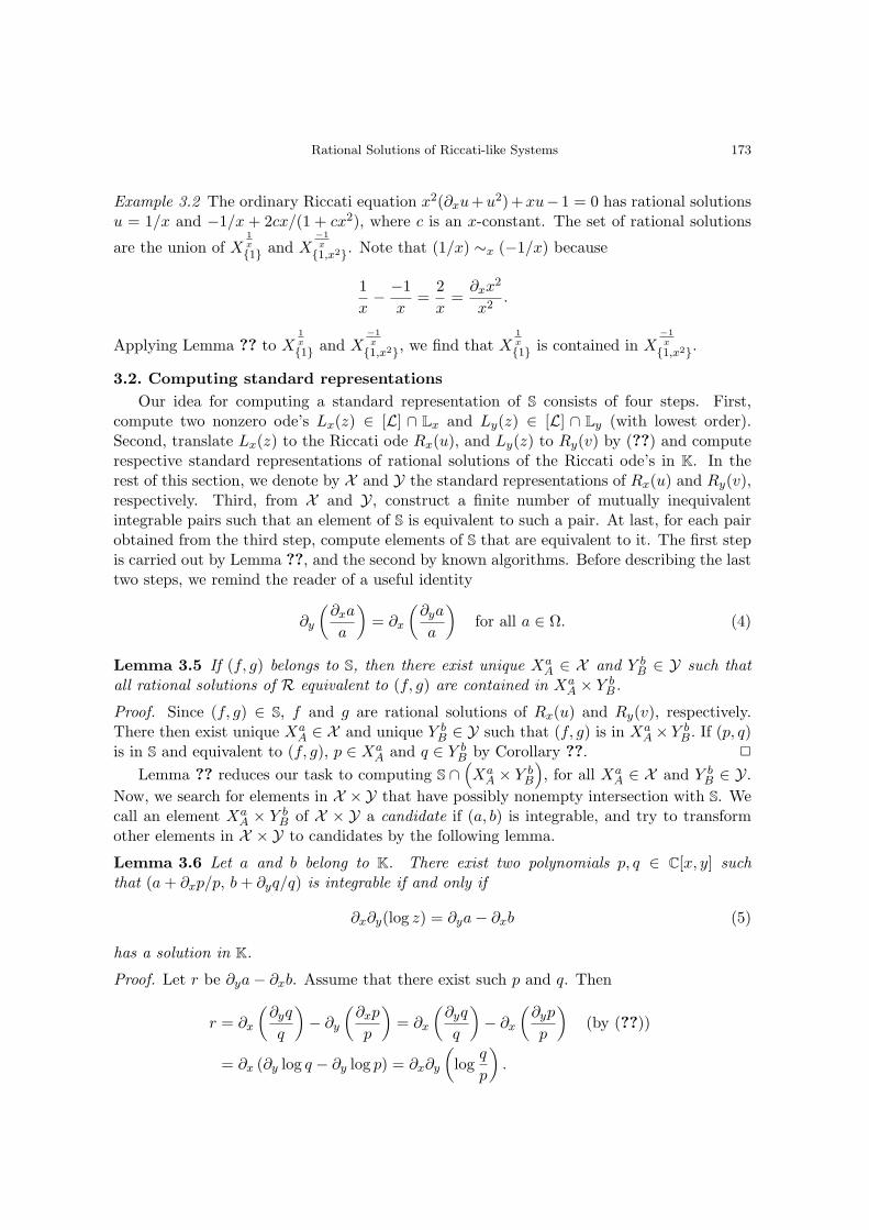
Example 3.2 The ordinary Riccati equation x2(∂xu+u2)+xu− 1 = 0 has rational solutionsu = 1/x and −1/x + 2cx/(1 + cx2), where c is an x-constant. The set of rational solutions
are the union of X1x
1 and X−1x
1,x2. Note that (1/x) ∼x (−1/x) because
1x− −1
x=
2x
=∂xx2
x2.
Applying Lemma ?? to X1x
1 and X−1x
1,x2, we find that X1x
1 is contained in X−1x
1,x2.
3.2. Computing standard representationsOur idea for computing a standard representation of S consists of four steps. First,
compute two nonzero ode’s Lx(z) ∈ [L] ∩ Lx and Ly(z) ∈ [L] ∩ Ly (with lowest order).Second, translate Lx(z) to the Riccati ode Rx(u), and Ly(z) to Ry(v) by (??) and computerespective standard representations of rational solutions of the Riccati ode’s in K. In therest of this section, we denote by X and Y the standard representations of Rx(u) and Ry(v),respectively. Third, from X and Y, construct a finite number of mutually inequivalentintegrable pairs such that an element of S is equivalent to such a pair. At last, for each pairobtained from the third step, compute elements of S that are equivalent to it. The first stepis carried out by Lemma ??, and the second by known algorithms. Before describing the lasttwo steps, we remind the reader of a useful identity
∂y
(∂xa
a
)= ∂x
(∂ya
a
)for all a ∈ Ω. (4)
Lemma 3.5 If (f, g) belongs to S, then there exist unique XaA ∈ X and Y b
B ∈ Y such thatall rational solutions of R equivalent to (f, g) are contained in Xa
A × Y bB.
Proof. Since (f, g) ∈ S, f and g are rational solutions of Rx(u) and Ry(v), respectively.There then exist unique Xa
A ∈ X and unique Y bB ∈ Y such that (f, g) is in Xa
A× Y bB. If (p, q)
is in S and equivalent to (f, g), p ∈ XaA and q ∈ Y b
B by Corollary ??. 2
Lemma ?? reduces our task to computing S ∩(Xa
A × Y bB
), for all Xa
A ∈ X and Y bB ∈ Y.
Now, we search for elements in X ×Y that have possibly nonempty intersection with S. Wecall an element Xa
A × Y bB of X × Y a candidate if (a, b) is integrable, and try to transform
other elements in X × Y to candidates by the following lemma.
Lemma 3.6 Let a and b belong to K. There exist two polynomials p, q ∈ C[x, y] suchthat (a + ∂xp/p, b + ∂yq/q) is integrable if and only if
∂x∂y(log z) = ∂ya− ∂xb (5)
has a solution in K.
Proof. Let r be ∂ya− ∂xb. Assume that there exist such p and q. Then
r = ∂x
(∂yq
q
)− ∂y
(∂xp
p
)= ∂x
(∂yq
q
)− ∂x
(∂yp
p
)(by (??))
= ∂x (∂y log q − ∂y log p) = ∂x∂y
(log
q
p
).

174 Z. Li and F. Schwarz
Conversely, if z = q/p is a solution of (??), reversing the above calculation shows that(a +
∂xp
p, b +
∂yq
q
)is integrable. 2
Now, we present an algorithm for computing such p and q.
Algorithm IntegrablePair (Find an integrable pair). Given a, b in K, the algorithm findsp, q in C[x, y] such that (a + ∂xp/p, b + ∂yq/q) is integrable, or determines that no such pand q exist.
I1. [Initialize.] Set r ← ∂ya− ∂xb. If r = 0, set p← 1, q ← 1 and exit.
I2. [Hermite’s reduction.] Apply Hermite’s reduction (w.r.t. x) to get f, h ∈ K such that
r = ∂xf + h (6)
If h is nonzero, the algorithm terminates; no such p and q exist.
I3. [Partial fraction.] Compute the irreducible partial fraction decomposition of f w.r.t. yover its coefficient field. If the decomposition is∑
i
mi∂yqi
qi−∑j
nj∂ypj
pj+ g (7)
where pi, qj ∈ C[x, y], mi, nj ∈ Z+ ∪ 0, and g ∈ C(y), set p ←∏
j pnj
j , q ←∏
i qmii .
Otherwise, no such p and q exist. 2
Step I1 is clear. If h 6= 0, then∫
r dx is not rational by Hermite’s reduction (Geddes, et.al 1992, Bronstein 1997). Thus, (??) has no rational solution, and such p and q do not existby Lemma ??. Suppose now h = 0. Equations (??) and (??) imply that
∂yz
z= f + w (8)
where w is an x-constant. Assume that the irreducible partial fraction decomposition of fw.r.t. y is
f =∑j
nj∂yqj
qj−∑
i
mi∂ypi
pi︸ ︷︷ ︸G
+∑k
sk
tk+ r︸ ︷︷ ︸
g
, (9)
where pi, qi, sk, tk, r ∈ C[x, y], pi, qi, tk are irreducible over C(x)[y] and relatively prime to eachother. If z is rational, then the partial decomposition of ∂yz/z is of form G, so that g mustbe an x-constant because of (??), (??) and the uniqueness of partial fraction decomposition.Suppose now that g belongs to C(y). We compute
∂y
(a +
∂xp
p
)− ∂x
(b +
∂yq
q
)= r + ∂y
(∂xp
p
)− ∂x
(∂yq
q
)(??)= r + ∂x
(∂yp
p− ∂yq
q
)(??)= ∂x
(f +
∂yp
p− ∂yq
q
)(??)= ∂xg = 0.
IntegrablePair then returns p and q, as desired.

Rational Solutions of Riccati-like Systems 175
Example 3.3 Given
a =y2x3 + x3 + xy2 + y − x2y − x
yx3 + y2x4 − x5y − x4and b =
1x− y
,
IntegrablePair proceeds as follows.
I1. r = 1/(1 + xy)2.
I2. f = −1/(xy2 + y), h = 0.
I3. f = x/(1 + xy)− 1/y, p = 1, q = 1 + xy.
Hence,(a, b + x
1+xy
)is integrable.
Example 3.4 Apply IntegrablePair to
a =y3 + xy2 + 2y − x2y − x
xy3 + y2 − x2y2 − xyand b =
1x− y
.
We find that
r = − x2y2 + 2xy + 1− y2
x2y4 + 2xy3 + x2y4 + y2and f = −x2y + x + y
y2(xy + 1).
In step I3 f decomposes intox
1 + xy− 1
y− x
y2.
Since g = −x/y2 is not in C(y), no such p and q exist.
In what follows, by “given XaA×Y b
B”, we mean that we are given a, b ∈ K, a C(y)-linearlyindependent set A, and a C(x)-linearly independent set B.
The set XaA × Y b
B contains no rational solutions of R if IntegrablePair confirms thatno p, q ∈ C[x, y] are such that (a+∂xp/p, b+∂yq/q) is integrable, because a rational solutionof R must be integrable. Otherwise, we construct a candidate described below.
Algorithm Candidate (Find a solution candidate). Given XaA × Y b
B, the algorithm findsXf
F × Y gG such that (f, g) is an integrable pair and Xf
F × Y gG = Xa
A × Y bB, or determines that
XaA × Y b
B contains no integrable pairs.
C1. [construct f and g.] If IntegrablePair(a, b) returns p, q ∈ C[x, y], set
f ← a− ∂xq
q, g ← b− ∂yp
p.
Otherwise, the algorithm terminates; XaA × Y b
B contains no integrable pairs.
C2. [construct F and G.] Set F ← qh | h ∈ A, G← ph | h ∈ B. 2

176 Z. Li and F. Schwarz
In Step C1 we set the integrable pair (f, g) to be (a− ∂xq/q, b− ∂yp/p) instead of (a +∂xp/p, b + ∂yq/q), because the former construction makes step C2 simpler. Equation (??)implies that (f, g) is integrable if (a + ∂xp/p, b + ∂yq/q) is. To see Xf
F × Y gG = Xa
A × Y bB, we
let α =∑
s∈A css, where the cs’s are in C[y], not all zero. Since a + ∂xα/α = f + ∂x(qα)/qα,
XfF = Xa
A. Likewise, Y gG = Y b
B. The algorithm Candidate is correct.
Example 3.5 Let a and b be the same as those in Example ??. Let A = 1, x and B = 1.IntegrablePair(a, b) returns p = 1 and q = 1+xy. Candidate then returns f = a−y/(1+xy), g = b, F = 1 + xy, x(1 + xy) and G = B.
Applying the above algorithm to each member of X × Y, we obtain a set of disjointcandidates
C =Xf1
F1× Y g1
G1, . . . , Xfk
Fk× Y gk
Gk
such that S is contained in
(Xf1
F1× Y g1
G1
)⋃· · ·⋃(
XfkFk× Y gk
Gk
), and a rational solution of R
can belong to only one member in C.Lemma 3.7 Let Xf
F × Y gG be one of the sets in C. Let
ex = maxp∈F
degx p and ey = maxq∈G
degy q.
If an integrable pair (a, b) belongs to XfF ×Y g
G, then there exists a polynomial h ∈ C[x, y] withdegx h ≤ ex and degy h ≤ ey such that
(a, b) =(
f +∂xh
h, g +
∂yh
h
). (10)
Proof. Let (a, b) = (f + ∂xs/s, g + ∂yt/t) , where s and t are, respectively, C(y)- and C(x)-linear combinations of elements in F and G. Since (a, b) and (f, g) are integrable pairs, sois (∂xs/s, ∂yt/t) . The function
h = exp(∫
∂xs
sdx +
∂yt
tdy
)is well-defined and has the property ∂xh/h = ∂xs/s and ∂yh/h = ∂yt/t. It follows that
s = ah and t = bh (11)
for some x-constant a and y-constant b. Consequently, sb = ta. Let α be an element of Csuch that t(α, y) 6= 0. Then a = s(α, y)b(α)/t(α, y), which implies that a belongs to C(y),and, therefore, h is in C(y)[x] by (??). Likewise, h is in C(x)[y]. Hence, h is in C[x, y].Accordingly, degx h = degx s ≤ ex and degy h = degy t ≤ ey by (??). 2
Suppose that (a, b) is a rational solution of R contained in XfF ×Y g
G. By Lemma ?? thereexists h ∈ C[x, y] such that (??) holds. Moreover, respective degree bounds for h in x and yare known. The next algorithm PolynomialPart determines h.
Algorithm PolynomialPart (Find polynomial part). Given an associated Riccati-likesystem R, and a candidate Xf
F × Y gG, the algorithm computes a C-linearly independent set
H such that the set of rational solutions of R equivalent to (f, g) is equal to S(f,g)H . If H is
empty, then such rational solutions do not exist.

Rational Solutions of Riccati-like Systems 177
P1. [bound degrees.] Set ex ← maxp∈F degx p, ey ← maxq∈G degy q.
P2. [ex = ey = 0.] If both ex and ey are zero, check whether (f, g) satisfies all the equationsin R; if the answer is affirmative, set H ← 1, otherwise, set H ← ∅; the algorithmterminates.
P3. [form a linear algebraic system.] Set h ←∑ex
i=0
∑ey
j=0 cijxiyj , where the cij are un-
specified constants. Substitute a + ∂xh/h and b + ∂yh/h for u and v in each equationof R, respectively. Set L be the result, which is a linear homogeneous algebraic systemin the cij ’s.
P4. [compute H.] Calculate a basis B for the solution space of L. If B consists of onlyzero vector, then set H ← ∅. Otherwise, set H to be the set consisting of polynomialscorresponding to vectors of B. 2
In Step P3 substituting u← a+∂xh/h, v ← b+∂yh/h into R is equivalent to substitutingz ← h exp (f dx + g dy) into L; the latter yields a linear homogeneous system in the unspec-ified constants cij ’s, because exp (f dx + g dy) is a nonzero overall factor. Thus, L obtainedin step P3 is a linear homogeneous algebraic system. The correctness of PolynomialPartthen follows from Lemma ??.
Example 3.6 Determine the rational solutions of
R =
∂xu + u2 − 2
xu +
2y2 − 2y
x2v +
2x2
, ∂yu + uv, ∂yv + v2 +2
y − 1v, ∂yu− ∂xv
.
in S1 = X01, x x2 × Y
−1y−1
y−1, 1 and S2 = Xy1, x × Y x
1, y, respectively. Applying Polynomial-Part to S1 yields
P1. ex = 2 and ey = 1.
P2. Skipped.
P3. h = c0 + c1x + c2y + c3x2 + c4xy + c5x
2y, u ← ∂xh/h, v ← −1/(2y) + ∂yh/h, L =c0, c4 + c1, c5 + c3.
P4. H = y, x− xy, x2 − x2y.
The rational solutions in X01, x x2 × Y
−1y−1
y−1, 1 are(c2(1− y) + 2c3x(1− y)
c1y + c2(x− xy) + c3(x2 − x2y), − 1
y − 1+
c1 − c2x− c3x2
c1y + c2(x− xy) + c3(x2 − x2y)
)
where c1, c2, c3 ∈ C.
Applying PolynomialPart to S2 yields
P1. ex = 1 and ey = 1.
P2. Skipped.
178 Z. Li and F. Schwarz
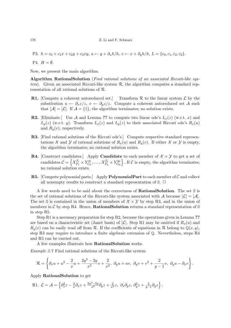
P3. h = c0 + c1x + c2y + c3xy, u← y + ∂xh/h, v ← x + ∂yh/h, L = c0, c1, c2, c3.
P4. H = ∅.
Now, we present the main algorithm.
Algorithm RationalSolution (Find rational solutions of an associated Riccati-like sys-tem). Given an associated Riccati-like system R, the algorithm computes a standard rep-resentation of all rational solutions of R.
R1. [Compute a coherent autoreduced set.] Transform R to the linear system L by thesubstitution u ← ∂xz/z, v ← ∂yz/z. Compute a coherent autoreduced set A suchthat [A] = [L]. If A = 1, the algorithm terminates; no solution exists.
R2. [Eliminate.] Use A and Lemma ?? to compute two linear ode’s Lx(z) (w.r.t. x) andLy(z) (w.r.t. y). Transform Lx(z) and Ly(z) to their associated Riccati ode’s Rx(u)and Ry(v), respectively.
R3. [Find rational solutions of the Riccati ode’s.] Compute respective standard represen-tations X and Y of rational solutions of Rx(u) and Ry(v). If either X or Y is empty,the algorithm terminates; no rational solution exists.
R4. [Construct candidates.] Apply Candidate to each member of X × Y to get a set ofcandidates C =
Xf1
F1× Y g1
G1, . . . , Xfk
Fk× Y gk
Gk
. If C is empty, the algorithm terminates;
no rational solution exists.
R5. [Compute polynomial parts.] Apply PolynomialPart to each member of C and collectall nonempty results to construct a standard representation of S. 2
A few words need to be said about the correctness of RationalSolution. The set S isthe set of rational solutions of the Riccati-like system associated with A because [L] = [A].The set S is contained in the union of members of X × Y by step R3, and in the union ofmembers in C by step R4. Hence, RationalSolution returns a standard representation of Sin step R5.
Step R1 is a necessary preparation for step R2, because the operations given in Lemma ??are based on a characteristic set (Janet basis) of [L]. Step R1 may be omitted if Rx(u) andRy(v) can be easily read off from R. If the coefficients of equations in R belong to Q(x, y),step R3 may require to introduce a finite algebraic extension of Q. Nevertheless, steps R4and R5 can be carried out.
A few examples illustrate how RationalSolution works.
Example 3.7 Find rational solutions of the Riccati-like system
R =
∂xu + u2 − 2
xu +
2y2 − 2y
x2v +
2x2
, ∂yu + uv, ∂yv + v2 +2
y − 1v, ∂yu− ∂xv
.
Apply RationalSolution to get
R1. L = A =∂2
xz − 2x∂xz + 2y2−2y
x2 ∂yz + 2x2 z, ∂x∂yz, ∂2
yz + 2y−1∂yz
.
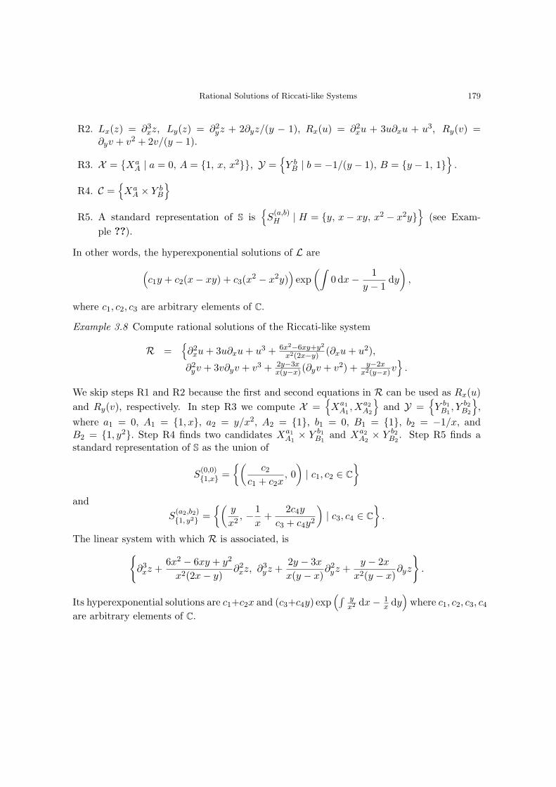
Rational Solutions of Riccati-like Systems 179
R2. Lx(z) = ∂3xz, Ly(z) = ∂2
yz + 2∂yz/(y − 1), Rx(u) = ∂2xu + 3u∂xu + u3, Ry(v) =
∂yv + v2 + 2v/(y − 1).
R3. X =Xa
A | a = 0, A = 1, x, x2, Y =
Y b
B | b = −1/(y − 1), B = y − 1, 1
.
R4. C =Xa
A × Y bB
R5. A standard representation of S is
S
(a,b)H | H = y, x− xy, x2 − x2y
(see Exam-
ple ??).
In other words, the hyperexponential solutions of L are(c1y + c2(x− xy) + c3(x2 − x2y)
)exp
(∫0 dx− 1
y − 1dy
),
where c1, c2, c3 are arbitrary elements of C.
Example 3.8 Compute rational solutions of the Riccati-like system
R =∂2
xu + 3u∂xu + u3 + 6x2−6xy+y2
x2(2x−y)(∂xu + u2),
∂2yv + 3v∂yv + v3 + 2y−3x
x(y−x)(∂yv + v2) + y−2xx2(y−x)
v
.
We skip steps R1 and R2 because the first and second equations in R can be used as Rx(u)and Ry(v), respectively. In step R3 we compute X =
Xa1
A1, Xa2
A2
and Y =
Y b1
B1, Y b2
B2
,
where a1 = 0, A1 = 1, x, a2 = y/x2, A2 = 1, b1 = 0, B1 = 1, b2 = −1/x, andB2 = 1, y2. Step R4 finds two candidates Xa1
A1× Y b1
B1and Xa2
A2× Y b2
B2. Step R5 finds a
standard representation of S as the union of
S(0,0)1,x =
(c2
c1 + c2x, 0)| c1, c2 ∈ C
and
S(a2,b2)1, y2 =
(y
x2, −1
x+
2c4y
c3 + c4y2
)| c3, c4 ∈ C
.
The linear system with which R is associated, is∂3
xz +6x2 − 6xy + y2
x2(2x− y)∂2
xz, ∂3yz +
2y − 3x
x(y − x)∂2
yz +y − 2x
x2(y − x)∂yz
.
Its hyperexponential solutions are c1+c2x and (c3+c4y) exp(∫ y
x2 dx− 1x dy
)where c1, c2, c3, c4
are arbitrary elements of C.

180 Z. Li and F. Schwarz
4. Applications
In this section we apply the algorithm RationalSolution to finding rational solutions ofLie’s system and hyperexponential solutions of linear homogeneous differential systems withfinite linear dimension in several unknowns.
Lie’s system (??) occurred originally in his investigation of certain second-order ode’sthat were based on its symmetries (Lie 1873). It turned out to be almost as ubiquitous asthe Riccati ode’s, e.g. in decomposing systems of linear pde’s into smaller components.
To extend the applicability of the algorithm, we consider the following more generalorthonomic system
P1 = ∂xu + a0u2 + a1u + a2v + a3, P2 = ∂yu + b0uv + b1u + b2v + b3,
P3 = ∂xv + c0uv + c1u + c2v + c3, P4 = ∂yv + d0v2 + d1u + d2v + d3
(12)
in Ku, v w.r.t. the ranking 1 < v < u < ∂yv < ∂xv < ∂yu < ∂xu < · · ·. Moreover, weassume that both a0 and d0 are nonzero.
The differential remainders of ∆(P1, P2) and ∆(P3, P4) are, respectively,
R12 = b0(c0 − a0)vu2 + a2(b0 − d0)v2 + terms involving u2, uv, u, v, 1
andR34 = c0(d0 − b0)v2u + d1(a0 − c0)u2 + terms involving v2, uv, u, v, 1.
Observe that R12 and R34 are in K[u, v]. Hence, if either R12 or R34 is nonzero, all solu-tions of (??) would be solutions of some polynomials in K[u, v]. We will not consider thisdegenerating case.
Lemma 4.1 If (??) is coherent, either a0 = c0 and b0 = d0, or b0 = c0 = a2 = d1 = 0.
Proof. If (??) is coherent, R12 = R34 = 0 by Lemma ??. Hence
b0(c0 − a0) = a2(b0 − d0) = c0(d0 − b0) = d1(a0 − c0) = 0.
Since a0d0 6= 0 in (??), either a0 = c0 and b0 = d0, or b0 = c0 = a2 = d1 = 0. 2 Lemma ??splits (??) into two systems
F1 = ∂xu + a0u2 + a1u + a2v + a3, F2 = ∂yu + d0uv + b1u + b2v + b3,
F3 = ∂xv + a0uv + c1u + c2v + c3, F4 = ∂yv + d0v2 + d1u + d2v + d3
(13)
andG1 = ∂xu + a0u
2 + a1u + a3, G2 = ∂yu + b1u + b2v + b3,G3 = ∂xv + c1u + c2v + c3, G4 = ∂yv + d0v
2 + d2v + d3.(14)
Note that Lie’s system is a special case of (??). Clearly, the coherence of (??) implies thecoherence of (??) and (??). We solve (??) and (??) separately.
Theorem 4.2 If (??) is coherent, then the substitution
u← 1a0
U − 13a0
(a1 + c2 −
∂x(a0d0)a0d0
), v ← 1
d0V − 1
3d0
(b1 + d2 −
∂y(a0d0)a0d0
)(15)
transforms (??) into an associated Riccati-like system (in U and V ) of type R(2)3 in Exam-
ple ??

Rational Solutions of Riccati-like Systems 181
Proof. Normalizing (??) by the substitution
u← u
a0, v ← v
d0, (16)
we transform (??) into the coherent system
F1 = ∂xu + u2 + a1u + a2v + a3, F2 = ∂yu + uv + b1u + b2v + b3,F3 = ∂xv + uv + c1u + c2v + c3, F4 = ∂yv + v2 + d1u + d2v + d3,
(17)
where a1, . . . , d3 ∈ K. Since the differential remainders of ∆(F1, F2) and ∆(F3, F4) are,respectively,
R12 = (c1 − b1)u2 + (c2 − b2)uv + (c3 + b2c1 + ∂ya1 − ∂xb1 − 2b3 − a2d1)︸ ︷︷ ︸p
u
+ terms involving v and 1,
and
R34 = (c1 − b1)uv + (c2 − b2)v2 + (2c3 − b2c1 − b3 + a2d1 − ∂xd2 + ∂y c2)︸ ︷︷ ︸q
v
+ terms involving u and 1,
we deduce b1 = c1, b2 = c2 and p = q = 0. It follows that
p + q = 3c3 + ∂y(a1 + c2)− 3b3 − ∂x(b1 + d2) = 0. (18)
Applying the substitution
u← U − s, v ← V − t, where s = 13(a1 + c2) and t = 1
3(b1 + d2) (19)
to (??), we get
f1 = ∂xU + U2 + A1U + A2V + A3, f2 = ∂yU + UV + B1U + B2V + B3,f3 = ∂xV + UV + C1U + C2V + C3, f4 = ∂yV + V 2 + D1U + D2V + D3
(20)
where A1, . . . , D3 ∈ K. Since b1 = c1 and b2 = c2, B1 = C1 and B2 = C2. We compute
B3 − C3 = (−∂ys− b1s− b2t + st + b3)− (−∂xt− c1s− c2t + st + c3)= b3 + ∂xt− c3 − ∂ys (since b1 = c1 and b2 = c2)
=13(3b3 + ∂x(b1 + d2)− 3c3 − ∂y(a1 + c2)
)(by (??))
= 0 (by (??)).
Therefore, f2 − f3 = ∂yU − ∂xV . This implies that f1, f2, f2 − f3, f4 is the associatedRiccati-like system R(2)
3 , so is (??). Since
a1 = a1 − ∂xa0/a0, c2 = c2 − ∂xd0/d0, b1 = b1 − ∂ya0/a0, d2 = d2 − ∂xd0/d0,
substitution (??) is the result of the composition of (??) and (??). 2

182 Z. Li and F. Schwarz
Example 4.1 Consider the coherent Lie’s system
∂xu + u2 +y + x2
x(y − x2)u +
4y(y + x2)x2(y − x2)
v +6yx2 + x4 + 4y2
x2(y2 − 2yx2 + x4)= 0,
∂yu + uv +1
y − x2u− 2y + x2
x(y − x2)v − 2(y + x2)
x(y2 − 2yx2 + x4)= 0,
∂xv + uv +1
y − x2u− 2y + x2
x(y − x2)v +
x2 − 2y
x(y2 − 2yx2 + x4)= 0,
∂yv + v2 +4
y − x2v +
2y2 − 2yx2 + x4
= 0.
By (??) we apply the transformation
u← U +y
3x(y − x2), v ← V − 5
3(y − x2)
to get
∂xU + U2 +5y + 3x2
3x(y − x2)U +
4y(y + x2)x2(y − x2)
V +9x4 + 6yx2 − 23y2
9x2(y2 − 2yx2 + x4)= 0,
∂yU + UV − 23(y − x2)
U − 5y + 3x2
3x(y − x2)V +
2(5y − 3x2)9x(y2 − 2yx2 + x4)
= 0,
∂xV + UV − 23(y − x2)
U − 5y + 3x2
3x(y − x2)V +
2(5y − 3x2)9x(y2 − 2yx2 + x4)
= 0,
∂yV + V 2 +2
3(y − x2)V − 2
9(y2 − 2yx2 + x4)= 0,
which is equivalent to the Riccati-like system R(2)3 in Example ??, because the difference
between the second and third equations is ∂yU − ∂xV . Apply RationalSolution to thissystem to find the rational solutions:
U =−13x
+2x
3(y − x2)+
2c2x
c1y + c2x2, V =
−13(y − x2)
+c1
c1y + c2x2, c1, c2 ∈ C.
Hence, the rational solutions of the original system are
u =x
y − x2+
2c2x
c1y + c2x2, v =
−2y − x2
+c1
c1y + c2x2, c1, c2 ∈ C.
We turn our attention to (??).
Theorem 4.3 If (??) is coherent, it decouples into two individual coherent systems
∂xu + a0u2 + a1u + a3, ∂yu + b1u + b3 ∂yv + d0v
2 + d2v + d3, ∂xv + c2v + c3 (21)
for u and v, respectively.

Rational Solutions of Riccati-like Systems 183
Proof. The differential remainders of ∆(G1, G2) and ∆(G3, G4) are, respectively
R12 = −2b2a0uv + terms involving u2, u. v and 1
andR34 = 2c1d0uv + terms involving v2, u. v and 1
Since (??) is coherent, b2 = c1 = 0. The theorem follows. 2
The following system also appears frequently in symmetry analysis.
Theorem 4.4 Let a1, . . . , b3 ∈ K and a1b1 6= 0. The first-order Riccati-like system
F = ∂xz + a1z2 + a2z + a3, G = ∂yz + b1z
2 + b2z + b3 (22)
is coherent if and only if its general solution depends on a single constant. If (??) has arational solution, one of the following alternatives applies.
1. The general solution is rational and has the form
1a1
∂xr
r + c+ p =
1b1
∂yr
r + c+ p
with p, r ∈ K and c ∈ C ∪ ∞.
2. There are at most two special rational solutions not involving unspecified constants.
Proof. Since the differential remainder of ∆(F,G) is an algebraic polynomial in K[z] of degreeno greater than 2, (??) has at most two solutions if it is not coherent.
Assume that (??) is coherent. We show that it is the system R2 in disguise (see Exam-ple ??). The substitution
z ← 1a1
u− 12a1
(a2 −
∂xa1
a1
)(23)
transforms (??) into the coherent system
f = ∂xu + u2 + A3, g = ∂yu + B1u2 + B2u + B3, (24)
where A3, B1, B2, B3 ∈ K. Since the differential remainder of ∆(f, g) is zero,
B2 = −∂xB1, ∂xB2 = 2A3B1 − 2B3,
which implies
g −B1f = ∂yu−B1∂xu− (∂xB1)u +12∂2
xB1 = ∂yu− ∂x
(B1u−
12∂xB1
).
Hence, (??) is equivalent to the system∂xu + u2 + A3, ∂yu− ∂x
(B1u−
12∂xB1
).

184 Z. Li and F. Schwarz
Set v =(B1w − 1
2∂xB1
). The above system becomes
∂xu + u2 + A3, v −B1u +12∂xB1, ∂yu− ∂xv
(25)
which is of type R2 in Example (??). It follows from (??) and the definition of v that (u, v)is a solution of (??) if and only if z given in (??) is a solution of (??). Since (??) is associatedwith a coherent linear system with linear dimension two, the general solution of (??) can bewritten as
(u, v) =(
c1∂xs1 + c2∂xs2
c1s1 + c2s2,
c1∂ys1 + c2∂ys2
c1s1 + c2s2
),
where s1 and s2 are in some differential extension F of K, linearly independent over theconstant field of F, and c1 and c2 are in the same constant field. Therefore, (??) implies thatthe general solution of (??) can be written as
z =1a1
c1∂xs1 + c2∂xs2
c1s1 + c2s2− 1
2a1
(a2 −
∂xa1
a1
).
Setting c = c1/c2, we prove that the general solution of (??) depends on one constant.We now consider the rational solutions of (??). By (??) and the second equation in (??),
z is a rational solution of (??) if and only if (u, v) is a rational solution of (??). By Theo-rem ?? (??) has either infinitely many rational solutions or at most two inequivalent rationalsolutions The former case corresponds to the first alternative, and the latter to the second.Assume that (??) has infinitely many rational solutions. Then, by Theorem ??,
(u, v) =(
c1∂xh1 + c2∂xh2
c1h1 + c2h2+ a,
c1∂yh1 + c2∂yh2
c1h1 + c2h2+ b
)where h1, h2, a, b ∈ K and c1, c2 ∈ C. Setting r = h2/h1, c = c1/c2, f = ∂xh1/h1 + a andg = ∂yh1/h1 + b, we get
(u, v) =(
∂xr
c + r+ f,
∂yr
c + r+ g
).
Transformation (??) implies that
z =1a1
∂xr
c + r+ p
for some p ∈ K. Substituting ∂yr/(c + r) + g for v in the second equation of (??) yields
z =1
a1B1
∂yr
c + r+ q
for some q ∈ K. Hence, p = q because we may set c = ∞, i.e., c2 = 0. The theorem is thenproved by noticing that a1B1 = b1. 2 According to the proof of Theorem ??,the rational solutions of (??) can be computed by the algorithm RationalSolution. Wemay also proceed as follows. Compute the rational solutions of F . If there are only a finitenumber of solutions, we need only check if they satisfy G. Otherwise, the rational solutionsof F are given by
∂xr
C + r+ f

Rational Solutions of Riccati-like Systems 185
where r, f ∈ K and C ∈ C(y). Substituting this expression for z in G yields
H = ∂yC + B1C2 + B2C + B3,
for some B1, B2, B3 ∈ K. Collecting coefficients of H w.r.t. the powers of x yields a system inC(y)C consisting possibly of first-order Riccati ode’s, first-order linear ode’s and algebraicequations, whose rational solutions can be easily found.
Example 4.2 Compute the rational solutions of
∂xz + z2, ∂yz + (1− x2 − 2xy − y2)z2 + (2x + 2y)z − 1 = 0.
The rational solutions of the first equation are 1/(C(y) + x), where C(y) is an x-constant.Substituting the expression into the second equation yields
∂yC(y) + C(y)2 − 2yC(y) + y2 − 1 = 0,
so that C(y) = y + 1/(y + c), where c is a constant. This system has the rational solutions
z =1
x + y + 1y+c
=∂x
(xy+y2+1
x+y
)c + xy+y2+1
x+y
+1
x + y.
At last, the following problem is considered. Let D be the differential polynomial ringKz1, . . . , zn. Given a linear system L ⊂ D with finite linear dimension, find all hyperexpo-nential solutions of L. By general elimination procedures, we compute a linear characteristicset Li for [L] ∩ Kzi, for i = 1, . . . , n. Since each [Li] is also of finite linear dimension, thealgorithm RationalSolution computes a standard representation Si of the rational solutionsof the Riccati-like system associated with Li. Assume that
Si =S
(fij ,gij)Hij
| j = 1, . . . ,mi
.
The hyperexponential solutions of Li are then expressed as Ei =⋃mi
j=1 Vij , where
Vij =
∑
h∈Hij
chh
exp(∫
fij dx + gij dy
)| ch ∈ C
.
The problem is thus reduced to computing hyperexponential solutions of L contained in V1j1×· · · × Vnjn for 1 ≤ j1 ≤ m1, . . . , 1 ≤ jn ≤ mn. Substituting ∑
h∈Hiji
chh
exp(∫
fiji dx + giji dy
)
for zi in L yields a linear algebraic system A in the unspecified constants c’s. Notice that thecoefficients of A may be hyperexponential. Nevertheless, the constant solutions of A givesus the hyperexponential solutions of L in V1j1 × · · · × Vnjn .

186 Z. Li and F. Schwarz
Example 4.3 Consider the system L
x2∂xz2 − xy∂xz1 + yz1, x2∂2xz1 − x∂xz1 + z1,
y∂yz1 − x∂xz1 + z1, xy∂yz2 + xy∂xz1 − xz2 + yz1.
By elimination we get
L1 = y∂yz1 − x∂xz1 + z1, x2∂2xz1 − x∂xz1 + z1
andL2 = y∂yz2 − xy2∂xz2 − z2, x2∂3
xz2 + 3x∂2xz2 + ∂xz2.
By the algorithm RationalSolution we find that respective hyperexponential solutionsof L1 and L2 are c1x and c2y, where c1, c2 ∈ C. Substituting c1x for z1 and c2y for z2 intoL yields the linear system c1 = 0. Hence, the hyperexponential solutions of L are (0, c2y),where c2 ∈ C.
References
Boulier, F., Lazard, D., Ollivier, F., Petitot, M. (1995). Representation for the radical ofa finitely generated differential ideal. In: Levelt, A.H.M. (ed.): Proc. Int. Symp. onSymbolic and Algebraic Computation, Montreal, Canada, ACM Press, 158–166.
Bronstein, M. (1992). Linear ordinary differential equations: breaking through the order 2barrier. In: Wang. P. (ed.): Proc. Int. Symp. on Symbolic and Algebraic Computation,Berkeley, ACM Press, 42–48.
Bronstein, M. (1997). Symbolic Integration I: Transcendental Functions. Springer.Geddes, K., Czapor, S., Labahn, G. (1992). Algorithms for Computer Algebra. Kluwer
Academic Publishers.Janet, M. (1920). Les systems d’equations aux derivees partielles. Journal de mathematiques
83, 65–123.Kandru-Rody, A. Weispfenning, V. (1990). Non-commutative Grobner Bases in algebras of
solvable type. J. Symb. Comput. 9, 1–26.Kolchin, E. (1973). Differential Algebra and Algebraic Groups. New York: Academic Press.Li, Z., Wang, D.-m. (1999) Coherent, regular and simple systems in zero decompositions of
partial differential systems. Syst. Sci. Math. Sci. 12 Suppl., 43–60.Lie, S. Klassifikation und Integration von gewohnlichen Differentialgleichungen zwischen x,
y, die eine Gruppe von Transformationen gestatten III. Archiv for Mathematik VIII,371–458 (Gesammelte Abhandlungen V, 362–427).
Reid, W. T. (1972). Riccati Differential Equations. Academic Press, New York and London.Ritt, J. F. (1950). Differential Algebra. New York: Amer. Math. Soc.Rosenfeld, A. (1959). Specializations in differential algebra. Trans. Amer. Math. Soc. 90,
394–407.Schwarz, F. (1998a). Janet bases for symmetry groups. In: Buchberger, B. and Winkler, F.
(eds.): Grobner Bases and Applications, London Math. Soc. Lecture Notes Series 251.Cambridge: Cambridge University Press, 221–234.
Schwarz, F. (1998b). ALLTYPES: An ALgebraic Language and Type System. In: CalmetJ. and Plaza J. (eds.): Artificial Intelligence and Symbolic Computation, Lecture Notesin Artificial Intelligence 1476. Springer, 270 – 283.

Rational Solutions of Riccati-like Systems 187
Singer, M. (1991). Liouillian solutions of linear differential equations with Liouillian coeffi-cients. J. Symb. Comput. 11, 251–273.
Wu, W.-t. (1989). On the foundation of algebraic differential geometry. Syst. Sci. Math.Sci. 2, 289–312.