rc-1532 - development of specifications for the superpave simple

FINAL REPORT

Development of Specification for the Superpave Simple Performance Tests (SPT)

PI: Zhanping You, Ph.D., P.E. DEPARTMENT OF CIVIL AND ENVIRONMENTAL ENGINEERING

MICHIGAN TECHNOLOGICAL UNIVERSITY 1400 TOWNSEND DRIVE

HOUGHTON, MICHIGAN 49931

SUBMITTED TO

John W Barak, P.E. MICHIGAN DEPARTMENT OF TRANSPORTATION

CONSTRUCTION PAVING UNIT - C&T SECONDARY GOVERNMENTAL COMPLEX

8885 RICKS ROAD LANSING, MI 48909

May 2009

Technical Report Documentation Page 1. Project No. RC-1532

2. Government Accession No.

3. Recipient's Catalog No.

4. Title and Subtitle Development of Specifications for the Superpave Simple Performance Tests

5. Report Date May 16th, 2009

6. Performing Organization Code

7. Author(s) Zhanping You, Shu Wei Goh, and R. Christopher Williams

8. Performing Organization Report No.

9. Performing Organization Name and Address Michigan Technological University 1400 Townsend Drive Houghton, MI 49931

10. Work Unit No. (TRAIS) 11. Contract or Grant No. 06-0414/2

12. Sponsoring Agency Name and Address Michigan Department of Transportation Murray Van Wagoner Building 425 West Ottawa, P.O. Box 30050 Lansing, MI 48909

13. Type of Report and Period Covered Final Report 2006/7/13 - 2009/5/16 14. Sponsoring Agency Code

15. Supplementary Notes 16. Abstract This report describes the development and establishment of a proposed Simple Performance Test (SPT) specification in order to contribute to the asphalt materials technology in the state of Michigan. The properties and characteristic of materials, performance testing of specimens, and field analyses are used in developing draft SPT specifications. These advanced and more effective specifications should significantly improve the qualities of designed and constructed hot mix asphalt (HMA) leading to improvement in pavement life in Michigan. The objectives of this study include the following: 1) using the SPT, conduct a laboratory study to measure the parameters including the dynamic modulus terms (E*/sinϕ and E*) and the flow number (Fn) for typical Michigan HMA mixtures, 2) correlate the results of the laboratory study to field performance as they relate to flexible pavement performance (rutting, fatigue, and low temperature cracking), and 3) make recommendations for the SPT criteria at specific traffic levels (e.g. E3, E10, E30), including recommendations for a draft test specification for use in Michigan. The specification criteria of dynamic modulus were developed based upon field rutting performance and contractor warranty criteria. 17. Key Word

Hot mix paving mixtures, Superpave, Specifications, Flexible pavements, Performance evaluations

18. Distribution Statement No restrictions. This document is available to the public through the Michigan Department of Transportation

19. Security Classif. (of this report) Unclassified

20. Security Classif. (of this page) Unclassified

21. No. of Pages 220

22. Price n/a

Form DOT F 1700.7 (8-72) Reproduction of completed page authorized

ACKNOWLEDGEMENT

The research work was partially sponsored by Federal Highway Administration through

Michigan Department of Transportation. The researchers appreciate the guidance and

involvement of John Barak of the Michigan Department of Transportation as the Project

Manager. The researchers also acknowledge the support from Curtis Bleech, Timothy R.

Crook, John F. Staton, Michael Eacker, Steve Palmer, David R. Schade, Daniel J.

Sokolnicki, Larry Whiteside, and Pat Schafer of the Michigan Department of

Transportation, and John Becsey of the Asphalt Pavement Association of Michigan. The

researchers appreciate the donations of materials from many contractors.

The experimental work was completed in the Center of Excellence for Transportation

Materials at Michigan Technological University, which maintains the AASHTO

Materials Reference Laboratory (AMRL) accreditation on asphalt and asphalt mixtures,

aggregates, and Portland cement concrete. This center is funded jointly by the Michigan

Department of Transportation and Michigan Technological University.

The research work cannot be complete without the significant contribution of Dr. Thomas

Van Dam, former faculty at Michigan Technological University, Dr. Jianping Dong,

Edwin W. Tulppo Jr., James R. Vivian III, Julian Mills-Beale, and Baron Colbert in the

Center of Excellence for Transportation Materials. The researchers appreciate the

assistance of all the personal who contributed to this research project.

I

DISCLAIMER

This document is disseminated under the sponsorship of the Michigan Department

of Transportation (MDOT) in the interest of information exchange. MDOT assumes no

liability for its content or use thereof.

The contents of this report reflect the views of the contracting organization, which

is responsible for the accuracy of the information presented herein. The contents may not

necessarily reflect the views of MDOT and do not constitute standards, specifications, or

regulations.

II

TABLE OF CONTENT

DISCLAIMER ..................................................................................................................... I

LIST OF TABLES ............................................................................................................ IV

LIST OF FIGURES .......................................................................................................... VI

EXECUTIVE SUMMARY ................................................................................................ 1

CHAPTER 1: INTRODUCTION ....................................................................................... 4

Background ..................................................................................................................... 4

Problem Statements ........................................................................................................ 7

Objectives ....................................................................................................................... 9

CHAPTER 2: LITERATURE REVIEW .......................................................................... 10

Introduction ................................................................................................................... 10

Dynamic Modulus Literature Reviews ..................................................................... 15

Potential Uses of Dynamic Modulus in Pavement Rutting Performance ................. 17

Flow Number Literature Review .................................................................................. 18

CHAPTER 3: EXPERIMENTAL DESIGN ..................................................................... 21

Sample Collection ......................................................................................................... 23

Compaction Process ...................................................................................................... 25

Rice Test (Theoretical Maximum Specific Gravity) ................................................ 25

Bulk Specific Gravity and Air Void ......................................................................... 25

Estimating Gyration Number and Mixture Volumetric Property ............................. 25

Sample Fabrication ....................................................................................................... 30

III

Dynamic Modulus Test ................................................................................................. 32

Flow Number Test ........................................................................................................ 36

Loading Level used in Flow Number Test ............................................................... 37

Effective Rutting Temperature ................................................................................. 38

CHAPTER 4: TEST RESULTS AND FIELD INFORMATION .................................... 40

Introduction ................................................................................................................... 40

Dynamic Modulus Test Results .................................................................................... 41

Flow Number Test Results............................................................................................ 52

Field Rutting Results..................................................................................................... 53

Pavement Structure ....................................................................................................... 54

Traffic Information ....................................................................................................... 55

CHAPTER 5: ANALYSIS AND DISCUSSIONS ........................................................... 58

Introduction ................................................................................................................... 58

Analysis and Discussions of Dynamic Modulus Test Results ...................................... 59

Analysis of Flow Number Results ................................................................................ 64

Relationship between Deformation Rate and Stepwise Flow Number ..................... 69

Evaluation of Field Rutting Performance ..................................................................... 71

Evaluation of Traffic Data ............................................................................................ 75

Development of Trial Dynamic Modulus Specification ............................................... 77

Development of Trial Flow Number Specification .................................................... 105

CHAPTER 6: SUMMARY AND RECOMMENDATIONS ......................................... 108

REFERENCES ............................................................................................................... 112

IV

APPENDIX 1: PROJECT’S JOB MIX FORMULA ...................................................... 121

APPENDIX 2: MIXTURE’S VOLUMETRIC PROPERTIES ...................................... 136

APPENDIX 3: DYNAMIC MODULUS TEST RESULTS ........................................... 151

APPENDIX 4: DYNAMIC MODULUS MASTER CURVES ...................................... 181

APPENDIX 5: MINIMUM DYNAMIC MODULUS CRITERIA ................................ 211

LIST OF TABLES

Table 1 Experimental test method factorial for selecting the Simple Performance Test [18]

......................................................................................................................................... 7

Table 2 Simple Performance Test’s Advantages and Disadvantages ............................... 14

Table 3 Asphalt Mixture Information ............................................................................... 24

Table 4 Test Temperatures and Temperature Equilibrium Time for |E*| Test ................. 33

Table 5 Descriptors for each Asphalt Mixture .................................................................. 41

Table 6 Average Flow Number Measured using Stepwise Approach .............................. 52

Table 7 Field Rutting Results ........................................................................................... 53

Table 8 Pavement Structure and Maintenance or Construction Method of the Mixture

Collected from the Field ............................................................................................... 55

Table 9 Traffic Information for each Mixture .................................................................. 56

Table 10 Field Rutting Performance and Mixture’s Theoretical Pavement Rutting Life

Index ............................................................................................................................. 74

Table 11 Traffic Level for each Mixture Type ................................................................. 76

Table 12 Field Traffic Level and Design Life Index ........................................................ 76

V

Table 14 Mixtures That Meet the Warranty Specification ............................................... 78

Table 15 Mixtures That do not meets the Warranty Specification ................................... 78

Table 16 Dynamic Modulus for HMA Mixtures that meet Warranty Criteria and did not

meet Warranty Criteria at 39.2°C and 0.1Hz ................................................................ 82

Table 17 Ranking of Mixture with 4% Air Void Level based on Flow Number Slope at

45°C ............................................................................................................................ 105


45°C ............................................................................................................................ 106

Table 19 Flow Number Criteria for Mixture with 4% Air Void Level .......................... 107

Table 20 Flow Number Criteria for Mixture with 7% Air Void Level .......................... 107

Table 21 Minimum Dynamic Modulus Criteria for 4% Air Void Level Mixture at -5 ºC

..................................................................................................................................... 211

Table 22 Minimum Dynamic Modulus Criteria for 4% Air Void Level Mixture at 4 ºC

..................................................................................................................................... 212


..................................................................................................................................... 213

Table 24 Minimum Dynamic Modulus Criteria for 4% Air Void Level Mixture at 21.3 ºC

..................................................................................................................................... 214


..................................................................................................................................... 215


..................................................................................................................................... 216

VI


..................................................................................................................................... 217


..................................................................................................................................... 218


..................................................................................................................................... 219


..................................................................................................................................... 220

LIST OF FIGURES

Figure 1 Quality Control using Dynamic Modulus for Rutting Distress .......................... 18

Figure 2 General Flow Chart for the Experimental Design .............................................. 22

Figure 3 Sample Collection Areas in Michigan ................................................................ 23

Figure 4 Pine Gyratory Compactor ................................................................................... 26

Figure 5 Estimated and Corrected Bulk Specific Gravity for Trial Sample ..................... 27

Figure 6 Air Void Level for a Trial Sample ..................................................................... 29

Figure 7 Cutting and Coring Process ................................................................................ 30

Figure 8 Asphalt Mixture after Cutting and Coring process ............................................. 31

Figure 9 Dynamic Modulus Test Device (IPC UTM 100) ............................................... 32

Figure 10 Platen Loading Device ..................................................................................... 33

Figure 11 Dynamic Modulus Test Setup .......................................................................... 34

Figure 12 Sample Test Results of Dynamic Modulus Test .............................................. 35

Figure 13 Loading and unloading of Flow Number Test ................................................. 36

VII

Figure 14 Sample Fail after the Flow Number Test ......................................................... 37

Figure 15 MAAT Average and MAAT Standard Deviation in Michigan ........................ 39

Figure 16 Dynamic Modulus for 4% Air Void Level at -5°C .......................................... 42

Figure 17 Dynamic Modulus for 7% Air Void Level at -5°C .......................................... 43

Figure 18 Dynamic Modulus for 4% Air Void Level at 4°C ............................................ 44

Figure 19 Dynamic Modulus for 7% Air Void Level at 4°C ............................................ 45

Figure 20 Dynamic Modulus for 4% Air Void Level at 13°C ......................................... 46

Figure 21 Dynamic Modulus for 7% Air Void Level at 13°C .......................................... 47

Figure 22 Dynamic Modulus for 4% Air Void Level at 21.3°C ....................................... 48




Figure 26 Comparing |E*| with Various HMA Design Traffic Level at 21.3°C .............. 60

Figure 27 Comparing |E*| with Various HMA Design Traffic Level at 39.2°C .............. 60

Figure 28 Comparing |E*|/sinδ with Various HMA Design Traffic Level at 21.3°C ....... 61

Figure 29 Comparing |E*|/sinδ with Various HMA Design Traffic Level at 39.2°C ....... 61

Figure 30 Comparison of Dynamic modulus of different Nominal Maximum Aggregate

Size (NMAS) at 21.3°C and 0.1hz ................................................................................ 62

Figure 31 Comparison of Dynamic modulus of different Nominal Maximum Aggregate

Size (NMAS) at 39.2°C and 0.1hz ................................................................................ 63

Figure 32 Comparisons of Stepwise and Three-Stage Methods ....................................... 65

Figure 33 Comparison of Stepwise and Creep Stiffness times Cycles versus Cycles

Methods......................................................................................................................... 66

VIII

Figure 34 Comparison of Stepwise and FNest Methods .................................................. 67

Figure 35 Comparison of Stepwise and Traditional Methods .......................................... 68

Figure 36 Relationship of Flow Number and Rate of Deformation at Secondary Stage .. 70

Figure 37 Field Rutting Data (Maintenance occurred when rutting reached approximately

0.25 in.) ......................................................................................................................... 73

Figure 38 Specification of Dynamic Modulus at Various Traffic Levels and Aggregate

Sizes .............................................................................................................................. 83

Figure 39 Master Curve for Allowable |E*| for 3E10 HMA Mixture using the Referenced

Temperature of 21.3°C ................................................................................................. 84

Figure 40 Master Curve for Minimum Required Dynamic Modulus of 3E10 at 4% Air

Void Level .................................................................................................................... 85


Void Level .................................................................................................................... 86


Void Level .................................................................................................................... 87


Void Level .................................................................................................................... 88


Void Level .................................................................................................................... 89


Void Level .................................................................................................................... 90


Void Level .................................................................................................................... 91

IX


Void Level .................................................................................................................... 92


Void Level .................................................................................................................... 93


Void Level .................................................................................................................... 94


Void Level .................................................................................................................... 95


Void Level .................................................................................................................... 96


Void Level .................................................................................................................... 97


Void Level .................................................................................................................... 98


Void Level .................................................................................................................... 99


Void Level .................................................................................................................. 100


Void Level .................................................................................................................. 101


Void Level .................................................................................................................. 102

X


Void Level .................................................................................................................. 103


Void Level .................................................................................................................. 104

Figure 60 Dynamic Modulus for 3E10 I (Project Location: M-59 Brighton) at 4% Air

Void Level .................................................................................................................. 151

Figure 61 Dynamic Modulus for 3E10 I (Project Location: M-59 Brighton) at 7% Air

Void Level .................................................................................................................. 152

Figure 62 Dynamic Modulus for 3E10 II (Project Location: Michigan Ave, Dearborn) at

4% Air Void Level ...................................................................................................... 153


7% Air Void Level ...................................................................................................... 154

Figure 64 Dynamic Modulus for 3E30 I (Project Location: Vandyke, Detroit) at 4% Air

Void Level .................................................................................................................. 155


Void Level .................................................................................................................. 156

Figure 66 Dynamic Modulus for 4E1 I (Project Location: Tri Mt., Hancock) at 4% Air

Void Level .................................................................................................................. 157


Void Level .................................................................................................................. 158

Figure 68 Dynamic Modulus for 4E3 I (Project Location: Lansing, MI) at 4% Air Void

Level ........................................................................................................................... 159

XI


Level ........................................................................................................................... 160

Figure 70 Dynamic Modulus for 4E3 II (Project Location: Lexington) at 4% Air Void

Level ........................................................................................................................... 161


Level ........................................................................................................................... 162

Figure 72 Dynamic Modulus for 4E10 I (Project Location: M-53 Detroit) at 4% Air Void

Level ........................................................................................................................... 163


Level ........................................................................................................................... 164

Figure 74 Dynamic Modulus for 4E30 II (Project Location: 8 Mile Road) at 4% Air Void

Level ........................................................................................................................... 165


Level ........................................................................................................................... 166

Figure 76 Dynamic Modulus for 5E1 I (Project Location: M-26, Kearsarge St.) at 4% Air

Void Level .................................................................................................................. 167


Void Level .................................................................................................................. 168

Figure 78 Dynamic Modulus for 5E1 II (Project Location: M-38) at 4% Air Void Level

..................................................................................................................................... 169


..................................................................................................................................... 170

XII

Figure 80 Dynamic Modulus for 5E3 I (Project Location: Bessemer, MI) at 4% Air Void

Level ........................................................................................................................... 171


Level ........................................................................................................................... 172

Figure 82 Dynamic Modulus for 5E10 I (Project Location: Auburn Hills) at 4% Air Void

Level ........................................................................................................................... 173


Level ........................................................................................................................... 174

Figure 84 Dynamic Modulus for 5E10 II (Project Location: Oregon, OH) at 4% Air Void

Level ........................................................................................................................... 175


Level ........................................................................................................................... 176

Figure 86 Dynamic Modulus for 5E30 I (Project Location: I-75 Clarkston) at 4% Air

Void Level .................................................................................................................. 177

Figure 87 Dynamic Modulus for 5E30 I (Project Location: I-75 Clarkston) at 7% Air

Void Level .................................................................................................................. 178

Figure 88 Dynamic Modulus for 5E30 II (Project Location: I-75 Toledo) at 4% Air Void

Level ........................................................................................................................... 179


Level ........................................................................................................................... 180

Figure 90 Master Curve of Dynamic Modulus for 3E10 I (Project Location: M-59

Brighton) Mixture with 4% Air Void Level at the Reference Temperature of -5°C .. 181

XIII


Brighton) Mixture with 7% Air Void Level at the Reference Temperature of -5°C .. 182

Figure 92 Master Curve of Dynamic Modulus for 3E10 II (Project Location: Michigan

Ave, Dearborn) Mixture with 4% Air Void Level at the Reference Temperature of -

5°C .............................................................................................................................. 183

Figure 93 Master Curve of Dynamic Modulus for 3E10 II (Project Location: Michigan

Ave, Dearborn) Mixture with 7% Air Void Level at the Reference Temperature of -

5°C .............................................................................................................................. 184

Figure 94 Master Curve of Dynamic Modulus for 3E30 I (Project Location: Vandyke,

Detroit) Mixture with 4% Air Void Level at the Reference Temperature of -5°C ..... 185

Figure 95 Master Curve of Dynamic Modulus for 3E30 I (Project Location: Vandyke,


Figure 96 Master Curve of Dynamic Modulus for 4E1 I (Project Location: Tri Mt.,

Hancock) Mixture with 4% Air Void Level at the Reference Temperature of -5°C .. 187

Figure 97 Master Curve of Dynamic Modulus for 4E1 I (Project Location: Tri Mt.,

Hancock) Mixture with 7% Air Void Level at the Reference Temperature of -5°C .. 188

Figure 98 Master Curve of Dynamic Modulus for 4E3 I (Project Location: Lansing, MI)

Mixture with 4% Air Void Level at the Reference Temperature of -5°C .................. 189

Figure 99 Master Curve of Dynamic Modulus for 4E3 I (Project Location: Lansing, MI)


Figure 100 Master Curve of Dynamic Modulus for 4E3 II (Project Location: Lexington)


XIV

Figure 101 Master Curve of Dynamic Modulus for 4E3 II (Project Location: Lexington)






Figure 104 Master Curve of Dynamic Modulus for 4E30 II (Project Location: 8 Mile Rd)




Figure 106 Master Curve of Dynamic Modulus for 5E1 I (Project Location: M-26,

Kearsarge St.) Mixture with 4% Air Void Level at the Reference Temperature of -5°C

..................................................................................................................................... 197

Figure 107 Master Curve of Dynamic Modulus for 5E1 I (Project Location: M-26,

Kearsarge St.) Mixture with 7% Air Void Level at the Reference Temperature of -5°C

..................................................................................................................................... 198

Figure 108 Master Curve of Dynamic Modulus for 5E1 II (Project Location: M-38)


Figure 109 Master Curve of Dynamic Modulus for 5E1 II (Project Location: M-38)


Figure 110 Master Curve of Dynamic Modulus for 5E3 I (Project Location: Bessemer,

MI) Mixture with 4% Air Void Level at the Reference Temperature of -5°C ........... 201

XV

Figure 111 Master Curve of Dynamic Modulus for 5E3 I (Project Location: Bessemer,

MI) Mixture with 7% Air Void Level at the Reference Temperature of -5°C ........... 202

Figure 112 Master Curve of Dynamic Modulus for 5E10 I (Project Location: Auburn

Hills) Mixture with 4% Air Void Level at the Reference Temperature of -5°C ........ 203

Figure 113 Master Curve of Dynamic Modulus for 5E10 I (Project Location: Auburn

Hills) Mixture with 7% Air Void Level at the Reference Temperature of -5°C ........ 204

Figure 114 Master Curve of Dynamic Modulus for 5E10 II (Project Location: Oregon,

OH) Mixture with 4% Air Void Level at the Reference Temperature of -5°C .......... 205

Figure 115 Master Curve of Dynamic Modulus for 5E10 II (Project Location: Oregon,

OH) Mixture with 7% Air Void Level at the Reference Temperature of -5°C .......... 206

Figure 116 Master Curve of Dynamic Modulus for 5E30 I (Project Location: I-75

Clarkston) Mixture with 4% Air Void Level at the Reference Temperature of -5°C. 207

Figure 117 Master Curve of Dynamic Modulus for 5E30 I (Project Location: I-75

Clarkston) Mixture with 7% Air Void Level at the Reference Temperature of -5°C. 208

Figure 118 Master Curve of Dynamic Modulus for 5E30 II (Project Location: I-75

Toledo) Mixture with 4% Air Void Level at the Reference Temperature of -5°C ..... 209

Figure 119 Master Curve of Dynamic Modulus for 5E30 II (Project Location: I-75

Toledo) Mixture with 7% Air Void Level at the Reference Temperature of -5°C ..... 210

1

EXECUTIVE SUMMARY

This report describes the establishment of a proposed Simple Performance Test

(SPT) specification in order to contribute to the asphalt materials technology in the state

of Michigan. The properties and characteristics of materials, performance testing of

specimens, and field analyses are used in developing draft SPT specifications. These

advanced and more effective specifications should significantly improve the qualities of

designed and constructed hot mix asphalt (HMA) leading to improvement in pavement

life in Michigan.

The objectives of this study include the following: 1) using the SPT, conduct a

laboratory study to measure the five parameters including the dynamic modulus terms

(E*/sinϕ and E*) and the flow number (Fn) for typical Michigan HMA mixtures, 2)

correlate the results of the laboratory study to field performance as they relate to flexible

pavement performance, and 3) Make recommendations for the SPT criteria at specific

traffic levels (e.g. E3, E10, E30), including recommendations for a draft test specification

for use in Michigan.

Dynamic modulus and flow number tests were used in this project. Three

replicate samples (samples from the same source and design) were used in each single

test. The collected field information includes pavement structure, type of maintenance

and rutting performance.

An extensive literature review was done on the past research on SPT and different

types of methods and approaches that were used to evaluate the test results (dynamic

modulus and flow number tests). Conclusions and summary from this research project

include:

2

1. The basic relationship of viscoelastic material, that |E*| increased when

temperature decreased, and when temperature increased, phase angle increased.

2. Dynamic modulus increased with a decrease in air asphalt content, air void, and

compaction effort. Additionally, |E*| increased when viscosity increased.

3. In some cases, the phase angle increased as the test temperature increased from -2

to 20°C. However, for high temperatures at 40°C to 50°C, the phase angle

decreased when the temperature increased. The reason for decreased phase angle

at high temperatures is the aggregate interlock becoming the controlling factor.

4. The SPT suggested strain level used in dynamic modulus test should be adjusted

between 50 to 150 micro-strains. However, this range might be too large and

would affect the variability and the accuracy of the result. The research suggests a

strain level controlled between 50 to 100 micro-strains so it would not affect the

material’s viscoelastic behavior.

5. The research indicated that the dynamic modulus, |E*|, could be used as the

specification and guideline to control the pavement rutting performance. The

relationship of |E*| and rutting can be established by plotting a graph of |E*|

versus rutting depth. This graph can be generated for various traffic levels,

climatic and structural condition, and any combination of the two.

6. In this project, flow number and flow number slope were used to evaluate SPT

criteria based on field rutting performance and contractor warranty criteria. It is

recommended that 45°C should be used as the test temperature. The maximum

flow number slope and minimum flow number were developed for each mixture

3

type, and these values are proposed as the preliminary flow number criteria for the

state of Michigan.

7. The rate of deformation was also evaluated and compared with the flow number.

An excellent relationship (R-square=0.96) was found between rate of deformation

and flow number. The result also indicated that the rate of deformation from the

modified dataset using stepwise approach can be used to compute the flow

number.

8. The proposed specification criteria of dynamic modulus were developed based

upon field rutting performance and contractor warranty criteria. The contractor

warranty for asphalt pavements was used as the quality control and quality

assurance (QC/QA) to ensure the performance of mixtures.

9. A similar approach used to develop the specification criteria of |E*| was used in

developing the flow number specification. Since not all of the flow number tests

underwent tertiary flow, the slope of the secondary stage during the flow number

test was considered for evaluation. The Theoretical Pavement Rutting Life Index

was used in this section; incorporating contractor warranty criteria and flow

number results to develop the SPT specification.

4

CHAPTER 1: INTRODUCTION

Background

The Michigan Department of Transportation (MDOT) has successfully

implemented the Superpave volumetric mixture design procedure. However, a number of

studies have shown that the Superpave volumetric mixture design method alone is

insufficient to ensure reliable mixture performance over a wide range of traffic and

climatic conditions [1]. Some research projects have been conducted at Michigan Tech

through support of MDOT to evaluate the performance of mixtures designed using the

volumetric design procedure. However, there has been a lack of a simple performance

test (SPT) criteria to evaluate pavement rutting, fatigue cracking, and low temperature

cracking of flexible pavements.

The development of an SPT performance criterion has been the focus of

considerable research efforts in the past several years. In fact, some aspects of the tests

have been available for decades, such as the dynamic modulus test of hot mix asphalt

(HMA). The dynamic modulus test was introduced in the asphalt pavement area four

decades ago [2]. However, the term “dynamic modulus” was around even earlier to

describe concrete behavior as described by Valore and Yates [3], Preece [4], and Linger

[5].

A few recent research projects on the SPT are introduced here as part of the

background information of this report. Carpenter and Vavrik (2001) reported on the

application of a repeated triaxial test for performance characterization [6]. Goodman et al.

(2002) studied the shear properties using SPT testing as an approach for the

characterization of permanent deformation of HMA in Canada [7]. Wen and Kim (2002)

5

investigated SPT testing for fatigue cracking, with validation using WesTrack mixtures

[8]. Shenoy and Romero (2002) focused on using the dynamic modulus |E*| data to

predict asphalt pavement distresses [9], whereas Pellinen and Witczak (2002) reported

the possibility of using the stiffness of HMA as the basis for the SPT performance criteria

[10]. Martin and Park (2003) used the Asphalt Pavement Analyzer (APA) and the

repeated simple shear test (SST) to assess rutting performance of mixtures [11]. McCann

and Sebaaly (2003) evaluated the moisture sensitivity and performance of lime-modified

HMA through use of the resilient modulus, tensile strength, and simple shear tests [12].

Zhou and Scullion (2003) preliminarily validated the SPT for permanent deformation in a

field case study, finding that both the dynamic modulus test (E*/sin δ) and the repeated-

load test (Fn) can distinguish between good and poor performing mixtures [13]. Sotil et

al. (2004) investigated the reduced confined dynamic modulus testing protocol for asphalt

mixtures [14]. Tandon et al. (2004) investigated the results of integrating an SPT with an

environmental conditioning system [15]. Galal et al. (2004) investigated in-service

accelerated pavement testing in order to model permanent deformation. Most recently,

Bonaquist and Christensen (2005) reported a practical procedure for developing dynamic

modulus master curves for pavement structural design [16]. Faheem and Bahia (2005)

estimated mixture rutting using the rutting rate and the flow number (Fn) from the SPT

test for different traffic levels [17]. Yet, even with all this research, an SPT specification

that considers specific trafficking levels for engineering applications is not available at

this time.

As this summary of past research indicates, a number of potential performance

tests have been investigated to measure and assess fundamental engineering material

6

properties that can link the advanced material characterization to the development of

criteria for HMA mixture design [18]. A number of tests evaluated for the SPT include

the dynamic modulus test, shear modulus test, triaxial repeated test, triaxial and uniaxial

creep test, triaxial compressive strength test, asphalt pavement analyzer, gyratory shear

stress test, indirect tensile strength and fatigue test, and direct tensile strength test [18].

The evaluation of the SPT was based on the following criteria:

• Correlation of the HMA response characterization to actual field

performance;

• Reliability;

• Ease of use; and

• Equipment cost.

Table 1 lists the experimental test method and relationship to performance (test types,

equipment, and associated pavement performance) for selecting an SPT. Based upon the

results of a comprehensive testing program, the test-parameter combinations for

permanent deformation include: (1) the dynamic modulus term, E*/sinϕ, which is

determined from the triaxial dynamic modulus test, (2) the flow time, Ft, which is

determined from the triaxial static creep test, and (3) the flow number, Fn, which is

determined from the triaxial repeated load test. These laboratory parameters correlated

very well with the pavement performance observed at MnRoad, WesTrack, and in the

FHWA ALF experiments. In order to correlate the lab test to field fatigue cracking

performance, the NCHRP Project 9-19 recommended that the dynamic modulus, E*,

measured at low test temperatures be used [18]. Creep compliance from the indirect

7

tensile creep test at long loading times and low temperatures is recommended for low

temperature cracking based on the work carried out for SHRP, C-SHRP, and NCHRP

Project 1-37A (Development of the 2002 Guide for the Design of New and Rehabilitated

Pavement Structures) [19].

Table 1 Experimental test method factorial for selecting the Simple Performance

Test [18]

Test Method Distress Type of Test / Load Equipment /Test Geometry Permanent

Deformation Fracture

Dynamic Modulus Tests

Uniaxial, Unconfined Triaxial, Confined SST, Constant Height FST Ultrasonic Wave Propagation Predictive Equations

Strength Tests

Triaxial Shear Strength Unconfined Compressive Strength Indirect Tensile Strength

Creep Tests

Uniaxial, Unconfined Triaxial, Confined Indirect Tensile

Repeated Load Tests

Uniaxial, Unconfined Triaxial, Confined SST, Constant Height FST Indirect Tensile

Problem Statements

The Michigan Department of Transportation (MDOT) has successfully

implemented the Superpave volumetric mixture design method. However, the Superpave

volumetric mix design method alone is insufficient to ensure reliable mixture

8

performance since a mixture that has passed the Superpave volumetric mix specification

may still perform poorly in rutting, low temperature cracking, and/or fatigue cracking. In

order to minimize poor mixture performance, many researchers and agencies have

employed laboratory testing such as the dynamic modulus test, shear modulus test,

triaxial repeated load test, triaxial and uniaxial creep test, triaxial compressive strength

test, asphalt pavement analyzer (APA) rutting test, gyratory shear stress test, bending

beam fatigue test, indirect tensile strength, fatigue test, direct tensile strength test, and

many others. However, it is time consuming and costly to conduct all these tests and even

if all these tests could be done, it is still difficult to conclude if a given mixture will resist

rutting, low temperature cracking, and fatigue cracking. NCHRP Project 9-19 provided

five parameters that should be obtained from the SPT to ensure mixture performance:

1) Dynamic modulus terms (E*/sinϕ);

2) Flow number (FN);

3) Flow time (FT)

4) Dynamic modulus (E*); and

5) Creep compliance (D(t)).

In order to utilize the five parameters from the SPT, it is necessary to correlate

these parameters to a specific mixture and pavement design. Of these five parameters,

dynamic modulus terms (E*/sinϕ and E*) and the flow number (Fn) are used to reflect

pavement rutting and fatigue potential. Therefore, the question is, for a given traffic level

(e.g. E1, E3, E10, or E30), what specification criteria (in terms of these parameters) is

required to ensure performance?

9

Objectives

The objectives of this study include the following: 1) using the SPT, conduct a

laboratory study to measure the five parameters including the dynamic modulus terms

(E*/sinϕ and E*) and the flow number (Fn) for typical Michigan HMA mixtures, 2)

correlate the results of the laboratory study to field performance as they relate to flexible

pavement performance (rutting, fatigue, and low temperature cracking), and 3) Make

recommendations for the SPT criteria for specific traffic levels (e.g. E3, E10, E30),

including recommendations for a draft test specification for use in Michigan.

Additionally, this study involved both laboratory testing and field data collection.

10

CHAPTER 2: LITERATURE REVIEW

Introduction

Asphalt mixture is a composite material of graded aggregates bound with asphalt

binder plus a certain amount of air voids. The physical properties and performance of

asphalt mixture is governed by the properties of the aggregate (e.g. shape, surface texture,

gradation, skeletal structure, modulus, etc.), properties of the asphalt binder (e.g., grade,

complex modulus, relaxation characteristics, cohesion, etc.), and asphalt-aggregate

interactions (e.g., adhesion, absorption, physio-chemical interactions, etc.). Therefore, the

structure of asphalt mixture is very complex, which makes properties (such as stiffness

and tensile strength) for design and prediction of field performance very challenging.

Traditionally, Marshall and Hveem designs were used in designing the asphalt

mixtures for pavements. The objective of these designs was to develop an economical

blend of aggregates and asphalt binders that meet the design expectations as defined by

various parameters. However, due to the increasing traffic loads and traffic volumes, the

reliability and durability of these designs have been significantly affected. In the United

States, asphalt pavements have experienced increased rutting and fatigue cracking, which

lead to poorer ride quality as well as major road safety concerns.The U.S. government

spends millions of dollars annually on highway pavement construction, maintenance and

rehabilitation to provide a national transportation infrastructure system capable of

maintaining and advancing the national economy. Providing a safe and reliable

transportation system requires continual maintenance. Therefore, higher quality asphalt

11

pavements are necessary to build a more durable, safer, and more efficient transportation

infrastructure.

From 1987 to 1993, the Strategic Highway Research Program (SHRP) examined

new methods for specifying tests and design criteria to ensure a high quality asphalt

material [20, 21]. The final product of the SHRP asphalt research program is a new

system referred to as Superpave, which stands for Superior Performing Asphalt

Pavements [22-24]. Asphalt mixture performance is affected by two major factors:

climate and traffic loading. The Superpave design system was first to collect the HMA

responses from different climate and traffic loads, analyze the responses, and provide

recommendations and limitations based on the responses versus the severity of distress. It

represents an improved system for specifying the components of asphalt concrete, asphalt

mixture design and analysis, and asphalt pavement performance prediction [21, 23-26].

All of the analysis and limitations of each test were to design an asphalt concrete to

reduce the potential of three major distresses – rutting, thermal cracking, and fatigue

cracking in asphalt pavements.

From a materials design aspect, the Superpave volumetric mixture design method

has been a success in many states. However, results from WesTrack, NCHRP Project 9-7

claimed that the Superpave design alone was insufficient to ensure the reliability of

mixture performance over a wide range of climate and traffic conditions [27]. In order to

minimize poor mixture performance, researchers [28-33] and agencies have employed

laboratory testing such as the dynamic modulus test, shear modulus test, triaxial repeated

load test, triaxial and uniaxial creep test, triaxial compressive strength test, asphalt

pavement analyzer (APA), gyratory shear stress test, bending beam fatigue test, indirect

12

tensile strength and fatigue test, direct tensile strength test, and many others. However,

conducting these tests is time consuming and costly, and even if all these tests could be

done, it is still difficult to conclude if a given mixture will resist rutting, low temperature

cracking, and fatigue cracking. Additionally, industry expressed their needs on a more

simple type of testing to be used in pavement design, especially design-build or warranty

type projects [27, 34]. The development of Simple Performance Test (SPT) is an example

of industry’s effort toward this objective.

The Federal Highway Administration (FHWA) opened a request for proposals for

SPT development in 1996. In addition, this project was going to be used in conjunction

with a new pavement design guide (e.g. the Mechanistic-Empirical Pavement Design

Guide) [35]. The SPT primary focus was on identifying a fundamental property of asphalt

mixtures that could be used in the pavement design guide. It was defined as “a test

method(s) that accurately and reliably measures a mixture response characteristic or

parameter that is highly correlated to the occurrence of pavement distress (e.g. cracking

and rutting) over a diverse range of traffic and climate conditions” [27].

NCHRP Project 9-19 recommended several parameters that should be obtained

from the Simple Performance Test (SPT) to ensure mixture performance: dynamic

modulus terms (E*/sinϕ and E*) and the flow number (FN). These tests were found to

have good correlation with field performance [36]. The dynamic modulus terms are the

most critical with respect to the Mechanical-Empirical Pavement Design Guide (MEPDG)

[34, 37-39]. The MEPDG relies heavily on the E* of asphalt mixtures for nearly all

predictions of pavement deterioration. Therefore, the dynamic modulus must be

13

measured or estimated. The assessment of these critical material properties is intended to

provide the basis for better understanding of pavement response and performance.

In this project, |E*| and FN were evaluated. The advantages and disadvantages of

these |E*| and FN tests are shown in Table 2 [27]. Over the past few years, researchers

have also tried to develop different parameters used in |E*| and flow number FN. In

addition, different kinds of analysis methods on |E*| and FN were developed, such as

master curve development, viscoelastic models, etc. The main purpose of the literature

review is to collect information from laboratory experiment and previous research on the

|E*| and FN.

14

Table 2 Simple Performance Test’s Advantages and Disadvantages

Test Advantages Disadvantages

Dynamic Modulus

- An important parameter in level 1 Mechanistic-Empirical Design Guide (Direct input)

- Master curve is not necessary - Can be easily linked to established

regression and this can provide a preliminary parameter for mix criteria

- Non destructive Test

- Sample fabrication (coring and sawing) - The possibility of minor error in measuring the mixture

responses due to arrangement of LVDTs - Poor result obtained from confined testing and this need

a further study on its reliability.

Repeated Loading (Flow Number)

- Easy to operate - Affordable (inexpensive) - Provide a better correlation in field rutting

distress.

- Specification is hard to establish - May not simulate traffic/ field condition (dynamic

loading) - Sample fabrication (coring and sawing)

15

Dynamic Modulus Literature Reviews

The dynamic modulus, |E*| is not a new concept in the asphalt pavement area. The first

dynamic modulus test procedure was developed by Papazian (1962) which he described asphalt

mixtures as a viscoelastic material [2, 40]. Papazian applied a sinusoidal stress at different

frequencies and found out that the responses of asphalt mixtures were lagged by an angle ϕ [2].

Thus, Papazian concluded that there is a complex relationship which is the function of loading

rate between stress (applied) and strain (response) [2]. In 1964, Coffman et al (1964) performed

|E*| testing using the mixture simulated from AASHTO Road Test [35, 41]. He determined the

basic relationship of viscoelastic material: that |E*| increased when temperature decreased, and

when temperature increased, phase angle increased. In 1969, Shook and Kallas (1969) studied

the factors that affected the |E*| measurement [42]. They conducted |E*| testing over various

temperatures and frequencies on mixtures and varied the mixture components (e.g. asphalt

content, air void, viscosity and compaction effort). Shook and Kallas determined |E*| increased

with a decrease in air asphalt content, air void, and compaction effort [42]. Additionally, Shook

and Kallas also found the |E*| increased when viscosity increased [42].

Witczak et al. (2002) indicated that |E*| testing has a good correlation with field

performance based on the several rutting test results (i.e. WesTrack, FHWA’s Accelerated

Loading Facility (FHWA ALF) and MnRoad) [29, 30]. They also found that E*/ (sinϕ) tested at

unconfined condition shows the strongest relationship with field performance. For |E*| tested at

confined condition, poor relationship was found when compared to field performance [30]. For

the relationship between |E*| test with fatigue and thermal cracking, Witczak et al. indicated that

none of the results showed a good relationship after running numerous |E*| tests at low

16

temperatures with confined and unconfined condition [30]. However, they indicated that |E*|max/

(sinϕ) at unconfined condition were highly correlated with field fatigue distress.

A further field validation of SPT development in terms of |E*| was conducted by Zhou

and Scullion (2003) [13]. A total of 20 test sections (known as Special Pavement Studies-1) were

constructed using the same degree of traffic level on US-281 in Texas. The permanent

deformation of these test sections was then measured by Zhou and Scullion using a trenching

operation. Zhou and Scullion (2003) analyzed and compared results from the test sections with

laboratory |E*| test results, and concluded that |E*|/ (sin ϕ) can effectively distinguish the quality

of the mixture in terms of rutting susceptibility. A similar relationship between |E*| and rutting

from Witczak et al. (2002) was found by Zhou and Scullion (2003) that |E*| increased, the

rutting depth decreased.

Clyne et al (2003) evaluated |E*| and phase angle of asphalt mixture from four different

MnROAD test sections [40]. Six temperatures (range from -20°C to 54.4°C) and five frequencies

(range from 0.01 to 25 Hz) were used. The results from Clyne et al (2003) indicated that phase

angle increased as the temperature increased from -2 to 20°C. However, for high temperatures at

40°C to 50°C, the phase angle decreased when temperature increased. The reason for decreased

phase angle at high temperature is the aggregate interlock becoming the controlling factor.

Mohammad et al. (2005) also performed an evaluation of |E*| [43]. The testing included both

field and laboratory prepared samples. The main results obtained from the testing included [43]:

1. When asphalt content in the mixture decreased, the |E*| increased and the ϕ decreased.

2. The ϕ decreased with an increase in frequency at 25°C. At high temperature (i.e. 45°C

and 54°C), the phase angle increased with frequency up to approximately 10hz, and ϕ

began to decrease.

17

3. No statistical difference for the test results from multiple days of production.

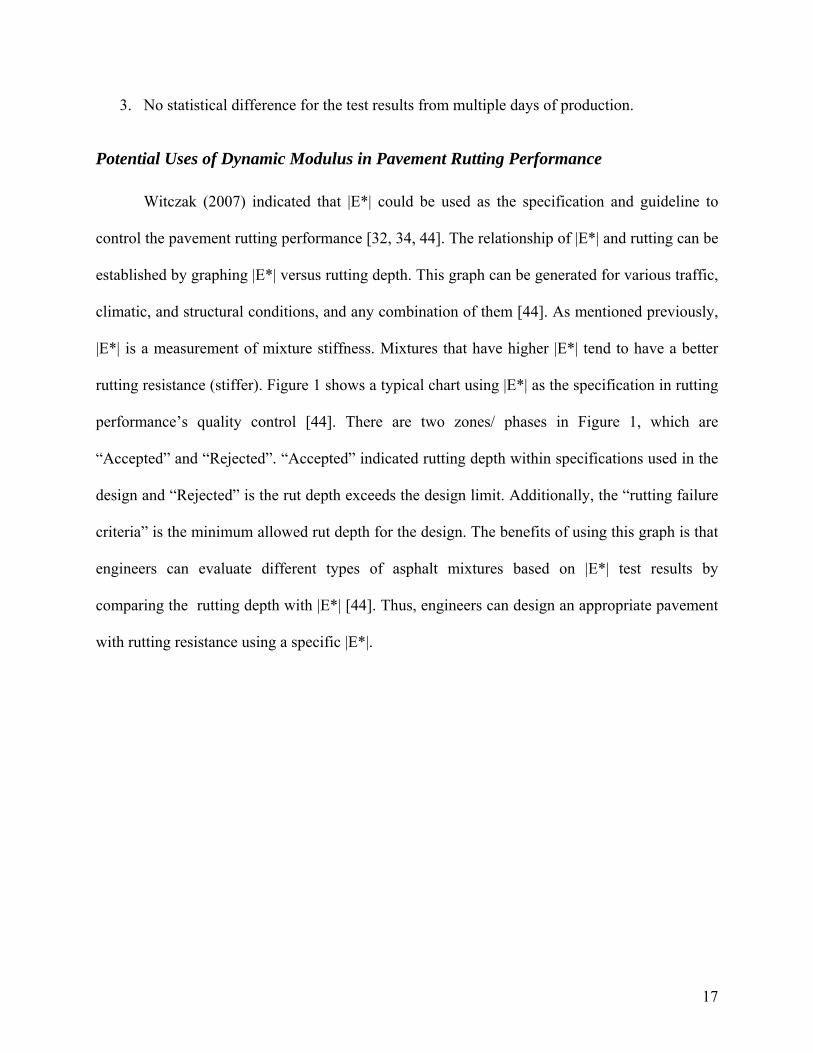
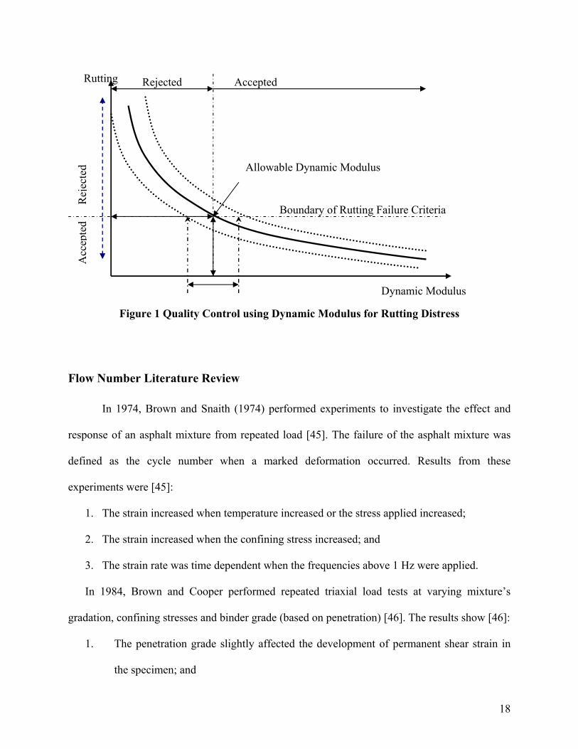
Potential Uses of Dynamic Modulus in Pavement Rutting Performance

Witczak (2007) indicated that |E*| could be used as the specification and guideline to

control the pavement rutting performance [32, 34, 44]. The relationship of |E*| and rutting can be

established by graphing |E*| versus rutting depth. This graph can be generated for various traffic,

climatic, and structural conditions, and any combination of them [44]. As mentioned previously,

|E*| is a measurement of mixture stiffness. Mixtures that have higher |E*| tend to have a better

rutting resistance (stiffer). Figure 1 shows a typical chart using |E*| as the specification in rutting

performance’s quality control [44]. There are two zones/ phases in Figure 1, which are

“Accepted” and “Rejected”. “Accepted” indicated rutting depth within specifications used in the

design and “Rejected” is the rut depth exceeds the design limit. Additionally, the “rutting failure

criteria” is the minimum allowed rut depth for the design. The benefits of using this graph is that

engineers can evaluate different types of asphalt mixtures based on |E*| test results by

comparing the rutting depth with |E*| [44]. Thus, engineers can design an appropriate pavement

with rutting resistance using a specific |E*|.

18

Figure 1 Quality Control using Dynamic Modulus for Rutting Distress

Flow Number Literature Review

In 1974, Brown and Snaith (1974) performed experiments to investigate the effect and

response of an asphalt mixture from repeated load [45]. The failure of the asphalt mixture was

defined as the cycle number when a marked deformation occurred. Results from these

experiments were [45]:

1. The strain increased when temperature increased or the stress applied increased;

2. The strain increased when the confining stress increased; and

3. The strain rate was time dependent when the frequencies above 1 Hz were applied.

In 1984, Brown and Cooper performed repeated triaxial load tests at varying mixture’s

gradation, confining stresses and binder grade (based on penetration) [46]. The results show [46]:

1. The penetration grade slightly affected the development of permanent shear strain in

the specimen; and

Rej

ecte

d A

ccep

ted

Rutting

Boundary of Rutting Failure Criteria

Rejected Accepted

Allowable Dynamic Modulus

Dynamic Modulus

19

2. The gradation of the mixture affected the shear strain significantly. Higher shear strain

was found under fewer load cycles for gap-graded mixtures.

In 1995, Mallick et al. (1995) investigated the effects of air voids on repeated loading test

[47]. These tests were correlating to field rutting performance with the measured strain from a

repeated load test. The tests were performed at 60°C (an average of high pavement temperature

in the United States) based on the ASTM D4123-82 standard specification. Various loads and

confining pressures were used in the test. A logarithmic relationship was found between air voids

and permanent strain when a 826.8kPa normal pressure and a 137.8kPa confining pressure were

applied. The results also indicated that samples at or below 3.0% air void level underwent

dilation and samples with greater than 3.0% air voids underwent consolidation. The authors

indicated samples undergoing dilation reflected the field performance (e.g. shoving). Mallick et

al. (1995) also analyzed the rutting behavior using the field procured samples under the same

condition (e.g. 826.8kPa normal pressure and a 137.8kPa confining pressure). A strong

correlation was found between permanent strain and rutting rate and it was concluded the

dynamic confined testing could used to identify rutting performance of a mixture.

In 1996, Brown and Gibb (1996) investigated the roles of asphalt binder and aggregate on

permanent deformation using the uniaxial compression [48]. Different binder contents, binder

types and aggregate gradation were used. It was found that the aggregate of the mixture carry the

load to resist permanent deformation when the binder’s stiffness decreased. The repeated loading

(uniaxial compression) was better at identifying the permanent deformation because the

accumulated strains were related or similar to field conditions.

In 2002, Witczak et al. defined the cycle number where shear deformation happened as

flow number (FN) [29]. Witczak et al. (2002) indicated FN can be used to identify the quality of

20

asphalt mixtures in terms of rutting resistance. Kaloush and Witczak (2002) indicated that the

repeated load test can be used for different applications [49]. They found out that confined

testing had a good relationship with field results. In addition, the axial or radial strain could be

used for Flow Time (FT) measurement. It was reported that results obtained from both of the FT

and FN testing were comparable [34, 44, 50].

Further investigation of flow number testing was performed by Zhou and Scullion (2003)

[13]. Similar to Witczak et al. (2002), Zhou and Scullion (2003) found that there was a good

correlation between field permanent deformation and FN. They also indicated that FN could be

used to compare the quality of the mixtures in terms of rutting performance.

A study of effects of binder content on FN was performed by Mohammad et al (2005) [43,

51]. Different binder contents were used by the author during the FN test. It was found that the FN

was not as sensitive as dynamic modulus test for the changes in asphalt content based on

statistical analysis.

21

CHAPTER 3: EXPERIMENTAL DESIGN

Asphalt mixture preparations and performance testing were completed by using the

Superpave Mix Design Specification, SP-2 [52]. A total of three different mix sizes (mixture

nominal maximum aggregate size) ranging from size 3 to 5 (19.00mm to 9.5mm) were chosen in

this project. Additionally, the traffic level of these design mixes were ranged from 0.3 million

equivalent single axle loads (ESALs) to 30 million ESALs.

For asphalt mixture performance testing, dynamic modulus and flow number tests were

employed. Previous findings indicated that the outcome for Flow Time (FT) testing were

comparable with flow number (FN) testing; hence, only flow number testing was considered in

this research study. Two air void levels (i.e. 4% and 7% air void levels) were used and three

replicate specimens were prepared for each test (at single temperature and single frequency), and

an average value is presented in this report. The test results were analyzed using statistical

methods which are discussed in ensuing sections. The general test flow chart is illustrated as

Figure 2.

22

Figure 2 General Flow Chart for the Experimental Design

23

Sample Collection

All the samples collected for this project are located within the State of Michigan and

were collected during summer time from year 2002 to 2005. Figure 3 shows the sample

collection area in the state of Michigan [53]. Approximately 25% of the mixtures were collected

from Upper Peninsula and the rest of the sampled mixtures were from the Lower Peninsula.

Table 3 shows the information of all the samples collected at each job site.

Figure 3 Sample Collection Areas1 in Michigan2

1 Note: “ ” indicated the location where sample were collected 2 Michigan State Map was obtained from Destination360 [20]

24

Table 3 Asphalt Mixture Information

Mix size

Traffic Level

Control Section

Job Mix Number Project Location

3 E10

47014 34519A Interchange of US-23 and M 59 (Hartland Township, Livingston County)

82062 47064A US-12 (Michigan Ave), Dearborn ---- From Firestone(Evergreen Rd) to I-94

E30 50015 46273A M 53 (From South of 28 Mile Road to North of 33 Mile Road), Macomb, Michigan

4

E1 BIO631012 53244A M-26, South Range, Houghton County (From Kearsarge Street to Tri-Mountain Ave.)

E3 MG73031 60476A

M-52 (From the Saginaw/Shiawassee County line northerly to South Branch of the Bad River in the

village of Oakley, City of St. Charles)

M74022 45440A M-90, Lexington, MI (From Babcock Road to Farr Road)

E10 82151 52804A M-53 , Detroit (From M-3 to M-102)

82062 47064A US-12 (Michigaeh .n Ave), Dearborn ---- From Firestone(Evergreen Rd) to I-94

E30 81104 47546A I-94, Dexter, MI 48130 (Entrance ramp from Baker

Road to I-94 Highway)

82143 45164A M102, Wayne and Macomb Counties (From M-53 to I-94)

5

E1 BIO631012 53244A M-26, South Range, Houghton County (From

Kearsarge Street to Tri-Mountain Ave.)

M66041 80168A M-38, Ontario-Houghton-Baraga Counties (From M-26 to Baraga Plains Road)

E3 NH27021 48344A US-2, Bessemer, MI (From Wisconsin/Michigan State Line to Eddy Street, Wakefield)

E10

MG63091 84049A

I-75BL, Auburn Hills, MI (From north of Woodward Avenue northeasterly to Opdyke Road in the city of Auburn Hills and Pontiac, Oakland

County)

63022 83707A I-96, MI (From West of Oakland County line to

Novi Road, in the cities of Wixon and Novi, Oakland County)

E30

25031 45446A I-75, MI (From South Junction of I-475 to North Junction of I-475)

58151 74577A I-75, MI (From the Ohio State line northerly to La Plaisance Road in the township of Erie, La Salle,

and Monroe, Monroe County) Note: Mix Size: Traffic Level: 3 – 19.0mm E1 – Traffic < 1 millions ESALs *ESALs: Equivalent single axle 4 – 12.5mm E3 – Traffic < 3 millions ESALs 5 – 9.5mm E10 – Traffic < 10 millions ESALs E30 – Traffic < 30 millions ESALs

25

Compaction Process

In order to compact a sample to the desired volumetric properties, there were three

procedures needed to follow: 1) measuring theoretical maximum specific gravity; 2) measuring

bulk specific gravity and determining air voids, and; 3) estimating gyration number and volume

of mixture used. These procedures will be explained in the following sections.

Rice Test (Theoretical Maximum Specific Gravity)

The Rice Test was performed to determine the theoretical maximum specific gravity

(Gmm) and density of the asphalt mixture according to ASTM D2041 [54]. 2000g of material for

each type of sample during the compacting process was used for the Rice Test and was left on

the table to dry for one day. The rice sample was then reduced to a loose sample for subsequent

testing in accordance with ASTM D2041.

Bulk Specific Gravity and Air Void

The sample’s bulk specific gravity (Gmb) and density test were performed according to

ASTM D2726 [55]. Utilizing the test results from the Rice Tests (Gmm) and the Gmb, the air voids

for each sample were determined.

Estimating Gyration Number and Mixture Volumetric Property

The desired gyration number and mixture volumetric property can be estimated by using

a trial mixture by calculating its estimated bulk specific gravity (Gmb estimated), corrected bulk

specific gravity, theoretical maximum specific gravity and air void level. In this project, a trial

1200g mixture for each mixture type was used for the 100mm diameter specimens. All of the

26

mixtures were compacted using a trial gyration number (i.e. 120 gyrations). Figure 4 shows the

pine gyratory compactor used in this project.

Figure 4 Pine Gyratory Compactor

During the compaction, height for each gyration was recorded. For each gyration, the

estimated Gmb can be calculated using the following equation [56]:

w

mx

m

mb

W

GEstimatedγγ

=_

where,

mW : Mass of Specimen (gram);

mxγ : Density of water (1 g/cm3); and

27

wγ : Volume of Sample (cm3).

The estimated Gmb was then compared with measured Gmb (Gmb calculated using the

ASTM D2726 [55]) to find out the correction factor. The correction factor can be easily

calculated using the equation below [56]:

mb

mb

GEstimatedGMeasuredFactorCorrection

___ =

The measured Gmb for each gyration can be found by multiplying the correction factor

with the estimated Gmb. Figure 5 shows a sample of estimated and corrected Gmb calculated in

this project.

0.2

0.205

0.21

0.215

0.22

0.225

0.23

0.235

0.24

0.245

0 20 40 60 80 100 120

Gyration Number

Est

imat

ed B

ulk

Spec

ific

Gra

vity

2

2.05

2.1

2.15

2.2

2.25

2.3

2.35

2.4

2.45

Bul

k Sp

ecifi

c G

ravi

ty a

fter

Cor

rect

ion

.

Estimated Bulk SpecificGravity

Bulk Specific Gravityafter Correction

Figure 5 Estimated and Corrected Bulk Specific Gravity for Trial Sample

28

The air void level for each gyration number was then calculated using the corrected Gmb.

The equation to find out the air void level is [57]:

mm

mb

GGVoidAir −= 1(%)_

Figure 6 shows a sample of air void levels calculated at each gyration number. The

gyration number was then estimated using this graph. For example, Figure 6 shows that a

gyration number 84 was needed in order to compact the sample to air void level of 4%. In

addition to this, the height of the sample could be estimated using the equation below:

weightSamplerG

HeightSamplemb

_1_ 2 ×⋅⋅=

π

where,

Sample_Height: Height of Sample (mm);

Gmb: Corrected Bulk Specific Gravity at the desired gyration number;

π: 3.142;

r: Radius of the mold (mm); and

Sample Weight: Weight of the sample (gram).

29

0.00%

2.00%

4.00%

6.00%

8.00%

10.00%

12.00%

14.00%

16.00%

18.00%

20.00%

0 20 40 60 80 100 120

Gyration Number

Air

Voi

d L

evel

(%)

Figure 6 Air Void Level for a Trial Sample

84

30

Sample Fabrication

All the compacted samples were fabricated (i.e. cutting and sawing to the desired size)

prior to the asphalt mixture performance testing. Samples were cut at a height of 150mm and a

diameter of 100mm by using a diamond masonry saw after the compaction process shown at

Figure 7. Additionally, Figure 8 shows the samples after fabrication.

After the asphalt concrete specimens were cut, all the samples’ bulk specific gravity (Gmb)

were measured again. It was notable that the drying process took approximately seven days

before thesample’s dry weight for Gmb could be measured.

Figure 7 Cutting and Coring Process

31

Figure 8 Asphalt Mixture after Cutting and Coring process

32

Dynamic Modulus Test

The dynamic modulus test was conducted according to AASHTO TP62-03 [58]. The

purpose of the Dynamic Modulus (|E*|) test is to find out the dynamic modulus, |E*| of the

asphalt mixture. |E*| is the modulus of a viscoelastic material. The dynamic modulus of a

viscoelastic test is a response developed under sinusoidal loading condition [36, 50]. In this

project, an IPC UTM 100 [59] was used for |E*| testing.

Figure 9 Dynamic Modulus Test Device (IPC UTM 100)

All the samples were attached with platens using high strength glue to the side of the

sample by using the loading platen device prior to the |E*| testing (shown in Figure 10). Samples

were then attached with three Linear Variable Differential Transformers (LVDTs) and placed in

the environment chamber. Temperatures and temperature equilibrium time used for |E*| in this

project are shown in Table 4.

33

Figure 10 Platen Loading Device

Table 4 Test Temperatures and Temperature Equilibrium Time for |E*| Test

Test Temperature (°C) Temperature Equilibrium Time from Room Temperature (Hour)

-5 12 4 8 13 6

21.3 4 39.2 7

Both top and bottom surfaces of the samples were covered with a friction reducing end

treatment cream. After that, samples were loaded into the dynamic modulus test device shown

below in Figure 11.

34

Figure 11 Dynamic Modulus Test Setup

The dynamic modulus test was started after the temperature in the transducer device

display reached the required test temperature. In addition, the frequencies used in this test were

0.1hz, 0.5hz, 1hz, 5hz, 10hz and 25hz. During the test, the recover axial strain was controlled to

be between 50 and 100 in order to obtain a precise |E*| by adjusting the positive dynamic stress

and static stress level [60]. The applied stress and the resulting recoverable axial strain response

of the specimen was measured and used to calculate the dynamic modulus and phase angle. Test

results were recorded after the test was done. Figure 12 shows the typical result from the |E*| test.

35

-120

-100

-80

-60

-40

-20

0

7.7 7.75 7.8 7.85 7.9 7.95 8 8.05

Time (s)

Mir

o-St

rain

0200400600800100012001400160018002000

Stre

ss (K

Pa)

Axial Micro-Strain #1 Axial Micro-Strain #2 Axial Micro-Strain #3 Stress

Figure 12 Sample Test Results of Dynamic Modulus Test1

1 Stress (1 curve) and strain (3 curves) in dynamic loading using 25 Hz frequency at temperature -5°C

36

Flow Number Test

The flow number test, also called dynamic creep or repeated creep test, was widely used

to determine the rutting distress as well as permanent deformation characteristic since the mid-

70s [61, 62]. This test was performed based on NCHRP Report 465 [36] and NCHRP 9-19 [18].

The test for flow number is based upon result from repeated loading and unloading of a HMA

specimen where the permanent deformation of the specimen is recorded as a function of the

number of load cycles. A sample size of 100mm diameter by 150mm height was used. Samples

were tested under unconfined condition and the duration of 0.1 second loading time followed by

0.9 second dwells(shown in Figure 13). During the test, the permanent strain at each test cycle

was recorded. The FN can be located at the minimum point of the strain rate versus cycle number

slope.

Flow Number test is a destructive test where a compressive stress was applied until the

sample failed. Figure 14 shows the failing sample after the flow number test.

Figure 13 Loading and unloading of Flow Number Test

0.1s loading

Time (Second)

Stre

ss (k

Pa)

0.9s dwell

37

Figure 14 Sample Fail after the Flow Number Test

Loading Level used in Flow Number Test

It is important to determine the magnitude of loading level used in each FN test because

this will significantly affect the FN. The NCHRP 9-19 used 69kPa for loading stress and 3kPa for

contact stress for FN unconfined test [27, 34]. This loading level was defined for the intermediate

and high test temperature in the dynamic modulus test. However, this loading level might not be

feasible for some of the mixtures (e.g. high traffic level mixture) as the samples would not

undergo tertiary flow. Based on a discussion with Dr. Williams and previous research [35, 63-

65], stress level of 600kPa (simulated from the gyratory compactor) and 30kPa for contact stress

were determined for this test.

38

Effective Rutting Temperature

Effective temperature is defined as a single temperature at which amount of permanent

deformation which occurred would be equivalent to that measured by considering each season

separately throughout the year [66]. The effective pavement temperature for rutting, which is

defined by the temperature of 20mm below the surface of the pavement, was shown as below

[64]:

Teff rutting = 30.8 – 0.12Zcr + 0.92 MAATdesign

where,

Teff rutting : Effective Rutting Temperature (°C);

Zcr : Critical depth down from pavement surface (mm);

MAATdesign : Mean annual air temperature (°C);

and,

MAATdesign : MAATAverage + KασMAAT

where,

MAATAverage: Average annual air temperature;

Kα : Appropriate reliability level of 90%; and

σMAAT: Standard deviation of distribution of MAAT for site location.

The critical depth, Zcr, is 20mm in this case. The MAATaverage were collected from the

Michigan State Climatology Office from stations around the entire State of Michigan. In this

report, the calculation of σMAAT used was different due to the climate in Michigan. Traditional

σMAATwas calculated using historical MAATAverage. Michigan climate was known to have a huge

39

temperature difference between winter and summer period (about a 72ºC difference). Hence,

using the traditional σMAAT calculation was not appropriate. In this report, the σMAAT was

calculated based on historical MAATAverage from each month in a year. The effective temperature

was calculated at each Michigan Department of Transportation region (shown in Figure 15):

Superior Region, North Region, Grand Region, Bay Region, Southwest Region, University

Region and Metro Region [67]. An average of Teff rutting, 45°C computed from each region was

used as the FN test temperature.

Figure 15 MAAT Average and MAAT Standard Deviation in Michigan1

1 Map taken from MDOT Website

Tavg=4.81C, Tstdev=10.44C







40

CHAPTER 4: TEST RESULTS AND FIELD INFORMATION

Introduction

The laboratory tests (including flow number and dynamic modulus tests) were conducted

at Michigan Technological University. Table 5 shows the descriptor for the sample used in this

study. Dynamic modulus (|E*|) for different mixtures were tested using the Universal Testing

Machine (UTM). Temperatures used in |E*| test were -5°C, 4°C, 13°C, 21.3°C and 39.2°C, and

frequencies used were 0.1hz, 0.5hz, 1hz, 5hz, 10hz and 25hz. The air void level used in this

project was 4% and 7%. One analysis file was obtained for each load frequency and temperature.

A total of three to six replicate specimens were tested for each mixture type. Results from |E*|

test were plotted and are shown in the following section.

The field information obtained included rutting performance, traffic data and pavement

structure. The field rutting performance and pavement structure were provided by Michigan

Department of Transportation (MDOT) [68] and the traffic information were obtained from

MDOT Traffic Monitoring Information System (MDOT TMIS). All this information is shown in

the following section as well.

41

Table 5 Descriptors for each Asphalt Mixture

Mix size Traffic Level Job Mix Number Descriptors

3 E10 34519A 3E10I 47064A 3E0 II

E30 46273A 3E30 I

4

E1 53244A 4E1 I

E3 60476A 4E3 I 45440A 4E3 II

E10 52804A 4E10 I E30 45164A 4E30 II

5

E1 53244A 5E1 I 80168A 5E1 II

E3 48344A 5E3 I

E10 84049A 5E10 I 83707A 5E10 II

E30 45446A 5E30 I 74577A 5E30 II

Dynamic Modulus Test Results

As mentioned previously, the dynamic modulus test was conducted according to

AASHTO TP62-03 [58]. An IPC UTM-100 machine [59] was used for the |E*| testing. The

temperatures used were -5°C, 4°C, 13°C, 21.3°C and 39.2°C. The frequencies used in this testing

were 0.1hz, 0.5hz, 1hz, 5hz, 10hz, and 25hz. A total of three replicates samples were tested for

each of the fifteen mixtures at each temperature and loading frequency each single test. The

recoverable axial micro-strain in this test was controlled within 50 and 100 micro strain so that

the material was in the viscoelastic range [60]. Results of the dynamic modulus test are shown in

Figure 16 to Figure 25.

42

Figure 16 Dynamic Modulus for 4% Air Void Level at -5°C

4E30 II

4E10 I

5E30 I 5E10 I 3E30 I

4E3 II 3E10 II

4E3 I 5E10 II 5E30 II 5E1 I 5E1 II 5E3 I

3E10 I

4E1

43

Figure 17 Dynamic Modulus for 7% Air Void Level at -5°C

5E30 II 4E10 I 3E30 I 4E30 II 5E10 I 5E10 II 5E30 II 3E10 I 4E3 II

3E10 II 4E3 I

5E3 I 5E1 I 5E1 II 4E1

44

Figure 18 Dynamic Modulus for 4% Air Void Level at 4°C

4E30 II 5E30 I 5E10 I

4E3 II

4E10 I 3E10 I 3E30 I 5E30 II 3E10 II 5E10 II

5E1 II 5E3 I 4E1 5E1 I 4E3 I

45


4E30 II 5E30 I 5E30 II 5E30 II 4E10 I 3E10 I 5E10 I 3E10 I 4E3 I

4E1 4E3 II 3E30 I

5E1 I

5E1 II 5E3 I

46


4E30 I 4E30 II 3E30 I 3E10 I 5E10 II 5E10 I 5E30 II 3E10 II 4E10 II 4E3 II 4E1 4E3 1 5E3 I 5E1 I 5E1 II

47


4E30 II 5E30 I 3E30 I 4E10 I

5E10 II 3E10 I

5E30 II 5E10 I 4E3 I 3E10 II 5E10 II 5E1 I 4E1 5E3 I 5E1 II

48

Figure 22 Dynamic Modulus for 4% Air Void Level at 21.3°C

4E30 II 5E30 I

5E30 II 4E10 I

3E30 I

3E10 II 5E10 II 4E3 II 5E10 I 3E10 II 4E3 I 4E1 I 5E3 I 5E1 I 5E1 II

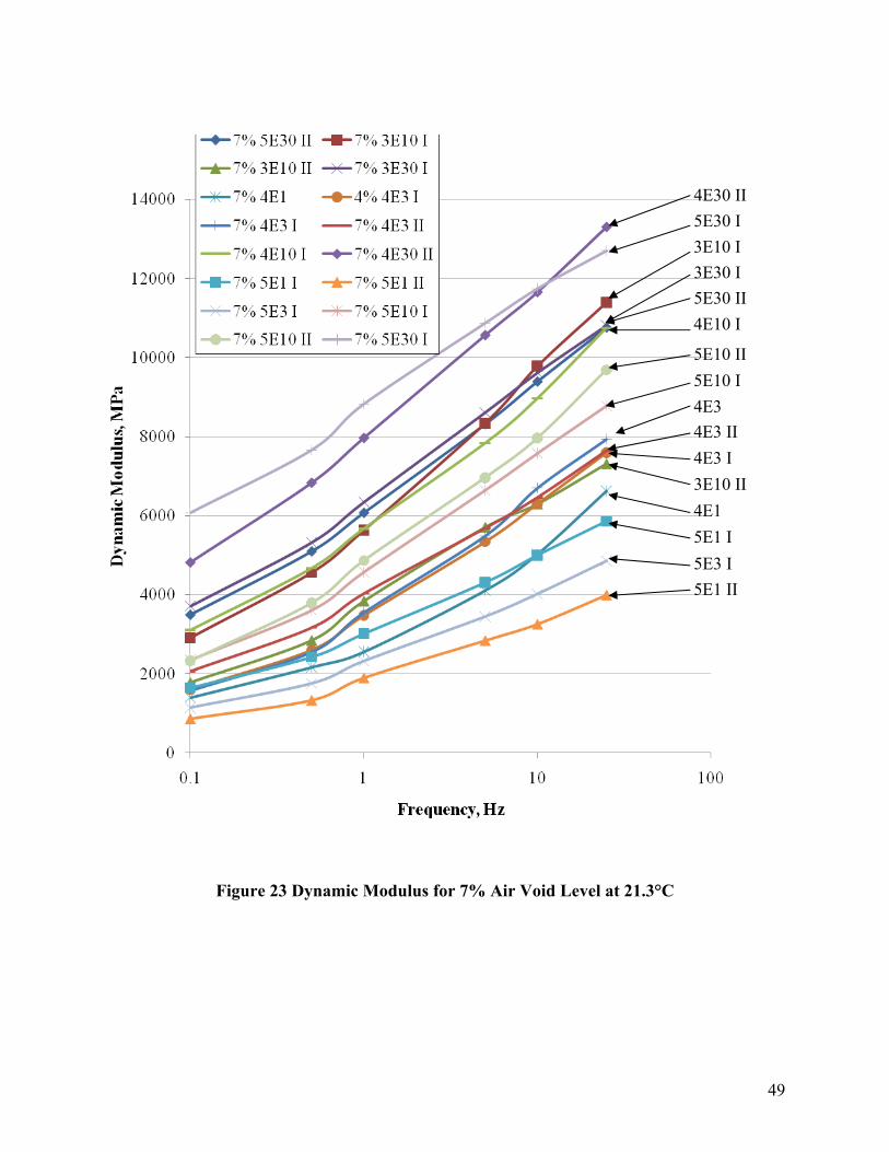
49


3E10 II

4E30 II

5E10 I

5E30 I 3E10 I 3E30 I

4E10 I 5E30 II

5E10 II

4E3 4E3 II 4E3 I

4E1 5E1 I 5E3 I 5E1 II

50


4E30 II 5E30 I 3E30 I 4E10 I 3E10 II 5E30 II 5E10 II 5E10 I 4E3 II 3E10 II 4E3 I 4E1 5E3 I 5E1 I 5E1 II

51


5E30 I

4E30 II

4E10 I 5E30 II 3E30 I 5E10 II 5E10 I

3E10 I

4E3 I 4E3 II 3E10 II

5E3 I

5E1 I

4E1

5E1 II

52

Flow Number Test Results

The flow number test was conducted according to NCHRP Report 465[66] with unconfined

testing. During the flow number testing, some of the mixtures did not undergo tertiary flow

because these mixtures have a much higher stiffness (high modulus). A simple approach to

determine the flow number of asphalt mixtures during a dynamic creep test was used in this

project. The result of the flow number testing is shown in Table 6.

Table 6 Average Flow Number Measured using Stepwise Approach

Descriptors Test Temperature

4% Air Void Level 7% Air Void Level

Average Standard Deviation Average Standard

Deviation

3E10I 45 3029 330 1759 92 3E0 II 45 1731 308 725 69 3E30 I 45 13099 3279 4829 777 4E1 I 45 320 35 134 11 4E3 I 39.2 No FN No FN No FN No FN 4E3 II 45 13995 3093 1710 - 4E10 I 45 11136 420 - - 4E30 II - - - - - 5E1 I 45 468 327 346 - 5E1 II 45 450 17 251 111 5E3 I 45 439 193 220 50 5E10 I 39.2 No FN No FN No FN No FN 5E10 II 39.2 No FN No FN No FN No FN 5E30 I 45 No FN No FN No FN No FN 5E30 II 45 No FN No FN No FN No FN

53

Field Rutting Results

The field rutting performance was provided by the Michigan Department of

Transportation (MDOT) [68]. Field data for all HMA pavements with up to seven years in

service were collected in this study. An average rutting value from left and right lanes was used

in this study. The summary of the field rutting results are shown in Table 7.

Table 7 Field Rutting Results

Mix Name/ Type Job Mix Number Year Average Rut Value

(left/right), inch

3E10 I 34519A 2003 0.000 2005 0.035 2007 0.170

3E10 II 47064A 2003 0.000 2007 0.245

3E30 I 46273A 2002 0.000 2005 0.080 2007 0.169

4E3 I 60476A 2005 0.000 2006 0.136

4E3 II 45440A

2000 0.000 2002 0.218 2004 0.067 2006 0.207

4E10 I 52804A 2003 0.000 2005 0.057 2007 0.114

4E30 II 45164A

1999 0.000 2000 0.057 2002 0.105 2004 0.058 2006 0.275

5E1 II 53244A 2005 0.000

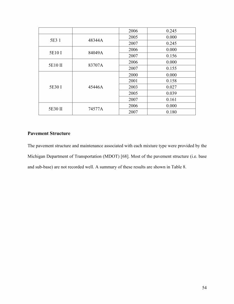
54

2006 0.245

5E3 1 48344A 2005 0.000 2007 0.245

5E10 I 84049A 2006 0.000 2007 0.156

5E10 II 83707A 2006 0.000 2007 0.155

5E30 I 45446A

2000 0.000 2001 0.158 2003 0.027 2005 0.039 2007 0.161

5E30 II 74577A 2006 0.000 2007 0.180

Pavement Structure

The pavement structure and maintenance associated with each mixture type were provided by the

Michigan Department of Transportation (MDOT) [68]. Most of the pavement structure (i.e. base

and sub-base) are not recorded well. A summary of these results are shown in Table 8.

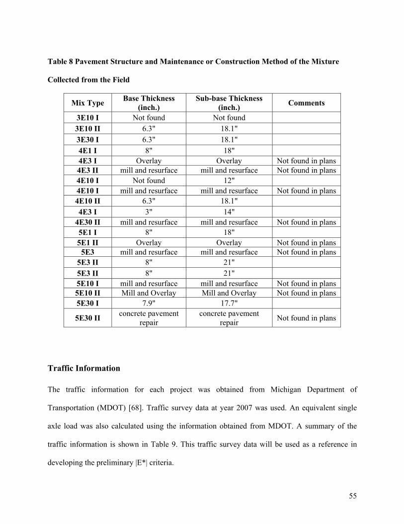
55

Table 8 Pavement Structure and Maintenance or Construction Method of the Mixture

Collected from the Field

Mix Type Base Thickness (inch.)

Sub-base Thickness (inch.) Comments

3E10 I Not found Not found 3E10 II 6.3" 18.1" 3E30 I 6.3" 18.1" 4E1 I 8" 18" 4E3 I Overlay Overlay Not found in plans 4E3 II mill and resurface mill and resurface Not found in plans 4E10 I Not found 12" 4E10 I mill and resurface mill and resurface Not found in plans 4E10 II 6.3" 18.1" 4E3 I 3" 14"

4E30 II mill and resurface mill and resurface Not found in plans 5E1 I 8" 18" 5E1 II Overlay Overlay Not found in plans

5E3 mill and resurface mill and resurface Not found in plans 5E3 II 8" 21" 5E3 II 8" 21" 5E10 I mill and resurface mill and resurface Not found in plans 5E10 II Mill and Overlay Mill and Overlay Not found in plans 5E30 I 7.9" 17.7" 5E30 II concrete pavement

repair concrete pavement

repair Not found in plans

Traffic Information

The traffic information for each project was obtained from Michigan Department of

Transportation (MDOT) [68]. Traffic survey data at year 2007 was used. An equivalent single

axle load was also calculated using the information obtained from MDOT. A summary of the

traffic information is shown in Table 9. This traffic survey data will be used as a reference in

developing the preliminary |E*| criteria.

56

Table 9 Traffic Information for each Mixture

Mix Name/ Type Project Year AADT1

Number of Equivalence

Truck ESALs2

3E10 I M-59 Brighton 2003 47933

2927 4.05E+05 2005 49213 2007 48298

3E10 II Michigan Ave, Dearborn

2003 23761 522 9.59E+04

2007 25081

3E30 I Vandyke, Detroit 2002 24706

1322 2.03E+05 2005 27471 2007 31289

4E3 I Lansing, MI 2005 8058

248 3.27E+04 2006 6805

4E3 II Lexington

2000 7594

111 1.71E+04 2002 7594 2004 8206 2006 6805

4E10 I M-53 Detroit 2003 16701

859 1.44E+05 2005 17147 2007 15266

4E10 II Michigan Ave 2003 23761

522 9.59E+04 2007 24617

4E30 I I-94 Ann Arbor (SMA)

2000 51601

6296 8.44E+05 2001 5224 2003 54460 2005 49256 2007 54841

4E30 II 8 Mile Road

1999 58143

5722 7.80E+05 2000 57070 2002 66062 2004 70426 2006 60279

5E1 II M-38 2005 586

31 4.91E+03 2006 698

1 Annual Average Daily Traffic 2 Equivalent single axle loads

57

5E3 1 Bessemer, MI 2005 49213

279 3.72E+04 2007 50170

5E10 I Auburn Hills 2006 16636

691 9.63E+04 2007 16837

5E10 II x, OH 2006 64553

718 1.30E+05 2007 66782

5E30 I I-75 Clarkston

2000 62421

2836 4.06E+05 2001 65781 2003 63873 2005 60055 2007 60858

5E30 II I-75 Toledo 2006 62117

3330 4.94E+05 2007 60937

58

CHAPTER 5: ANALYSIS AND DISCUSSIONS

Introduction

Currently, the analysis of the pavement structure was not used in this project due to the

limited information obtained. Hence, the analysis and discussion of results will fall into five

main categories, they are:

1. Analysis and discussions of dynamic modulus test results;

2. Evaluation of field rutting performance;

3. Evaluation of traffic data;

4. Analysis of field rutting performance over various traffic levels; and

5. Development of specifications for dynamic modulus.

For the first category, the dynamic modulus was analyzed using different methods

including recommendations from the literature reviews (E*/sinϕ, E*, different traffic levels, etc).

The main objective is to determine appropriate criteria from dynamic modulus testing that can be

used in developing the specification for dynamic modulus. The second and third categories were

analyzed to determine an appropriate parameter for the comparison of the field rutting

performance, traffic levels and dynamic modulus. The fourth category is to analyze the quality of

the mixture in the field based on the mixture design. Finally, the fifth category is the most

important part in the entire report, which is to develop the criteria of the dynamic modulus based

on current results and information obtained.

59

Analysis and Discussions of Dynamic Modulus Test Results

Past research work indicated that there were two kinds of parameters from the dynamic modulus

test that could be used to evaluate the pavement rutting performance: |E*| and |E*|/ sinϕ. In this

study, these two parameters were evaluated. Figure 26 and Figure 27 show the |E*| tested at

different traffic levels. The nominal maximum aggregate sizes were 19.0mm (designated mix

size “3” in the Michigan DOT specification), 12.5mm (mix size 4), and 9.5mm (mix size 5), as

mentioned in the previous section. For each frequency, an average of the |E*| values at the same

traffic level over three different mix sizes (size 3, 4 and 5) was plotted. Similarly, |E*|/sinϕ at

various traffic levels are plotted and shown in Figure 28 and Figure 29. As expected, the

dynamic modulus values are increased when the design traffic level increased. This also

indicated that mixtures with higher modulus values are able to resist more rutting or allow higher

traffic volumes. For |E*|/sinϕ, it is noticeable that this trend (traffic level increased, |E*|/sinϕ

increased) is not apparent at the 0.1 hertz and 0.5 hertz frequencies for the test results at 39.2°C.

Based on the current dynamic modulus test results, |E*| alone was found to be more

suitable in developing the specification because it is more consistent in terms of traffic level

when compared to |E*|/sinϕ.

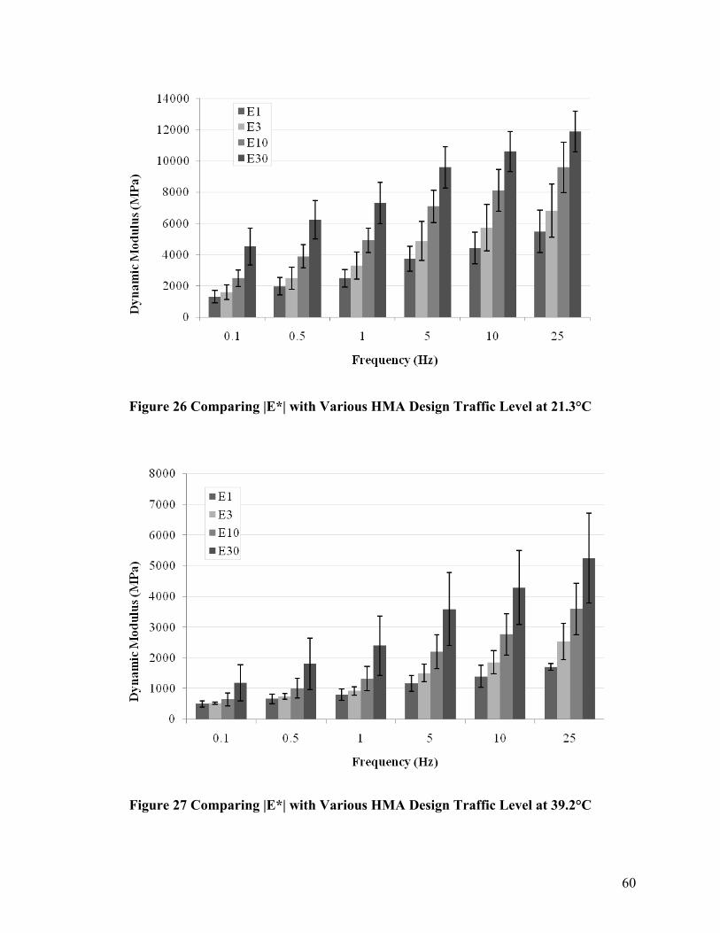
60

Figure 26 Comparing |E*| with Various HMA Design Traffic Level at 21.3°C

Figure 27 Comparing |E*| with Various HMA Design Traffic Level at 39.2°C

61

Figure 28 Comparing |E*|/sinδ with Various HMA Design Traffic Level at 21.3°C

Figure 29 Comparing |E*|/sinδ with Various HMA Design Traffic Level at 39.2°C

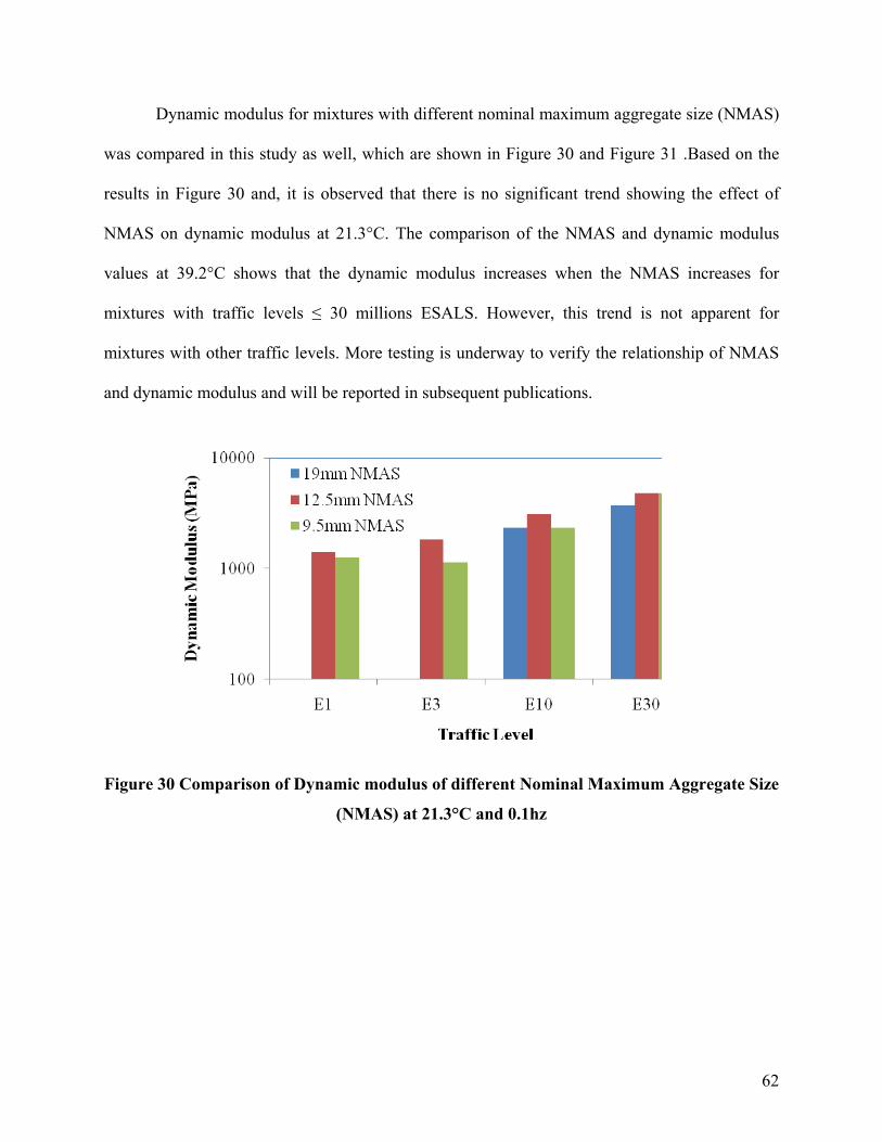
62

Dynamic modulus for mixtures with different nominal maximum aggregate size (NMAS)

was compared in this study as well, which are shown in Figure 30 and Figure 31 .Based on the

results in Figure 30 and, it is observed that there is no significant trend showing the effect of

NMAS on dynamic modulus at 21.3°C. The comparison of the NMAS and dynamic modulus

values at 39.2°C shows that the dynamic modulus increases when the NMAS increases for

mixtures with traffic levels ≤ 30 millions ESALS. However, this trend is not apparent for

mixtures with other traffic levels. More testing is underway to verify the relationship of NMAS

and dynamic modulus and will be reported in subsequent publications.

Figure 30 Comparison of Dynamic modulus of different Nominal Maximum Aggregate Size

(NMAS) at 21.3°C and 0.1hz

63

Figure 31 Comparison of Dynamic modulus of different Nominal Maximum Aggregate Size

(NMAS) at 39.2°C and 0.1hz

64

Analysis of Flow Number Results

In this section, the flow number measurement using Stepwise approach was compared with the

Three-stage Model [62], the mathematical product of Creep Stiffness and Cycles versus Cycles

method [69] and FNest method [70]. All the flow number data were compared and shown in

Figure 32 to Figure 35. It can be observed that the stepwise method has flow number

measurement similar to the Three-Stage and the mathematical product of Creep Stiffness and

Cycles versus Cycles methods. The correlation between the stepwise method and these two

methods was excellent, by showing the R-square ≥0.98. The flow number measured from the

stepwise method was significantly higher than the FNest method. As mentioned previously,

Archilla et. al. [70] recommended that a more stable method that is less dependent on operator

input and interoperation was needed for FNest Method.

In this study, the proposed stepwise method was compared with the traditional method.

Figure 35 shows the comparison results. It was observed the correlation between stepwise and

traditional method was fair (R-square=0.5969). It is worth noting that the traditional method may

provide a misleading flow number due to some deceptive points as previously mentioned.

Even though the flow number can be well-defined by all the methods discussed, the

stepwise method was determined to be more practical and easier to compute.

65

Figure 32 Comparisons of Stepwise and Three-Stage Methods

66

Figure 33 Comparison of Stepwise and Creep Stiffness times Cycles versus Cycles Methods

67

Figure 34 Comparison of Stepwise and FNest Methods

68

Figure 35 Comparison of Stepwise and Traditional Methods

69

Relationship between Deformation Rate and Stepwise Flow Number

Previous studies indicated that the rate of deformation (slope of the secondary flow) in

the dynamic creep test correlated well with permanent deformation [71]. In addition, the rate of

deformation was an important factor for determining the final flow number [72]. In this study,

flow number was computed using the stepwise method at 39.2°C and 45°C. Also, air void levels

ranging from 4% to 7% were used. Figure 36 shows the comparison between the stepwise flow

number and rate of deformation for all mixtures tested. It is notable that the rate of deformation

was computed using the stepwise modified dataset. Observations of Figure 36 indicate that an

excellent relationship was found when a regression analysis using the equation below was

employed:

Flow Number =

Where “a” and “b” are regression coefficients and FNSlope is the rate of deformation.

Since the equation above was built using different temperatures and air void levels, an R-square

of 0.96 showed that this equation is able to compute flow number of an asphalt mixture using the

rate of deformation tested at any temperature and any air void level. In this case, “a” and “b”

were calibrated and determined to be 31,753 and -1.081, respectively. Four potential benefits

were identified from using the above equation:

1) Flow number can be computed for the test that does not undergo tertiary flow

2) The computation of effective rutting temperature can be neglected.

3) The duration of the dynamic creep test can be shortened.

70

4) The dynamic creep test could become a non-destructive test if a lower cycle number

was used.

Figure 36 Relationship of Flow Number and Rate of Deformation at Secondary Stage

71

Evaluation of Field Rutting Performance

In this preliminary study, it was assumed that deformation of each layer (surface and leveling

layers) have an equal amount of deformation. Hence, rutting depth measured from the pavement

surface was used in this evaluation. Field data for all HMA pavements with up to seven years of

in service performance were collected in this study. The field rutting performances for all the

mixtures are plotted in a single graph and are shown in Figure 37. It is notable that the rutting of

a pavement would decrease if pavement maintenance was scheduled for that year. It was

observed that three pavements underwent maintenance –4E3I, 4E3II and 5E30I. According to

MDOT, a detail inspection is required to determine the need of warranty work when average rut

depth exceed 0.25 inches [73]. This means that pavement maintenance or warranty work is

needed when the field rutting reaches approximately 0.25 inches. It is noteworthy that this

guideline was only applied to pavement surface and not the base and sub-base layers. Based on

the field rutting performance data collected from MDOT, the pavements indicated had

maintenance between 3rd and 5th year for 4E3I; between 2nd and 4th year for 4E3II; and between

1st and 3rd year for 5E30I. For pavements that did have maintenance, it is observed that most of

the pavements had rut depths around or below 0.25 inches, except 4E3I which was 0.27 inches.

In this study, an average of total rutting per year was calculated based on the current

information. It was assumed that the field rutting increased linearly within a three-year period.

Even though this does not truly reflect the trend of rutting in the field, it was assumed that the

differences were not significant within the short period of time (up to three years). Typically,

pavement rutting performance will be collected every two years in Michigan. The rutting rate in

this study is calculated as the total rutting that occurred in the first two-year period (i.e. the

72

difference of rutting at year 3 and year 1); and if the rutting rate calculated is negative (i.e.

rutting at year 3 is lower than rutting at year 1), then the rutting rate for that two-year period was

not considered because maintenance might have occurred within that timeframe. The average

rutting rate was calculated as the average of all two-year period rutting rate for that mixture.

The theoretical pavement life for rutting resistance (known as the theoretical pavement

rutting life index) was calculated using the equation below:

Theoretical Pavement Rutting Life Index (TPRLI): Actual

Allow

RuttingRutting

where,

TPRLI: An index indicated the theoretical pavement life in the field, year;

Rutting Allow: Allowed maximum rutting, 0.25 inch; and

Rutting Actual: Actual rutting in the field per year, inch/year.

The average of pavement rutting and TPRLI for each mixture is shown in Table 10. It is

notable that mixtures with larger TPRLI indicated the pavement will last longer in the field. This

information will be used for different traffic levels and in the development of dynamic modulus

specification criteria.

73

Figure 37 Field Rutting Data (Maintenance occurred when rutting reached approximately

0.25 in.)

74

Table 10 Field Rutting Performance and Mixture’s Theoretical Pavement Rutting Life

Index

Mix Name/ Type Year

Average Rut Value (left/right),

inch

Average Rut Value (left/right), inch/year TPRLI

3E10 I 2003 0.000

0.0425 5.8824 2005 0.035 2007 0.170

3E10 II 2003 0.000

0.0613 4.0816 2007 0.245

3E30 I 2002 0.000

0.0356 7.0221 2005 0.080 2007 0.169

4E3 I 2005 0.000

0.1363 1.8337 2006 0.136

4E3 II

2000 0.000

0.0894 2.7980 2002 0.218 2004 0.067 2006 0.207

4E10 I 2003 0.000

0.0286 8.7500 2005 0.057 2007 0.114

4E10 II 2003 0.000

0.0613 4.0816 2007 0.245

4E30 I

2000 0.000

0.1049 2.3838 2001 0.210 2003 0.096 2005 0.116 2007 0.305

4E30 II

1999 0.000

0.0632 3.9587 2000 0.057 2002 0.105 2004 0.058 2006 0.275

5E1 II 2005 0

0.2450 1.0204 2006 0.245

5E3 1 2005 0.000

0.1225 2.0408 2007 0.245

75

5E10 I 2006 0.000

0.1564 1.5988 2007 0.156

5E10 II 2006 0.000

0.1547 1.6158 2007 0.155

5E30 I

2000 0

0.0751 3.3308 2001 0.158 2003 0.027 2005 0.039 2007 0.161

5E30 II 2006 0

0.1803 1.3869 2007 0.180

Evaluation of Traffic Data

In this project, equivalent single axle loads (ESALs) for each mixture were calculated

based on the traffic information obtained from the MDOT TMIS. The traffic level for each

mixture type is shown in Table 11. It is assumed that the pavement will fail and need

maintenance when the accumulated field traffic reaches the designed traffic level. The design

pavement life (known as design life index) can be calculated using following equation:

Design Life Index: Actual

Allow

ESALsESALs

where,

Design Life Index: An index indicated the theoretical pavement life based on design, year;

ESALs Allow: Designed asphalt mixture’s traffic level, ESALs; and

ESALs Actual: Actual traffic level in that area, ESALs/year.

The designed life index of each mixture is shown in Table 12. It is notable that the larger value in design life index indicated the pavement will last

longer based on the design. This information will be used as a reference when developing the

trial dynamic modulus and flow number specification.

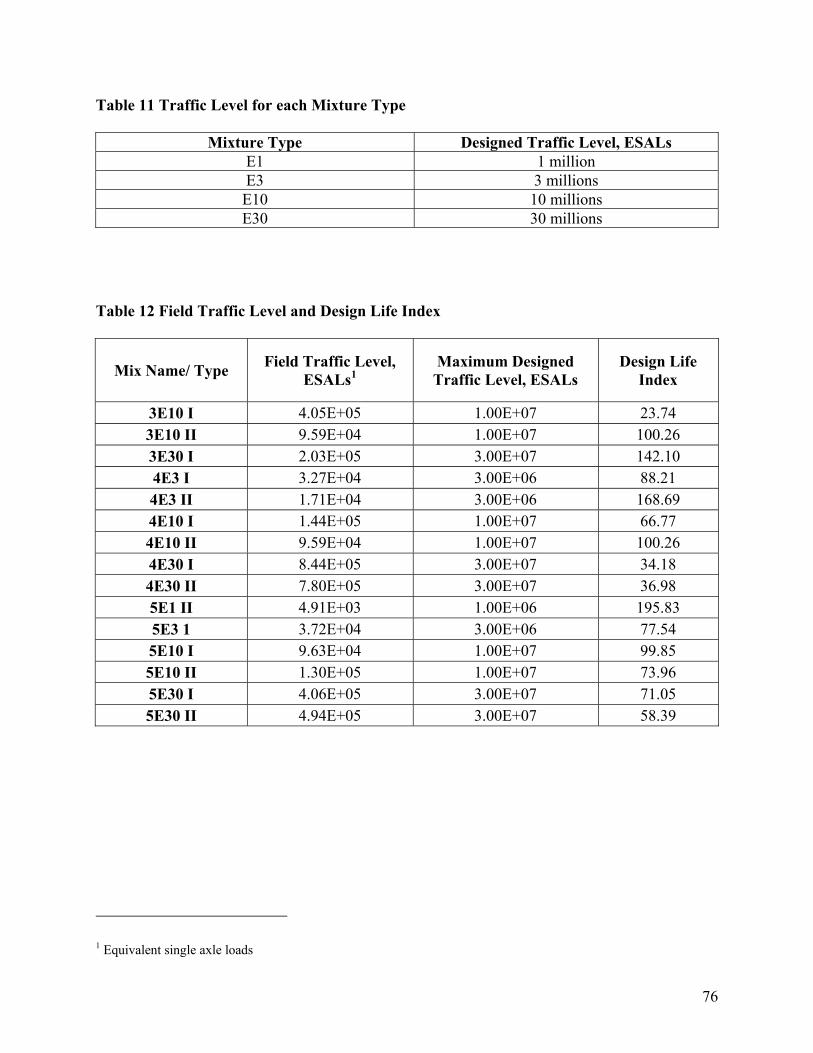
76

Table 11 Traffic Level for each Mixture Type

Mixture Type Designed Traffic Level, ESALs E1 1 million E3 3 millions E10 10 millions E30 30 millions

Table 12 Field Traffic Level and Design Life Index

Mix Name/ Type Field Traffic Level, ESALs1

Maximum Designed Traffic Level, ESALs

Design Life Index

3E10 I 4.05E+05 1.00E+07 23.74 3E10 II 9.59E+04 1.00E+07 100.26 3E30 I 2.03E+05 3.00E+07 142.10 4E3 I 3.27E+04 3.00E+06 88.21 4E3 II 1.71E+04 3.00E+06 168.69 4E10 I 1.44E+05 1.00E+07 66.77 4E10 II 9.59E+04 1.00E+07 100.26 4E30 I 8.44E+05 3.00E+07 34.18 4E30 II 7.80E+05 3.00E+07 36.98 5E1 II 4.91E+03 1.00E+06 195.83 5E3 1 3.72E+04 3.00E+06 77.54 5E10 I 9.63E+04 1.00E+07 99.85 5E10 II 1.30E+05 1.00E+07 73.96 5E30 I 4.06E+05 3.00E+07 71.05 5E30 II 4.94E+05 3.00E+07 58.39

1 Equivalent single axle loads

77

Development of Trial Dynamic Modulus Specification

In this project, the trial specification criteria of dynamic modulus were developed based on field

rutting performance and contractor warranty criteria. The rutting performance in the field was

shown in a previous section by using the term called Theoretical Pavement Rutting Life Index

(TPRLI). In this section, the Actual Life Index was used; incorporating contractor warranty

criteria and dynamic modulus test results to develop the SPT specification. The contractor

warranty for the pavement is summarized in Table 13[73].

Table 13 Contractor Warranty for Asphalt Pavement

Warranty Period Work Type

2 years Chip Seal

Micro-Surfacing Crack Treatment

3 years Non-Structural Overlays

Cold Mill and Resurfacing Hot-in-place Recycling

5 years Repair/ Rehabilitate

Reconstruction Multiple Overlays

The contractor warranty for asphalt pavement was used as the quality control and quality

assurance (QC/QA) to ensure the performance of the mixture. Based on the information from

MDOT [74], most of the mixture tested in this project were milling and re-surfacing, and only a

few mixtures are overlays. Hence, in this report, a 2 year warranty period was chosen as the one

for the design criteria in the SPT development.

The 2 year design period was compared with the TPRLI and two category mixtures were

defined as: 1) mixtures that meet the warranty, and; 2) mixtures that do not meet the warranty.

These two categories are shown in

Table 14 and Table 15, respectively.

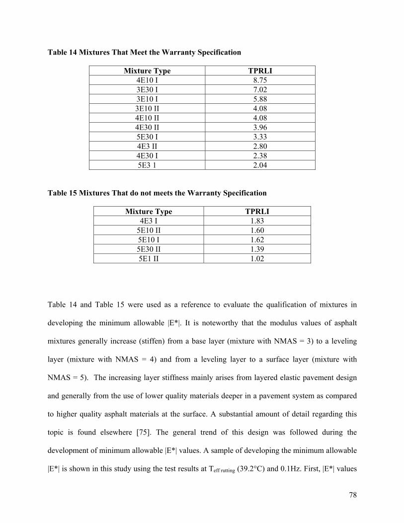
78

Table 14 Mixtures That Meet the Warranty Specification

Mixture Type TPRLI 4E10 I 8.75 3E30 I 7.02 3E10 I 5.88 3E10 II 4.08 4E10 II 4.08 4E30 II 3.96 5E30 I 3.33 4E3 II 2.80 4E30 I 2.38 5E3 1 2.04

Table 15 Mixtures That do not meets the Warranty Specification

Mixture Type TPRLI 4E3 I 1.83

5E10 II 1.60 5E10 I 1.62 5E30 II 1.39 5E1 II 1.02

Table 14 and Table 15 were used as a reference to evaluate the qualification of mixtures in

developing the minimum allowable |E*|. It is noteworthy that the modulus values of asphalt

mixtures generally increase (stiffen) from a base layer (mixture with NMAS = 3) to a leveling

layer (mixture with NMAS = 4) and from a leveling layer to a surface layer (mixture with

NMAS = 5). The increasing layer stiffness mainly arises from layered elastic pavement design

and generally from the use of lower quality materials deeper in a pavement system as compared

to higher quality asphalt materials at the surface. A substantial amount of detail regarding this

topic is found elsewhere [75]. The general trend of this design was followed during the

development of minimum allowable |E*| values. A sample of developing the minimum allowable

|E*| is shown in this study using the test results at Teff rutting (39.2°C) and 0.1Hz. First, |E*| values

79

were divided into two categories as shown in Table 16, and then the minimum allowable |E*|

was defined based on these categories. A sample procedure of selecting the minimum allowable

|E*| is shown as follows:

Scenario 1:

For mixtures with a traffic level ≤ 1 million ESALs (E1 mixture), only one mixture type is

available (5E1). In this case, the minimum |E*| criteria is justified based on |E*| value of 5E1,

and E3 mixtures. It is observed that the |E*| of 5E1 is 493MPa at 1.02 TPRLI, |E*| for 4E3 I is

558MPa at 1.83 TPRLI, and |E*| of 4E3 II is 495MPa at 2.3 TPRLI. Typically, the performance

of pavements is affected by the construction and traffic volume as well. It was suspected that

poor construction might have occurred for mixture 5E1 II because it has a low TPRLI and has

low traffic volume (based on Table 12) as well. For 4E3 I and 4E3 II, it is observed that TPRLI

for 4E3 I is lower than 4E3 II and this probably can be explained because the traffic volume for

4E3 I is much higher than 4E3 II. In order to prevent rutting for E1 mixtures, |E*| for E3

mixtures were used. In this case, minimum |E*| for E1 mixtures was justified by having the

lower E3 mixture’s |E*|, which is 495MPa for both 4E1 and 5E1.

Scenario 2:

For mixture with traffic level ≤ 3 million ESALs (E3 mixture), It is observed that |E*| for 5E3 I

is 568MPa at 2.04 TPRLI (slightly above the contractor warranty criteria). It is also observed

that 4E3 I has a similar traffic volume compared to 5E3 I, however, the TRRLI for 4E3 I is much

lower than 5E3 I. For mixtures with the same design traffic volume, it is ideal to have a similar

|E*| to resist rutting. Even though the TPRLI for 4E3 II is higher than the contractor warranty

80

criteria, the traffic volume for 4E3 II is much lower than both 4E3 I and 5E3 I. Hence for this

case, the minimum |E*| is rationalized by using |E*| of 568 MPa as the minimum limit for both

4E3 and 5E3 mixtures.

Scenario 3

For mixtures with a traffic level ≤ 10 million ESALs (E10 mixture), minimum |E*| criteria were

selected based on 3E10 I, 3E10 II, 4E10 I, 5E10 I and 5E10 II mixtures. For the 3E10 mixture

type, it is observed that the |E*| for 3E10 I is 716MPa with 5.88 TPRLI, and the |E*| for 3E10 II

is 432 with 4.08 TPRLI. It is also observed that the traffic volume for 3E10 I is much higher than

3E10 II. Based on the traffic volume, it can be explained that the |E*| for 3E10 I is much higher

than 3E10 II; and at the same time TPRLI for 3E10 I is slightly higher than 3E10 II. It is

assumed that the TPRLI is reduced when |E*| is decreased. The minimum |E*| in this case is

justified to be slightly lower than |E*| of 3E10 I. Additionally, the ideal |E*| for E10 mixtures

should be higher than E3 mixtures (compare to |E*| of 5E3). Hence, |E*| for 3E10 mixture is

selected slightly higher than E3 mixtures, and slightly lower than 3E10 I. An |E*| of 600MPa for

3E10 mixture level is selected in this case.

For the 4E10 mixture type, it is observed that 4E10 I has a high TPRLI and |E*|, and

slightly higher traffic volume compared to 3E10 II. The justification of selecting the minimum

|E*| in this case is similar to 3E10. As mentioned earlier, the stiffness of an asphalt mixture

should increase from a base layer to a leveling layer. Hence, a slightly higher criterion will be

selected for 4E30 mixtures. In this case, |E*| of 650MPa was selected.

For the 5E10 mixture type, both mixtures sampled and tested– 5E10 I and 5E10 II do not

meet the minimum warranty criteria, and they have lower traffic volume compared to both 4E10

81

I and 3E10 I. It is suspected that poor production quality could have occurred for both 5E10 I

and 5E10 II mixtures. Thus in this case, |E*| value of 650MPa, which is the same as the 4E10

criteria, is used as the minimum requirement.

Scenario 4

For mixtures with a traffic level ≤ 30 million ESALs, minimum |E*| criteria were selected based

on 3E30 I, 4E30 II, 4E10 I, 5E30 I and 5E30 II. It is observed that the |E*| for 3E30 is 806MPa

and has a high TPRLI of 7.02. Based on the traffic volume of 3E30 I, it is observed that traffic

volume for 3E30 I is much lower than 3E10 I, and the high TPRLI can be explained because

3E30 I has higher |E*| and lower traffic volume at the same time compared to 3E10 I. Ideally,

|E*| value should increase when designed traffic level increases. In this case, |E*| for 3E30 I was

selected as the minimum |E*| required. This value can be adjusted when more data becomes

available.

For the 4E30 and 5E30 mixture types, it is observed that traffic volume for 4E30 II is

much higher than 5E30 I and 5E30 II. Based on 5E30 II, it is observed that |E*| of 984MPa does

not meet the contractor warranty limit (at similar traffic volume of 5E30 I). Thus, it is apparent

that the minimum |E*| for 4E30 and 5E30 have to be higher than 984MPa. It is observed that the

TPRLI for 5E30 I is lower than 4E30 II, and |E*| of 5E30 I is higher than 4E30II, and the traffic

volume of 5E30 I is lower than 4E30 II. Hence, it is assumed that construction for 4E30 II is

better than 5E30 I. E30 mixtures are usually designed for high volume traffic (with traffic

volume up to 30 million ESALs). 4E30 II has a high traffic volume, and has TPRLI of 3.96

which it is higher than contractor warranty limit. Hence, the minimum |E*| can be justified as

82

selecting a |E*| value slightly lower than the |E*| of 4E30 II. In this case, |E*| of 1450MPa is

selected for both 4E30 and 5E30 mixture types.

Table 16 Dynamic Modulus for HMA Mixtures that meet Warranty Criteria and did not

meet Warranty Criteria at 39.2°C and 0.1Hz

Comments Mixture Type Dynamic Modulus, MPa

Mixtures that meet Warranty Criteria

3E10 I 716 3E10 II 432 3E30 I 806 4E3 II 495 4E10 I 974 4E30 II 1547 5E3 1 568 5E30 I 1855

Mixtures that not meet Warranty Criteria

4E3 I 558 5E1 II 493 5E10 I 473 5E10 II 435 5E30 II 984

No field performance Result 4E1 716 5E1 I 432

83

3 4 5

E1 495 MPa 495 MPa

E3 568 MPa 568 MPa

E10 600 MPa 650MPa 650 MPa

E30 806 MPa 1450 MPa 1450 MPa

Figure 38 Specification of Dynamic Modulus at Various Traffic Levels and Aggregate Sizes A summary of allowable |E*| values are shown in Figure 38. It is noteworthy that the

objective of this study is to try to relate the measured |E*| to the field rutting data. A more

general |E*| based criteria can only be developed when additional mixtures are tested and the

criteria validated through field performance data.

A similar method could be used to define the minimum and/or maximum allowable |E*|

at each temperature and each frequency. The sigmoidal master curve technique could also be

used to establish all these minimum and/or maximum allowable |E*| into one single curve for

various distresses including fatigue and thermal cracking. However, for brevity, the authors have

elected to limit the paper to rutting. For example, a maximum |E*| value should be specified for

thermal cracking whereas a range of |E*| values should be considered acceptable for fatigue

cracking [76]. A sample sigmoidal master curve using all the minimum and/or maximum

allowable |E*| values for a 3E10 HMA mixture was constructed using the reference temperature

of 21.3ºC and is shown in Figure 39. All other master curves, including mixtures with 4% and

7% air void level were constructed using the reference temperature of -5ºC and are shown in

Figure 40 to Figure 59. It is recommended that all the future mixtures should be tested at 3

Aggregate Size Tr

affic

Lev

el

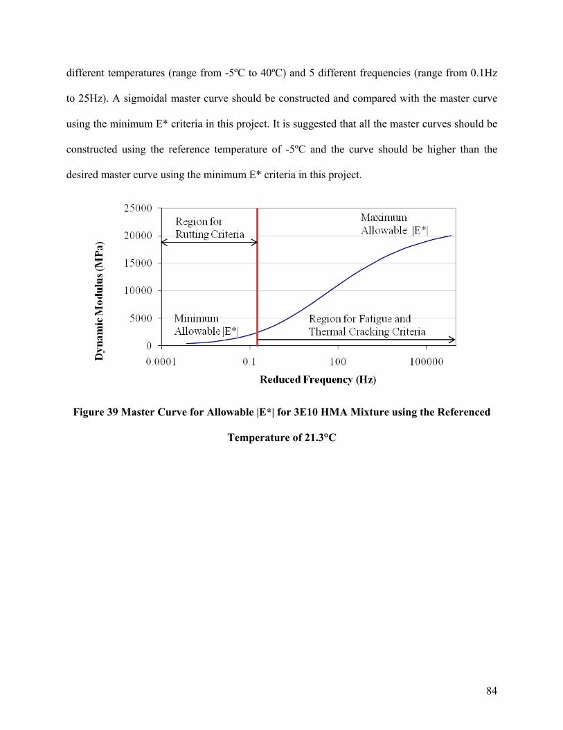
84

different temperatures (range from -5ºC to 40ºC) and 5 different frequencies (range from 0.1Hz

to 25Hz). A sigmoidal master curve should be constructed and compared with the master curve

using the minimum E* criteria in this project. It is suggested that all the master curves should be

constructed using the reference temperature of -5ºC and the curve should be higher than the

desired master curve using the minimum E* criteria in this project.

Figure 39 Master Curve for Allowable |E*| for 3E10 HMA Mixture using the Referenced

Temperature of 21.3°C

85

0

2000

4000

6000

8000

10000

12000

14000

16000

18000

20000

1E-08 1E-07 0.000001 0.00001 0.0001 0.001 0.01 0.1 1 10 100

Reduced Frequency (Hz)

Dyn

amic

Mod

ulus

(MPa

)

Figure 40 Master Curve for Minimum Required Dynamic Modulus of 3E10 at 4% Air Void Level

Note: Master Curve Parameter:

Constant Value Temperature (ºF) Log (aT) δ 4.2223 23 0.0000 ά 2.2369 39.2 -1.5239 β -3.5632 55.4 -2.8941 γ 0.6759 70.34 -4.0215 a 0.0003 102.56 -6.0082 b -0.1123 c 2.4275

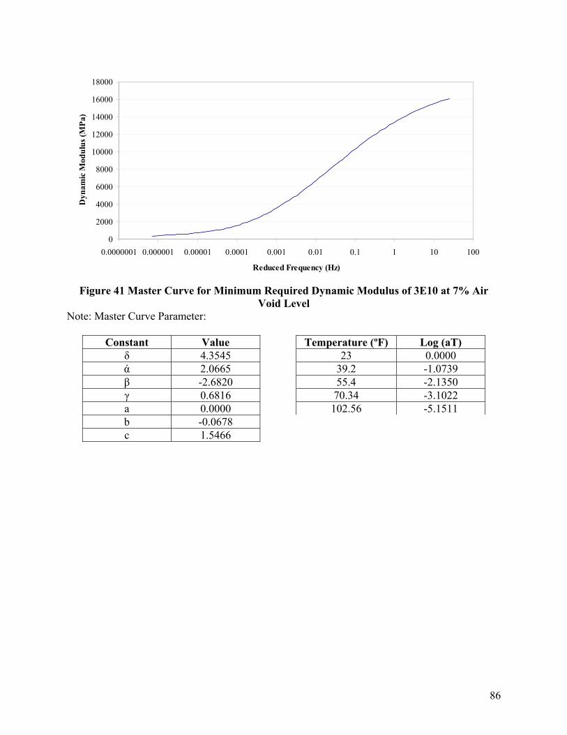
86

0

2000

4000

6000

8000

10000

12000

14000

16000

18000

0.0000001 0.000001 0.00001 0.0001 0.001 0.01 0.1 1 10 100


Dyn

amic

Mod

ulus

(MPa

)


Void Level Note: Master Curve Parameter:


87

0

2000

4000

6000

8000

10000

12000

14000

16000

18000

20000

0.000001 0.00001 0.0001 0.001 0.01 0.1 1 10 100


Dyn

amic

Mod

ulus

(MPa

)




88

0

2000

4000

6000

8000

10000

12000

14000

16000

18000

20000

0.000001 0.00001 0.0001 0.001 0.01 0.1 1 10 100


Dyn

amic

Mod

ulus

(MPa

)




89

0

2000

4000

6000

8000

10000

12000

14000

16000

18000

0.0000001 0.000001 0.00001 0.0001 0.001 0.01 0.1 1 10 100


Dyn

amic

Mod

ulus

(MPa

)

Figure 44 Master Curve for Minimum Required Dynamic Modulus of 4E1 at 4% Air Void

Level Note: Master Curve Parameter:


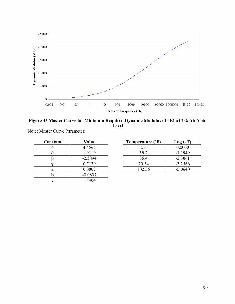
90

0

5000

10000

15000

20000

25000

0.001 0.01 0.1 1 10 100 1000 10000 100000 1000000 1E+07 1E+08


Dyn

amic

Mod

ulus

(MPa

)




91

0

5000

10000

15000

20000

25000

0.0000001 0.000001 0.00001 0.0001 0.001 0.01 0.1 1 10 100


Dyn

amic

Mod

ulus

(MPa

)




92

0

2000

4000

6000

8000

10000

12000

14000

16000

18000

1E-08 1E-07 0.000001 0.00001 0.0001 0.001 0.01 0.1 1 10 100


Dyn

amic

Mod

ulus

(MPa

)




93

0

5000

10000

15000

20000

25000

1E-08 1E-07 0.000001 0.00001 0.0001 0.001 0.01 0.1 1 10 100


Dyn

amic

Mod

ulus

(MPa

)




94

0

2000

4000

6000

8000

10000

12000

14000

16000

18000

20000

1E-08 1E-07 0.000001 0.00001 0.0001 0.001 0.01 0.1 1 10 100


Dyn

amic

Mod

ulus

(MPa

)




95

0

5000

10000

15000

20000

25000

1E-09 1E-08 1E-07 1E-06 0.00001 0.0001 0.001 0.01 0.1 1 10 100


Dyn

amic

Mod

ulus

(MPa

)



Constant Value Temperature (ºF) Log (aT) δ 3.7702 23 0.0000 ά 2.7254 39.2 -1.0598 β -4.6031 55.4 -3.6566 γ 0.5041 70.34 -6.9303 a -0.0004 102.56 -7.4831 b -0.0403 c 1.1409

96

0

5000

10000

15000

20000

25000

1E-08 1E-07 0.000001 0.00001 0.0001 0.001 0.01 0.1 1 10 100


Dyn

amic

Mod

ulus

(MPa

)




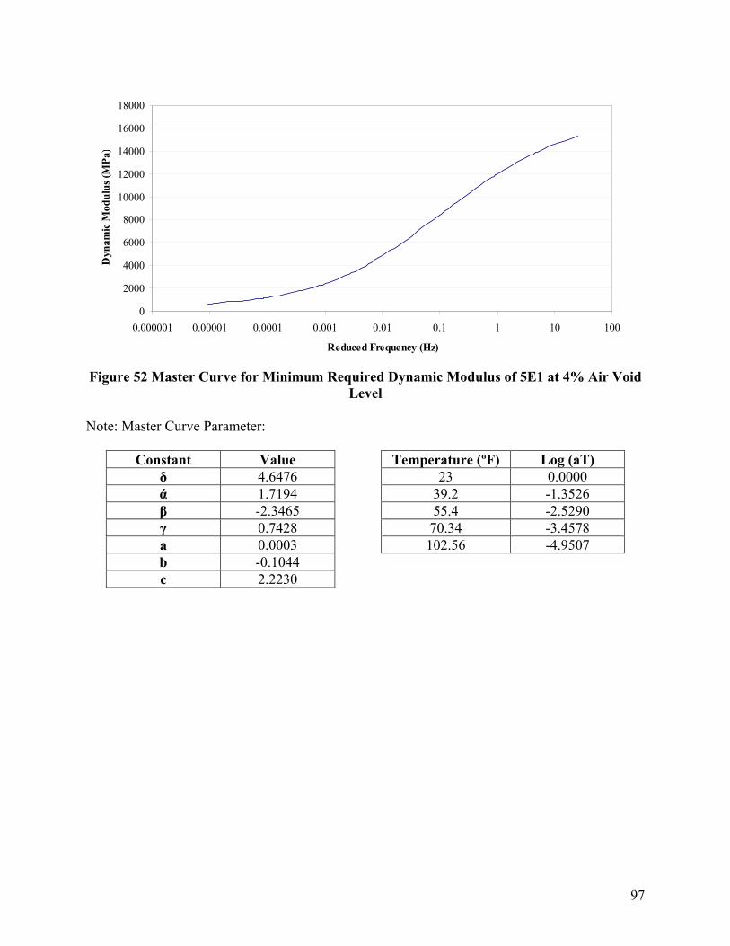
97

0

2000

4000

6000

8000

10000

12000

14000

16000

18000

0.000001 0.00001 0.0001 0.001 0.01 0.1 1 10 100


Dyn

amic

Mod

ulus

(MPa

)




98

0

2000

4000

6000

8000

10000

12000

14000

16000

0.000001 0.00001 0.0001 0.001 0.01 0.1 1 10 100


Dyn

amic

Mod

ulus

(MPa

)




99

0

2000

4000

6000

8000

10000

12000

14000

16000

18000

0.0000001 0.000001 0.00001 0.0001 0.001 0.01 0.1 1 10 100


Dyn

amic

Mod

ulus

(MPa

)




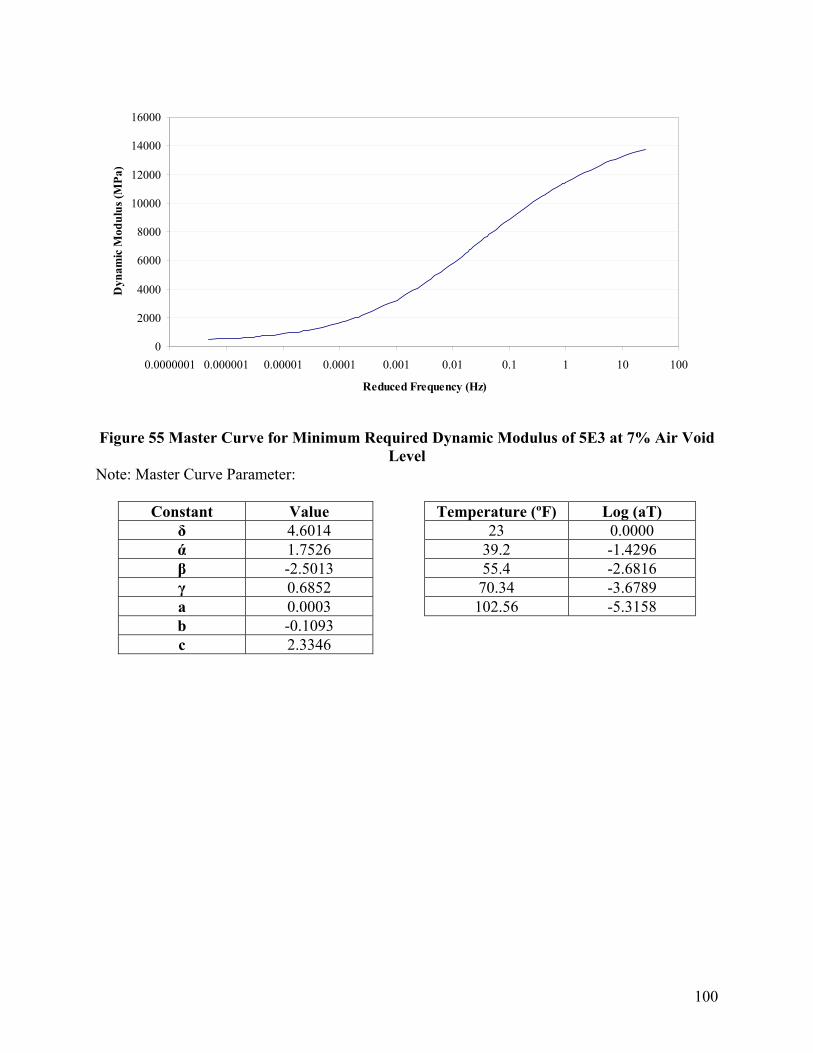
100

0

2000

4000

6000

8000

10000

12000

14000

16000

0.0000001 0.000001 0.00001 0.0001 0.001 0.01 0.1 1 10 100


Dyn

amic

Mod

ulus

(MPa

)




101

0

5000

10000

15000

20000

25000

30000

1E-08 1E-07 0.000001 0.00001 0.0001 0.001 0.01 0.1 1 10 100


Dyn

amic

Mod

ulus

(MPa

)




102

0

5000

10000

15000

20000

25000

1E-08 1E-07 0.000001 0.00001 0.0001 0.001 0.01 0.1 1 10 100


Dyn

amic

Mod

ulus

(MPa

)


Void Level



103

0

5000

10000

15000

20000

25000

30000

1E-08 1E-07 0.000001 0.00001 0.0001 0.001 0.01 0.1 1 10 100


Dyn

amic

Mod

ulus

(MPa

)




104

0

5000

10000

15000

20000

25000

1E-08 1E-07 0.000001 0.00001 0.0001 0.001 0.01 0.1 1 10 100


Dyn

amic

Mod

ulus

(MPa

)




105

Development of Trial Flow Number Specification

A similar approach in developing the specification criteria of |E*| was used in developing the

trial flow number specification. Since not all the flow number tests underwent tertiary flow, the

slope of the secondary stage during the flow number test was considered for evaluation. The

TPRLI was used in this section; incorporating contractor warranty criteria and flow number

results to develop the trial SPT specification. Table 17 and Table 18 shows the ranking of

mixtures (4% and 7% air void level) based on the flow number slope.


45°C

Descriptors

4% Air Void Level

Average Standard Deviation

5E30 I 0.0401 0.0130 4E30 II 0.2372 0.0833 4E3 II 0.3921 0.2730 3E30 I 0.9782 0.1723 4E10 I 1.3596 0.0181 3E10I 5.7866 1.2779

3E10 II 13.0318 1.4058 5E1 II 24.9128 1.5759 5E3 I 33.2563 9.2458 4E1 I 34.8156 5.2335 5E1 I 40.6422 25.3791

106


45°C

Descriptors

7% Air Void Level

Average Standard Deviation

5E30 I 0.0374 0.0108 4E30 II 0.8471 0.1429 3E30 I 3.3515 0.5221 4E3 II 4.0470 - 3E10I 12.5223 0.2037 5E1 I 20.0745 24.1038

3E10 II 38.6647 2.1836 5E3 I 64.0833 25.5252 5E1 II 66.6397 29.2130 4E1 I 89.3230 8.7479

Table 10 in the previous section was used as the reference for determining the flow

number criteria. Again, a two year warranty period was chosen as the one for the design criteria

in the SPT development. A maximum flow number slope was developed based on the Rank

index for each mixture type. Flow number was also back-calculated using the equation generated

in Figure 36, as shown below:

Flow Number = 31753

A summary of maximum flow number slope and minimum flow number criteria are

shown in Table 19 and Table 20. It is recommended that all the future mixtures should be tested

at a temperature of 45°C.

107

Table 19 Flow Number Criteria for Mixture with 4% Air Void Level

Nominal Maximum Aggregate Size Traffic Level 3 4 5

Maximum Flow

Number Slope

E1 20.00 20.00 E3 10.00 10.00 E10 5.50 5.00 5.00 E30 1.00 1.00 0.50

Minimum Flow

Number

E1 830 830 E3 1600 1600 E10 2850 3100 3100 E30 14700 14700 2860

Table 20 Flow Number Criteria for Mixture with 7% Air Void Level

Nominal Maximum Aggregate Size Traffic Level 3 4 5

Maximum Flow

Number Slope

E1 40.00 40.00 E3 35.00 35.00 E10 30.00 30.00 30.00 E30 4.00 4.00 4.00

Minimum Flow

Number

E1 430 430 E3 480 480 E10 560 560 560 E30 3900 3900 3900

108

CHAPTER 6: SUMMARY AND RECOMMENDATIONS

The Michigan Department of Transportation (MDOT) has successfully implemented the

Superpave volumetric mixture design procedure. Yet, a number of studies have shown that the

Superpave volumetric mixture design method alone is insufficient to ensure reliable mixture

performance over a wide range of traffic and climatic conditions. The development of an SPT

and corresponding performance criteria has been the focus of considerable research efforts in the

past several years. In fact, some aspects of the tests have been available for decades, such as the

dynamic modulus test of hot mix asphalt. The objectives of this study were:

1. Using the SPT, conduct a laboratory study to measure parameters including the dynamic

modulus terms (E*/sinϕ and E*) and the flow number (Fn) for typical Michigan HMA

mixtures;

2. Correlate the results of the laboratory study to field performance as they relate to flexible

pavement performance (rutting, fatigue, and low temperature cracking); and

3. Make recommendations for the SPT criteria at specific traffic levels (e.g. E3, E10, E30),

including recommendations for a draft test specification for use in Michigan.

The current report focuses intensely on rutting performance criteria. Hence, a summary

and recommendations from this preliminary SPT development project are reported as follows:

1. The effective temperature was calculated at each Michigan Department of Transportation

region: Superior Region, North Region, Grand Region, Bay Region, Southwest Region,

109

University Region and Metro Region. An average of Teff rutting, 45°C, computed from each

region, was used as the FN test temperature.

2. It was found that using the traditional σMAAT calculation was not appropriate for the state

of Michigan. In this report, the σMAAT was calculated based on historical MAATAverage

from each month in a year.

3. Dynamic modulus values within the range of 50-100 micro-strains are lower as compared

to 100-150 micro-strain level. The literature reviews suggested that the strain level should

be controlled between 50 to 100 micro-strains to maintain the material’s viscoelastic

behavior.

4. Based on the test results, the dynamic modulus increases with a decrease in asphalt

content, a decrease in air voids, and a decrease in compaction effort. The dynamic

modulus increases when the temperature is decreased and the frequency is increased.

Additionally, the dynamic modulus increases when the asphalt viscosity increases.

5. The dynamic modulus is higher at a higher design traffic level. This indicates that a

mixture with a higher modulus is able to better resist rutting than a mixture with a lower

modulus value.

6. Based on the dynamic modulus test results, |E*| alone was found to be more suitable in

developing the draft specification.

7. In this project, the draft specifications for dynamic modulus were developed based on

field rutting performance and contractor warranty criteria. A 2-year warranty period was

chosen as the design criteria in the SPT development. The minimum dynamic modulus

values were selected at each frequency at each temperature based on the test results

developed for this study. The sigmoidal master curve technique was used to develop

110

minimum criteria for a single master curve criteria for the various mix sizes and

trafficking levels. All the master curves, including mixtures with 4% and 7% air void

levels, were constructed using the reference temperature of -5ºC. These master curves can

be used as the preliminary dynamic modulus criteria for the State of Michigan.

8. It is recommended that all the future mixtures should test at 3 different temperatures

(range from -5ºC to 40ºC) and 5 different frequencies (range from 0.1Hz to 25Hz). A

sigmoidal master curve should be constructed and compared with the master curve using

the minimum E* criteria suggested. Additionally, it is suggested that all the master curves

should be constructed using the reference temperature of -5ºC and the curves constructed

should be higher than the desired master curve using the minimum E* criteria in this

project.

9. For flow number testing, a simple stepwise approach to determine flow number was

developed. The stepwise approach provides a practical and consistent method to

determine the initiation of tertiary flow. This approach used a smoothing technique to

give a stepwise increasing trend. The flow number was defined as the minimum point of

strain rate versus load cycle number using the new modified data point.

10. In order to validate the applicability of the proposed approach, this method was also

compared with existing methods: Three-Stage model [62], FNest method [70], and the

mathematical product of creep stiffness times cycles versus cycles approach [69]. The R-

square ≥0.98 was derived from these comparisons and indicated that these methods have

shown an excellent correlation with the proposed stepwise method. A comparison of the

stepwise method and the traditional method were performed as well. The results show

that the correlation between stepwise and traditional methods was fair (R-square=0.60).

111

However, it was noteworthy that the traditional method may provide a misleading flow

number due to some deceptive data points.

11. In this project, flow number and flow number slope were used to evaluate the trial SPT

criteria based on field rutting performance and contractor warranty criteria. It is

recommended that 45°C should be used as test temperature. The maximum flow number

slope and minimum flow number were developed for each mixture type. These values

will be used as the preliminary flow number criteria for the state of Michigan.

12. The rate of deformation was also evaluated and compared with the flow number. An

excellent relationship (R-square=0.96) was found between rate of deformation and flow

number. The result also indicated that the rate of deformation from the stepwise approach

can be used to compute the flow number.

112

REFERENCES

1. Cominsky, R., Field Procedures and Equipment to Implement SHRP Asphalt

Specifications. 1998, Brent Rauhut Engineering.

2. H.S., P. The Response of Linear Visoelastic Material in the Frequency Domain with

Emphasisi on Asphaltic Concrete. in International Conference on Structural Design of

Asphalt Pavements. 1962. Rackham Lecture Hall, University of Michigan, Ann Arbor.

3. Valore, R.C.a.J.C.Y. Effects of Calcium Chloride on Dynamic Modulus of Elasticity of

Concrete Test Specimens. in Highway Research Board Proceedings. 1942.

4. Preece, E. Determination and Use of The Dynamic Modulus Of Elasticity Of Concrete. in

Highway Research Board Proceedings. 1948.

5. Linger, D., Effect of Stress on the Dynamic Modulus of Concrete. Highway Research

Record, Hwy Res Board. , 1963. 3: p. 62-73.

6. Carpenter, S.H. and W.R. Vavrik, Repeated triaxial testing during mix design for

performance characterization. Transportation Research Record, 2001(1767): p. 76-84.

7. Goodman, S.N., Y. Hassan, and A.E.H.O. Abd El Halim, Shear properties as viable

measures for characterization of permanent deformation of asphalt concrete mixtures.

Transportation Research Record, 2002(1789): p. 154-161.

8. Wen, H. and Y.R. Kim, Simple performance test for fatigue cracking and validation with

WesTrack mixtures. Transportation Research Record, 2002(1789): p. 66-72.

9. Shenoy, A. and P. Romero, Standardized procedure for analysis of dynamic modulus |E*|

data to predict asphalt pavement distresses. Transportation Research Record, 2002(1789):

p. 173-182.

113

10. Pellinen, T.K. and M.W. Witczak, Use of stiffness of hot-mix asphalt as a simple

performance test. Transportation Research Record, 2002(1789): p. 80-90.

11. Park, D.-W. and A. Epps Martin, Use of the asphalt pavement analyzer and repeated

simple shear test at constant height to augment superpave volumetric mix design. Journal

of Transportation Engineering, 2003. 129(5): p. 522-530.

12. McCann, M. and P.E. Sebaaly, Evaluation of Moisture Sensitivity and Performance of

Lime in Hot-Mix Asphalt: Resilient Modulus, Tensile Strength, and Simple Shear Tests.


13. Zhou, F. and T. Scullion, Preliminary Field Validation of Simple Performance Tests for

Permanent Deformation: Case Study. Transportation Research Record, 2003(1832): p.

209-216.

14. Sotil, A., K.E. Kaloush, and M.W. Witczak, Reduced confined dynamic modulus testing

protocol for asphalt mixtures. Transportation Research Record, 2004(1891): p. 153-162.

15. Tandon, V., B.S. Kambham, R. Bonaquist, and M. Solaimanian, Results of integrating

simple performance tests and environmental conditioning system. Transportation

Research Record, 2004(1891): p. 140-152.

16. Christensen Jr, D.W., T. Pellinen, and R.F. Bonaquist. Hirsch model for estimating the

modulus of asphalt concrete. 2003. Lexington, KY., United States: Association of

Asphalt Paving Technologist, White Bear Lake, MN 55110, United States.

17. Faheem, A.F., H.U. Bahia, and H. Ajideh, Estimating results of a proposed simple

performance test for hot-mix asphalt from superpave gyratory compactor results.


18. Witczak, M.W., Superpave Support and Performance Models Management. 1999.

114

19. Hallin, J.P., Development of the 2002 Guide for the Design of New and Rehabilitated

Pavement Structures. 2005, National Research Council, Transportation Research Board,

National Cooperative Research Program

20. Anderson, R.M. and R.B. McGennis, Superpave Asphalt Mixture Design Illustrated Level

1 Lab Method s. Final Report. 1994: Asphalt Institute, Federal Highway Administration.

62 p.

21. Yildirim, Y., J. Ideker, and D. Hazlett, Evaluation of viscosity values for mixing and

compaction temperatures. Journal of Materials in Civil Engineering, 2006. 18(4): p. 545-

553.

22. Heitzman, M., S. Tymkowicz, J. Hinrichsen, E. Engle, and B. Boell. Implementing the

Gyratory Mix Design System for Local Agency Projects in Iowa. 2003. Reno, NV, United

States: National Research Council.

23. Yildirim, Y. and T.W. Kennedy, Calculation of shear rate on asphalt binder in the

superpave gyratory compactor. Turkish Journal of Engineering and Environmental

Sciences, 2003. 27(6): p. 375-381.

24. Yildirim, Y., M. Solaimanian, R.B. McGennis, and T.W. Kennedy, Comparative analysis

of volumetric properties for Superpave gyratory compactors. Transportation Research

Record, 2000(1712): p. 44-49.

25. Hall, K.D. and S.G. Williams, Establishing variability for hot-mix asphalt construction in

Arkansas. Transportation Research Record, 2002(1813): p. 172-180.

26. Association of Asphalt Paving Technologists - Proceedings of the Technical Sessions

2006 Annual Meeting. 2006. Savannah, GA, United States: Association of Asphalt

Paving Technologist, White Bear Lake, MN 55110, United States.

115

27. Witczak, M.W. and B. Sullivan, Superpave Support and Performance Models

Management. National Cooperative Highway Research Program, 2002. 465.

28. Witczak, M.W., T.K. Pellinen, and M.M. El-Basyouny, Pursuit of the simple

performance test for asphalt concrete fracture/cracking. Asphalt Paving Technology

2002, 2002. 71: p. p. 767-778.

29. Witczak, M.W., K.E. Kaloush, and H. Von Quintus, Pursuit of the simple performance

test for asphalt mixture rutting. Asphalt Paving Technology 2002, 2002. 71: p. p. 671-

691.

30. Witczak, M.W., K. Kaloush, T. Pellinen, M. El-Basyouny, and H. Von Quintus, Simple

performance test for superpave mix design. 2002: p. 111 p.

31. Witczak, M.W., M. Bari, and M.M. Quayum, Sensitivity of Simple Performance Test

Dynamic Modulus |E*|, N.-S. C4bReport, Editor. 2001, Arizona State University,

Department of Civil and Environmental Engineering: Tempe, AZ.

32. Witczak, M., Appendixes to NCHRP Report 547: Simple Performance Tests and

Advanced Materials Characterization Models. 2005: Transportation Research Board-

National Cooperative Highway Research Program. n.p.

33. Witczak, M., Simple Performance Tests: Summary of Recommended Methods and

Database. 2005: Transportation Research Board. 23p.

34. Witczak, M.W., K. Kaloush, M.El-Basyouny, and H.V. Quintus, Simple Performance

Test for Superpave Mix Design. 2002, National Cooperative Highway Research Program.

35. Robinette, C.J., Testing Wisconsin Asphalt Mixtures for the 2002 AASHTO Mechanistic

Design Procesure, in Civil and Environmental Department. 2005, Michigan

Technological University: Houghton.

116

36. Witczak, M.W., K. Kaloush, T. Pellinen, M. El-Basyouny, and H.V. Quintus, Simple

Performance Test for Superpave Mix Design. 2002.

37. AASHTO Joint Task Force on Pavements and the National Cooperative Highway

Research Program (NCHRP), AASHTO 2002 Design Guide - The Mechanistic-Empirical

Pavement Design Guide (M-EPDG)

38. Hurley, G.C., B.D. Prowell, G. Reinke, P. Joskowicz, R. Davis, J. Scherocman, S. Brown,

X. Hongbin, and D. Bonte. Evaluation of Potential Processes For Use In Warm Mix

Asphalt. 2006. Savannah, GA, United States: Association of Asphalt Paving Technologist,

White Bear Lake, MN 55110, United States.

39. Darter, M.I., J. Mallela, L. Titus-Glover, C. Rao, G. Larson, A. Gotlif, H. Von Quintus, L.

Khazanovich, M. Witczak, M.M. El-Basyouny, S. El-Badawy, A. Zborowski, and C.E.

Zapata, Changes to the Mechanistic-Empirical Pavement Design Guide; Software

Through Version 0.900, July 2006. 2006: Transportation Research Board. 22p.

40. Clyne, T.R., X. Li, M.O. Marasteanu, and E.L. Skok, Dynamic and Resilient Modulus of

Mn/DOT Asphalt Mixtures. 2003, University of Minnesota: Minneapolis.

41. Coffman, B.S., D.C. Kraft, and J. Tamayo. A Comparison of Calculated and Measured

Deflection for the AASHTO Test Road. in Proceedings of the Association of Asphalt

Paving Technologists. 1964.

42. J.F., S. and B.F. Kallas, Factors Influencing Dynamic Modulus of Asphalt Concrete.

Journal of the Association of Asphalt Paving Technologists, 1969. 38: p. 140-178.

43. Mohammad, L.N., Z. Wu, L. Myers, S. Cooper, and C. Abadie, A Practical Look at the

Simple Performance Tests: Louisiana's Experience (With Discussion). 2005 Journal of

117

the Association of Asphalt Paving Technologists: From the Proceedings of the Technical

Sessions, 2005. 74: p. 557-600.

44. Witczak, M.W., Specification Criteria for Simple Performance Tests for Rutting. 2007,

National Cooperative Highway Research Program.

45. Brown, E.R. and M.S. Snaith, The Permanent Deformation Characteristic of a Dense

Bitumen Macadam Subjected to Repeated Loading. Journal of the Association of Asphalt

Paving Technologists, 1974. 43: p. 224-252.

46. Brown , S.F. and K.E. Cooper, The Mechanical Properties of Bituminous Materials for

Road Bases and Basecourses. Journal of the Association of Asphalt Paving Technologists,

1984. 53: p. 415-439.

47. Mallick, R.B., R. Ahlrich, and E.R. Brown, Potential of Dynamic Creep to Predict

Rutting. 1995, Engineering Properties of Asphalt Mixtures and the Relationship to their

Performance, ASTM STP 1265, American Society for Testing and Materials.

48. Brown , S.F. and J.M. Gibb, Validation Experiments for Permanent Deformation Testing

of Bituminous Mixtures. Journal of the Association of Asphalt Paving Technologists,

1996. 65: p. 255-299.

49. Kaloush, K.E., R. Roque, S. Brown, J. D'Angelo, M. Marasteanu, E. Masad, and M.W.

Witczak. Tertiary flow characteristics of asphalt mixtures. 2002. Colorado Springs, CO,

United States: Association of Asphalt Paving Technologist.

50. Witczak, M.W., Specification Criteria for Simple Performance Tests for Rutting, Volume

I: Dynamic Modulus (E*) and Volume II: Flow Number and Flow Time 2008, Arizona

State University: Tempe, AZ.

118

51. Mohammad, L.N., Z. Wu, S. Obulareddy, S. Cooper, and C. Abadie, Permanent

deformation analysis of hot-mix asphalt mixtures with simple performance tests and 2002

mechanistic-empirical pavement design software. Transportation Research Record,

2006(1970): p. 133-142.

52. Superpave Mix Design Superpave Series No.2 (SP-2). 2001: Asphalt Institute.

53. Destination360. Michigan Map. 2006 [cited 2008 May]; Available from:

http://www.destination360.com/north-america/us/michigan/map.php.

54. ASTM:D2041-03, Standard Test Method for Theoretical Maximum Specific Gravity and

Density of Bituminous Paving Mixtures: Standard Test Method for Theoretical Maximum

Specific Gravity and Density of Bituminous Paving Mixtures.

55. ASTM:D2726, Standard Test Method for Theoretical Maximum Specific Gravity and

Density of Bituminous Paving Mixtures: American Society for Testing and Materials.

56. Superpave, Superpave Mix Design. 2001, Asphalt Instittute.

57. Mamlouk, M.S. and J.P. Zaniewski, Materials for Civil and Construction Engineering. 2

ed. 2006: Prentice Hall. 592.

58. AASHTO:TP62-03, Standard Method of Test for Determining Dynamic Modulus of Hot-

Mix Asphalt Concrete Mixtures: American Association of State Highway and

Transportation Officials.

59. Bonaquist, R.F., D.W. Christensen, and W. Stump, Simple Performance Test for

Superpave Mix Design: First-Article Development and Evaluation. 2003.

60. Tran, N.H., K.D. Hall, T. Pellinen, R. Nady, A. Mohseni, D. Christensen, H. Baoshan,

and J. Stephens. An examination of strain levels used in the dynamic modulus testing.

119

2006. Savannah, GA, United States: Association of Asphalt Paving Technologist, White

Bear Lake, MN 55110, United States.

61. Monismith, C.L., N. Ogawa, and C.R. Freeme, Permanent Deformation Characteristics

of Subgrade Soils due to Repeated Loading. Transportation Research Record, 1975(537):

p. 1-17.

62. Zhou, F., T. Scullion, and L. Sun, Verification and Modeling of Three-Stage Permanent

Deformation Behavior of Asphalt Mixes. Vol. 130. 2004: American Society of Civil

Engineers. p. 486-494.

63. Williams, C., Associate Professor. 2008: Ames.

64. Robinette, C., R.C. Williams, G. Reinke, Y. Zhanping, and E. Dukatz. The effects of the

testing history and preparation method on the superpave simple performance test. 2006.

Savannah, GA, United States: Association of Asphalt Paving Technologist, White Bear

Lake, MN 55110, United States.

65. Williams, R.C., Testing Wisconsin Asphalt Mixture for the AASHTO 2002 Mechanical

Design Procedure. 2007: Wisconsin.

66. Witczak, M.W., K. Kaloush, T. Pellinen, M. El-Basyouny, and H.V. Quintus, Simple

Performance Test for Superpave Mix Design. 2002, National Cooperative Highway

Research Program.

67. MDOT. MDOT Regions. [cited 2008; Available from:

http://www.michigan.gov/mdot/0,1607,7-151-9623-36042--,00.html.

68. Gowell, B., Michigan State Pavement Performance, Z.Y. Shu Wei Goh, James R. Vivian

III, Editor. 2007, Michigan State Department of Transportation.

69. Bausano, J. and C. Williams, A New Approach to Calculating Flow Number. 2007.

120

70. Archilla, A.R., L.G. Diaz, and S.H. Carpenter, Proposed Method to Determine the Flow

Number from Laboratory Axial Repeated Loading Tests in Bituminous Mixtures.

Transportation Research Board 86th Annual Meeting. 2007: Transportation Research

Board. 17p.

71. Bhasin, A., J.W. Button, and A. Chowdhury, Evaluation of simple performance tests on

hot-mix asphalt mixtures from south central United States. Transportation Research

Record, 2004(1891): p. 174-181.

72. Faheem, A. and H.U. Bahia, Using Gyratory Compactor to Measure Mechanical Stability

of Asphalt Mixtures. 2004, University of Wisconsin-Madison: Madison.

73. MDOT, Guidelines for Administering Warranties on Road and Bridge Construction

Contracts. 2008, Michigan Department of Transportation.

74. Eacker, M., Base/ Subbase Thickness for SPT Project. 2008, Michigan Department of

Transportation.

75. Huang, Y.H., Pavement Analysis and Design. 2 ed. 2003: Prentice Hall.

76. Seo, Y., O. El-Haggan, M. King, S.P.E. Joon Lee, and Y.P.E. Richard Kim, Air void

models for the dynamic modulus, fatigue cracking, and rutting of asphalt concrete.

Journal of Materials in Civil Engineering, 2007. 19(10): p. 874-883.

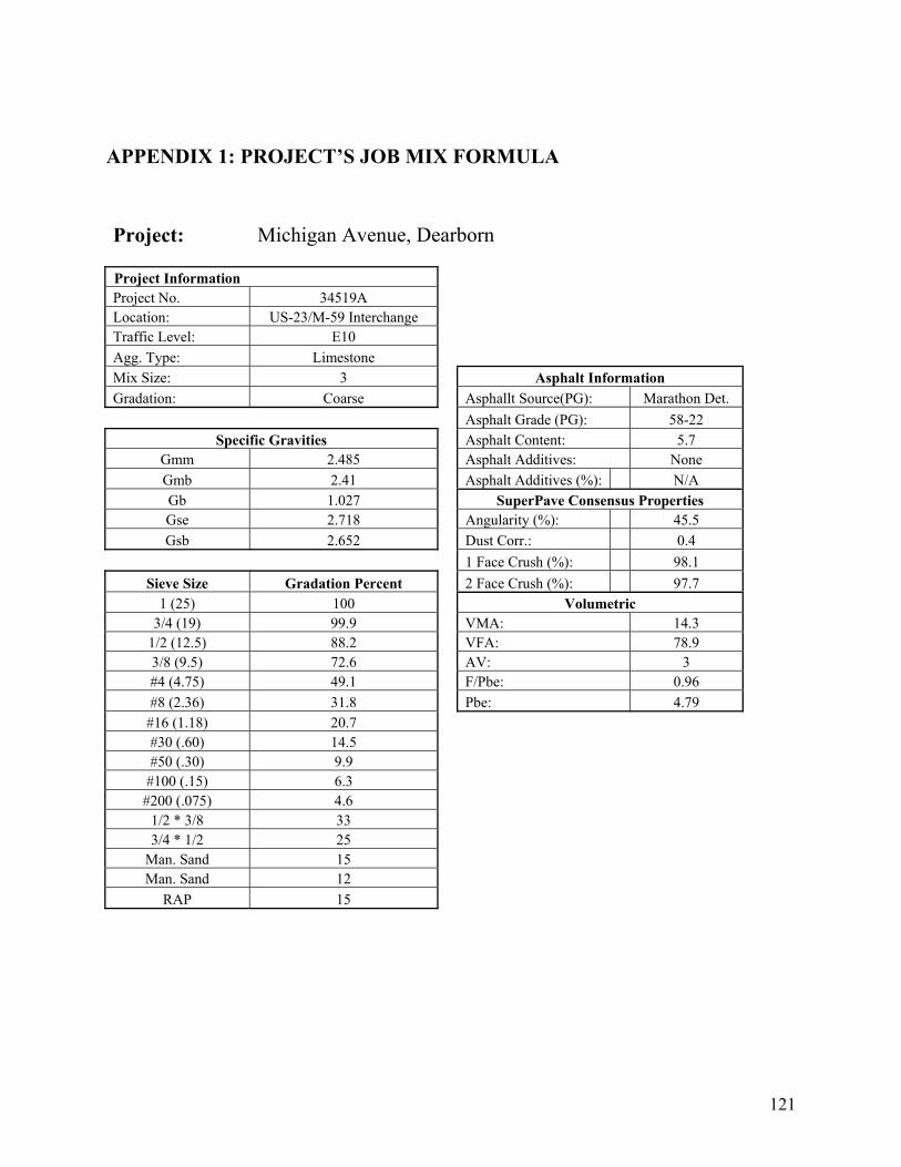
121

APPENDIX 1: PROJECT’S JOB MIX FORMULA

Project: Michigan Avenue, Dearborn Project Information Project No. 34519A Location: US-23/M-59 Interchange Traffic Level: E10 Agg. Type: Limestone Mix Size: 3 Asphalt Information Gradation: Coarse Asphallt Source(PG): Marathon Det. Asphalt Grade (PG): 58-22

Specific Gravities Asphalt Content: 5.7 Gmm 2.485 Asphalt Additives: None Gmb 2.41 Asphalt Additives (%): N/A Gb 1.027 SuperPave Consensus Properties Gse 2.718 Angularity (%): 45.5 Gsb 2.652 Dust Corr.: 0.4

1 Face Crush (%): 98.1 Sieve Size Gradation Percent 2 Face Crush (%): 97.7

1 (25) 100 Volumetric 3/4 (19) 99.9 VMA: 14.3

1/2 (12.5) 88.2 VFA: 78.9 3/8 (9.5) 72.6 AV: 3 #4 (4.75) 49.1 F/Pbe: 0.96 #8 (2.36) 31.8 Pbe: 4.79

#16 (1.18) 20.7 #30 (.60) 14.5 #50 (.30) 9.9

#100 (.15) 6.3 #200 (.075) 4.6

1/2 * 3/8 33 3/4 * 1/2 25

Man. Sand 15 Man. Sand 12

RAP 15

122

Project: US-23/ M- 59 Brighton

Project Information

Project No. 47064 A Location: Michigan Ave. Traffic Level: E10 Agg. Type: N/A Mix Size: 3 Asphalt Information Gradation: Coarse Asphallt Source(PG): Marathon Det. Asphalt Grade (PG): 58-22 Specific Gravities Asphalt Content: 5.6

Gmm 2.496 Asphalt Additives: None Gmb 2.419 Asphalt Additives (%): N/A Gb 1.025 SuperPave Consensus Properties Gse 2.725 Angularity (%): 45.4 Gsb 2.634 Dust Corr.: 0


1 (25) 100 Volumetric 3/4 (19) 100 VMA: 13.3

1/2 (12.5) 85.3 VFA: 76.7 3/8 (9.5) 71 AV: 3.1 #4 (4.75) 43.8 F/Pbe: 1.2 #8 (2.36) 25.9 Pbe: 4.42

#16 (1.18) 17.5 #30 (.60) 13.3 #50 (.30) 9.6

#100 (.15) 6.8 #200 (.075) 5.3

#4's 33 1/2" 25

Man. Sand 15 Man. Sand Sora 12

RAP 15

123

Project: Vandyke, Detroit

Project Information Project No. 46273A

Location: M 53/28 Mi to 31 Mi

Rd. Traffic Level: E30 Agg. Type: N/A Mix Size: 3 Asphalt Information Gradation: Coarse Asphallt Source(PG): Marathon Det. Asphalt Grade (PG): 64-22

Specific Gravities Asphalt Content: 5.2 Gmm 5.577 Asphalt Additives: None

Gmb 2.495 Asphalt Additives (%): N/A

Gb 1.031 SuperPave Consensus Properties Gse 2.81 Angularity (%): 45.5 Gsb 2.769 Dust Corr.: 0.4


1 (25) 100 Volumetric 3/4 (19) 98.9 VMA: 14.6

1/2 (12.5) 90 VFA: 78.2 3/8 (9.5) 83.9 AV: 3.2 #4 (4.75) 66.6 F/Pbe: 0.86 #8 (2.36) 43.7 Pbe: 5

#16 (1.18) 30.5 #30 (.60) 21.2 #50 (.30) 11

#100 (.15) 6.2 #200 (.075) 4.3

2NS 15 HL3 8 Otr 43

Mfg. Sand 15 6A 19

RAP N/A

124

Project: M - 26 Trimountain

Project Information Project No. 53244A Location: Hancock Traffic Level: E1 Agg. Type: N/A Mix Size: 4 Asphalt Information Gradation: N/A Asphallt Source(PG): Murphy Oil Asphalt Grade (PG): 52-34

Specific Gravities Asphalt Content: 4.4 Gmm 2.496 Asphalt Additives: None Gmb 2.396 Asphalt Additives (%): N/A Gb 1.025 SuperPave Consensus Properties Gse 2.718 Angularity (%): 43.6 Gsb 2.674 Dust Corr.: 0.4

1 Face Crush (%): 90.5 Sieve Size Gradation Percent 2 Face Crush (%): N/A

1 (25) 100 Volumetric 3/4 (19) 100 VMA: 15.2

1/2 (12.5) 93.9 VFA: 73.7 3/8 (9.5) 85 AV: 4 #4 (4.75) 64.8 F/Pbe: 1 #8 (2.36) 51 Pbe: N/A

#16 (1.18) 36.2 #30 (.60) 26.7 #50 (.30) 15.4

#100 (.15) 6.9 #200 (.075) 4.7

Crushed 1 Face 90.5

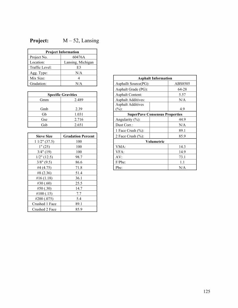
125

Project: M – 52, Lansing

Project Information Project No. 60476A Location: Lansing, Michigan Traffic Level: E3 Agg. Type: N/A Mix Size: 4 Asphalt Information Gradation: N/A Asphallt Source(PG): ABS8505 Asphalt Grade (PG): 64-28

Specific Gravities Asphalt Content: 5.57 Gmm 2.489 Asphalt Additives: N/A

Gmb 2.39 Asphalt Additives (%): 4.9

Gb 1.031 SuperPave Consensus Properties Gse 2.716 Angularity (%): 44.9 Gsb 2.651 Dust Corr.: N/A


1 1/2" (37.5) 100 Volumetric 1" (25) 100 VMA: 14.3

3/4" (19) 100 VFA: 14.9 1/2" (12.5) 98.7 AV: 73.1 3/8" (9.5) 86.6 F/Pbe: 1.1 #4 (4.75) 71.8 Pbe: N/A #8 (2.36) 51.4

#16 (1.18) 36.1 #30 (.60) 25.5 #50 (.30) 14.7

#100 (.15) 7.7 #200 (.075) 5.4

Crushed 1 Face 89.1 Crushed 2 Face 85.9

126

Project: M - 90, Lexington

Project Information Project No. 45440A Location: Port Huron Traffic Level: E3 Agg. Type: N/A Mix Size: 4 Asphalt Information Gradation: N/A Asphallt Source(PG): Marathon Det. Asphalt Grade (PG): 64-28

Specific Gravities Asphalt Content: N/A Gmm 2.474 Asphalt Additives: None


Gb N/A SuperPave Consensus Properties Gse 2.719 Angularity (%): 48.1 Gsb 2.658 Dust Corr.: 0.5


1 1/2" (37.5) 100 Volumetric 1" (25) 100 VMA: 16

3/4" (19) 100 VFA: 75 1/2" (12.5) 99.1 AV: 4 3/8" (9.5) 89.6 F/Pbe: 1.1 #4 (4.75) 74.9 Pbe: N/A #8 (2.36) 56.2

#16 (1.18) 38.6 #30 (.60) 26.8 #50 (.30) 16.5

#100 (.15) 8.7 #200 (.075) 5.6

Crushed 1 Face 96.5 Crushed 2 Face N/A

Asphalt 6 3/8 * 0 18

5/8 * 3/8 18 MFG Sand 64

127

Project: M - 53 Detroit, 8 Mile Road, Detroit

Project Information Project No. 52804A/52805A

Location: M-53/M-3 to M-

102 Traffic Level: E10 Agg. Type: N/A Mix Size: 4 Asphalt Information Gradation: Coarse Asphallt Source(PG): Marathon Det. Asphalt Grade (PG): 70-22




1 Face Crush (%): 95.6

Sieve Size Gradation

Percent 2 Face Crush (%): 92.8 1 (25) 100 Volumetric

3/4 (19) 100 VMA: 15.5 1/2 (12.5) 98.6 VFA: 74.2 3/8 (9.5) 86.7 AV: 4 #4 (4.75) 51.1 F/Pbe: 0.99 #8 (2.36) 29.3 Pbe: 4.55

#16 (1.18) 19.7 #30 (.60) 14 #50 (.30) 9.5

#100 (.15) 6.1 #200 (.075) 4.5

1/2" 33 4 * 3/8" 25 Otr Sand 15

HL3 12 RAP 4

128

Project: 8 mile Road, Detroit Michigan

Project Information Project No. 45164A Location: Utica(Detroit) Traffic Level: E30 Agg. Type: N/A Mix Size: 4 Gradation: N/A

Specific Gravities Gmm 2.554 Gmb 2.439 Gb N/A Gse 2.785 Asphalt Information Gsb 2.728 Asphallt Source(PG): Marathon Det.

Asphalt Grade (PG): 70-22


Percent Asphalt Content: 5.3 1 1/2" (37.5) 100 Asphalt Additives: None

1" (25) 100 Asphalt Additives (%): N/A 3/4" (19) 100 SuperPave Consensus Properties

1/2" (12.5) 99 Angularity (%): 47.1 3/8" (9.5) 87.3 Dust Corr.: 0 #4 (4.75) 55.7 1 Face Crush (%): 96.7 #8 (2.36) 29 2 Face Crush (%): 94

#16 (1.18) 18.8 Volumetric #30 (.60) 14 VMA: 15.3 #50 (.30) 10 VFA: 70.6

#100 (.15) 6.6 AV: 4.5 #200 (.075) 4.8 F/Pbe: 1

Crushed 1 Face 96.7 Pbe: N/A Crushed 2 Face 94

Asphalt 5.3 3/8 CLEAR 17 1/2" x 3/8" 21 Otr Sand 23

Mfg. Sand 21 1/2 " 18

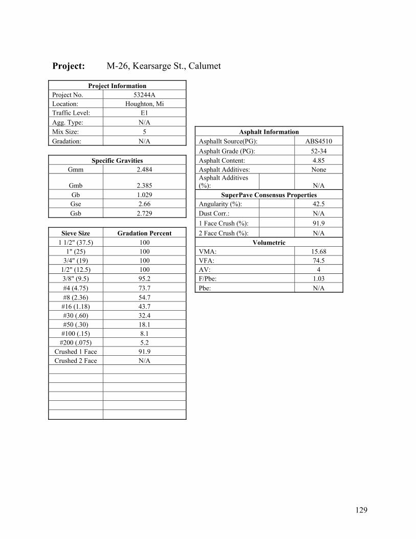
129

Project: M-26, Kearsarge St., Calumet

Project Information Project No. 53244A Location: Houghton, Mi Traffic Level: E1 Agg. Type: N/A Mix Size: 5 Asphalt Information Gradation: N/A Asphallt Source(PG): ABS4510 Asphalt Grade (PG): 52-34





1 1/2" (37.5) 100 Volumetric 1" (25) 100 VMA: 15.68

3/4" (19) 100 VFA: 74.5 1/2" (12.5) 100 AV: 4 3/8" (9.5) 95.2 F/Pbe: 1.03 #4 (4.75) 73.7 Pbe: N/A #8 (2.36) 54.7

#16 (1.18) 43.7 #30 (.60) 32.4 #50 (.30) 18.1

#100 (.15) 8.1 #200 (.075) 5.2


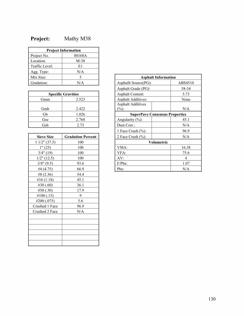
130

Project: Mathy M38

Project Information Project No. 80168A Location: M-38 Traffic Level: E1 Agg. Type: N/A Mix Size: 5 Asphalt Information Gradation: N/A Asphallt Source(PG): ABS4510 Asphalt Grade (PG): 58-34





1 1/2" (37.5) 100 Volumetric 1" (25) 100 VMA: 16.38

3/4" (19) 100 VFA: 75.6 1/2" (12.5) 100 AV: 4 3/8" (9.5) 93.6 F/Pbe: 1.07 #4 (4.75) 66.9 Pbe: N/A #8 (2.36) 54.4

#16 (1.18) 45.1 #30 (.60) 36.1 #50 (.30) 17.9

#100 (.15) 9 #200 (.075) 5.6


131

Project: US 2 Bessemer, MI Project Information Project No. 488344A Location: Bessemer, MI Traffic Level: E3 Agg. Type: N/A Mix Size: 5 Asphalt Information Gradation: N/A Asphallt Source(PG): Murphy Oil Asphalt Grade (PG): 58-34



Gb 1.027 SuperPave Consensus Properties Gse 2.769 Angularity (%): 43.9 Gsb 2.703 Dust Corr.: 0


1 (25) 100 Volumetric 3/4 (19) 100 VMA: 15.9

1/2 (12.5) 100 VFA: 74.8 3/8 (9.5) 95.2 AV: 4 #4 (4.75) 72 F/Pbe: 1.08 #8 (2.36) 57.2 Pbe: N/A

#16 (1.18) 40.9 #30 (.60) 25.4 #50 (.30) 11.8

#100 (.15) 7 #200 (.075) 4.4

#4's 86.8 1/2 x1/4" 25 Nat. Sand 39

3/8 Dense Washed 19 Man. Sand 22

132

Project: Auburn Hill

Project Information

Project No. 84049A Location: Auburn Hills, Mi Traffic Level: E10 Agg. Type: N/A Mix Size: 5 Asphalt Information Gradation: N/A Asphallt Source(PG): Marathon Det. Asphalt Grade (PG): 64-22 Specific Gravities Asphalt Content: 5.66

Gmm 2.473 Asphalt Additives: None


Gb 1.032 SuperPave Consensus Properties Gse 2.739 Angularity (%): 45.8 Gsb 2.637 Dust Corr.: 0


1 (25) 100 Volumetric 3/4 (19) 100 VMA: 15.83

1/2 (12.5) 99.5 VFA: 74.73 3/8 (9.5) 97.4 AV: 4 #4 (4.75) 67.4 F/Pbe: 1.25 #8 (2.36) 37.5 Pbe: N/A #16 (1.18) 23.5 #30 (.60) 17.1 #50 (.30) 12 #100 (.15) 7.9

#200 (.075) 8.4 Crushed 1 Face 97.3 Crushed 2 Face 96.7

Man. Sand 30 Man. Sand #6 19

3/8x#4 25 31A 10

133

Project: Brighton

Project Information

Project No. 83707A Location: Brighton, Mi Traffic Level: E10 Agg. Type: N/A Mix Size: 5 Asphalt Information Gradation: N/A Asphallt Source(PG): Marathon Det. Asphalt Grade (PG): 64-22 Specific Gravities Asphalt Content: 6.31



Gb 1.032 SuperPave Consensus Properties Gse 2.749 Angularity (%): 45.2 Gsb 2.619 Dust Corr.: 0.4

1 Face Crush (%): 98.2



3/4 (19) 100 VMA: 15.68 1/2 (12.5) 99.7 VFA: 74.43 3/8 (9.5) 98.2 AV: 4 #4 (4.75) 88.2 F/Pbe: 1.2 #8 (2.36) 48.8 Pbe: N/A

#16 (1.18) 26.5 #30 (.60) 17.4 #50 (.30) 11.8

#100 (.15) 7.6 #200 (.075) 6.2

Crushed 1 Face 98.2 Crushed 2 Face 98.1

RockWood Man. Sand 18

Sora Man. Sand 33 Sora 3/8x#4 29

3/8 4 Blasst Fumed 10

134

Project: I - 75 Clarkston, Flint Project Information Project No. 45446A Location: Clarkston, MI Traffic Level: E30 Agg. Type: N/A Mix Size: 5 Asphalt Information Gradation: N/A Asphallt Source(PG): t and M Oil Asphalt Grade (PG): 70-22

Specific Gravities Asphalt Content: 6 Gmm 2.564 Asphalt Additives: None Gmb 2.463 Asphalt Additives (%): N/A Gb N/A SuperPave Consensus Properties Gse 2.828 Angularity (%): 48.2 Gsb 2.746 Dust Corr.: 0

1 Face Crush (%): 25 Sieve Size Gradation Percent 2 Face Crush (%): 15

1 (25) 100 Volumetric 3/4 (19) 100 VMA: 15.7

1/2 (12.5) 100 VFA: 74.7 3/8 (9.5) 97.5 AV: 4 #4 (4.75) 70.6 F/Pbe: N/A #8 (2.36) 42.6 Pbe: N/A

#16 (1.18) 27.3 #30 (.60) 18.1 #50 (.30) 12.7

#100 (.15) 8.2 #200 (.075) 5.3

Crushed 1 Face 25 Crushed 2 Face 15

Man. Sand 20 HL1 10 3/8x4 10

Fish Lake 10 Lime Sand 15 Trap Sand 35

135

Project: I-75 Toledo

Project Information

Project No. 74577A Location: Jan-75 Traffic Level: E30 Agg. Type: N/A Mix Size: 5 Asphalt Information Gradation: Coarse Asphallt Source(PG): 6505 MPM Oil Asphalt Grade (PG): 70-22 Specific Gravities Asphalt Content: 5.4



Gb 1.029 SuperPave Consensus Properties Gse 2.737 Angularity (%): 46 Gsb 2.711 Dust Corr.: 0.4

1 Face Crush (%): 98



3/4 (19) 100 VMA: 15.9 1/2 (12.5) 100 VFA: 74.9 3/8 (9.5) 95.4 AV: 4 #4 (4.75) 64.5 F/Pbe: 1.07 #8 (2.36) 36.4 Pbe: 5.05

#16 (1.18) 22.4 #30 (.60) 16.5 #50 (.30) 11.6

#100 (.15) 7.4 #200 (.075) 5.4

3/8x4 10 Man Sand 28 Fine Crush 10 Man. Sand 32 1/4 Chip 10 1/2 Clear 10

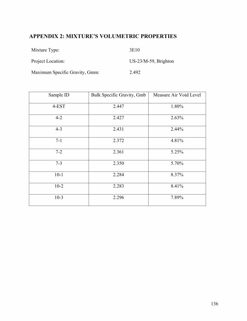
136

APPENDIX 2: MIXTURE’S VOLUMETRIC PROPERTIES

Mixture Type: 3E10

Project Location: US-23/M-59, Brighton

Maximum Specific Gravity, Gmm: 2.492

Sample ID Bulk Specific Gravity, Gmb Measure Air Void Level

4-EST 2.447 1.80%

4-2 2.427 2.63%

4-3 2.431 2.44%

7-1 2.372 4.81%

7-2 2.361 5.25%

7-3 2.350 5.70%

10-1 2.284 8.37%

10-2 2.283 8.41%

10-3 2.296 7.89%

137

Mixture Type: 3E10

Project Location: Michigan Avenue, Dearborn



4-4 2.437 2.47%

4-7 2.419 3.19%

4-9 2.416 3.31%

7-2 2.338 6.43%

7-4 2.334 6.61%

7-8 2.342 6.26%

10-1 2.266 9.34%

10-7 2.265 9.37%

10-9 2.241 10.31%

138

Mixture Type: 3E30

Project Location: Vandyke, Detroit



4-1 2.489 4.50%

4-2 2.485 4.65%

4-3 2.478 4.94%

7-1 2.409 7.57%

7-2 2.394 8.16%

7-3 2.408 7.59%

139

Mixture Type: 4E1

Project Location: M-26 Trimountain



4-1 2.423 2.85%

4-2 2.424 2.78%

4-3 2.428 2.63%

7-1 2.371 4.91%

7-2 2.359 5.40%

7-3 2.362 5.29%

10-1 2.285 8.38%

10-2 2.286 8.34%

10-3 2.304 7.59%

140

Mixture Type: 4E3

Project Location: M-52, Lansing



4-A 2.395 3.91%

4-B 2.394 3.95%

4-C 2.395 3.91%

7-A 2.329 6.56%

7-B 2.325 6.74%

7-C 2.295 7.94%

10-A 2.255 9.54%

10-B 2.255 9.53%

10-C 2.254 9.57%

141

Mixture Type: 4E3

Project Location: M-90, Lexington



4-2 2.417 0.61%

4-6 2.393 1.57%

4-8 2.381 2.07%

7-3 2.353 3.24%

7-4 2.348 3.44%

7-9 2.329 4.22%

10-1 2.247 7.59%

10-5 2.251 7.41%

10-8 2.240 7.87%

142

Mixture Type: 4E10

Project Location: M-53/M-3 to M-102, Detroit



4-1 2.485 3.54%

4-2 2.494 3.19%

4-3 2.488 3.42%

4-4 2.474 3.98%

4-5 2.470 4.14%

4-6 2.493 3.22%

4-7 2.470 4.12%

4-8 2.492 3.28%

4-9 2.497 3.09%

7-2 2.430 5.67%

7-3 2.434 5.54%

7-4 2.445 5.11%

10-4 2.327 9.70%

10-3 2.361 8.35%

10-2 2.359 8.45%

143

Mixture Type: 4E30

Project Location: 8 Mile Road, Detroit



4-1 2.468 4.00%

4-2 2.474 3.77%

4-3 2.491 3.11%

7-1 2.409 6.28%

7-3 2.406 6.40%

7-4 2.404 6.49%

10-1 2.266 11.82%

10-2 2.268 11.77%

10-3 2.261 12.04%

144

Mixture Type: 5E1

Project Location: M-26, Kearsarge St., Calumet



4-2 2.370 4.71%

4-3 2.381 4.26%

4-4 2.389 3.93%

7-1 2.338 5.99%

7-3 2.330 6.30%

7-4 2.331 6.27%

10-2 2.247 9.64%

10-3 2.246 9.69%

10-4 2.256 9.27%

145

Mixture Type: 5E1

Project Location: M-38, Mathy



4-2 2.446 3.23%

4-4 2.424 4.10%

4-8 2.430 3.82%

7-1 2.367 6.32%

7-5 2.375 6.01%

7-7 2.371 6.19%

10-2 2.301 8.94%

10-4 2.302 8.93%

10-6 2.253 10.84%

146

Mixture Type: 5E3

Project Location: US-2 Bessemer



4-1 2.415 5.89%

4-2 2.409 6.11%

4-3 2.418 5.76%

7-3 2.353 8.29%

7-4 2.360 8.02%

7-7 2.354 8.23%

10-2 2.284 10.96%

10-6 2.284 10.99%

10-7 2.262 11.82%

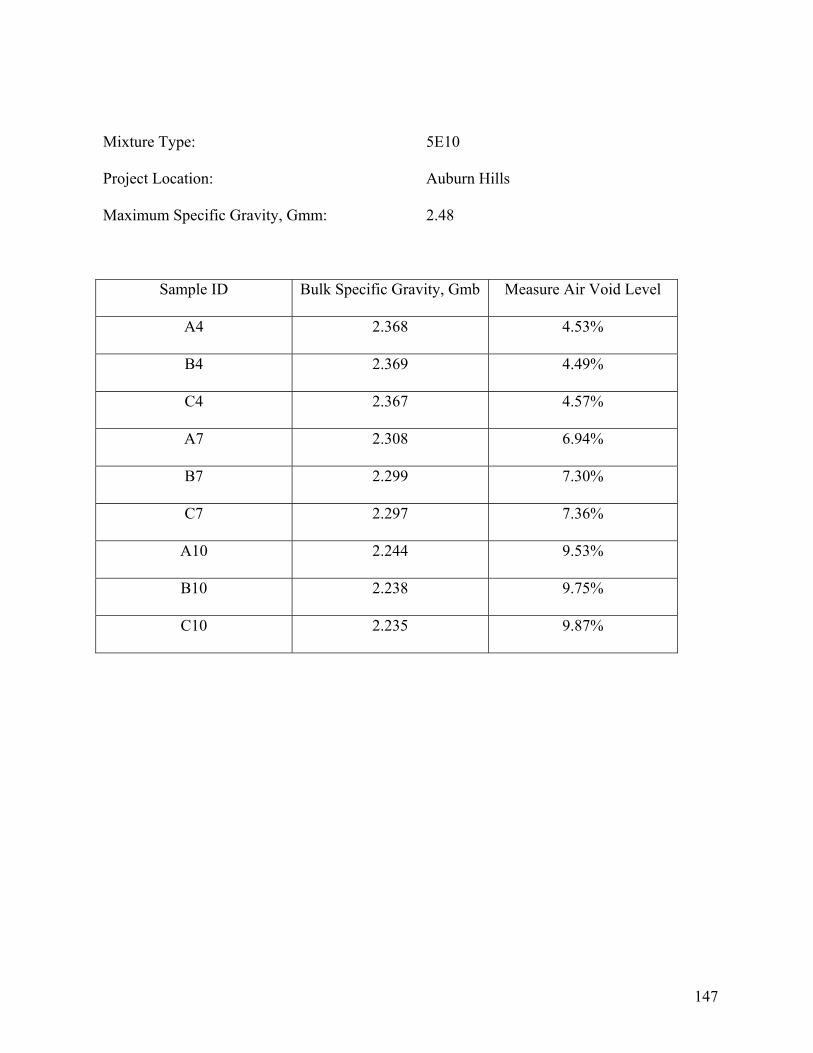
147

Mixture Type: 5E10

Project Location: Auburn Hills



A4 2.368 4.53%

B4 2.369 4.49%

C4 2.367 4.57%

A7 2.308 6.94%

B7 2.299 7.30%

C7 2.297 7.36%

A10 2.244 9.53%

B10 2.238 9.75%

C10 2.235 9.87%

148

Mixture Type: 5E10

Project Location: Brighton



A4 2.365 4.24%

B4 2.376 3.80%

C4 2.365 4.22%

A7 2.293 7.15%

B7 2.300 6.88%

C7 2.294 7.10%

A10 2.130 13.75%

B10 2.231 9.68%

C10 2.248 8.96%

149

Mixture Type: 5E30

Project Location: I-75, Clarkston/Flint



4-1 2.454 4.93%

4-2 2.458 4.76%

4-6 2.451 5.01%

7-2 2.365 8.37%

7-7 2.379 7.82%

7-8 2.367 8.28%

10-1 2.313 10.38%

10-4 2.303 10.76%

10-7 2.294 11.12%

150

Mixture Type: 5E30

Project Location: I-75 Toledo



4-2 2.408 3.92%

4-3 2.402 4.15%

4-4 2.401 4.19%

7-1 2.321 7.37%

7-2 2.333 6.89%

7-6 2.309 7.86%

10-1 2.269 9.45%

10-3 2.265 9.63%

10-6 2.242 10.55%

151

APPENDIX 3: DYNAMIC MODULUS TEST RESULTS

0

5000

10000

15000

20000

25000

30000

0.1 1 10 100

-5C

4C

13C

21.3C

39.2C

Figure 60 Dynamic Modulus for 3E10 I (Project Location: M-59 Brighton) at 4% Air Void

Level

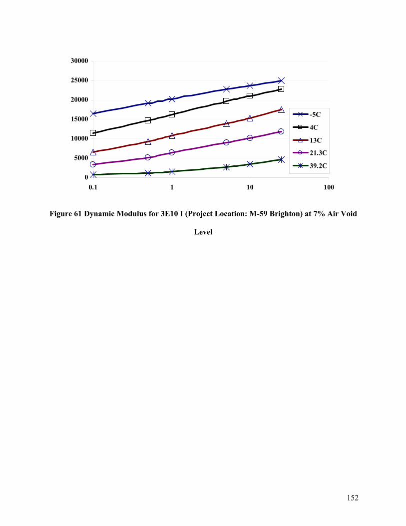
152

0

5000

10000

15000

20000

25000

30000

0.1 1 10 100

-5C

4C

13C

21.3C

39.2C

Figure 61 Dynamic Modulus for 3E10 I (Project Location: M-59 Brighton) at 7% Air Void

Level

153

0

5000

10000

15000

20000

25000

30000

0.1 1 10 100

-5C

4C

13C

21.3C

39.2C


4% Air Void Level

154

0

5000

10000

15000

20000

25000

30000

0.1 1 10 100

-5C

4C

13C

21.3C

39.2C


7% Air Void Level

155

0

5000

10000

15000

20000

25000

30000

0.1 1 10 100

-5C

4C

13C

21.3C

39.2C


Void Level

156

0

5000

10000

15000

20000

25000

30000

0.1 1 10 100

-5C

4C

13C

21.3C

39.2C


Void Level

157

0

5000

10000

15000

20000

25000

0.1 1 10 100

-5C

4C

13C

21.3C

39.2C


Void Level

158

0

5000

10000

15000

20000

25000

0.1 1 10 100

-5C

4C

13C

21.3C

39.2C


Void Level

159

0

5000

10000

15000

20000

25000

0.1 1 10 100

-5C

4C

13C

21.3C

39.2C


Level

160

0

5000

10000

15000

20000

25000

0.1 1 10 100

-5C

4C

13C

21.3C

39.2C


Level

161

0

5000

10000

15000

20000

25000

30000

0.1 1 10 100

-5C

4C

13C

21.3C

39.2C


Level

162

0

5000

10000

15000

20000

25000

30000

0.1 1 10 100

-5C

4C

13C

21.3C

39.2C


Level

163

0

5000

10000

15000

20000

25000

30000

0.1 1 10 100

-5C

4C

13C

21.3C

39.2C


Level

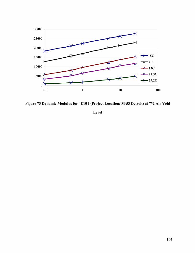
164

0

5000

10000

15000

20000

25000

30000

0.1 1 10 100

-5C

4C

13C

21.3C

39.2C


Level

165

0

5000

10000

15000

20000

25000

30000

35000

0.1 1 10 100

-5C

4C

13C

21.3C

39.2C


Level

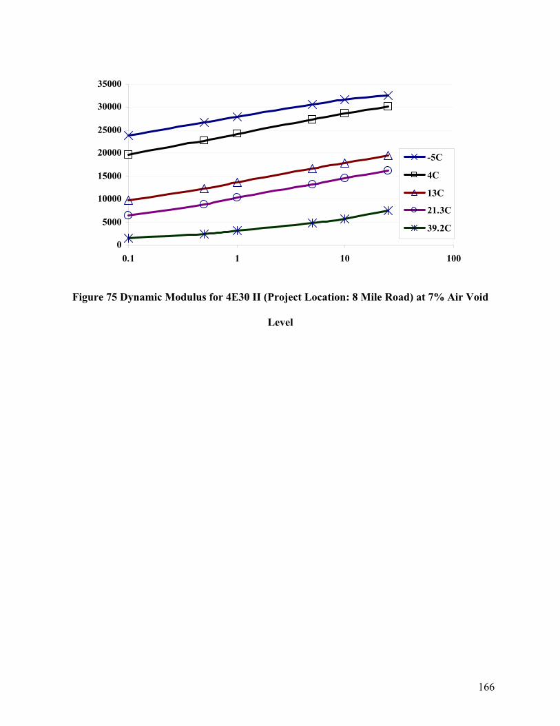
166

0

5000

10000

15000

20000

25000

30000

35000

0.1 1 10 100

-5C

4C

13C

21.3C

39.2C


Level

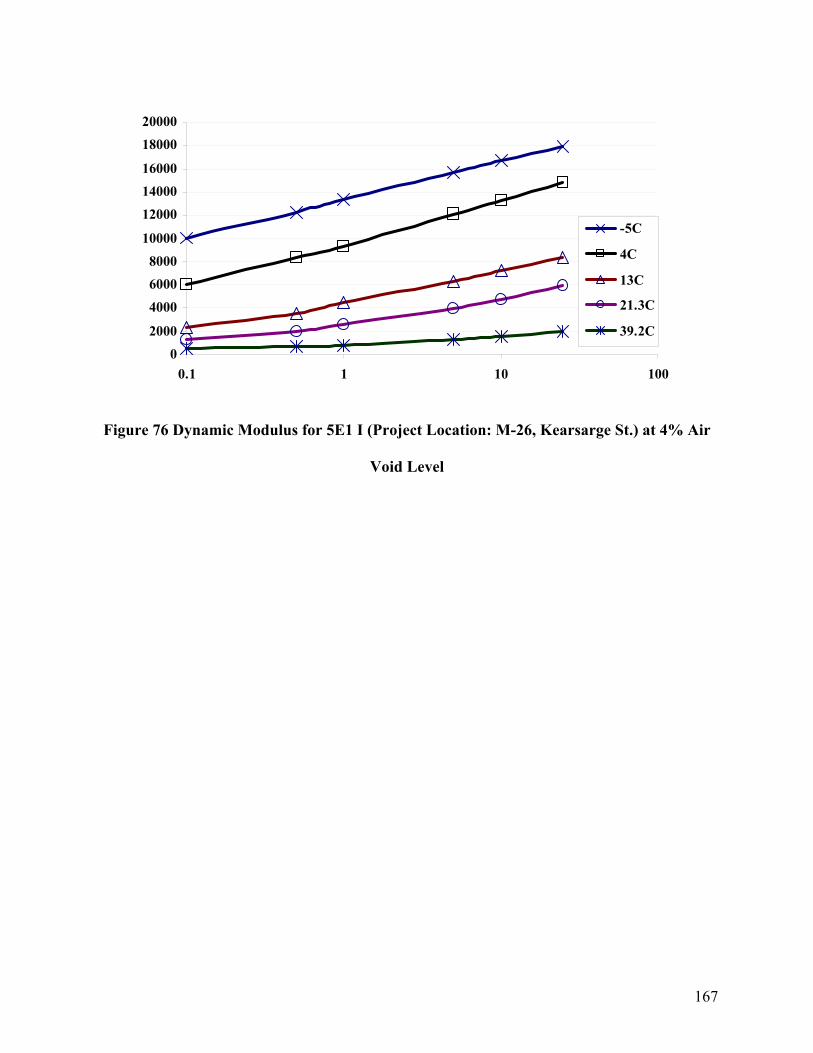
167

0

2000

4000

60008000

10000

12000

1400016000

18000

20000

0.1 1 10 100

-5C

4C

13C

21.3C

39.2C


Void Level

168

0

2000

4000

6000

8000

10000

12000

14000

16000

18000

20000

0.1 1 10 100

-5C

4C

13C

21.3C

39.2C


Void Level

169

0

2000

4000

60008000

10000

12000

1400016000

18000

20000

0.1 1 10 100

-5C

4C

13C

21.3C

39.2C


170

0

5000

10000

15000

20000

25000

30000

0.1 1 10 100

-5C

4C

13C

21.3C

39.2C


171

0

2000

4000

6000

8000

10000

12000

14000

16000

18000

0.1 1 10 100

-5C

4C

13C

21.3C

39.2C


Level

172

0

2000

4000

6000

8000

10000

12000

14000

16000

18000

0.1 1 10 100

-5C

4C

13C

21.3C

39.2C


Level

173

0

5000

10000

15000

20000

25000

30000

0.1 1 10 100

-5C

4C

13C

21.3C

39.2C


Level

174

0

5000

10000

15000

20000

25000

30000

0.1 1 10 100

-5C

4C

13C

21.3C

39.2C


Level

175

0

5000

10000

15000

20000

25000

0.1 1 10 100

-5C

4C

13C

21.3C

39.2C


Level

176

0

5000

10000

15000

20000

25000

0.1 1 10 100

-5C

4C

13C

21.3C

39.2C


Level

177

0

5000

10000

15000

20000

25000

30000

0.1 1 10 100

-5C

4C

13C

21.3C

39.2C

Figure 86 Dynamic Modulus for 5E30 I (Project Location: I-75 Clarkston) at 4% Air Void

Level

178

0

5000

10000

15000

20000

25000

30000

0.1 1 10 100

-5C

4C

13C

21.3C

39.2C

Figure 87 Dynamic Modulus for 5E30 I (Project Location: I-75 Clarkston) at 7% Air Void

Level

179

0

5000

10000

15000

20000

25000

0.1 1 10 100

-5C

4C

13C

21.3C

39.2C


Level

180

0

5000

10000

15000

20000

25000

0.1 1 10 100

-5C

4C

13C

21.3C

39.2C


Level

181

APPENDIX 4: DYNAMIC MODULUS MASTER CURVES

0

5000

10000

15000

20000

25000

-8 -6 -4 -2 0 2


Dyn

amic

Mod

ulus

(MPa

)

Figure 90 Master Curve of Dynamic Modulus for 3E10 I (Project Location: M-59 Brighton)

Mixture with 4% Air Void Level at the Reference Temperature of -5°C

182

0

5000

10000

15000

20000

25000

-8 -6 -4 -2 0 2


Dyn

amic

Mod

ulus

(MPa

)

Figure 91 Master Curve of Dynamic Modulus for 3E10 I (Project Location: M-59 Brighton)


183

0

5000

10000

15000

20000

25000

-8 -6 -4 -2 0 2


Dyn

amic

Mod

ulus

(MPa

)

Figure 92 Master Curve of Dynamic Modulus for 3E10 II (Project Location: Michigan Ave,

Dearborn) Mixture with 4% Air Void Level at the Reference Temperature of -5°C

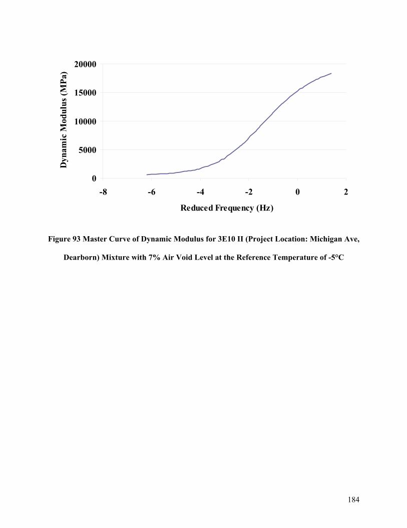
184

0

5000

10000

15000

20000

-8 -6 -4 -2 0 2


Dyn

amic

Mod

ulus

(MPa

)

Figure 93 Master Curve of Dynamic Modulus for 3E10 II (Project Location: Michigan Ave,

Dearborn) Mixture with 7% Air Void Level at the Reference Temperature of -5°C

185

0

5000

10000

15000

20000

25000

30000

-8 -6 -4 -2 0 2


Dyn

amic

Mod

ulus

(MPa

)

Figure 94 Master Curve of Dynamic Modulus for 3E30 I (Project Location: Vandyke, Detroit)


186

0

5000

10000

15000

20000

25000

-8 -6 -4 -2 0 2


Dyn

amic

Mod

ulus

(MPa

)

Figure 95 Master Curve of Dynamic Modulus for 3E30 I (Project Location: Vandyke, Detroit)


187

0

5000

10000

15000

20000

25000

-8 -6 -4 -2 0 2


Dyn

amic

Mod

ulus

(MPa

)

Figure 96 Master Curve of Dynamic Modulus for 4E1 I (Project Location: Tri Mt., Hancock)


188

0

5000

10000

15000

20000

-8 -6 -4 -2 0 2


Dyn

amic

Mod

ulus

(MPa

)

Figure 97 Master Curve of Dynamic Modulus for 4E1 I (Project Location: Tri Mt., Hancock)


189

0

5000

10000

15000

20000

25000

-8 -6 -4 -2 0 2


Dyn

amic

Mod

ulus

(MPa

)

Figure 98 Master Curve of Dynamic Modulus for 4E3 I (Project Location: Lansing, MI) Mixture

with 4% Air Void Level at the Reference Temperature of -5°C

190

0

5000

10000

15000

20000

-8 -6 -4 -2 0 2


Dyn

amic

Mod

ulus

(MPa

)

Figure 99 Master Curve of Dynamic Modulus for 4E3 I (Project Location: Lansing, MI) Mixture


191

0

5000

10000

15000

20000

25000

-8 -6 -4 -2 0 2


Dyn

amic

Mod

ulus

(MPa

)

Figure 100 Master Curve of Dynamic Modulus for 4E3 II (Project Location: Lexington) Mixture


192

0

5000

10000

15000

20000

-8 -6 -4 -2 0 2


Dyn

amic

Mod

ulus

(MPa

)

Figure 101 Master Curve of Dynamic Modulus for 4E3 II (Project Location: Lexington) Mixture


193

0

5000

10000

15000

20000

25000

30000

-8 -6 -4 -2 0 2


Dyn

amic

Mod

ulus

(MPa

)

Figure 102 Master Curve of Dynamic Modulus for 4E10 I (Project Location: M-53 Detroit)


194

0

5000

10000

15000

20000

25000

-8 -6 -4 -2 0 2


Dyn

amic

Mod

ulus

(MPa

)

Figure 103 Master Curve of Dynamic Modulus for 4E10 I (Project Location: M-53 Detroit)


195

0

5000

10000

15000

20000

25000

30000

35000

-8 -6 -4 -2 0 2


Dyn

amic

Mod

ulus

(MPa

)



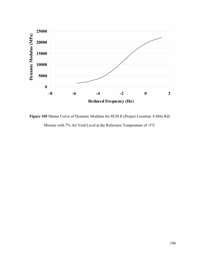
196

0

5000

10000

15000

20000

25000

-8 -6 -4 -2 0 2


Dyn

amic

Mod

ulus

(MPa

)



197

0

5000

10000

15000

20000

-8 -6 -4 -2 0 2


Dyn

amic

Mod

ulus

(MPa

)

Figure 106 Master Curve of Dynamic Modulus for 5E1 I (Project Location: M-26, Kearsarge St.)


198

0

5000

10000

15000

20000

-8 -6 -4 -2 0 2


Dyn

amic

Mod

ulus

(MPa

)

Figure 107 Master Curve of Dynamic Modulus for 5E1 I (Project Location: M-26, Kearsarge St.)


199

0

5000

10000

15000

20000

-8 -6 -4 -2 0 2


Dyn

amic

Mod

ulus

(MPa

)

Figure 108 Master Curve of Dynamic Modulus for 5E1 II (Project Location: M-38) Mixture


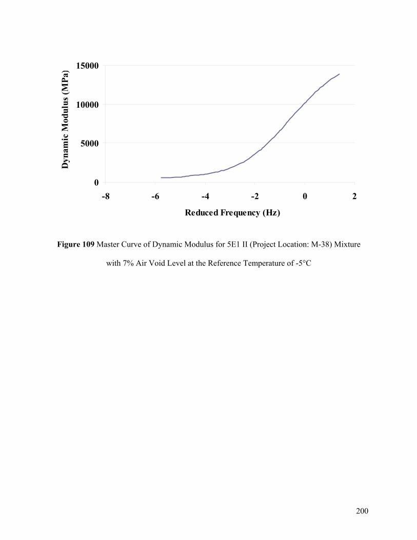
200

0

5000

10000

15000

-8 -6 -4 -2 0 2


Dyn

amic

Mod

ulus

(MPa

)

Figure 109 Master Curve of Dynamic Modulus for 5E1 II (Project Location: M-38) Mixture


201

0

5000

10000

15000

20000

-8 -6 -4 -2 0 2


Dyn

amic

Mod

ulus

(MPa

)

Figure 110 Master Curve of Dynamic Modulus for 5E3 I (Project Location: Bessemer, MI)


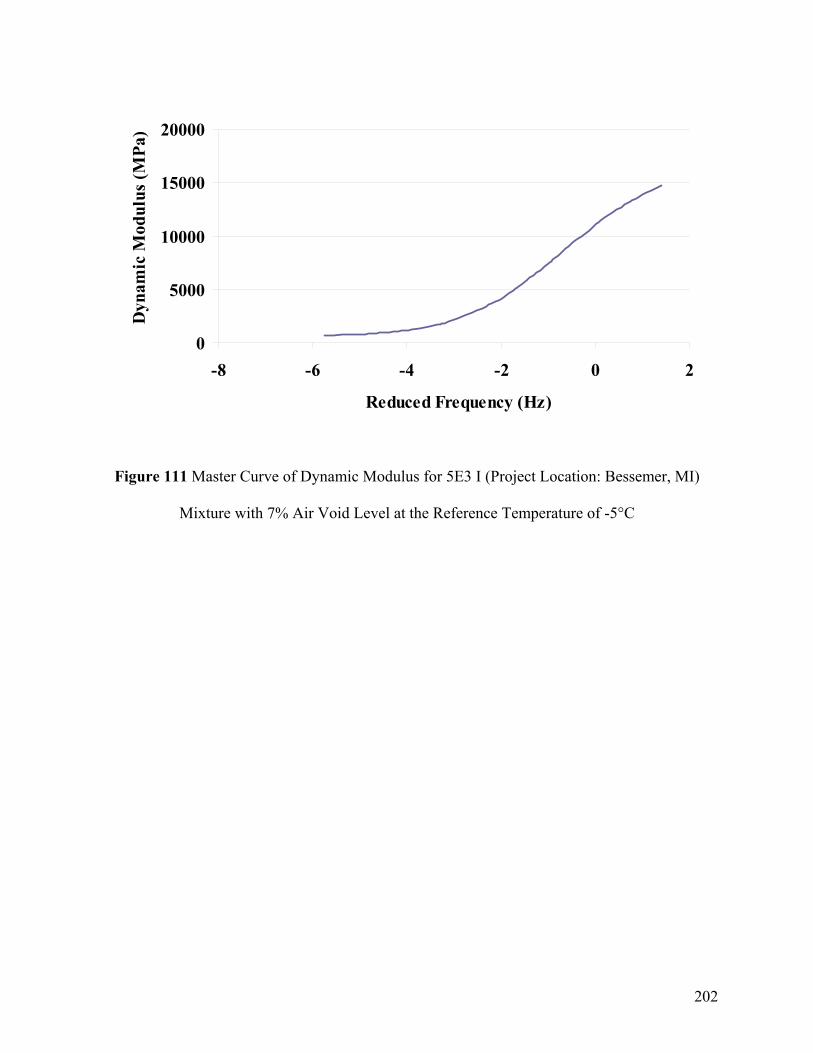
202

0

5000

10000

15000

20000

-8 -6 -4 -2 0 2


Dyn

amic

Mod

ulus

(MPa

)

Figure 111 Master Curve of Dynamic Modulus for 5E3 I (Project Location: Bessemer, MI)


203

0

5000

10000

15000

20000

25000

30000

-8 -6 -4 -2 0 2


Dyn

amic

Mod

ulus

(MPa

)

Figure 112 Master Curve of Dynamic Modulus for 5E10 I (Project Location: Auburn Hills)


204

0

5000

10000

15000

20000

25000

-8 -6 -4 -2 0 2


Dyn

amic

Mod

ulus

(MPa

)

Figure 113 Master Curve of Dynamic Modulus for 5E10 I (Project Location: Auburn Hills)


205

0

5000

10000

15000

20000

25000

-8 -6 -4 -2 0 2


Dyn

amic

Mod

ulus

(MPa

)

Figure 114 Master Curve of Dynamic Modulus for 5E10 II (Project Location: Oregon, OH)


206

0

5000

10000

15000

20000

25000

-8 -6 -4 -2 0 2


Dyn

amic

Mod

ulus

(MPa

)

Figure 115 Master Curve of Dynamic Modulus for 5E10 II (Project Location: Oregon, OH)


207

0

5000

10000

15000

20000

25000

30000

-8 -6 -4 -2 0 2


Dyn

amic

Mod

ulus

(MPa

)

Figure 116 Master Curve of Dynamic Modulus for 5E30 I (Project Location: I-75 Clarkston)


208

0

5000

10000

15000

20000

25000

-8 -6 -4 -2 0 2


Dyn

amic

Mod

ulus

(MPa

)

Figure 117 Master Curve of Dynamic Modulus for 5E30 I (Project Location: I-75 Clarkston)


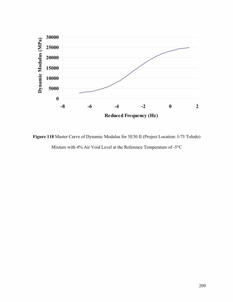
209

0

5000

10000

15000

20000

25000

30000

-8 -6 -4 -2 0 2


Dyn

amic

Mod

ulus

(MPa

)

Figure 118 Master Curve of Dynamic Modulus for 5E30 II (Project Location: I-75 Toledo)


210

0

5000

10000

15000

20000

25000

-8 -6 -4 -2 0 2


Dyn

amic

Mod

ulus

(MPa

)

Figure 119 Master Curve of Dynamic Modulus for 5E30 II (Project Location: I-75 Toledo)


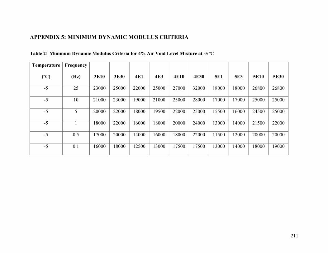
211

APPENDIX 5: MINIMUM DYNAMIC MODULUS CRITERIA


Temperature

(ºC)

Frequency

(Hz) 3E10 3E30 4E1 4E3 4E10 4E30 5E1 5E3 5E10 5E30

-5 25 23000 25000 22000 25000 27000 32000 18000 18000 26800 26800

-5 10 21000 23000 19000 21000 25000 28000 17000 17000 25000 25000

-5 5 20000 22000 18000 19500 22000 25000 15500 16000 24500 25000

-5 1 18000 22000 16000 18000 20000 24000 13000 14000 21500 22000

-5 0.5 17000 20000 14000 16000 18000 22000 11500 12000 20000 20000

-5 0.1 16000 18000 12500 13000 17500 17500 13000 14000 18000 19000

212


Temperature

(ºC)

Frequency

(Hz) 3E10 3E30 4E1 4E3 4E10 4E30 5E1 5E3 5E10 5E30

4 25 18000 20000 12500 17000 20500 23500 12500 12500 23500 23500

4 10 16000 18000 11000 16000 19500 21000 11000 11000 22000 22000

4 5 15000 17000 10000 14500 16000 18000 10000 10000 20000 20000

4 1 13000 15000 8500 12000 14500 16500 7500 7500 17500 17500

4 0.5 11000 13000 7500 11000 13500 18000 6500 6500 15500 15500

4 0.1 10000 12000 6000 8500 12500 15000 4500 4500 12500 13500

213


Temperature

(ºC)

Frequency

(Hz) 3E10 3E30 4E1 4E3 4E10 4E30 5E1 5E3 5E10 5E30

13 25 13000 15000 10000 11500 13500 15500 8500 9000 16500 16500

13 10 11000 13500 9000 10000 12000 14000 7000 7500 14500 14500

13 5 9500 11500 8000 9500 10500 12500 6000 6500 13500 13500

13 1 8000 10000 6000 7500 9000 11500 4000 5000 10500 10500

13 0.5 6500 8000 4500 6500 7500 10000 3500 3500 9000 9500

13 0.1 5000 7000 3000 4000 5000 8000 1900 2500 6500 7500

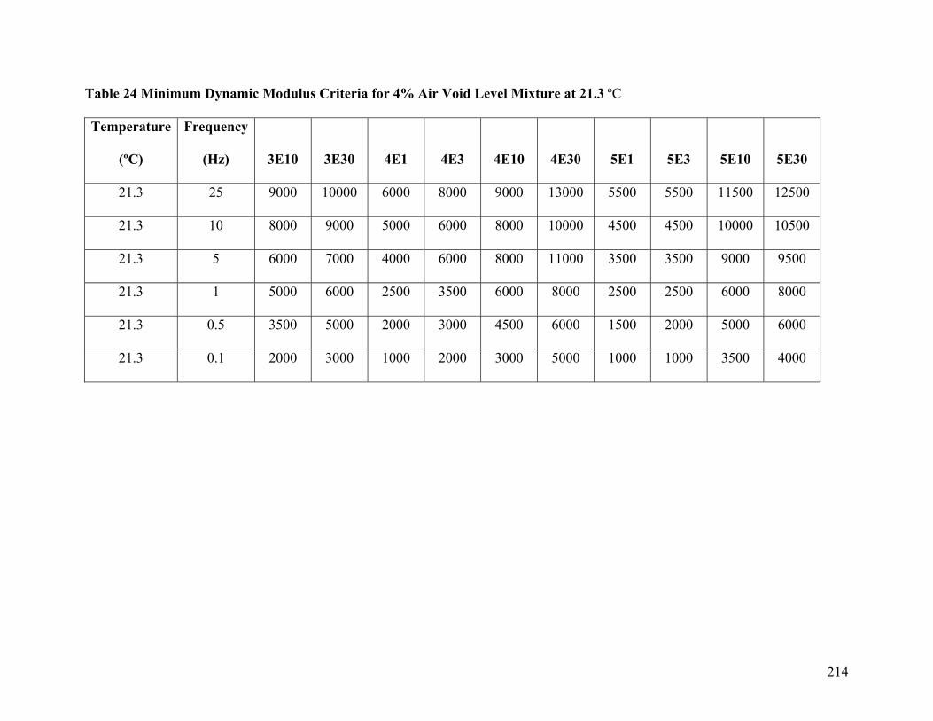
214


Temperature

(ºC)

Frequency

(Hz) 3E10 3E30 4E1 4E3 4E10 4E30 5E1 5E3 5E10 5E30

21.3 25 9000 10000 6000 8000 9000 13000 5500 5500 11500 12500

21.3 10 8000 9000 5000 6000 8000 10000 4500 4500 10000 10500

21.3 5 6000 7000 4000 6000 8000 11000 3500 3500 9000 9500

21.3 1 5000 6000 2500 3500 6000 8000 2500 2500 6000 8000

21.3 0.5 3500 5000 2000 3000 4500 6000 1500 2000 5000 6000

21.3 0.1 2000 3000 1000 2000 3000 5000 1000 1000 3500 4000

215


Temperature

(ºC)

Frequency

(Hz) 3E10 3E30 4E1 4E3 4E10 4E30 5E1 5E3 5E10 5E30

39.2 25 2500 4500 1500 3000 3500 5000 2000 2000 4500 5000

39.2 10 2000 3500 1000 2000 3500 4500 1500 1500 3500 4000

39.2 5 1500 3000 1000 1800 2500 4000 1150 1150 2500 3000

39.2 1 800 1500 700 1000 1500 2000 800 800 1300 2000

39.2 0.5 600 1000 500 700 1000 1500 700 700 800 1500

39.2 0.1 400 600 400 500 700 900 550 550 600 900

216


Temperature

(ºC)

Frequency

(Hz) 3E10 3E30 4E1 4E3 4E10 4E30 5E1 5E3 5E10 5E30

-5 25 19000 21000 17000 20500 21000 22000 17000 17000 22500 22500

-5 10 18000 20000 16000 20000 20500 21000 16000 16000 21500 21500

-5 5 16000 19000 14500 18500 20000 20000 14500 15000 20500 20500

-5 1 13000 16000 12000 16000 17000 18000 12000 12000 18500 18500

-5 0.5 12000 15000 11000 15000 16000 17000 11000 11000 16500 17000

-5 0.1 10000 12000 8500 12000 13000 14000 8500 9000 15000 15000

217


Temperature

(ºC)

Frequency

(Hz) 3E10 3E30 4E1 4E3 4E10 4E30 5E1 5E3 5E10 5E30

4 25 16000 16000 10500 12000 16000 19000 10500 10500 19500 19500

4 10 14000 14500 9500 11000 14000 17000 9500 10000 18500 18500

4 5 12000 12500 8500 10000 13000 16000 8500 9000 17000 17500

4 1 10000 10500 6500 11500 12500 15500 6500 6500 14500 15000

4 0.5 8000 9000 5500 10500 12000 13500 5500 6000 13000 14000

4 0.1 7000 8000 4000 8500 10000 11000 4000 5000 10500 12000

218


Temperature

(ºC)

Frequency

(Hz) 3E10 3E30 4E1 4E3 4E10 4E30 5E1 5E3 5E10 5E30

13 25 10000 12000 6000 8000 12500 13000 7000 7000 14000 14000

13 10 8000 10000 5500 6000 10000 11000 6000 6000 12500 12500

13 5 6500 8500 5000 5500 8500 10000 5000 5000 11000 11000

13 1 5500 6500 4000 6000 7500 8500 4000 4000 9000 9000

13 0.5 4500 6500 3000 5500 6500 7500 3000 3500 7500 8000

13 0.1 3000 4000 2000 4000 4500 6000 1700 2000 5000 6000

219


Temperature

(ºC)

Frequency

(Hz) 3E10 3E30 4E1 4E3 4E10 4E30 5E1 5E3 5E10 5E30

21.3 25 6500 8000 4000 6500 8500 10000 4000 4000 10000 10500

21.3 10 5500 7000 4000 7000 8000 9500 3000 3000 8000 10000

21.3 5 5000 6500 3500 6000 7000 8000 4000 5000 7000 8500

21.3 1 3000 5000 2000 3500 6000 8000 2000 2500 5000 6500

21.3 0.5 5000 5500 2500 3000 4000 5000 1500 2000 4000 5500

21.3 0.1 1500 3000 1000 1500 2500 4000 1000 1000 2500 3500

220


Temperature

(ºC)

Frequency

(Hz) 3E10 3E30 4E1 4E3 4E10 4E30 5E1 5E3 5E10 5E30

39.2 25 2000 3500 1500 3000 4000 4500 1600 1600 4000 4500

39.2 10 1500 3000 1000 2200 3000 4000 1250 1250 3050 3500

39.2 5 1000 2000 700 1000 2000 2500 1000 1000 2400 2850

39.2 1 650 1000 600 750 1300 1550 700 800 1400 1800

39.2 0.5 500 800 400 850 1000 1250 600 600 1000 1300

39.2 0.1 400 600 350 600 750 850 450 450 600 850

rc-1532 - development of specifications for the superpave simple

Documents