RCS-603: COMPUTER GRAPHICSUNIT-IV

Presented By :

Dr. Vinod Jain (Associate Professor, GLBITM)

Unit- IV - Curves and Surfaces:

1. Quadric surfaces

2. Spheres

3. Ellipsoid

4. Blobby objects

5. Introductory concepts of Spline

6. Bspline and Bezier curves and surfaces.

Curves and Surfaces

Curves and Surfaces

• Displays of three dimensional curved lines and surfaces can begenerated from an input set of mathematical functions defining theobjects or from a set of users specified data points.

• When functions are specified, a package can project the definingequations for a curve to the display plane and plot pixel positionsalong the path of the projected function.

Quadric surfaces

• A frequently used class of objects are the quadric surfaces, which aredescribed with second-degree equations (quadratics).

• They include

1. Spheres,

2. Ellipsoids,

3. Paraboloids,

4. Hyperboloids etc.

Quadric surfaces

Sphere

• In Cartesian coordinates, a spherical surface with radius r centered on the coordinate origin is defined as the set of points (x, y, z) that satisfy the equation

Sphere in parametric form

• We can also describe thespherical surface in parametricform, using latitude andlongitude angles.

Sphere in parametric form

Ellipsoid

• An ellipsoidal surface can be described as an extension of a sphericalsurface, where the radii in three mutually perpendicular directionscan have different values.

Ellipsoid

• The Cartesian representation for points over the surface of anellipsoid centered on the origin is

Ellipsoid - Parametric representation

Superquadrics

Superquadrics

• Superquadrics are formed by incorporating additional parametersinto the quadric equations to provide increased flexibility foradjusting object shapes.

• The number of additional parameters used is equal to the dimensionof the object: one parameter for curves and two parameters forsurfaces.

Superquadrics

1. Superellipse

2. Superellipsoid

Superellipse

superellipse

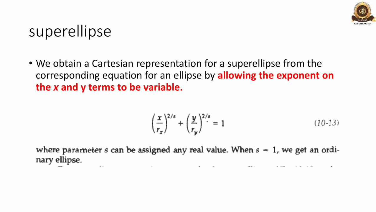
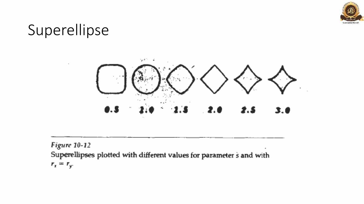
• We obtain a Cartesian representation for a superellipse from the corresponding equation for an ellipse by allowing the exponent on the x and y terms to be variable.

Superellipse – In parametric form

Superellipse

Superellipsoids

Superellipsoids

Superellipsoids

• Figure 10-13 illustrates supersphere shapes that can be generatedusing various values for parameters s, and s2.

• These and other superquadric shapes can be combined to createmore complex structures, such as furniture, threaded bolts, and otherhardware

Superellipsoids

Blobby objects

Blobby objects

Blobby objects

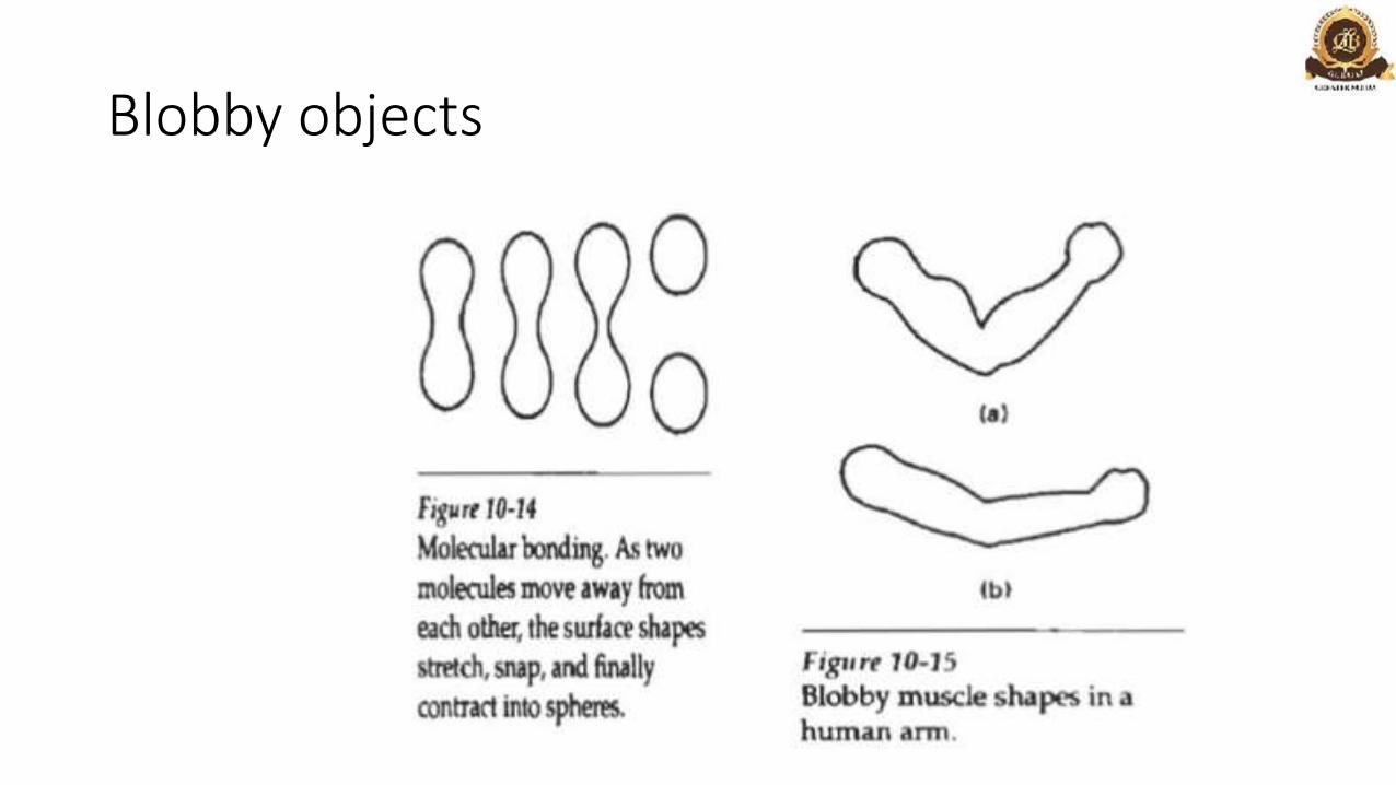
• Some objects do not maintain a fixed shape

• They change their surface characteristics in certain motions

• These objects are referred to as blobby objects, since their shapes show a certain degree of fluidity

• Examples in this class of objects include

1. water droplets

2. melting objects

3. muscle shapes in the human body.

Blobby objects

• Several models have been developed for representing blobby objects as distribution functions over a region of space.

• Combinations of Gaussian density functions, or "bumps“ (Fig 10.16)

Blobby objects

• Several models have been developed for representing blobby objects as distribution functions over a region of space.

• Combinations of Gaussian density functions, or "bumps“ (Fig 10.16)

Blobby objects

• A surface function is then defined as

Blobby objects – Metaballs

Blobby objects

Blobby objects - metaball

• The "metaball" model describes blobby objects as combinations of quadratic density functions of the form

Spline

• Drafting terminology• Spline is a flexible strip that is easily flexed to pass through a series

of design points (control points) to produce a smooth curve.

• Spline curve – a piecewise polynomial (cubic) curve whosefirst and second derivatives are continuous across thevarious curve sections.

Spline Representations

• A spline is a smooth curvedefined mathematicallyusing a set of constraints

• Splines have many uses:• 2D illustration

• Fonts

• 3D Modelling

• Animation

Big Idea

• User specifies control points

• Defines a smooth curve

Control

Points

Control

Points

Curve

Interpolation Vs Approximation

• A spline curve is specified using a set of control points

• There are two ways to fit a curve to these points:• Interpolation - the curve passes

through all of the control points

• Approximation - the curve does not pass through all of the control points

• Approximation for structure or shape

• Interpolation for animation

Convex Hulls• The boundary formed by the set of control points for a spline is

known as a convex hull

• Think of an elastic band stretched around the control points

Control Graphs

• A polyline connecting the control points in order is known as a control graph

• Usually displayed to help designers keep track of their splines

Piecewise cubic splines

Types of Curves

• A curve is an infinitely large set of points. Each point has two neighbors except endpoints. Curves can be broadly classified into three categories −

• explicit, implicit, and parametric curves.

• Implicit Curves

Implicit Curves

• Implicit curve representations define the set of points on a curve by employing a procedure that can test to see if a point in on the curve.

• Usually, an implicit curve is defined by an implicit function of the form −

• f(x, y) = 0

• Eg. A common example is the circle, whose implicit representation is

• x2 + y2 - R2 = 0

Explicit Curves

• A mathematical function y = f(x) can be plotted as a curve.

• Such a function is the explicit representation of the curve.

Parametric curve

• The explicit and implicit curve representations can be used only when the function is known.

• Curves having parametric form are called parametric curves.

• In practice the parametric curves are used.

• Every point on the curve is having two neighbors (other than the end points).

Parametric curve

• A two-dimensional parametric curve has the following form −

• P(t) = f(t), g(t) or P(t) = x(t), y(t)

• The functions f and g become the (x, y) coordinates of any point on the curve, and the points are obtained when the parameter t (or u) is varied over a certain interval [a, b], normally [0, 1].

Parametric Continuity Conditions

• To ensure a smooth transition from one section of a piecewise parametric curve to the next, we can impose various continuity conditions at the connection points.

• If each section of a spline is described with a set of parametric coordinate functions of the form

Parametric Continuity Conditions

• Three types of continuity

1. Zero Order Continuity

2. First Order Continuity

3. Second Order Continuity

Zero Order Continuity

• Two piece of curve must meet at transition point

• Segments have to match ‘nicely’.

• Given two segments P(u) and Q(v).

• We consider the transition of P(1) to Q(0).

• Zero-order parametric continuity

• C0: P(1) = Q(0).

• Endpoint of P(u) coincides with start point Q(v).

First Order Continuity

• First parametric derivatives (tangent lines) of the coordinate functions two successive curve sections are equal at their joining point.

• Segments have to match ‘nicely’.

• Given two segments P(u) and Q(v).

• We consider the transition of P(1) to Q(0).

• First order parametric continuity

• C1: dP(1)/du = dQ(0)/dv.

• Direction of P(1) coincides with direction of Q(0).

Second Order Continuity

• Second-order parametric continuity, or C2 continuity, means that both the first and second parametric derivatives of the two curve sections are the same at the intersection.

• Given two segments P(u) and Q(v).

• We consider the transition of P(1) to Q(0).

• Second order parametric continuity

• C2: d2P(1)/du2 = d2Q(0)/dv2.

• Curvatures in P(1) and Q(0) are equal.

Geometric Continuity

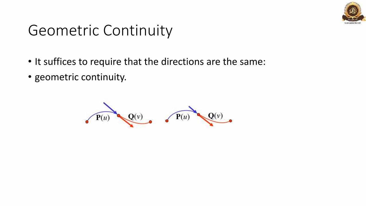
• It suffices to require that the directions are the same:

• geometric continuity.

Geometric Continuity

An alternate method for joining two successive curve sections

Geometric Continuity

An alternate method for joining two successive curve sections

1. Zero Order Geometric Continuity

2. First Order Geometric Continuity

3. Second Order Geometric Continuity

Geometric Continuity

1. Zero Order Geometric Continuity• the two curves sections must have the same coordinate position at the

boundary point ( Same as zero order parametric continuity)

2. First Order Geometric Continuity• the parametric first derivatives are proportional at the intersection of two

successive sections (In parametric continuity these are equal)

3. Second Order Geometric Continuity• both the first and second order derivatives of the two 2.curve sections are

proportional at their boundary

Spline Representation

• There are three equivalent methods for specifying a particular spline representation:

• (1) We can state the set of boundary conditions that are imposed on the spline;

• (2) we can state the matrix that characterizes the spline;

• (3) we can state the set of blending functions

boundary conditions

• Boundary conditions for this curve might be set,

• for example, on the endpoint coordinates x(0) and x(l) and on the parametric first derivatives at the endpoints x'(0) and x ' ( 1 ) .

• Boundary conditions are sufficient to determine the values of the four coefficients ax, bx, cx, and dx.

boundary conditions

Matrix Form• we can obtain the matrix that characterizes this spline curve by first

rewriting Eq as the matrix product

blending functions

Bezier curves

• Bezier curve is discovered by the French engineer Pierre Bézier.

• These curves can be generated under the control of other points. Approximate tangents by using control points are used to generate curve.

Bezier curves

Bezier curves

• The simplest Bézier curve is the straight line from the point P0 to P1.

• A quadratic Bezier curve is determined by three control points.

• A cubic Bezier curve is determined by four control points.

Properties of Bezier curves

• They generally follow the shape of the control polygon, which consists of the segments joining the control points.

• They always pass through the first and last control points.

• They are contained in the convex hull of their defining control points.

• The degree of the polynomial defining the curve segment is one less that the number of defining polygon point. Therefore, for 4 control points, the degree of the polynomial is 3, i.e. cubic polynomial.

• A Bezier curve generally follows the shape of the defining polygon.

Properties of Bezier curves

• The direction of the tangent vector at the end points is same as that of the vector determined by first and last segments.

• The convex hull property for a Bezier curve ensures that the polynomial smoothly follows the control points.

• No straight line intersects a Bezier curve more times than it intersects its control polygon.

• They are invariant under an affine transformation.• Bezier curves exhibit global control means moving a control point alters the

shape of the whole curve.• A given Bezier curve can be subdivided at a point t=t0 into two Bezier

segments which join together at the point corresponding to the parameter value t=t0.

Bezier curves

• Suppose we are given n + 1 control-point positions: pk = (xk, yk, zk), with k varying from 0 to n.

• These coordinate points can be blended to produce the position vector P(u), which describes the path of an approximating Bezier polynomial function between P0 and Pn

Bezier curves

Bezier curves

Bezier curves Numericals and derivation

Bezier curves and surfaces

Bezier curves and surfaces

Bezier curves and surfaces

Bezier curves and surfaces

Bezier curves and surfaces

• 1)Given control points (10,100), (50, 100), (70,120) and (100, 150). Calculate coordinates of any four points lying on the corresponding Beizer curve.

• 2) Set up the equation of Beizer curve and roughly trace it for three control points (1,1), (2,2) and (3,1). (From CO-RCS603.4)

Bspline curves and surfaces

• From pdf

References

• Bezier Curve

• https://www.tutorialspoint.com/computer_graphics/computer_graphics_curves.htm