r&d incentives in vertically related marketsd incentives in vertically related markets ahmad...
TRANSCRIPT

R&D Incentives in Vertically Related Markets
Ahmad Reza Saboori Memar†* & Georg Götz‡** January 2013
Abstract
This paper focuses on incentives to invest in research and development (R&D) in vertically related markets. In a bilateral duopoly setup, we consider how process R&D incentives of the firms in both upstream and downstream market depend on the intensity of simultaneous interbrand and intrabrand competition. Among the results: both interbrand and intrabrand competition have twofold effects on R&D incentives. Existence of a vertically related market with imperfect competition lowers both the incentives to invest in process R&D and the competitive advantage through the R&D investment. We will show how the impact of a firm's R&D investments in either market on consumer surplus as well as on the profits of all firms in both markets depends on exogenous parameters.Keywords: research and development, vertical relations, bilateral oligopoly, product differentiation, process innovation, interbrand and intrabrand competitionJEL Classification Codes: L13, D43, O30
* University of Giessen and University of California San Diego, Department of Economics, Licher Straße 62,
D-35394 Giessen. Phone: +1-760-4569199, Fax: +1-858-4550025
** University of Giessen, Department of Economics, Licher Straße 62, D-35394 Giessen
We would like to thank our colleagues in Giessen and the participants of the 37 th Annual Conference of European
Association for Research in Industrial Economics (EARIE) for their valuable comments on this paper.
1

1 Introduction
Every purchasing decision of any consumer usually involves these two questions: “Which
product should I buy?” and “Where should I buy this product?”. The order of the questions can be
either way: for example some people decide first to buy a certain Sony laptop model and then
decide whether to buy it in Best Buy or Staples; other consumers decide first to visit Best Buy and
check out which laptop they would like to buy there. No matter which decision is made first, it is
obvious that competition and product differentiation exist in two different but vertically related
markets. Innovation is not only important in the consumer goods industry in terms of both product
and process innovations, it also matters in the retailing sector, in particular in the form of cost-
reducing process innovation. This model shows what influence the degree of competition in the
upstream and downstream market has on prices, quantities and on R&D investments. The
manufacturers are in interbrand competition with each other through the substitutability of their
products which depends on product characteristics and product brand; and retailers' intrabrand
competition is characterized by various different retailers' services, images or locations.
This paper analyzes how a change in the degree of both interbrand and intrabrand competition
influences the incentives to invest in process R&D. Thereby we assume that only one competitor
from the upstream and/or downstream market invests in R&D. Beside that, we examine how an
investment of a retailer or a manufacturer in process R&D influences the profits of other upstream-
and downstream firms in the same market and in the vertically related market depending on
exogenous factors. We start with a framework, which gives an insight in a vertically related
bilateral duopoly market with interbrand and intrabrand competition. Hereafter we consider the
profit gain of a manufacturer or retailer from R&D investment.
Our model shows that both interbrand and intrabrand competition have twofold impacts on
firms' incentives to invest in R&D. A change in degree of competition among firms has a U-shaped
effect on the R&D incentives of the firms in the vertically related market. On the one hand, a more
intensive competition in the vertically related market leads to lower double marginalization and
therefore higher sales, which makes R&D investments more attractive to firms. On the other hand,
higher differentiation of retailers serves a wider range of consumer tastes and yields higher market
sales, which also increases manufacturers' incentives to invest in process R&D.
If the competition between the firm and its competitor increases, the firm's R&D incentives
are also U-shaped: if competition between the firms increases at a low or intermediate level, the
2

R&D incentives sink because the competitor reacts more aggressive on R&D investments of the
firm; but if the goods are homogeneous enough, then higher competition increases the R&D
incentives of the firm, because the firm gains a higher amount of consumers due to R&D
investment.
Beyond that, we show if the firms in a market are asymmetric, the firm with lower marginal
costs always profits from R&D investments of any firm in the vertically related market while the
the firm with high costs does not always profit. The R&D investment of the firm in vertically
related market is for the high-cost-firm only profitable if the consumers' maximum willingness to
pay is high enough and competition in vertically related market is tough enough. We also show that
welfare gain of R&D in upstream market increases both with the degree of interbrand and in
particular with the degree of intrabrand competition.
Our work is related both to vertical relations- and R&D literature. Much literature in the area
of vertical relations usually considers the effects of (horizontal) mergers on input prices, especially
focusing on the analysis of downstream horizontal mergers.1 Other papers of vertical relations have
some common restrictions to simplify the analysis such as monopoly or perfect competition in the
upstream or downstream market – e.g. Dobson and Waterson (1997) and Chen (2003) – or vertical
price fixing like Retail Price Maintenance (RPM) – such as Dobson and Waterson (2007). Also the
link between vertical market structure and pricing in successive oligopoly is frequently discussed in
the literature for example by Abriu et al. (1998), Chen (2001), Elberfeld (2001 and 2002), Gaudet
and Long (1996), Jansen (2003) and Linnemer (2003), Ordover et al. (1990).
Although these papers explain important aspects of retail sale behavior, they do not have the
element of imperfect competition in both upstream and downstream market. In contrast to the extant
literature, this paper allows imperfect competition among manufacturers as well as retailers for the
wide range from monopoly to perfect competition, combined with asymmetric costs in both
upstream and downstream stage.
Based on the pioneering works of Schumpeter (1934) and Arrow (1962), the R&D literature
explains the over- and underinvestment according to various reasons. Underinvestments in process
innovation is specially explained usually due to uncertainties, indivisibilities, externalities and other
factors such as labor market policy.2 Uncertainties can lead for instance because of risk aversion of
agents to underinvestment in R&D. Indivisibilities can lead to underinvestment if there is an
1 For example Dobson and Waterson (1997), Inderst and Wey (2003), and von Ungern-Sternberg (1996)
2 For example Haucap and Wey (2004) show that investment incentives are highest, if an industry union sets a
uniform wage rate for all firms.
3

increasing returns in R&D. Uncertainties and indivisibilities are not relevant in this paper.3
Horizontal spillover assumes that a firm's R&D investment also reduces the production costs of
rival firm. Literature concentrating on externalities, such as Spence (1984), usually explain
underinvestment in R&D due the presence of (horizontal) spillover effect in R&D. Spence
concludes that, because spillovers generate free-rider problems, a firm's incentive to undertake
R&D activity is reduced. This model shows that the existence of a vertically related market can
have a “vertical spillover effect”. We show that, even if there is no horizontal spillover, the
existence of a vertically related market with no perfect competition leads for two reasons to
underinvestment in process R&D from the social point of view:
1. R&D investments of a firm has “vertical spillover effects”, hence positive externalities on
the firms in the vertically related market which are not considered in the R&D decision of
the investing firm.
2. As a firm invests in R&D, the firms in the vertically related market react on the R&D by
increasing their own margins.4 Since the investing firm anticipates this reaction of vertically
related firms, it has diminishing incentives of R&D investments which leads to under-
investment in R&D. We will show how the magnitude of the R&D-decline depends on the
degree of competition in both stages of the market.
Another aspect of R&D is based indirectly on Singh and Vives (1984) and Vives (1985), who
compare differentiated Bertrand vs. Cournout competition and find out that prices are lower (and
hence output and welfare are higher) under Bertrand competition than under Cournot competition
with differentiated goods. This model can also enforce this finding.
A number of papers such as Qiu (1997), Breton et al. (2004), and Hinloopen and
Vandekerckhove (2007) consider the welfare effects of R&D and show that output and welfare
effects of R&D are higher under Bertrand competition if interbrand competition is not very tough.
The next section will introduce a vertical model with interbrand and intrabrand competition.
In Section 3 we will introduce R&D investments in the upstream stage. In Section 4 we will
consider welfare effects and recommendations to the policy. Section 5 concludes.
3 Another field of R&D research which is connected to this paper in the broader sense is about the connection
between Innovation and patent protection, such as Jaffe and Lerner (2004), O’Donoghue and Zweimuller
(2004) and Chu (2009) to mention a few of them.
4 In this paper we refer to absolute margins, that is, the difference between equilibrium prices and
marginal costs.
4

2 The model
In this section we will describe a basic vertically related market which is related to the
common framework of several papers of Dobson and Waterson (1996, 1997, 2007). We modify
their basic framework by changing two elements. We introduce asymmetries in both upstream and
downstream market, and we generalize consumers' maximum willingness to pay. After introducing
the industry structure and demand side, we will solve the equilibrium of the vertical structure
recursively.
Industry Structure
There are two manufacturers, Mh and Mg , indexed by {h , g }∈{1,2}∧h≠g. Each
manufacturer produces and sells its own branded product to all retailers in the first stage of the
game. Thereby, M1 produces good 1 and M2 produces good 2. In the second stage of the game, the
two retailers, Ri and Rj, indexed by {i , j }∈{1,2}∧i≠ j , both sell the products of all upstream
firms to the consumers.
The manufacturers supply the products to the retailers at a constant unit price, where the
wholesale price between manufacturer i and retailer h is wih for quantity qih, which is then sold to
final consumers at the retail price pih. Manufacturers' goods are substitutes and can vary in the wide
range from perfect substitutes to independent products. The degree of interbrand competition is
represented by γ which can vary between zero (independent goods) and one (perfect substitutes).
Both goods 1 and 2 are distributed by both retailers 1 and 2. In this model manufacturers do not
prefer any retailer, hence they are indifferent whether their products are sold by retailer 1 or 2.5
Retailers are also competing with each other through different retailer services associated with their
location or characteristics, which can be interpreted in different ways.6 The degree of intrabrand
competition β measures the substitutability of retailers' services and can also vary from zero
(independent retailer services) to one (perfect substitutes).
Manufacturers and retailers compete à la Bertrand. The constellation of the frame model is
illustrated in the graph below.
5 Other papers such as Kourandi and Vettas consider positioning of a manufacturer next to a retailer.
6 Tirole (1988, p. 177) mentions several examples of retailer's services such as free delivery, trading stamps, free
alterations, credit, pre-sale information, elaborate premises, excess sales to keep waiting lines short.
5
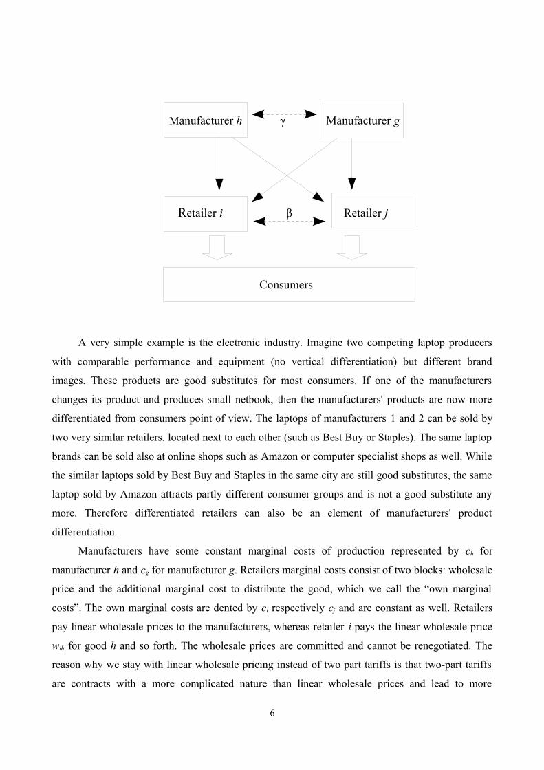
Manufacturer h γ Manufacturer g
Retailer i β Retailer j
Consumers
A very simple example is the electronic industry. Imagine two competing laptop producers
with comparable performance and equipment (no vertical differentiation) but different brand
images. These products are good substitutes for most consumers. If one of the manufacturers
changes its product and produces small netbook, then the manufacturers' products are now more
differentiated from consumers point of view. The laptops of manufacturers 1 and 2 can be sold by
two very similar retailers, located next to each other (such as Best Buy or Staples). The same laptop
brands can be sold also at online shops such as Amazon or computer specialist shops as well. While
the similar laptops sold by Best Buy and Staples in the same city are still good substitutes, the same
laptop sold by Amazon attracts partly different consumer groups and is not a good substitute any
more. Therefore differentiated retailers can also be an element of manufacturers' product
differentiation.
Manufacturers have some constant marginal costs of production represented by ch for
manufacturer h and cg for manufacturer g. Retailers marginal costs consist of two blocks: wholesale
price and the additional marginal cost to distribute the good, which we call the “own marginal
costs”. The own marginal costs are dented by ci respectively cj and are constant as well. Retailers
pay linear wholesale prices to the manufacturers, whereas retailer i pays the linear wholesale price
wih for good h and so forth. The wholesale prices are committed and cannot be renegotiated. The
reason why we stay with linear wholesale pricing instead of two part tariffs is that two-part tariffs
are contracts with a more complicated nature than linear wholesale prices and lead to more
6

problems of imperfect contracts. Beside that linear wholesale prices help the feasibility of the
model. Fix production costs in both upstream and downstream market do not change the results. For
this reason I assume fix production costs to be zero for both manufacturers and retailers without
loss of generality.
Demand Side
The demand is illustrated by a representative consumer who purchases all the goods q11, q12,
q21 and q22, whereas q12 is good 1 purchased by retailer 2 and so forth. The representative consumer
maximizes his utility function U q11, q12, q21, q22 subject to his Budget constraint y=n+qT pT.
Thereby qT=[q11, q12, q21, q22] , pT=[ p11, p12, p21, p22 ] , y is the budget of representative
consumer and n represents the numeraire. The price of numeraire is normalized to one. The
quadratic and strictly concave gross utility function is thereby:
U=nqT I a−12
qT Z q (1)
Where I is a unit vector, a is the maximum willingness to pay of a consumer for any good sold by
any retailer and the utility function is concave and Z is:
Z=[a a a a ]
Whereby δ reflects the demand effect of the rival brand sold at the rival retailer. The consumers
maximize their net utility function subject to the budget constraint y=nqT p.
a I qT−12
qT Z q− pqT
Since the Lagrangian multiplier equals one, the inverse demand system is:
p=a I−Z q
In our model where both retailers distribute products of both manufacturers, the inverse
demand function for good h sold by retailer i can be easily driven by solving the four first order
conditions:
p ih=a−qih− q jh− qig− q jg
where , ,∈[0,1 ]. It is reasonable to suppose that δ is a function of both interbrand and
intrabrand competition. With (imperfect) interbrand and intrabrand competition it is clear that δ
7

should be less than both β and γ. For feasibility reasons, we weight both of these influences in equal
proportions and assume that δ = β γ. This assumption helps specially by facilitating the derivation
of direct demands from the indirect demand functions. Also by reducing the number of variables to
just two key parameters, β and γ, we are able to present a simple graphical analysis. We would like
to notice that there is no necessary correlation, positive or negative, at the definitional level between
β and γ.
Rearranging and solving the inverse demand functions, leads to the following demand
function for good h sold by retailer i:
qhi=a 1−1−−p ih p jh pig −p jg
1−21−2 (2)
Following from the linear quadratic utility function assumed in this model, demand is ceteris
paribus higher the more differentiated manufacturer's products and retailer's services are. This is a
reasonable assumption since due to higher differentiation in upstream or downstream market, a
wider range of consumers' tastes can be served.7
2.1 Equilibrium
Downstream Market
The model is solved recursively. First we have to solve the retailers' profit maximization
problem for given wholesale prices. Each retailers maximizes his profit function
i=q ih pih−wih−ciqig pig−w ig−c i (3)
By setting his retail prices pih and pig. By inserting (2) into the profit function, we get:
πi=∑h=1
2
( pih−wih−ci)a (1−β)(1−γ)− pih+ p jhβ+ pig γ−p jgβ γ
(1−β2)(1−γ2) (4)
The profit maximizing first order conditions of retailer i is
∂πi
∂ pih=0⇔ a
1+β+γ+βγ+
ci+w ih−2 p ih+p jhβ+(2 pig−c i−wig−p jgβ)γ
(1−β2)(1−γ2)=0
∂ i
∂ pig=0⇔ a
1
wig−2 p ig p jg2 pih−wih− p jh
1−21−2=0
(5)
7 For a better illustration please refer to the example mentioned above.
8

These first order conditions lead to the equilibrium retail price of each good depending on
wholesale prices:
p ih=a 2−−22wihc iw jhc j
4−2 (6)
The retail-prices increase ceteris paribus, the higher own marginal costs and wholesale price
of the good for the retailer and for it's competitor is and it decreases the higher substitutability of
retailers' services are. The retail prices do neither depend directly on degree of substitutability
among manufacturers' products nor on the wholesale prices of the substitute good g paid by retailer
i. Later we will show that the wholesale price of any good depends on degree of interbrand
competition and the wholesale prices of the substitute good. Inserting β = 0 in (6) yields to the
standard monopoly price p ih=aw ihc i/2. On the other extreme, the better substitutes the
goods become, the more retail price approaches p ih=2wihc iw jhc j/3. As soon as
interbrand competition exceeds a certain threshold (which we will analyze later), the sales of the
retailers with the higher own marginal costs will collapse and the remaining monopolist sets prices
low enough to keep the competitor out of the market.
Substituting (6) in (2) leads to the equilibrium outputs depending on wholesale prices:
qih=a 2−−21−−2−2 wih22w ig w jhw jg1−c i2−2 −c j
4−5 241−2 (7)
The terms for qig, qjh and qjg are analogous.
Upstream Market
After solving the problem of firms in the downstream stage, we go one step back and solve
the profit maximizing problem of the upstream firms based on (7). The marginal costs of
manufacturers h and g are denoted by ch and cg respectively. In this stage the manufacturer
maximizes his profits by choosing wholesale prices taking into account that wholesale prices
influences the retail prices of the manufacturers and though the sales.
The profit of manufacturer h is:
h=wih−chqihw jh−chq jh (8)
By inserting (7) in (8), building the profit maximizing first order conditions subject to wih and wjh,
and solving them yields to:
9
w ih=a 2−−22ch−c ic gc i1
4−2 (9)
Thus if retailers have symmetric own marginal costs (ci = cj), then manufacturers have no incentive
to prices discriminate among retailers. If the manufacturers are monopolists (γ = 0), then
manufacturer h's wholesale price is (a+ch – ci)/2. The higher interbrand competition γ, the stronger
wholesale prices depend on marginal costs of the competitor and the lower equilibrium wholesale
prices are. The wholesale price does not depend directly on degree of intrabrand competition.
By inserting (9) in (6) and (7) we derive the retail prices and outputs in equilibrium
depending only on exogenous parameters such as manufacturer's costs, consumers maximum
willingness to pay and the degree of interbrand and intrabrand competition:
p ih=a− a2−2−
2chc g
2−4−2
2ci c j
4−22−(10)
q ih=a
2−22−2−
ch2−2−cg 2−24−524
−ci2−2−c j
2−24−524 (11)
If we assume that there is a monopoly in both stages (β = γ = 0), we get the standard solution
p ih=achci
4and q ih=
a−ch−ci
4. 8 The retail price converges to p ih=
2chc icgc j
3,
the tougher interbrand and intrabrand competition become (β , γ → 1).9
By calculating the prices for cournot competition in both markets we find that prices are
lower and thus output and welfare are higher under Bertrand competition which confirms the results
in the existing literature. The Cournot results can be found in the appendix.
8 If we consider the even more special case of symmetric manufacturers and symmetric retailers, then the
wholesale price in equilibrium will be for all the goods and each retailer w=a− a−c2− and the corresponding
equilibrium output for each of the goods sold by any retailer is q ih=a−c
2−1 2−1 . The common
retail price for all goods is p=a− a−c2−2− , the profits of both manufacturers are i=1− and
retailers profits are h=1−2− where =
2 a−c2
2−12−21.
The profits of manufacturers decreases as β approaches to 0.5 or as γ increases. While retailers' profits decreases
as β increases and it increases as γ increases.
9 As we mentioned above, if manufacturers/retailers are asymmetric, the demand of the weaker competitor
collapses, as soon as the difference among the marginal costs of manufacturers/retailers exceeds a certain
threshold. This threshold will be analyzed in proposition 1 in section 3.
10

Profits
In order to make the analysis of manufacturers' (retailers') profits more feasible, we assume
both firms in the downstream (upstream) market have symmetric own marginal costs cd (cu).
Substituting (9) and (11) back into (8) leads – under the assumption c i=c j=cd – to the profit
function of manufacturer h in equilibrium:
h=2 c gcdchcd −2chcd a 2−−22
2−24−221−2 (12)
Since β can only be found in the denominator of manufacturers' profit, the dependency of
manufacturers' profit on intrabrand competition can be expressed as 1/2−2. Thus the
profits of manufacturers have a U-shaped relationship with substitutability β among the retailers
services: It increases as β gets closer to the borders 0 or 1 (either if retailers' services are totally
independent or perfect substitutes) and it decreases as β gets closer to 0.5.
The reason for this U-shaped relationship is: If retailers are in perfect competition, there is no
double marginalization. The elimination of double marginalization leads ceteris paribus to lower
retail prices and hence to an increase of demand for manufacturers' goods. On the one hand, higher
differentiation of retailers' services lead to higher double marginalization effect. But on the other
hand if retailer services are more differentiated, more consumer tastes are served due to the assumed
linear-quadratic utility function and therefore the demand is ceteris paribus higher. This
countervailing effect leads to a second maximum level of upstream firms' profits with respect to the
intrabrand competition by β = 0. Thus a change in degree of intrabrand competition has a U-shaped
external effect on the profits of both manufacturers.
Inserting (9), (10) and (11) into (4) leads – under the assumption ch=cg=cu – to the profit function of retailer i in equilibrium:
i=22c icu−c jcu cicua 2−−22
2−214−22 1−2 (13)
The profits of retailers are analogous to manufacturers' profits. The dependency of
downstream firms' profits on competition in the vertically related market can be expressed
analogously to the case above as 1/2− 2. Thus, the profits of retailers have a U-shaped
relationship regarding the competition among manufacturers γ: the profits are maximized if γ is
either 0 (manufacturers are monopoly) or 1 (manufacturers' products are perfect substitutes) and it
is minimized if γ = 0.5.
11

3 Research and Development
This chapter focuses on analyzing the incentives to invest in process R&D. We assume that
only one firm in each level – in the upstream market, in the downstream market or in both markets
– can invest in process R&D. One can imagine that an inventor offers a patented innovation to the
firms, so that only one firm can use the innovation. Adding research and development to the basic
model, which already contains some complexing features, requires the simplifying tool of
considering just the R&D incentives instead of endogenizing the R&D investment. Therefore we
consider the impact of the determinants on R&D incentives devoid of specifying the amount of
R&D investment and without loss of generality. We will first start to consider R&D incentives of
manufacturer i in subsection 3.1 with symmetric downstream firms. Afterward we consider the
R&D incentives for retailer h with symmetric upstream firms in 3.2, and finally We will allow
R&D for both manufacturer h and retailer i in subsection 3.3.
3.1 R&D investments in upstream market
We assume that manufacturer h reduces his marginal costs by amount d through some fix
investments in process R&D. Before manufacturer h invests in R&D, both upstream firms h and g
have symmetric marginal costs denoted by cu. We assume that downstream firms have symmetric
“own marginal cost” as well – denoted by cd – when h invests in R&D. This assumption will be
relaxed later.
The profits of retailer are:
i=∑h=1
2
q ih p ih−wih−cd ∀ i∈{1,2} (14)
Manufacturer h reduces his marginal costs to cu - d and sets his wholesale prices according to his
reduced marginal costs. His new wholesale price is thereby:
w ih=w jh=a−cd1−cu
2−− 2 d
4−2 (15)
As long as qg is positive, the better substitutes the goods are, the “more aggressive” manufacturer h
reduces its price due to reduction in marginal costs. The reason is that when manufacturer h reduces
its prices, it gains more customers from manufacturer g the better substitutes the goods are.
Due to the new wholesale price of upstream firm h, manufacturer g reacts by decreases his
12
wholesale price as well. But since manufacturer g has higher marginal costs than its competitor h,
manufacturer g will not decrease his wholesale price as strong as manufacturer h does. The new
wholesale price of manufacturer g is therefore:
w ig=w jg=a−cd1−cu
2−− d
4−2 (16)
The better substitutes the goods are, the stronger does manufacturer g also reduces its price.
Manufacturer g reacts stronger because the consumers react stronger on prices differences the better
substitutes the goods are. As long as manufacturers are not in perfect competition, their price-
setting-behavior depends - among other factors – also on “own marginal costs” of retailers. They set
higher wholesale prices the lower the own marginal costs of retailers are.
We have to take into account that if costs are too different, only one firm can remain in the
market. If manufacturer h's price reduction exceeds a certain threshold10, the demand of the weaker
competitor collapses, because the difference among the marginal costs of manufacturers exceeds a
threshold.
Proposition 1: Manufacturer g who does not invest in R&D will produce it's product (qg >0) only if
da−cu−cd 1−2
.
Proof: See Appedix.
If γ respectively d reaches the threshold, then manufacturer h's optimal duopoly wholesale
price is the following limit price:
w ih=w jh=a−cd−a−cd−cu/ (17)
This price is low enough to keep manufacturer g out of the market. The innovation is drastic, if
d3 cucd−a . In this case, manufacturer h's monopoly price is below the limit price (17) which
keeps manufacturer g out of the market, therefore manufacturer h just sets its monopoly wholesale
price. If price reduction d exceeds the threshold d=a−cd−a−cd−cu/ to keep the competitor
out of the market but is not high enough to be drastic, manufacturer h continues limit pricing.
Manufacturer h's limit price is lower, the better substitutes the goods are. The prices setting
behavior of both manufacturers subject to manufacturer h's marginal cost reduction d is
10 Analogously we can say: “if interbrand competition exceeds a certain threshold”. The threshold for degree of
interbrand competition is =8a−cd−cu2a−cd−cud 2−acdcu−d
2a−cd−cu .
13
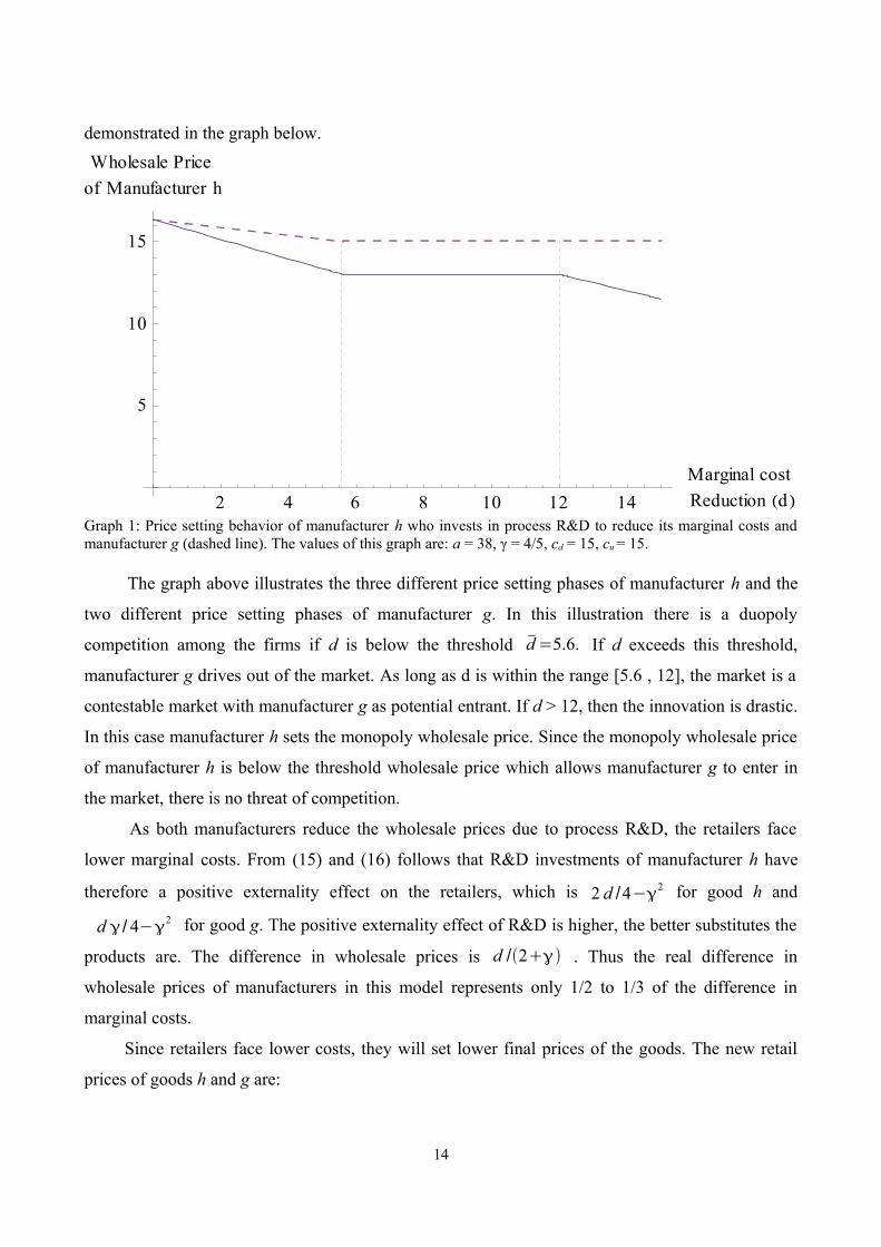
demonstrated in the graph below.
2 4 6 8 10 12 14Marginal costReduction d
5
10
15
Wholesale Priceof Manufacturer h
Graph 1: Price setting behavior of manufacturer h who invests in process R&D to reduce its marginal costs and manufacturer g (dashed line). The values of this graph are: a = 38, γ = 4/5, cd = 15, cu = 15.
The graph above illustrates the three different price setting phases of manufacturer h and the
two different price setting phases of manufacturer g. In this illustration there is a duopoly
competition among the firms if d is below the threshold d=5.6. If d exceeds this threshold,
manufacturer g drives out of the market. As long as d is within the range [5.6 , 12], the market is a
contestable market with manufacturer g as potential entrant. If d > 12, then the innovation is drastic.
In this case manufacturer h sets the monopoly wholesale price. Since the monopoly wholesale price
of manufacturer h is below the threshold wholesale price which allows manufacturer g to enter in
the market, there is no threat of competition.
As both manufacturers reduce the wholesale prices due to process R&D, the retailers face
lower marginal costs. From (15) and (16) follows that R&D investments of manufacturer h have
therefore a positive externality effect on the retailers, which is 2 d /4−2 for good h and
d / 4−2 for good g. The positive externality effect of R&D is higher, the better substitutes the
products are. The difference in wholesale prices is d /2 . Thus the real difference in
wholesale prices of manufacturers in this model represents only 1/2 to 1/3 of the difference in
marginal costs.
Since retailers face lower costs, they will set lower final prices of the goods. The new retail
prices of goods h and g are:
14

p ih=p jh=a−a−cu−cd
2−2−− 2d2−4−2
for good h and
p ig= p jg=a−a−cu−cd
2−2−− d 2−4−2
for good g.
(18)
Unless the retailers' services are perfect substitutes, they do not pass through the total
reduction of the wholesale prices to the final consumers. A price reduction of manufacturer h by the
amount of d, leads to a final price reduction of good g by d /4−22−. Thus, even the
customers who only buy product g, profit from R&D investments of firm h as well. Since
manufacturer g lowers the wholesale prices to a lesser extent than manufacturer h, the retail price of
product g is by d /22− higher than the retail price of product h. It is not only the
intensity of price reduction that depends on the degree of interbrand and intrabrand competition.
The altitude of the difference in retail prices among the goods depends on the degree of competition
in both stages as well. If manufacturer's products are very similar, manufacturer g reacts stronger to
the price reduction of his competitor; this yields ceteris paribus to a weaker difference in retail
prices. Thus, in a vertical model with interbrand and intrabrand competition and asymmetric
manufacturers, similar prices can be either a sign of intense competition among manufacturers or a
sign of low competitive pressure among retailers!
Lemma 1: Retailer's pass through rate of the lower wholesale price is1
2−.
Proof: Equilibrium (18) shows that cost reduction of manufacturer h is partly passed through to the
final price of good h with a total pass through rate2d
4−22−. In addition to this, the final
price of good g decreases by d
4−22−. These total pass through rates consist of
manufacturers' pass-through rates and retailers' pass-through rates, whereby:
– From (15) and (16) we get manufacturers' wholesale price reductions to retailers which are
2d /4−2 for good h and d /4−2 for good g.
– By dividing Manufacturers' wholesale price reductions through total pass through rates, we
get Retailers' pass through rate, which is1
2− . □
Lemma 1 shows that up to 50% of the cost differences among the manufacturers is dampened by
retailers. Through lemma 1 we can show proposition 2.
15

Proposition 2: R&D investments in upstream market lead to stronger price reductions for final consumers the higher both degree of interbrand and intrabrand competition is. This is true for all non drastic innovations.
Proof: See Appendix.
3.2 R&D in the downstream market
Retailers total marginal costs consists of two cost blocks: the wholesale prices and the own
marginal costs ci for retailer i and cj for retailer j to distribute a good. In this subsection we assume
that both retailers have identical marginal costs cd before R&D investment. Analogously to the
previous chapter I assume that one retailer – hereafter denoted by retailer i – can invest fix costs in
process R&D to reduce his own marginal costs by r.11 Therefor we express the marginal costs of
retailer j as cd and the marginal costs of retailer i as cd - r. In this subsection we assume that
manufacturers are asymmetric, hence ch ≠ cg.
The R&D investments of retailer i leads to a reduction of marginal costs of that retailer.
Hence the gross profits of retailers are:
i=∑h=1
2
q ih p ih−wih−cdr
j=∑h=1
2
q jh p jh−w jh−cd
(19)
Since retail prices are functions of r, the profit maximizing prices of retailer i are:
p ih=a 1−cd
2−
2 wihw jh −2 r4−2
, ∀ h∈{1,2} (20)
And retailer j's retail prices are:
p jh=a 1−cd
2−
2 w jhwih − r4−2
, ∀ h∈{1,2} (21)
Inserting the prices into the quantities yield
11 This could be motivated in different ways: The process R&D can be an investment in a new warehousing or
logistic system. Alternatively, one can also imagine that retailer itself is just another intermediate stage who
needs the output of upstream firms for his product, which is the input for the firms in the next stage. In this case,
the process R&D can be an investment in a new technology, which reduces the marginal costs of producing the
(intermediate-) good of the downstream firm.
16

qih=a−cd
2−21
w jh−w ih 2−22 w ig−w jg −wig
2 4−5 24 1−2
r 2−2
4−5 241
∀ h∈{1,2}
(22)
And for retailer j's output
q jh=a−cd
2−21
w ih−w jh 2−22 w jg−wig −w jg
2 4−5 24 1−2
r 2−2
4−5 24 1 (23)
Inserting (22) and (23) into (8) and maximizing subject to the wholesale prices and solving the four
first order conditions and solving the equation system leads to the wholesale prices. Manufacturers'
wholesale prices are
w ih=a−cdr 1−
2−
2ch cg
4−2 , ∀ h∈{1,2}
w jh=a−cd1−
2−
2 ch cg
4−2 , ∀ h∈{1,2}
(24)
From (24) it follows that – unless manufacturers' goods are perfect substitutes – upstream firms
price discriminate among retailers with asymmetric marginal costs, which is caused by process
R&D of retailer i. While manufacturers charge retailer j the same wholesale price as before, they
increase the wholesale price of the innovative retailer i by:
w ih r=0−w ih r =r 1−2−
(25)
If manufacturers' goods are perfect substitutes (γ=1), they simply set the wholesale prices equal to
their marginal costs, hence they will not price discriminate among the asymmetric retailers. The
more differentiated manufacturers' goods are, the more they will increase the wholesale price for
retailer i as a fraction of r. If manufacturers are monopolists (γ=0), half of the retailer's marginal
cost reduction is absorbed by higher wholesale prices of manufacturers.
The reason why the more efficient retailer faces a higher wholesale price, lies in the price
elasticity of demand = ∂ q∂ p
pq . In this case, the price elasticity of demand for the good h by
retailer i is:12
ih=p ih
a 1−1−− pih p jh pig− p jg (26)
The price elasticity increases with the retail price pih. Inserting pih from (18) in (26) (whereas d = 0)
12 We introduce for better analysis of price elasticity the assumption cg = ch = cu. This assumption is only for the
equations (26) and (27) in this subsection.
17

leads to the price elasticity depending on the external variables:
ih=cdcua 3−2−−2a−cd−cu1−1−
(27)
The lower the own marginal costs (cd) of the distributing retailer is, the lower is price elasticity of
demand. Thus, the price elasticity of demand is lower for the good sold to the retailer who invests in
process R&D and has lower marginal costs. Therefor the manufacturers set a higher wholesale price
for the more efficient retailer and do not change the wholesale price for the less efficient retailer,
which absorbs a part of the inequality of retailers.
After analyzing the effect of retailer i's process R&D on manufacturers' wholesale-price-
setting, we analyze the effect on final prices. From substituting back (24) into (21) we get the retail
prices depending on exogenous variables only:
p ih=a−a−cd
2−2−
2ch c g
2−4−2− 2 r4−22−
∀ i∈{1,2} (28)
By inserting (24) into (20) shows the impact of retailer i's process R&D on retailer j's final prices in
dependence of exogenous parameters only:
p jh=a−a−cd
2−2−
2ch c g
2−4− 2− r4−22−
∀ i∈{1,2} (29)
Although retailer j's marginal costs remain constant, it reacts on the lower costs of retailer i and sets
also lower retail prices.
Subtracting (28) from (29) shows that even though retailer j reacts on price reduction of
retailer i, retailer j's final price is byr
22− higher than retailer i's final price.
Inserting (28) and (29) in (7) leads to the quantities depending only on external variables:
q ih=a−cd
2−22−2
cg−ch 2−22−22−2
r 2−2
4−5242− 2,
∀ i∈{1,2}
(30)
The quantity sold by retailer j is
q jh=a−cd
2−22− 2
cg−ch2−22−22− 2
− r 4−5242−2
,
∀ i∈{1,2}
(31)
Similarly to the case of R&D in upstream market, retailer j will sell no goods any more if retailer i's
cost reduction is exceeds a certain threshold.
18
Proposition 3: The retailer with higher marginal costs will produce it's product under Bertrand
regime only if r2−− 2 acd 1c g ch−2cdch , where ch represents the
marginal costs of retailer with high marginal costs and cg represents competitors marginal costs.
Proof: The proof is equivalent to proof of proposition 1. □
Comparing (28) and (29) with (10) shows that retailer i reduces its price by2 r
4−22−
and the competitor reduces its price by r
4−22−. These price reductions consist of two
parts:13
– Final-price-setting of retailers depending on R&D effect
– Manufacturers' wholesale-price-setting.
The R&D effect on manufacturers' wholesale-price-setting behavior wi. and wj is already shown in
(25) and discussed above. We will briefly consider here the effect on retailers' final-price-setting
behavior. In order to see the pure mechanism of this effect only, we consider the price setting
behavior of retailers under the assumption that manufacturers set the same wholesale prices that
they were setting before R&D investments of retailer i. In this case, retailer i decreases its price by
2 r4−β2 . As we can see from retailers' profit maximizing first order conditions in (5), retailer j also
reduces its final price if its competitor reduces the price. Thus, although retailer j has no reduction
in own marginal costs, it reduces its price by r4−2 .
3.3 Impacts of interbrand and intrabrand competition on results of R&D
As we have mentioned in the introduction, there are several papers in the literature that
analyze R&D incentives depending on degree of competition among the innovating firm and its
competitor.14 One of the contributions of this paper is to analyze how R&D incentives in the
13 These price reductions are analogous to the total pass through rate of manufacturer h's R&D investment, hence it
means what proportion of the marginal cost reduction is passed through to the retail prices.
14 For example Lin and Saggi show even that investments in process R&D increase with the degree of product
differentiation.
19
upstream market do not only depend on the degree of interbrand competition, but are also subject to
the degree of intrabrand competition in the vertically related market and vice versa. In order to
analyze R&D incentives of manufacturer h, we compare how the profit increases if a fix amount of
R&D is invested depending on interbrand and intrabrand competition.
The profit of manufacturer h is:
h=2[ 2cdcu−d −cdcucdcu−d −a 2−− 2]2
2−14−221−2 (32)
The derivative of manufacturer's profit function with respect to d considers the profit gain of
manufacturer h through higher process innovation, without taking the fix costs into account.
Therefor it demonstrates the incentives of manufacturers to invest in R&D. The R&D incentives of
manufacturer h is:
∂h
∂ d=−42−22 cdcu−d cdcucdcu−d −a 2−−2
2−14−22 1−2 (33)
In order to analyze under wich value of intrabrand competition β the retailers have the most/least
incentive to invest in R&D, we differentiate (33) with respect to β. Setting the derivative equal zero
and solving for β leads to the only solution β= ½. Since the second derivative of manufacturer h's
R&D incentives is positive, the R&D incentives of the manufacturers are minimized if intrabrand
competition is at β = ½. Since the first order condition of (33) subject to β has no other value for β
in the range [0,1] than β = ½, we conclude that the R&D incentive of manufacturer i further
increases the more β is close to the extreme values zero and one.
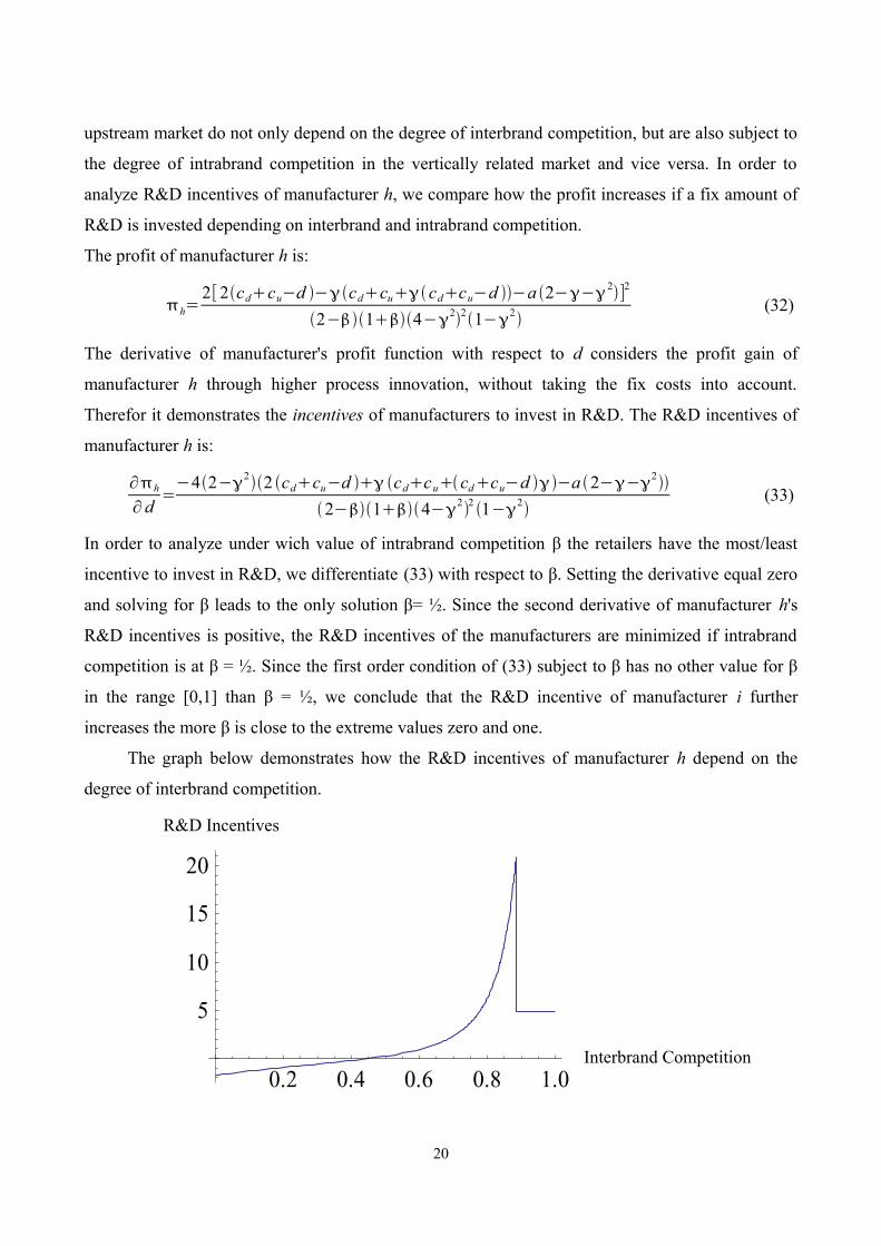
The graph below demonstrates how the R&D incentives of manufacturer h depend on the
degree of interbrand competition.
20
0.2 0.4 0.6 0.8 1.0Interbrand Competition
5
10
15
20
Incentives to invest in R&DR&D Incentives
Interbrand Competition

Graph 2: Manufacturer h's R&D incentive subject to degree of interbrand competition (derivative of manufacturer
h's profit with respect to γ) . The values of the graph are: a = 24, cd = 8, cu = 8, d = 3, β = ½. The degree of
interbrand competition γ is on the horizontal axes, and manufacturer h's R&D incentives is on the vertical axis.
In the graph we can see that If we consider low areas of γ, then the profit gain due to R&D
decreases for tougher interbrand competition, and increases for middle ranges of γ. The “turn
around point” from decreasing to increasing incentives of R&D investments subject to interbrand
competition is reached at a lower value of γ, the higher marginal cost reduction due to R&D
investments are.
In the area where interbrand competition is relaxed, an increasing interbrand competition
decreases the R&D incentives of manufacturer h, because the competitor reacts stronger and
decreases its wholesale price more due to lower wholesale price of manufacturer h. Since the
upstream firm g reacts more aggressive on the R&D investment of its competitor, the profit-gain
through R&D investment of manufacturer h is less. For this reason, in low areas of γ the R&D
incentives of manufacturer h decrease if γ increases.
If we consider middle ranges of γ – hence when competition is tough, but not tough enough to
squeeze manufacturer g out of the market – then the profit gain due to R&D is increasing and
convex for tougher interbrand competition. The reason is that under this circumstances the
wholesale price is already close to the marginal costs before the manufacturer h invests in R&D and
therefore the margins of manufacturer g are low. Manufacturer g's reaction is more “inelastic” the
lower margins of the firm are and therefor, manufacturer g's reaction on wholesale price reduction
of manufacturer h is weaker the higher γ is. Thus R&D incentives of manufacturer h increases, the
tougher interbrand competition is.
As long as the innovation is drastic, manufacturer h's incentives do not change due to a further
rise of degree of interbrand competition. In this case, the combination of cost reduction and
interbrand competition is already high enough to enable a monopoly price of the innovating firm, in
order to keep the competitor out of the market.
Proposition 4: If the combination of process innovation and interbrand competition is low, then the
R&D incentives of manufacturer i decrease ceteris paribus, if interbrand competition increases
marginally. If the combination is high, but not high enough to be a drastic innovation, an increase
of interbrand competition yields higher R&D incentives of manufacturer i. If the combination is
high enough, so that the innovation is drastic, an increasing degree of interbrand competition does
21

not change the R&D incentives of manufacturer i.
Manufacturer i has ceteris paribus the least incentives to invest in R&D, if β=½ and it has the
highest incentive if β is either zero or one.
Proof: Follows from above conclusions.
The figure below visualizes the combined relationship between manufacturer h's R&D-incentives, β
and γ.
Graph 3: R&D incentives of manufacturer h subject to the degree of interbrand and intrabrand competition. The
values of the graph are the following: a = 20, cd = 4, cu = 4, d = 2.
The graph shows the R&D incentives of manufacturer h, which is mathematically expressed
as∂πh
∂ d, subject to interbrand
∂h
∂∂ dand intrabrand
∂h
∂ ∂ dcompetition.
As we show algebraic in appendix, the R&D incentives are minimized, if β = ½ and it is
maximized, if β = 0 or if β = 1. Hence, for ∈[0.5 ;1] the R&D incentives of manufacturer h
increase if β increase and for ∈[0 ; 0.5] the R&D incentives increases the lower β is.
In low areas of γ, the profit gain due to R&D decreases for tougher interbrand competition,
and it increases in middle ranges of γ.
22

3.3 R&D in upstream and downstream market
In this subsection we solve the model for simultaneous R&D investment of a manufacturer
and a retailer, in this case manufacturer h and retailer i. Hereby, we have asymmetries in both
upstream and downstream market. In the earlier sections we have showed that if the firms in a
market are symmetric, they both profit from the R&D investment in the vertically related market. In
this section we consider what happens with the profits of both asymmetric firms, if a firm in a
vertically related market expands its investments in process R&D. First we consider the equilibrium
in the market. In the downstream stage the retailers' gross profits are
i=∑h=1
2
q ih pih−wih−cdr
j=∑h=1
2
q jh p jh−w jh−cd
(34)
Solving the downstream stage leads to the following profit maximizing retail prices:
p ih=a 1−cd
2−
2 wihw jh−2r4−2 ∀ i∈{1,2}
p jh=a 1−cd
2−
2 wihw jh− r4−2 ∀ i∈{1,2}
(35)
And the corresponding quantities are
qih=a−cd
2−21
w jh−w ih 2−22 w ig−w jg −wig
2 4−5 24 1−2
r 2−2
4−5 241
q jh=a−cd
2−21
w ih−w jh 2−22 w jg−wig −w jg
24−5 24 1−2
r 2−2
4−5 241
∀ h∈{1,2}
(36)
The profits of manufacturers are
h=∑i=1
2
qih w ih−chd
g=∑i=1
2
qig wig−cg
(37)
Building the profit maximizing first order conditions and solving the equation system leads to the
following wholesale prices:
23
w ih=(a−cd+r )(1−γ)+cu
2−γ− 2d
4−γ2 , w jh=(a−cd)(1−γ)+cu
2−γ− 2d
4−γ2 ,
w ig=(a−cd+r )(1−γ)+cu
2−γ−
γ d4−γ2 , w jg=
a−cd 1−cu
2−− d
4−2
(38)
Next we will consider the effects of R&D in one market stage on the profits of the firms in the
vertically related market by building the derivative of the firms' profits with respect to the cost
reduction in the vertically related market.
The derivative of manufacture h's profits w.r.t. R&D investments in the downstream market is:
∂h
∂ r=
2 a−cu−cd 1−2−22−21
2 r 2−21−4−52 42−21
2d 2−2
2−22−212
(39)
and manufacturer g's derivative is:
∂g
∂r=
2 a−cu−cd 1−2−22−21
2 r 2−21−4−52 42−21
− 2d 2−22−2232
(40)
The derivatives show that the process R&D investment of retailer i lead to a raise of manufacturer
h's profits but has a twofold effect on manufacturer g's profits.
The derivative of retailer i's profits with respect to R&D investments in the upstream market is:
∂ i
∂ d=1−2 qihq ig
2−4− 2 (41)
and the derivative of retailer j's profit is:
∂ j
∂ d= 2 r 2−22322−21
2a 1−cd 2−2−
2−212−21
21−d 4−32−cu1−22
2−214−221−2
(42)
If follows from (39) and (41) that the investing firms in both upstream and downstream market
always profit from a higher R&D investment in the vertically related market. It is easy to show that
the R&D investments of upstream firm h and downstream firm i mutually enforce each other. Since
we consider asymmetric firms in a market, an R&D investments in the vertically related market lead
to higher investment of the more efficient firm and the asymmetries between the firms increase.
However the effect of R&D investment in vertically related market on the unproductive firm
24

is twofold. From (40) and (42) follows that manufacturer g (retailer j) can only profit from R&D
investments of retailer i (manufacturer h) if:
– manufacturers' products (retailers' services) are sufficiently differentiated
– if retailer i's (manufacturer h's) cost reduction is big enough
– intrabrand (interbrand) competition is neither too tough nor too relaxed
4. Consumer Surplus
In this chapter we analyze the determinants of gain in consumer surplus before and after
process R&D. By subtracting consumers' expenses for the goods from the gross utility of consumers
from consuming the goods, we get the net consumer surplus. As a benchmark, we use the net
consumer surplus (CS) before R&D investments with symmetric manufacturers and retailers:
CS0=2a−cd−cu
2
2−2 12−2 1 (43)
Higher competition among manufacturers and retailers leads on the one hand to lower prices,
but on the other hand it leads to lower variety for the consumers. We build the derivative of the
consumer surplus with respect to β and γ to analyze whether one effect exceeds the other effect:
∂CS∂
=6a−cd−cu
2−3122−210
∂CS∂
=6a−cd−cu
2−3122−210
(44)
Although we have a welfare increasing element of variety in the demand function, it follows
from (44) that higher competition in any market stage leads ceteris paribus to higher consumer
surplus. If a manufacturer invests in process R&D, consumer welfare increases by
CS=2 d a−cd−cu
2−212−21 d 24−322−2 14−221−2
Consumers profit even more from manufacturer's R&D investment the higher their maximum
willingness to pay and the lower the original productivity level of manufacturers (cu) and of retailers
(cd) is.
Proposition 5: Consumers profit even more from manufacturer's R&D investment the higher
25
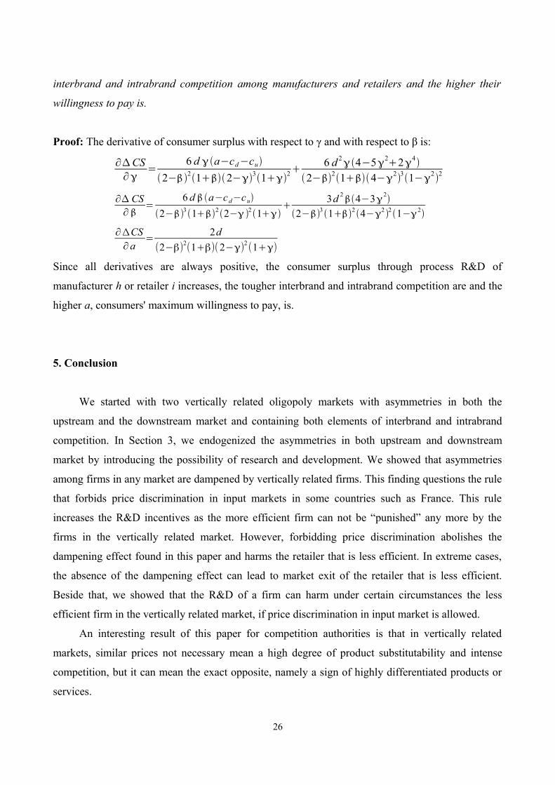
interbrand and intrabrand competition among manufacturers and retailers and the higher their
willingness to pay is.
Proof: The derivative of consumer surplus with respect to γ and with respect to β is:
∂CS∂
=6 d a−cd−cu
2−212−312 6 d 24−52242−214−231−22
∂ CS∂
=6 d a−cd−cu
2−3 12 2− 2 1 3d 2 4−3 22−3 12 4−2 2 1− 2
∂ΔCS∂a
= 2d(2−β)2(1+β)(2−γ)2(1+γ)
Since all derivatives are always positive, the consumer surplus through process R&D of
manufacturer h or retailer i increases, the tougher interbrand and intrabrand competition are and the
higher a, consumers' maximum willingness to pay, is.
5. Conclusion
We started with two vertically related oligopoly markets with asymmetries in both the
upstream and the downstream market and containing both elements of interbrand and intrabrand
competition. In Section 3, we endogenized the asymmetries in both upstream and downstream
market by introducing the possibility of research and development. We showed that asymmetries
among firms in any market are dampened by vertically related firms. This finding questions the rule
that forbids price discrimination in input markets in some countries such as France. This rule
increases the R&D incentives as the more efficient firm can not be “punished” any more by the
firms in the vertically related market. However, forbidding price discrimination abolishes the
dampening effect found in this paper and harms the retailer that is less efficient. In extreme cases,
the absence of the dampening effect can lead to market exit of the retailer that is less efficient.
Beside that, we showed that the R&D of a firm can harm under certain circumstances the less
efficient firm in the vertically related market, if price discrimination in input market is allowed.
An interesting result of this paper for competition authorities is that in vertically related
markets, similar prices not necessary mean a high degree of product substitutability and intense
competition, but it can mean the exact opposite, namely a sign of highly differentiated products or
services.
26

The model can be generalized in different ways. The assumption on agents' information (all
manufacturers know the cost functions of both retailers) is rather strong. Relaxing these
assumptions can modify the results. This paper considers a bilateral duopoly. One can extend the
model to the case which has more than two firms either in upstream or in downstream market.
Furthermore other factors such as the possibility of resale-price maintenance can also be considered
in future works.
27

Appendix
Appendix 1
Prices and quantities under Cournot Competition:
The prices in the vertical frame model are p ih=p jh=a− a 122−
12 chc g
24−2for
good h and p ig= p jg=a− a 122−
12cgch
24−2for good g. The corresponding
equilibrium outputs are q ih=q jh=a
22−1−
ch 2−2−cg 24−5 24
for good h and
q ig=q jg=a
22−1−
cg 2−2−ch24−524
for good g.
Appendix 2
Proof of Proposition 1: Substituting (15) and (16) into (7) under the assumption ci = cj = cd yields
q ig=q jg=a−cd−cu2−
2−22−2− d 2−24−524
. Setting the equation equal to zero
and solving with respect to d leads to yields to the threshold d=a−cu−cd 1−2
. Since
qig = qig sinks as d increases, d must be below this threshold in order that qig is positive. □
Appendix 3
Proof of Proposition 2: From (18) and lemma 1 it follows that the retail price of good h decreases
by2d
4−22−and retail price of good g decreases by
d 4−22−
due to process R&D
of manufacturer h. Both manufacturers and retailers pass through rates increase ceteris paribus the
tougher they are in competition.
28

Both the retail prices of good h and of good g “react” stronger on process innovation of
manufacturer h, the higher β and γ is, thus the higher the degree of interbrand and intrabrand
competition is. □
29

References
Abiru M., Nahata B., Raychaudhuri S. and Waterson, M. (1998) “Equilibrium structures in vertical
oligopoly”. Journal of Economic Behavior and Organization Vol. 37, 463 – 480.
Arrow K. (1962) ”Economic Welfare and the Allocation of Resources for Innovations”. in R.� �
Nelson ed. “The Rate and Direction of Inventive Activity”, Princeton University Press, 609-626.
Breton M., Turki A. and Zaccour G. (2004) “Dynamic Model of R&D, Spillovers, and Efficiency of
Bertrand and Cournot Equilibria”. Journal of optimization theory and applications Vol. 123, No. 1,
1–25
Chen Y. (2001) “On vertical mergers and their competitive effects”. Rand Journal of Economics
Vol. 32, 667 – 685.
Chen Z. (2003) “Dominant retailers and the countervailing-power hypothesis”, The Rand Journal of
Economics, Vol. 34 (4), 612-625
Chu A. (2009) “Effects of blocking patents on R&D: a quantitative DGE analysis”. Journal of
Economic Growth, Vol. 14, 55–78
Dobson P. and Waterson M.(1996) “Product range and interfirm competition”, Journal of
Economics and Management Strategy, Vol. 5 (3), 317-341
Dobson P. and Waterson M. (1997) “Countervailing Power and Consumer Prices”. Economic
Journal, Vol. 107, 418-430.
Dobson P. and Waterson M. (2007) “The competition effects of industry-wide vertical price fixing
in bilateral oligopoly“. International Journal of Industrial Organization, Vol. 25, 935–962
Elberfeld W. (2001) “Explaining intraindustry differences in the extent of vertical integration”.
Journal of Institutional and Theoretical Economics, Vol. 157, 465 – 477.
30
Elberfeld W. (2002) “Market size and vertical integration: Stigler's hypothesis reconsidered”.
Journal of Industrial Economics, Vol. 50, 23 – 42.
Gaudet G. and Long N. (1996) “Vertical integration, foreclosure, and profits in the presence of
double marginalization”. Journal of Economics and Management Strategy, Vol. 5, 409 – 432.
Hinloopen J. and Vandekerckhove J. (2007) “Dynamic efficiency of product market competition:
Cournot versus Bertrand”. Tinbergen Institute Discussion Paper TI 2007-097/1.
Inderst R. and Wey C. (2003) “Bargaining, mergers, and technology choice in bilaterally
oligopolistic industries”. RAND Journal of Economics, Vol. 34, 1-19.
Jaffe A. and Lerner J. (2004) “Innovation and its discontents: how our broken system is
endangering innovation and progress, and what to do about it”. Princeton University Press,
Princeton
Jansen J. (2003) “Coexistence of strategic vertical separation and integration”. International Journal
of Industrial Organization, Vol. 21, 699 – 716.
Linnemer L. (2003) “Backwards integration by a dominant firm”. Journal of Economics and
Management Strategy Vol. 12, 231 – 259.
Ordover J., Saloner G. and Salop S. (1990) “Equilibrium vertical foreclosure”. American Economic
Review Vol. 80, 127 – 142.
Kourandi F. and Vettas N. (2009) “Endogenous Spatial Differentiation with Vertical Contracting”,
mimeo, Athens Univ. of Economics and Business.
Lin P. and Saggi K. (2002) “Product differentiation, Process R&D, and the nature of market
competition”. European Economic Review 46, 201-211
31

O’Donoghue T. and Zweimuller J. (2004) “Patents in a model of endogenous growth”. Journal of
Economic Growth, Vol. 9, 81–123
Qiu L. (1997) “On the Dynamic Efficiency of Bertrand and Cournot Equilibria”. Journal of
economic theory 75, 213-229
Schumpeter J. (1934) “The theory of economic development”. Cambridge: Harvard University
Press.”
Singh, N. and Vives, X. (1984) “Price and Quantity Competition in a Di erentiated Duopoly”.ff
RAND Journal of Economics 15, 546-554.
Spence, M. (1984) “Cost Reduction, Competition, and Industry Performance”. Econometrica 52,
No. 1, 101-112.
Tirole, J. (1988): The Theory of Industrial Organization. Cambridge, MA: M.I.T. Press.
Vives, X. (1985) “On the E ciency of Bertrand and Cournot Equilibria with Product Di eren-ffi ff
tiation”. Journal of Economic Theory 36, 166-175.
Von Ungern-Sternberg T. (1996). "Countervailing Power Revisited". International Journal of
Industrial Organization 14, 507-519.
32