Federal Reserve Bank of Dallas Globalization and Monetary Policy Institute

Working Paper No. 117 http://www.dallasfed.org/assets/documents/institute/wpapers/2012/0117.pdf

Re-establishing Credibility: The Behavior of

Inflation Expectations in the Post-Volcker United States*

J. Scott Davis Federal Reserve Bank of Dallas

May 2012

Revised: February 2014

Abstract Long-term inflation expectations remained remarkably volatile in the United States for years after the well-documented switch to a more stable monetary regime in the early 1980s. This volatility cannot be explained by the standard New Keynesian model. This paper introduces a model where agents are unsure about the central bank’s commitment to their inflation target. They assume that the central bank will partially accommodate any unexpected inflation. Thus a series of high inflation observations can lead them to believe (incorrectly) that the central bank has adopted a high target. The model can match the observed volatility of long-term inflation expectations. JEL codes: D83, E31, E50

* J. Scott Davis, Federal Reserve Bank of Dallas, 2200 N. Pearl Street, Dallas, TX 75201. 214-922-5124. Scott.davis@dal.frb.org. I would like to thank conference participants at the 2013 System Macro Meeting at the Boston Fed and the 2012 Midwest Macro Meetings and seminar participants at the Hong Kong Monetary Authority for many helpful comments and suggestions. I would also like to thank Mick Devereux, Ben Keen, Enrique Martinez-Garcia, Christian Matthes, Roger Farmer, Keith Sill and Mark Wynne. The views in this paper are those of the author and do not necessarily reflect the views of the Federal Reserve Bank of Dallas or the Federal Reserve System.

The fact that there was a monetary regime change in the United States be-

ginning in 1979 with the Fed chairmanship of Paul Volcker is well documented.1

Most researchers attest that after 1980, and especially after 1984, the United

States had entered a new monetary regime with a commitment to a low and

stable inflation rate. However, even though the United States had adopted a

new monetary regime after 1984, inflation expectations, particularly long-run

inflation expectations, remained volatile for more than a decade after the end

of the Volcker disinflation. Over the period from 1984 to 1997, long-run mea-

sures of inflation expectations, like 10-year-ahead expectations, or far-forward

measures, like the 5-year-5-year forward, were around two-thirds as volatile as

observed inflation. Since 1998, that relative volatility has dropped by half and

they are now around one-third as volatile as observed inflation.

The papers mentioned earlier document the change in monetary regime

in the United States that took place in the early 1980’s. This paper will not

address that episode, instead this paper will address the reestablishment of Fed

credibility over the decades following the Volcker disinflation. The fact that the

Fed had lost credibility during the Great Inflation of the 1970’s and would have

to regain the trust of the public was foreshadowed by Fed Chairman Volcker

in Congressional testimony in 1979: "An entire generation of young adults

has grown up since the mid-1960’s knowing only inflation, indeed an inflation

that has seemed to accelerate inexorably. In the circumstances, it is hardly

surprising that many citizens have begun to wonder whether it is realistic to

anticipate a return to general price stability, and have begun to change their

behavior accordingly." (Volcker (1979) and reprinted in Malmendier and Nagel

(2013))

This paper will show how the fact that "many citizens have begun to won-

der whether it is realistic to anticipate a return to general price stability" is

evident in the dynamics of inflation expectations, particularly long-term infla-

1See Clarida, Gali and Gertler (2002), Lubik and Schorfheide (2004), Boivin and Gian-noni (2006), Stock and Watson (2007), Blanchard and Gali (2007), Blanchard and Riggi(2009), Leduc, Sill and Stark (2007), Mehra and Herrington (2008), Goodfriend and King(2005), Benati (2008), Schorfheide (2005) and Del Negro and Eusepi (2012), Bianchi (2013)among others.

2

tion expectations, after 1984. Clark and Davig (2011) show that there has been

a steady decline in both the level and the volatility of measures of long-run

inflation expectations over the past 30 years, and they attribute this to the fact

that the anchoring of inflation expectations have improved over the past few

decades, primarily due to a shift towards a more systematic and transparent

monetary policy. Using the dynamics of long-term inflation expectations to

infer something about central bank credibility, Gürkaynak, Sack and Swanson

(2005) find that in the U.S., long-run inflation expectations, proxied by far-

forward Treasury yields, respond to macroeconomic news. Far-forward rates,

which they argue are mainly composed of inflation expectations, should not

respond to macroeconomic news if long-run inflation expectations are truly

anchored. Gürkaynak, Levin and Swanson (2006) do a similar exercise but

compare the response of far-forward rates in the U.S., the UK, and Sweden to

macroeconomic news. They find that far-forward rates respond very little to

news in inflation targeting Sweden and respond the most in the U.S. Their sam-

ple contains data from the UK from both before and after the independence of

the Bank of England. They find that far-forward rates from pre-independence

UK behave more like those from the U.S., but far-forward rates from post-

independence UK behave more like Sweden. Similarly Beechey, Johannsen

and Levin (2011) use far-forward inflation expectations derived from inflation

swaps and find that far-forward inflation expectations in the U.S. are more

sensitive to current macroeconomic news than those in a number of inflation

targeting European countries. Goldberg and Klein (2005) use the response of

the yield curve to macroeconomic news to chart the establishment of European

Central Bank credibility in the first years of the euro’s existence.

Thus this paper will address two interesting questions related to the dy-

namics of inflation expectations in a post-Volcker United States. The first

is why do we observe any volatility in long-run inflation expectations in the

post-Volcker United States? The commonly cited regime shift in U.S. mone-

tary policy occurred in 1979. There was a sharp fall in inflation expectations in

the early 1980’s, but even after this switch to a stable monetary regime there

is considerable volatility in far-forward measures of inflation expectations like

3

the 5-year-5-year forward. The standard New Keynesian model cannot repro-

duce many of the dynamics of inflation expectations that we observe in the

data. Authors usually include rule-of-thumb pricing behavior, as in Gali and

Gertler (1999), sticky information, as in Mankiw and Reis (2002), or price and

wage indexation, as in Christiano, Eichenbaum and Evans (2005), to introduce

what Fuhrer (2006; 2011) refers to as "intrinsic" inflation persistence. These

features help the model explain the persistence of inflation or the dynamics

of short-run inflation expectations, but this paper will show that even with

these modifications, the standard New Keynesian model cannot account for

the volatility of far-forward measures of inflation expectations that we observe

in the data.

The second, and closely related question that this paper wishes to address

is why has there been a considerable fall in the volatility of long-run measures

of inflation expectations over the period since 1984? If the change in monetary

regime occurred in the early 1980’s, why do the volatility of long-run inflation

expectations fall much later?

To explain the persistence and variability of long-run inflation expectations,

this paper will construct a model where agents are unsure about the central

bank’s inflation target. If the central bank has limited credibility and cannot

perfectly anchor beliefs about the long-run level of inflation, then agents will

update their beliefs about the central bank’s inflation target based on past

observations of inflation. Thus a period of high inflation can lead to higher

long-run inflation expectations, which become self-fulfilling.2

A number of authors have proposed modifications to the standard New

Keynesian model to account for observed shifts in trend inflation and long-

term inflation expectations. Cogley and Sbordone (2008) estimate a model

with a role for both variable trend inflation and price indexation. They find

that variable trend inflation is responsible for the persistence of inflation in

2The mechanism is similar in spirit to the expectations trap in Albanesi, Chari andChristiano (2003). The difference is that the formal expectations traps literature is basedon discretionary policy. Here the central bank can commit (it follows a Taylor rule policyfunction), but agents are unsure about the central bank’s target and believe that the centralbank will partially accommodate any increase in inflation.

4

the data, and after accounting for variable trend inflation, price indexation

is unimportant.3 Similarly, Ireland (2007) estimates a model that allows for

variable trend inflation and finds that the Fed’s inflation target was low during

the 1950’s, rose throughout the 60’s and 70’s, and since then has fallen back

to pre-1970’s levels.

Throughout this paper we will refer to the model where agents are unsure

about the central bank’s inflation target, and thus the long-run level of infla-

tion, as the limited credibility model. This paper will show that a New Keyne-

sian model with limited credibility preforms much better than the benchmark

model with full credibility in its ability to explain the volatility of inflation

expectations that we observe in the data. We then compare the results from

model with limited credibility to the benchmark New Keynesian model with

either price and wage indexation or near permanent shocks, which are two fea-

tures that researchers use to add inflation persistence to the benchmark New

Keynesian model. The models with indexation or with near-permanent shocks

do just as well as the model with limited credibility in matching the dynam-

ics of short-run inflation expectations, but these two models preform rather

poorly in explaining the behavior of long-run inflation expectations. Only the

model with limited credibility can match the volatility and co-movement of

long-run measures of inflation expectations. We then calibrate the model to

match the observed levels of Federal Reserve credibility in the pre- and post-

1998 periods. Simply by changing the level of central bank credibility, holding

all else fixed, the model can explain nearly all of the observed changes in the

volatility of inflation expectations in the U.S. over the last few decades.

The fact that the diminished credibility of the Fed could persist for years

after the switch to a stable monetary regime in the early 1980’s is supported by

micro/survey based data on memories of past inflationary episodes. Using a

panel of responses from the World Values Survey, Ehrmann and Tzamourani

(2012) find that while memories of hyperinflation episodes never dissipate,

3In a related empirical study, Levin and Piger (2004) find that once you allow for astructural break in the level of inflation, which occurs in most countries in the late 1980’s- early 1990’s, in most countries, fluctuations in inflation are simply transitory fluctuationsaround the variable mean, and the inflation process has very little persistence.

5

memories of less dramatic high inflation episodes dissipate after about 10 years.

Malmendier and Nagel (2013) find that an individual’s expectations of inflation

are shaped by their own personal history of inflation, so memories of past

episodes of high inflation should fade as older cohorts are replaced by younger

ones. They find that the effects of the Great Inflation of the 1970’s on survey

based inflation expectations in the United States only begin to fade in the

early 1990’s.

Recently, some authors have modified the standard New Keynesian model

to say that agents don’t have complete information about the central bank’s

inflation target, and must learn this from observations of past inflation. Milani

(2007) incorporates "learning" into the standard New Keynesian model, esti-

mates the model, and finds that when learning is included, you do not need to

incorporate features like price indexation or habit formation in consumption to

get the persistence of macroeconomic variables. Similarly, Lansing (2009) con-

structs a model where agents use a Kalman filter approach to deduce whether

a shock to inflation is permanent or transitory, and he shows that this model

can reproduce the observed time-varying persistence and volatility of U.S. in-

flation. Andolfatto and Gomme (2003) and Erceg and Levin (2003) construct

models where agents are unsure about either the money growth rule or the

central bank’s inflation target, and must infer the target from past observa-

tions of inflation. They show how this learning is necessary to explain the

large output loss that accompanies a transition from a high inflation regime

(high money growth rate or high inflation target) to a low inflation regime (low

money growth rate or low inflation target). Similarly Schorfheide (2005) and

Del Negro and Eusepi (2012) estimate a DSGE model with either complete

information or a role for learning and find that the model with complete infor-

mation does well in explaining most of the historical experience in the U.S.,

but the model with learning is necessary to explain the Volcker disinflation of

the early 1980’s. Orphanides and Williams (2004; 2007) and Gaspar, Smets

and Vestin (2006; 2011) present models where agents’have imperfect informa-

tion about the parameters in the central bank’s policy rule function or where

they are unsure if a shock to inflation is transitory or permanent, and evaluate

6

optimal monetary policy in this environment of limited information/limited

credibility.

This paper will proceed as follows. Some statistics describing the behavior

of inflation expectations in the U.S. over the 30 years since the Volcker disin-

flation are presented in section 1. The theoretical model is described in section

2. The model is a cashless version of the benchmark New Keynesian model

described in Christiano, Eichenbaum and Evans (2005), but expectations are

formed using this concept of limited credibility. The calibration of the model

is discussed in section 3. Here special attention is paid to exactly how to cal-

ibrate the model to reflect historical observations of central bank credibility

and the anchoring of inflation expectations. The results from the model are

presented in section 4. Here we will examine both the path of inflation and in-

flation expectations since 1984 and simulated moments from the model to see

how the model with limited credibility preforms much better than the model

with full credibility in matching the dynamics of inflation expectations, espe-

cially long-run inflation expectations. Finally section 5 concludes with some

directions for further research.

1 The Dynamics of Inflation Expectations

In this section, we present some statistics on the dynamics of inflation expecta-

tions in the United States over the last 30 years. Furthermore, we will discuss

how there was a sharp decrease in the volatility of inflation expectations be-

tween the first and second half of this sample period.

We will consider measures of both short-run inflation expectations and

long-run inflation expectations. The three measures are: the expected change

in the price level over the next year (one-year-ahead inflation expectations,

Et (πt+1)), the expected annual inflation rate over the next ten years (10-year-

ahead inflation expectations, Et

(110

10∑i=1

πt+i

)), and the expected inflation rate

over a period beginning five years from now and ending ten years from now

(5-year-5-year forward inflation expectations, Et

(15

10∑i=6

πt+i

)).

7

Figure 1 plots U.S. inflation, one-year-ahead inflation expectations, 10-

year-ahead inflation expectations, and 5-year-5-year forward inflation expec-

tations from 1984 to 2011. The data has been demeaned. U.S. inflation is

defined as the year-over-year percentage change consumer price index (CPI),

and inflation expectations are taken from the dataset compiled by the Federal

Reserve Bank of Cleveland and described in Haubrich, Pennacchi and Ritchken

(2011). This dataset contains measures of n year ahead inflation expectations

for the U.S. for n = 1...30. Expectations are observed monthly from January

1982 to the present.

The figure shows that inflation expectations, particularly long-run mea-

sures of inflation expectations, have fallen steadily over the last 30 years. The

figure shows that there was a sharp fall in the level long-term inflation expec-

tations that occurred in the very beginning of the sample, but even after that

initial drop, long-run measures of inflation expectations have not remained

constant but have continued to fall over the last 30 years. Later, when pre-

senting the results from the New Keynesian model with full credibility and

with limited credibility, we will show that only the model with limited credi-

bility that gets improves over time can replicate the steady fall in the level of

long-run inflation expectations in the U.S. over the past 30 years.

Table 1 presents some evidence about the cross-time evolution of the volatil-

ity and persistence of inflation expectations in the United States. In the table,

the sample is split into an early sample, from 1984 to 1997, and a later sample,

from 1998 to 2011. The table also includes a third column reporting the statis-

tics from the 1998-2007 period. The first thing to notice is that the volatility

of inflation rose between the earlier sample and the later sample, but compar-

ison with the third column (the truncated late sample) shows that this rise in

inflation volatility is entirely due to the dramatic swings in inflation associated

with the global financial crisis beginning in 2008. If the post 2007 period is

excluded from the sample, the volatility of inflation fell by 20% between the

pre-1998 period and the post-1998 period. In addition to the overall fall in

inflation volatility between the early and late sample periods, there was a fall

in the relative volatility of inflation expectations. One-year-ahead inflation

8

expectations were 70% as volatile as inflation in the early sample period, but

in the later period, year-ahead expectations were only 50 − 60% as volatile

as inflation. In the early period, long-term measures of inflation expectations

were nearly two-thirds as volatile as observed inflation, but in the later period

they were only one-third as volatile as observed inflation.

In addition, there is a sharp reduction in the correlations between current

inflation and future inflation expectations between the earlier and the later

time periods. In the early period, the correlation between current inflation

and year-ahead inflation expectations was nearly 0.7, while the correlations

between current inflation and long-run measures of expectations were greater

than 0.5. In the later period (ending in 2007), the correlation between current

inflation and one-year-ahead expectations drops to about 0.3, while current

inflation and longer term measures of expectations are nearly uncorrelated.

The correlation between current inflation and 10-year-ahead expectations falls

to about 0.06, and the correlation with 5-year-5-year forward expectations falls

to 0.00.

2 The Model

The model with limited central bank credibility is based on the standard New

Keynesian model in Christiano, Eichenbaum and Evans (2005). There are mo-

nopolistically competitive intermediate goods firms that produce a differenti-

ated product that is then aggregated into a final good used for consumption,

investment and government purchases. There are also households that supply

a differentiated type of labor. Calvo (1983) pricing in both the intermediate

goods sector and the household sector gives rise to nominal wage and price

rigidities.

Due to these wage and price rigidities, a firm or a household knows that if

given the opportunity to change their price today, their new nominal price will

most likely be in place for at least a few periods into the future. Thus when

setting an optimal price or wage, price setters have to take into account not

only current conditions, but the expectation of future conditions. In the stan-

9

dard New Keynesian model, the expectation of future variables is determined

using rational expectations. We abstract from that here. Instead we assume

that agents are unsure about the central bank’s inflation target. Following a

surprise in current observed inflation, they believe that the central bank may

accommodate some of the unexpected inflation and thus may adopt a new,

higher inflation target. While the actual inflation target never changes, agents

don’t know this, and every period they update their belief about the central

bank’s target using past observations of inflation. Eventually they realize that

the central bank’s preferred measure of long-run inflation has not changed,

but their incorrect assumptions could persist for some time. Thus agents will

revise upward their beliefs about the central bank’s inflation target following

a series of high inflation observations. If agents form expectations expecting

high inflation, then these high expectations get incorporated into the price and

wage setting decisions, leading to higher inflation.

2.1 Production

Final goods, used for private consumption, government consumption, and in-

vestment are formed through a Dixit and Stiglitz (1977) aggregation of inter-

mediate goods from firms i ∈ [0 1]:

Ct + It +Gt =(∫ 1

0yt (i)

σ−1σ di

) σσ−1

(1)

where yt (i) is the quantity produced by firm i, and σ is the elasticity of sub-

stitution between intermediate goods from different firms. When considering

the results from simulations of the model, in one set of simulations we will

simulate the model under stochastic government spending shocks. There will

be more about the calibration of the exogenous process for Gt in section 3, but

the steady state value of Gt is set such that in the steady state, government

spending is 20% of GDP .

From the aggregator function in (1), the demand for the intermediate good

from firm i is:

10

yt (i) =

(Pt (i)

Pt

)−σ(Ct + It +Gt) (2)

where Pt (i) is the price set by firm i, and Pt =(∫ 1

0(Pt (i))1−σ di

) 11−σ.

The firm produces intermediate goods by combining capital and labor in

the following Cobb-Douglas production technology:

yt (i) = Atht (i)1−α kt (i)α − φ (3)

where ht (i) and kt (i) are the labor and capital employed by the firm in period

t, φ is a small fixed cost term that is calibrated to ensure that firms earn

zero profit in the steady state, and At is a stochastic productivity parameter

common to all firms.

From the firm’s cost minimization problem, the demand from firm i for

labor and capital is given by:

ht (i) = (1− α)MCtWt

(yt (i) + φ) (4)

kt (i) = αMCtRt

(yt (i) + φ)

whereWt is the wage rate, Rt is the capital rental rate andMCt = 1At

(Wt

1−α)1−α (Rt

α

)α.

Price setting by intermediate goods firms In period t, the firm will be

able to change its price with probability 1 − ξp. If the firm cannot change

prices then they are reset automatically according to Pt (i) = πIt−1Pt−1 (i),

where πIt−1 = πss, the steady state gross inflation rate. In an alternative

version of the model we will consider the case where prices are indexed to the

previous period’s inflation rate, πIt−1 = Pt−1Pt−2

.

Thus if allowed to change their price in period t, the firm will set a price

to maximize:

11

maxPt(i)

Et

( ∞∑τ=0

βτ(ξp)τλt+τ

ΠIt,t+τPt (i) yt+τ (i)−MCt+τyt+τ (i)

)where λt is the marginal utility of consumption in period t and

ΠIt,t+τ =

1 if τ = 0

Et(πIt+τ−1

)ΠIt,t+τ−1 if τ > 0

As discussed in this paper’s technical appendix, the firm that is able to

change its price in period t will set its price to:

Pt (i) =σ

σ − 1

Et

( ∞∑τ=0

βτ(ξp)τλt+τMCt+τ

(ΠIt,t+τ

)−σ(Pt+τ )

σ yt+τ

)Et

( ∞∑τ=0

βτ(ξp)τλt+τ

(ΠIt,t+τ

)1−σ(Pt+τ )

σ yt+τ

) (5)

If prices are flexible, and thus ξp = 0, then this expression reduces to:

Pt (i) =σ

σ − 1MCt

which says that the firm will set a price equal to a constant mark-up over

marginal cost.

Notice that the optimal price Pt (i) does not involve the usual rational

expectations operator, Et (·), but a modified operator Et (·).Instead of assuming that private agents know the central bank’s inflation

target with certainty, assume that agents are unsure about the inflation target

and must use past observations of inflation to update their beliefs according

to the following Kalman updating equation:

πt = πt−1 + φ(πt − Et−1 (πt)

)where πt is their belief about the inflation target at time t and πt−1 is their

belief about the target at time t− 1. Thus φ is a parameter describing agents’

beliefs about central bank accommodation. As will be seen later in this section,

12

the central bank’s actual inflation target doesn’t change, but due to limited

credibility, agents believe that the central bank may accommodate part of the

surprise in inflation by raising the target. Over time agents realize that this

is not true, the central bank did not accommodate part of the surprise in

inflation, and their beliefs about the target converge to the actual target.4

Let Ωt be the set of information about the structure of the economy, all

parameters (other than the inflation target), and the sequence of shocks to

affect the economy up to and including shocks in period t, then for any variable

xt+i for all i = 1...∞ in the model:

E (xt+i|Ωt) = E (xt+i|Ωt, πt)

and for notational simplicity define Et (xt+i) ≡ E (xt+i|Ωt).

Write the price set by the firm that can reset prices in period t as P ∗t (i)

to denote it as an optimal price. Firms that can reset prices in period t will

all reset to the same level, so P ∗t (i) = P ∗t . Substitute this optimal price into

the price index Pt =(∫ 1

0(Pt (i))1−σ di

) 11−σ. Since a firm has a probability of

1− ξp of being able to change their price, then by the law of large numbers inany period 1− ξp percent of firms will reoptimize prices. Thus the price index,Pt, can be written as:

Pt =(ξp(πIt−1Pt−1

)1−σ+(1− ξp

)(P ∗t )1−σ

) 11−σ

(6)

After combining the expression for the optimal price in (5) and the equation

4The updating equation in this model looks similar to that in Lansing (2009). There isa certain long-run level of inflation, agents don’t know what it is, and must infer it frompast observations of inflation using a Kalman updating equation. While mechanically theupdating equation is very similar to Lansing (2009), the interpretation is very different. InLansing (2009) agents observe an increase in current inflation and don’t know if the shockis permanent or transitory. In this model, agents know about the shock that led to theunexpected change in inflation, but what they are unsure about is the credibility of thecentral bank. Agents question whether the central bank will use monetary policy to returninflation to the original desired level, or if they will accommodate part of the shock. In thatway, this model is similar is spirit to those in Barro and Gordon (1983), Barro (1986), andagents’suspicion that the central bank may decide to accommodate some of an increase incurrent inflation is similar to the expectations trap models in Albanesi, Chari and Christiano(2003).

13

describing the evolution of the price index in (6), one can derive the usual New

Keynesian Phillips Curve (NKPC) that relates inflation this period to current

marginal costs and the expected value of inflation next period:

πt = βEt (πt+1) +

(1− ξp

) (1− βξp

)ξp

(mct) (7)

Notice in this Phillips curve the expectation of next period’s inflation is

arrived at when agents are unsure about the central bank’s target inflation

rate, Et (πt+1). If instead agents had full information about the central bank’s

inflation target then this NKPC simply condenses to its usual form where

Et (πt+1) replaces Et (πt+1).

In a later section we will compare the results of the model with limited

central bank credibility to the model with full information and price indexa-

tion. As discussed earlier, full price indexation implies that firms that cannot

reset their price in period t simply scale up their existing price by the previous

period’s inflation rate πt−1. In this case the NKPC becomes:

πt =1

1 + βπt−1 +

β

1 + βEt (πt+1) +

(1− ξp

) (1− βξp

)ξp (1 + β)

(mct) (8)

From equation (8) it is easy to see how the price indexation introduces

the lagged inflation term πt−1 into the Phillips curve and thus introduces

persistence into the inflation process. It is not as obvious, but the fact that the

future inflation term is denoted Et (πt+1) instead of Et (πt+1) also introduces

the lagged inflation rate and thus persistence into the Phillips curve under

limited credibility in equation (7). Recall that the expectations operator in

the model with limited credibility, Et (·), depends agent’s beliefs about thecentral bank’s inflation target, πt, which in turn depends on past observations

of inflation.

2.2 Households

Households, indexed l ∈ [0 1], supply labor, own capital, and consume from

their labor income, rental income, and interest on savings. Furthermore they

14

pay lump sum taxes to the government to finance government expenditures.

The household maximizes their utility function:

max∞∑t=0

βt[ln (Ct (l))− ψ (Ht (l))

1+σHσH

](9)

subject to their budget constraint:

PtCt (l) + PtIt (l) + Tt (l) +Bt+1 (l) (10)

= Wt (l)Ht (l) +RtKt (l) + Ξt (l) + (1 + it)Bt (l)

where Ct (l) is consumption by household l in period t, Ht (l) is the household’s

labor effort in the period, Tt (l) = PtGt (l) are the lump-sum taxes paid by

the household to finance government consumption, Bt (l) is the household’s

stock of bonds at the beginning of the period5, Wt (l) is the wage paid for the

household’s heterogenous labor supply, Kt (l) is the stock of capital owned by

the household at the beginning of the period and Ξt (l) is the share of firm

profits that are returned lump sum to the household.

The household’s capital stock, Kt (l), evolves according to the usual capital

accumulation equation:

Kt+1 (l) = (1− δ)Kt (l) + It (l)

where market clearing in the market for physical capital requires that the sum

of the physical capital stock across households is equal to the sum of physical

capital demand across firms,∫ 1

0Kt (l) dl =

∫ 1

0kt (i) di.

Each household supplies a differentiated type of labor. The function to

aggregate the labor supplied by each household into the aggregate stock of

labor employed by firms is:

Ht =

(∫ 1

0

Ht (l)θ−1θ dl

) θθ−1

(11)

5Market clearing in the bond market requires that the sum of bond holdings across allhouseholds equals zero,

∫ 10Bt (l) dl = 0.

15

where market clearing in the labor market requires that Ht =∫ 1

0ht (i) di.

Since the household supplies a differentiated type of labor, it faces a downward

sloping labor demand function:

Ht (l) =

(Wt (l)

Wt

)−θHt

2.2.1 Wage setting by households

In any given period, household l faces a probability of 1 − ξw of being able

to reset their wage. If the household cannot change its wage then it is reset

automatically according toWt (l) = πIt−1Wt−1 (l), where πIt−1 = πss, the steady

state gross inflation rate. In an alternative version of the model we will consider

the case where wages are indexed to the previous period’s inflation rate, πIt−1 =Pt−1Pt−2

.

Assume that complete asset markets exist that allow households to pool

risk. The wage rate and the labor effort will be different across households

due to nominal wage rigidity, but all other variables that appear in the house-

hold budget constraint are equal across households. Thus all households have

the same level of consumption, Ct (l) = Ct and the same marginal utility of

consumption.

If household l is allowed to reset their wages in period t they will set a wage

to maximize the expected present value of utility from consumption minus the

disutility of labor.

Et

( ∞∑τ=0

βτ (ξw)τλt+τΠ

It,t+τWt (l)Ht+τ (l)− ψ (Ht+τ (l))

1+σHσH

)Thus after technical details which are located in the appendix, the house-

hold that can reset wages in period t will choose a wage:

16

Wt (l)θσH

+1=

θ

θ − 1

1 + σHσH

ψ

Et

( ∞∑τ=0

βτ (ξw)τ(Wt+τ

ΠIt,t+τ

) θσH

+θ

(Ht+τ )1+σHσH

)Et

( ∞∑τ=0

βτ (ξw)τ λt+τΠIt,t+τ

(Wt+τ

ΠIt,t+τ

)θHt+τ

)(12)

If wages are flexible, and thus ξw = 0, this expression reduces to:

Wt (l) =θ

θ − 1

1+σHσH

ψ (Ht)1σH

λt

When wages are flexible the wage rate is equal to a mark-up, θθ−1,

multiplied by the marginal disutility of labor, 1+σHσH

ψ (Ht)1σH , divided by the

marginal utility of consumption, λt.

Notice again that when expectations of future variables are used to calcu-

late the current optimal wage, agents use the modified expectations operator,

Et (·), instead of the rational expectations operator, Et (·).Write the wage rate for the household that can reset wages in period t,

Wt (l), asW ∗t (l) to denote it as an optimal wage. Also note that all households

that can reset wages in period t will reset to the same wage rate, so W ∗t (l) =

W ∗t .

All households face a probability of (1− ξw) of being able to reset their

wages in a given period, so by the law of large numbers (1− ξw) of households

can reset their wages in a given period. Substitute W ∗t into the expression for

the aggregate wage rateWt =(∫ 1

0Wt (l)1−θ dl

) 11−θ, to derive an expression for

the evolution of the aggregate wage:

Wt =(ξw(πIt−1Wt−1

)1−θ+ (1− ξw) (W ∗

t )1−θ) 11−θ

In the model with limited credibility, the New Keynesian Phillips Curve

relating wage inflation this period to expected future wage inflation and the

marginal disutility of labor this period is given by:

17

πwt = βEt(πwt+1

)+

(1− ξw) (1− βξw)

ξw

(σH

θ + σH

)(1

σHHt − Λt − wt

)where πwt = Wt+1

Wt− 1.

If wages that could not be changed in a given period were reset using the

previous period’s inflation rate then the New Keynesian Phillips curve would

be:

πwt = πt−1−βπt+βEt(πwt+1

)+

(1− ξw) (1− βξw)

ξw

(σH

θ + σH

)(1

σHHt − Λt − wt

)Just as before in the Phillips curve with price inflation, persistence is added

to the model with indexation by the presence of the lagged inflation rate in

the Phillips curve equation. In the model with limited credibility, the lagged

inflation rate has an effect on the stock of central bank credibility and thus

on Et(πwt+1

). The full derivation of both Phillips curves is presented in the

appendix.

2.3 Monetary Policy

The monetary policy instrument is the short-run risk free rate, it, which is

determined by the central bank’s Taylor rule function:

it+1 = iss + θi (it−1 − iss) + (1− θi) (θp (πt − π) + θyyt) +mt (13)

where yt = GDPtGDPt

−1, where GDPt is the level of GDP at time t in an economy

with the same structure as the one just described and subject to the same

shocks, only there are no price or wage frictions, ξp = ξw = 0, and mt is

an exogenous monetary policy shock. π is the central bank’s inflation target,

which is fixed and is not known by the private agents in the economy.6

6The transitory money supply shock mt is needed to reconcile agents’(incorrect) beliefsabout the central bank’s inflation target with their observation of the nominal risk-free rate,the inflation rate, and the output gap. If the observed risk-free rate was set based on an

18

3 Calibration

The various parameters used in the model and their values are listed in table

2. The first five parameters, the discount factor, capital’s share of income, the

capital depreciation rate, the elasticity of substitution across varieties from dif-

ferent firms, the elasticity of substitution between labor from different house-

holds, and are all set to values that are commonly found in the literature.

The next two parameters are the Calvo wage and price stickiness parame-

ters. The wage and price stickiness parameters are set to 0.75, implying that a

household expects to change their wage and firms expect to change their prices

once a year. We use the standard Taylor rule parameters for the parameters

in the monetary policy function. The central bank places a weight of 0.5 on

the output gap, 1.5 on the inflation rate, and 0.9 on the lagged interest rate.

3.1 Calibrating the anchoring of the target

In the version of the model where long-run inflation expectations are perfectly

anchored, φ = 0. In the version of the model with limited credibility, φ > 0,

implying that agents believe the central bank will partially accommodate any

unexpected increase in inflation. Of course, this model is used to consider the

behavior of inflation expectations after the Volcker disinflation, so we assume

that there is no actual accommodation, but it takes a while for the Fed to earn

credibility and convince agents that φ should be zero.

Assume that agents have in mind the following simple model when deter-

mining the φ parameter. Quarter-over-quarter inflation follows a simple AR(1)

process:

πt = ρπt−1 + υt

where ρ is the autoregressive parameter, which agents simply estimate from

the data, and υt are innovations to inflation. Agents believe that a share φ

inflation target of π and yet agents believe that the target is πt, then they believe that whatthey are seeing is a purely transitory monetary shock mt = (1− θi) (θp (πt − π)).

19

of this shock will be accommodated, and thus agents believe that the central

bank’s inflation target, πt, follows a unit root process and in period t will

increase by φυt:

πt = πt−1 + φυt

Since the inflation target is unobservable, agents construct a series for πtfrom an H-P filtered series of πt. Thus given the series of actual inflation and

agent’s beliefs about the target:7

φ =

√var (πt − πt−1)

var (πt − ρπt−1)

Assume that agents calculate these variances with a 10-year rolling win-

dow. Using a panel of responses from the World Values Survey, Ehrmann

and Tzamourani (2012) find that while memories of hyperinflation episodes

never dissipate, memories of less dramatic high inflation episodes dissipate af-

ter about 10 years. Thus, we assume that when using past observations of

actual and trend inflation to form their beliefs about the credibility of the

central bank and the anchoring of inflation expectations, agents consider the

behavior of actual and trend inflation over the past 10 years. This assump-

tion is consistent with the evidence in Malmendier and Nagel (2013) who find

that an individual’s expectations of inflation are shaped by their own personal

history of inflation, so memories of past episodes of high inflation should fade

as older cohorts are replaced by younger ones. They argue that the effects of

the Great Inflation of the 1970’s on survey based inflation expectations in the

7As discussed earlier, the updating equation in this model looks very similar to that inLansing (2009), but the interpretation is different. In Lansing (2009), there is a shock tothe transitory component of inflation and a shock to the trend level of inflation. Theseshocks are i.i.d. Agents cannot observe which shock is responsible for the observed increasein inflation, so they must update their beliefs about the trend level of inflation using aKalman updating parameter that minimizes the means square forecast error given the twounobservable i.i.d. shocks. In this model, agents observe the original shock, but they believethat the central bank will partially accommodate that shock. The updating equation in thismodel has to do with limited central bank credibility and doubts about the commitment toan inflation target, not uncertainty about shocks.

20

United States only begin to fade in the early 1990’s.

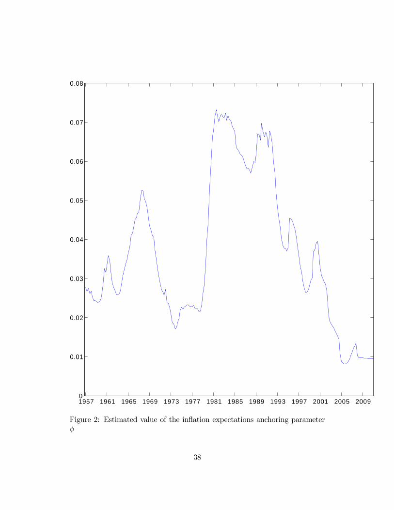
Agent’s beliefs about the credibility of the central bank, φ, calculated with

a 10-year moving window, are presented in figure 2. The figure shows that

φ increased greatly during the late 1970’s and peaked at close to 0.08 in the

early 1980’s. This implies that whenever agents observed a 1 percentage point

increase in unexpected inflation, they would assume that the central bank

would partially accommodate this by raising the inflation target by 0.08 per-

centage points. The figure also shows that φ remained high throughout the

1980’s, and only began to fall in the early 1990’s. The φ parameter had an

average value of 0.060 over the period 1984 to 1997 and an average value of

0.019 over the period 1998 to 2011. The figure shows that now the φ para-

meter is less than 0.01, meaning that beliefs about the anchoring of the Fed’s

inflation target have nearly reached the level consistent with full credibility.

However, during the 1980’s and into the early 1990’s, Fed credibility was sig-

nificantly lower, and as will be seen in the next section, only the model with

limited credibility can explain the dynamics of inflation expectations, partic-

ularly long-term measures of inflation expectations, observed throughout the

1984 to 2011 period.

3.2 Shock Processes

In the next section, we will examine the responses of inflation expectations to

both productivity and government spending shocks. For simplicity, we only

consider the effect of one shock at a time, and we assume that each shock

follows an AR(1) process with an autoregressive coeffi cient of 0.9. In one

alternative version in the next section we will consider the case where the

shock is nearly permanent with an autoregressive coeffi cient of 0.999.

Since the model is solved with a first-order approximation around the

steady state, and only one shock is active at any time, the variance of the

shock doesn’t matter for most of the dynamics in the model. To ease the

comparison between the model and the data, the variance of each shock is cal-

ibrated so that the standard deviation of inflation in the model with limited

21

credibility is 1.05%, which the same as that in the U.S. during the pre-1998

period, as seen in table 1.

4 Results

Figure 3 plots the level of inflation and inflation expectations in the United

States from 1984 to 2011. The figure plots the levels of inflation and inflation

expectations observed in the data (the data has been demeaned), as well as

the results from two simulations of the model. One set of simulation results

is from the limited credibility model, and one is from the model with full

credibility and full price and wage indexation. The sequences of productivity

shocks driving the two simulations have been backed out of the of the model

and are the sequences of productivity shocks that enable the model to exactly

match the observed path of inflation (and thus the lines in the top left hand

plot in the figure overlap by construction). Then with the sequence of shocks

we can test how well the model is able to track the observed path of inflation

expectations from 1984 to 2011.

Figure 3 shows that the model with limited credibility tracts the path of

inflation expectations remarkably well. The model is able to replicate the

steady decline in the level of long-term measures of inflation expectations over

this period. This is in stark contrast to the model with full credibility and full

price and wage indexation. The model with full credibility cannot replicate

the dynamics of long-term measures of inflation expectations observed in the

data.

From these simulations of the model where the sequences of shocks have

been set such that the model can exactly match the observed path of inflation

over the period 1984 to 2011, the correlation between the path of one-year-

ahead inflation expectations in the data and those in the model with full

credibility is 0.41, but the correlation between the path of one-year-ahead in-

flation expectations in the data and those in the model with limited credibility

is 0.83. Similarly, the correlation between 10-year-ahead inflation expectations

in the data and those in the model with full credibility is 0.12, but the corre-

22

lation with those in the model with limited credibility is 0.92. The correlation

between the 5-year-5-year froward expected inflation rate in the data and that

in the model with full credibility is −0.12, but the correlation between the 5-

year-5-year forward in the data and that in the model with limited credibility

is 0.91.

4.1 Moments from model simulations

The volatility and persistence of current and expected inflation taken from

simulations of the model under productivity shocks is presented in table 3.

The table presents simulated moments from four versions of the model. The

benchmark version of the model with full credibility, no price and wage in-

dexation, and non-permanent shocks, the version of the model with limited

credibility, the version of the model with full price and wage indexation, and

the version of the model where the exogenous shock follows close to a unit root

process.

The table is meant to compare the model with limited credibility with

the other modifications of the New Keynesian model authors have proposed

to raise the persistence of inflation. First, from the table it is clear that all

three modifications, limited credibility, indexation, and permanent shocks, in-

crease raise the relative volatility of One-year-ahead inflation expectations, and

they improve the model’s ability to match the positive co-movement between

current inflation and inflation expectations (particularly long-run inflation ex-

pectations).

However, the models with price and wage indexation or permanent shocks

fail to match the relative volatility of long-term inflation expectations. As is

shown in table 1, in the United States in the 1980’s long-run inflation expec-

tations, either the 10-year-ahead expected inflation rate or the 5-year-5-year

forward expected inflation rate are around half as volatile as current inflation.

In the benchmark New Keynesian model they are around a tenth as volatile

as current inflation. Adding intrinsic or inherited inflation persistence does go

some way towards explaining the volatility of 10-year-ahead expectations, but

23

these two modifications fail to raise the relative volatility of the 5-year-5-year

forward expected inflation rate. Introducing price and wage indexation or a

near permanent shock process actually leads to a fall in the relative volatility

of the 5-year-5-year forward rate. Only the model with limited credibility,

parameterized to match the anchoring of inflation expectations observed in

the United States, can produce the observed relative volatility of long-run

expected inflation.

Table 4 presents the same model simulation results, only now the model

is driven by government spending shocks instead of productivity shocks. The

results are similar, just as in the case where the model is driven by productivity

shocks, only the version of the model with limited credibility can replicate the

volatility of long-run inflation expectations. Just as before, the versions of the

model with indexation or near permanent shocks bring a slight improvement

in the ability of the New Keynesian model to match the relative volatility of

10-year-ahead inflation expectations, but do not begin to explain the volatility

of the 5-year-5-year forward rate.

Comparing changes in credibility Table 5 presents the results from two

simulations of the limited credibility model, one where the φ parameter has

been set to match the observed credibility in the data from 1984 to 1997,

φ = 0.060, and one where the φ parameter has been set to match the observed

credibility in the post-1998 data, φ = 0.019. The first set of columns presents

the results from simulations to the model under productivity shocks, the sec-

ond set of columns presents simulated responses under government spending

shocks.

Thus table 5 is meant to show whether or not the observed changes in

the dynamics of U.S. inflation expectations from the 1980’s to today can be

explained by changes in central bank credibility, holding all else constant.

The first thing to notice is that the model can explain the fall in U.S.

inflation volatility between the 1984 to 1997 period to the 1998 to 2007 period.

In the data, U.S. inflation volatility fell by 18% over this period. The model

predicts that a change in the φ parameter, holding all else fixed, should result

24

in a 22% fall in inflation volatility.

The change in anchoring can also explain the fall in the relative volatility

of various measures of expected inflation. In the data, the relative volatility

of One-year-ahead inflation expectations fell by about 20% and that for long-

run expectations fell by 40%. The model predicts that the relative volatility

of one-year-ahead expectations should fall by about 20% and the volatility of

long-run expectations should fall by 50%.

In the data the contemporaneous correlation between observed inflation

and long-term inflation expectations fell by 50 percentage points. The models

predict that the change in the anchoring parameter φ, holding all else con-

stant, should result in a 40-50 percentage point fall in the correlation between

inflation and long-term measures of inflation expectations.

5 Summary and conclusion

This paper provides a mechanism through which past observations of inflation

can influence the public’s perception of the central bank’s inflation target and

thus can influence inflation expectations into the future. This paper shows how

this mechanism can lead to an increase in the volatility of inflation expectations

in the benchmark New Keynesian model. Other features added to the standard

New Keynesian model, like price and wage indexation, can improve on the

model’s ability to explain the volatility and persistence of current inflation and

short-run inflation expectations, but only the model with limited credibility

can match the volatility of long-run inflation expectations that we see in the

data.

This concept of limited central bank credibility gives rise to two interesting

directions for further research. The first is in an open economy. As described

in the first paragraph of the introduction, when Milton Friedman said that

"inflation is always and everywhere a monetary phenomenon", he was care-

ful to qualify that inflation is a sustained increase in the general price level.

Exogenous shocks, like an increase in commodity prices, could lead to a transi-

tory increase in the price level, but a sustained increase over the long run must

25

be driven by monetary policy, or at least the public’s perception of monetary

policy.

Thus an interesting extension of this limited credibility model to an open

economy would be to consider how foreign shocks that cause a transitory

increase in domestic inflation might affect inflation expectations when the

central bank has limited credibility. In this case the transitory increase in

prices due to the foreign shock could have a long-lasting effect on domestic

inflation.8

The second, and closely related direction for further research, relates to the

optimal conduct of monetary policy when the central bank’s stock of credibility

is limited. Orphanides and Williams (2004; 2007) and Gaspar, Smets and

Vestin (2006; 2011) present models where agents’have imperfect information

about the parameters in the central bank’s policy rule function or where they

are unsure if a shock to inflation is transitory or permanent. These models

all show that in this environment, the central bank should be more aggressive

when responding to changes in inflation.

Posen (2011) argues that the central bank’s reaction to a transitory in-

crease in prices should depend on the anchoring of inflation expectations. If

agents’ beliefs about the inflation target are very sensitive to the observed

inflation rate (in terms of the model, a high φ parameter) then then central

bank will want to be very aggressive in responding to transitory increases in

inflation, but as expectations become better anchored and agents’beliefs be-

come less responsive to the observed inflation rate (a lower φ parameter) then

the central bank may not want to be as aggressive in responding to transitory

movements in prices. Thus an interesting direction for further research would

be to quantify how the central bank’s optimal monetary policy depends on

8In a similar vein, a number of papers have shown that the effect of transitory oil priceshocks has diminished over time and go on to argue that one of the reasons for this changeis improved central bank credibility (e.g. Blanchard and Gali (2007), Leduc, Sill and Stark(2007), Mehra and Herrington (2008), Blanchard and Riggi (2009), Evans and Fisher (2011))However, these papers generally divide the sample into pre- and post-1979 periods. Giventhat the reestablishment of Fed credibility occurred much later, an interesting direction forfurther research would be to study the effect of oil price shocks on U.S. inflation pre- andpost-1997.

26

this "anchoring" of inflation expectations.

27

References

Albanesi, Stefania, V.V. Chari, and Lawrence J. Christiano. 2003.“Expectations Traps and Monetary Policy.”Review of Economic Studies,70: 715—741.

Andolfatto, David, and Paul Gomme. 2003. “Monetary policy regimesand beliefs.”International Economic Review, 44: 1—30.

Barro, Robert J. 1986. “Reputation in a model of monetary policy withincomplete information.”Journal of Monetary Economics, 17: 3—20.

Barro, Robert J., and David B. Gordon. 1983. “A Positive Theory ofMonetary Policy in a Natural Rate Model.”Journal of Political Economy,91(4): 589—610.

Beechey, Meredith J., Benjamin K. Johannsen, and Andrew T.Levin. 2011. “Are Long-Run Inflation Expectations More Firmly An-chored in the Euro-Area Than in the United States?” American Eco-nomic Journal: Macroeconomics, 3: 104—129.

Benati, Luca. 2008. “Investigating Inflation Persistence Across MonetaryRegimes.”Quarterly Journal of Economics, 123(3): 1005—1060.

Bianchi, Francesco. 2013. “Regime Switches, AgentsŠ Beliefs, and Post-World War II U.S. Macroeconomic Dynamics.”Review of Economic Stud-ies, 80: 463—490.

Blanchard, Oliver J., and Jordi Gali. 2007. “The Macroeconomic Effectsof Oil Shocks: Why Are the 2000s So Different From the 1970s?”NBERWorking Paper no. 13368.

Blanchard, Oliver J., and Marianna Riggi. 2009. “Why Are the 2000s SoDifferent From the 1970s? A Structural Interpretation of Changes in theMacroeconomic Effects of Oil Prices.”NBER Working Paper no. 15467.

Boivin, Jean, and Marc P. Giannoni. 2006. “Has monetary policy becomemore effective?”Review of Economics and Statistics, 88(3): 445—462.

Calvo, Guillermo A. 1983. “Staggered Prices in a Utility-MaximizingFramework.”Journal of Monetary Economics, 12: 383—398.

28

Christiano, Lawrence J., Martin Eichenbaum, and Charles L. Evans.2005. “Nominal Rigities and the Dynamic Effects of a Shock to MonetaryPolicy.”Journal of Political Economy, 113: 1—45.

Clarida, Richard, Jordi Gali, and Mark Gertler. 2002. “A simple frame-work for monetary policy analysis.” Journal of Monetary Economics,49: 879—904.

Clark, Todd E., and Troy Davig. 2011. “Decomposing the DecliningVolatility of Long-Term Inflation Expectations.” Journal of EconomicDynamics and Control, 35(7): 981—999.

Cogley, Timothy, and Argia M. Sbordone. 2008. “Trend inflation, in-dexation, and inflation persistence in the new Keynesian Phillips Curve.”American Economic Review, 98(5): 2101—2126.

Del Negro, Marco, and Stefano Eusepi. 2012. “Fitting observed inflationexpectations.”Journal of Economic Dynamics and Control, forthcoming.

Dixit, Avinash K., and Joseph E. Stiglitz. 1977. “Monopolistic Com-petition and Optimum Product Diversity.”American Economic Review,67: 297—308.

Ehrmann, Michael, and Panagiota Tzamourani. 2012. “Memories ofhigh inflation.”European Journal of Political Economy, 28(2): 174—191.

Erceg, Christopher J., and Andrew T. Levin. 2003. “Imperfect credibil-ity and inflation persistence.”Journal of Monetary Economics, 50: 915—944.

Evans, Charles L., and Jonas D.M. Fisher. 2011. “What Are the Impli-cations of Rising Commodity Prices for Inflation and Monetary Policy?”Chicago Fed Letter, , (no. 286).

Fuhrer, Jeffrey C. 2006. “Intrinsic and Inherited Inflation Persistence.”In-ternational Journal of Central Banking, 2(3): 49—86.

Fuhrer, Jeffrey C. 2011. “Inflation Persistence.”In Handbook of MonetaryEconomics. Vol. 3A, , ed. Benjamin M. Friedman and Michael Woodford,423—486. North Holland.

Gali, Jordi, and Mark Gertler. 1999. “Inflation dynamics: A structuraleconometric approach.”Journal of Monetary Economics, 44: 195—222.

29

Gaspar, Vitor, Frank Smets, and David Vestin. 2006. “Adaptive Learn-ing, Persistence, and Optimal Monetary Policy.”Journal of the EuropeanEconomic Association, 4: 376—385.

Gaspar, Vitor, Frank Smets, and David Vestin. 2011. “Inflation Ex-pectations, Adaptive Learning, and Optimal Monetary Policy.”In Hand-book of Monetary Economics. Vol. 3B, , ed. Benjamin M. Friedman andMichael Woodford, 1055—1096. North Holland.

Goldberg, Linda S., and Michael W. Klein. 2005. “Establishing Cred-ibility: Evolving Perceptions of the European Central Bank.” FederalReserve Bank of New York Staff Report No. 231.

Goodfriend, Marvin, and Robert G. King. 2005. “The Incredible VolckerDisinflation.”Journal of Monetary Economics, 52(5): 981—1015.

Gürkaynak, Refet S., Andrew T. Levin, and Eric T. Swanson. 2006.“Does Inflation Targeting Anchor Long-Run Inflation Expectations? Ev-idence from Long-Term Bond Yields in the U.S., U.K., and Sweden.”Federal Reserve Bank of San Francisco Working Paper no. 2006-09.

Gürkaynak, Refet S., Brian Sack, and Eric T. Swanson. 2005. “TheSensitivity of Long-Term Interest Rates to Economic News: Evidence andImplications for Macroeconomic Models.”American Economic Review,95(1): 425—436.

Haubrich, Joseph G., George Pennacchi, and Peter Ritchken. 2011.“Inflation Expectations, Real Rates, and Risk Premia: Evidence fromInflation Swaps.”Federal Reserve Bank of Cleveland Working Paper no.11-07.

Ireland, Peter N. 2007. “Changes in the Federal Reserves’s inflation tar-get: Causes and consequences.”Journal of Money, Credit, and Banking,39: 1851—1882.

Lansing, Kevin J. 2009. “Time Varying U.S. Inflation Dynamics andthe New Keynesian Phillips Curve.” Review of Economic Dynamics,12(2): 304—326.

Leduc, Sylvain, Keith Sill, and Tom Stark. 2007. “Self-Fulfilling Ex-pectations and the Inflation of the 1970s: Evidence From the LivingstonSurvey.”Journal of Monetary Economics, 54: 433—459.

30

Levin, Andrew T., and Jeremy M. Piger. 2004. “Is inflation persistenceintrinsic in industrial economies.”ECB Working Paper no. 334.

Lubik, Thomas, and Frank Schorfheide. 2004. “Testing for Indetermi-nacy: An Application to U.S. Monetary Policy.” American EconomicReview, 94(1): 190—217.

Malmendier, Ulrike, and Stefan Nagel. 2013. “Learning from InflationExperiences.”mimeo.

Mankiw, N. Gregory, and Ricardo Reis. 2002. “Sticky information versussticky prices: A proposal to replace the New Keynesian Phillips Curve.”Quarterly Journal of Economics, 117(4): 1295—1328.

Mehra, Yash P., and Christopher Herrington. 2008. “On the Sourcesof Movements in Inflation Expectations: A Few Insights From aVAR Model.”Federal Reserve Bank of Richmond Economic Quarterly,94(2): 121—146.

Milani, Fabio. 2007. “Expectations, learning and macroeconomic persis-tence.”Journal of Monetary Economics, 54: 2065—2082.

Orphanides, Athansios, and John C. Williams. 2004. “Imperfect Knowl-edge, Inflation Expectations, and Monetary Policy.” In The Inflation-Targeting Debate. , ed. Ben S. Bernanke and Michael Woodford, 201—246.University of Chicago Press.

Orphanides, Athansios, and John C. Williams. 2007. “Robust mone-tary policy with imperfect knowledge.”Journal of Monetary Economics,54: 1406—1435.

Posen, Adam. 2011. “The Soft Tyranny of Inflation Expectations.”Interna-tional Finance, 0: 1—26.

Schorfheide, Frank. 2005. “Learning and Monetary Policy Shifts.”Reviewof Economic Dynamics, 8: 392—419.

Stock, James H., and Mark W. Watson. 2007. “Why Has U.S. InflationBecome Harder to Forecast?” Journal of Money, Credit, and Banking,39(1): 3—33.

Volcker, Paul. 1979. “Statement Before the Joint Economic Committee of theU.S. Congress. October 17, 1979.”Federal Reserve Bulletin, 65(11): 888—890.

31

Table 1: Volatility and Persistence of inflation and inflation expectations.Inflation expectations data is from the dataset produced by the Federal ReserveBank of Cleveland and described in Haubrich,Pennacchi, and Ritchken (2011)

U.S. Data1984− 1997 1998− 2011 1998− 2007

Standard deviation (%) πt 1.05 1.30 0.86

Standard deviation Et (πt+1) 0.68 0.58 0.56

relative to πt 110

10∑i=1

Et (πt+i) 0.64 0.36 0.39

Et

(15

10∑i=6

πt+i

)0.59 0.32 0.36

Correlation with πt Et (πt+1) 0.68 0.46 0.28

110

10∑i=1

Et (πt+i) 0.54 0.21 0.06

Et

(15

10∑i=6

πt+i

)0.51 0.15 0.00

Correlation with πt−1 Et (πt+1) 0.65 0.31 0.48

110

10∑i=1

Et (πt+i) 0.54 0.14 0.08

Et

(15

10∑i=6

πt+i

)0.51 0.09 −0.01

Autocorrelation πt 0.86 0.62 0.58Et (πt+1) 0.86 0.55 0.33

110

10∑i=1

Et (πt+i) 0.91 0.88 0.79

Et

(15

10∑i=6

πt+i

)0.90 0.88 0.78

32

Table 2: Parameter ValuesSymbol Value Description

β 0.99 discount factorα .36 capital share in production of value addedδ 0.025 capital depreciation rateσ 10 elasticity of substitution (eos) across varieties from different firmsθ 21 eos between labor from different householdsξp 0.75 probability that a firm cannot reset pricesξw 0.75 probability that a household cannot reset wagesθp 1.5 coeffi cient on inflation in the Taylor ruleθy .5 coeffi cient on the output gap in the Taylor ruleθi .9 coeffi cient on the lagged interest rate in the Taylor ruleφ 0.06 or 0.019 parameter describing agents’beliefs about central bank accommodation

33

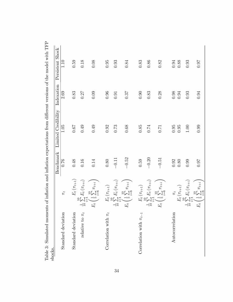
Table3:Simulatedmomentsofinflationandinflationexpectationsfrom

differentversionsofthemodelwithTFP

shocks.

Benchmark

LimitedCredibility

Indexation

PersistentShock

Standarddeviation

πt

0.76

1.05

2.69

1.10

Standarddeviation

Et(π

t+1)

0.48

0.67

0.83

0.59

relativetoπt

1 10

10 ∑ i=1

Et(π

t+i)

0.16

0.49

0.27

0.18

Et

( 1 5

10 ∑ i=6

πt+i)

0.14

0.49

0.09

0.08

Correlationwithπt

Et(π

t+1)

0.80

0.92

0.96

0.95

1 10

10 ∑ i=1

Et(π

t+i)

−0.

110.

730.

910.

93

Et

( 1 5

10 ∑ i=6

πt+i)

−0.

520.

680.

370.

84

Correlationwithπt−

1Et(π

t+1)

0.59

0.85

0.90

0.83

1 10

10 ∑ i=1

Et(π

t+i)

−0.

200.

740.

830.

86

Et

( 1 5

10 ∑ i=6

πt+i)

−0.

510.

710.

280.

82

Autocorrelation

πt

0.92

0.95

0.98

0.94

Et(π

t+1)

0.80

0.95

0.94

0.88

1 10

10 ∑ i=1

Et(π

t+i)

0.99

1.00

0.93

0.93

Et

( 1 5

10 ∑ i=6

πt+i)

0.97

0.99

0.94

0.97

34

Table4:Simulatedmomentsofinflationandinflationexpectationsfrom

differentversionsofthemodelwith

governmentspendingshocks.

Benchmark

LimitedCredibility

Indexation

PersistentShock

Standarddeviation

πt

0.74

1.05

2.96

1.14

Standarddeviation

Et(π

t+1)

0.57

0.74

0.88

0.36

relativetoπt

1 10

10 ∑ i=1

Et(π

t+i)

0.21

0.47

0.35

0.14

Et

( 1 5

10 ∑ i=6

πt+i)

0.21

0.45

0.14

0.12

Correlationwithπt

Et(π

t+1)

0.93

0.97

0.98

0.79

1 10

10 ∑ i=1

Et(π

t+i)

0.10

0.81

0.90

−0.

14

Et

( 1 5

10 ∑ i=6

πt+i)

−0.

520.

680.

45−

0.46

Correlationwithπt−

1Et(π

t+1)

0.81

0.93

0.94

0.57

1 10

10 ∑ i=1

Et(π

t+i)

0.01

0.81

0.84

−0.

22

Et

( 1 5

10 ∑ i=6

πt+i)

−0.

530.

710.

37−

0.45

Autocorrelation

πt

0.93

0.96

0.99

0.89

Et(π

t+1)

0.89

0.97

0.96

0.81

1 10

10 ∑ i=1

Et(π

t+i)

0.99

0.99

0.95

1.00

Et

( 1 5

10 ∑ i=6

πt+i)

0.99

0.99

0.94

0.98

35

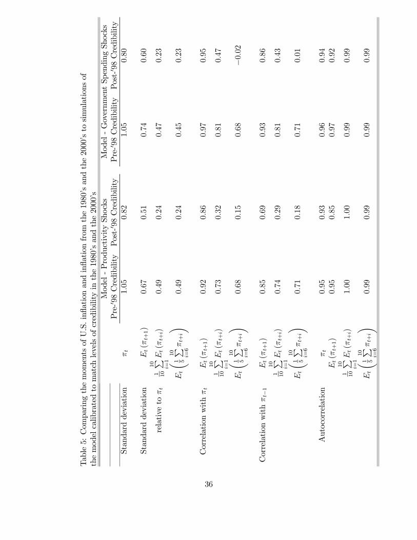
Table5:ComparingthemomentsofU.S.inflationandinflationfrom

the1980’sandthe2000’stosimulationsof

themodelcalibratedtomatchlevelsofcredibilityinthe1980’sandthe2000’s

Model-ProductivityShocks

Model-GovernmentSpendingShocks

Pre-′ 9

8Credibility

Post-′ 9

8Credibility

Pre-′ 9

8Credibility

Post-′ 9

8Credibility

Standarddeviation

πt

1.05

0.82

1.05

0.80

Standarddeviation

Et(π

t+1)

0.67

0.51

0.74

0.60

relativetoπt

1 10

10 ∑ i=1

Et(π

t+i)

0.49

0.24

0.47

0.23

Et

( 1 5

10 ∑ i=6

πt+i)

0.49

0.24

0.45

0.23

Correlationwithπt

Et(π

t+1)

0.92

0.86

0.97

0.95

1 10

10 ∑ i=1

Et(π

t+i)

0.73

0.32

0.81

0.47

Et

( 1 5

10 ∑ i=6

πt+i)

0.68

0.15

0.68

−0.

02

Correlationwithπt−

1Et(π

t+1)

0.85

0.69

0.93

0.86

1 10

10 ∑ i=1

Et(π

t+i)

0.74

0.29

0.81

0.43

Et

( 1 5

10 ∑ i=6

πt+i)

0.71

0.18

0.71

0.01

Autocorrelation

πt

0.95

0.93

0.96

0.94

Et(π

t+1)

0.95

0.85

0.97

0.92

1 10

10 ∑ i=1

Et(π

t+i)

1.00

1.00

0.99

0.99

Et

( 1 5

10 ∑ i=6

πt+i)

0.99

0.99

0.99

0.99

36

1984 1988 1992 1996 2000 2004 2008­5

­4

­3

­2

­1

0

1

2

3

4Inflation

1984 1988 1992 1996 2000 2004 2008­4

­3

­2

­1

0

1

2

31­year­ahead inflation expectations

1984 1988 1992 1996 2000 2004 2008­2

­1

0

1

2

310­year­ahead expectations

1984 1988 1992 1996 2000 2004 2008­1.5

­1

­0.5

0

0.5

1

1.5

2

2.55­year­5­year forward expectations

Figure 1: Headline inflation and measures of inflation expectations in theUnited States from 1984 to 2011.

37

1957 1961 1965 1969 1973 1977 1981 1985 1989 1993 1997 2001 2005 20090

0.01

0.02

0.03

0.04

0.05

0.06

0.07

0.08

Figure 2: Estimated value of the inflation expectations anchoring parameterφ

38

1984 1988 1992 1996 2000 2004 2008­5

­4

­3

­2

­1

0

1

2

3

4Inflation

1984 1988 1992 1996 2000 2004 2008­12

­10

­8

­6

­4

­2

0

2

4

61­year­ahead inflation expectations

1984 1988 1992 1996 2000 2004 2008­4

­3

­2

­1

0

1

2

310­year­ahead expectations

1984 1988 1992 1996 2000 2004 2008­2

­1.5

­1

­0.5

0

0.5

1

1.5

2

2.55­year­5­year forward expectations

Figure 3: U.S. inflation and inflation expectations from 1984 to 2011. Thesolid line is the data, the dashed line is from simulations of the New Keynesianmodel with full price and wage indexation, the line with stars is from the NewKeynesian model with limited central bank credibility.

39