reactive power and voltage control - ieee …sites.ieee.org/fw-pes/files/2013/01/vq_ftworth.pdf ·...
TRANSCRIPT

REACTIVE POWER AND VOLTAGE REACTIVE POWER AND VOLTAGE CONTROL
Salvador Acha Daza, Ph. D.
IEEE Distinguished Power Lecturer
June 2014
Guide
1 MODELINGAssumptions and V, I, P, QTransformers, Transmission Lines, GeneratorsSVC’s (static VAR compensators)
2 BASICS ABOUT VOLTAGE CONTROLQ-V relationReactive power flow and incremental modelDecupled Load-FlowTap’s control and generalized controlTap’s control and generalized control
3 SENSITIVITY Q-V AND COORDINATED CONTROLSensitivity coefficientsApplication and coordinated controlQ-V CongestionRadial networks
4 VOLTAGE COLLAPSEAngle stabilityVoltage collapse
2

Modeling
3

Single phase, steady state: Voltage, Current
• AC voltage and current, f = 60 Hz• rms values: 120 V, 50 A• If current lags voltage by 30o
+
V
-
I
Loadconvention
150
v(t)
4
V
I
f
Phasor plane0 0.002 0.004 0.006 0.008 0.01 0.012 0.014 0.016
-150
-100
-50
0
50
100
time, sec
volta
ge V
, cu
rren
t A
i(t)
v(t)

Complex power S, P and Q
VAjS
jQPIVS
oo 000,31.196,5)3050()0120( *
*
Qf
S
IP
Q
5
P
Qf
Power plane
• cos f is the power factor• The case shows a “lagging power factor”
+
V
-
Loadconvention
R
jwL
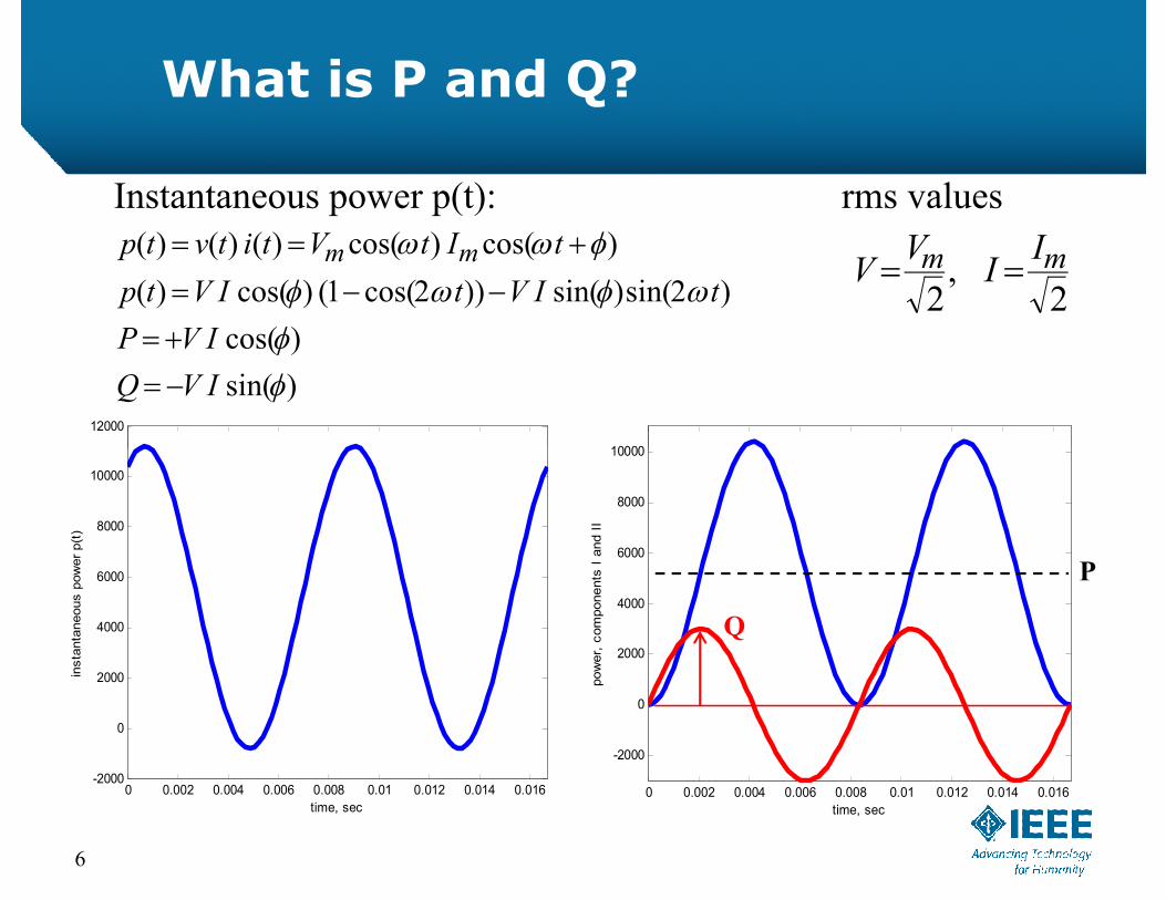
What is P and Q?
Instantaneous power p(t):
)sin(
)cos(
)2sin()sin())2cos(1()cos()(
)cos()cos()()()(
IVQ
IVP
tIVtIVtp
tItVtitvtp mm
2,
2mm I
IV
V
rms values
12000
10000
6
0 0.002 0.004 0.006 0.008 0.01 0.012 0.014 0.016-2000
0
2000
4000
6000
8000
10000
time, sec
insta
nta
neous p
ow
er
p(t
)
P
0 0.002 0.004 0.006 0.008 0.01 0.012 0.014 0.016
-2000
0
2000
4000
6000
8000
10000
time, sec
pow
er,
com
ponents
I a
nd I
I
Q

Voltage and current, steady state
)()( DD
s
XxjRr
VI
Positive sequencexjr
DD XjR sVI
Assuming load and voltage as a fixed value (no use of load flow), ZLine= 0.05 + j0.5 W
Power factor effect on voltage, angle and losses
7
Power factor effect on voltage, angle and lossesNominal load voltage and current (rms values)
120.00 50.00
Voltage source angle PS QS PL QL pf(load) Losses %136.20 8.61 5321.15 4250.00 5196.15 3000.00 -0.87 2.35131.01 10.33 5920.55 2802.91 5795.55 1552.91 -0.97 2.11125.02 11.53 6125.00 1250.00 6000.00 0.00 +1.00 2.04118.57 12.07 5920.55 -302.91 5795.55 -1552.91 +0.97 2.11112.03 11.80 5321.15 -1750.00 5196.15 -3000.00 +0.87 2.35

Transformer Model
For an ideal transformer with complex relation
8
tV
V
k
k 1
'~
~
** ''~~
kmkkmk iViV
t
V
V
i
i
k
k
km
km~'
~
' *
*
Complex, real and reactive power, from k to m:
**** ~'
~~'
~~kmmkkkmkkmkkm yVVtVitViVs
mkkmmkmkkmmkkmkkm btVVgtVVgtVp sincos22
mkkmmkmkkmmkkmkkm btVVgtVVbtVq cossin22

Transmission line model
A symmetric arrangement for a balanced transmission line, positive sequence values, using p equivalent
.
9
kjkk eVV ~
mjmm eVV ~
kmkmkm jbgy
2/2/
2/1
shC
sh jBjX
y
Complex power flow from k to m
mkkm
*, )(
~shkkmkkm iiVs
kmkmmkkmkmmkkmkkm bVVgVVgVp sincos2
kmkmmkkmkmmkshkmkkm bVVgVVBbVq cossin)( 2/2

Simple synchronous machine model
Single phase model, synchronous machine no saliency:
.
asIXjVE
I
VEjX
Equivalent circuit for synchronous machine
Synchronous machine
+E-
Ia +V-
Zs = Ra + jXs
10
IajXs Synchronous machine connected to an infinite bus
Ia
V
E
Zs Iad
IaV
E
Zs Iad
Ia
V
E
Zs Iadq
Load with lagging power factor
Load with unity pf Load with leading pf

SVC characteristics.
Q-V relation
-V
Vm QB = Bmin
B = Bmax
V
1.0
11
+Vo
TCR
capacitiveinductive
B = Bmax
Q-0.2 0 +0.2
TSC (Thyristor Switched Capacitor)TCR (Thyristor Controlled Reactors)

Basics about Voltage Control
12
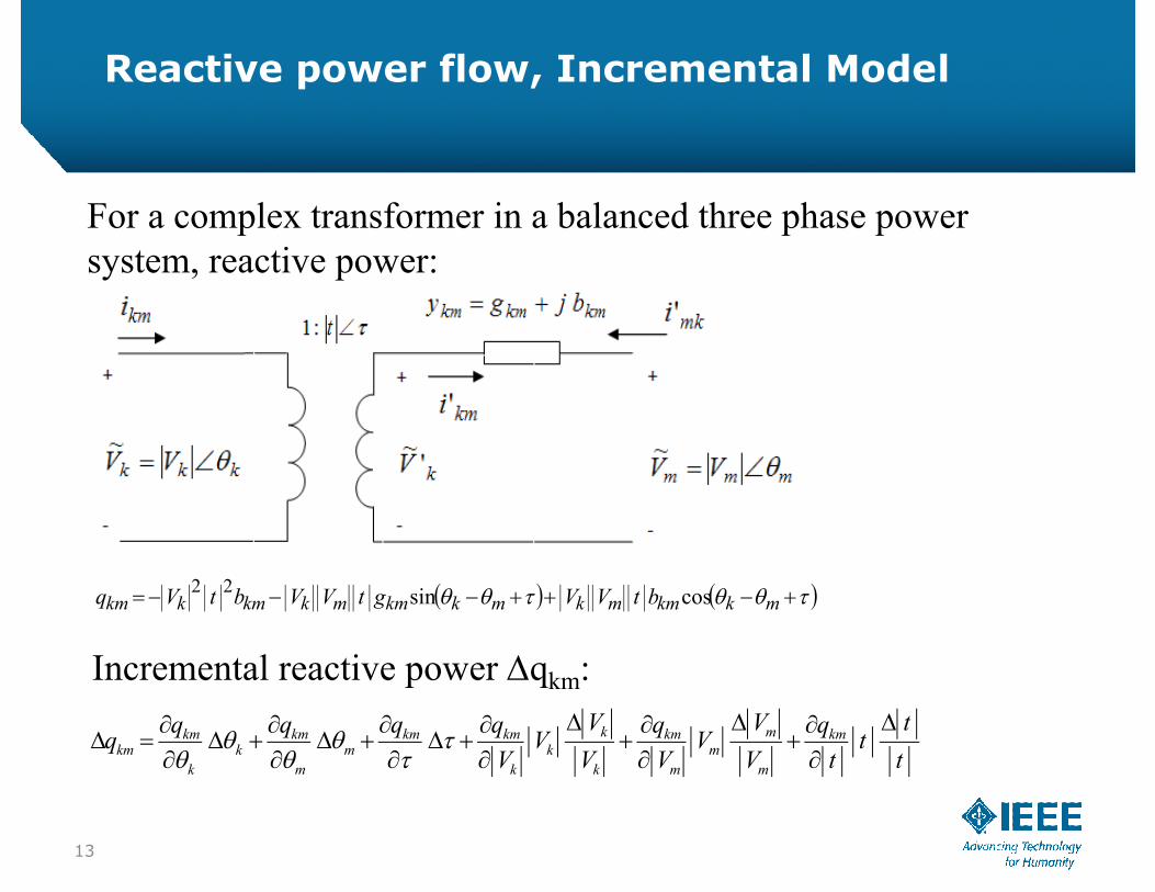
Reactive power flow, Incremental Model
For a complex transformer in a balanced three phase power system, reactive power:
13
mkkmmkmkkmmkkmkkm btVVgtVVbtVq cossin22
Incremental reactive power Dqkm:
t
tt
t
q
V
VV
V
q
V
VV
V
qqqqq km
m
mm
m
km
k
kk
k
kmkmm
m
kmk
k
kmkm

Approximations
Reasonable assumptions will simplify the incremental reactive power flow, like:
mkkmkk
km bVq
mkkmkm
km bVq
mkkmkkm bV
q0.1)cos(
mkmk )sin(
kmkm bg
14
mkkmk bV
kmkk
km bVV
q
kmkm
km bVV
q
kmkkm bVt
q
Substitution into the incremental form:
tVVV
qx mk
k
kmkm
0.1)cos( mk

Ohm’s law and equivalent circuit
Ohm’s circuit to study the incremental reactive power flow in a complex tap transformer:
tVVV
qx mk
k
kmkm
15
B. Stott, O. Alsac, Fast Decoupled Load Flow, IEEE Trans. On Power Apparatus and Systems, Vol. PAS-93, May-June, 1974.

Equivalent circuit for Dq in a transmission line
A similar procedure will give us an incremental circuit equivalent for a transmission line. The right hand side comes from the line charging susceptance.
kkmmkk
kmkm VBshxVV
V
qx
2/2)(
+
DVk
-
+
DVm
-
+ - + -
xkmDqkm/Vk
16
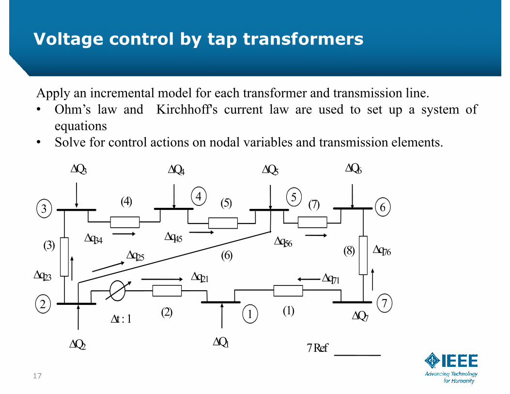
Apply an incremental model for each transformer and transmission line.• Ohm’s law and Kirchhoff's current law are used to set up a system of
equations• Solve for control actions on nodal variables and transmission elements.
Voltage control by tap transformers
Q3 Q4 Q5 Q6
54(4) (5)
17
7 RefQ1Q2
t : 17
1
654
3
2
q71q21q23
q34 q45 q56 q76q25
(1)(2)
(3)
(4) (5)
(6)
(7)
(8)
Q7

7 RefQ1Q2
Q3 Q4 Q5 Q6
t : 17
1
654
3
2
q71q21q23
q34 q45 q56 q76q25
(1)(2)
(3)
(4) (5)
(6)
(7)
(8)
Q7
Ohm´s law for every element(1) 0177171 VVqx
(2) tVVqx 122121
(3) 0322323 VVqx
(4) 0433434 VVqx
(5) 0544545 VVqx
(6) 0522525 VVqx
(7) 0655656 VVqx
(8) 0677676 VVqx
Node equations, Kirchoff´s law
node 1 12171 Qqq node 2 2252321 Qqqq node 3 33423 Qqq node 4 44534 Qqq node 5 5564525 Qqqq node 6 67656 Qqq
18

Sensitivity factors
00110000008
1000
0001100000010
100
00001100000015
10
000001000000015
1
31128.0)4(
31128.0)3(
10117.2)2(
10117.2)1(
Second column of the inverse
00000011000000
00000001110000
00000000011000
00000000001100
00000000100110
00000000000011
10000010
10000000
11000005
1000000
0100100020
100000
01100000016
10000
8
21012.06
63035.05
64981.04
68872.03
71984.02
14008.01
10117.2)8(
10117.2)7(
78988.1)6(
31128.0)5(
31128.0)4(
19

SENSITIVITY Q-V AND COORDINATED CONTROLCOORDINATED CONTROL
20
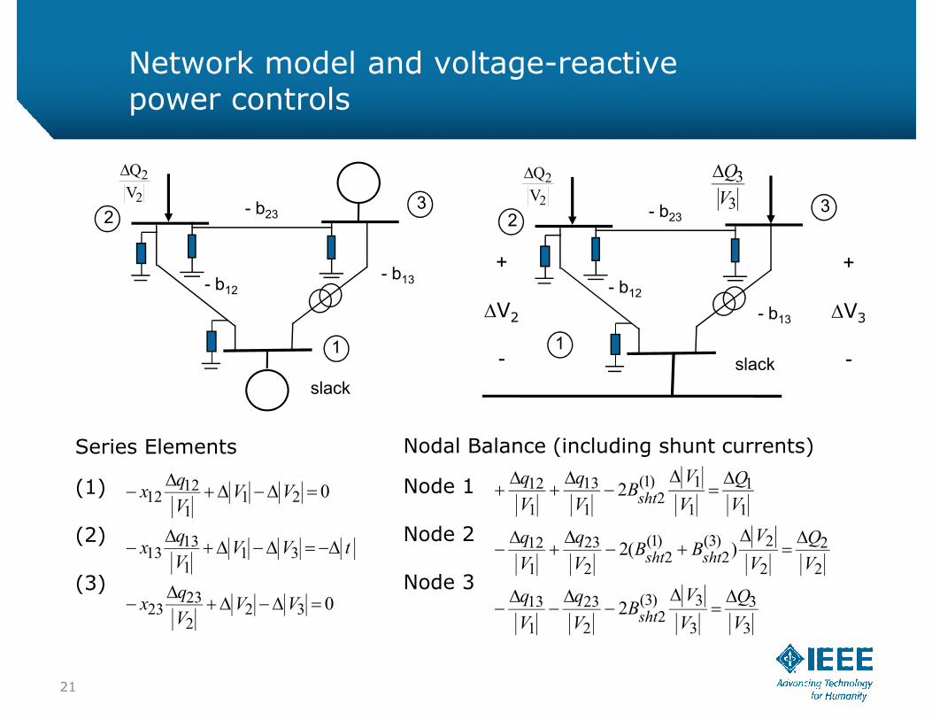
Network model and voltage-reactive power controls
1
- b2323
- b12
2
2VQ
- b13+
DV2
-1
- b2323
slack
- b12
2
2VQ
- b13
+
DV3
-
3
3V
Q
0
0
322
2323
311
1313
211
1212
VVV
qx
tVVV
qx
VVV
qx
Series Elements
(1)
(2)
(3)
slack
Nodal Balance (including shunt currents)
Node 1
Node 2
Node 3
3
3
3
3)3(2
2
23
1
13
2
2
2
2)3(2
)1(2
2
23
1
12
1
1
1
1)1(2
1
13
1
12
2
)(2
2
V
Q
V
VB
V
q
V
q
V
Q
V
VBB
V
q
V
q
V
Q
V
VB
V
q
V
q
sht
shtsht
sht
21
- slack -
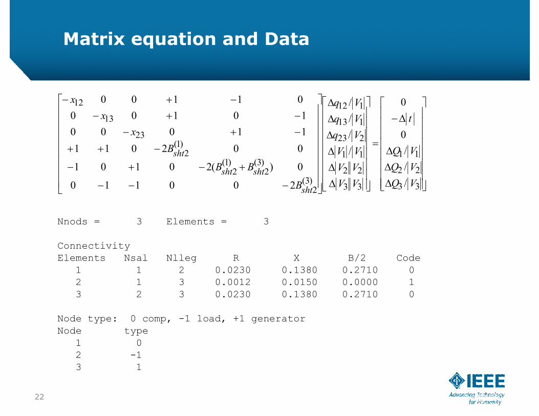
Matrix equation and Data
33
22
11
33
22
11
223
113
112
)3(2
)3(2
)1(2
)1(2
23
13
12
/
/
/
0
0
/
/
/
/
200110
0)(20101
002011
11000
10100
01100
VQ
VQ
VQ
t
VV
VV
VV
Vq
Vq
Vq
B
BB
B
x
x
x
sht
shtsht
sht
Nnods = 3 Elements = 3
ConnectivityElements Nsal Nlleg R X B/2 Code
1 1 2 0.0230 0.1380 0.2710 02 1 3 0.0012 0.0150 0.0000 13 2 3 0.0230 0.1380 0.2710 0
Node type: 0 comp, -1 load, +1 generatorNode type
1 02 -13 1
22
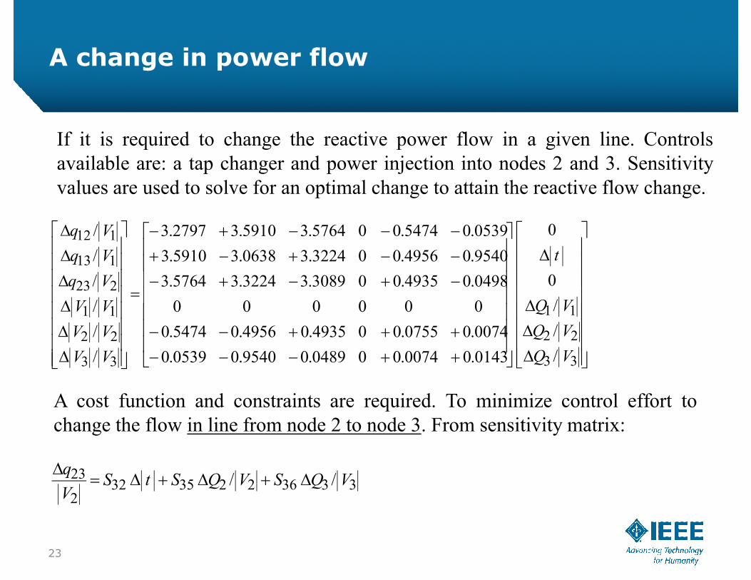
If it is required to change the reactive power flow in a given line. Controlsavailable are: a tap changer and power injection into nodes 2 and 3. Sensitivityvalues are used to solve for an optimal change to attain the reactive flow change.
223
113
112
0
0
0498.04935.003089.33224.35764.3
9540.04956.003224.30638.35910.3
0539.05474.005764.35910.32797.3
/
/
/
t
Vq
Vq
Vq
A change in power flow
A cost function and constraints are required. To minimize control effort tochange the flow in line from node 2 to node 3. From sensitivity matrix:
33
22
11
33
22
11
223
/
/
/
0
0143.00074.000489.09540.00539.0
0074.00755.004935.04956.05474.0
000000
0498.04935.003089.33224.35764.3
/
/
/
/
VQ
VQ
VQ
VV
VV
VV
Vq
33362235322
23 // VQSVQStSV
q
23

Lagrangian and its gradient:
0///.. 3336223532223 VQSVQStSVqas
)()()()(),,(3
336
2
23532
2
232
3
33
2
2
22
21
3
3
2
2V
QS
V
QStS
V
q
V
Qk
V
Qktk
V
Q
V
Qt
2333
2222
21 )/()/()(min VQkVQktk
Cost function and constraints
Gradient must be zero for an optimal solution. We find a set of equationsto be solved for the control actions required.
0
0
0
0
///
/2
/2
2
.
/
/
3336223532223
36333
35222
321
33
22
VQSVQStSVq
SVQk
SVQk
Stk
VQ
VQ
t
24

This case requires to solve a system of linear equations
The change in controls to reduce the reactive power flow q23 in 0.2:
223
33
22
363532
363
352
321
/
0
0
0
/
/
0
200
020
002
Vq
VQ
VQ
t
SSS
Sk
Sk
Sk
The change in controls to reduce the reactive power flow q23 in 0.2:
Smin =2.0000 0 0 -3.3224
0 2.0000 0 -0.49350 0 2.0000 0.0498
-3.3224 -0.4935 0.0498 0
Dy =-0.0589-0.00870.0009-0.0354
ans = -0.2000
0354.0
0009.0
0087.0
0589.0
/
/
33
22
VQ
VQ
t The coordinated changes work to modify the required value, but control limits must be included (i. e. maximum/minimum setting must be observed).
25

Previous solution used k’s as unit values.
Different weight or importance in a control action can be handled through the k values. A change to reduce (or make larger) the control action of injected reactive power is shown by values k2 = 0.1 and k3 = 0.1
Dy =-0.0492-0.07310.0074-0.0296
ans = -0.2000
0296.0
0074.0
0731.0
0492.0
/
/
33
22
VQ
VQ
t
26

A real network might have a structure as shown, in which nodes andtransmission elements show a radial structure; considered “longitudinal”; it isnot a very robust network.
This type of network is very interesting to study control actions and magnitudeof their influence.
Weak and Radial type networks
10 114 10 114
27
104
2 3 9
15 12 15
6
7
8
13
14
104
2 3 9
15 12 15
6
7
8
13
14
15 nodes, 15 elements longitudinal network
(1)(2)
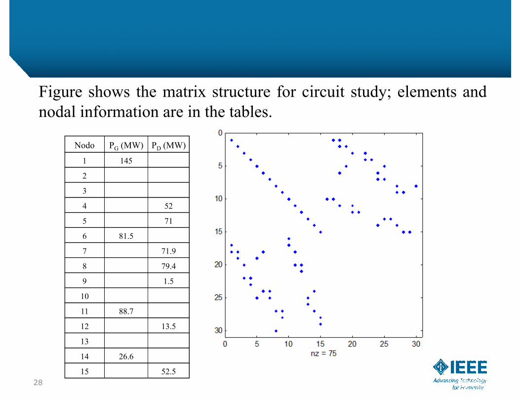
Figure shows the matrix structure for circuit study; elements andnodal information are in the tables.
Nodo PG (MW) PD (MW)
1 145
2
3
4 52
5 71
6 81.5
7 71.9
8 79.4
9 1.5
10
11 88.7
12 13.5
13
14 26.6
15 52.528

15 node system and elements, connectivity and reactance values.
Elemento Nodo Salida - Nodo Llegada x (pu)
(1) 2 - 3 0.1189
(2) 3 - 4 0.0568
(3) 5 - 7 0.0807
(4) 7 - 8 0.0451(4) 7 - 8 0.0451
(5) 4 - 10 0.1316
(6) 3 - 9 0.1458
(7) 10 - 9 0.0449
(8) 12 - 15 0.1699
(9) 12 - 13 0.0849
(10) 1 - 2 0.09303
(11) 3 – 5 0.1885
(12) 6 – 5 0.1330
(13) 11 – 10 0.0930
(14) 9 – 12 0.1885
(15) 14 - 13 0.1331
transformers
lines
29

S =Columns 1 through 8 -3.1237 -0.9899 0 0 -0.9899 -1.0824 0.6391 0-0.9899 -3.4485 0 0 -3.4485 1.8060 -1.9376 -0.0000
0 0 0 0 0 0 0 00 0 0 0 0 0 0 0
-0.9899 -3.4485 0 0 -3.4485 1.8060 -1.9376 -0.0000-1.0824 1.8060 0 0 1.8060 -3.6018 2.9980 00.6391 -1.9376 0 0 -1.9376 2.9980 -4.4065 0
0 0 0 0 0 0 0 0-0.4433 -0.1316 0 0 -0.1316 -0.6039 -1.4085 0-3.1237 -0.9899 0 0 -0.9899 -1.0824 0.6391 0-1.0513 0.6526 0 0 0.6526 0.7135 -0.4213 0.00001.0513 -0.6526 0 0 -0.6526 -0.7135 0.4213 -0.00001.0513 -0.6526 0 0 -0.6526 -0.7135 0.4213 -0.00001.6290 1.5109 0 0 1.5109 1.1920 -2.4688 0-0.4433 -0.1316 0 0 -0.1316 -0.6039 -1.4085 00.4433 0.1316 0 0 0.1316 0.6039 1.4085 0
0.0000 0.0000 0 0 0.0000 0.0000 -0.0000 -0.00000.2906 0.0921 0 0 0.0921 0.1007 -0.0595 0-0.3380 0.2098 0 0 0.2098 0.2294 -0.1354 0-0.2818 -0.5943 0 0 0.4057 0.1268 -0.0254 -0.0000-0.1398 0.0868 0 0 0.0868 0.0949 -0.0560 0.0000-0.0000 0.0000 0 0 0.0000 0.0000 -0.0000 0-0.1398 0.0868 -1.0000 0 0.0868 0.0949 -0.0560 0.0000-0.1398 0.0868 -1.0000 -1.0000 0.0868 0.0949 -0.0560 0.0000-0.1802 -0.0535 0 0 -0.0535 -0.2455 -0.5725 0-0.1515 -0.1405 0 0 -0.1405 -0.1109 0.2296 0-0.0000 -0.0000 0 0 -0.0000 -0.0000 0.0000 0-0.0966 -0.0287 0 0 -0.0287 -0.1316 -0.3070 0-0.0590 -0.0175 0 0 -0.0175 -0.0804 -0.1875 0-0.0000 -0.0000 0 0 -0.0000 -0.0000 -0.0000 -0.0000-0.0966 -0.0287 0 0 -0.0287 -0.1316 -0.3070 -1.0000

Q-V RELATION AND VOLTAGE SUPPORTSUPPORT
31

Voltage and current, steady state
)()( DD
s
XxjRr
VI
Positive sequencexjr
DD XjR sVI
Assuming load and voltage as a fixed value (no use of load flow), ZLine= 0.05 + j0.5 W
Power factor effect on voltage, angle and losses
32
Power factor effect on voltage, angle and lossesLoad voltage and current, rms values
120.00 50.00
Voltage source angle PS QS PL QL pf(load) Efficiency136.20 8.61 5321.15 4250.00 5196.15 3000.00 -0.87 2.35131.01 10.33 5920.55 2802.91 5795.55 1552.91 -0.97 2.11125.02 11.53 6125.00 1250.00 6000.00 0.00 +1.00 2.04118.57 12.07 5920.55 -302.91 5795.55 -1552.91 +0.97 2.11112.03 11.80 5321.15 -1750.00 5196.15 -3000.00 +0.87 2.35

PV curve and load characteristics
0.4
0.6
0.8
1
volta
ge V
m, p
u
P-V curve, DC circuit
33
0 0.5 1 1.5 2 2.50
0.2
power PL, pu
System’s PV curve and for a resistive load, RL = 1.5, 1.1 pu.
