2002

Russian River First Flush Summary Report

by Revital Katznelson Clean Water Team, the Citizen Monitoring Program of the

State Water Resources Control Board

In collaboration with

Richard Fadness Lauren Hocker Robert Klamt

North Coast Regional Water Quality Control Board

June 2003

ACKNOWLEDGEMENTS This report was prepared with a very substantial help and input from the staff of the North Coast Regional Water Quality Control Board (RB1), including data analysis, plotting, and mapping, for which I am deeply grateful. The contribution of RB1 staff to the monitoring efforts through all the phases of preparation, deployment, and lab analysis is also acknowledged with thanks. Many thanks are due to the Russian River Field Crews and Captains who participated in the sampling efforts with devotion, preparedness, and willingness to face the elements. The dedication and hard work of the Organizers, Hubsters, and Lab Manager who tackled all the logistical challenges is highly appreciated, as well as the generosity of the Sotoyome RCD folks who gave us essential sample staging space. Last but not least, I would like to thank the Lab & Data Coordinator, the Lab Volunteers, and the Data Management Crew for the best data capture I could hope for!

RK 4/4/03

DISCLAIMER The data contained in this report has been collected by citizen volunteers or generated from samples collected by volunteers. The results that are reported have been measured and documented in good faith and to the best of the volunteers’ abilities. Nothing in this report should be used to the detriment of the volunteer/property owner, their property, or the program in which they are involved. It should also be understood that volunteers collect information voluntarily and there are limitations on the use of their data. Data can serve as a preliminary source of information only to be followed up, when necessary, with more formal types of monitoring.

Table of Contents

Page1.0 Introduction

1

2.0 Study plan and logistics

3

3.0 Results and interpretation

11

4.0 Data quality overview

24

5.0 Summary and recommendations

26

6.0 Glossary

27

APPENDIX A: RRFF Stations and Participants APPENDIX B: QA/QC Report (available upon request, with electronic Project File) APPENDIX C: Standard Operating Procedures (available upon request) APPENDIX D: Result Graphics (by NCRWQCB, available upon request)

1

1.0 Introduction Volunteer monitoring has become an integral part of the effort to assess the health of our nation's waters. It promotes stewardship of local waters, and provides an educational tool to teach citizens about the importance of environmental quality. In addition, government agencies have found that properly run volunteer programs can provide high quality information to supplement their own monitoring programs. On November 7th 2002, over 100 citizen monitors conducted field measurements and collected water samples at multiple locations within the Russian River (RR) Watershed during the first runoff event of the rainy season. It was the local watershed groups that made it happen, led by the dedicated Volunteer Coordinator who worked with members of the Russian River Watershed Council, Resource Conservation Districts, volunteers from Cities and other local agencies, and many citizen groups. The idea sprang up a few months earlier when the Scientific Coordinator, a Clean Water Team member and a First-Flush ‘pro’, talked with folks at the Regional Water Quality Control Board and heard a wish to collect First Flush (FF) samples in this watershed. The Russian River First Flush (RRFF) monitoring was intended to characterize the runoff in different parts of the watershed and identify sources of potential pollutants (Please note that stormwater ‘constituents’ such as ammonia, metals, or sediments are not considered ‘pollutants’ if it has not been shown that they cause a problem, as in “innocent until proven guilty”). In other words, the objective of sampling at multiple tributaries was to gather information from the various drainages and develop some perspective on the occurrences of the major constituents. Information gleaned from this characterization effort can help citizens, local agencies, and regulators prioritize future management options. Although limited in geographical coverage, the event provided an opportunity to pose some specific questions, such as: · Where in the RR watershed does the first rain event of the season yield runoff? · What are the highest concentrations of stormwater constituents in urban areas in the RR watershed? · Are there sources of diazinon in the RR watershed? · Are the E.coli counts during First Flush in the RR watershed at the same order of magnitude as the First Flush counts in other watersheds? A unique partnership between citizen groups, academia, and public agencies – local, State, and Federal - was established to accomplish data collection. The citizen coordinators in charge of field activities conducted an outreach campaign, recruited more than 100 citizens, arranged training sessions and transfers of equipment & samples, and constructed a phone tree to spread the rain alerts among participating field crews. Citizens also participated in lab analyses and data entry, working shoulder to shoulder with agency staff. The Regional Citizen Monitoring Coordinator of the Clean Water Team (the Citizen Monitoring Program of the State Water Resources Control Board) provided technical support, training, in-house nutrient analysis guidance, laboratory liaison, and data quality management tools/guidance. Folks from Sonoma State University, Sotoyome Resource Conservation District, and UC Cooperative Extension

2

helped with hydrological information, station selection, and weather watch. North Coast Regional Water Quality Control Board (RB1) staff and interns provided technical input, in-house lab space, in-house lab management and analytical support, and budget for metal analysis. EPA Region IX staff lent monitoring equipment to the effort and provided lab analyses of bacteria and pesticides, and the City of Santa Rosa contributed analytical budget for pesticide confirmation testing. This unique combination of community outreach and technical support contributed to the success of the event in its dual achievements: water pollution awareness, and good data. In other words, word got out into the community regarding how our daily activities may be sources of constituents, and the technical effort yielded reliable data of known quality.

3

2.0 Study plan and logistics In semi-arid, Mediterranean climate zones where summers are dry and rain falls only in winter, the term ‘First Flush’ is often used to describe the stormwater runoff that flows into creeks after the first rain of the winter has washed the landscape. Research has shown that this First Flush runoff is often laced with constituents that have accumulated over the land during summer, and thus represents ‘the worst case scenario’ in terms of storm water pollution in many cases. RRFF study plan was constructed to capture these ‘worst case scenario’ conditions in order to learn about the severity of pollution problems in the watershed. 2.1 Study Intent, Sampling Design, and Power: Theory and practice. A Monitoring Plan includes elements that communicate the “why, what, where, when, how, and who” of the study. The term ‘study intent’ as used here refers to the ‘why monitor’ part of the plan, and basically implies “what do we want to know?”. RRFF study plan was geared towards two major questions: Are there hot spots (i.e., the intent is characterization), and where are they (i.e., the intent is source ID). The term ‘sampling design’ is used here in the narrow sense, meaning the approach used to deliberately select timing and locations for sampling (Please note that here the word ‘sampling’ includes both field measurement and sample collection). We chose the ‘deterministic’, i.e., knowledge-based approach, rather than the ‘probabilistic’ i.e., random approach. This ‘directed’ sampling design principle led us to build the study logistics based on what we already know about FF, i.e., in a way that will enable sampling during the first two hours of runoff. It also led us to choose locations based on our knowledge of what each tributary represents. Application of this ‘directed’ approach yielded a long list of sampling locations that provides a good representation of all the land uses and activities in the Russian River Watershed. Monitoring these Stations should generate a dataset that will answer our questions, that was the theory and it was certainly correct. However, in practice we had to cut down the list based on a number of logistical considerations, the major one being time limitation. For this event we could only accommodate sample collection within the first 10 hours of the rain event, because all samples had to be shipped on one batch and be analyzed within a short holding time. The list of potential sampling locations was therefore shrunk to contain sites that had high probability of generating runoff soon after the rain starts. These sites were mostly in urban, highly paved and roofed landscapes, and the study question was amended to specify this. Other constraints, stemming from recruitment realities, were related to the number of available teams and to their whereabouts; this narrowed the list even more. Health and safety constraints, legal constraints, and other criteria were also instrumental in determining locations. On top of all this, please recall that First Flush sampling efforts, by their very nature, always include a combination of established sampling design principles and some unpredicted, opportunistic, or responsive element (for example, catch runoff samples

4

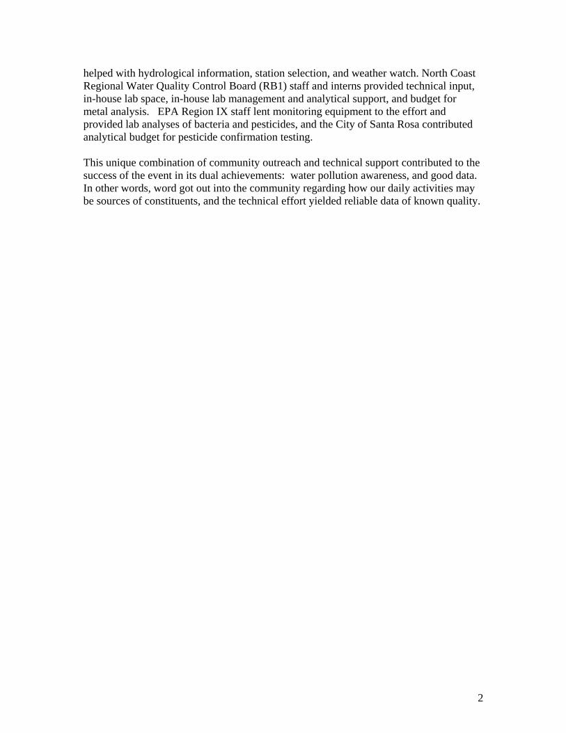
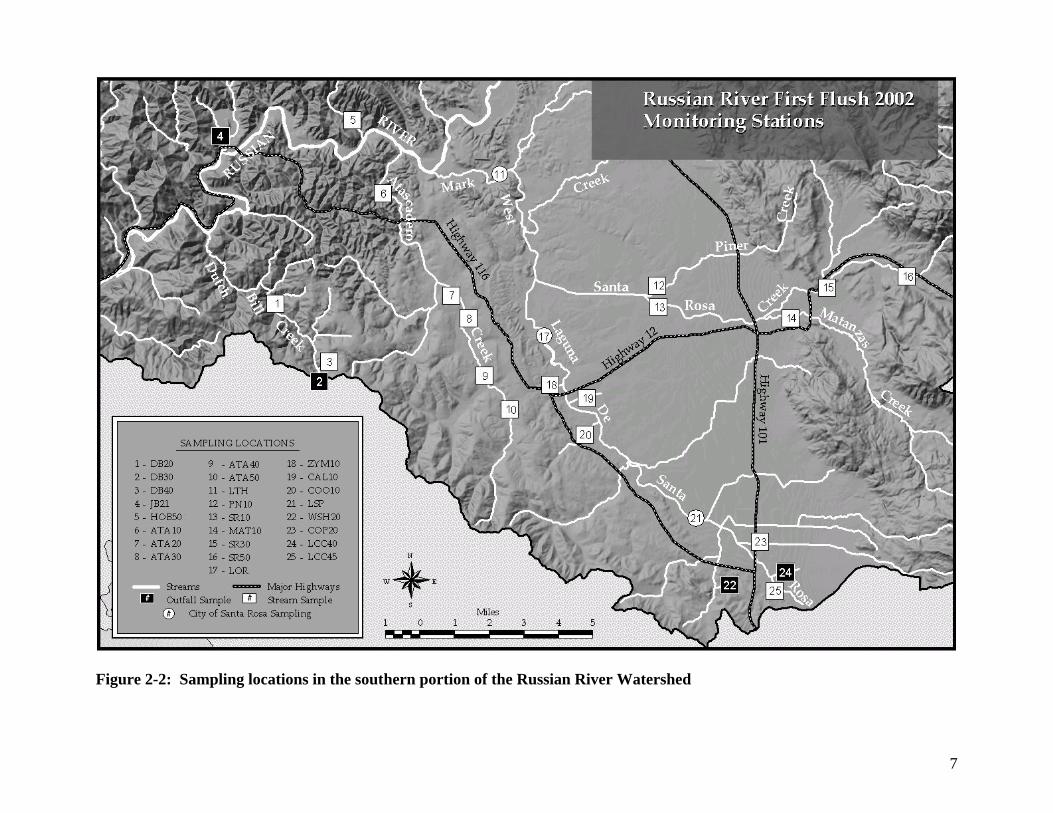
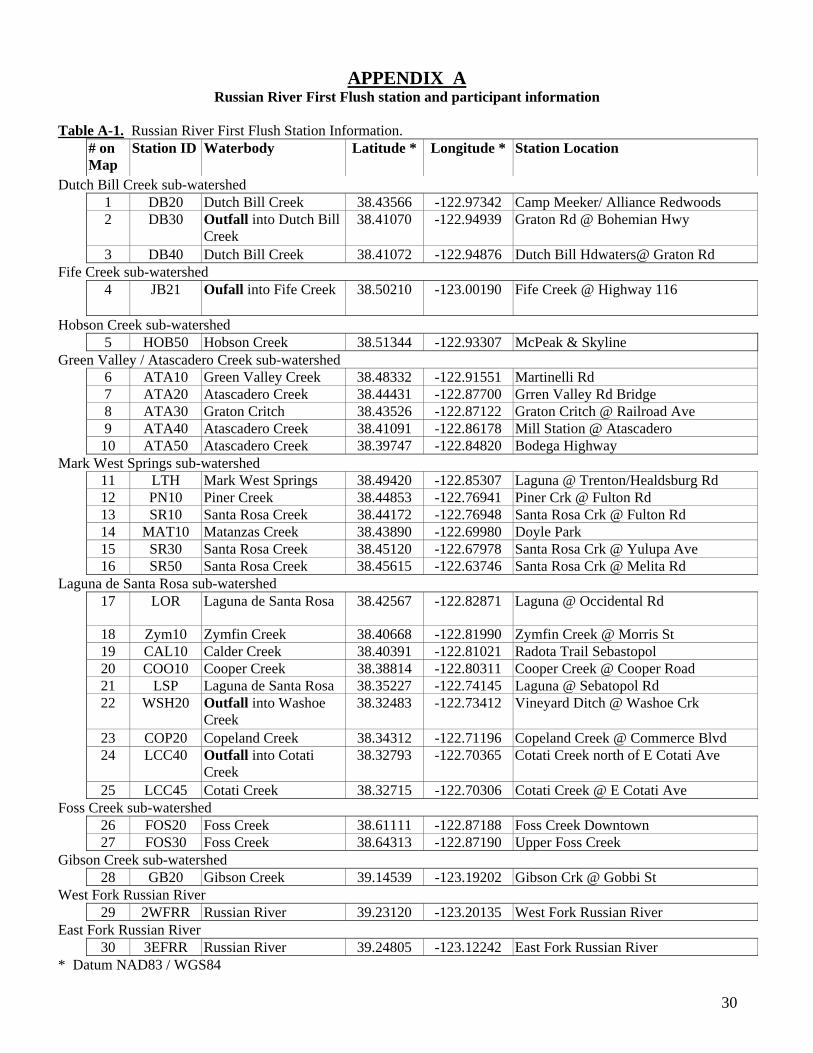
where runoff happens). Thus, the spatial sampling design was based on deliberate decisions where possible, but in some cases the availability of crews – and runoff! -determined where samples were actually collected. The temporal sampling design was based on decisions triggered by actual field conditions meeting “Runoff Criteria” (see below) and was successful in targeting the first hours of runoff. The power of a dataset depends on the number of samples collected and on what each sample represents. By collecting three consecutive runoff samples (i.e. a sample triad) at each Station, the RRFF dataset provides confirmation that detection of high constituent concentrations was not an artifact or a case of a transient spike. Sample triads also provide information on the extent of change over time in a given Station during the sampling period (which was not even the entire event in our case). 2.2 Station Locations As mentioned above, a list of sampling Stations at locations that are safe, accessible, legal, and useful to the data users was prepared. This list included locations offered by citizens living in the watershed. A subset of Stations that have a high likelihood of having runoff during the first storm of the season were selected from that list. Citizen volunteers were assigned to these Stations where possible. Figures 2-1 and 2-2 show the RRFF Stations on a map of the northern and southern parts of the watershed, respectively. The map includes creek stations (white squares) and outfalls (dark squares) sampled by RRFF volunteers, as well as creek stations visited by Santa Rosa City crews (white circles). The Stations were numbered sequentially, from the mouth upstream. Table A-1 (Appendix A) provides detailed information about each Station. Of the locations visited by volunteers on November 7th 2002, most (21) yielded runoff.

6

Figure 2-1: Sampling locations in the northern portion of the Russian River Watershed

7

Figure 2-2: Sampling locations in the southern portion of the Russian River Watershed

8

2.3 Event Logistics The event was coordinated through an ‘Event Center’ and several ‘Hubs’, each associated with several Teams of field operators. The Hubs served as centers for coordination and transfer of information, alerts, equipment, and samples. Hubsters interacted with the event organizers (Volunteer Coordinator, Scientific Coordinator, and RB1 Lab liaison) on one side and with their Captains (Team Leaders) on the other side to create the needed links. The Sotoyome RCD served as the Event Center (from which all samples were sent to EPA and RB1 labs) and coordinated four Hubs in the southern part of the watershed (Dutch Bill, Santa Rosa, Cotati/Rohnert Park, and Healdsburg). Each of these four Hubs had contact with two or more Teams. In the north, the Ukiah Hub was associated with three Teams that were active in their specific area. [Please note that during preparation for the event some of these Hubs were referred to as ‘sub-hubs’]. Preparation for sampling was performed by the Scientific Coordinator and involved technical liaison with EPA lab, borrowing instruments and gathering pre-cleaned sampling containers from different sources, purchasing and decontaminating sampling devices, preparing Field Data sheets and data quality management tools, and planning. The Scientific Coordinator was also in charge of deciding when to mobilize and of preparing the samples for shipping after the event. 2.4 Training Two training sessions were organized by the Hubsters and taught by the Scientific Coordinator, one in each Hub. Agenda items included (a) an introduction about the importance of FF sampling, what will be done with the samples and how the data will be used; (b) overview of the Project logistics; (c) demonstration of the sampling kit items and how to use them, how to label the samples and record information on the Field Data Sheet; (d) hands-on session; (e) Team and Stations assignment and construction of a phone tree (organizers helped with this task); and (f) distribution of field equipment assemblage to teams and loan documentation (Hubsters helped with this task). Consecutive training sessions were held later, taught by Hubsters who had participated in the initial training. 2.5 Alerts, Mobilization, and Runoff Criteria The Volunteer Coordinator developed a Phone Tree comprised of contact information for each participant to assure that word gets out from the Organizers to the Event Center and through the Hubs to individual Teams. An email list of RRFF participants was also gathered and used to disseminate information. The two RRFF ‘weathermen’ watched weather models since early October, and the information was used to make rain alert decisions at three levels: yellow, orange, and red. Yellow alert meant “we are watching a weather system that may come in within 2-4 days”; Orange alert: “a system with >40 percent chance of bringing >0.2” of rain is forecast within 24 hours”; and Red alert meant “we have mobilized! Go to your Stations” (it also meant we are expecting to collect samples and deliver them to the lab within less than 24 hours).

9

The Phone Tree was activated to spread the Yellow alert on November 3rd . Orange alert was called on November 5th, and when it looked like rain was certain and imminent, Red Alert was called on November 6 and spread through the Phone Tree during the late evening before the rain began. This gave the teams a chance to get ready. Upon Red alert, the volunteers were instructed to wait for the rain, watch for the effect of rain in their area, and mobilize when they see water moving from the street surface to the street gutter (in urban areas) or when they see water ponding on the ground (rural areas). Once they arrived at the Station, they used the following Runoff Criteria to identify stormwater runoff:

• When it rains, any flow from an outfall or in a previously dry creekbed is probably runoff, particularly if the water is murky and has cigarette butts floating in it.

• In creeks that already have base flow, stormwater runoff may be present when one can see (a) significant drop in conductivity, (b) visible increase in murkiness, and/or (c) visible rise in water level (stage).

These conditions were observed in 21 Stations, and were followed by collection of three consecutive samples at roughly 30 minute intervals at each station. In five of the 26 Stations runoff was not observed during the 12 hours of RRFF event, and only one sample, representing base flow, was collected in each of these Stations. 2.6 Data Acquisition, Field Measurements, and Laboratory Analyses The parameter package for RRFF is based on pre-determined design where possible and on availability where not. Given that the effort was run essentially without budget, field measurements were limited to available instruments and analytical work was limited to an in-house laboratory or laboratory services provided to volunteers at no cost. (1) Rainfall was gleaned from precipitation reports of three weather stations in the southern part of the RR watershed. RRFF weatherman obtained these data after the event. The following parameters were measured in the field: (2) Stage – water level - was read from staff or wire gauges (or measured directly where access permitted) at selected time periods during the hours of field activity. Some teams were able to evaluate flow discharge using the float method. (3) Electrical conductivity and (4) pH were measured in the field using pocket conductivity meters and pH strips provided by SWRCB/EPA. (5) Temperature was measured by some of the teams using their own equipment. Water (6) murkiness was observed and recorded frequently during the hours of field activity. Water samples were collected in previously decontaminated sampling devices. On site, the devices were rinsed in creek water three times prior to sample collection. Each sample was transferred into three pre-cleaned or sterile containers, all sharing the same Sample ID. This process was repeated every 30 minutes, yielding three independent

10

samples - packed in a total of nine containers - at each Station. Most Teams measured and recorded conductivity, pH, temperature, and stage while – or immediately after – the sample containers were filled. Some Teams also collected field duplicates or equipment blanks while in the field. All samples were delivered to the Event Center at the Sotoyome RCD in Santa Rosa, logged into the chain of custody forms, and split into two sets of coolers (ice chests); one made ready for the RB1 lab and the other for the EPA lab. The first set of sample coolers (with ‘wet’ ice, see glossary) was delivered to RB1 for in-house analyses. (7) Ammonia and (8) ortho-phosphate concentrations were determined by wet-chemistry with a calibration curve and a spectrophotometer, while (9) nitrate was measured (for selected samples) using field kits. Evaluation of suspended sediments included (10) turbidity (measured with a turbidimeter), and (11) total suspended solids (determined gravimetrically by filtering and weighing of the dry residue). The second set of sample coolers (with ‘blue’ ice) was delivered to the EPA lab in Richmond for analyses by EPA staff. The pesticide (12) diazinon, a widely used insecticide, was measured by the enzyme-linked immunosorbent assay (ELISA) method. Bacterial counts evaluated (13) E. coli and (14) Total Coliform using the enzyme-substrate Colilert reagent in Quantitrays. The ecological significance and the regulatory benchmarks for each parameter are often site-specific and related to a specific beneficial use. In addition, the sources of the different constituents may vary depending on land use, and the severity of impact may depend on ambient conditions. All this information has been provided in numerous documents, and could not be detailed in this report. Some background facts are provided in the Results section where possible. Materials for further reading are available with the Project’s Scientific Coordinator, and the reader is referred to Appendix A, Table A-2, for her contact information. 2.7 Data Quality management All information related to the RRFF efforts has been packaged in the DQM Project File established for the RRFF Project. The Project File is an Excel workbook with multiple spreadsheets that hold all the bits of information that the QA/QC officer and the data user will want to see in order to be able to validate, qualify, and use the Results. It allows for the first and most basic function of a data management system, data documentation, and for streamlined QA/QC review and data validation. The file also communicates information on the sampling intent, monitoring questions, and sampling design. Appendix B of this report provides specific information about how the different qualifiers have been derived and where to find what within the Project File.

11

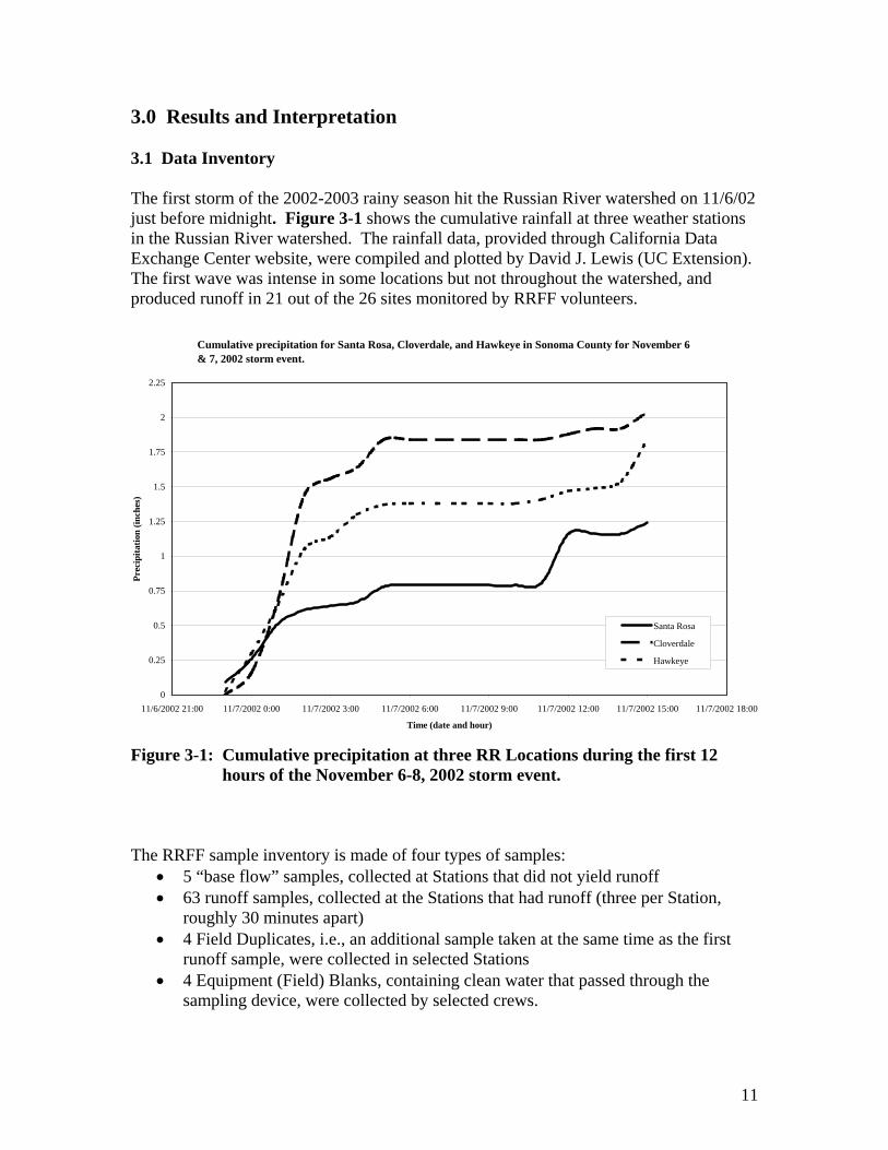
3.0 Results and Interpretation 3.1 Data Inventory The first storm of the 2002-2003 rainy season hit the Russian River watershed on 11/6/02 just before midnight. Figure 3-1 shows the cumulative rainfall at three weather stations in the Russian River watershed. The rainfall data, provided through California Data Exchange Center website, were compiled and plotted by David J. Lewis (UC Extension). The first wave was intense in some locations but not throughout the watershed, and produced runoff in 21 out of the 26 sites monitored by RRFF volunteers.

Figure 3-1: Cumulative precipitation at three RR Locations during the first 12 hours of the November 6-8, 2002 storm event.

The RRFF sample inventory is made of four types of samples:

• 5 “base flow” samples, collected at Stations that did not yield runoff • 63 runoff samples, collected at the Stations that had runoff (three per Station,

roughly 30 minutes apart) • 4 Field Duplicates, i.e., an additional sample taken at the same time as the first

runoff sample, were collected in selected Stations • 4 Equipment (Field) Blanks, containing clean water that passed through the

sampling device, were collected by selected crews.

Cumulative precipitation for Santa Rosa, Cloverdale, and Hawkeye in Sonoma County for November 6 & 7, 2002 storm event.

0

0.25

0.5

0.75

1

1.25

1.5

1.75

2

2.25

11/6/2002 21:00 11/7/2002 0:00 11/7/2002 3:00 11/7/2002 6:00 11/7/2002 9:00 11/7/2002 12:00 11/7/2002 15:00 11/7/2002 18:00

Time (date and hour)

Prec

ipita

tion

(inch

es)

Santa Rosa

Cloverdale

Hawkeye

12

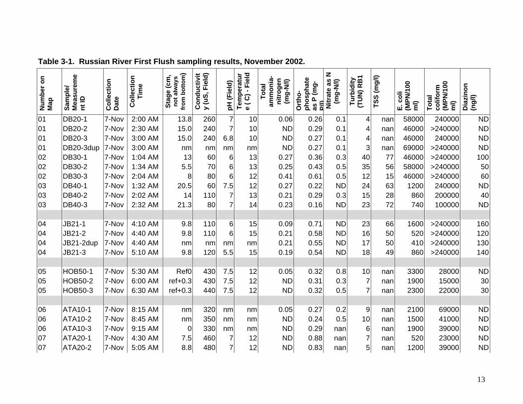
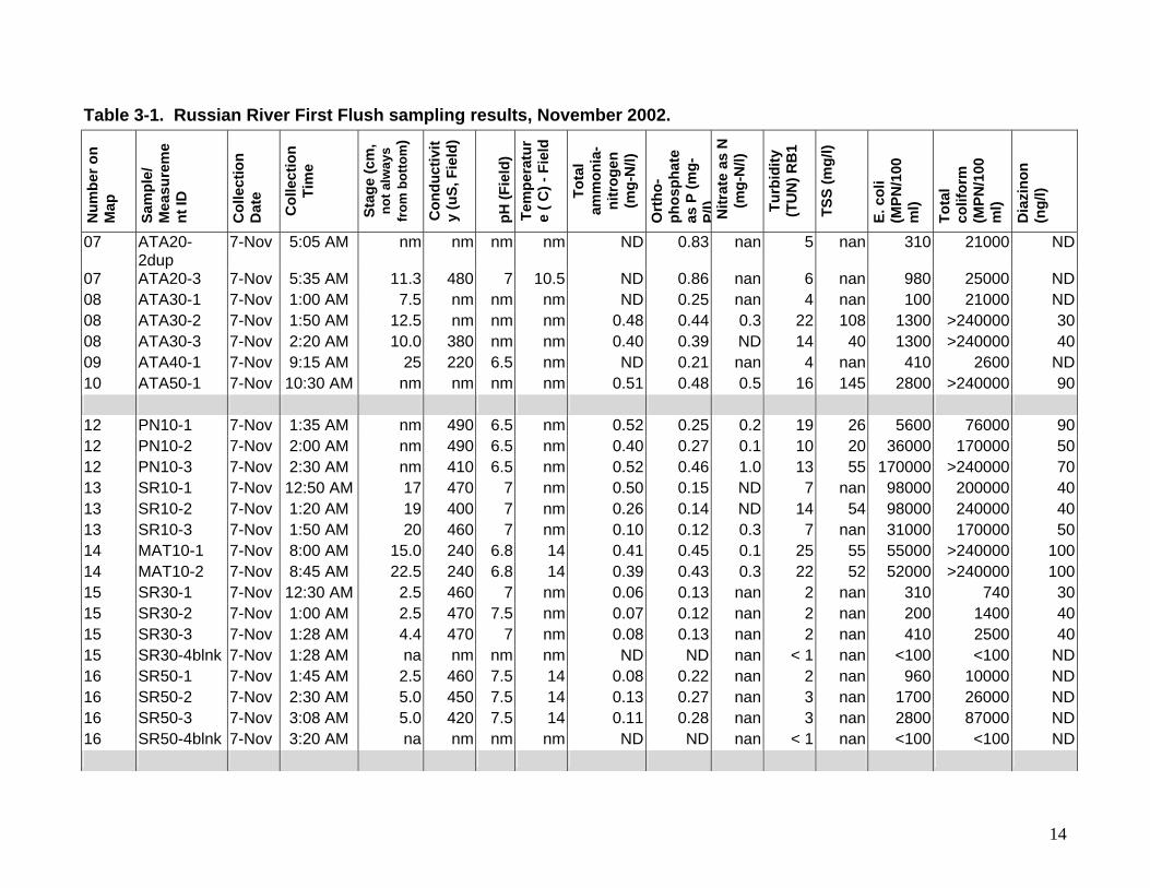
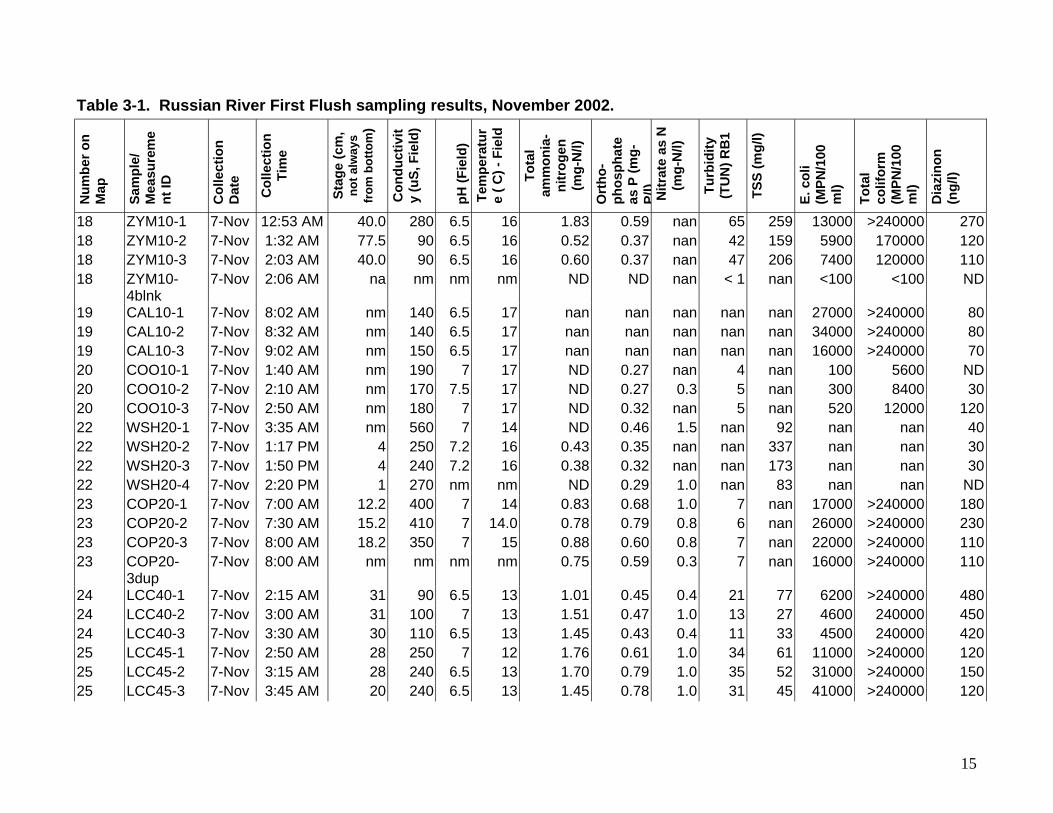
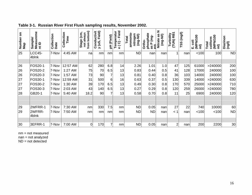
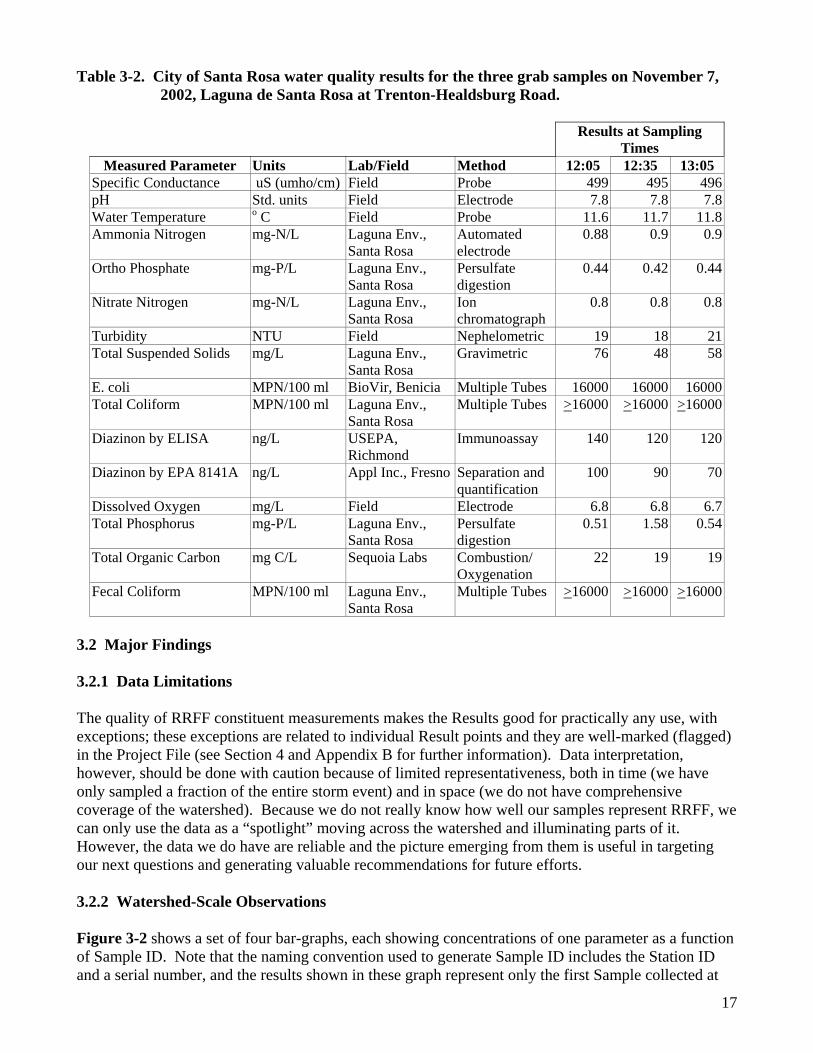
The total of number of samples (including field duplicates and blanks) was 80, and each sample was analyzed for all of the parameters except for a few cases. Table 3-1 shows summary of all results. Stations are listed in the same order as the map numbers sequence, from the mouth up. The “holes” in the table are due to one of several reasons: (a) logistics (e.g., at CAL10 the crew did not have sampling containers for nutrients, turbidity and TSS); (b) volume or material limitations (e.g., samples with low turbidity and small volume did not contain the 2 mg of suspended solids needed for a reliable TSS measurement); or (c) lack of field equipment to measure temperature or pH (which were optional parameters). In the RB1 lab, turbidity was measured first and the results were used to decide which samples need to be filtered for nutrients, which samples have enough particulate matter for TSS, etc. The Result table (Table 3-1) contains all Sample results but also the analytical results for the Field Duplicates and Equipment (Field) Blanks. Field duplicates (marked with “dup” attached to the Sample ID) provide a measure of the reproducibility of our entire sampling and analysis procedure. Equipment Blanks (marked “blnk” attached to the Sample IDs ending with number 4, except WSH20-4) provide proof that our samples were not contaminated. It is obvious that the duplicate Results are very close to each other, and that the Blanks came out very clean. Further discussion about the quality of the data is provided in Section 4 below. The City of Santa Rosa collected grab samples at the Trenton-Healdsburg Road location on November 7, 2002 at 12:05, 12:35, and 1:05 p.m. The results of those samples are presented separately in Table 3-2, below. The only notable changes were a decrease in total suspended solids and a spike in total phosphorus at 12:35 p.m. Additional data, covering the period of noon on November 6 to noon on November 13. 2002 are presented in Appendix D.

13

Table 3-1. Russian River First Flush sampling results, November 2002.

Num

ber o

n M

ap

Sam

ple/

M

easu

rem

ent

ID

Col

lect

ion

Dat

e

Col

lect

ion

Tim

e

Stag

e (c

m,

not a

lway

s fr

om b

otto

m)

Con

duct

ivit

y (u

S, F

ield

)

pH (F

ield

) Te

mpe

ratu

re

( C) -

Fie

ld

Tota

l am

mon

ia-

nitr

ogen

(m

g-N

/l)

Ort

ho-

phos

phat

e as

P (m

g-P/

l) N

itrat

e as

N

(mg-

N/l)

Turb

idity

(T

UN

) RB

1

TSS

(mg/

l)

E. c

oli

(MPN

/100

m

l)

Tota

l co

lifor

m

(MPN

/100

m

l)

Dia

zino

n (n

g/l)

01 DB20-1 7-Nov 2:00 AM 13.8 260 7 10 0.06 0.26 0.1 4 nan 58000 240000 ND 01 DB20-2 7-Nov 2:30 AM 15.0 240 7 10 ND 0.29 0.1 4 nan 46000 >240000 ND 01 DB20-3 7-Nov 3:00 AM 15.0 240 6.8 10 ND 0.27 0.1 4 nan 46000 240000 ND 01 DB20-3dup 7-Nov 3:00 AM nm nm nm nm ND 0.27 0.1 3 nan 69000 >240000 ND 02 DB30-1 7-Nov 1:04 AM 13 60 6 13 0.27 0.36 0.3 40 77 46000 >240000 100 02 DB30-2 7-Nov 1:34 AM 5.5 70 6 13 0.25 0.43 0.5 35 56 58000 >240000 50 02 DB30-3 7-Nov 2:04 AM 8 80 6 12 0.41 0.61 0.5 12 15 46000 >240000 60 03 DB40-1 7-Nov 1:32 AM 20.5 60 7.5 12 0.27 0.22 ND 24 63 1200 240000 ND 03 DB40-2 7-Nov 2:02 AM 14 110 7 13 0.21 0.29 0.3 15 28 860 200000 40 03 DB40-3 7-Nov 2:32 AM 21.3 80 7 14 0.23 0.16 ND 23 72 740 100000 ND 04 JB21-1 7-Nov 4:10 AM 9.8 110 6 15 0.09 0.71 ND 23 66 1600 >240000 160 04 JB21-2 7-Nov 4:40 AM 9.8 110 6 15 0.21 0.58 ND 16 50 520 >240000 120 04 JB21-2dup 7-Nov 4:40 AM nm nm nm nm 0.21 0.55 ND 17 50 410 >240000 130 04 JB21-3 7-Nov 5:10 AM 9.8 120 5.5 15 0.19 0.54 ND 18 49 860 >240000 140 05 HOB50-1 7-Nov 5:30 AM Ref0 430 7.5 12 0.05 0.32 0.8 10 nan 3300 28000 ND 05 HOB50-2 7-Nov 6:00 AM ref+0.3 430 7.5 12 ND 0.31 0.3 7 nan 1900 15000 30 05 HOB50-3 7-Nov 6:30 AM ref+0.3 440 7.5 12 ND 0.32 0.5 7 nan 2300 22000 30 06 ATA10-1 7-Nov 8:15 AM nm 320 nm nm 0.05 0.27 0.2 9 nan 2100 69000 ND 06 ATA10-2 7-Nov 8:45 AM nm 350 nm nm ND 0.24 0.5 10 nan 1500 41000 ND 06 ATA10-3 7-Nov 9:15 AM 0 330 nm nm ND 0.29 nan 6 nan 1900 39000 ND 07 ATA20-1 7-Nov 4:30 AM 7.5 460 7 12 ND 0.88 nan 7 nan 520 23000 ND 07 ATA20-2 7-Nov 5:05 AM 8.8 480 7 12 ND 0.83 nan 5 nan 1200 39000 ND

14

Table 3-1. Russian River First Flush sampling results, November 2002. N

umbe

r on

Map

Sam

ple/

M

easu

rem

ent

ID

Col

lect

ion

Dat

e

Col

lect

ion

Tim

e

Stag

e (c

m,

not a

lway

s fr

om b

otto

m)

Con

duct

ivit

y (u

S, F

ield

)

pH (F

ield

) Te

mpe

ratu

re

( C) -

Fie

ld

Tota

l am

mon

ia-

nitr

ogen

(m

g-N

/l)

Ort

ho-

phos

phat

e as

P (m

g-P/

l) N

itrat

e as

N

(mg-

N/l)

Turb

idity

(T

UN

) RB

1

TSS

(mg/

l)

E. c

oli

(MPN

/100

m

l)

Tota

l co

lifor

m

(MPN

/100

m

l)

Dia

zino

n (n

g/l)

07 ATA20-2dup

7-Nov 5:05 AM nm nm nm nm ND 0.83 nan 5 nan 310 21000 ND

07 ATA20-3 7-Nov 5:35 AM 11.3 480 7 10.5 ND 0.86 nan 6 nan 980 25000 ND 08 ATA30-1 7-Nov 1:00 AM 7.5 nm nm nm ND 0.25 nan 4 nan 100 21000 ND 08 ATA30-2 7-Nov 1:50 AM 12.5 nm nm nm 0.48 0.44 0.3 22 108 1300 >240000 30 08 ATA30-3 7-Nov 2:20 AM 10.0 380 nm nm 0.40 0.39 ND 14 40 1300 >240000 40 09 ATA40-1 7-Nov 9:15 AM 25 220 6.5 nm ND 0.21 nan 4 nan 410 2600 ND 10 ATA50-1 7-Nov 10:30 AM nm nm nm nm 0.51 0.48 0.5 16 145 2800 >240000 90 12 PN10-1 7-Nov 1:35 AM nm 490 6.5 nm 0.52 0.25 0.2 19 26 5600 76000 90 12 PN10-2 7-Nov 2:00 AM nm 490 6.5 nm 0.40 0.27 0.1 10 20 36000 170000 50 12 PN10-3 7-Nov 2:30 AM nm 410 6.5 nm 0.52 0.46 1.0 13 55 170000 >240000 70 13 SR10-1 7-Nov 12:50 AM 17 470 7 nm 0.50 0.15 ND 7 nan 98000 200000 40 13 SR10-2 7-Nov 1:20 AM 19 400 7 nm 0.26 0.14 ND 14 54 98000 240000 40 13 SR10-3 7-Nov 1:50 AM 20 460 7 nm 0.10 0.12 0.3 7 nan 31000 170000 50 14 MAT10-1 7-Nov 8:00 AM 15.0 240 6.8 14 0.41 0.45 0.1 25 55 55000 >240000 100 14 MAT10-2 7-Nov 8:45 AM 22.5 240 6.8 14 0.39 0.43 0.3 22 52 52000 >240000 100 15 SR30-1 7-Nov 12:30 AM 2.5 460 7 nm 0.06 0.13 nan 2 nan 310 740 30 15 SR30-2 7-Nov 1:00 AM 2.5 470 7.5 nm 0.07 0.12 nan 2 nan 200 1400 40 15 SR30-3 7-Nov 1:28 AM 4.4 470 7 nm 0.08 0.13 nan 2 nan 410 2500 40 15 SR30-4blnk 7-Nov 1:28 AM na nm nm nm ND ND nan < 1 nan <100 <100 ND 16 SR50-1 7-Nov 1:45 AM 2.5 460 7.5 14 0.08 0.22 nan 2 nan 960 10000 ND 16 SR50-2 7-Nov 2:30 AM 5.0 450 7.5 14 0.13 0.27 nan 3 nan 1700 26000 ND 16 SR50-3 7-Nov 3:08 AM 5.0 420 7.5 14 0.11 0.28 nan 3 nan 2800 87000 ND 16 SR50-4blnk 7-Nov 3:20 AM na nm nm nm ND ND nan < 1 nan <100 <100 ND

15

Table 3-1. Russian River First Flush sampling results, November 2002. N

umbe

r on

Map

Sam

ple/

M

easu

rem

ent

ID

Col

lect

ion

Dat

e

Col

lect

ion

Tim

e

Stag

e (c

m,

not a

lway

s fr

om b

otto

m)

Con

duct

ivit

y (u

S, F

ield

)

pH (F

ield

) Te

mpe

ratu

re

( C) -

Fie

ld

Tota

l am

mon

ia-

nitr

ogen

(m

g-N

/l)

Ort

ho-

phos

phat

e as

P (m

g-P/

l) N

itrat

e as

N

(mg-

N/l)

Turb

idity

(T

UN

) RB

1

TSS

(mg/

l)

E. c

oli

(MPN

/100

m

l)

Tota

l co

lifor

m

(MPN

/100

m

l)

Dia

zino

n (n

g/l)

18 ZYM10-1 7-Nov 12:53 AM 40.0 280 6.5 16 1.83 0.59 nan 65 259 13000 >240000 270 18 ZYM10-2 7-Nov 1:32 AM 77.5 90 6.5 16 0.52 0.37 nan 42 159 5900 170000 120 18 ZYM10-3 7-Nov 2:03 AM 40.0 90 6.5 16 0.60 0.37 nan 47 206 7400 120000 110 18 ZYM10-

4blnk 7-Nov 2:06 AM na nm nm nm ND ND nan < 1 nan <100 <100 ND

19 CAL10-1 7-Nov 8:02 AM nm 140 6.5 17 nan nan nan nan nan 27000 >240000 80 19 CAL10-2 7-Nov 8:32 AM nm 140 6.5 17 nan nan nan nan nan 34000 >240000 80 19 CAL10-3 7-Nov 9:02 AM nm 150 6.5 17 nan nan nan nan nan 16000 >240000 70 20 COO10-1 7-Nov 1:40 AM nm 190 7 17 ND 0.27 nan 4 nan 100 5600 ND 20 COO10-2 7-Nov 2:10 AM nm 170 7.5 17 ND 0.27 0.3 5 nan 300 8400 30 20 COO10-3 7-Nov 2:50 AM nm 180 7 17 ND 0.32 nan 5 nan 520 12000 120 22 WSH20-1 7-Nov 3:35 AM nm 560 7 14 ND 0.46 1.5 nan 92 nan nan 40 22 WSH20-2 7-Nov 1:17 PM 4 250 7.2 16 0.43 0.35 nan nan 337 nan nan 30 22 WSH20-3 7-Nov 1:50 PM 4 240 7.2 16 0.38 0.32 nan nan 173 nan nan 30 22 WSH20-4 7-Nov 2:20 PM 1 270 nm nm ND 0.29 1.0 nan 83 nan nan ND 23 COP20-1 7-Nov 7:00 AM 12.2 400 7 14 0.83 0.68 1.0 7 nan 17000 >240000 180 23 COP20-2 7-Nov 7:30 AM 15.2 410 7 14.0 0.78 0.79 0.8 6 nan 26000 >240000 230 23 COP20-3 7-Nov 8:00 AM 18.2 350 7 15 0.88 0.60 0.8 7 nan 22000 >240000 110 23 COP20-

3dup 7-Nov 8:00 AM nm nm nm nm 0.75 0.59 0.3 7 nan 16000 >240000 110

24 LCC40-1 7-Nov 2:15 AM 31 90 6.5 13 1.01 0.45 0.4 21 77 6200 >240000 480 24 LCC40-2 7-Nov 3:00 AM 31 100 7 13 1.51 0.47 1.0 13 27 4600 240000 450 24 LCC40-3 7-Nov 3:30 AM 30 110 6.5 13 1.45 0.43 0.4 11 33 4500 240000 420 25 LCC45-1 7-Nov 2:50 AM 28 250 7 12 1.76 0.61 1.0 34 61 11000 >240000 120 25 LCC45-2 7-Nov 3:15 AM 28 240 6.5 13 1.70 0.79 1.0 35 52 31000 >240000 150 25 LCC45-3 7-Nov 3:45 AM 20 240 6.5 13 1.45 0.78 1.0 31 45 41000 >240000 120

16

Table 3-1. Russian River First Flush sampling results, November 2002. N

umbe

r on

Map

Sam

ple/

M

easu

rem

ent

ID

Col

lect

ion

Dat

e

Col

lect

ion

Tim

e

Stag

e (c

m,

not a

lway

s fr

om b

otto

m)

Con

duct

ivit

y (u

S, F

ield

)

pH (F

ield

) Te

mpe

ratu

re

( C) -

Fie

ld

Tota

l am

mon

ia-

nitr

ogen

(m

g-N

/l)

Ort

ho-

phos

phat

e as

P (m

g-P/

l) N

itrat

e as

N

(mg-

N/l)

Turb

idity

(T

UN

) RB

1

TSS

(mg/

l)

E. c

oli

(MPN

/100

m

l)

Tota

l co

lifor

m

(MPN

/100

m

l)

Dia

zino

n (n

g/l)

25 LCC45-4blnk

7-Nov 4:45 AM na nm nm nm ND nan nan 1 nan <100 100 ND

26 FOS20-1 7-Nov 12:57 AM 62 280 6.8 14 2.26 1.01 1.0 47 125 61000 >240000 200 26 FOS20-2 7-Nov 1:27 AM 75 70 6.5 13 0.83 0.44 0.5 41 128 17000 240000 100 26 FOS20-3 7-Nov 1:57 AM 73 90 7 13 0.81 0.40 0.8 36 103 14000 240000 100 27 FOS30-1 7-Nov 12:59 AM 31 500 6 16 0.63 0.37 0.5 130 339 14000 >240000 630 27 FOS30-2 7-Nov 1:30 AM 39 170 6.5 13 0.49 0.30 0.8 170 570 25000 >240000 710 27 FOS30-3 7-Nov 2:03 AM 43 140 6.5 13 0.27 0.29 0.8 120 259 26000 >240000 780 28 GB20-1 7-Nov 5:40 AM 18.2 90 7 13 0.58 0.70 0.8 11 25 6900 240000 120 29 2WFRR-1 7-Nov 7:30 AM nm 330 7.5 nm ND 0.05 nan 27 22 740 10000 60 29 2WFRR-

4blnk 7-Nov 7:50 AM nm nm nm nm ND ND nan < 1 nan <100 <100 ND

30 3EFRR-1 7-Nov 7:00 AM 0 170 7 nm ND 0.05 nan 2 nan 200 2200 30 nm = not measured nan = not analyzed ND = not detected

17

Table 3-2. City of Santa Rosa water quality results for the three grab samples on November 7, 2002, Laguna de Santa Rosa at Trenton-Healdsburg Road.

Results at Sampling

Times Measured Parameter Units Lab/Field Method 12:05 12:35 13:05

Specific Conductance uS (umho/cm) Field Probe 499 495 496pH Std. units Field Electrode 7.8 7.8 7.8Water Temperature o C Field Probe 11.6 11.7 11.8Ammonia Nitrogen mg-N/L Laguna Env.,

Santa Rosa Automated electrode

0.88 0.9 0.9

Ortho Phosphate mg-P/L Laguna Env., Santa Rosa

Persulfate digestion

0.44 0.42 0.44

Nitrate Nitrogen mg-N/L Laguna Env., Santa Rosa

Ion chromatograph

0.8 0.8 0.8

Turbidity NTU Field Nephelometric 19 18 21Total Suspended Solids mg/L Laguna Env.,

Santa Rosa Gravimetric 76 48 58

E. coli MPN/100 ml BioVir, Benicia Multiple Tubes 16000 16000 16000Total Coliform MPN/100 ml Laguna Env.,

Santa Rosa Multiple Tubes >16000 >16000 >16000

Diazinon by ELISA ng/L USEPA, Richmond

Immunoassay 140 120 120

Diazinon by EPA 8141A ng/L Appl Inc., Fresno Separation and quantification

100 90 70

Dissolved Oxygen mg/L Field Electrode 6.8 6.8 6.7Total Phosphorus mg-P/L Laguna Env.,

Santa Rosa Persulfate digestion

0.51 1.58 0.54

Total Organic Carbon mg C/L Sequoia Labs Combustion/ Oxygenation

22 19 19

Fecal Coliform MPN/100 ml Laguna Env., Santa Rosa

Multiple Tubes >16000 >16000 >16000

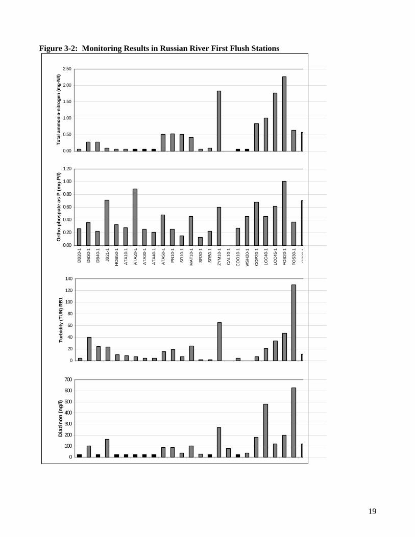
3.2 Major Findings 3.2.1 Data Limitations The quality of RRFF constituent measurements makes the Results good for practically any use, with exceptions; these exceptions are related to individual Result points and they are well-marked (flagged) in the Project File (see Section 4 and Appendix B for further information). Data interpretation, however, should be done with caution because of limited representativeness, both in time (we have only sampled a fraction of the entire storm event) and in space (we do not have comprehensive coverage of the watershed). Because we do not really know how well our samples represent RRFF, we can only use the data as a “spotlight” moving across the watershed and illuminating parts of it. However, the data we do have are reliable and the picture emerging from them is useful in targeting our next questions and generating valuable recommendations for future efforts. 3.2.2 Watershed-Scale Observations Figure 3-2 shows a set of four bar-graphs, each showing concentrations of one parameter as a function of Sample ID. Note that the naming convention used to generate Sample ID includes the Station ID and a serial number, and the results shown in these graph represent only the first Sample collected at

18

each Station, not all three. By placing the graphs one under the other in a way that they share the same Sample IDs, we can view the relationship between the different parameters as well. Figure 3-2 shows a high variability in concentrations at different watershed locations at the same time. It also indicates that areas with high concentrations of one constituent (parameter) are not necessarily a major source of other constituents (e.g., a “hot spot” for nutrients was not necessarily high in diazinon, high PO4 was not necessarily associated with high ammonia).

19

Figure 3-2: Monitoring Results in Russian River First Flush Stations

0.00

0.50

1.00

1.50

2.00

2.50

1 2 3 4 5 6 7 8 9 10 11 12 13 14 15 16 17 18 19 20 21 22 23 24 2

Tota

l am

mon

ia-n

itrog

en (m

g-N

/l)

0.00

0.20

0.40

0.60

0.80

1.00

1.20

DB2

0-1

DB3

0-1

DB4

0-1

JB21

-1

HO

B50-

1

ATA1

0-1

ATA2

0-1

ATA3

0-1

ATA4

0-1

ATA5

0-1

PN10

-1

SR10

-1

MAT

10-1

SR30

-1

SR50

-1

ZYM

10-1

CAL

10-1

CO

O10

-1

WSH

20-1

CO

P20-

1

LCC

40-1

LCC

45-1

FOS2

0-1

FOS3

0-1

GB2

01

Ort

ho-p

hosp

ate

as P

(mg-

P/l)

0

20

40

60

80

100

120

140

1 2 3 4 5 6 7 8 9 10 11 12 13 14 15 16 17 18 19 20 21 22 23 24 2

Turb

idity

(TU

N) R

B1

0

100

200

300

400

500

600

700

Dia

zino

n (n

g/l)

20

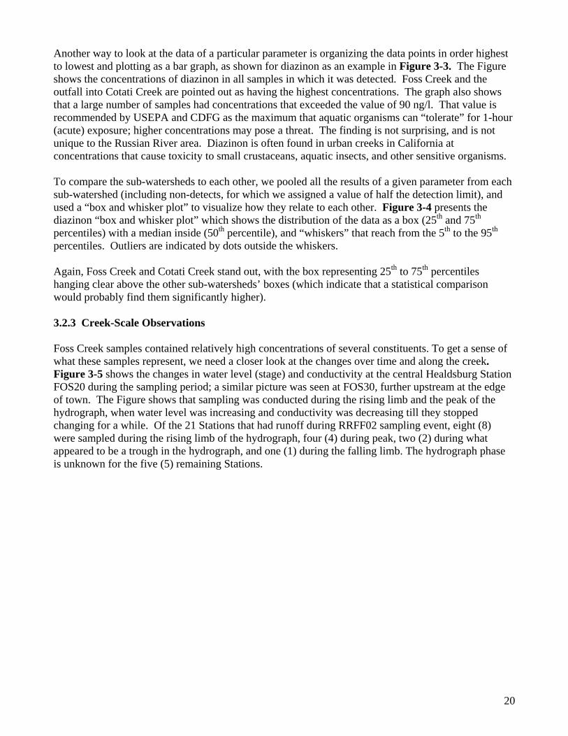
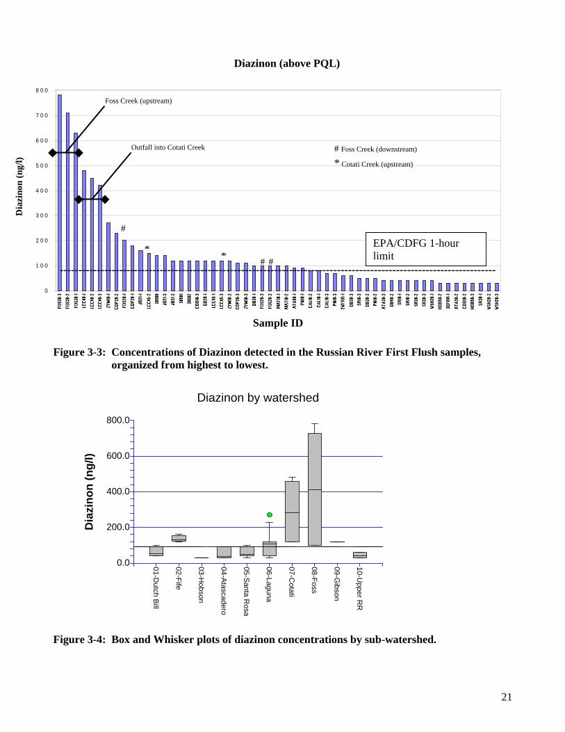
Another way to look at the data of a particular parameter is organizing the data points in order highest to lowest and plotting as a bar graph, as shown for diazinon as an example in Figure 3-3. The Figure shows the concentrations of diazinon in all samples in which it was detected. Foss Creek and the outfall into Cotati Creek are pointed out as having the highest concentrations. The graph also shows that a large number of samples had concentrations that exceeded the value of 90 ng/l. That value is recommended by USEPA and CDFG as the maximum that aquatic organisms can “tolerate” for 1-hour (acute) exposure; higher concentrations may pose a threat. The finding is not surprising, and is not unique to the Russian River area. Diazinon is often found in urban creeks in California at concentrations that cause toxicity to small crustaceans, aquatic insects, and other sensitive organisms. To compare the sub-watersheds to each other, we pooled all the results of a given parameter from each sub-watershed (including non-detects, for which we assigned a value of half the detection limit), and used a “box and whisker plot” to visualize how they relate to each other. Figure 3-4 presents the diazinon “box and whisker plot” which shows the distribution of the data as a box (25th and 75th percentiles) with a median inside (50th percentile), and “whiskers” that reach from the 5th to the 95th percentiles. Outliers are indicated by dots outside the whiskers. Again, Foss Creek and Cotati Creek stand out, with the box representing 25th to 75th percentiles hanging clear above the other sub-watersheds’ boxes (which indicate that a statistical comparison would probably find them significantly higher). 3.2.3 Creek-Scale Observations Foss Creek samples contained relatively high concentrations of several constituents. To get a sense of what these samples represent, we need a closer look at the changes over time and along the creek. Figure 3-5 shows the changes in water level (stage) and conductivity at the central Healdsburg Station FOS20 during the sampling period; a similar picture was seen at FOS30, further upstream at the edge of town. The Figure shows that sampling was conducted during the rising limb and the peak of the hydrograph, when water level was increasing and conductivity was decreasing till they stopped changing for a while. Of the 21 Stations that had runoff during RRFF02 sampling event, eight (8) were sampled during the rising limb of the hydrograph, four (4) during peak, two (2) during what appeared to be a trough in the hydrograph, and one (1) during the falling limb. The hydrograph phase is unknown for the five (5) remaining Stations.

21

Figure 3-3: Concentrations of Diazinon detected in the Russian River First Flush samples,

organized from highest to lowest.

Figure 3-4: Box and Whisker plots of diazinon concentrations by sub-watershed.

0.0

200.0

400.0

600.0

800.001-D

utch Bill

02-Fife

03-Hobson

04-Atascadero

05-Santa Rosa

06-Laguna

07-Cotati

08-Foss

09-Gibson

10-Upper R

R

Diazinon by watershed

Dia

zino

n (n

g/l)

D i a z i n o n - A b o v e P Q L

0

1 0 0

2 0 0

3 0 0

4 0 0

5 0 0

6 0 0

7 0 0

8 0 0

S a m p le ID

Dia

zino

n - p

pb

Foss Creek (upstream)

Outfall into Cotati Creek

* *

* Cotati Creek (upstream)

#

# #

# Foss Creek (downstream)

Dia

zino

n (n

g/l)

Diazinon (above PQL)

Sample ID

----------------------------------------------------------------------------------------------------------------------

EPA/CDFG 1-hour limit

22

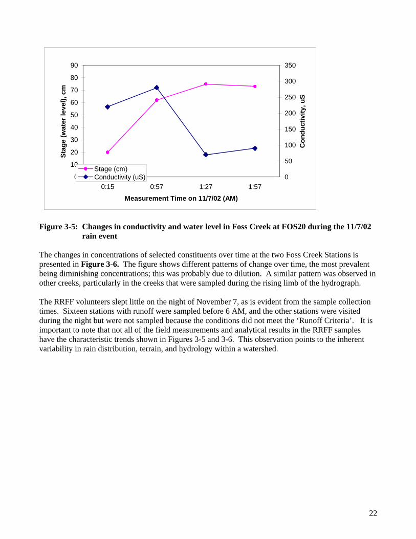
Figure 3-5: Changes in conductivity and water level in Foss Creek at FOS20 during the 11/7/02

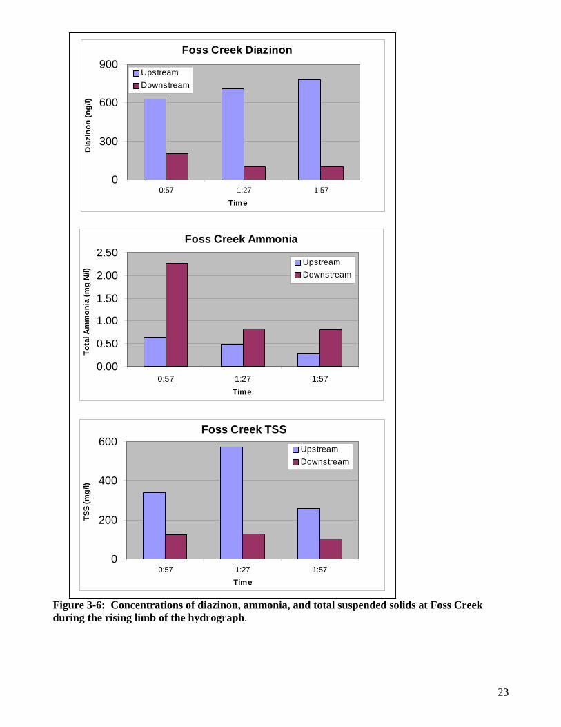
rain event The changes in concentrations of selected constituents over time at the two Foss Creek Stations is presented in Figure 3-6. The figure shows different patterns of change over time, the most prevalent being diminishing concentrations; this was probably due to dilution. A similar pattern was observed in other creeks, particularly in the creeks that were sampled during the rising limb of the hydrograph. The RRFF volunteers slept little on the night of November 7, as is evident from the sample collection times. Sixteen stations with runoff were sampled before 6 AM, and the other stations were visited during the night but were not sampled because the conditions did not meet the ‘Runoff Criteria’. It is important to note that not all of the field measurements and analytical results in the RRFF samples have the characteristic trends shown in Figures 3-5 and 3-6. This observation points to the inherent variability in rain distribution, terrain, and hydrology within a watershed.

0

10

20

30

40

50

60

70

80

90

0:15 0:57 1:27 1:57

Measurement Time on 11/7/02 (AM)

Stag

e (w

ater

leve

l), c

m

0

50

100

150

200

250

300

350

Con

duct

ivity

, uS

Stage (cm)Conductivity (uS)

23

Figure 3-6: Concentrations of diazinon, ammonia, and total suspended solids at Foss Creek during the rising limb of the hydrograph.

Foss Creek Diazinon

0

300

600

900

0:57 1:27 1:57Time

Dia

zino

n (n

g/l)

UpstreamDownstream

Foss Creek Ammonia

0.00

0.50

1.00

1.50

2.00

2.50

0:57 1:27 1:57Time

Tota

l Am

mon

ia (m

g N

/l)

UpstreamDownstream

Foss Creek TSS

0

200

400

600

0:57 1:27 1:57Time

TSS

(mg/

l)

UpstreamDownstream

24

4.0 Data Quality Overview There are many attributes of data quality, and each of them means something different about the data. It helps to break these attributes into major groups, dealing with different aspects separately. The following sections provides a discussion of RRFF data quality as related to the following:

1. Quality of the measurement (e.g., accuracy); 2. Sample integrity; 3. Fidelity of information transfer and data entry; 4. Reliability and validity; 5. Representativeness; and 6. Usability.

4.1 Measurement Quality RRFF data are reported with the range of error associated with each Result, so that any data user can ‘factor in’ the uncertainty when they use the data for decision-making. We communicate the error by providing measures of accuracy and precision, which describe how far we may have been from the ‘absolute true value’ (that’s accuracy) and how far our results are from each other when we repeat our measurements (precision). Measures of accuracy and precision are often lumped together to generate a cumulative range of error. The sensitivity of our methods also matters, so we have to specify the detection limit (the lowest value we can report with confidence that it is actually a positive result) and the resolution (the smallest increment that our method or instrument can discern). The instruments or kits we use to make the measurements will determine the ‘attainable’ quality, but in reality a lot depends on the skills and actions of the operators. For example, the resolution of our ammonia and phosphate kits was greatly improved when we used the kit’s reagents with an array of samples and a calibration curve, and read the absorbance in a spectrophotometer. The detection limits of these analyses were also improved (i.e., lowered), by using thick test tubes which provided for a longer light path within the spectrophotometer and enabled detection of significant signals at lower color intensity. Field and lab operators were given guidance and tools to Control, Check, Record, and Report (CCRR) the quality of their measurements and analyses. Essentially, ‘Control’ is about things we can do to improve accuracy and precision (resolution, detection limit, and range are usually a ‘given’ for a given instrument but there are ways to improve them as well, see above). ‘Check’ is for things we cannot control but need to know. ‘Record’ is about the language we use to express our findings and about entering these findings into the ‘placeholders’ on our forms or spreadsheet. ‘Report’ is about the way we calculate the measures of accuracy and precision so they can be shared with others. Note that each type of instrument or kit requires its unique CCRR actions (that cannot be generalized for all measurement devices), the step-by-step instructions for these actions were provided in the instrument-specific standard operating procedures (SOP). Detailed information regarding measurement quality by parameter or group of parameters, in the field and in the lab, is provided in Appendix B of this report and in the in the RRFF Project File (see Section 2.7 above). In a nutshell, measurement quality is partially known for selected field measurements (e.g., conductivity and pH) for which we have documentation, and is in the range of 10 to 20% error. Laboratory analyses were fully documented; the error around ammonia, ortho-phosphate, and TSS Results was 10% or less, while turbidity and diazinon data were associated with 10-20% error and nitrate bacterial counts were associated with up to 50% error (which is excellent for E. coli and total coliform data).

25

The sensitivity (resolution and detection limit) of RRFF data was within the measurement quality objectives set for each parameter and method, and was adequate for the purpose of monitoring (Appendix B). 4.2 Sample Integrity Sample integrity is about lack of contamination and lack of deterioration. We assure lack of contamination through a number of control actions; we decontaminate sampling equipment and keep everything clean to avoid contamination of the probes used for field measurements, the sampling devices, the sample containers, the lab reagents, etc. We prevent sample deterioration by keeping the samples in coolers or in the refrigerator at all times and by analyzing within the specified ‘holding time’. RRFF sampling and analyses work included application of all these control measures. To check sample integrity we collect and analyze equipment blanks (sampling devices, containers, and sample filtration devices), and we measure temperatures when relinquished at EPA lab. These checks showed that RRFF sample results were not due to contamination. To avoid contamination of bacterial samples within the coolers we used blue ice, and consequently the samples sent to EPA lab arrived at 10 C. This temperature is slightly higher than recommended shipping temperature, but the excursion from recommended temperature was very short (less than 2 hours) and probably did not compromise sample integrity. 4.3 Fidelity of information transfer and data entry Data ‘fidelity’ means correct transfer of information from observer to ‘scribe’ and correct recording during field work, as well as data copying and data entry into electronic formats later in the process. The fidelity of information transfer in the field has not been assessed; however it is not so relevant to the laboratory results generated with the samples. As for data entry, most field data was entered by citizen volunteers directly into the Project File and the review by the Scientific coordinator showed that it was entered with >99% fidelity. Raw data from RB1 in-house lab analysis was entered by citizen volunteers and RB1 Lab liaison into special worksheets, with >95% fidelity. 4.4 Reliability and Validity The credibility and validity of monitoring data go hand-in-hand in the way they are assessed, and they both require complete documentation of the measurements (instruments, QAQC, etc.), the station location, the sampling design, and other bits of essential information. Reliability implies honest reporting by field operators and a high probability that the reported value indeed falls within the range of error specified for it. Validity means the test, assay, or analysis used to collect the data was valid and that the target data quality objectives have been achieved. Note that knowledge about the quality of the measurement itself (see below) is essential for labeling a dataset ‘reliable and valid’. RRFF Results are associated with a high level of documentation, with very few ‘holes’ in the matrix of supporting information. Measurement quality is known for most of the data points. All the data have been reviewed, and each Result is presented to the users with qualifying information on the level of documentation, the extent of measurement error, and the data validation outcome. 4.5 Representativeness As mentioned above, RRFF data have limited representativeness, both in time (we have only sampled a fraction of the entire storm event) and in space (we do not have comprehensive coverage of the watershed). However, having datasets with three consecutive samples provides information about

26

what each sample represents within the sampling period. Likewise, having several stations along one waterway increases our understanding of what each Station represents within that creek. The principles used in planning for three consecutive samples and multiple creek locations can and should be utilized in designing future studies and ‘zooming in’ on particular segments of the Russian river Watershed. 4.6 Usability Most of the Results collected by RRFF teams are usable in the sense that they can answer some very relevant questions. They are comparable to other data sets in terms of sampling design and data quality, they are scientifically defensible, and they are reported and documented in formats that can be easily read, understood, and shared. For the regulators, these data – although they should not be used for litigation - provide information that will help prioritize future investigation. Local agencies in charge of pollution prevention can benefit from the knowledge when they allocate resources to management measures. The watershed groups can use the data to educate neighbors, students, and the community at large. Last but not least, information gleaned from the results can and should be used to design the next studies done in the watershed. 5.0 Summary and recommendations First Flush storm runoff samples were collected by citizen volunteers in 21 Stations in urban drainages within the Russian River watershed on 11/7/02. Five additional stations, representing base flows (non-runoff), were sampled as well. Sampling efforts yielded 80 samples which were analyzed for a number of constituents, including bacteria, nutrients, suspended solids, and the insecticide diazinon. The quality of RRFF constituent measurements makes the Results good for practically any use, with exceptions that are well-marked (flagged). RRFF data are of limited representativeness, both in time (only a fraction of the entire storm event was sampled) and in space (coverage of the watershed was not comprehensive). Therefore, data interpretation should be done with caution. Three urban drainages stood out as laced with potentially problematic concentrations of some stormwater constituents. The situation in other locations was not as severe, although several additional inputs of stormwater constituents have been identified. Phosphate and Nitrate were detected in the majority of samples tested; however their sources may be natural (these nutrients often run off pristine landscapes during the first runoff event after a long dry season). Suspended solids concentrations and bacterial counts were within the range normally encountered in urban runoff, and the presence of diazinon and ammonia pollution (i.e., at concentrations thought to pose a risk to aquatic life) is also familiar. The dataset provides an initial ‘big picture’ that can help develop some perspective on the occurrences of the major constituents. Information gleaned from this characterization effort can help citizens, local agencies, and regulators prioritize future management options. RRFF efforts brought together many professionals, and a network of technically-savvy folks has formed. It is recommended to maintain this network within the RRFF contact list and apply it to future monitoring efforts in the watershed.

27

Citizens participating in RRFF have learned that many monitoring activities are actually ‘doable’, they now feel empowered to proceed with monitoring in their localities with help from the local technical network folks. Observations and conclusions gleaned from the data can focus future efforts around a given area and to design additional studies tailored to answer specific questions. These additional studies can be performed by citizens. Examples: fine mapping of sub-basins; relationship between what was found in a creek during RRFF and what flows or stands in that creek during dry weather; what practices characterize that specific drainage; are there BMPs that work well; etc. It is highly recommended to consider the lessons learned when planning future efforts. For example, Study Design could benefit from a set of Stations focused around a small section of the watershed, and from a temporal sampling schedule that spans the entire hydrograph. Repetition of First Flush monitoring in subsequent years will help create a more robust body of information, even if conducted only in the urban sectors of the Russian River watershed. The citizens of the Russian River Watershed have expressed their wish to capture the first flush again in the fall of 2003. Interested parties are encouraged to contact the volunteer coordinator (see Appendix table A-2). 6.0 Glossary Accuracy: How close is our measurement to the real truth: the extent of agreement between an

observed value (measurement result) and the accepted, or true, value of the parameter being measured.

Accuracy Check: Comparison of the reading, or output, of a measurement device with a value believed

the ‘true’ value. The ‘true’ value may be represented by known natural conditions (e.g., freezing point) or by an established Standard. An ‘Accuracy Check’ is different from a Calibration, since it is only a comparison and does not result in an adjustment (calibration) of an instrument or procedure.

Blank (Sample): A sample that contains pure water and is analyzed concomitantly with a set of

environmental samples. Blanks usually include field blanks and trip blanks to assure that there was not contamination during sampling and shipping, as well as laboratory method blanks and reagent blanks, tested within the analytical procedures

Blue Ice (vs wet ice): A pre-frozen device used to chill objects (e.g., full sample containers), inside an

insulated chest, without melting. Calibration: The action of adjusting the readings of an instrument to have them match a ‘true’ value as

represented by known natural conditions (e.g., freezing point) or by a Standard Solution (e.g., Standard pH buffer).

Data Quality Objectives (DQOs): Statements about the level of uncertainty in data that a decision-

maker is willing to accept to support a particular decision. DQOs include measurement quality objectives (precision, accuracy, detection limit, and resolution) as well as measures of completeness, representativeness, and comparability.

28

Data Validation: The process to assure data meets requirements and quality objectives and that the test or analysis used to generate the data was valid.

Data Users: The group(s) that will be applying the monitoring results for decision making or other

purpose. Data users can include the monitors themselves as well as government agencies, schools, universities, businesses, watershed organizations, and community groups.

Database: A computerized system for managing, storing, and retrieving data. Diazinon: A wide-range insecticide used for control of pests in yards and gardens. Diazinon is highly

toxic to many species of crustaceans and aquatic insect larvae. Dissolved Oxygen (DO): Oxygen dissolved in water and available for living organisms to use for

respiration, usually expressed in milligrams per liter or percent of saturation. Duplicate Samples: two samples taken at the same time from the same site (but into separate

containers) that are carried through all assessment and analytical procedures in an identical manner. Duplicate samples are given separate (and unique) Sample IDs. Results of duplicate samples are used to evaluate the Reproducibility of the measurements.

Field Operator: The Project person who conducts monitoring activities in the field, including

measurements, calibrations and/or accuracy checks, and sampling. Hydrograph: a plot showing the stage (water level) in a creek as a function of time. The ‘storm

Hydrograph’ shows one or more peaks. Instrument: a probe, electrode, reagent kit, indicator strip, or any other type of device used for field or

laboratory measurements. Parameter: A property or substance to be measured within a medium. Parameters include properties

such acidity (pH) or electrical conductivity, particulates such as suspended solids or bacteria, and analytes such as ammonia or heavy metals.

pH: Numerical measure of the hydrogen ion concentration used to indicate the alkalinity or acidity of a

substance. Measured on a scale of 1.0 (acidic) to 14.0 (basic); 7.0 is neutral Precision: A measure of how close repeated measurements are to each other. Project: A data collection effort, performed by one or more organizational entities, which is limited in

space and time. Project File: An Excel workbook with multiple spreadsheets that include all the results, result

descriptors, and supporting documentation relevant to one Project. Replicate Samples: two or more test tubes taken from the same sample container and analyzed in

parallel, or repeated titrations of the same fixed sample (i.e., measurements relating to a common Sample ID). ‘Split samples’ are replicates because they originate from a common container and represent the same ‘chunk’ of water. Results of replicate samples are used to evaluate the Repeatability of the measurements.

29

Result: The outcome of a measurement or an observation. Results can be expressed in numbers, words (‘verbal categories’), or ranges or numbers (‘numeric range categories’).

Resolution: The smallest increment that can be discerned on the scale of a measuring device, or the

capability of a method to discriminate between measurement responses. Significant digits - digits in a numerical Result that have a number that is meaningful. In most cases

three significant digits are fine, e.g., 10.4 mg/l DO (all three digits are significant) or 1560 uS (the first three are significant, the last one provides the order of magnitude but the difference between zero and, say, 2, is not significant).

Split Samples - Two or more Replicates that have originated from a common Sample container and

thus represent the same ‘chunk’ of water. Split Samples are often used to compare performance of different laboratories, in what is commonly termed ‘round robin tests’.

Standard Operating Procedure (SOP): A written document providing step-by step instructions for

performing a procedure (sampling, measurement, or other). Standard Solution: A solution containing a known concentration of a substance, prepared or purchased

for use in the analytical laboratory or in the field. It is used in calibrations and in quality control checks on procedures and instruments. This category includes ‘Calibrator Standards’ used for calibration of adjustable pH and conductivity meters (etc.), usually as the ‘Resident Standards’ that each monitoring entity uses, as well as SRMs and ‘External Standards’ such as those used in regional Intercalibration Exercises. Each bottle of these types of Standards has to have a unique ID.

Total Suspended Solids (TSS): The amount of all particulate matter suspended in the water, expressed

as dry weight per volume, e.g., mg/l. Turbidity: A property of the water, often due to tiny particles suspended in it, that causes absorbance

of light and loss of clarity. Water Quality Parameters: Any of the measurable properties, qualities or contents of water. Wet Ice: Unpacked blocks or chunks of ice that yield water when melted. When used in ice chests to

cool environmental samples, the containers have to be protected from intrusion of melt water.

30

APPENDIX A Russian River First Flush station and participant information

Table A-1. Russian River First Flush Station Information. # on

Map Station ID Waterbody Latitude * Longitude * Station Location

Dutch Bill Creek sub-watershed 1 DB20 Dutch Bill Creek 38.43566 -122.97342 Camp Meeker/ Alliance Redwoods 2 DB30 Outfall into Dutch Bill

Creek 38.41070 -122.94939 Graton Rd @ Bohemian Hwy

3 DB40 Dutch Bill Creek 38.41072 -122.94876 Dutch Bill Hdwaters@ Graton Rd Fife Creek sub-watershed 4 JB21 Oufall into Fife Creek 38.50210 -123.00190 Fife Creek @ Highway 116

Hobson Creek sub-watershed 5 HOB50 Hobson Creek 38.51344 -122.93307 McPeak & Skyline Green Valley / Atascadero Creek sub-watershed 6 ATA10 Green Valley Creek 38.48332 -122.91551 Martinelli Rd 7 ATA20 Atascadero Creek 38.44431 -122.87700 Grren Valley Rd Bridge 8 ATA30 Graton Critch 38.43526 -122.87122 Graton Critch @ Railroad Ave 9 ATA40 Atascadero Creek 38.41091 -122.86178 Mill Station @ Atascadero 10 ATA50 Atascadero Creek 38.39747 -122.84820 Bodega Highway Mark West Springs sub-watershed 11 LTH Mark West Springs 38.49420 -122.85307 Laguna @ Trenton/Healdsburg Rd 12 PN10 Piner Creek 38.44853 -122.76941 Piner Crk @ Fulton Rd 13 SR10 Santa Rosa Creek 38.44172 -122.76948 Santa Rosa Crk @ Fulton Rd 14 MAT10 Matanzas Creek 38.43890 -122.69980 Doyle Park 15 SR30 Santa Rosa Creek 38.45120 -122.67978 Santa Rosa Crk @ Yulupa Ave 16 SR50 Santa Rosa Creek 38.45615 -122.63746 Santa Rosa Crk @ Melita Rd Laguna de Santa Rosa sub-watershed 17 LOR Laguna de Santa Rosa 38.42567 -122.82871 Laguna @ Occidental Rd

18 Zym10 Zymfin Creek 38.40668 -122.81990 Zymfin Creek @ Morris St 19 CAL10 Calder Creek 38.40391 -122.81021 Radota Trail Sebastopol 20 COO10 Cooper Creek 38.38814 -122.80311 Cooper Creek @ Cooper Road 21 LSP Laguna de Santa Rosa 38.35227 -122.74145 Laguna @ Sebatopol Rd 22 WSH20 Outfall into Washoe

Creek 38.32483 -122.73412 Vineyard Ditch @ Washoe Crk

23 COP20 Copeland Creek 38.34312 -122.71196 Copeland Creek @ Commerce Blvd 24 LCC40 Outfall into Cotati

Creek 38.32793 -122.70365 Cotati Creek north of E Cotati Ave

25 LCC45 Cotati Creek 38.32715 -122.70306 Cotati Creek @ E Cotati Ave Foss Creek sub-watershed 26 FOS20 Foss Creek 38.61111 -122.87188 Foss Creek Downtown 27 FOS30 Foss Creek 38.64313 -122.87190 Upper Foss Creek Gibson Creek sub-watershed 28 GB20 Gibson Creek 39.14539 -123.19202 Gibson Crk @ Gobbi St West Fork Russian River 29 2WFRR Russian River 39.23120 -123.20135 West Fork Russian River East Fork Russian River 30 3EFRR Russian River 39.24805 -123.12242 East Fork Russian River * Datum NAD83 / WGS84

31

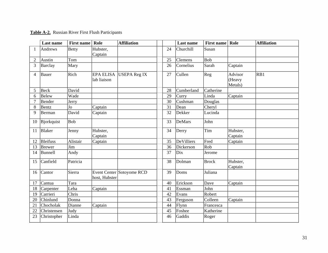
Table A-2. Russian River First Flush Participants

Last name First name Role Affiliation Last name First name Role Affiliation 1 Andrews Betty Hubster,

Captain 24 Churchill Susan

2 Austin Tom 25 Clemens Bob 3 Barclay Mary 26 Cornelius Sarah Captain

4 Bauer Rich EPA ELISA lab liaison

USEPA Reg IX 27 Cullen Reg Advisor (Heavy Metals)

RB1

5 Beck David 28 Cumberland Catherine 6 Belew Wade 29 Curry Linda Captain 7 Bender Jerry 30 Cushman Douglas 8 Bentz Jo Captain 31 Dean Cheryl 9 Berman David Captain 32 Dekker Lucinda

10 Bjorkquist Bob 33 DeMars John

11 Blaker Jenny Hubster, Captain

34 Derry Tim Hubster, Captain

12 Bleifuss Alistair Captain 35 DeVilliers Fred Captain 13 Brewer Jim 36 Dickerson Rob 14 Bunnell Andy 37 Dix Jerome

15 Canfield Patricia 38 Dolman Brock Hubster, Captain

16 Cantor Sierra Event Center host, Hubster

Sotoyome RCD 39 Doms Juliana

17 Cantua Tara 40 Erickson Dave Captain 18 Carpenter Leha Captain 41 Essman John 19 Carrieri Chris 42 Evans Robert 20 Chinlund Donna 43 Ferguson Colleen Captain 21 Chocholak Dianne Captain 44 Flynn Francesca 22 Christensen Judy 45 Foshee Katherine 23 Christopher Linda 46 Gaddis Roger

32

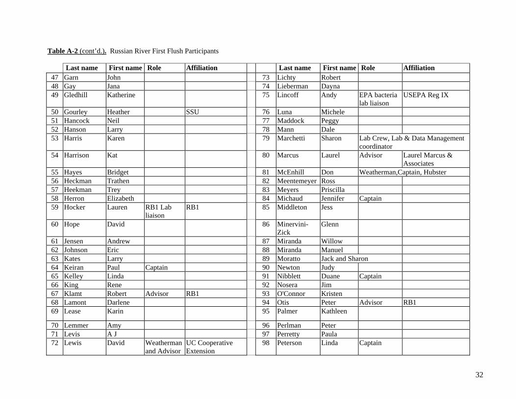
Table A-2 (cont’d.). Russian River First Flush Participants

Last name First name Role Affiliation Last name First name Role Affiliation 47 Garn John 73 Lichty Robert 48 Gay Jana 74 Lieberman Dayna 49 Gledhill Katherine 75 Lincoff Andy EPA bacteria

lab liaison USEPA Reg IX

50 Gourley Heather SSU 76 Luna Michele 51 Hancock Neil 77 Maddock Peggy 52 Hanson Larry 78 Mann Dale 53 Harris Karen 79 Marchetti Sharon Lab Crew, Lab & Data Management

coordinator 54 Harrison Kat 80 Marcus Laurel Advisor Laurel Marcus &

Associates 55 Hayes Bridget 81 McEnhill Don Weatherman,Captain, Hubster 56 Heckman Trathen 82 Meentemeyer Ross 57 Heekman Trey 83 Meyers Priscilla 58 Herron Elizabeth 84 Michaud Jennifer Captain 59 Hocker Lauren RB1 Lab

liaison RB1 85 Middleton Jess

60 Hope David 86 Minervini-Zick

Glenn

61 Jensen Andrew 87 Miranda Willow 62 Johnson Eric 88 Miranda Manuel 63 Kates Larry 89 Moratto Jack and Sharon 64 Keiran Paul Captain 90 Newton Judy 65 Kelley Linda 91 Nibblett Duane Captain 66 King Rene 92 Nosera Jim 67 Klamt Robert Advisor RB1 93 O'Connor Kristen 68 Lamont Darlene 94 Otis Peter Advisor RB1 69 Lease Karin 95 Palmer Kathleen

70 Lemmer Amy 96 Perlman Peter 71 Levis A J 97 Perretty Paula 72 Lewis David Weatherman

and Advisor UC Cooperative Extension

98 Peterson Linda Captain

33

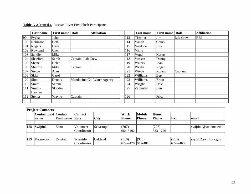
Table A-2 (cont’d.). Russian River First Flush Participants

Last name First name Role Affiliation Last name First name Role Affiliation 99 Pyeha John 113 Tischler Jim Lab Crew RB1 100 Robinson Beth 114 Vaugh Chuck 101 Rogers Dave 115 Verdone Lily 102 Rowland Cher 116 Visnu 103 Sandler Mike 117 Vogel Karen 104 Shaeffer Sarah Captain, Lab Crew 118 Vossen Denny 105 Shane Helen 119 Waters Joan 106 Sherron Mike Captain 120 Weeks Roger 107 Siegle Alan 121 Wiebe Roland Captain 108 Sklar Carol 122 Williams Bert 109 Slota Dennis Mendocino Co. Water Agency 123 Williams Brian 110 Smith Samuel 124 Wright Dale 111 Smith-

Heisters Skaidra 125 Zabinsky Ben

112 Stelter Wayne Captain 126 Fritz

Project Contacts Contact Last

name Contact First name

Contact Role

City

Work Phone

Mobile Phone

Home Phone

Fax

email

128 Swijtink Zeno Volunteer

Coordinator Sebastopol (707)

664-3192 (707)

823-1726 swijtink@sonoma.edu

129 Katznelson Revital Scientific

Coordinator Oakland (510)

622-2470(916) 947-4816

(510) 622-2460

rk@rb2.swrcb.ca.gov