Adversarial Generator-Encoder Networks

Dmitry Ulyanov 1 2 Andrea Vedaldi 3 Victor Lempitsky 1

AbstractWe present a new autoencoder-type architecture,that is trainable in an unsupervised mode, sus-tains both generation and inference, and has thequality of conditional and unconditional samplesboosted by adversarial learning. Unlike previ-ous hybrids of autoencoders and adversarial net-works, the adversarial game in our approach isset up directly between the encoder and the gen-erator, and no external mappings are trained inthe process of learning. The game objective com-pares the divergences of each of the real andthe generated data distributions with the canon-ical distribution in the latent space. We showthat direct generator-vs-encoder game leads to atight coupling of the two components, resultingin samples and reconstructions of a comparablequality to some recently-proposed more complexarchitectures.

1. IntroductionDeep architectures such as autoencoders (Bengio, 2009)and their variational counterparts (VAE) (Rezende et al.,2014; Kingma & Welling, 2013) can learn in an unsuper-vised manner a bidirectional mapping between data charac-terised by a complex distribution, such as natural images,and a much simpler latent space. Sampling an image re-duces then to drawing a sample in the latent space, which iseasy, and then mapping the latter to a data sample by apply-ing the learned generator function to it. Unfortunately, theperceptual quality of the generated samples remains rela-tively low. This is usually not a limitation of the neural net-work per-se, but rather of the simplistic loss functions usedto train it. In particular, simple losses are unable to properlyaccount for reconstruction ambiguities and result in blurrysamples (regression to the mean). By contrast, GenerativeAdversarial Networks (GANs) (Goodfellow et al., 2014)can learn complex loss functions as a part of the learning

1Skolkovo Institute of Science and Technology, Russia2Yandex, Russia 3University of Oxford, UK. Correspondence to:Dmitry Ulyanov <dmitry.ulyanov.msu@gmail.com>.

Source code is available athttps://github.com/DmitryUlyanov/AGE

process, which allows them to generate better quality sam-ples.

A disadvantage of GANs compared to autoencoders is that,in their original form, they are unidirectional: a GAN canonly generate a data sample from a latent space sample,but it cannot reverse this mapping. By contrast, in autoen-coders this inference process is carried by the encoder func-tion, which is learned together with the generator functionas part of the model. Therefore, there has been some inter-est in developing architectures that support both samplingand inference like autoencoders, while producing samplesof quality comparable to GAN. For example, the adversar-ial autoencoders of (Makhzani et al., 2015) augment au-toencoders with adversarial discriminators encouraging thealignment of distributions in the latent space, but the qual-ity of the generated samples does not always match GANs.The approach (Larsen et al., 2015) adds instead an adver-sarial loss to the reconstruction loss of the variational au-toencoder, with a sensible improvement in the quality of thesamples. The method of (Zhu et al., 2016) starts by learn-ing the decoder function as in GAN, and then learns a cor-responding encoder post-hoc. The adversarially-learned in-ference (ALI) approach, simultaneously proposed by (Don-ahue et al., 2016; Dumoulin et al., 2016), consider parallellearning of encoders and generators, whereas the distribu-tion of their input-output pairs are matched by an externaldiscriminator.

All such approaches (Makhzani et al., 2015; Larsen et al.,2015; Donahue et al., 2016; Dumoulin et al., 2016) add tothe encoder (or inference network) and decoder (or gener-ator) modules a discriminator module, namely an externalclassifier whose goal is to align certain distributions in thelatent or data space, or both.

In this paper, we propose a new approach for trainingencoder-generator pairs that uses an adversarial game be-tween the encoder and the generator, without the needto add an external discriminator. Our architecture, calledAdversarial Generator-Encoder Network (AGE Network),thus consists of only two feed-forward mappings (the en-coder and the generator). At the same time, AGE uses ad-versarial training to optimize the quality of the generatedsamples by matching their higher-level statistics to those ofreal data samples. Crucially, we demonstrate that it is pos-sible to use the encoder itself to extract the required statis-

arX

iv:s

ubm

it/18

5711

4 [

cs.C

V]

7 A

pr 2

017

Adversarial Generator-Encoder Networks

tics.

Adversarial training in AGE works as follows. First, theencoder is used to map both real and generated data sam-ples to the latent space, inducing in this space two empiri-cal data distributions. Since the aim of learning is to makegenerated and real data statistically indistinguishable, thethe generator is required to make these two latent distribu-tions identical. At the same time, the (adversarial) goal ofthe encoder is to construct a latent space where any statis-tical difference that can be discovered between the real andgenerated data is emphasized.

Importantly, AGE compares the latent distributions indi-rectly, by measuring their divergence to a reference canon-ical distribution (e.g. an i.i.d. uniform or normal vector).The evaluation of the game objective thus requires esti-mation of a divergence between distributions representedby sets of samples and an “easy” tractable distribution, forwhich we use a simple parametric or non-parametric esti-mator. The encoder is required to push the divergence ofthe real data down, a goal shared with VAE which makesthe distribution of real data in latent space a simple one.The generator is also required to push down the divergenceof the latent distribution corresponding to the generateddata; in this manner, the latent statistics of real and gener-ated data is encouraged to match. However, adversarially,the encoder is also encouraged to maximise the divergenceof the generated data.

The AGE adversarial game has a learning objective thatis quite different from the objectives used by existing ad-versarial training approaches. Since our goal is to avoidintroducing a discriminator function, this is partly out ofnecessity, since neither generator nor encoder can be usedas binary classifiers. Furthermore, introducing a binaryclassifier that classifies individual samples as generated orreal has known pitfalls such as mode collapse (Goodfellow,2017); instead, the discriminator should look at the statis-tics of multiple samples (Salimans et al., 2016). Our ap-proach does so by means of a new multi-sample objectivefor adversarial training.

As we show in the experiments, adversarial training withthe new objective is able to learn generators that produceshigh-quality samples even without reconstruction losses.Our new game objective can thus be used for stand-aloneadversarial learning. Our approach is evaluated on a num-ber of standard datasets. We include comparisons with theadversarially-learned inference (ALI) system of (Dumoulinet al., 2016) as well as the base generative adversarial ar-chitecture (Radford et al., 2015). We show that, for manydifferent datasets, AGE networks achieve comparable orbetter sampling and reconstruction quality than such alter-natives.

Generator g

Encoder e

Z

g(Z)

e(X)

e(g(Z))Latent space Data space

X

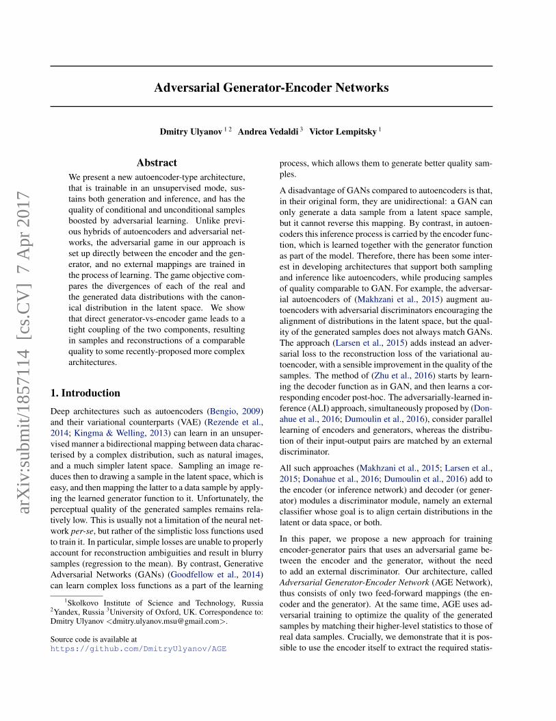
Figure 1. Our model (AGE network) has only two components:the generator g and the encoder e. The learning process adjuststheir parameters in order to align a simple distribution Z in thelatent space and the data distribution X . This is done by adver-sarial training, as updates for the generator aim to minimize thedivergence between e(g(Z)) and Z (aligning green with gray),while updates for the encoder aim to minimize the divergence be-tween e(X) (aligning blue with gray) and to maximize the diver-gence between e(g(Z)) and Z (shrink green “away” from gray).We demonstrate that such adversarial learning gives rise to high-quality generators that result in the close match between the realdistribution X and the generated distribution g(Z). Our learningcan also incorporate reconstruction losses to ensure that encoder-generator acts as autoencoder (section 2.2).

A note about notation: To ease the notation for a distribu-tion Y and a deterministic mapping f , we use the shorthandf(Y ) to denote the distribution associated with the randomvariable f(y), y ∼ Y .

2. Adversarial Generator-Encoder NetworksAdversarial Generator-Encoder (AGE) networks are com-posed of two parametric mappings that go in reverse direc-tions between the data space X and the latent space Z .The encoder eψ(x) with the learnable parameters ψ mapsdata space to latent space, while the generator gθ(z) withthe learnable parameters θ maps latent space to data space.

The goal of the training process for AGE is to align a realdata distributionX with a “fake” distribution gθ(Z) and es-tablish a reciprocal correspondence betweenX andZ at thesample level. The real data distributionX is represented bya sufficiently large number N of samples {x1,x2, ...xN}that follow this distribution; in the latent space, a simpledistribution Z is chosen, from which samples can be drawneasily. The training process corresponds to the tuning of theparameter sets ψ and θ. The process combines adversariallearning with the traditional minimization of reconstructionerrors in both spaces.

The simple form of the distribution Z allows uncondi-tional feed-forward sampling from the data distribution us-ing AGE networks by sampling z ∼ Z and computingx = gθ(z), exactly as it is done by sampling from a gen-erator in GANs. In our experiments, we pick the latentspace Z to be an M -dimensional sphere SM , and the la-tent distribution to be a uniform distribution on that sphere

Adversarial Generator-Encoder Networks

Z = Uniform(SM ). We have also conducted some experi-ments with the unit Gaussian distribution in the Euclideanspace and have obtained results comparable in quality.

In section 2.1 we introduce a game objective for which eachsaddle g delivers alignment g(Z) = X . We then augmentsit with additional terms that encourage the reciprocity of eand g in section 2.2. Section 2.3 describes the details of thelearning process for the introduced game.

2.1. Adversarial distribution alignment

The conventional approach to aligning two distributions isimplemented in existing GAN-based systems via an ad-versarial game based around ratio estimation (Goodfellowet al., 2014). The ratio estimation is performed by repeatedfitting of the binary classifier that distinguishes between thetwo distributions (corresponding to real and generated sam-ples). Here, we propose an alternative approach avoidingsome of the pitfalls of the conventional GANs such as modecollapse.

Our primary goal is to find generators that produce distri-butions in the data space g(Z) that are close to the truedata distribution X . However, direct matching of the dis-tributions in a high-dimensional data space can be verychallenging, thus we would like to limit ourself to com-paring only distributions defined in the latent space. In thefollowing derivations, we therefore introduce a divergencemeasure ∆(P‖Q) between distributions defined in the la-tent space Z . We only require this divergence to be non-negative and zero if and only if the distributions are iden-tical ∆(P‖Q) = 0 ⇐⇒ P = Q (triangle inequality andsymmetry property should not necessarily hold). An en-coder e maps distributions X and g(Z) in the latent spaceto the distributions e(X) and e(g(Z)) in the latent space.Below, we show how to design an adversarial game be-tween e and g that ensures the alignment of g(Z) = Xin the data space, while only evaluating divergences in thelatent space.

In the theoretical analysis below, we assume that consid-ered encoders and decoders span the class of all measur-able mappings between the corresponding spaces. Suchassumption (often referred to as non-parametric limit) isjustified by universality of neural networks (Hornik et al.,1989). We further make an assumption that there exists atleast one “perfect” generator that matches the data distribu-tion, i.e. ∃g0 : g0(Z) = X .

We start by considering a simple game with objective de-fined as:

maxe

mingV1(g, e) = ∆( e(g(Z))‖e(X) ) . (1)

As the following theorem shows, perfect generators formsaddle points (Nash equilibria) of the game (1) and all sad-

dle points of the game (1) are based on perfect generators.

Theorem 1. A pair (g∗, e∗) forms a saddle point of thegame (1) if and only if the generator g∗ matches the datadistribution, i.e. g∗(Z) = X .

The proof of the theorem is given in the appendix.

While the game (1) is sufficient for aligning distributionsin the data space, finding its saddle points is complicatedby the need to compare the two general-form distributionsgiven in the form of samples. This is aided by redesigningthe game as follows:

maxe

mingV2(g, e) = ∆(e(g(Z))‖Y )−∆(e(X)‖Y ). (2)

Here Y is a fixed distribution in the latent space. Im-portantly, as the following theorem demonstrates, the newgame still retains the connection between generators thatalign fake and real distributions and saddle points.

Theorem 2. If a pair (g∗, e∗) is a saddle point of game(2) then the generator g∗ matches the data distribution, i.e.g∗(Z) = X . Conversely, if the generator g∗ matches thedata distribution, then for some e∗ the pair (g∗, e∗) is asaddle point of (2).

The proof is given in the appendix.

The important benefit of the new game formulation (2) isthat the model distributions e(g(Z)) and e(X) are nowcompared with a fixed Y . By picking Y suitably, we canensure that the new divergence evaluations are more stablethan a direct comparison ∆( e(g(Z))‖e(X) ), as distribu-tions e(g(Z)) and e(X) are defined implicitly (we do nothave access to the distributions directly, but can only sam-ple from them).

Conveniently, one can pick the target distribution Y to co-incide with the “canonical”(source) distribution Z, and wedo so in all our experiments and further derivations. WithY = Z the game objective (2) can be upgraded with recon-struction losses and permits convenient stochastic approxi-mation as described in section 2.3.

One could also interpret the game (2) as the comparisonbetween the two distributions in the data space via compar-ison of certain statistics extracted by the encoders. Sim-ilarly to conventional GANs, these statistics are not fixedbut evolve in the process of the game. In our approach thestatistics have the form F (Q) = ∆(e(Q)‖Y ) for a givendistribution Q in the data space and a fixed distribution Yin the latent space. The statistics thus map a data spacedistribution into the latent space and then measure its di-vergence with the distribution Y .

We note that even away from the saddle point, the mini-mization ming V2(g, e) for some fixed e does not have a

Adversarial Generator-Encoder Networks

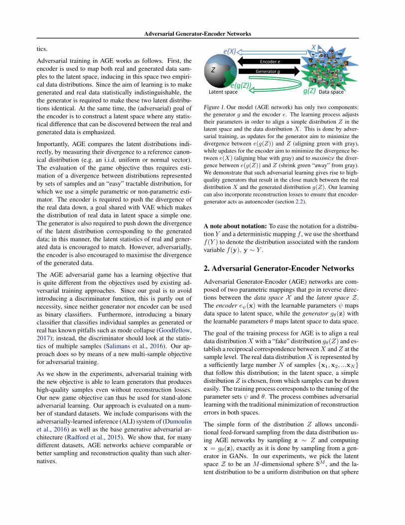
(a) Real (b) DCGAN (c) Ours (game 2) (d) Ours (full)

Figure 2. We compare CIFAR10 samples from DCGAN (Radford et al., 2015) (b) to the samples generated using our ablated modeltrained without reconstruction terms in (). The model, trained with the reconstruction terms is still able to produce diverse samples (d),but also allows inference (Figure 3).

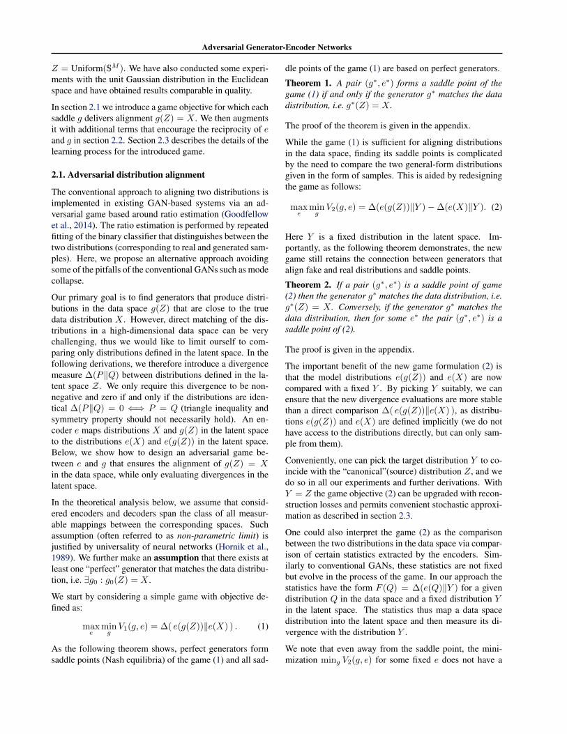
(a) Ours. (b) ALI (Dumoulin et al., 2016).

Figure 3. Comparison in reconstruction quality to ALI (Dumoulinet al., 2016) for the CIFAR10 dataset. For both figures real ex-amples are shown in odd columns and their reconstructions areshown in the even columns. The real examples come from test setand were never observed by the model during training.

collapsing tendency for many reasonable divergences (e.g.KL-divergence). Indeed, any collapsed distribution wouldinevitably lead to a very high value of the first term in (2).Thus, unlike GANs, our approach can optimize the gener-ator for a fixed adversary till convergence and obtain non-degenerate solution. On the other hand, the maximizationmaxe V2(g, e) for some fixed g can lead to +∞ score forsome divergences.

2.2. Reconstruction losses

While the previous derivation demonstrates that X andg(Z) can get aligned by adversarial learning, such align-ment does not necessarily entails reciprocity of the e and gmappings at the level of individual samples. Such sample-level reciprocity is not needed if we only need highly-realistic samples from the generator, however it is desirableif good reconstructions from the composition of encoderand generator are sought.

The sample-level reciprocity can be measured either in thelatent space or in the data space. This gives rise to the twoloss functions:

LX (gθ, eψ) = Ex∼X‖x− gθ(eψ(x)

)‖2 , (3)

LZ(gθ, eψ) = Ez∼Z‖z− eψ(gθ(z)

)‖2 . (4)

Both losses (3) and (4) thus measure the reconstruction er-ror and their minimization ensures the reciprocity of thetwo mappings. The loss (3) is the traditional loss usedwithin autoencoders.

As we aim to improve game (2), we may want to under-stand if both losses (3) and (4) should be used or one ofthem would be sufficient in theory. The answer is given bythe following statement:

Theorem 3. Let the two distributions W and Q bealigned by the mapping f (i.e. f(W ) = Q) and letEw∼W ‖w − h

(f(w)

)‖2 = 0. Then, for w ∼ W and

q ∼ Q, we have w = h(f(w)) and q = f(h(q)) almostcertainly, i.e. the mappings f and h invert each other al-most everywhere on the supports of W and Q. More, Q isaligned with W by h: h(Q) = W .

The proof is given in the appendix.

Recall that theorem 2 establishes that the solution (saddlepoint) of game (2) aligns distributions in the data space.Then, following theorem 3, adding the latent space loss (4)to the objective (2) is sufficient to ensure reciprocity.

2.3. Training AGE networks

Based on the theoretical analysis derived in the previoussubsections, we now suggest the approach to the joint train-ing of the generator in the encoder within the AGE net-works. As in the case of GAN training, we set up the learn-ing process for an AGE network as a game with the iterativeupdates over the parameters θ and ψ that are driven by the

Adversarial Generator-Encoder Networks

optimization of different objectives. In general, the opti-mization process combines the maximin game for the func-tional (2) with the optimization of the reciprocity losses (3)and (4).

In particular, we use the following game objectives for thegenerator and the encoder:

θ = arg minθ

(V2(gθ, eψ) + λLZ(gθ, eψ))

), (5)

ψ = arg maxψ

(V2(gθ, eψ)− µLX (gθ, eψ))) , (6)

where ψ and θ denote the value of the encoder and genera-tor parameters at the moment of the optimization and λ, µis a user-defined parameter. Note that both objectives (5),(6) include only one of the reconstruction losses. Specifi-cally the generator objective includes only the latent spacereconstruction loss. In the experiments, we found that theomission of the other reconstruction loss (in the data space)is important to avoid possible blurring of the generator out-puts that is characteristic to autoencoders. Similarly toGANs in (5), (6) we perform only several steps toward op-timum at each iteration, thus alternating between generatorand encoder updates.

By maximizing the difference between ∆(eψ(gθ(Z))‖Z)and ∆(eψ(X)‖Z), the optimization process (6) focuses onthe maximization of the mismatch between the real datadistribution X and the distribution of the samples from thegenerator gθ(Z). Informally speaking, the optimization (6)forces the encoder to find the mapping that aligns real datadistribution X with the target distribution Z, while map-ping non-real (synthesized data) g(Z) away from Z. WhenZ is a uniform distribution on a sphere, the goal of the en-coder would be to uniformly spread the real data over thesphere, while cramping as much of synthesized data as pos-sible together assuring non-uniformity of the distributioneψ(gθ(Z)

).

Any differences (misalignment) between the two distribu-tions are thus amplified by the optimization process (6) andforces the optimization process (5) to focus specifically onremoving these differences. Since the misalignment be-tween X and g(Z) is measured after projecting the twodistributions into the latent space, the maximization of thismisalignment makes the encoder to compute features thatdistinguish the two distributions.

3. Experiments3.1. Implementation details

Network architectures: In our experiments the generatorand the encoder networks have a similar structure to thegenerator and the discriminator in DCGAN (Radford et al.,2015). As our encoder should produce a vector instead ofa single number we modify the DCGAN’s discriminator

accordingly, expanding the last layer output to M dimen-sions. We also replace the sigmoid at the end with the nor-malization layer which projects the points onto the sphere.

Divergence measure: We use the following expression tomeasure the divergence between a distribution Q in the la-tent space and the distribution Z (which is the uniform dis-tribution on the M -dimensional sphere SM ):

∆(Q‖U(SM )) = KL(Q‖N (0, I))− C . (7)

Here,N (0, I) is the zero-mean unit-variance Gaussian dis-tribution in the embedding space RM , and the constant Cequals C = KL(U(SM )‖N (0, I)). Since the uniform dis-tribution on the sphere minimizes the KL-divergence withthe unit Gaussian out of all distributions on the sphere, theexpression (7) is valid (is non-negative, and equals zeroonly for Q = Z).

To measure the value KL(Q‖N (0, I)) for a mini-batchof examples, we used a parametric estimator, where aGaussian in the embedded space is fitted to the mini-batch and the KL-divergence between Gaussians is com-puted analytically. Having a set of M dimensionalsamples qi∼Q, i = 1, . . . , N with a component-wise mean m: mj = 1

N

∑Ni=1 qij and variance s:

sj = 1N

∑Ni=1(qij −mj)

2, the KL-divergence is approxi-mated with:

KL(Y ‖N (0, I)) ≈ −M2

+

M∑j=1

s2j +m2

j

2− log(sj) . (8)

We tried both the parametric version from above and thenon-parametric version based on Kozachenko-Leonenkoestimator (Kozachenko & Leonenko, 1987). Both versionsworked equally well, and we used a simpler parametric es-timator in the presented experiments.

Controlling the training process: while training the mod-els we ensure that the generator’s latent distribution staysas close to uniform on the sphere as possible. It is easiestto examine component-wise mean and variance of e(g(Z))for that purpose, as the mean should stay close to zero whilevariance should be approximately 1/dim(Z).

Hyper-parameters: We use ADAM (Kingma & Ba, 2014)optimizer with the learning rate of 0.0002. We perform twogenerator updates per one encoder update for all datasets.For each dataset we tried λ ∈ {500, 1000, 2000} andpicked the best one. We ended up using µ = 10 for alldatasets. The dimensionality M of the latent space wasmanually set according to the complexity of the dataset.We thus used M = 10 for MNIST, M = 64 for CelebAand SVHN datasets, and M = 128 for the most complexdatasets of Tiny ImageNet and CIFAR.

Adversarial Generator-Encoder Networks

(a) Real images. (b) Ours (samples). (c) Ours reconstructions. (d) ALI reconstructions.

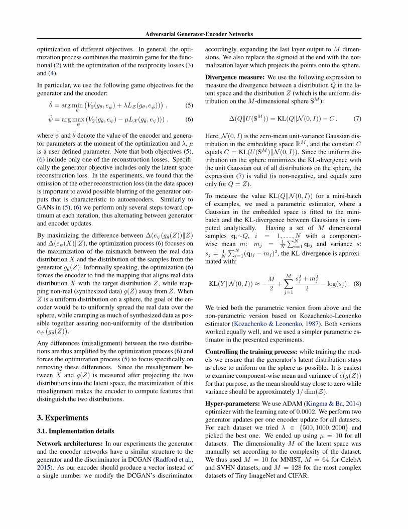
Figure 4. Samples (b) and reconstructions (c) for Tiny ImageNet dataset (top) and SVHN dataset (bottom). The results of ALI (Du-moulin et al., 2016) on the same datasets are shown in (d). In (c,d) odd columns show real examples and even columns show theirreconstructions. Qualitatively, our method seems to obtain more accurate reconstructions than ALI (Dumoulin et al., 2016), especiallyon the Tiny ImageNet dataset, while having samples of similar visual quality.

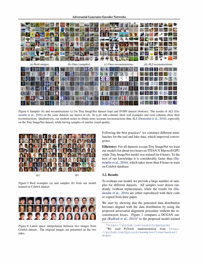
(a) (b)

Figure 5. Real examples (a) and samples (b) from our modeltrained on CelebA dataset.

Figure 6. Latent space interpolation between two images fromCelebA dataset. The original images are presented on the twosides.

Following the best practices1 we construct different mini-batches for the real and fake data, which improved conver-gence.

Efficiency: For all datasets except Tiny ImageNet we trainour models for about two hours on TITAN X Maxwell GPUwhile Tiny ImageNet model was trained for 6 hours. To thebest of our knowledge it is considerably faster than (Du-moulin et al., 2016), which takes more than 8 hours to trainon CelebA database.

3.2. Results

To evaluate our model, we provide a large number of sam-ples for different datasets. All samples were drawn ran-domly (without replacement), while the results for (Du-moulin et al., 2016) are either reproduced with their codeor copied from their paper.

We start by showing that the generated data distributionbecomes aligned with the data distribution by using theproposed adversarial alignment procedure without the re-construction losses. Figure 2 compares a DCGAN out-put (Radford et al., 2015)2 to the proposed model trained

1https://github.com/soumith/ganhacks2We used PyTorch implementation from https:

//github.com/pytorch/examples/tree/master/dcgan

Adversarial Generator-Encoder Networks

Orig. AGE ALI VAE Orig. AGE ALI VAE Orig. AGE ALI VAE Orig. AGE ALI VAE

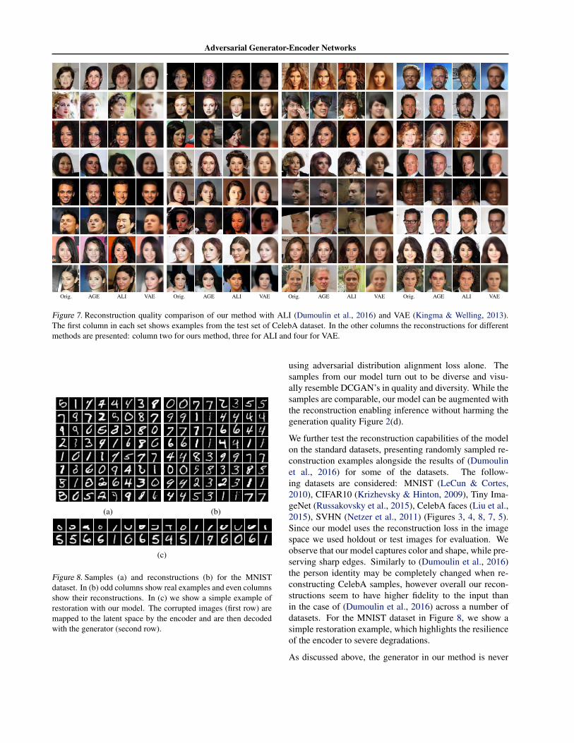
Figure 7. Reconstruction quality comparison of our method with ALI (Dumoulin et al., 2016) and VAE (Kingma & Welling, 2013).The first column in each set shows examples from the test set of CelebA dataset. In the other columns the reconstructions for differentmethods are presented: column two for ours method, three for ALI and four for VAE.

(a) (b)

(c)

Figure 8. Samples (a) and reconstructions (b) for the MNISTdataset. In (b) odd columns show real examples and even columnsshow their reconstructions. In (c) we show a simple example ofrestoration with our model. The corrupted images (first row) aremapped to the latent space by the encoder and are then decodedwith the generator (second row).

using adversarial distribution alignment loss alone. Thesamples from our model turn out to be diverse and visu-ally resemble DCGAN’s in quality and diversity. While thesamples are comparable, our model can be augmented withthe reconstruction enabling inference without harming thegeneration quality Figure 2(d).

We further test the reconstruction capabilities of the modelon the standard datasets, presenting randomly sampled re-construction examples alongside the results of (Dumoulinet al., 2016) for some of the datasets. The follow-ing datasets are considered: MNIST (LeCun & Cortes,2010), CIFAR10 (Krizhevsky & Hinton, 2009), Tiny Ima-geNet (Russakovsky et al., 2015), CelebA faces (Liu et al.,2015), SVHN (Netzer et al., 2011) (Figures 3, 4, 8, 7, 5).Since our model uses the reconstruction loss in the imagespace we used holdout or test images for evaluation. Weobserve that our model captures color and shape, while pre-serving sharp edges. Similarly to (Dumoulin et al., 2016)the person identity may be completely changed when re-constructing CelebA samples, however overall our recon-structions seem to have higher fidelity to the input thanin the case of (Dumoulin et al., 2016) across a number ofdatasets. For the MNIST dataset in Figure 8, we show asimple restoration example, which highlights the resilienceof the encoder to severe degradations.

As discussed above, the generator in our method is never

Adversarial Generator-Encoder Networks

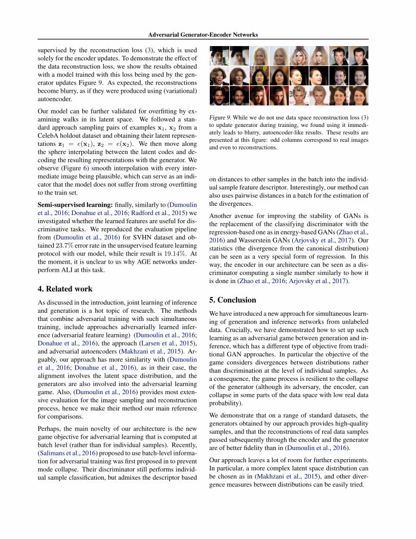
supervised by the reconstruction loss (3), which is usedsolely for the encoder updates. To demonstrate the effect ofthe data reconstruction loss, we show the results obtainedwith a model trained with this loss being used by the gen-erator updates Figure 9. As expected, the reconstructionsbecome blurry, as if they were produced using (variational)autoencoder.

Our model can be further validated for overfitting by ex-amining walks in its latent space. We followed a stan-dard approach sampling pairs of examples x1, x2 from aCelebA holdout dataset and obtaining their latent represen-tations z1 = e(x1), z2 = e(x2). We then move alongthe sphere interpolating between the latent codes and de-coding the resulting representations with the generator. Weobserve (Figure 6) smooth interpolation with every inter-mediate image being plausible, which can serve as an indi-cator that the model does not suffer from strong overfittingto the train set.

Semi-supervised learning: finally, similarly to (Dumoulinet al., 2016; Donahue et al., 2016; Radford et al., 2015) weinvestigated whether the learned features are useful for dis-criminative tasks. We reproduced the evaluation pipelinefrom (Dumoulin et al., 2016) for SVHN dataset and ob-tained 23.7% error rate in the unsupervised feature learningprotocol with our model, while their result is 19.14%. Atthe moment, it is unclear to us why AGE networks under-perform ALI at this task.

4. Related workAs discussed in the introduction, joint learning of inferenceand generation is a hot topic of research. The methodsthat combine adversarial training with such simultaneoustraining, include approaches adversarially learned infer-ence (adversarial feature learning) (Dumoulin et al., 2016;Donahue et al., 2016), the approach (Larsen et al., 2015),and adversarial autoencoders (Makhzani et al., 2015). Ar-guably, our approach has more similarity with (Dumoulinet al., 2016; Donahue et al., 2016), as in their case, thealignment involves the latent space distribution, and thegenerators are also involved into the adversarial learninggame. Also, (Dumoulin et al., 2016) provides most exten-sive evaluation for the image sampling and reconstructionprocess, hence we make their method our main referencefor comparisons.

Perhaps, the main novelty of our architecture is the newgame objective for adversarial learning that is computed atbatch level (rather than for individual samples). Recently,(Salimans et al., 2016) proposed to use batch-level informa-tion for adversarial training was first proposed in to preventmode collapse. Their discriminator still performs individ-ual sample classification, but admixes the descriptor based

Figure 9. While we do not use data space reconstruction loss (3)to update generator during training, we found using it immedi-ately leads to blurry, autoencoder-like results. These results arepresented at this figure: odd columns correspond to real imagesand even to reconstructions.

on distances to other samples in the batch into the individ-ual sample feature descriptor. Interestingly, our method canalso uses pairwise distances in a batch for the estimation ofthe divergences.

Another avenue for improving the stability of GANs isthe replacement of the classifying discriminator with theregression-based one as in energy-based GANs (Zhao et al.,2016) and Wasserstein GANs (Arjovsky et al., 2017). Ourstatistics (the divergence from the canonical distribution)can be seen as a very special form of regression. In thisway, the encoder in our architecture can be seen as a dis-criminator computing a single number similarly to how itis done in (Zhao et al., 2016; Arjovsky et al., 2017).

5. ConclusionWe have introduced a new approach for simultaneous learn-ing of generation and inference networks from unlabeleddata. Crucially, we have demonstrated how to set up suchlearning as an adversarial game between generation and in-ference, which has a different type of objective from tradi-tional GAN approaches. In particular the objective of thegame considers divergences between distributions ratherthan discrimination at the level of individual samples. Asa consequence, the game process is resilient to the collapseof the generator (although its adversary, the encoder, cancollapse in some parts of the data space with low real dataprobability).

We demonstrate that on a range of standard datasets, thegenerators obtained by our approach provides high-qualitysamples, and that the reconstrunctions of real data samplespassed subsequently through the encoder and the generatorare of better fidelity than in (Dumoulin et al., 2016).

Our approach leaves a lot of room for further experiments.In particular, a more complex latent space distribution canbe chosen as in (Makhzani et al., 2015), and other diver-gence measures between distributions can be easily tried.

Adversarial Generator-Encoder Networks

ReferencesArjovsky, Martın, Chintala, Soumith, and Bottou, Leon.

Wasserstein GAN. CoRR, abs/1701.07875, 2017.

Bengio, Yoshua. Learning deep architectures for AI. Foun-dations and Trends in Machine Learning, 2(1):1–127,2009.

Donahue, Jeff, Krahenbuhl, Philipp, and Darrell, Trevor.Adversarial feature learning. CoRR, abs/1605.09782,2016.

Dumoulin, Vincent, Belghazi, Ishmael, Poole, Ben, Lamb,Alex, Arjovsky, Martın, Mastropietro, Olivier, andCourville, Aaron C. Adversarially learned inference.CoRR, abs/1606.00704, 2016.

Goodfellow, Ian J. NIPS 2016 tutorial: Generative adver-sarial networks. CoRR, abs/1701.00160, 2017. URLhttp://arxiv.org/abs/1701.00160.

Goodfellow, Ian J., Pouget-Abadie, Jean, Mirza, Mehdi,Xu, Bing, Warde-Farley, David, Ozair, Sherjil,Courville, Aaron C., and Bengio, Yoshua. Generativeadversarial nets. In Proc. NIPS, pp. 2672–2680, 2014.

Hornik, Kurt, Stinchcombe, Maxwell, and White,Halbert. Multilayer feedforward networks areuniversal approximators. Neural Networks, 2(5):359 – 366, 1989. ISSN 0893-6080. doi:http://dx.doi.org/10.1016/0893-6080(89)90020-8. URLhttp://www.sciencedirect.com/science/article/pii/0893608089900208.

Kingma, Diederik P. and Ba, Jimmy. Adam: A method forstochastic optimization. CoRR, abs/1412.6980, 2014.

Kingma, Diederik P. and Welling, Max. Auto-encodingvariational bayes. CoRR, abs/1312.6114, 2013.

Kozachenko, L. F. and Leonenko, N. N. Sample estimateof the entropy of a random vector. Probl. Inf. Transm.,23(1-2):95–101, 1987.

Krizhevsky, Alex and Hinton, Geoffrey. Learning multiplelayers of features from tiny images. 2009.

Larsen, Anders Boesen Lindbo, Sønderby, Søren Kaae,and Winther, Ole. Autoencoding beyond pixels using alearned similarity metric. CoRR, abs/1512.09300, 2015.

LeCun, Yann and Cortes, Corinna. MNIST handwrittendigit database. 2010. URL http://yann.lecun.com/exdb/mnist/.

Liu, Ziwei, Luo, Ping, Wang, Xiaogang, and Tang, Xiaoou.Deep learning face attributes in the wild. In ICCV, pp.3730–3738. IEEE Computer Society, 2015.

Makhzani, Alireza, Shlens, Jonathon, Jaitly, Navdeep, andGoodfellow, Ian J. Adversarial autoencoders. CoRR,abs/1511.05644, 2015. URL http://arxiv.org/abs/1511.05644.

Marzouk, Youssef, Moselhy, Tarek, Parno, Matthew, andSpantini, Alessio. An introduction to sampling via mea-sure transport. arXiv preprint arXiv:1602.05023, 2016.

Netzer, Yuval, Wang, Tao, Coates, Adam, Bissacco,Alessandro, Wu, Bo, and Ng, Andrew Y. Reading digitsin natural images with unsupervised feature learning.In NIPS Workshop on Deep Learning and Unsuper-vised Feature Learning 2011, 2011. URL http://ufldl.stanford.edu/housenumbers/nips2011_housenumbers.pdf.

Owen, G. Game Theory. Academic Press, 1982. ISBN9780125311502. URL https://books.google.ru/books?id=pusfAQAAIAAJ.

Radford, Alec, Metz, Luke, and Chintala, Soumith. Unsu-pervised representation learning with deep convolutionalgenerative adversarial networks. CoRR, abs/1511.06434,2015.

Rezende, Danilo Jimenez, Mohamed, Shakir, and Wier-stra, Daan. Stochastic backpropagation and approxi-mate inference in deep generative models. arXiv preprintarXiv:1401.4082, 2014.

Russakovsky, Olga, Deng, Jia, Su, Hao, Krause, Jonathan,Satheesh, Sanjeev, Ma, Sean, Huang, Zhiheng, Karpa-thy, Andrej, Khosla, Aditya, Bernstein, Michael S.,Berg, Alexander C., and Li, Fei-Fei. Imagenet largescale visual recognition challenge. International Jour-nal of Computer Vision, 115(3):211–252, 2015.

Salimans, Tim, Goodfellow, Ian J., Zaremba, Wojciech,Cheung, Vicki, Radford, Alec, and Chen, Xi. Improvedtechniques for training gans. In Advances in Neural In-formation Processing Systems 29: Annual Conferenceon Neural Information Processing Systems 2016, De-cember 5-10, 2016, Barcelona, Spain, pp. 2226–2234,2016.

Villani, Cedric. Optimal transport: old and new, volume338. Springer Science & Business Media, 2008.

Zhao, Junbo Jake, Mathieu, Michael, and LeCun, Yann.Energy-based generative adversarial network. CoRR,abs/1609.03126, 2016. URL http://arxiv.org/abs/1609.03126.

Zhu, Jun-Yan, Krahenbuhl, Philipp, Shechtman, Eli, andEfros, Alexei A. Generative visual manipulation on thenatural image manifold. In Proceedings of EuropeanConference on Computer Vision (ECCV), 2016.

Adversarial Generator-Encoder Networks

A. AppendixLet X and Z be distributions defined in the data and thelatent spaces X , Z correspondingly. We assume X and Zare such, that there exists an invertible almost everywherefunction e which transforms the latent distribution into thedata one g(Z) = X . This assumption is weak, since forevery atomless (i.e. no single point carries a positive mass)distributionsX , Z such invertible function exists. For a de-tailed discussion on this topic please refer to (Villani, 2008;Marzouk et al., 2016). Since Z is up to our choice simplysetting it to Gaussian distribution (forZ = RM ) or uniformon sphere for (Z = SM ) is good enough.

Lemma A.1. Let X and Y to be two distributions definedin the same space. The distributions are equal X = Yif and only if e(X) = e(Y ) holds for for any measurablefunction e : X → Z .

Proof. It is obvious, that if X = Y then e(X) = e(Y ) forany measurable function e.

Now let e(X) = e(Y ) for any measurable e. To show thatX = Y we will assume converse: X 6= Y . Then thereexists a set B ∈ FX , such that 0 < PX(B) 6= PY (B)and a function e, such that corresponding set C = e(B)has B as its preimage B = e−1(C). Then we havePX(B) = Pe(X)(C) = Pe(Y )(C) = PY (B), which con-tradicts with the previous assumption.

Lemma A.2. Let (g′, e′) and (g∗, e∗) to be two differ-ent Nash equilibria in a game ming maxe V (g, e). ThenV (g, e) = V (g′, e′).

Proof. See chapter 2 of (Owen, 1982).

Theorem 1. For a game

maxe

mingV1(g, e) = ∆( e(g(Z))‖e(X) ) (9)

(g∗, e∗) is a saddle point of (9) if and only if g∗ is such thatg∗(Z) = X .

Proof. First note that V1(g, e) ≥ 0. Consider g such thatg(Z) = X , then for any e: V1(g, e) = 0. We conclude that(g, e) is a saddle point since V1(g, e) = 0 is a maximumover e and minimum over g.

Using lemma A.2 for saddle point (g∗, e∗):V1(g∗, e∗) = 0 = maxe V1(g∗, e), which is only possibleif for all e: V1(g∗, e) = 0 from which immediately followsg(Z) = X by lemma A.1.

Lemma A.3. Let function e : X → Z be X-almost every-where invertible, i.e. ∃e−1 : PX({x 6= e−1(e(x))}) = 0.Then if for a mapping g : Z → X holds e(g(Z)) = e(X),then g(Z) = X .

Proof. From definition of X-almost everywhere invertibil-ity follows PX(A) = PX(e−1(e(A))) for any set A ∈ FX .Then:

PX(A) = PX(e−1(e(A))) = Pe(X)(e(A)) =

= Pe(g(Z))(e(A)) = Pg(Z)(A).

Comparing the expressions on the sides we concludeg(Z) = X .

Theorem 2. Let Y to be any fixed distribution in the latentspace. Consider a game

maxe

mingV2(g, e) = ∆(e(g(Z))‖Y )−∆(e(X)‖Y ) .

(10)

If the pair (g∗, e∗) is a Nash equilibrium of game (10) theng∗(Z) ∼ X . Conversely, if the fake and real distributionsare aligned g∗(Z) ∼ X then (g∗, e∗) is a saddle point forsome e∗.

Proof.

• As for a generator which aligns distributionsg(Z) = X: V2(g, e) = 0 for any e we conclude byA.2 that the optimal game value is V2(g∗, e∗) = 0.For an optimal pair (g∗, e∗) and arbitrary e′ from thedefinition of equilibrium:

0 = ∆(e∗(g∗(Z))‖Y )−∆(e∗(X)‖Y ) ≥≥ ∆(e′(g∗(Z))‖Y )−∆(e′(X)‖Y ) .

(11)

For invertible almost everywhere encoder e′ suchthat ∆(e′(X)‖Y ) = 0 the first term is zero∆(e′(g∗(Z))‖Y ) = 0 since inequality (11) and thene′(g∗(Z)) = e′(X) = Y . Using result of the lemmaA.3 we conclude, that g∗(Z) = X .

• If g∗(Z) = X then ∀e : e(g∗(Z)) = e(X) andV2(g∗, e∗) = V2(g∗, e) = 0 = maxe′ V2(g∗, e′).

The corresponding optimal encoder e∗ is such thatg∗ ∈ arg ming ∆(e∗(g(Z))‖Y ).

Note that not for every optimal encoder e∗ the distributionse∗(X) and e∗(g∗(Z)) are aligned with Y . For exampleif e∗ collapses X into two points then for any distribu-tion X: e∗(X) = e∗(g∗(Z)) = Bernoulli(p). For theoptimal generator g∗ the parameter p is such, that for allother generators g′ such that e∗(g′(Z)) ∼ Bernoulli(p′):∆(e∗(g∗(Z))‖Y ) ≤ ∆(e∗(g′(Z))‖Y ).

Adversarial Generator-Encoder Networks

Theorem 3. Let the two distributions W and Q bealigned by the mapping f (i.e. f(W ) = Q) and letEw∼W ‖w − h

(f(w)

)‖2 = 0. Then, for w ∼ W and

q ∼ Q, we have w = h(f(w)) and q = f(h(q)) almostcertainly, i.e. the mappings f and h invert each other al-most everywhere on the supports of W and Q. More, Q isaligned with W by h: h(Q) = W .

Proof. Since Ew∼W ‖w − h(f(w)

)‖2 = 0, we have

w = h(f(w)) almost certainly for w ∼W . We can substi-tute h(f(w)) with w under an expectation over W . Usingthis and the fact that f(w) ∼ Q for w ∼W we derive:

Eq∼Q‖q− f(h(q)

)‖2 = Ew∼W ‖f(w)− f

(h(f(w))

)‖2 =

= Ew∼W ‖f(w)− f(w)‖2 = 0 .

Thus q = f(h(q)) almost certainly for q ∼ Q.

To show alignment h(Q) = W first recall the definitionof alignment. Distributions are aligned f(W ) = Q iff∀Q ∈ FQ: PQ(Q) = PW (f−1(Q)). Then ∀W ∈ FWwe have

PW (W ) = PW (h(f(W ))) = PW (f−1(f(W ))) =

= PQ(f(W )) = PQ(h−1(W )) .

Comparing the expressions on the sides we concludeh(Q) = W .