deep neural networks convolutional networks iibhiksha/courses/deeplearning/... · 2017-10-05 ·...
TRANSCRIPT
Deep Neural Networks
Convolutional Networks II
Bhiksha Raj
1
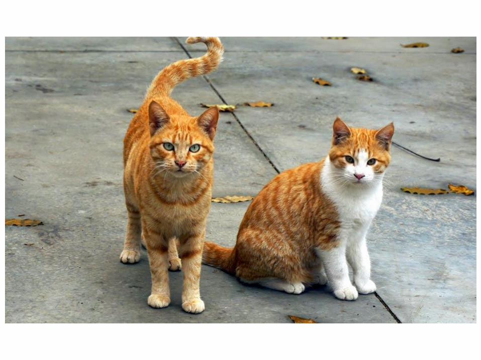
Story so far• Pattern classification tasks such as “does this picture contain a cat”, or
“does this recording include HELLO” are best performed by scanning for the target pattern
• Scanning an input with a network and combining the outcomes is equivalent to scanning with individual neurons
– First level neurons scan the input
– Higher-level neurons scan the “maps” formed by lower-level neurons
– A final “decision” unit or layer makes the final decision
• Deformations in the input can be handled by “max pooling”
• For 2-D (or higher-dimensional) scans, the structure is called a convnet
• For 1-D scan along time, it is called a Time-delay neural network
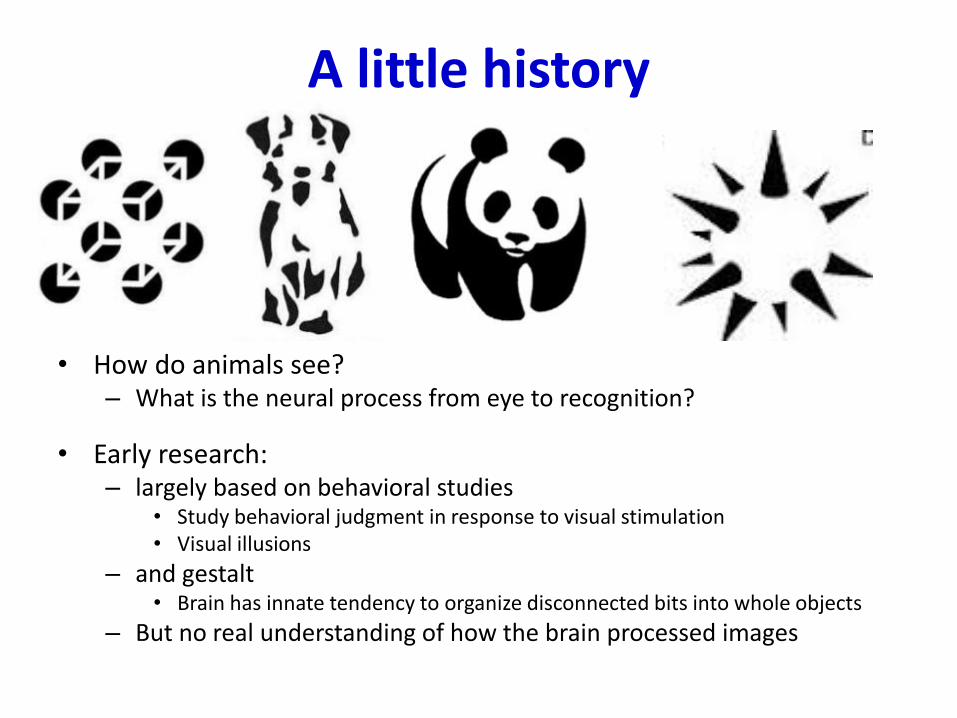
A little history
• How do animals see?– What is the neural process from eye to recognition?
• Early research: – largely based on behavioral studies
• Study behavioral judgment in response to visual stimulation• Visual illusions
– and gestalt• Brain has innate tendency to organize disconnected bits into whole objects
– But no real understanding of how the brain processed images
Hubel and Wiesel 1959
• First study on neural correlates of vision.
– “Receptive Fields in Cat Striate Cortex”
• “Striate Cortex”: Approximately equal to the V1 visual cortex– “Striate” – defined by structure, “V1” – functional definition
• 24 cats, anaesthetized, immobilized, on artificial respirators
– Anaesthetized with truth serum
– Electrodes into brain
• Do not report if cats survived experiment, but claim brain tissue was studied
Hubel and Wiesel 1959
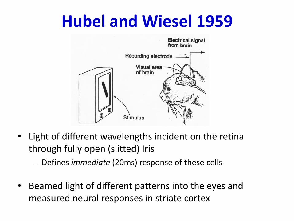
• Light of different wavelengths incident on the retina through fully open (slitted) Iris
– Defines immediate (20ms) response of these cells
• Beamed light of different patterns into the eyes and measured neural responses in striate cortex
Hubel and Wiesel 1959
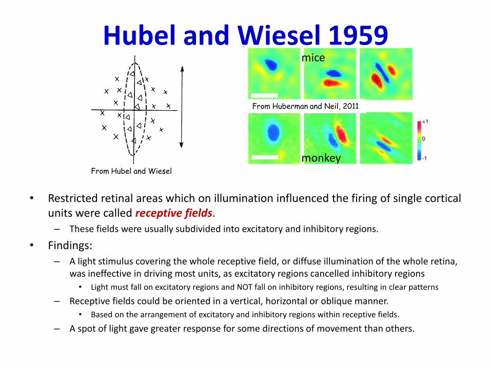
• Restricted retinal areas which on illumination influenced the firing of single cortical units were called receptive fields. – These fields were usually subdivided into excitatory and inhibitory regions.
• Findings:– A light stimulus covering the whole receptive field, or diffuse illumination of the whole retina,
was ineffective in driving most units, as excitatory regions cancelled inhibitory regions
• Light must fall on excitatory regions and NOT fall on inhibitory regions, resulting in clear patterns
– Receptive fields could be oriented in a vertical, horizontal or oblique manner.
• Based on the arrangement of excitatory and inhibitory regions within receptive fields.
– A spot of light gave greater response for some directions of movement than others.
mice
monkey
From Huberman and Neil, 2011
From Hubel and Wiesel
Hubel and Wiesel 59
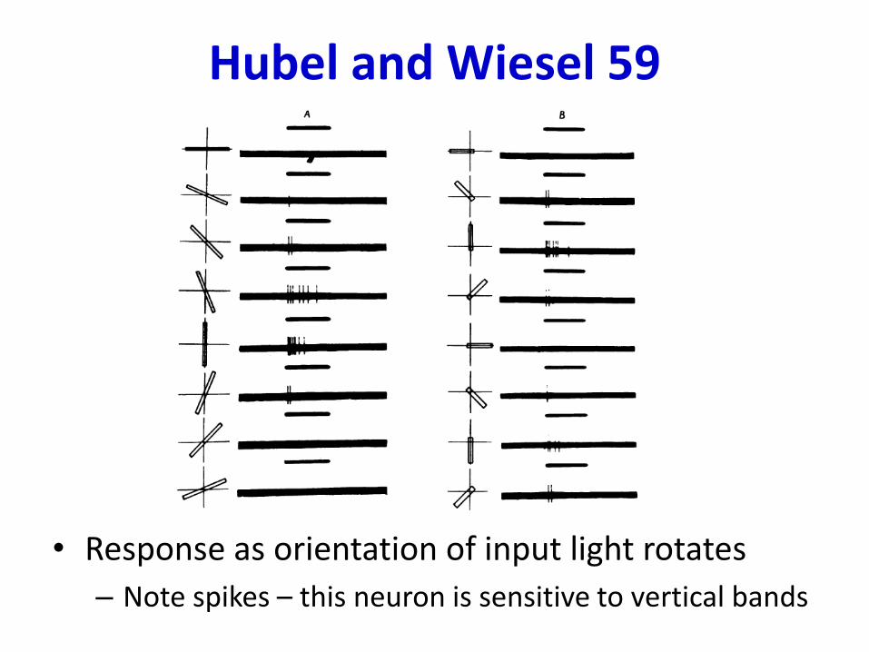
• Response as orientation of input light rotates
– Note spikes – this neuron is sensitive to vertical bands
Hubel and Wiesel
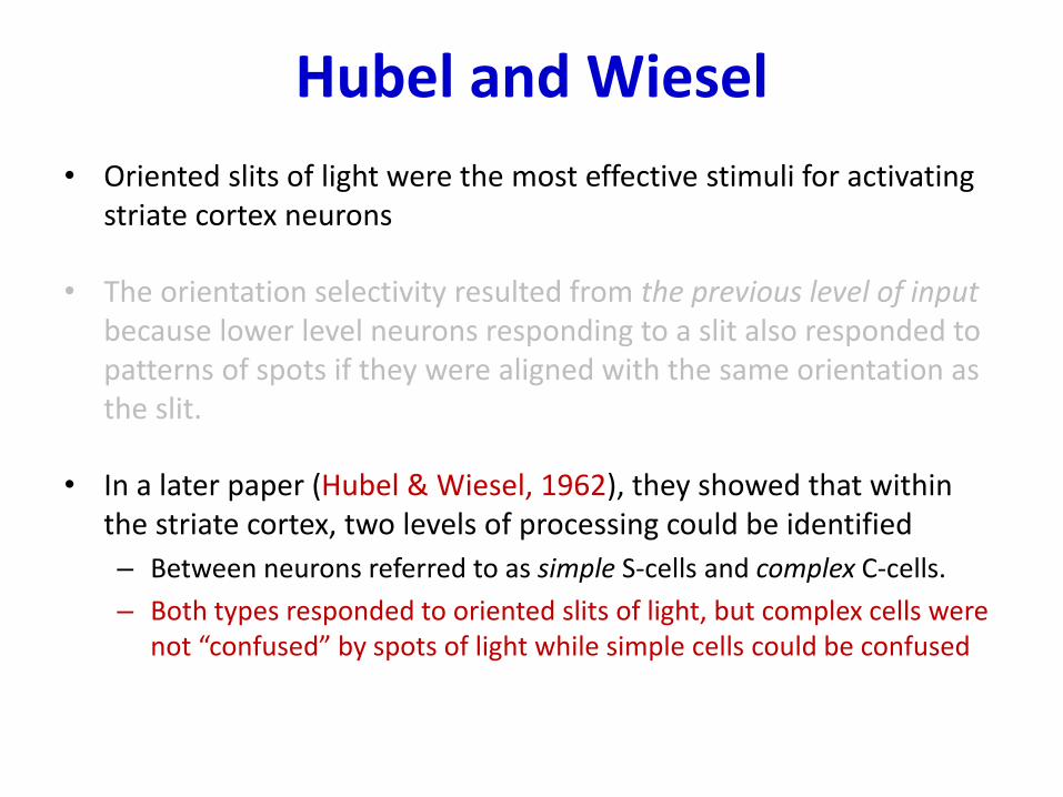
• Oriented slits of light were the most effective stimuli for activating striate cortex neurons
• The orientation selectivity resulted from the previous level of input because lower level neurons responding to a slit also responded to patterns of spots if they were aligned with the same orientation as the slit.
• In a later paper (Hubel & Wiesel, 1962), they showed that within the striate cortex, two levels of processing could be identified
– Between neurons referred to as simple S-cells and complex C-cells.
– Both types responded to oriented slits of light, but complex cells were not “confused” by spots of light while simple cells could be confused
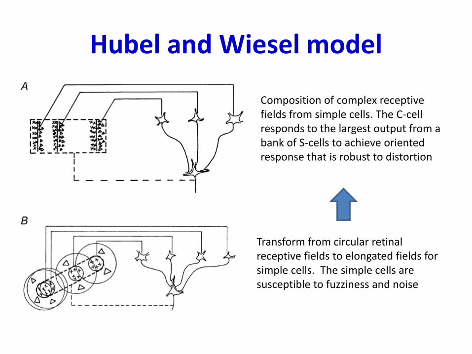
Hubel and Wiesel model
• ll
Transform from circular retinal receptive fields to elongated fields for simple cells. The simple cells are susceptible to fuzziness and noise
Composition of complex receptive fields from simple cells. The C-cell responds to the largest output from a bank of S-cells to achieve oriented response that is robust to distortion
Hubel and Wiesel
• Complex C-cells build from similarly oriented simple cells
– They “finetune” the response of the simple cell
• Show complex buildup – building more complex patterns by composing early neural responses
– Successive transformation through Simple-Complex combination layers
• Demonstrated more and more complex responses in later papers
– Later experiments were on waking macaque monkeys• Too horrible to recall
Hubel and Wiesel
• Complex cells build from similarly oriented simple cells– The “tune” the response of the simple cell and have similar response to the simple cell
• Show complex buildup – from point response of retina to oriented response of simple cells to cleaner response of complex cells
• Lead to more complex model of building more complex patterns by composing early neural responses– Successive transformations through Simple-Complex combination layers
• Demonstrated more and more complex responses in later papers• Experiments done by others were on waking monkeys
– Too horrible to recall
Adding insult to injury..
• “However, this model cannot accommodate the color, spatial frequency and many other features to which neurons are tuned. The exact organization of all these cortical columns within V1 remains a hot topic of current research.”
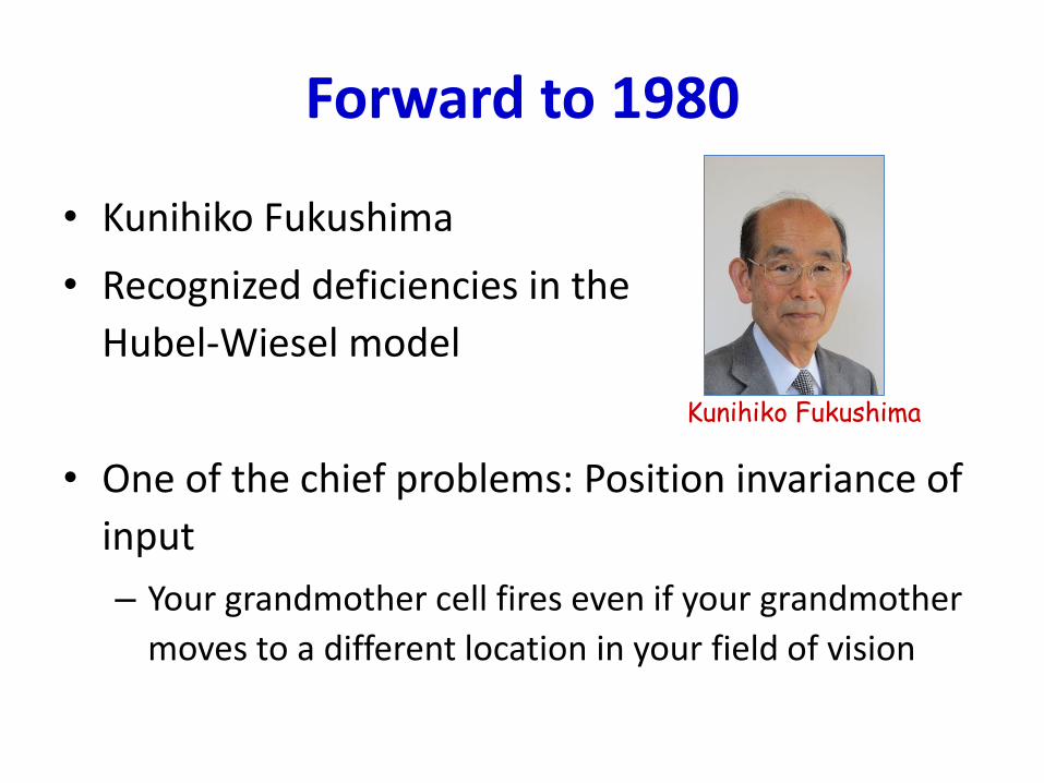
Forward to 1980
• Kunihiko Fukushima
• Recognized deficiencies in the
Hubel-Wiesel model
• One of the chief problems: Position invariance of
input
– Your grandmother cell fires even if your grandmother
moves to a different location in your field of vision
Kunihiko Fukushima
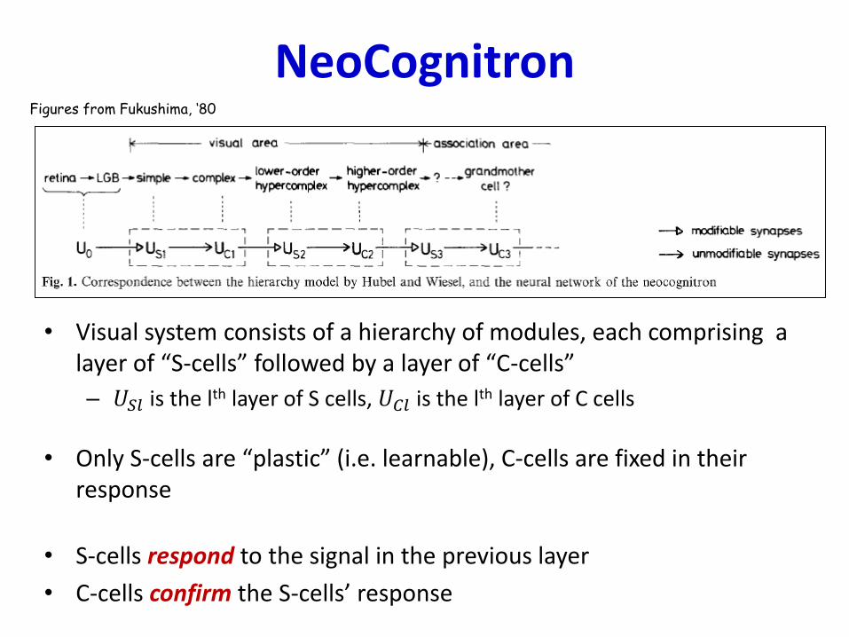
NeoCognitron
• Visual system consists of a hierarchy of modules, each comprising a layer of “S-cells” followed by a layer of “C-cells”
– 𝑈𝑆𝑙 is the lth layer of S cells, 𝑈𝐶𝑙 is the lth layer of C cells
• Only S-cells are “plastic” (i.e. learnable), C-cells are fixed in their response
• S-cells respond to the signal in the previous layer
• C-cells confirm the S-cells’ response
Figures from Fukushima, ‘80
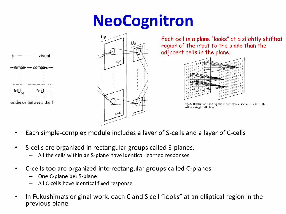
NeoCognitron
• Each simple-complex module includes a layer of S-cells and a layer of C-cells
• S-cells are organized in rectangular groups called S-planes. – All the cells within an S-plane have identical learned responses
• C-cells too are organized into rectangular groups called C-planes– One C-plane per S-plane– All C-cells have identical fixed response
• In Fukushima’s original work, each C and S cell “looks” at an elliptical region in the previous plane
Each cell in a plane “looks” at a slightly shiftedregion of the input to the plane than the adjacent cells in the plane.
NeoCognitron
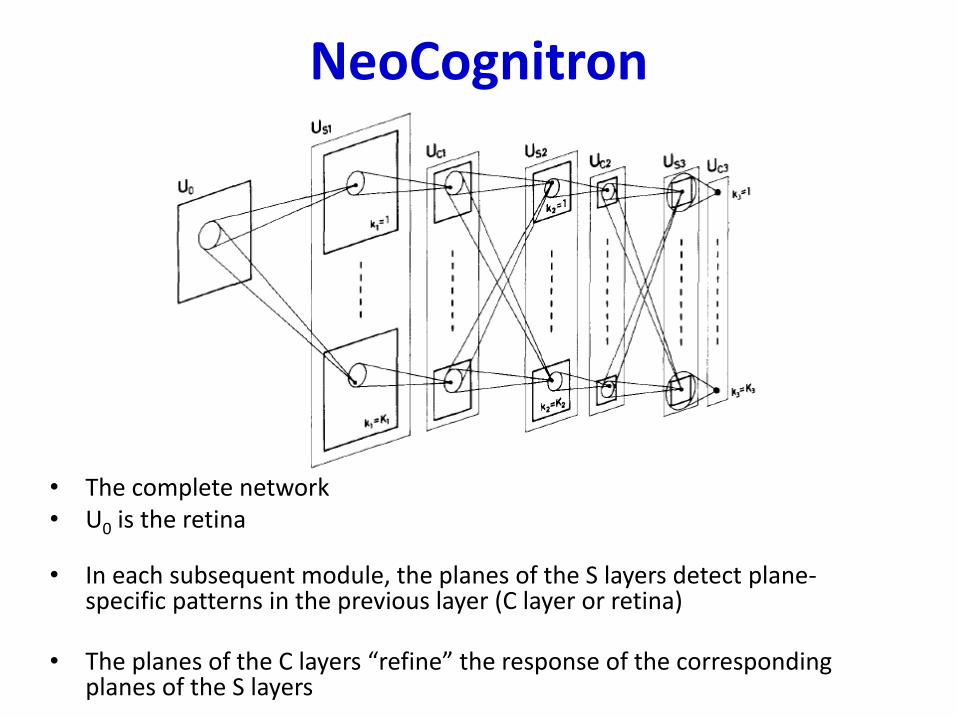
• The complete network• U0 is the retina
• In each subsequent module, the planes of the S layers detect plane-specific patterns in the previous layer (C layer or retina)
• The planes of the C layers “refine” the response of the corresponding planes of the S layers
Neocognitron
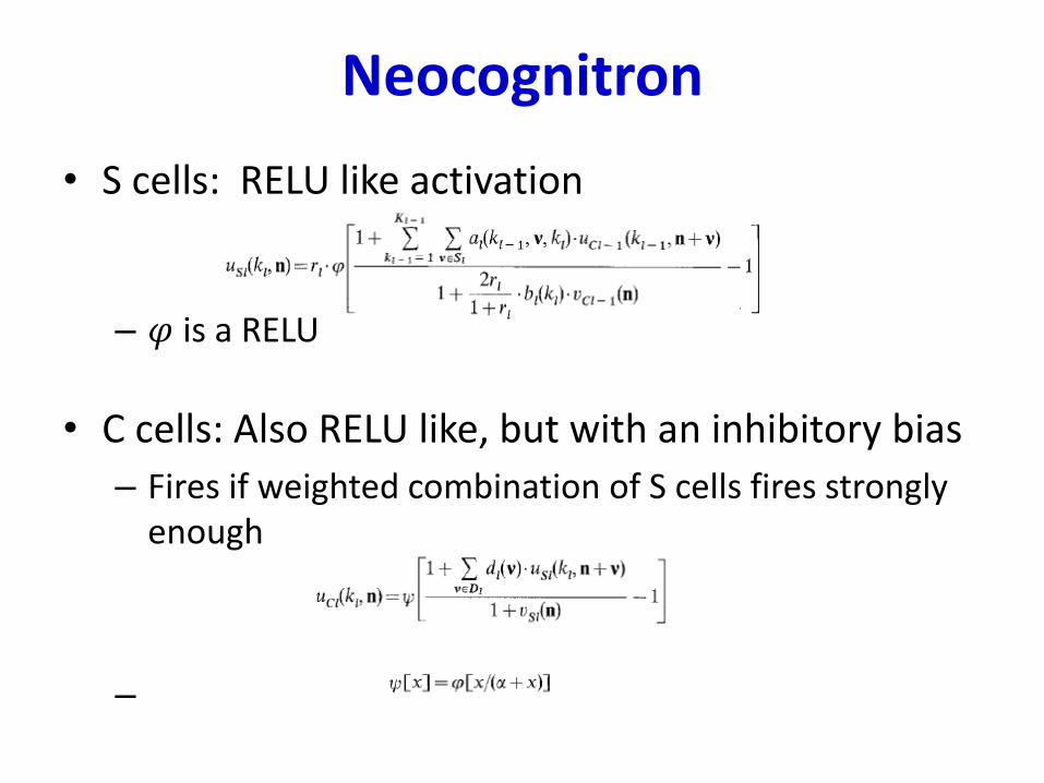
• S cells: RELU like activation
– 𝜑 is a RELU
• C cells: Also RELU like, but with an inhibitory bias
– Fires if weighted combination of S cells fires strongly enough
–
Neocognitron
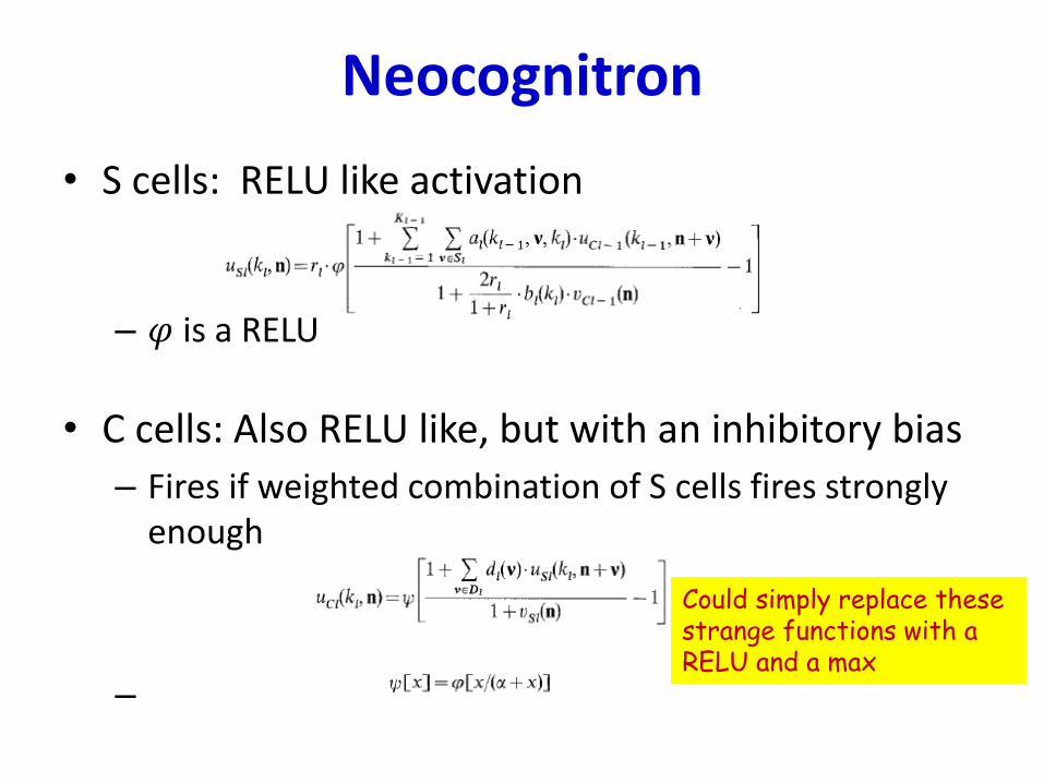
• S cells: RELU like activation
– 𝜑 is a RELU
• C cells: Also RELU like, but with an inhibitory bias
– Fires if weighted combination of S cells fires strongly enough
–
Could simply replace these strange functions with aRELU and a max
NeoCognitron
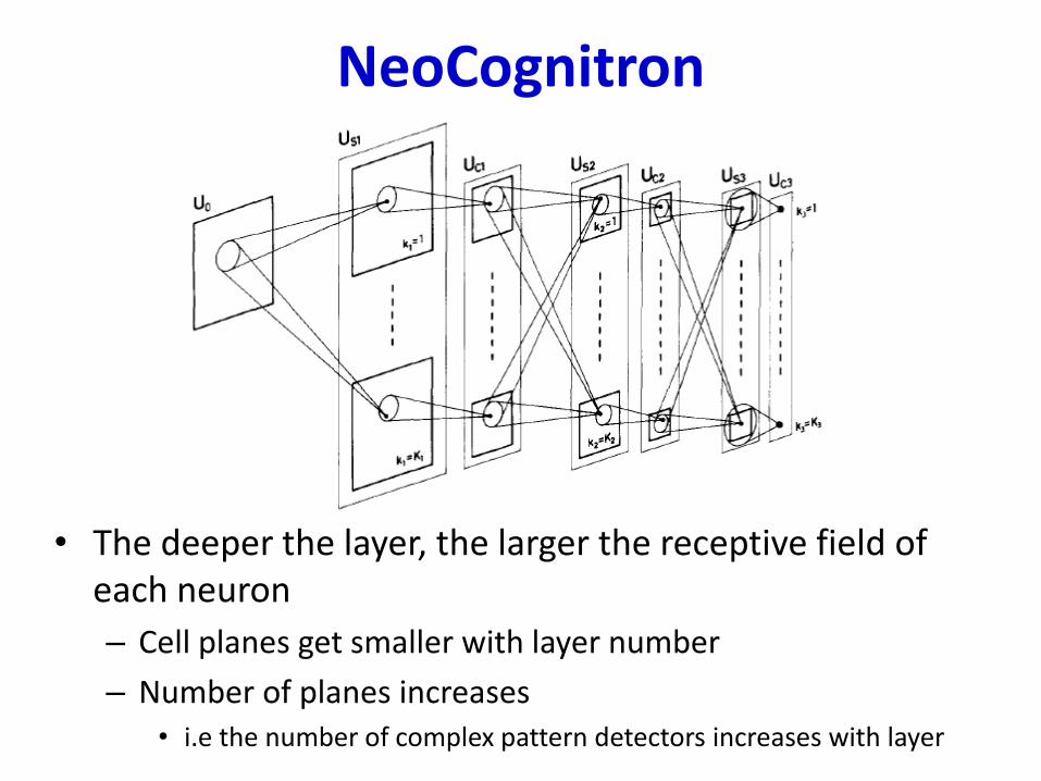
• The deeper the layer, the larger the receptive field of each neuron
– Cell planes get smaller with layer number
– Number of planes increases• i.e the number of complex pattern detectors increases with layer
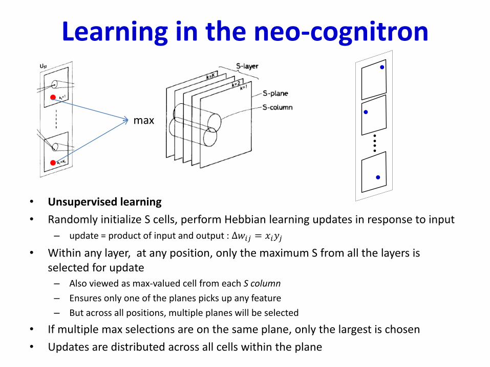
Learning in the neo-cognitron
• Unsupervised learning
• Randomly initialize S cells, perform Hebbian learning updates in response to input
– update = product of input and output : ∆𝑤𝑖𝑗 = 𝑥𝑖𝑦𝑗
• Within any layer, at any position, only the maximum S from all the layers is selected for update– Also viewed as max-valued cell from each S column
– Ensures only one of the planes picks up any feature
– But across all positions, multiple planes will be selected
• If multiple max selections are on the same plane, only the largest is chosen
• Updates are distributed across all cells within the plane
max
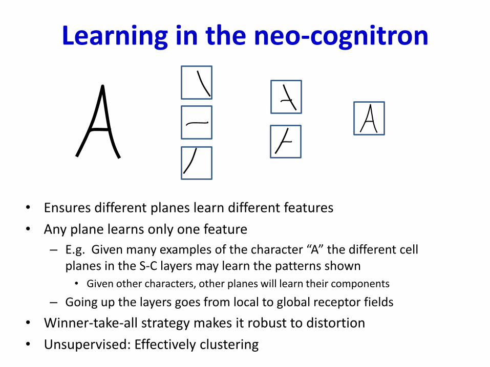
Learning in the neo-cognitron
• Ensures different planes learn different features
• Any plane learns only one feature
– E.g. Given many examples of the character “A” the different cell planes in the S-C layers may learn the patterns shown
• Given other characters, other planes will learn their components
– Going up the layers goes from local to global receptor fields
• Winner-take-all strategy makes it robust to distortion
• Unsupervised: Effectively clustering
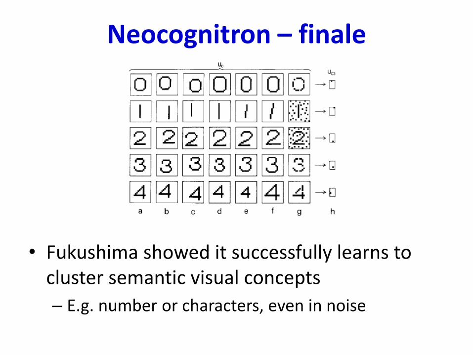
Neocognitron – finale
• Fukushima showed it successfully learns to cluster semantic visual concepts
– E.g. number or characters, even in noise
Adding Supervision
• The neocognitron is fully unsupervised
– Semantic labels are automatically learned
• Can we add external supervision?
• Various proposals:
– Temporal correlation: Homma, Atlas, Marks, 88
– TDNN: Lang, Waibel et. al., 1989, 90
• Convolutional neural networks: LeCun
Supervising the neocognitron
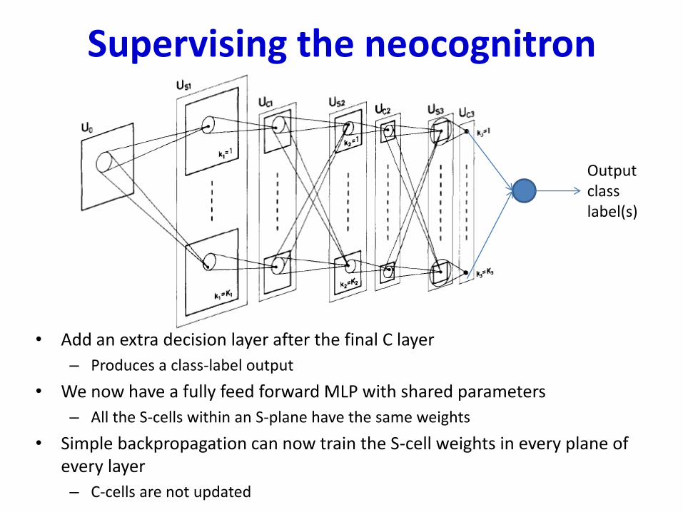
• Add an extra decision layer after the final C layer
– Produces a class-label output
• We now have a fully feed forward MLP with shared parameters
– All the S-cells within an S-plane have the same weights
• Simple backpropagation can now train the S-cell weights in every plane of every layer
– C-cells are not updated
Outputclass label(s)
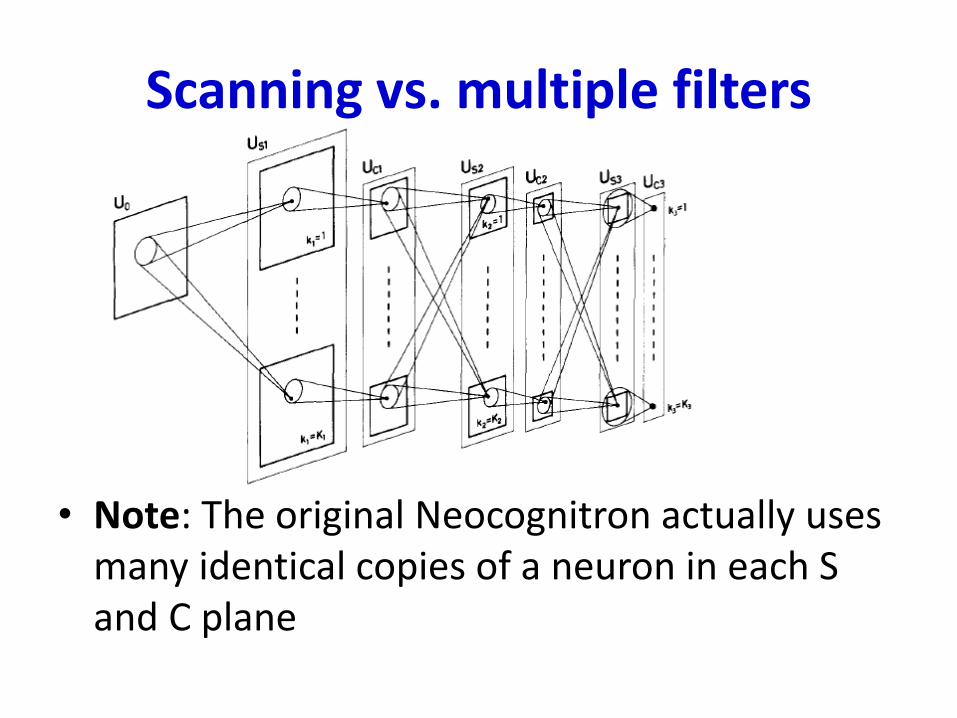
Scanning vs. multiple filters
• Note: The original Neocognitron actually uses many identical copies of a neuron in each S and C plane
Supervising the neocognitron
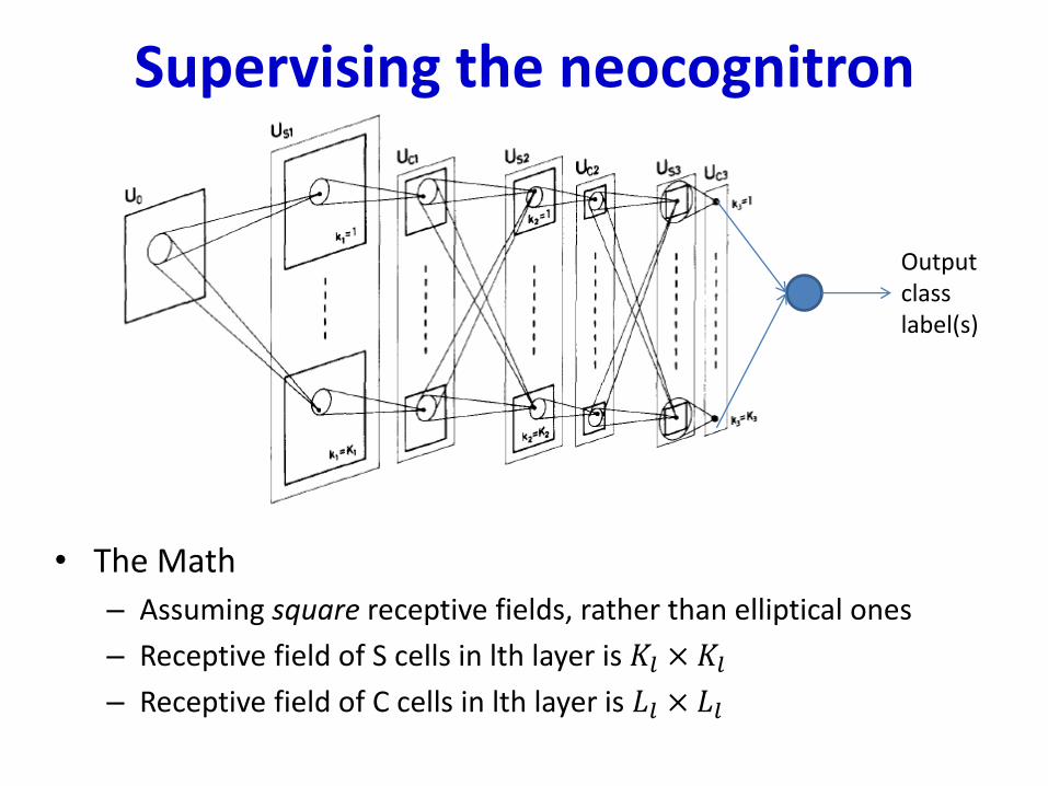
• The Math
– Assuming square receptive fields, rather than elliptical ones
– Receptive field of S cells in lth layer is 𝐾𝑙 × 𝐾𝑙– Receptive field of C cells in lth layer is 𝐿𝑙 × 𝐿𝑙
Outputclass label(s)
Supervising the neocognitron
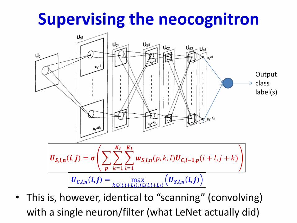
• This is, however, identical to “scanning” (convolving)
with a single neuron/filter (what LeNet actually did)
Outputclass label(s)
𝑼𝑺,𝒍,𝒏 𝒊, 𝒋 = 𝝈
𝒑
𝑘=1
𝑲𝒍
𝑙=1
𝑲𝒍
𝒘𝑺,𝒍,𝒏(𝑝, 𝑘, 𝑙)𝑼𝑪,𝒍−𝟏,𝒑(𝑖 + 𝑙, 𝑗 + 𝑘)
𝑼𝑪,𝒍,𝒏 𝒊, 𝒋 = max𝑘∈ 𝑖,𝑖+𝐿𝑙 ,𝑗∈(𝑙,𝑙+𝐿𝑙)
𝑼𝑺,𝒍,𝒏 𝒊, 𝒋
Convolutional Neural Networks
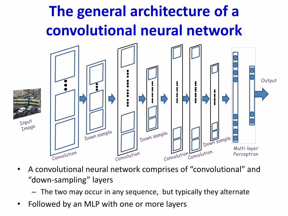
The general architecture of a convolutional neural network
• A convolutional neural network comprises of “convolutional” and “down-sampling” layers
– The two may occur in any sequence, but typically they alternate
• Followed by an MLP with one or more layers
Multi-layerPerceptron
Output
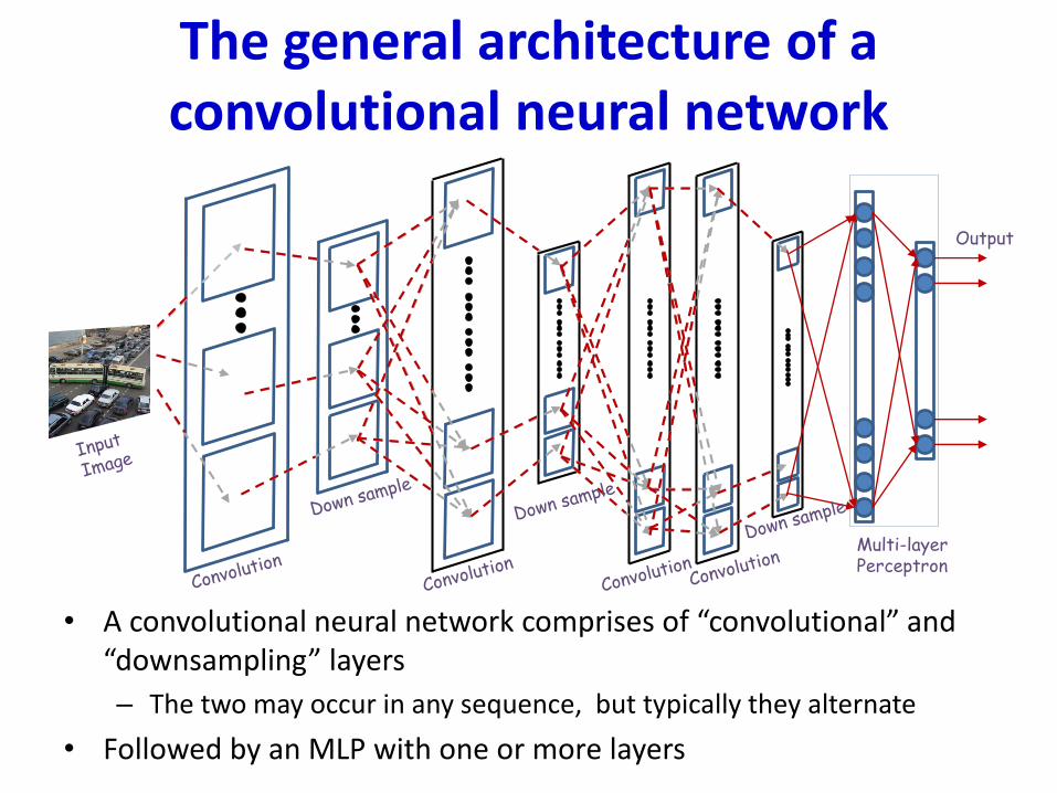
The general architecture of a convolutional neural network
• A convolutional neural network comprises of “convolutional” and “downsampling” layers
– The two may occur in any sequence, but typically they alternate
• Followed by an MLP with one or more layers
Multi-layerPerceptron
Output
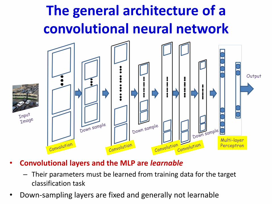
The general architecture of a convolutional neural network
• Convolutional layers and the MLP are learnable
– Their parameters must be learned from training data for the target classification task
• Down-sampling layers are fixed and generally not learnable
Multi-layerPerceptron
Output
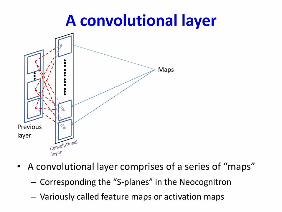
A convolutional layer
• A convolutional layer comprises of a series of “maps”
– Corresponding the “S-planes” in the Neocognitron
– Variously called feature maps or activation maps
Maps
Previouslayer
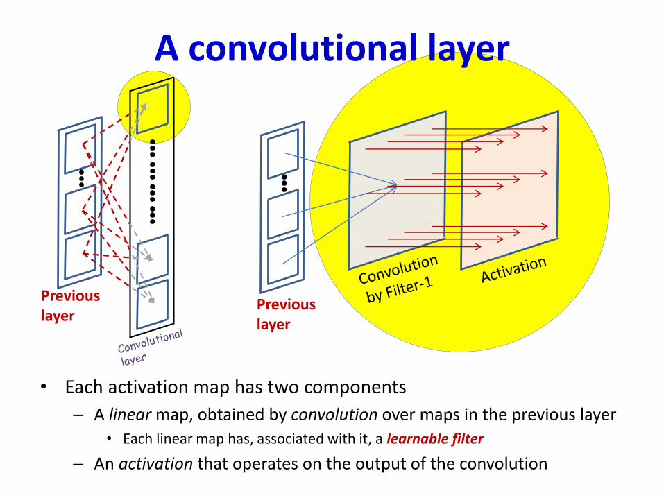
A convolutional layer
• Each activation map has two components
– A linear map, obtained by convolution over maps in the previous layer
• Each linear map has, associated with it, a learnable filter
– An activation that operates on the output of the convolution
Previouslayer
Previouslayer
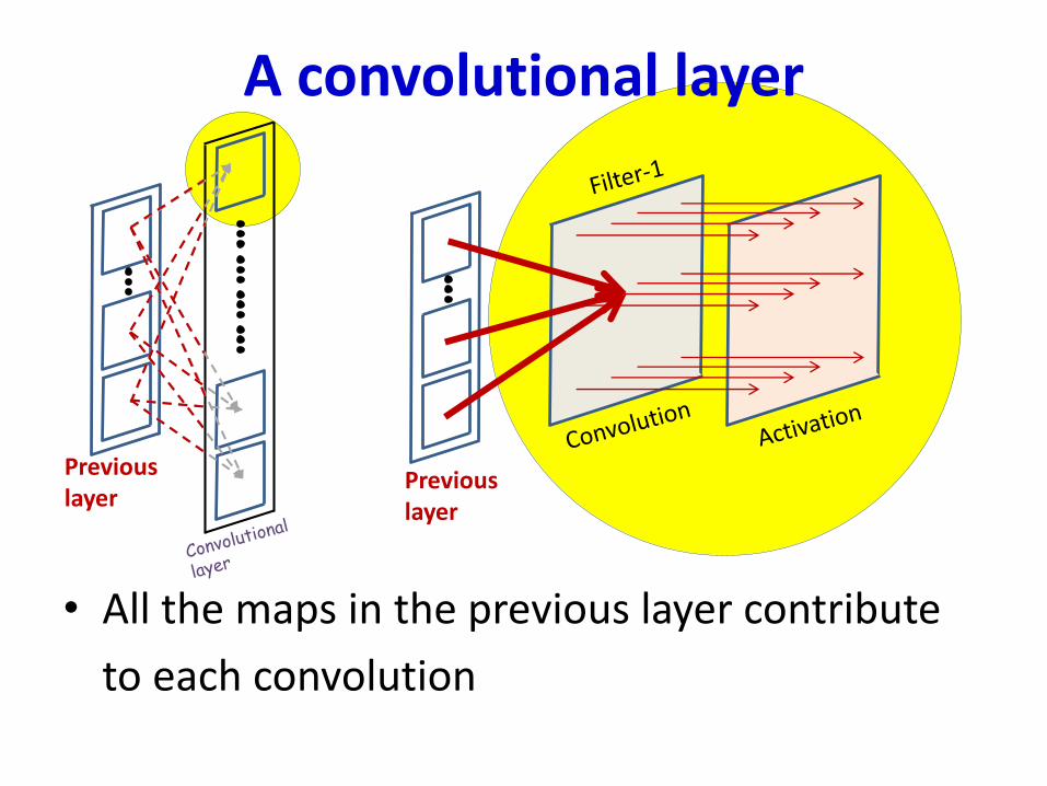
A convolutional layer
• All the maps in the previous layer contribute
to each convolution
Previouslayer
Previouslayer
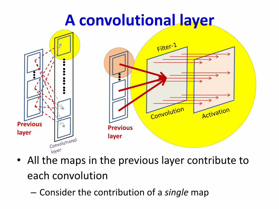
A convolutional layer
• All the maps in the previous layer contribute to
each convolution
– Consider the contribution of a single map
Previouslayer
Previouslayer
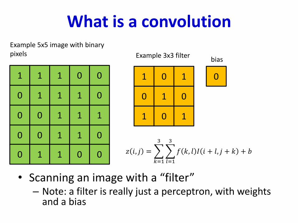
What is a convolution
• Scanning an image with a “filter”– Note: a filter is really just a perceptron, with weights
and a bias
1 1 1 0 0
0 1 1 1 0
1 1 10 0
0 0 01 1
0 1 01 0
Example 5x5 image with binarypixels
1 0 1
0 1 0
11 0
0
Example 3x3 filter
𝑧 𝑖, 𝑗 =
𝑘=1
3
𝑙=1
3
𝑓 𝑘, 𝑙 𝐼 𝑖 + 𝑙, 𝑗 + 𝑘 + 𝑏
bias
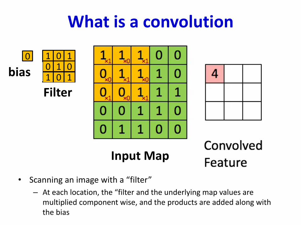
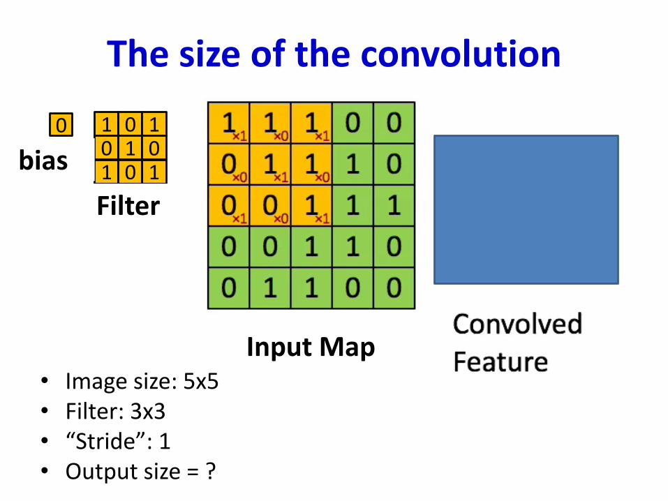
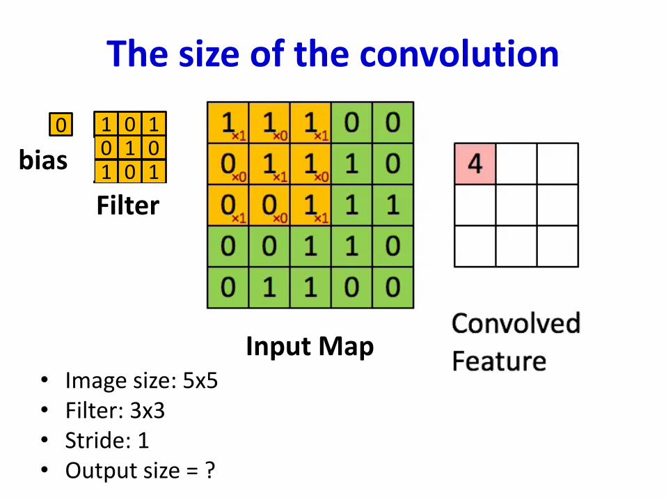
What is a convolution
• Scanning an image with a “filter”
– At each location, the “filter and the underlying map values are multiplied component wise, and the products are added along with the bias
1 0 10 1 0
11 0
Input Map
Filter
0
bias
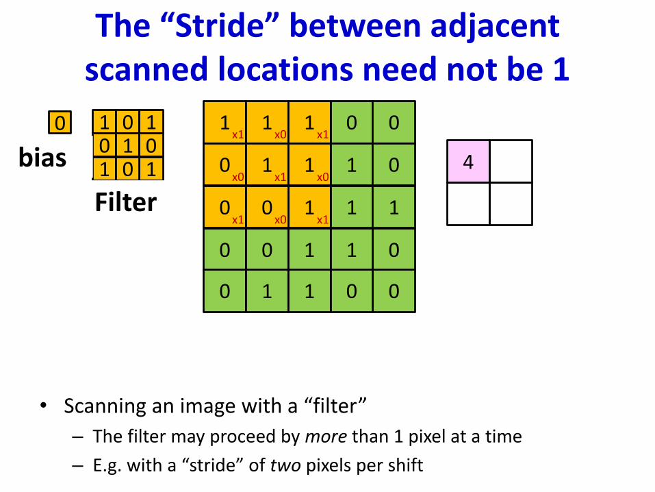
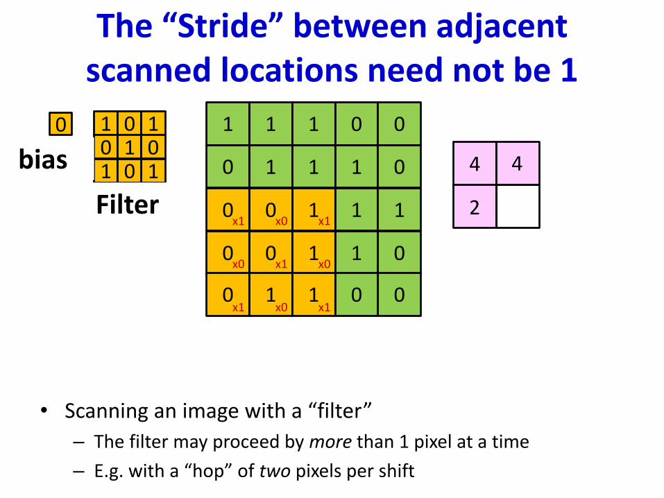
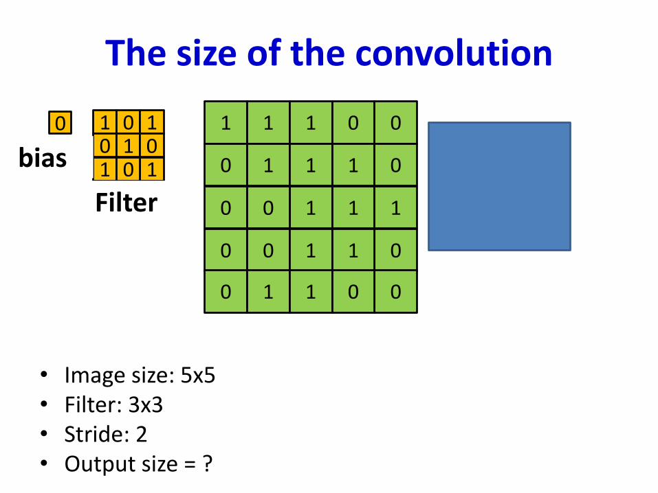
The “Stride” between adjacent scanned locations need not be 1
• Scanning an image with a “filter”
– The filter may proceed by more than 1 pixel at a time
– E.g. with a “stride” of two pixels per shift
1 1 1 0 0
0 1 1 1 0
1 1 10 0
0 0 01 1
0 1 01 0
4
x1 x0 x1
x0 x1 x0
x1x1 x0
1 0 10 1 0
11 0
Filter
0
bias
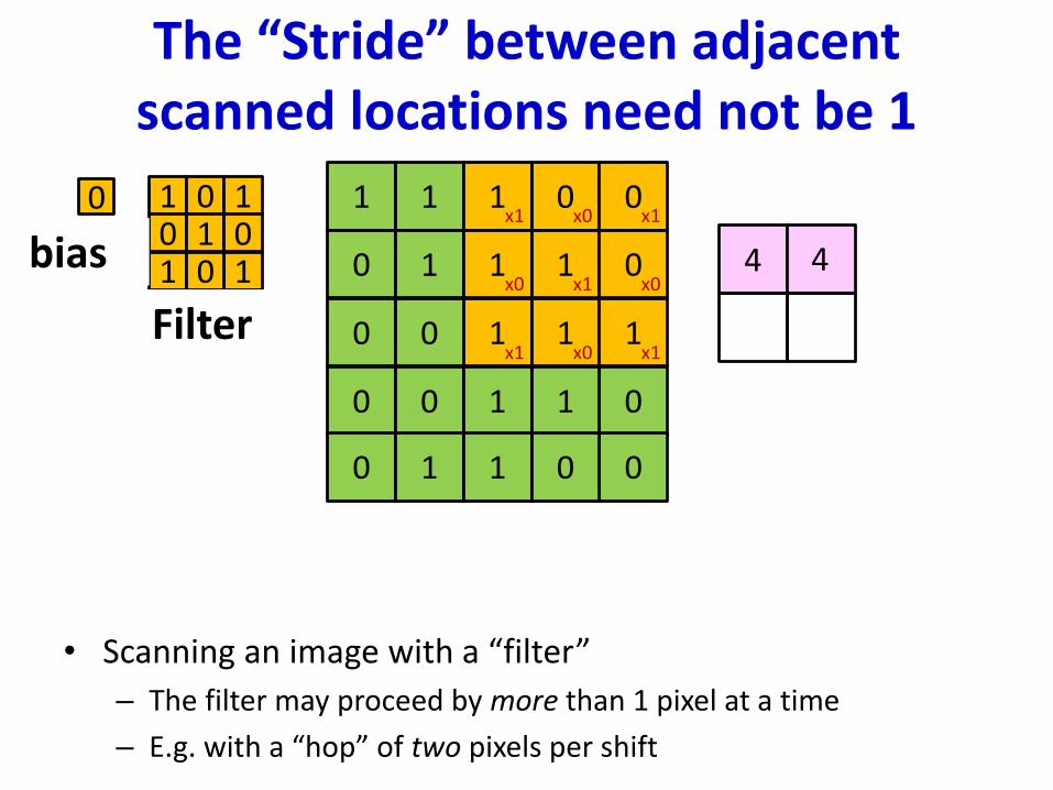
The “Stride” between adjacent scanned locations need not be 1
1 1 1 0 0
0 1 1 1 0
1 1 10 0
0 0 01 1
0 1 01 0
x1 x0 x1
x0 x1 x0
x1x1 x0
1 0 10 1 0
11 0
Filter
0
bias
• Scanning an image with a “filter”
– The filter may proceed by more than 1 pixel at a time
– E.g. with a “hop” of two pixels per shift
4 4
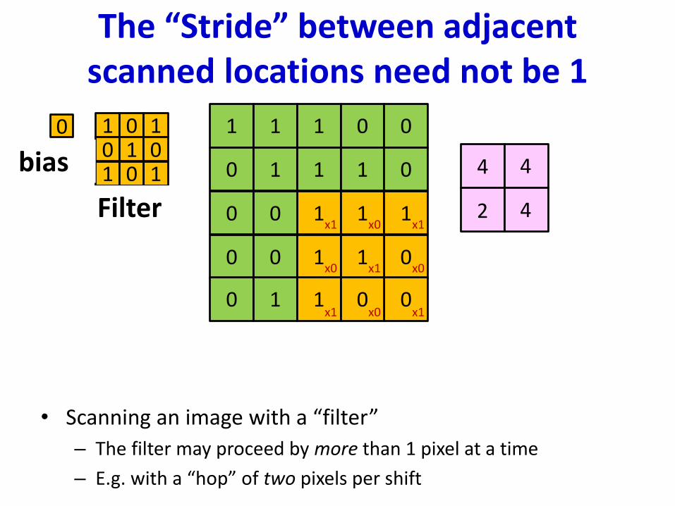
2
The “Stride” between adjacent scanned locations need not be 1
1 1 1 0 0
0 1 1 1 0
1 1 10 0
0 0 01 1
0 1 01 0
x1 x0 x1
x0 x1 x0
x1x1 x0
1 0 10 1 0
11 0
Filter
0
bias
• Scanning an image with a “filter”
– The filter may proceed by more than 1 pixel at a time
– E.g. with a “hop” of two pixels per shift
4 4
2 4
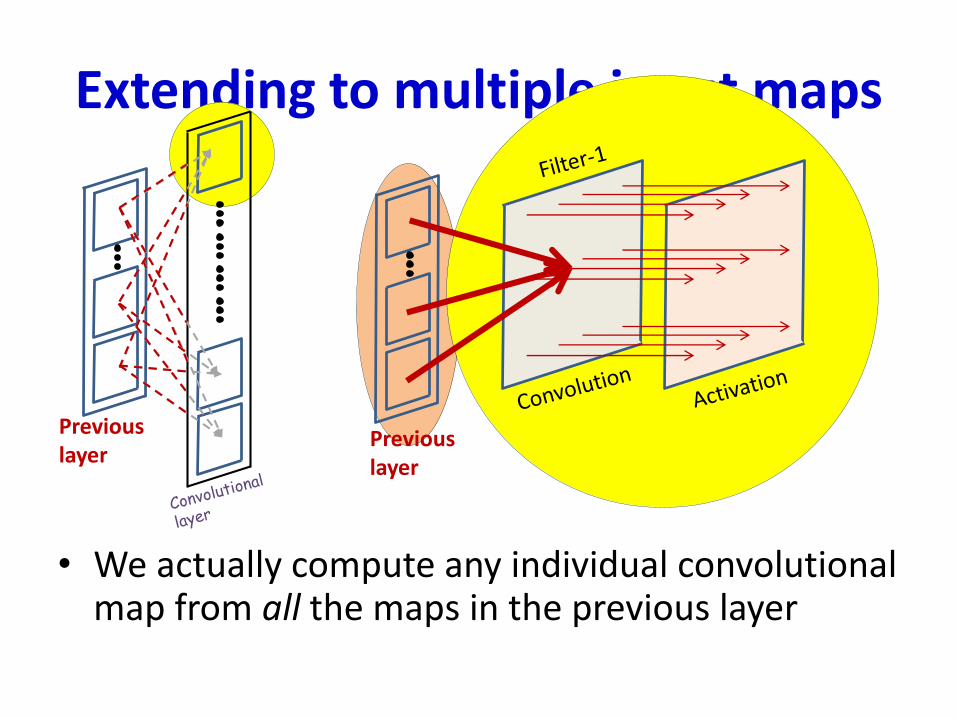
Extending to multiple input maps
• We actually compute any individual convolutional map from all the maps in the previous layer
Previouslayer
Previouslayer
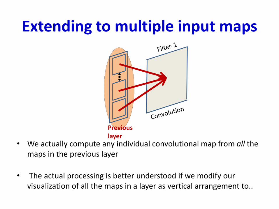
Extending to multiple input maps
• We actually compute any individual convolutional map from all the maps in the previous layer
• The actual processing is better understood if we modify our visualization of all the maps in a layer as vertical arrangement to..
Previouslayer
Extending to multiple input maps
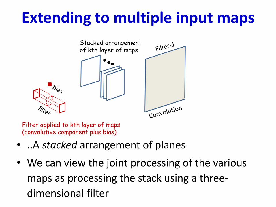
• ..A stacked arrangement of planes
• We can view the joint processing of the various
maps as processing the stack using a three-
dimensional filter
Stacked arrangementof kth layer of maps
Filter applied to kth layer of maps(convolutive component plus bias)
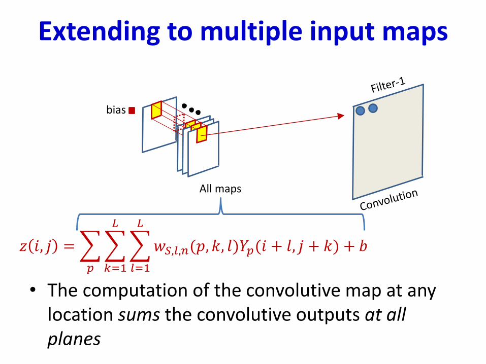
Extending to multiple input maps
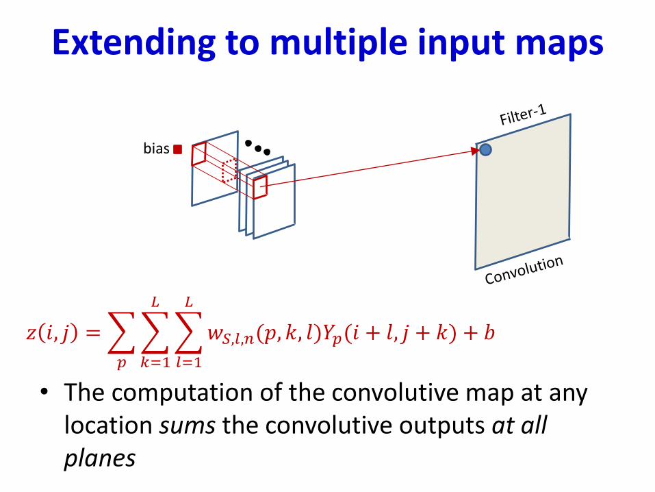
• The computation of the convolutive map at any location sums the convolutive outputs at all planes
𝑧 𝑖, 𝑗 =
𝑝
𝑘=1
𝐿
𝑙=1
𝐿
𝑤𝑆,𝑙,𝑛(𝑝, 𝑘, 𝑙)𝑌𝑝(𝑖 + 𝑙, 𝑗 + 𝑘) + 𝑏
bias
Extending to multiple input maps
• The computation of the convolutive map at any location sums the convolutive outputs at all planes
𝑧 𝑖, 𝑗 =
𝑝
𝑘=1
𝐿
𝑙=1
𝐿
𝑤𝑆,𝑙,𝑛(𝑝, 𝑘, 𝑙)𝑌𝑝(𝑖 + 𝑙, 𝑗 + 𝑘) + 𝑏
One map
bias
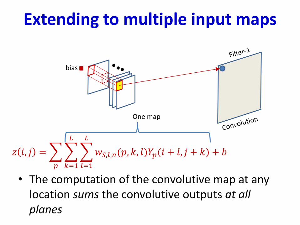
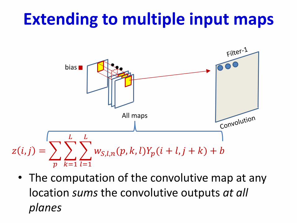
Extending to multiple input maps
• The computation of the convolutive map at any location sums the convolutive outputs at all planes
𝑧 𝑖, 𝑗 =
𝑝
𝑘=1
𝐿
𝑙=1
𝐿
𝑤𝑆,𝑙,𝑛(𝑝, 𝑘, 𝑙)𝑌𝑝(𝑖 + 𝑙, 𝑗 + 𝑘) + 𝑏
All maps
bias
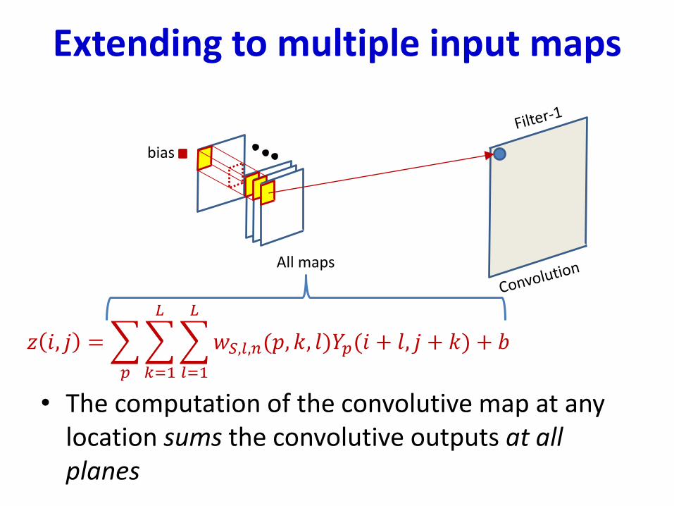
Extending to multiple input maps
• The computation of the convolutive map at any location sums the convolutive outputs at all planes
𝑧 𝑖, 𝑗 =
𝑝
𝑘=1
𝐿
𝑙=1
𝐿
𝑤𝑆,𝑙,𝑛(𝑝, 𝑘, 𝑙)𝑌𝑝(𝑖 + 𝑙, 𝑗 + 𝑘) + 𝑏
All maps
bias
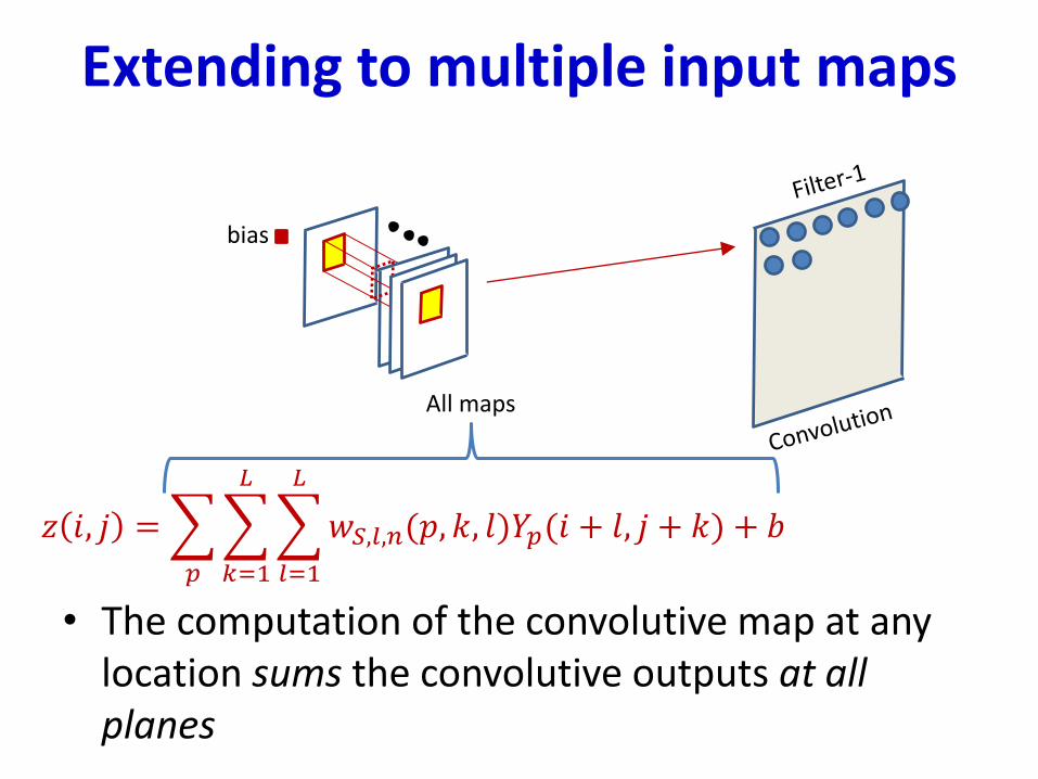
Extending to multiple input maps
• The computation of the convolutive map at any location sums the convolutive outputs at all planes
𝑧 𝑖, 𝑗 =
𝑝
𝑘=1
𝐿
𝑙=1
𝐿
𝑤𝑆,𝑙,𝑛(𝑝, 𝑘, 𝑙)𝑌𝑝(𝑖 + 𝑙, 𝑗 + 𝑘) + 𝑏
All maps
bias

Extending to multiple input maps
• The computation of the convolutive map at any location sums the convolutive outputs at all planes
𝑧 𝑖, 𝑗 =
𝑝
𝑘=1
𝐿
𝑙=1
𝐿
𝑤𝑆,𝑙,𝑛(𝑝, 𝑘, 𝑙)𝑌𝑝(𝑖 + 𝑙, 𝑗 + 𝑘) + 𝑏
All maps
bias
Extending to multiple input maps
• The computation of the convolutive map at any location sums the convolutive outputs at all planes
𝑧 𝑖, 𝑗 =
𝑝
𝑘=1
𝐿
𝑙=1
𝐿
𝑤𝑆,𝑙,𝑛(𝑝, 𝑘, 𝑙)𝑌𝑝(𝑖 + 𝑙, 𝑗 + 𝑘) + 𝑏
All maps
bias
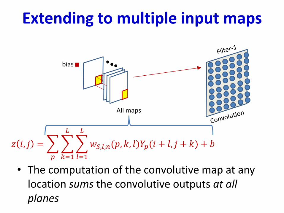
Extending to multiple input maps
• The computation of the convolutive map at any location sums the convolutive outputs at all planes
𝑧 𝑖, 𝑗 =
𝑝
𝑘=1
𝐿
𝑙=1
𝐿
𝑤𝑆,𝑙,𝑛(𝑝, 𝑘, 𝑙)𝑌𝑝(𝑖 + 𝑙, 𝑗 + 𝑘) + 𝑏
All maps
bias
The size of the convolution
1 0 10 1 0
11 0
Input Map
Filter
0
bias
• Image size: 5x5• Filter: 3x3• “Stride”: 1• Output size = ?
The size of the convolution
1 0 10 1 0
11 0
Input Map
Filter
0
bias
• Image size: 5x5• Filter: 3x3• Stride: 1• Output size = ?
The size of the convolution
• Image size: 5x5• Filter: 3x3• Stride: 2• Output size = ?
1 1 1 0 0
0 1 1 1 0
1 1 10 0
0 0 01 1
0 1 01 0
1 0 10 1 0
11 0
Filter
0
bias 4 4
2 4
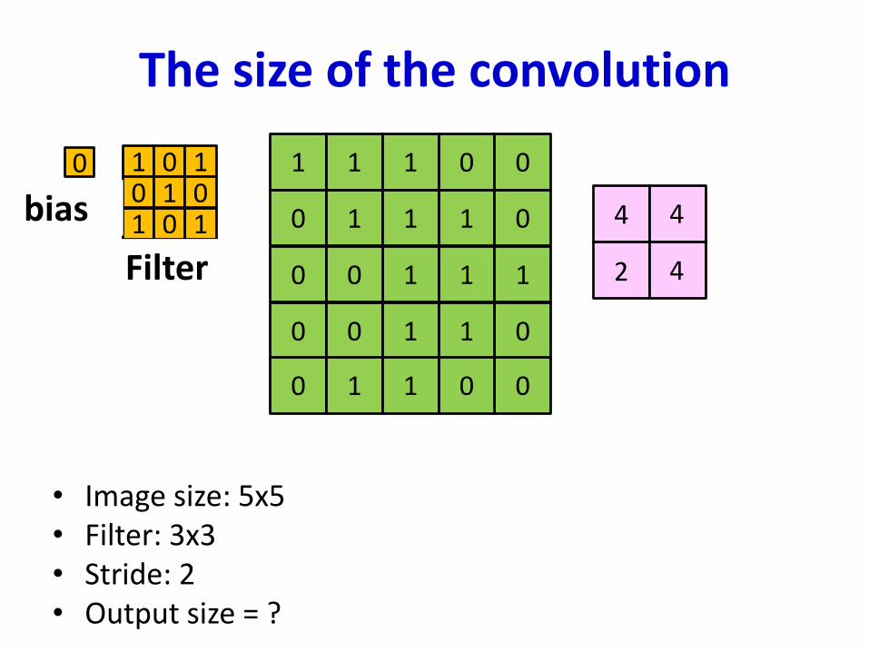
The size of the convolution
• Image size: 5x5• Filter: 3x3• Stride: 2• Output size = ?
1 1 1 0 0
0 1 1 1 0
1 1 10 0
0 0 01 1
0 1 01 0
1 0 10 1 0
11 0
Filter
0
bias 4 4
2 4
The size of the convolution
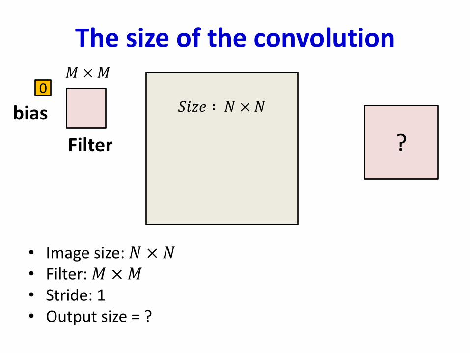
• Image size: 𝑁 × 𝑁• Filter: 𝑀 ×𝑀• Stride: 1• Output size = ?
1 1 1 0 0
0 1 1 1 0
1 1 10 0
0 0 01 1
0 1 01 0
Filter
0
bias 𝑆𝑖𝑧𝑒 ∶ 𝑁 × 𝑁
𝑀 ×𝑀
?

The size of the convolution
• Image size: 𝑁 × 𝑁• Filter: 𝑀 ×𝑀• Stride: 𝑆• Output size = ?
1 1 1 0 0
0 1 1 1 0
1 1 10 0
0 0 01 1
0 1 01 0
Filter
0
bias 𝑆𝑖𝑧𝑒 ∶ 𝑁 × 𝑁
𝑀 ×𝑀
?
The size of the convolution
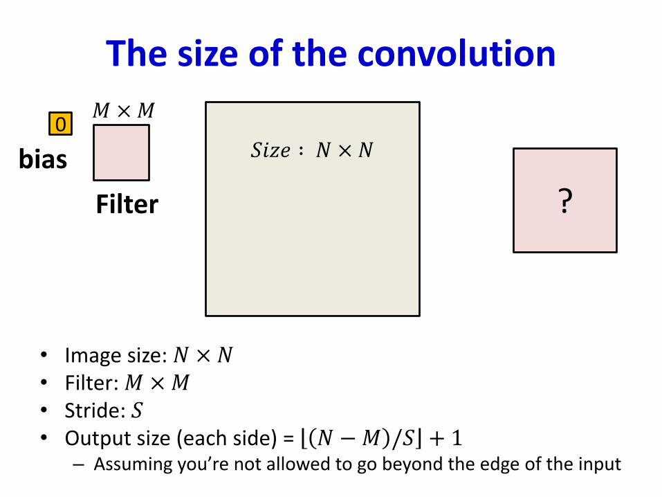
• Image size: 𝑁 × 𝑁• Filter: 𝑀 ×𝑀• Stride: 𝑆• Output size (each side) = 𝑁 −𝑀 /𝑆 + 1
– Assuming you’re not allowed to go beyond the edge of the input
1 1 1 0 0
0 1 1 1 0
1 1 10 0
0 0 01 1
0 1 01 0
Filter
0
bias 𝑆𝑖𝑧𝑒 ∶ 𝑁 × 𝑁
𝑀 ×𝑀
?
Convolution Size
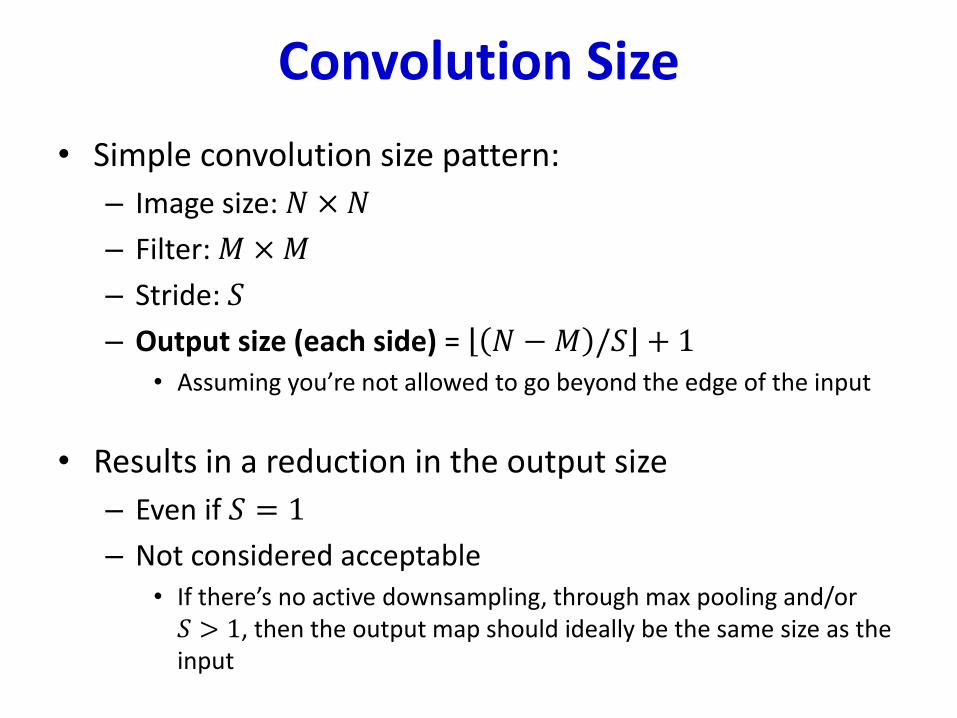
• Simple convolution size pattern:
– Image size: 𝑁 × 𝑁
– Filter: 𝑀 ×𝑀
– Stride: 𝑆
– Output size (each side) = 𝑁 −𝑀 /𝑆 + 1• Assuming you’re not allowed to go beyond the edge of the input
• Results in a reduction in the output size
– Even if 𝑆 = 1
– Not considered acceptable• If there’s no active downsampling, through max pooling and/or 𝑆 > 1, then the output map should ideally be the same size as the input
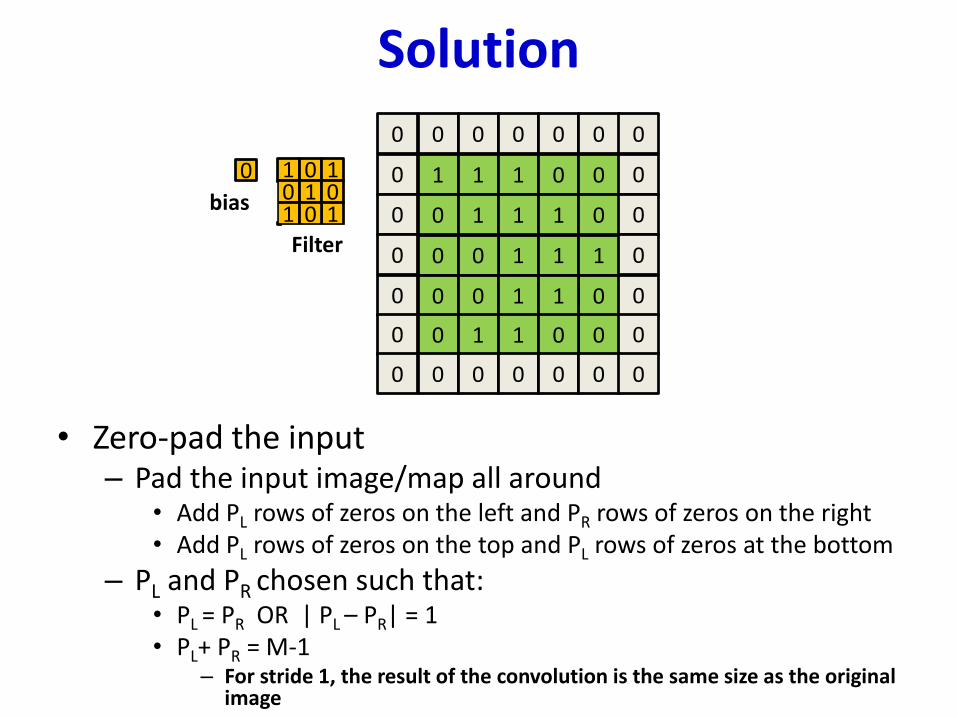
Solution
• Zero-pad the input– Pad the input image/map all around
• Add PL rows of zeros on the left and PR rows of zeros on the right• Add PL rows of zeros on the top and PL rows of zeros at the bottom
– PL and PR chosen such that:• PL = PR OR | PL – PR| = 1• PL+ PR = M-1
– For stride 1, the result of the convolution is the same size as the original image
1 1 1 0 0
0 1 1 1 0
1 1 10 0
0 0 01 1
0 1 01 0
1 0 10 1 0
11 0
Filter
0
bias0
0
0
0
0
0
0
0
0
0
0 0 0 0 00 0
0 0 0 0 00 0
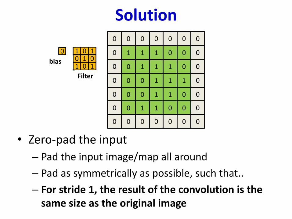
Solution
• Zero-pad the input
– Pad the input image/map all around
– Pad as symmetrically as possible, such that..
– For stride 1, the result of the convolution is the same size as the original image
1 1 1 0 0
0 1 1 1 0
1 1 10 0
0 0 01 1
0 1 01 0
1 0 10 1 0
11 0
Filter
0
bias0
0
0
0
0
0
0
0
0
0
0 0 0 0 00 0
0 0 0 0 00 0
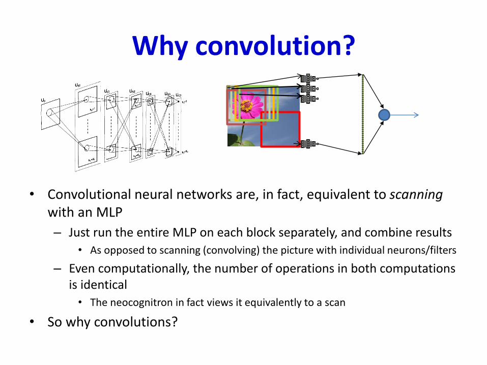
Why convolution?
• Convolutional neural networks are, in fact, equivalent to scanning with an MLP
– Just run the entire MLP on each block separately, and combine results
• As opposed to scanning (convolving) the picture with individual neurons/filters
– Even computationally, the number of operations in both computations is identical
• The neocognitron in fact views it equivalently to a scan
• So why convolutions?
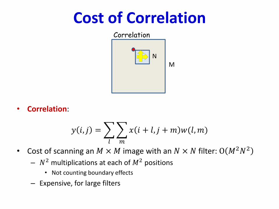
Cost of Correlation
• Correlation:
𝑦 𝑖, 𝑗 =
𝑙
𝑚
𝑥 𝑖 + 𝑙, 𝑗 + 𝑚 𝑤(𝑙,𝑚)
• Cost of scanning an 𝑀 ×𝑀 image with an 𝑁 × 𝑁 filter: O 𝑀2𝑁2
– 𝑁2 multiplications at each of 𝑀2 positions
• Not counting boundary effects
– Expensive, for large filters
Correlation
MN
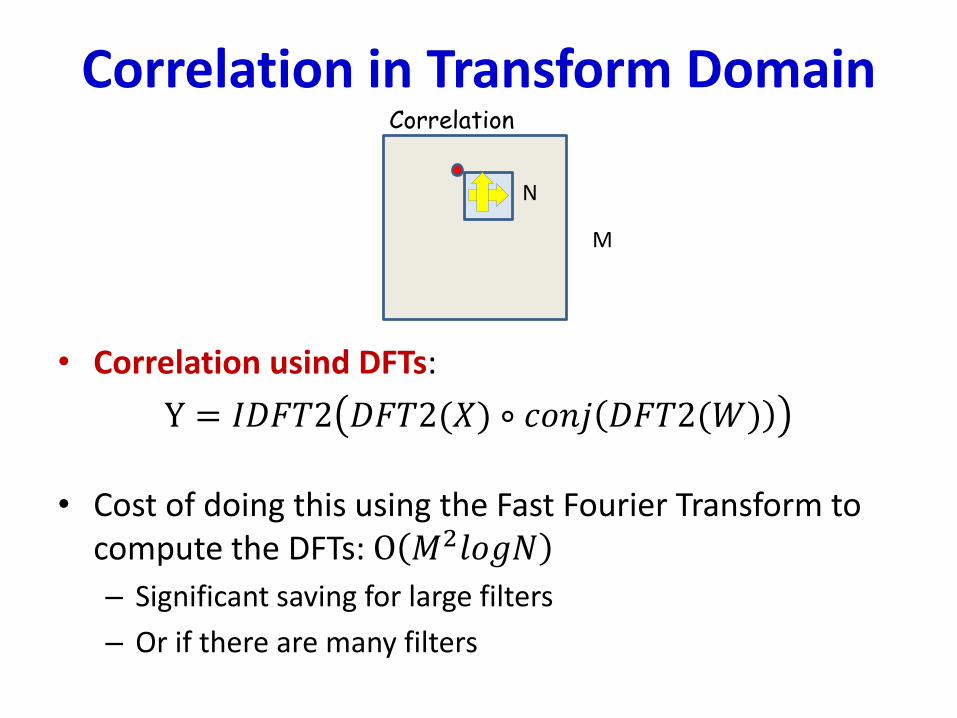
Correlation in Transform Domain
• Correlation usind DFTs:
Y = 𝐼𝐷𝐹𝑇2 𝐷𝐹𝑇2(𝑋) ∘ 𝑐𝑜𝑛𝑗 𝐷𝐹𝑇2(𝑊)
• Cost of doing this using the Fast Fourier Transform to compute the DFTs: O 𝑀2𝑙𝑜𝑔𝑁
– Significant saving for large filters
– Or if there are many filters
Correlation
M
N
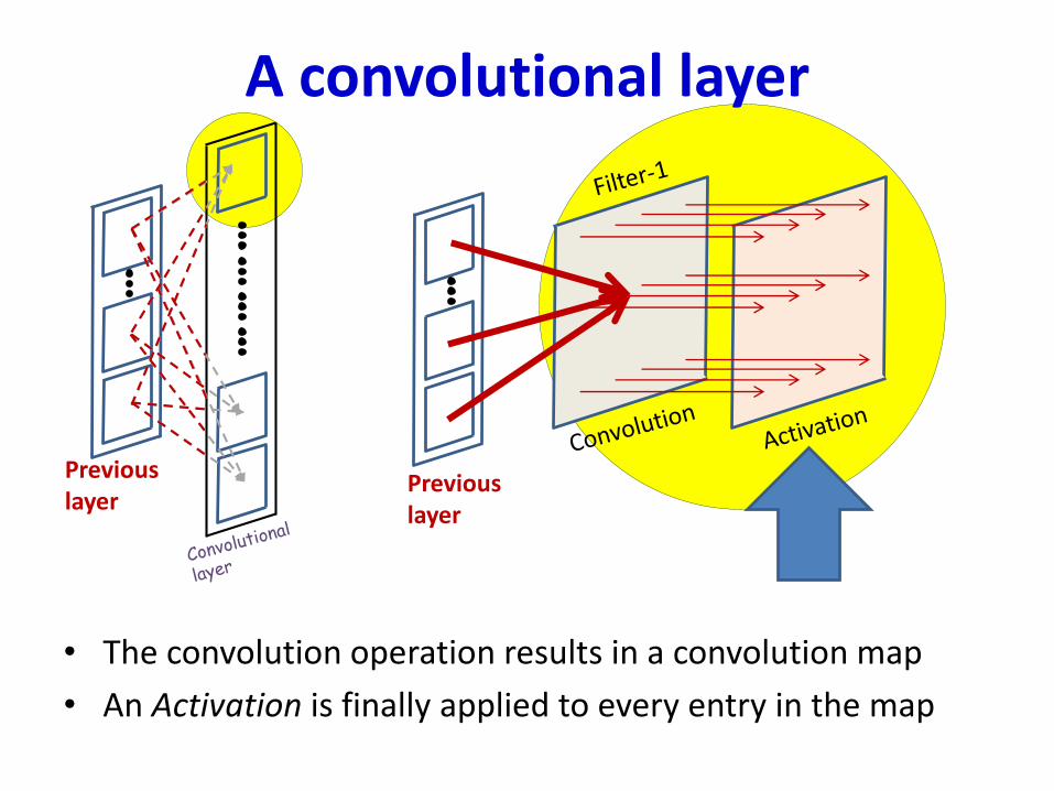
A convolutional layer
• The convolution operation results in a convolution map
• An Activation is finally applied to every entry in the map
Previouslayer
Previouslayer
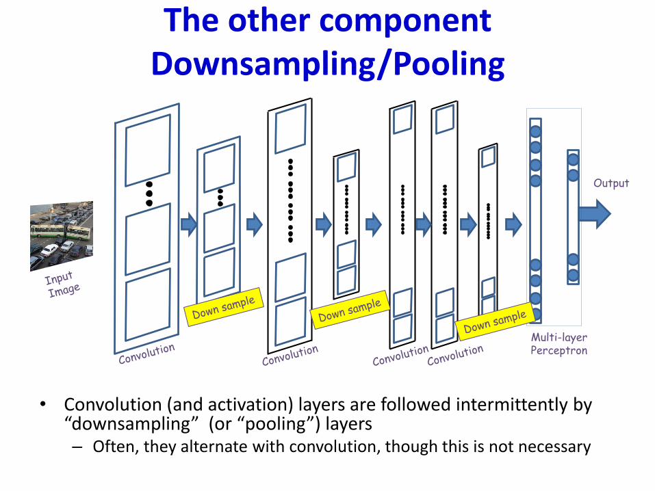
The other component Downsampling/Pooling
• Convolution (and activation) layers are followed intermittently by “downsampling” (or “pooling”) layers– Often, they alternate with convolution, though this is not necessary
Multi-layerPerceptron
Output
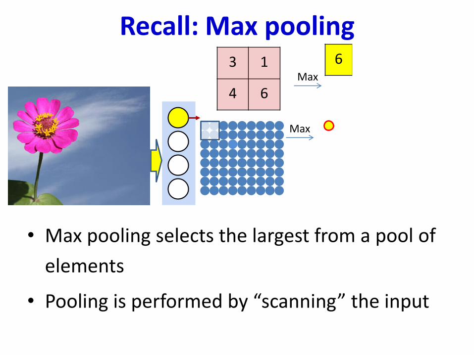
Recall: Max pooling
• Max pooling selects the largest from a pool of
elements
• Pooling is performed by “scanning” the input
Max
3 1
4 6Max
6
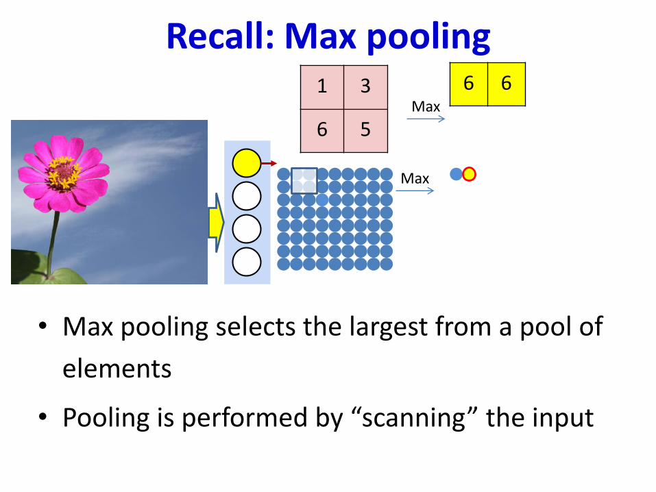
Recall: Max pooling
Max
1 3
6 5Max
6 6
• Max pooling selects the largest from a pool of
elements
• Pooling is performed by “scanning” the input
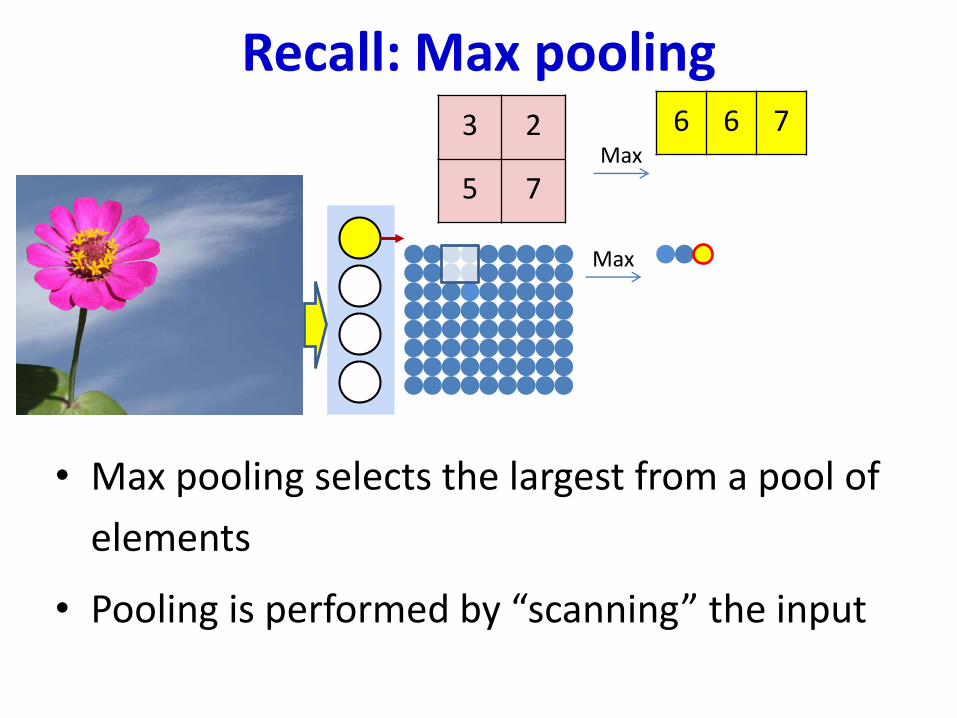
Recall: Max pooling
Max
3 2
5 7Max
6 6 7
• Max pooling selects the largest from a pool of
elements
• Pooling is performed by “scanning” the input
Recall: Max pooling
Max
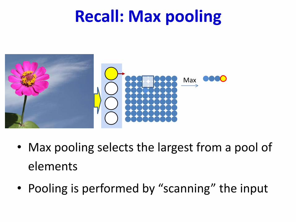
• Max pooling selects the largest from a pool of
elements
• Pooling is performed by “scanning” the input

Recall: Max pooling
Max
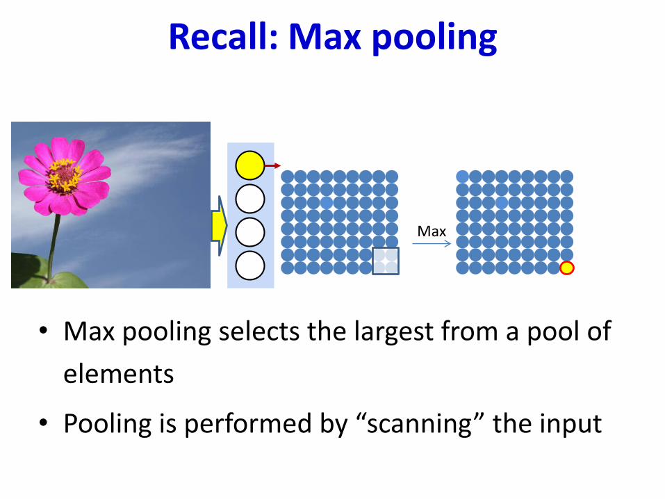
• Max pooling selects the largest from a pool of
elements
• Pooling is performed by “scanning” the input
Recall: Max pooling
Max
• Max pooling selects the largest from a pool of
elements
• Pooling is performed by “scanning” the input
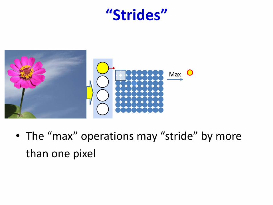
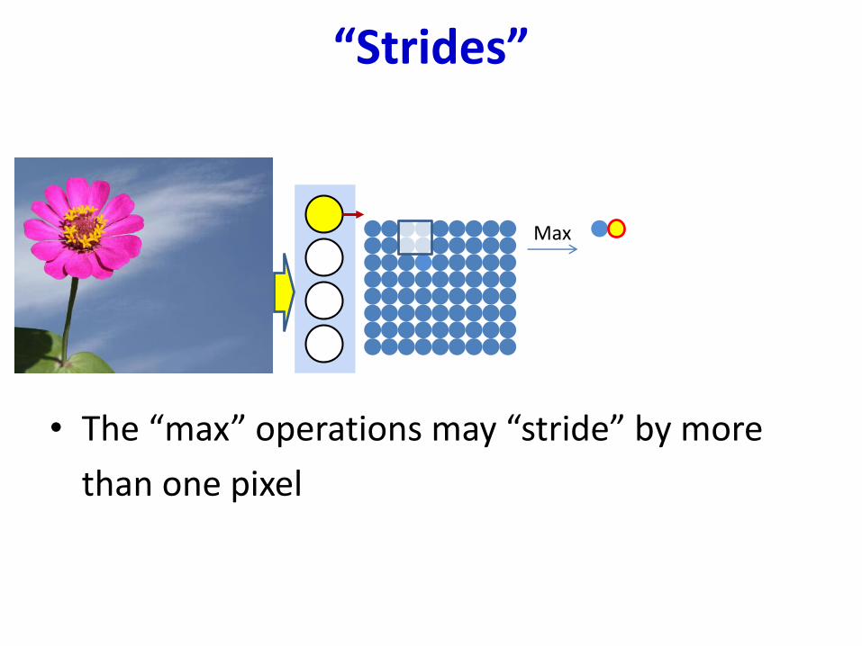
“Strides”
• The “max” operations may “stride” by more
than one pixel
Max
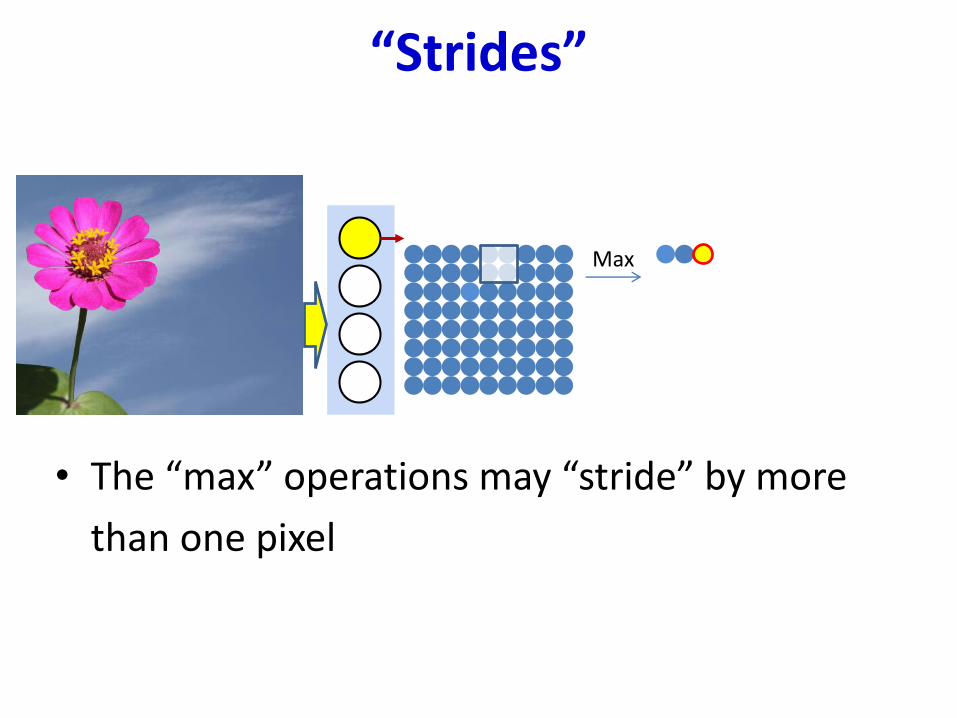
“Strides”
• The “max” operations may “stride” by more
than one pixel
Max
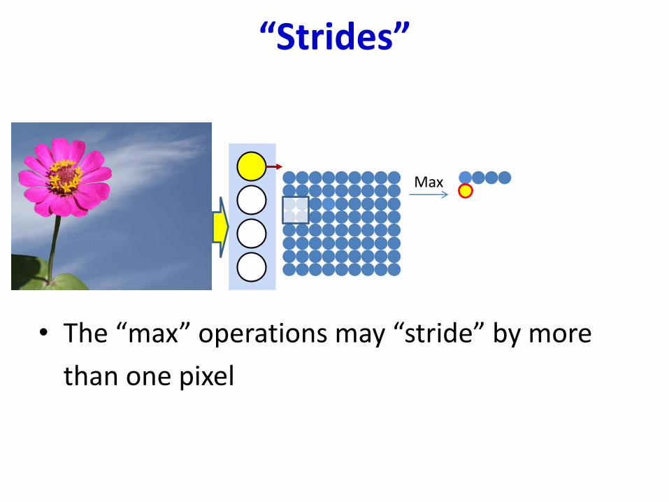
“Strides”
• The “max” operations may “stride” by more
than one pixel
Max
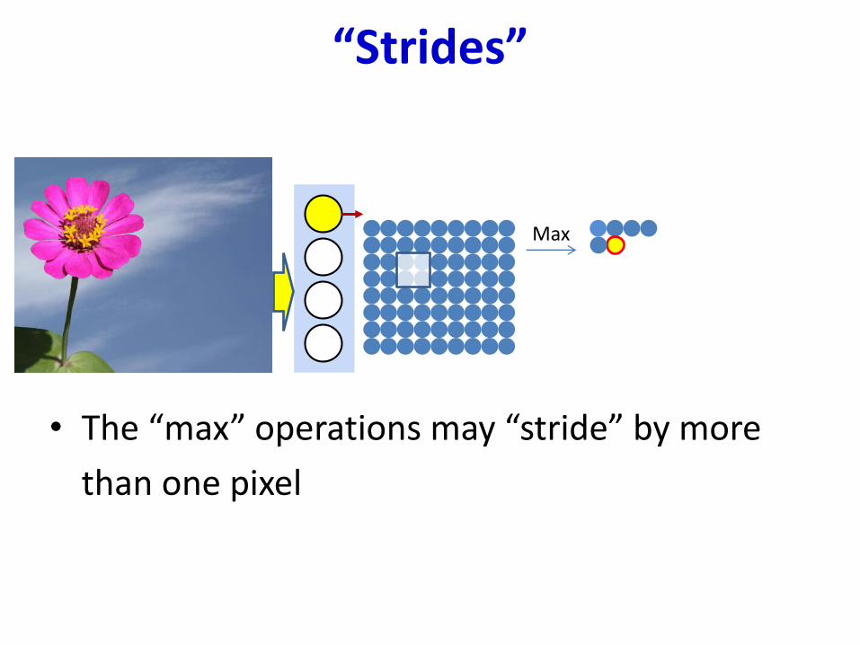
“Strides”
• The “max” operations may “stride” by more
than one pixel
Max
“Strides”
• The “max” operations may “stride” by more
than one pixel
Max
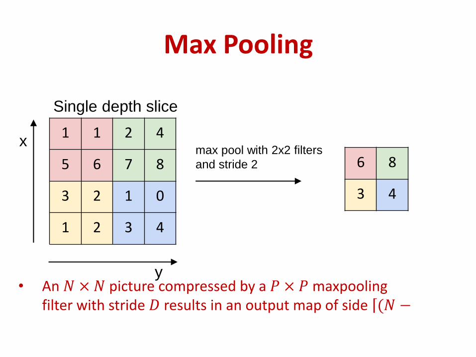
1 1 2 4
5 6 7 8
3 2 1 0
1 2 3 4
Single depth slice
x
y
max pool with 2x2 filters
and stride 2 6 8
3 4
Max Pooling
• An 𝑁 × 𝑁 picture compressed by a 𝑃 × 𝑃 maxpoolingfilter with stride 𝐷 results in an output map of side ڿ(𝑁 −
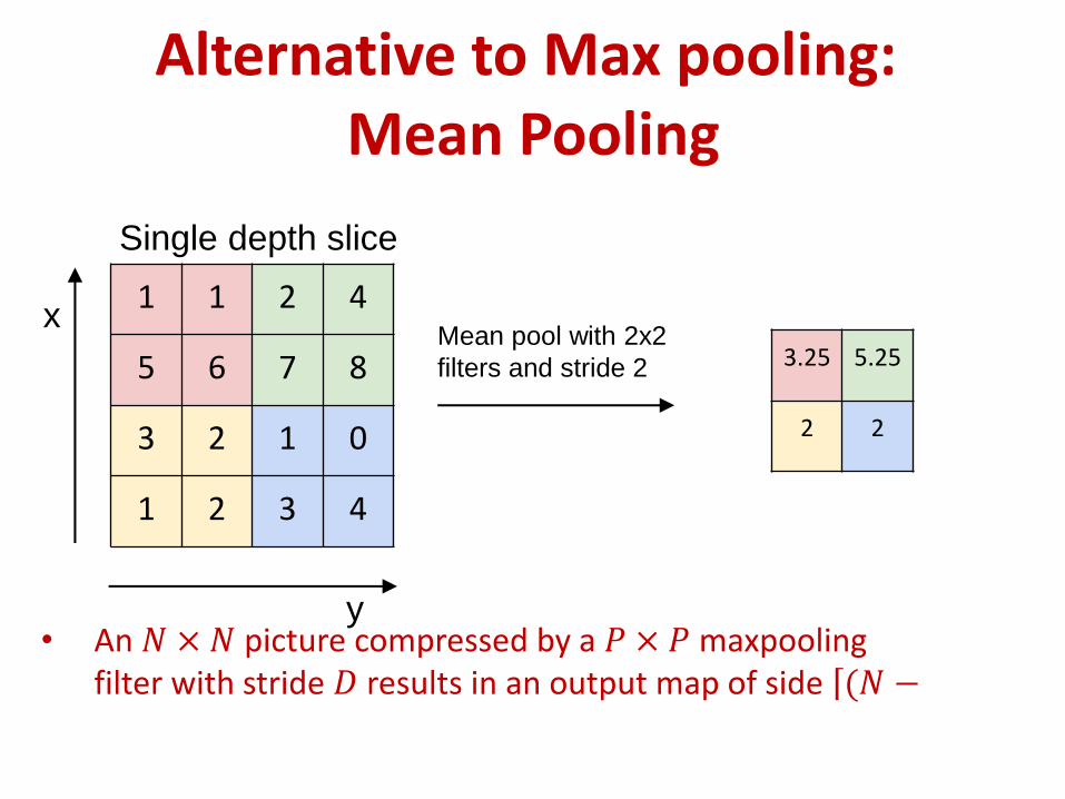
1 1 2 4
5 6 7 8
3 2 1 0
1 2 3 4
Single depth slice
x
y
Mean pool with 2x2
filters and stride 2 3.25 5.25
2 2
Alternative to Max pooling: Mean Pooling
• An 𝑁 × 𝑁 picture compressed by a 𝑃 × 𝑃 maxpoolingfilter with stride 𝐷 results in an output map of side ڿ(𝑁 −
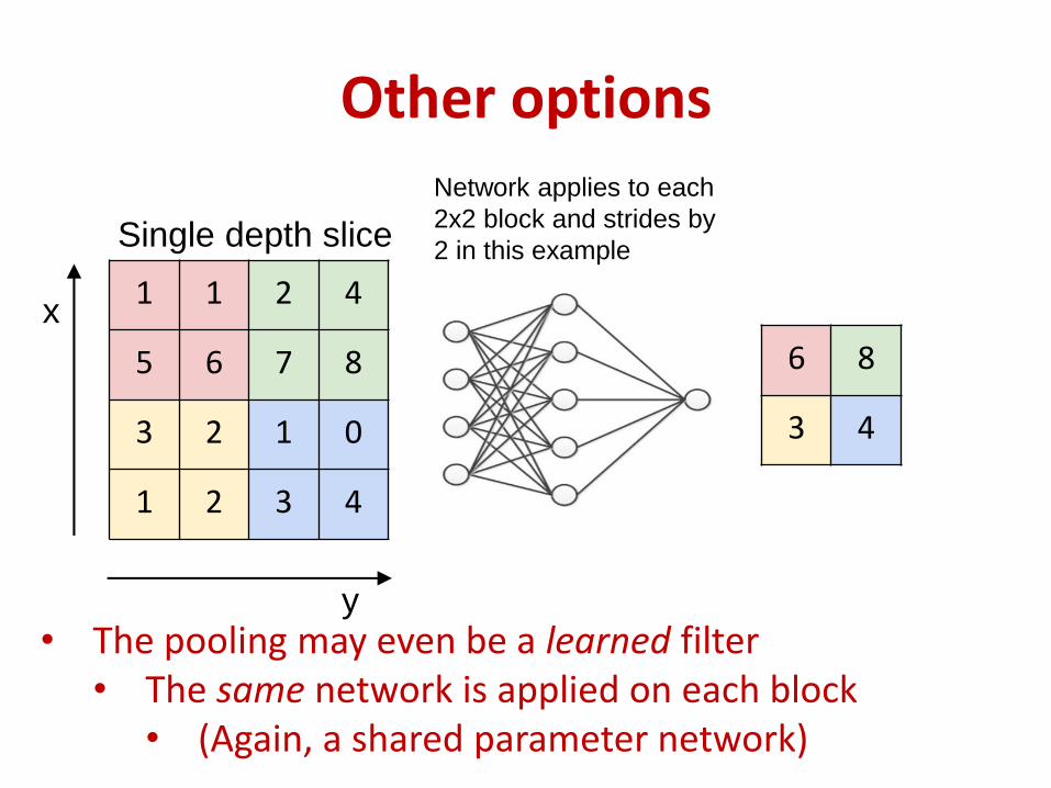
1 1 2 4
5 6 7 8
3 2 1 0
1 2 3 4
Single depth slice
x
y
Network applies to each
2x2 block and strides by
2 in this example
6 8
3 4
Other options
• The pooling may even be a learned filter• The same network is applied on each block
• (Again, a shared parameter network)
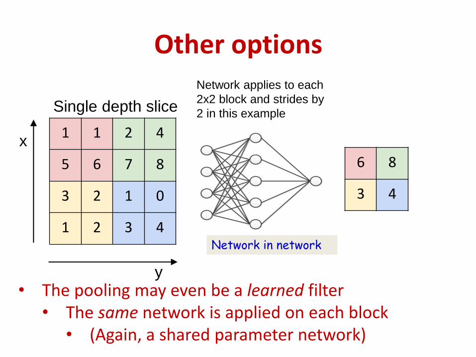
1 1 2 4
5 6 7 8
3 2 1 0
1 2 3 4
Single depth slice
x
y
Network applies to each
2x2 block and strides by
2 in this example
6 8
3 4
Other options
• The pooling may even be a learned filter• The same network is applied on each block
• (Again, a shared parameter network)
Network in network
Setting everything together
• Typical image classification task
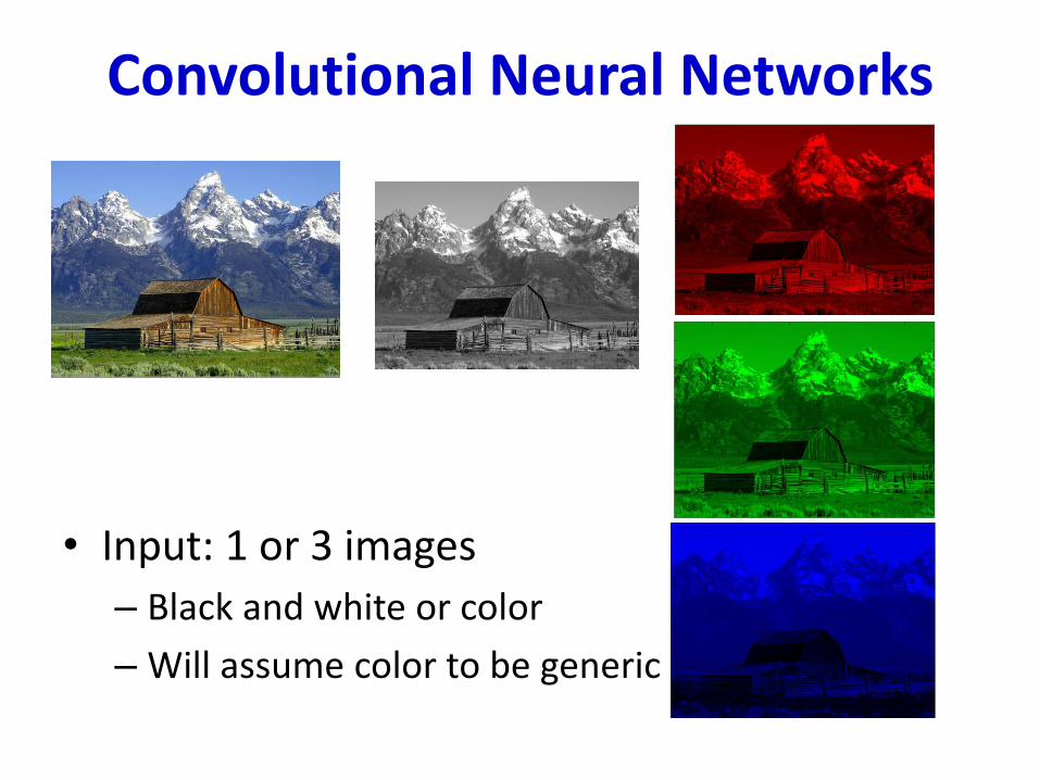
Convolutional Neural Networks
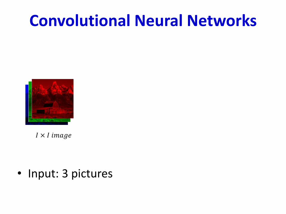
• Input: 1 or 3 images
– Black and white or color
– Will assume color to be generic
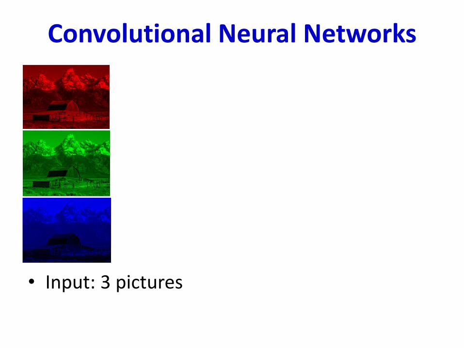
• Input: 3 pictures
Convolutional Neural Networks
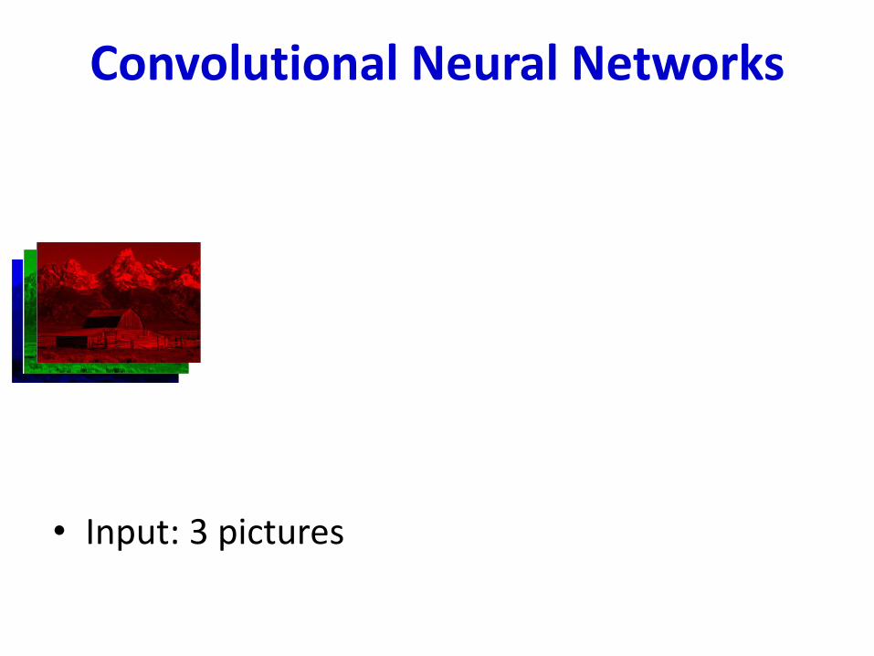
• Input: 3 pictures
Convolutional Neural Networks
Preprocessing
• Typically works with square images
– Filters are also typically square
• Large networks are a problem
– Too much detail
– Will need big networks
• Typically scaled to small sizes, e.g. 32x32 or 128x128
• Input: 3 pictures
Convolutional Neural Networks
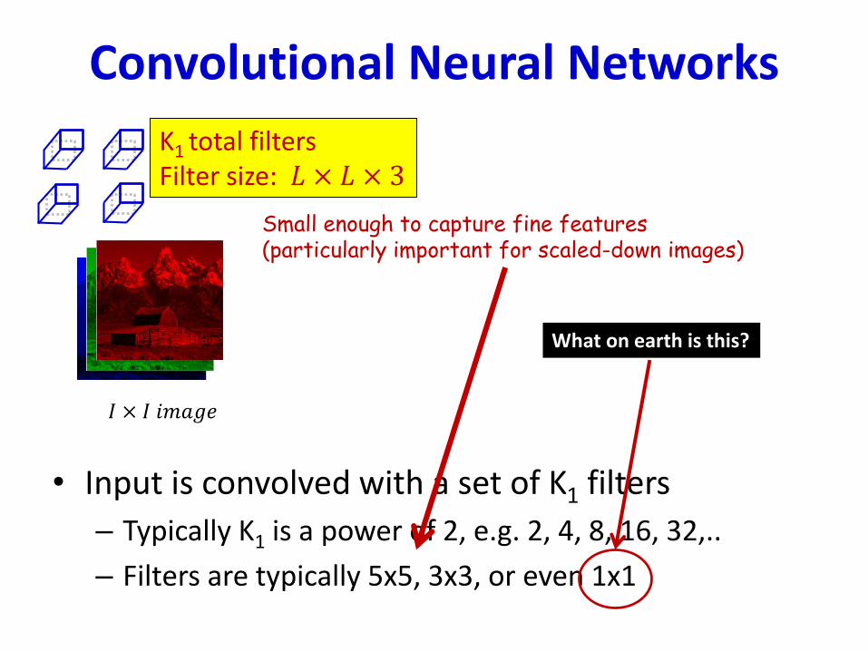
𝐼 × 𝐼 𝑖𝑚𝑎𝑔𝑒
• Input is convolved with a set of K1 filters
– Typically K1 is a power of 2, e.g. 2, 4, 8, 16, 32,..
– Filters are typically 5x5, 3x3, or even 1x1
Convolutional Neural Networks
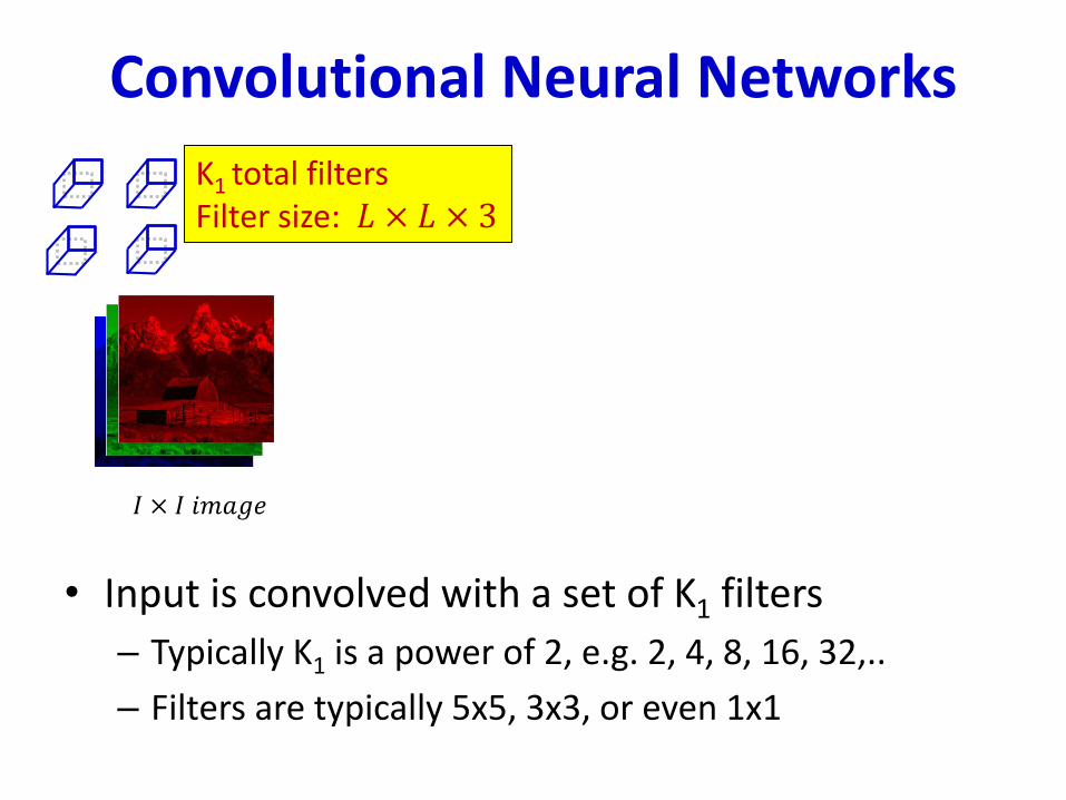
𝐼 × 𝐼 𝑖𝑚𝑎𝑔𝑒
K1 total filtersFilter size: 𝐿 × 𝐿 × 3
• Input is convolved with a set of K1 filters
– Typically K1 is a power of 2, e.g. 2, 4, 8, 16, 32,..
– Filters are typically 5x5, 3x3, or even 1x1
Convolutional Neural Networks
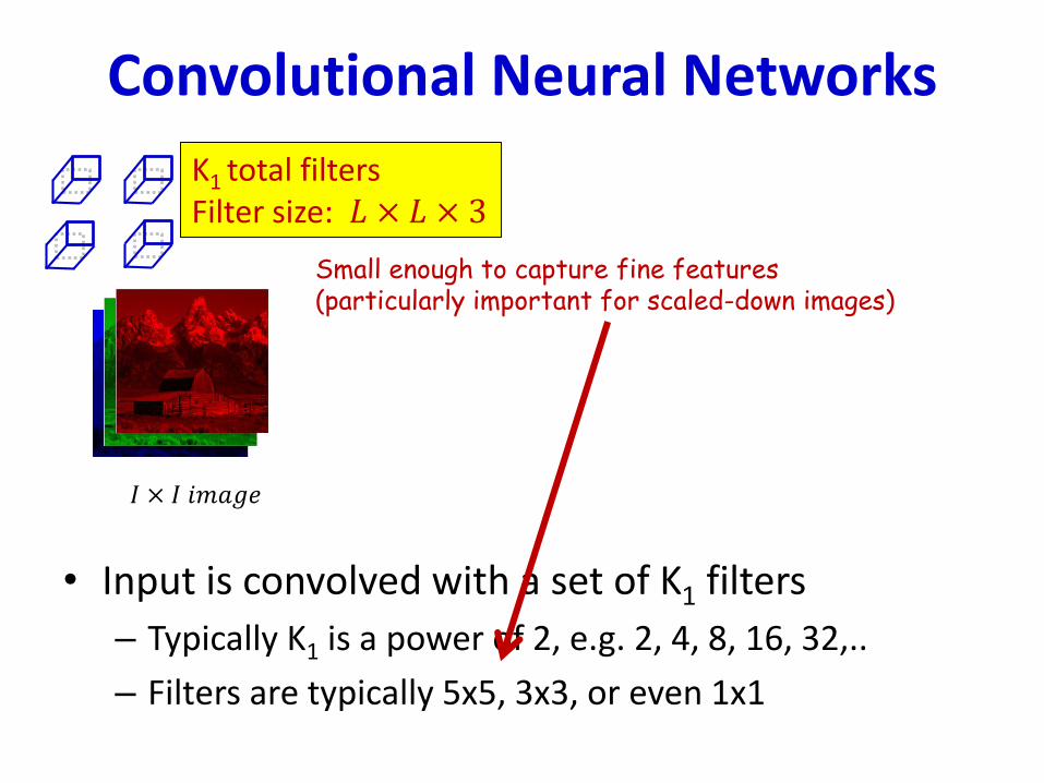
𝐼 × 𝐼 𝑖𝑚𝑎𝑔𝑒
Small enough to capture fine features(particularly important for scaled-down images)
K1 total filtersFilter size: 𝐿 × 𝐿 × 3
• Input is convolved with a set of K1 filters
– Typically K1 is a power of 2, e.g. 2, 4, 8, 16, 32,..
– Filters are typically 5x5, 3x3, or even 1x1
Convolutional Neural Networks
𝐼 × 𝐼 𝑖𝑚𝑎𝑔𝑒
What on earth is this?
Small enough to capture fine features(particularly important for scaled-down images)
K1 total filtersFilter size: 𝐿 × 𝐿 × 3
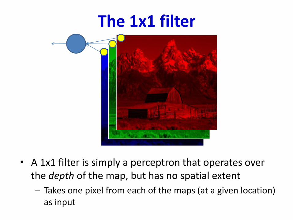
• A 1x1 filter is simply a perceptron that operates over the depth of the map, but has no spatial extent
– Takes one pixel from each of the maps (at a given location) as input
The 1x1 filter
• Input is convolved with a set of K1 filters
– Typically K1 is a power of 2, e.g. 2, 4, 8, 16, 32,..
– Better notation: Filters are typically 5x5(x3), 3x3(x3), or even 1x1(x3)
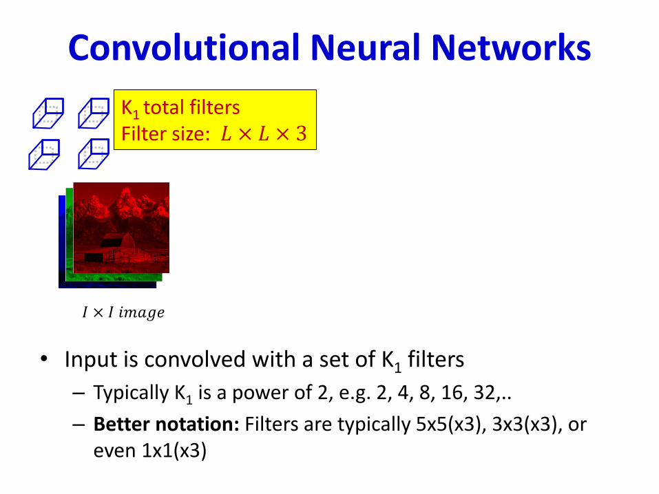
Convolutional Neural Networks
𝐼 × 𝐼 𝑖𝑚𝑎𝑔𝑒
K1 total filtersFilter size: 𝐿 × 𝐿 × 3
• Input is convolved with a set of K1 filters
– Typically K1 is a power of 2, e.g. 2, 4, 8, 16, 32,..
– Better notation: Filters are typically 5x5(x3), 3x3(x3), or even 1x1(x3)
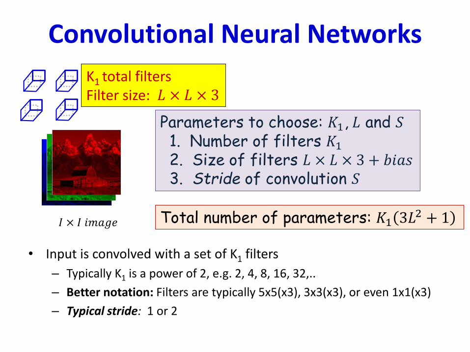
– Typical stride: 1 or 2
Convolutional Neural Networks
𝐼 × 𝐼 𝑖𝑚𝑎𝑔𝑒 Total number of parameters: 𝐾1 3𝐿2 + 1
Parameters to choose: 𝐾1, 𝐿 and 𝑆1. Number of filters 𝐾12. Size of filters 𝐿 × 𝐿 × 3 + 𝑏𝑖𝑎𝑠3. Stride of convolution 𝑆
K1 total filtersFilter size: 𝐿 × 𝐿 × 3
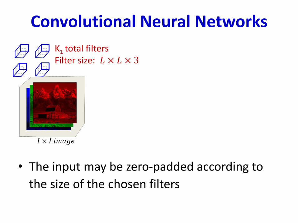
• The input may be zero-padded according to
the size of the chosen filters
Convolutional Neural Networks
𝐼 × 𝐼 𝑖𝑚𝑎𝑔𝑒
K1 total filtersFilter size: 𝐿 × 𝐿 × 3
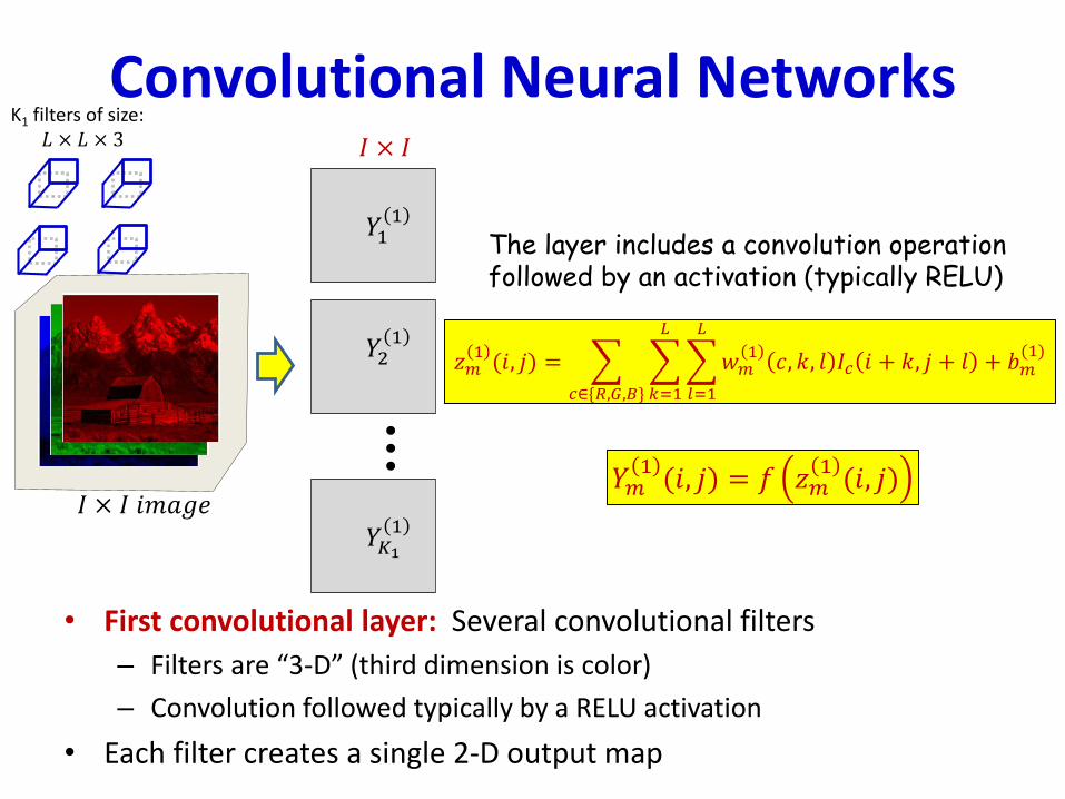
• First convolutional layer: Several convolutional filters
– Filters are “3-D” (third dimension is color)
– Convolution followed typically by a RELU activation
• Each filter creates a single 2-D output map
𝑌𝑚1(𝑖, 𝑗) = 𝑓 𝑧𝑚
1(𝑖, 𝑗)
𝑌11
𝑌21
𝑌𝐾11
𝐼 × 𝐼
Convolutional Neural Networks
𝐼 × 𝐼 𝑖𝑚𝑎𝑔𝑒
K1 filters of size: 𝐿 × 𝐿 × 3
𝑧𝑚1(𝑖, 𝑗) =
𝑐∈{𝑅,𝐺,𝐵}
𝑘=1
𝐿
𝑙=1
𝐿
𝑤𝑚1
𝑐, 𝑘, 𝑙 𝐼𝑐 𝑖 + 𝑘, 𝑗 + 𝑙 + 𝑏𝑚(1)
The layer includes a convolution operationfollowed by an activation (typically RELU)

Learnable parameters in the first convolutional layer
• The first convolutional layer comprises 𝐾1 filters, each of size 𝐿 × 𝐿 × 3
– Spatial span: 𝐿 × 𝐿
– Depth : 3 (3 colors)
• This represents a total of 𝐾1 3𝐿2 + 1 parameters
– “+ 1” because each filter also has a bias
• All of these parameters must be learned
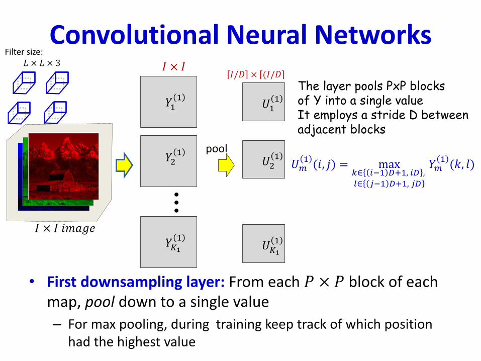
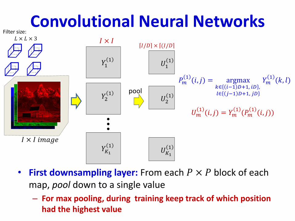
• First downsampling layer: From each 𝑃 × 𝑃 block of each map, pool down to a single value
– For max pooling, during training keep track of which position had the highest value
𝑈11
𝑈21
𝑈𝐾11
𝐼/𝐷 × (𝐼/𝐷
Convolutional Neural Networks
𝑌11
𝑌21
𝑌𝐾11
𝐼 × 𝐼
𝐼 × 𝐼 𝑖𝑚𝑎𝑔𝑒
Filter size: 𝐿 × 𝐿 × 3
pool
The layer pools PxP blocksof Y into a single valueIt employs a stride D betweenadjacent blocks
𝑈𝑚1(𝑖, 𝑗) = max
𝑘∈ 𝑖−1 𝐷+1, 𝑖𝐷 ,𝑙∈ 𝑗−1 𝐷+1, 𝑗𝐷
𝑌𝑚1(𝑘, 𝑙)
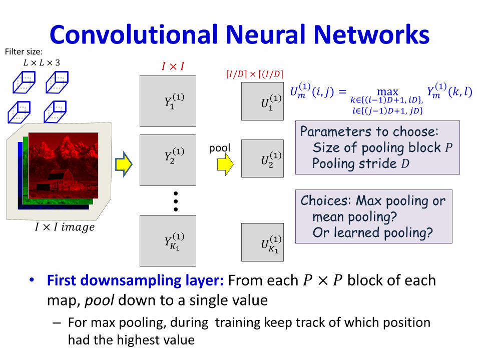
• First downsampling layer: From each 𝑃 × 𝑃 block of each map, pool down to a single value
– For max pooling, during training keep track of which position had the highest value
𝑈11
𝑈21
𝐼/𝐷 × (𝐼/𝐷
Convolutional Neural Networks
𝑌11
𝑌21
𝐼 × 𝐼
𝐼 × 𝐼 𝑖𝑚𝑎𝑔𝑒
Filter size: 𝐿 × 𝐿 × 3
Parameters to choose:Size of pooling block 𝑃Pooling stride 𝐷
pool
Choices: Max pooling ormean pooling?Or learned pooling?
𝑈𝐾11𝑌𝐾1
1
𝑈𝑚1(𝑖, 𝑗) = max
𝑘∈ 𝑖−1 𝐷+1, 𝑖𝐷 ,𝑙∈ 𝑗−1 𝐷+1, 𝑗𝐷
𝑌𝑚1(𝑘, 𝑙)
• First downsampling layer: From each 𝑃 × 𝑃 block of each map, pool down to a single value
– For max pooling, during training keep track of which position had the highest value
𝑈11
𝑈21
𝐼/𝐷 × (𝐼/𝐷
Convolutional Neural Networks
𝑌11
𝑌21
𝐼 × 𝐼
𝐼 × 𝐼 𝑖𝑚𝑎𝑔𝑒
Filter size: 𝐿 × 𝐿 × 3
pool
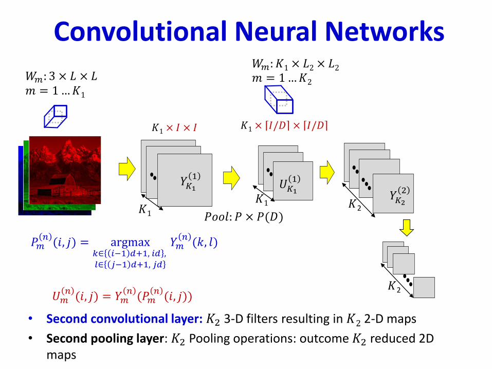
𝑈𝑚1(𝑖, 𝑗) = 𝑌𝑚
1(𝑃𝑚
1(𝑖, 𝑗))
𝑃𝑚1(𝑖, 𝑗) = argmax
𝑘∈ 𝑖−1 𝐷+1, 𝑖𝐷 ,𝑙∈ 𝑗−1 𝐷+1, 𝑗𝐷
𝑌𝑚1(𝑘, 𝑙)
𝑈𝐾11𝑌𝐾1
1
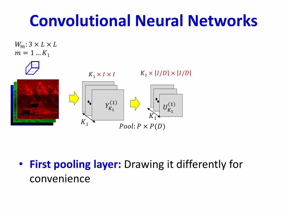
• First pooling layer: Drawing it differently for convenience
𝑊𝑚: 3 × 𝐿 × 𝐿𝑚 = 1…𝐾1
𝑌11𝑌2
1
𝐾1 𝑃𝑜𝑜𝑙: 𝑃 × 𝑃(𝐷)
𝐾1 × 𝐼 × 𝐼 𝐾1 × 𝐼/𝐷 × 𝐼/𝐷
Convolutional Neural Networks
𝐾1
𝑈𝐾11𝑌𝐾1
1
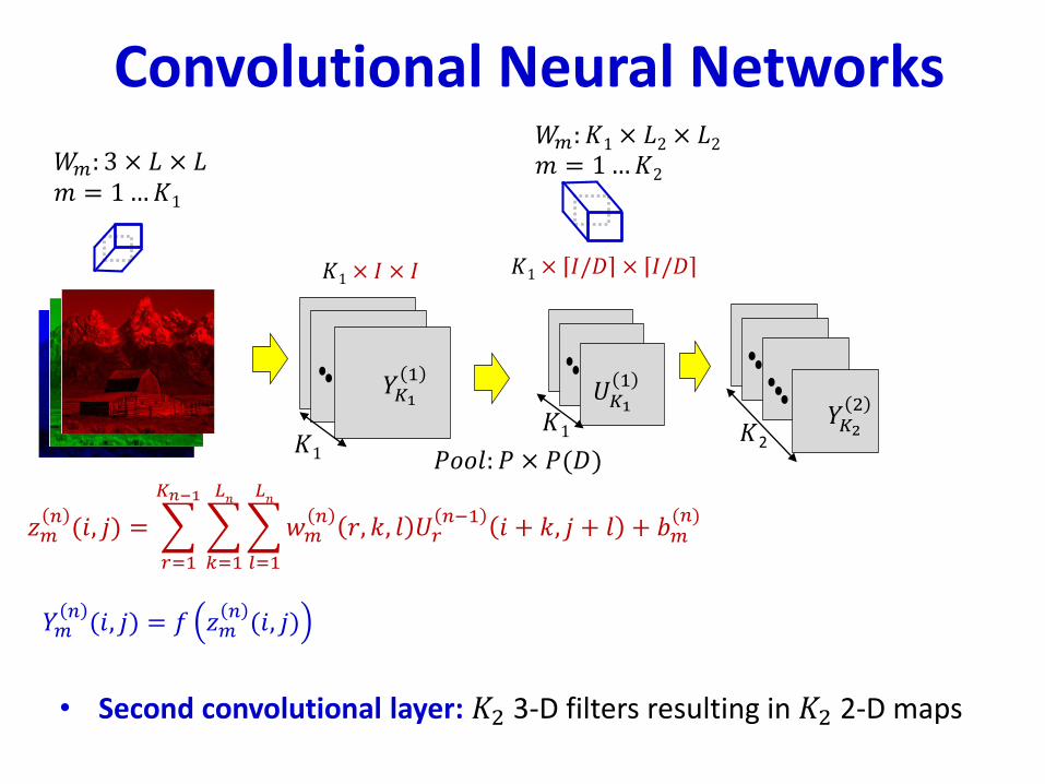
• Second convolutional layer: 𝐾2 3-D filters resulting in 𝐾2 2-D maps
𝑊𝑚: 𝐾1 × 𝐿2 × 𝐿2𝑚 = 1…𝐾2
𝑌𝐾22
𝐾2
𝑌𝑚𝑛(𝑖, 𝑗) = 𝑓 𝑧𝑚
𝑛(𝑖, 𝑗)
𝑧𝑚𝑛(𝑖, 𝑗) =
𝑟=1
𝐾𝑛−1
𝑘=1
𝐿𝑛
𝑙=1
𝐿𝑛
𝑤𝑚𝑛
𝑟, 𝑘, 𝑙 𝑈𝑟𝑛−1
𝑖 + 𝑘, 𝑗 + 𝑙 + 𝑏𝑚(𝑛)
Convolutional Neural Networks
𝑊𝑚: 3 × 𝐿 × 𝐿𝑚 = 1…𝐾1
𝑌11𝑌2
1
𝐾1 𝑃𝑜𝑜𝑙: 𝑃 × 𝑃(𝐷)
𝐾1 × 𝐼 × 𝐼 𝐾1 × 𝐼/𝐷 × 𝐼/𝐷
𝐾1
𝑈𝐾11𝑌𝐾1
1
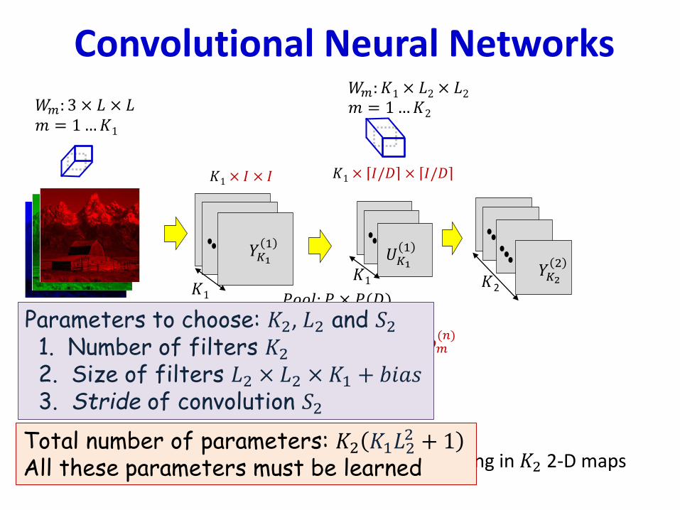
Total number of parameters: 𝐾2 𝐾1𝐿22 + 1
All these parameters must be learned
Parameters to choose: 𝐾2, 𝐿2 and 𝑆21. Number of filters 𝐾22. Size of filters 𝐿2 × 𝐿2 × 𝐾1 + 𝑏𝑖𝑎𝑠3. Stride of convolution 𝑆2
𝑊𝑚: 𝐾1 × 𝐿2 × 𝐿2𝑚 = 1…𝐾2
𝑌𝐾22
𝐾2
Convolutional Neural Networks
𝑊𝑚: 3 × 𝐿 × 𝐿𝑚 = 1…𝐾1
𝑌11𝑌2
1
𝐾1 𝑃𝑜𝑜𝑙: 𝑃 × 𝑃(𝐷)
𝐾1 × 𝐼 × 𝐼 𝐾1 × 𝐼/𝐷 × 𝐼/𝐷
𝐾1
𝐾2
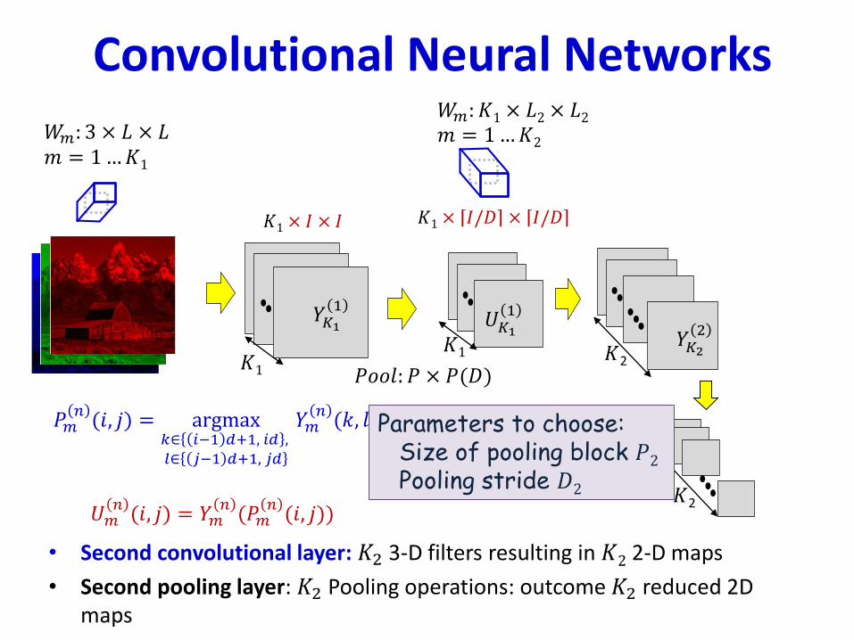
• Second convolutional layer: 𝐾2 3-D filters resulting in 𝐾2 2-D maps
• Second pooling layer: 𝐾2 Pooling operations: outcome 𝐾2 reduced 2D maps
𝑈𝑚𝑛(𝑖, 𝑗) = 𝑌𝑚
𝑛(𝑃𝑚
𝑛(𝑖, 𝑗))
𝑃𝑚𝑛(𝑖, 𝑗) = argmax
𝑘∈ 𝑖−1 𝑑+1, 𝑖𝑑 ,𝑙∈ 𝑗−1 𝑑+1, 𝑗𝑑
𝑌𝑚𝑛(𝑘, 𝑙)
𝑈𝐾11𝑌𝐾1
1
𝑊𝑚: 𝐾1 × 𝐿2 × 𝐿2𝑚 = 1…𝐾2
𝑌𝐾22
𝐾2
Convolutional Neural Networks
𝑊𝑚: 3 × 𝐿 × 𝐿𝑚 = 1…𝐾1
𝑌11𝑌2
1
𝐾1 𝑃𝑜𝑜𝑙: 𝑃 × 𝑃(𝐷)
𝐾1 × 𝐼 × 𝐼 𝐾1 × 𝐼/𝐷 × 𝐼/𝐷
𝐾1
𝐾2
• Second convolutional layer: 𝐾2 3-D filters resulting in 𝐾2 2-D maps
• Second pooling layer: 𝐾2 Pooling operations: outcome 𝐾2 reduced 2D maps
𝑈𝑚𝑛(𝑖, 𝑗) = 𝑌𝑚
𝑛(𝑃𝑚
𝑛(𝑖, 𝑗))
𝑃𝑚𝑛(𝑖, 𝑗) = argmax
𝑘∈ 𝑖−1 𝑑+1, 𝑖𝑑 ,𝑙∈ 𝑗−1 𝑑+1, 𝑗𝑑
𝑌𝑚𝑛(𝑘, 𝑙)
𝑈𝐾11𝑌𝐾1
1
Parameters to choose:Size of pooling block 𝑃2Pooling stride 𝐷2
𝑊𝑚: 𝐾1 × 𝐿2 × 𝐿2𝑚 = 1…𝐾2
𝑌𝐾22
𝐾2
Convolutional Neural Networks
𝑊𝑚: 3 × 𝐿 × 𝐿𝑚 = 1…𝐾1
𝑌11𝑌2
1
𝐾1 𝑃𝑜𝑜𝑙: 𝑃 × 𝑃(𝐷)
𝐾1 × 𝐼 × 𝐼 𝐾1 × 𝐼/𝐷 × 𝐼/𝐷
𝐾1
𝐾2
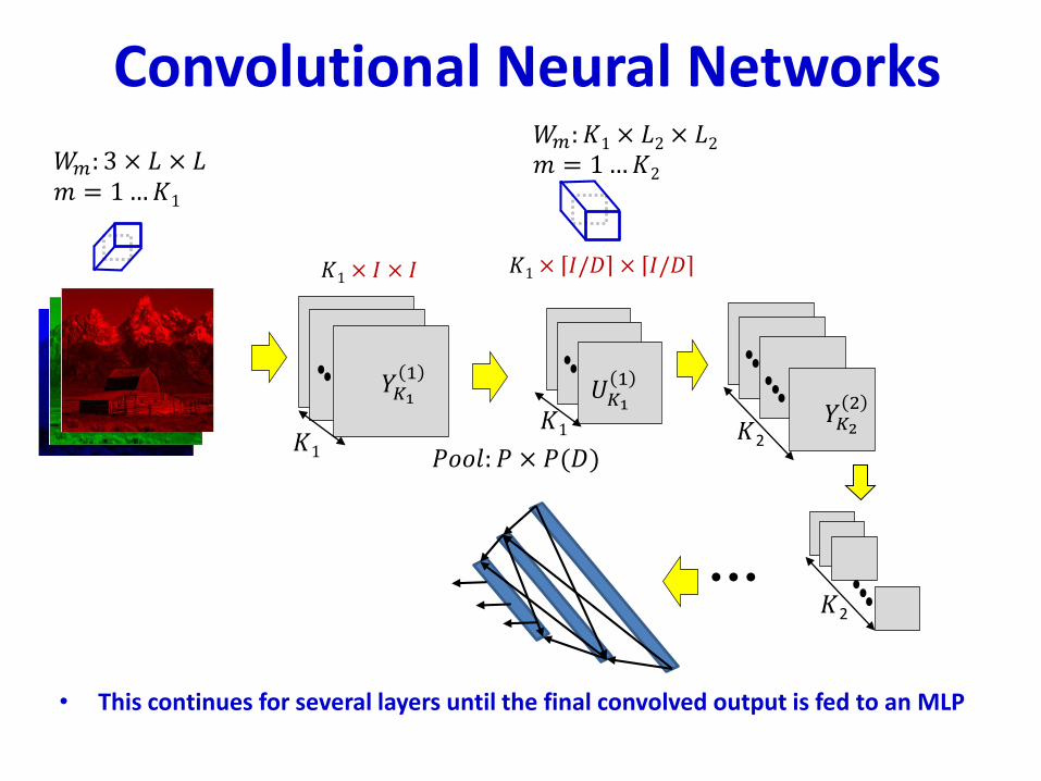
• This continues for several layers until the final convolved output is fed to an MLP
𝑈𝐾11𝑌𝐾1
1
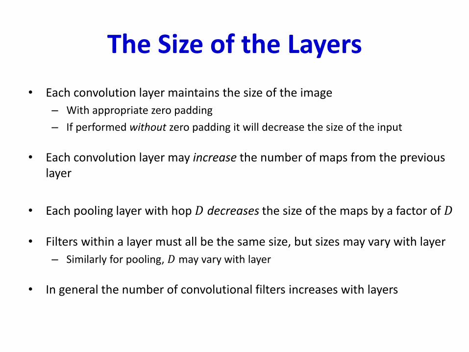
The Size of the Layers
• Each convolution layer maintains the size of the image
– With appropriate zero padding
– If performed without zero padding it will decrease the size of the input
• Each convolution layer may increase the number of maps from the previous layer
• Each pooling layer with hop 𝐷 decreases the size of the maps by a factor of 𝐷
• Filters within a layer must all be the same size, but sizes may vary with layer
– Similarly for pooling, 𝐷 may vary with layer
• In general the number of convolutional filters increases with layers
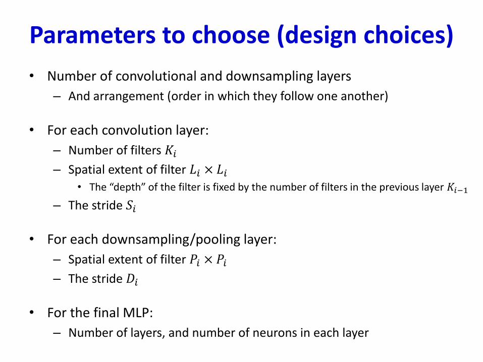
Parameters to choose (design choices)
• Number of convolutional and downsampling layers
– And arrangement (order in which they follow one another)
• For each convolution layer:
– Number of filters 𝐾𝑖– Spatial extent of filter 𝐿𝑖 × 𝐿𝑖
• The “depth” of the filter is fixed by the number of filters in the previous layer 𝐾𝑖−1
– The stride 𝑆𝑖
• For each downsampling/pooling layer:
– Spatial extent of filter 𝑃𝑖 × 𝑃𝑖– The stride 𝐷𝑖
• For the final MLP:
– Number of layers, and number of neurons in each layer
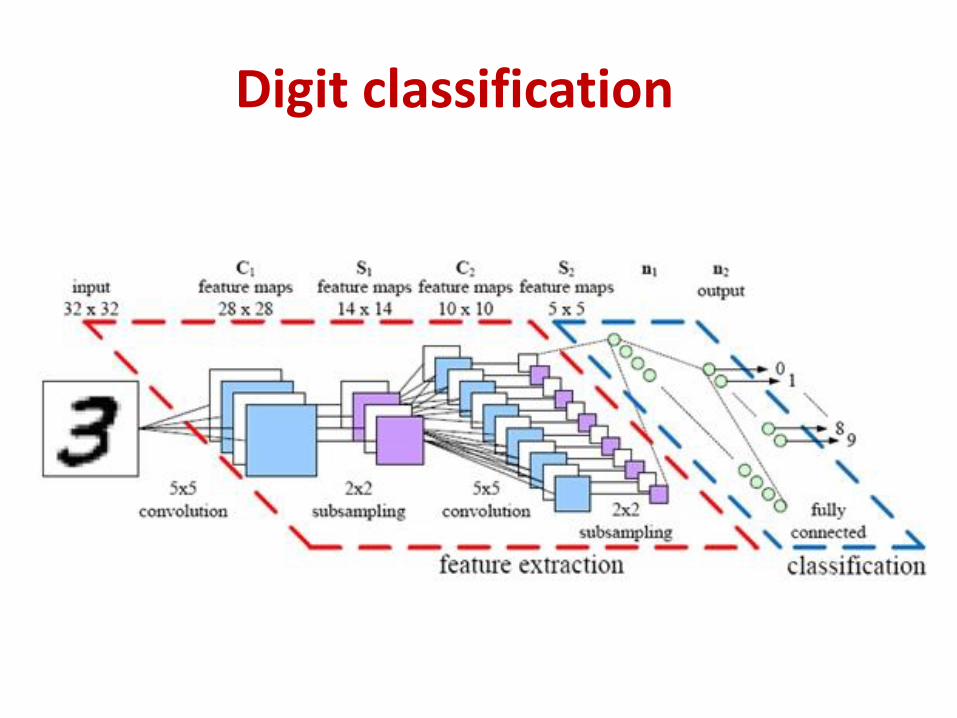
Digit classification
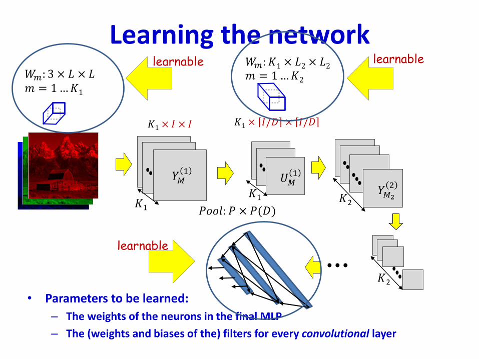
Learning the network
• Parameters to be learned:
– The weights of the neurons in the final MLP
– The (weights and biases of the) filters for every convolutional layer
𝑊𝑚: 𝐾1 × 𝐿2 × 𝐿2𝑚 = 1…𝐾2
𝑌𝑀2
2
𝐾2
𝑊𝑚: 3 × 𝐿 × 𝐿𝑚 = 1…𝐾1
𝑌11𝑌2
1
𝑌𝑀1
𝐾1
𝑈𝑀1
𝑃𝑜𝑜𝑙: 𝑃 × 𝑃(𝐷)
𝐾1 × 𝐼 × 𝐼 𝐾1 × 𝐼/𝐷 × 𝐼/𝐷
𝐾1
𝐾2
learnable learnable
learnable
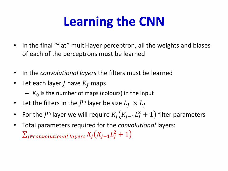
Learning the CNN
• In the final “flat” multi-layer perceptron, all the weights and biases of each of the perceptrons must be learned
• In the convolutional layers the filters must be learned
• Let each layer 𝐽 have 𝐾𝐽 maps
– 𝐾0 is the number of maps (colours) in the input
• Let the filters in the 𝐽th layer be size 𝐿𝐽 × 𝐿𝐽
• For the 𝐽th layer we will require 𝐾𝐽 𝐾𝐽−1𝐿𝐽2 + 1 filter parameters
• Total parameters required for the convolutional layers:
σ𝐽∈𝑐𝑜𝑛𝑣𝑜𝑙𝑢𝑡𝑖𝑜𝑛𝑎𝑙 𝑙𝑎𝑦𝑒𝑟𝑠𝐾𝐽 𝐾𝐽−1𝐿𝐽2 + 1
Training
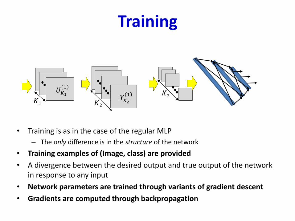
• Training is as in the case of the regular MLP
– The only difference is in the structure of the network
• Training examples of (Image, class) are provided
• A divergence between the desired output and true output of the network in response to any input
• Network parameters are trained through variants of gradient descent
• Gradients are computed through backpropagation
𝑈𝐾11
𝐾1𝑌𝐾2
1
𝐾2
𝐾2
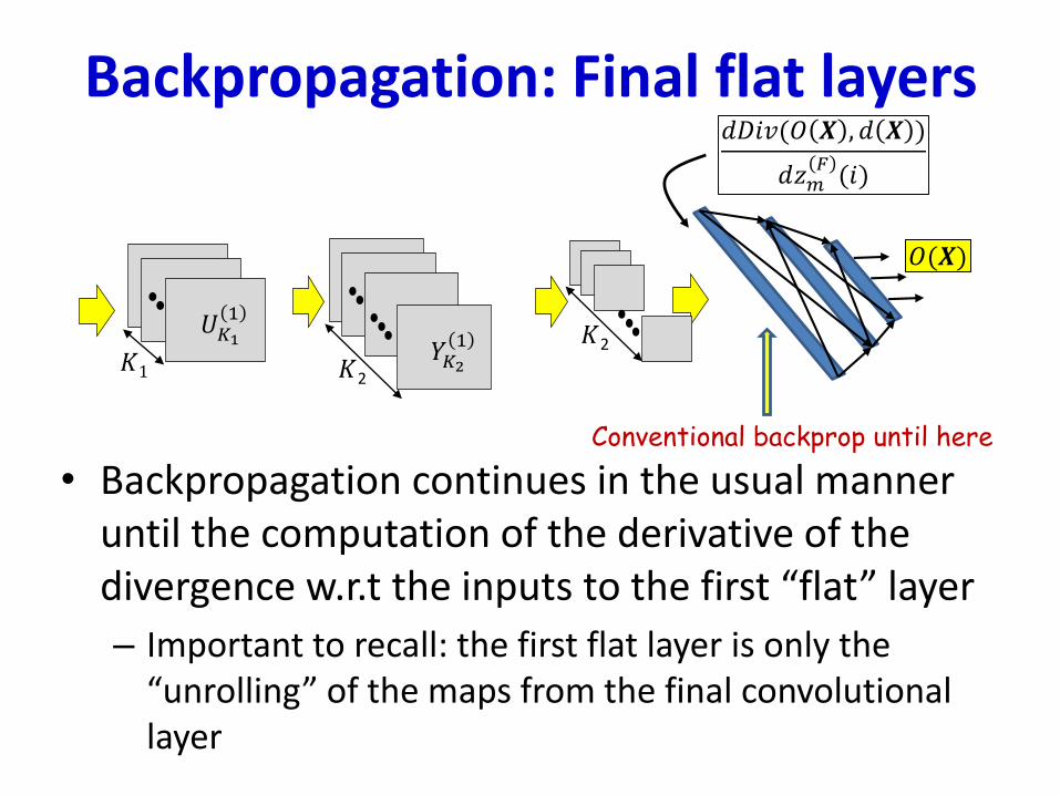
Backpropagation: Final flat layers
• Backpropagation continues in the usual manner until the computation of the derivative of the divergence w.r.t the inputs to the first “flat” layer
– Important to recall: the first flat layer is only the “unrolling” of the maps from the final convolutional layer
𝑑𝐷𝑖𝑣(𝑂 𝑿 , 𝑑 𝑿 )
𝑑𝑧𝑚𝐹(𝑖)
𝑂(𝑿)
𝑈𝐾11
𝐾1𝑌𝐾2
1
𝐾2
𝐾2
Conventional backprop until here
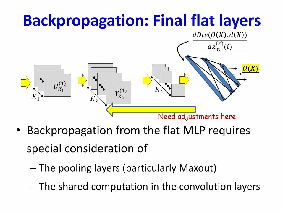
Backpropagation: Final flat layers
• Backpropagation from the flat MLP requires
special consideration of
– The pooling layers (particularly Maxout)
– The shared computation in the convolution layers
𝑑𝐷𝑖𝑣(𝑂 𝑿 , 𝑑 𝑿 )
𝑑𝑧𝑚𝐹(𝑖)
𝑂(𝑿)
𝑈𝐾11
𝐾1𝑌𝐾2
1
𝐾2
𝐾2
Need adjustments here
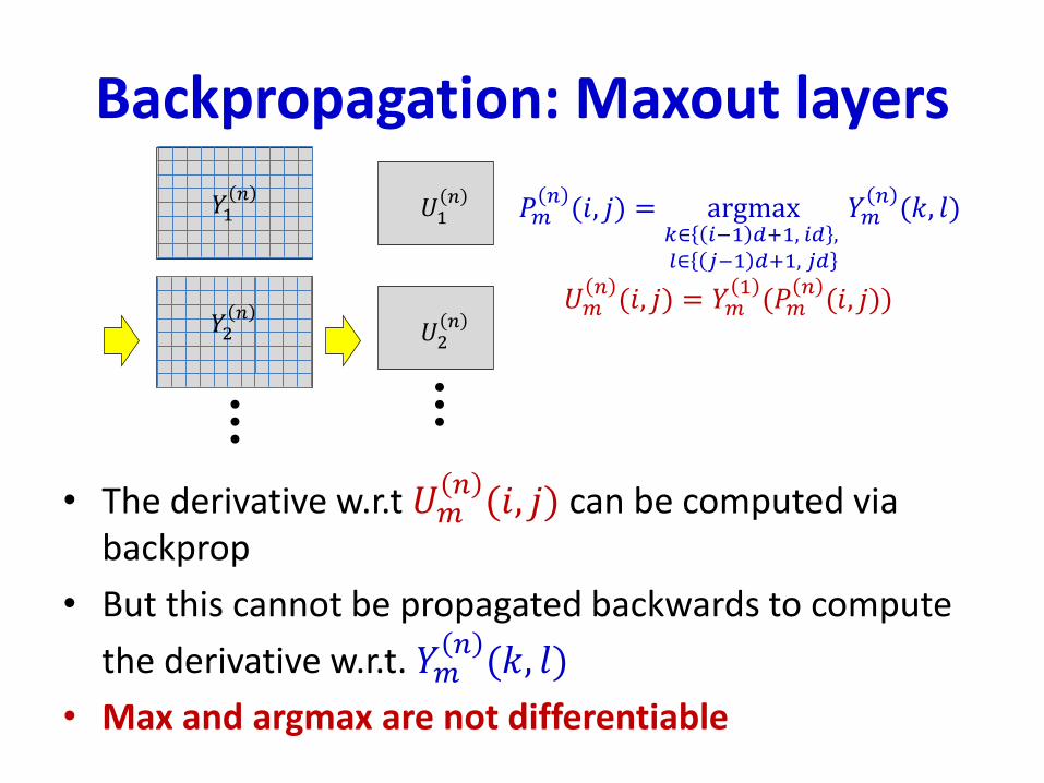
Backpropagation: Maxout layers
• The derivative w.r.t 𝑈𝑚𝑛(𝑖, 𝑗) can be computed via
backprop
• But this cannot be propagated backwards to compute
the derivative w.r.t. 𝑌𝑚𝑛(𝑘, 𝑙)
• Max and argmax are not differentiable
𝑈1𝑛
𝑈2𝑛
𝑈𝑚𝑛(𝑖, 𝑗) = 𝑌𝑚
1(𝑃𝑚
𝑛(𝑖, 𝑗))
𝑃𝑚𝑛(𝑖, 𝑗) = argmax
𝑘∈ 𝑖−1 𝑑+1, 𝑖𝑑 ,𝑙∈ 𝑗−1 𝑑+1, 𝑗𝑑
𝑌𝑚𝑛(𝑘, 𝑙)𝑌1
𝑛
𝑌2𝑛
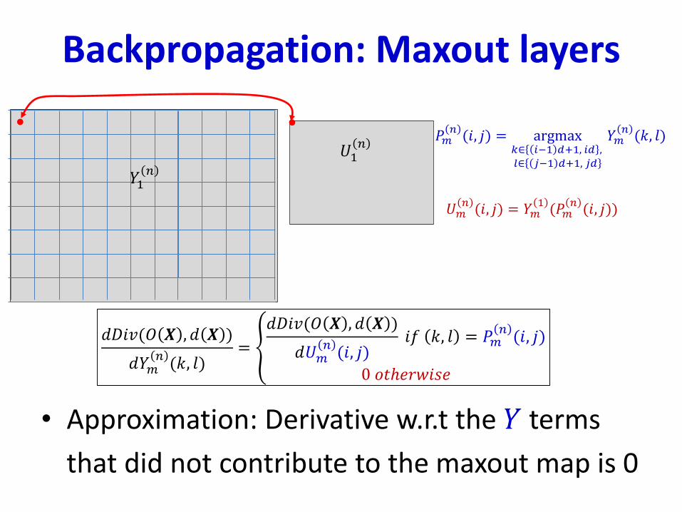
Backpropagation: Maxout layers
• Approximation: Derivative w.r.t the 𝑌 terms
that did not contribute to the maxout map is 0
𝑈1𝑛
𝑈𝑚𝑛(𝑖, 𝑗) = 𝑌𝑚
1(𝑃𝑚
𝑛(𝑖, 𝑗))
𝑃𝑚𝑛(𝑖, 𝑗) = argmax
𝑘∈ 𝑖−1 𝑑+1, 𝑖𝑑 ,𝑙∈ 𝑗−1 𝑑+1, 𝑗𝑑
𝑌𝑚𝑛(𝑘, 𝑙)
𝑌1𝑛
𝑑𝐷𝑖𝑣(𝑂 𝑿 , 𝑑 𝑿 )
𝑑𝑌𝑚𝑛(𝑘, 𝑙)
= ൞
𝑑𝐷𝑖𝑣(𝑂 𝑿 , 𝑑 𝑿 )
𝑑𝑈𝑚𝑛(𝑖, 𝑗)
𝑖𝑓 𝑘, 𝑙 = 𝑃𝑚𝑛(𝑖, 𝑗)
0 𝑜𝑡ℎ𝑒𝑟𝑤𝑖𝑠𝑒
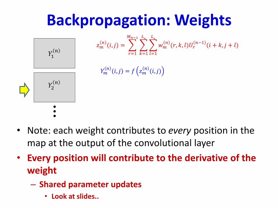
Backpropagation: Weights
• Note: each weight contributes to every position in the map at the output of the convolutional layer
• Every position will contribute to the derivative of the weight
– Shared parameter updates• Look at slides..
𝑌1𝑛
𝑌2𝑛
𝑌𝑚𝑛(𝑖, 𝑗) = 𝑓 𝑧𝑚
𝑛(𝑖, 𝑗)
𝑧𝑚𝑛(𝑖, 𝑗) =
𝑟=1
𝑀𝑛−1
𝑘=1
𝐿𝑛
𝑙=1
𝐿𝑛
𝑤𝑚𝑛(𝑟, 𝑘, 𝑙)𝑈𝑟
𝑛−1(𝑖 + 𝑘, 𝑗 + 𝑙)
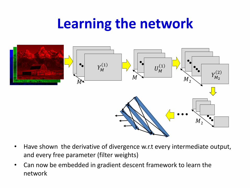
Learning the network
• Have shown the derivative of divergence w.r.t every intermediate output, and every free parameter (filter weights)
• Can now be embedded in gradient descent framework to learn the network
𝑌11𝑌2
1
𝑌𝑀1
𝑈𝑀1
𝑀𝑀 𝑌𝑀2
2
𝑀2
𝑀2
Training Issues
• Standard convergence issues– Solution: RMS prop or other momentum-style
algorithms
– Other tricks such as batch normalization
• The number of parameters can quickly become very large
• Insufficient training data to train well– Solution: Data augmentation
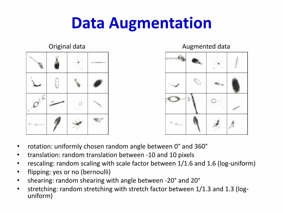
Data Augmentation
• rotation: uniformly chosen random angle between 0° and 360°• translation: random translation between -10 and 10 pixels• rescaling: random scaling with scale factor between 1/1.6 and 1.6 (log-uniform)• flipping: yes or no (bernoulli)• shearing: random shearing with angle between -20° and 20°• stretching: random stretching with stretch factor between 1/1.3 and 1.3 (log-
uniform)
Original data Augmented data
Other tricks
• Very deep networks
– 100 or more layers in MLP
– Formalism called “Resnet”
Convolutional neural nets
• One of the most frequently used nnetformalism today
• Used everywhere
– Not just for image classification
– Used in speech and audio processing
• Convnets on spectrograms

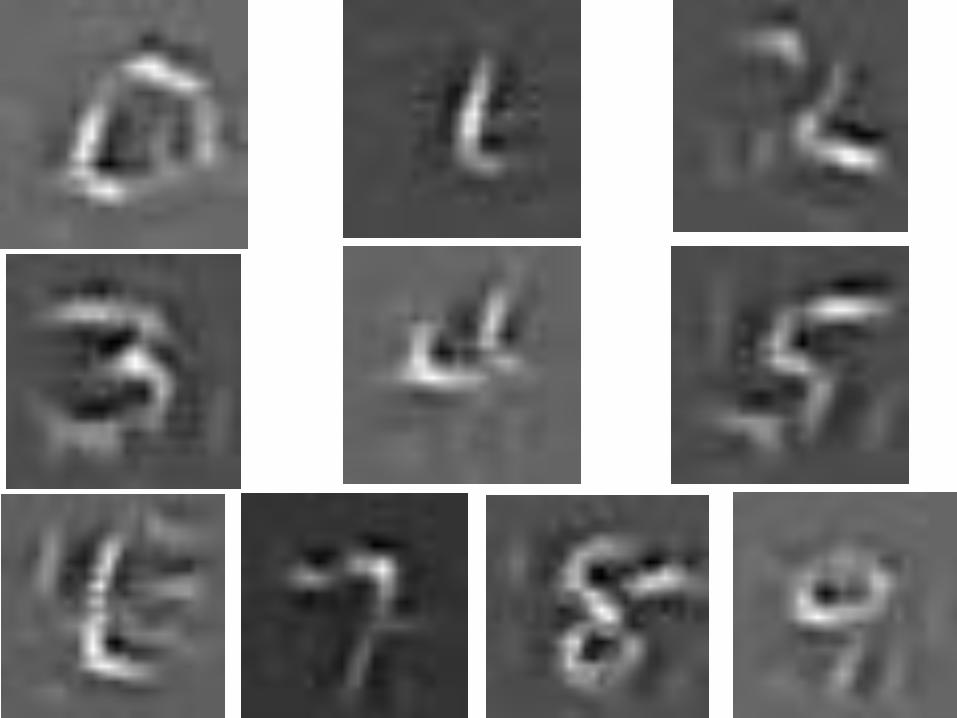
Digit classification
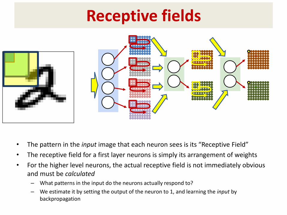
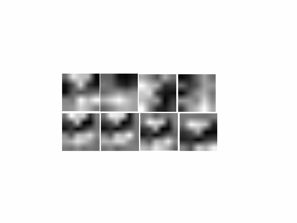
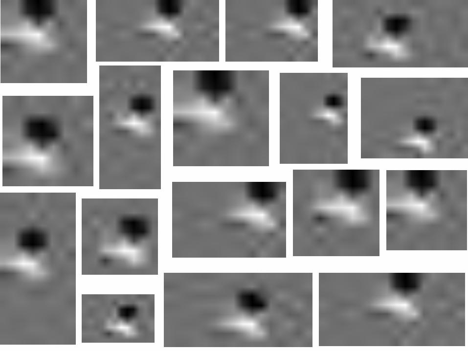
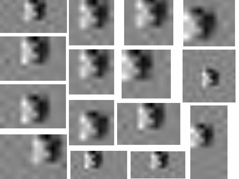
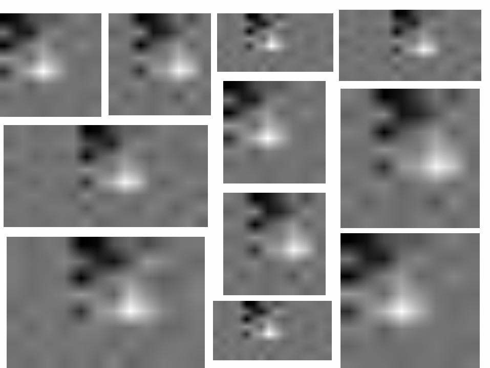
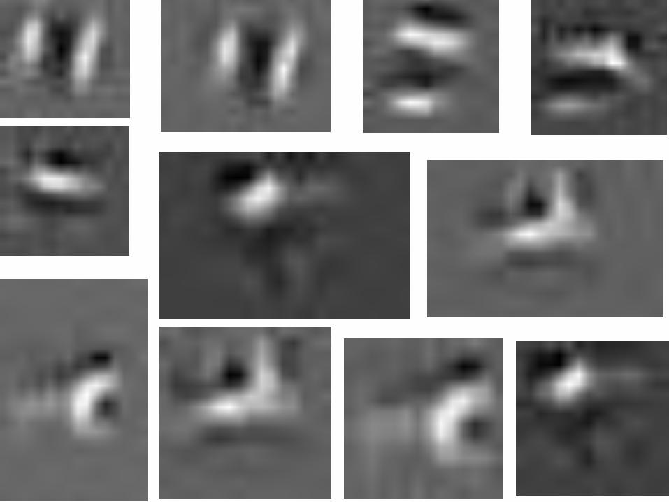
Receptive fields
• The pattern in the input image that each neuron sees is its “Receptive Field”
• The receptive field for a first layer neurons is simply its arrangement of weights
• For the higher level neurons, the actual receptive field is not immediately obvious and must be calculated– What patterns in the input do the neurons actually respond to?
– We estimate it by setting the output of the neuron to 1, and learning the input by backpropagation
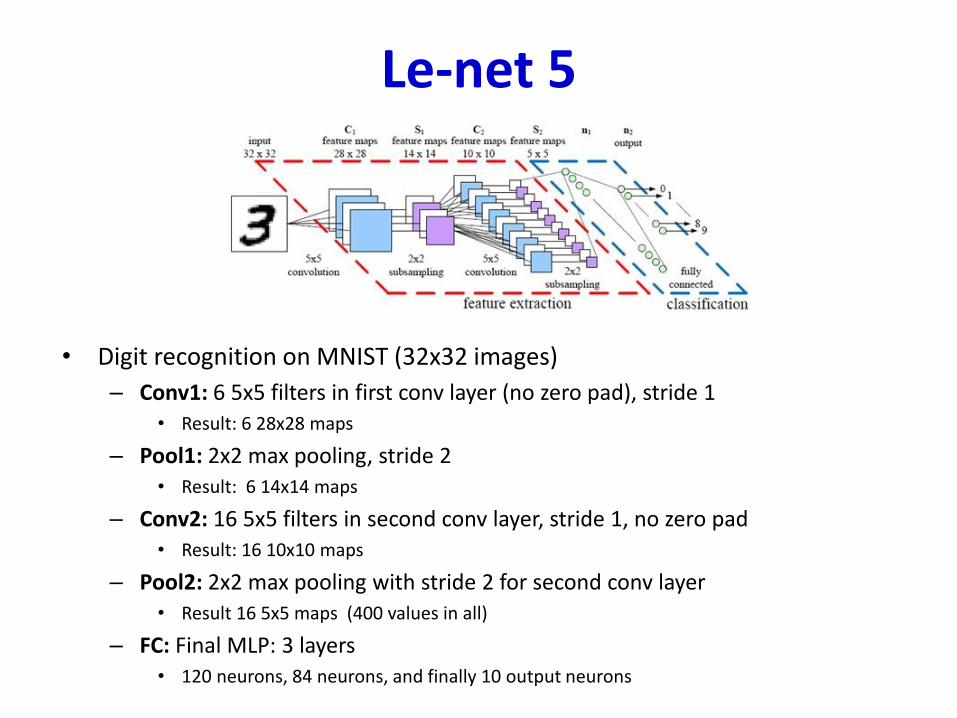
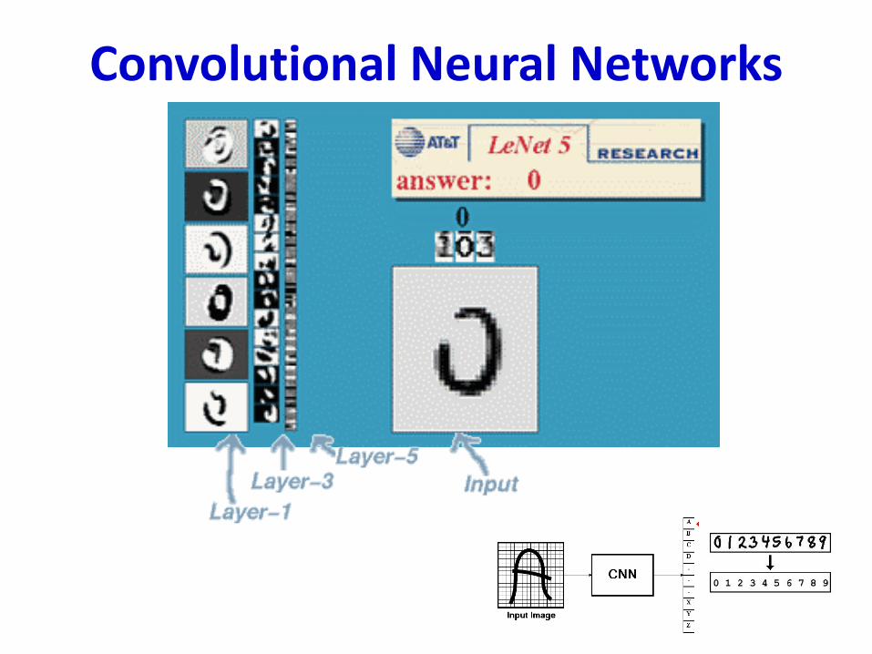
Le-net 5
• Digit recognition on MNIST (32x32 images)
– Conv1: 6 5x5 filters in first conv layer (no zero pad), stride 1• Result: 6 28x28 maps
– Pool1: 2x2 max pooling, stride 2• Result: 6 14x14 maps
– Conv2: 16 5x5 filters in second conv layer, stride 1, no zero pad• Result: 16 10x10 maps
– Pool2: 2x2 max pooling with stride 2 for second conv layer• Result 16 5x5 maps (400 values in all)
– FC: Final MLP: 3 layers• 120 neurons, 84 neurons, and finally 10 output neurons
Nice visual example
• http://cs.stanford.edu/people/karpathy/convnetjs/demo/cifar10.html
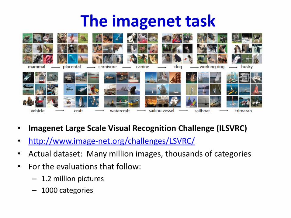
The imagenet task
• Imagenet Large Scale Visual Recognition Challenge (ILSVRC)
• http://www.image-net.org/challenges/LSVRC/
• Actual dataset: Many million images, thousands of categories
• For the evaluations that follow:
– 1.2 million pictures
– 1000 categories
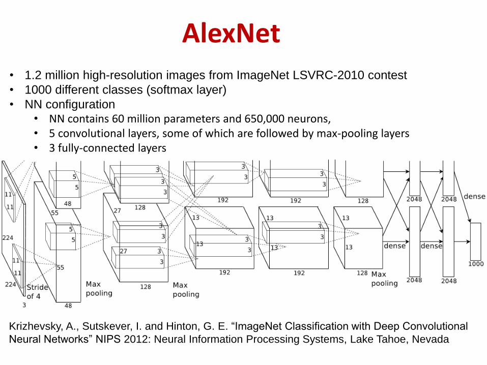
AlexNet• 1.2 million high-resolution images from ImageNet LSVRC-2010 contest
• 1000 different classes (softmax layer)
• NN configuration • NN contains 60 million parameters and 650,000 neurons, • 5 convolutional layers, some of which are followed by max-pooling layers• 3 fully-connected layers
Krizhevsky, A., Sutskever, I. and Hinton, G. E. “ImageNet Classification with Deep Convolutional
Neural Networks” NIPS 2012: Neural Information Processing Systems, Lake Tahoe, Nevada
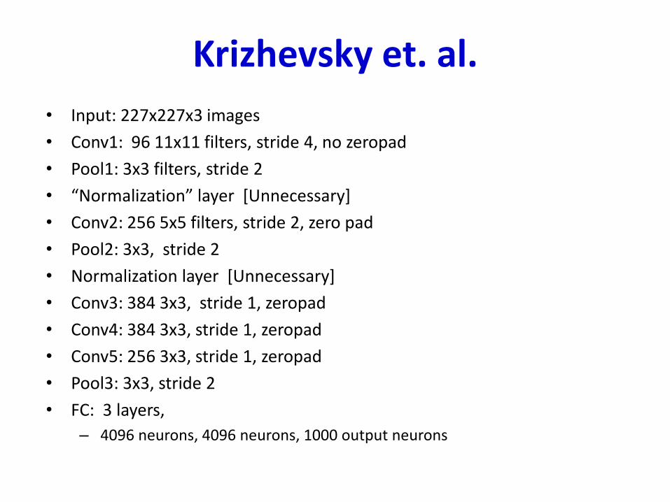
Krizhevsky et. al.
• Input: 227x227x3 images
• Conv1: 96 11x11 filters, stride 4, no zeropad
• Pool1: 3x3 filters, stride 2
• “Normalization” layer [Unnecessary]
• Conv2: 256 5x5 filters, stride 2, zero pad
• Pool2: 3x3, stride 2
• Normalization layer [Unnecessary]
• Conv3: 384 3x3, stride 1, zeropad
• Conv4: 384 3x3, stride 1, zeropad
• Conv5: 256 3x3, stride 1, zeropad
• Pool3: 3x3, stride 2
• FC: 3 layers,
– 4096 neurons, 4096 neurons, 1000 output neurons
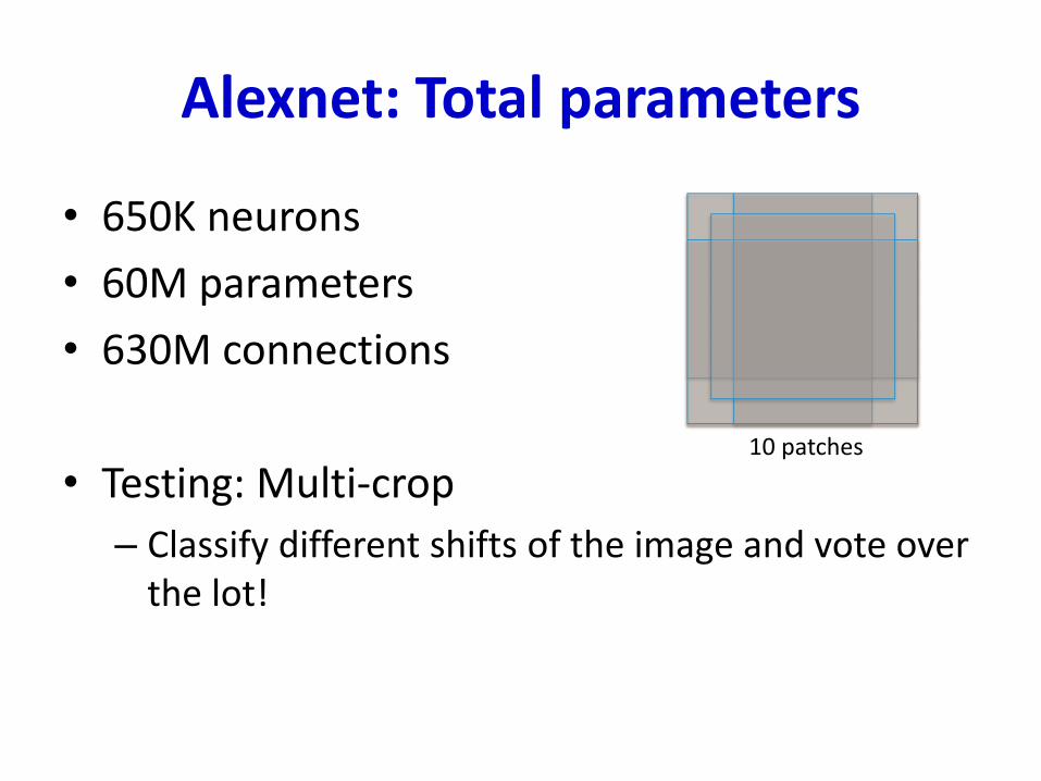
Alexnet: Total parameters
• 650K neurons
• 60M parameters
• 630M connections
• Testing: Multi-crop
– Classify different shifts of the image and vote over the lot!
10 patches
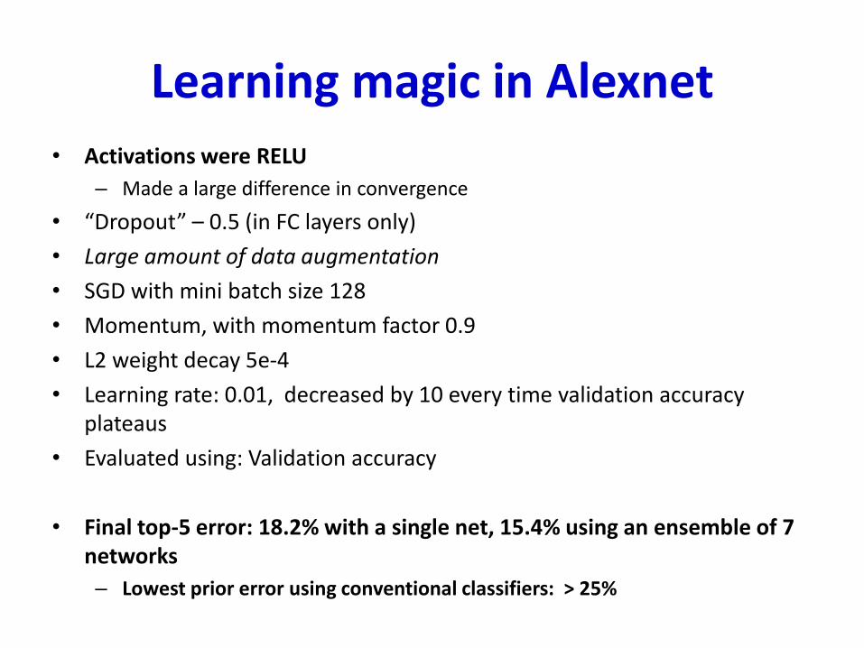
Learning magic in Alexnet• Activations were RELU
– Made a large difference in convergence
• “Dropout” – 0.5 (in FC layers only)
• Large amount of data augmentation
• SGD with mini batch size 128
• Momentum, with momentum factor 0.9
• L2 weight decay 5e-4
• Learning rate: 0.01, decreased by 10 every time validation accuracy plateaus
• Evaluated using: Validation accuracy
• Final top-5 error: 18.2% with a single net, 15.4% using an ensemble of 7 networks
– Lowest prior error using conventional classifiers: > 25%
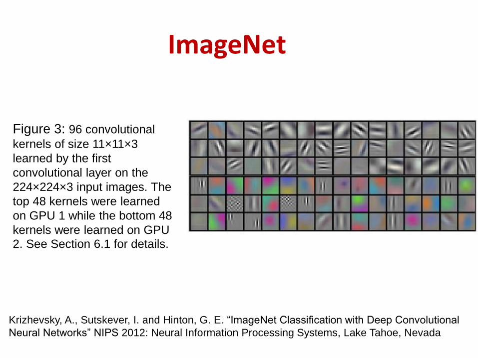
ImageNet
Figure 3: 96 convolutional
kernels of size 11×11×3
learned by the first
convolutional layer on the
224×224×3 input images. The
top 48 kernels were learned
on GPU 1 while the bottom 48
kernels were learned on GPU
2. See Section 6.1 for details.
Krizhevsky, A., Sutskever, I. and Hinton, G. E. “ImageNet Classification with Deep Convolutional
Neural Networks” NIPS 2012: Neural Information Processing Systems, Lake Tahoe, Nevada
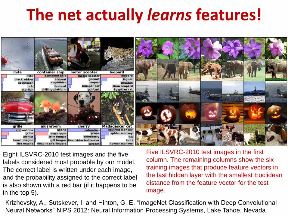
The net actually learns features!
Krizhevsky, A., Sutskever, I. and Hinton, G. E. “ImageNet Classification with Deep Convolutional
Neural Networks” NIPS 2012: Neural Information Processing Systems, Lake Tahoe, Nevada
Eight ILSVRC-2010 test images and the five
labels considered most probable by our model.
The correct label is written under each image,
and the probability assigned to the correct label
is also shown with a red bar (if it happens to be
in the top 5).
Five ILSVRC-2010 test images in the first
column. The remaining columns show the six
training images that produce feature vectors in
the last hidden layer with the smallest Euclidean
distance from the feature vector for the test
image.

ZFNet
• Zeiler and Fergus 2013
• Same as Alexnet except:– 7x7 input-layer filters with stride 2
– 3 conv layers are 512, 1024, 512
– Error went down from 15.4% 14.8%• Combining multiple models as before
5121024512
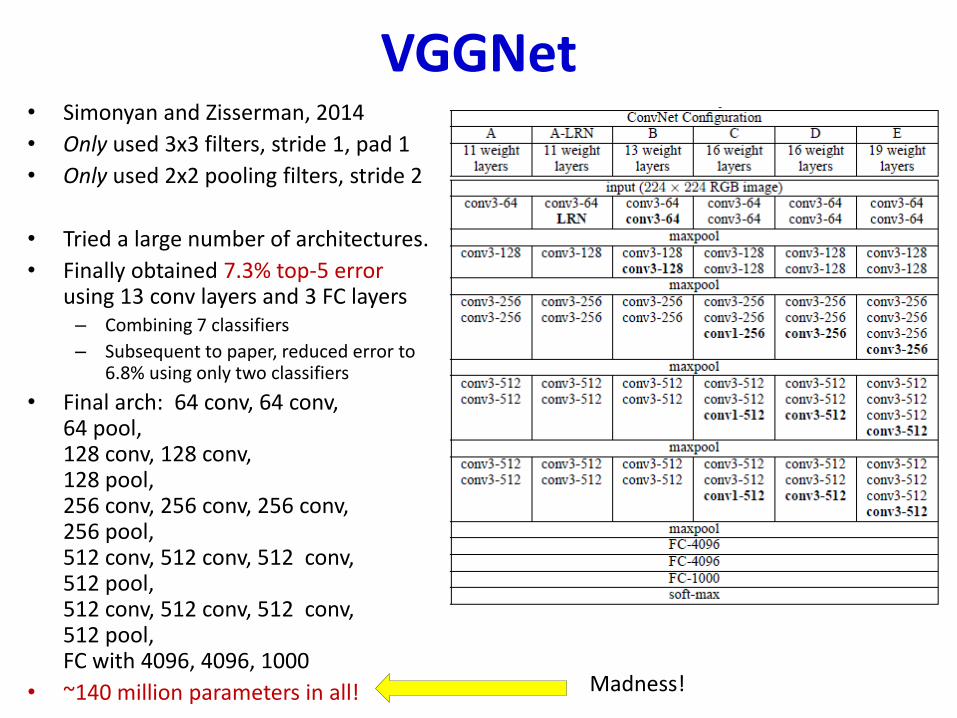
VGGNet• Simonyan and Zisserman, 2014
• Only used 3x3 filters, stride 1, pad 1
• Only used 2x2 pooling filters, stride 2
• Tried a large number of architectures.
• Finally obtained 7.3% top-5 error using 13 conv layers and 3 FC layers– Combining 7 classifiers
– Subsequent to paper, reduced error to 6.8% using only two classifiers
• Final arch: 64 conv, 64 conv, 64 pool, 128 conv, 128 conv, 128 pool,256 conv, 256 conv, 256 conv, 256 pool,512 conv, 512 conv, 512 conv, 512 pool,512 conv, 512 conv, 512 conv, 512 pool,FC with 4096, 4096, 1000
• ~140 million parameters in all! Madness!
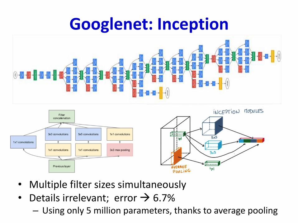
Googlenet: Inception
• Multiple filter sizes simultaneously• Details irrelevant; error 6.7%
– Using only 5 million parameters, thanks to average pooling
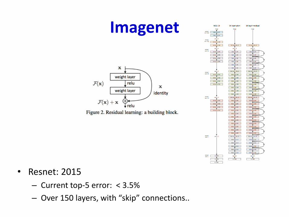
Imagenet
• Resnet: 2015
– Current top-5 error: < 3.5%
– Over 150 layers, with “skip” connections..
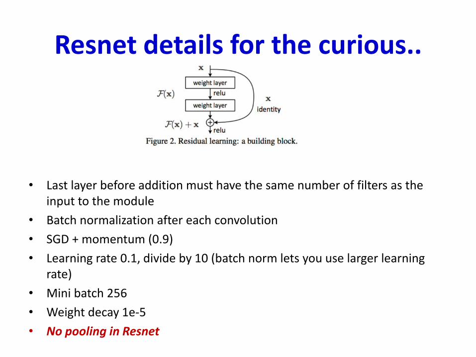
Resnet details for the curious..
• Last layer before addition must have the same number of filters as the input to the module
• Batch normalization after each convolution
• SGD + momentum (0.9)
• Learning rate 0.1, divide by 10 (batch norm lets you use larger learning rate)
• Mini batch 256
• Weight decay 1e-5
• No pooling in Resnet
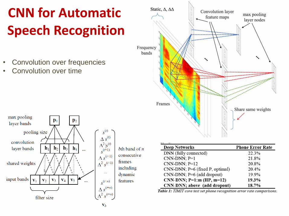
CNN for Automatic Speech Recognition
• Convolution over frequencies
• Convolution over time
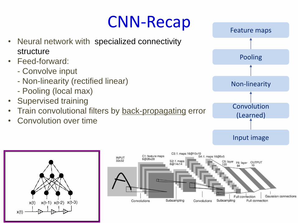
• Neural network with specialized connectivity
structure
• Feed-forward:
- Convolve input
- Non-linearity (rectified linear)
- Pooling (local max)
• Supervised training
• Train convolutional filters by back-propagating error
• Convolution over time
Feature maps
Pooling
Non-linearity
Convolution(Learned)
Input image
CNN-Recap