Working Paper Series Congressional Budget Office

Washington, D.C.

Does Government Debt Crowd Out Investment? A Bayesian DSGE Approach

Nora Traum Department of Economics

Indiana University Bloomington ntraum@indiana.edu

Shu-Chun Susan Yang Congressional Budget Office

sc.susan.yang@gmail.com

April 2010 2010-02

CBO’s Working and Technical Papers are preliminary and are circulated to stimulate discussion and critical comments. The papers are not subject to CBO’s formal review and editing process. The analysis and conclusions expressed are those of the authors and should not be interested as those of the Congressional Budget Office. References in publications should be cleared with authors. Papers in this series can be obtained from www.cbo.gov/pubications.

DOES GOVERNMENT DEBT CROWD OUT INVESTMENT?

A BAYESIAN DSGE APPROACH

NORA TRAUM AND SHU-CHUN S. YANG

Abstract. We estimate the crowding-out effects of government debt for the U.S. economyusing a New Keynesian model with a detailed fiscal specification. The estimation accountsfor the interaction between monetary and fiscal policies. Whether private investment iscrowded in or out in the short term depends on the fiscal or monetary shock that trig-gers debt expansion. Contrary to the conventional view of crowding out, no systematicrelationship among debt, the real interest rate, and investment exists. At longer horizons,distortionary financing is important for the negative investment response to a debt expan-sion.

Keywords: Crowding Out; Distortionary Debt Financing; Fiscal and Monetary Policy In-teractions; Bayesian Estimation

JEL Codes: C11; E63; H63

We thank Eric Leeper for his advice and support throughout the project. Also, we thank Robert Dennis,Eric Engen, Juan Carlos Escanciano, Jeffrey Kling, Joon Park, Todd Walker, and all seminar participants atIndiana University, the Congressional Budget Office, the Board of Governors, Princeton University, LondonBusiness School, University of Cincinnati, North Carolina State University, Wesleyan University, Universityof Arkansas, the International Monetary Fund, and Paris School of Economics for helpful comments. Theviews expressed in this paper are those of authors and should not be interpreted as those of the CongressionalBudget Office.

1. Introduction

The past decade in the United States has been a period of tremendous fiscal activity:

expenditures on the war on terrorism, two major tax cuts in 2001 and 2003, several fiscal

stimulus packages in 2008 and 2009, and the financial rescue programs. These activities

have occurred against a backdrop of demographic trends that suggest accelerated spending

increases in future medical programs and Social Security. The Congressional Budget Office

(2009) projects that federal debt in 2080 will reach 283 percent and 716 percent, respectively,

of GDP under the extended current-law scenario and an alternative fiscal scenario, suggesting

an unsustainable path for U.S. fiscal policy.1 The active use of fiscal policy has raised concern

about debt accumulation and rekindled a classic economic debate: Will government debt

accumulation lead to declines in (i.e. crowd out) private investment?

This paper estimates a dynamic stochastic general equilibrium (DSGE) model using

Bayesian methods to evaluate the extent of crowding out by government debt for the U.S.

economy. Several recent papers employ Bayesian techniques to understand the economic ef-

fects of fiscal policy. Most of them, however, have not fully modeled the interactions between

monetary and fiscal policy or fiscal adjustments induced by government debt accumulation

[Coenen and Straub (2005), Forni, Monteforte, and Sessa (2009), Lopez-Salido and Rabanal

(2006)]. Previous estimated DSGE models that account for monetary and fiscal policy in-

teractions, on the other hand, do not model distortionary taxes [for example, Leeper and

Sims (1994) and Kim (2000)]. Our model incorporates a rather detailed fiscal specification.

The rich dynamics between monetary and fiscal policy in the model, in turn, help explain

the investment response to government debt accumulation.

Following World War II, many economists were concerned about the impact of government

debt [for example, Domar (1944), Leland (1944), Lerner (1945), Wallich (1946), and the

references therein]. Since then, a conventional view has emerged, suggesting that government

1The alternative fiscal scenario incorporates some policy changes that have been regularly made in thepast and are widely expected to occur.

1

borrowing is expansionary in the short run but contractionary in the long run.2 Keynesian

economic theory argues that when prices and wages are sticky, higher debt caused by deficit-

financed tax cuts or spending increases adds to aggregate demand, leading income and output

to increase. The deficits, however, reduce public saving. Because private saving and capital

inflows may not increase enough to fully offset government borrowing, interest rates can

rise over time. Consequently, investment is crowded out, and capital and output eventually

decline, negating the short run expansionary benefits.

Building on this theoretical view, many empirical studies have estimated the reduced-form

relationship between government debt (or deficits) and interest rates at various horizons. A

positive estimated relationship between the two variables is viewed as evidence of crowding

out. Surveys of the literature generally conclude a lack of consensus among the findings.3 One

of the main contributions of this paper is to demonstrate, using an estimated DSGE model,

that even when government debt leads investment to fall, no systematic relationship between

debt and real interest rates exists. The result explains why empirical studies focusing on the

relationship between interest rates and debt are often inconclusive about the crowding out

effect of government debt.

We add fiscal details to a standard New Keynesian model that has been shown to fit

the data well [Del Negro, Schorfheide, Smets, and Wouters (2007) and Smets and Wouters

(2007)] and is used for monetary policy analysis. Most fiscal instruments can respond to

government indebtedness, as in Leeper, Plante, and Traum (2010). In addition, income tax

rates adjust automatically to the state of the economy, as does the income tax policy in

practice. Instead of assuming all government spending is wasteful, we distinguish between

2See Bernheim (1989) and Elmendorf and Mankiw (1999) for a detailed discussion.3See Elmendorf and Mankiw (1999), Gale and Orszag (2003), and Engen and Hubbard (2005). For a

survey of the earlier studies, see Barth, Iden, and Russek (1984) and Appendix A in The Economic Outlook,February [Congressional Budget Office (1984)]. Laubach (2009) finds a positive and significant relationshipbetween debt or deficits and interest rates when long-horizon forward rates and projected federal deficits areused. Engen and Hubbard (2005) also obtain similar results using the same measures for the two variables;however, they find that when the dependent variable is the change in the forward rate rather than the level,the positive coefficient is insignificant.

2

government consumption and productive government investment. Since the extent to which

consumers are myopic has received much attention in the debate of fiscal policy effects, we

include non-savers (also known as liquidity-constrained or rule-of-thumb agents) as well as

savers (the forward-looking agents with rational expectations), following Gali, Lopez-Salido,

and Valles (2007) and Forni, Monteforte, and Sessa (2009).4

A priori, the model does not impose restrictions on whether government debt crowds

out or in investment and on how government debt affects the economy. By estimating

most structural and policy parameters, we assess the importance of various factors—myopic

behaviors, fiscal interventions, debt financing, and monetary policy—for determining the

debt effects in the data.

Our estimation identifies several factors important in driving the investment response to

rising government debt: the source of policy changes that give rise to debt growth, the

responses of monetary policy, and distortionary debt financing. In the short run, the effect

of government debt is mainly determined by the type of fiscal or monetary policy shock

that triggers debt accumulation. Higher government debt can crowd in investment despite a

higher real interest rate if the debt is generated by a reduction in capital tax rates or by an

increase in productive government investment, because both raise the net return to capital.

This result is consistent with those from calibrated models, as in Ludvigson (1996) and

Leeper and Yang (2008), and Freedman, Kumhof, Laxton, Muir, and Mursala (2009). Over

a longer horizon, distortionary financing plays an important role in the negative investment

response following a debt expansion. The estimation finds most fiscal instruments respond

to debt systematically under rather diffuse priors: when the debt-to-output ratio rises, the

government reduces its purchases and transfers and increases income taxes to rein in debt

growth. Among the various instruments used for fiscal adjustments, raising income taxes,

4The debate concerns whether government debt is perceived as net wealth [Modigliani (1961), Barro(1974), Blanchard (1985), and Smetters (1999)]. If so, people behave myopically as non-savers in our model.

3

in particular the capital tax rate, has a strong negative impact on investment, as found by

Leeper, Plante, and Traum (2010) and Uhlig (2009) in neoclassical growth models.

We also find that monetary policy—in particular, the central bank’s responsiveness to

output—matters systematically for the path of investment. The more aggressively the cen-

tral bank responds to output fluctuations following a deficit-financed fiscal intervention, the

smaller the increase or the larger the decline in investment, depending on which fiscal instru-

ment triggers the debt expansion. In the case of a positive government investment shock, a

sufficiently large response in the nominal interest rate can reverse the crowding-in effect on

investment in the short run.

Finally, our estimation isolates historical fiscal innovations, which allows us to evaluate

the effects of individual fiscal policy episodes in our sample. We study the effects of the

1990s tax increases and the deficit-financed tax cuts during the recession in 2001 and 2002.

Counterfactual exercises find that when the capital and labor tax innovations from 1993Q1

to 1997Q2 are turned off, the real value of federal debt in 1997Q2 is 11 percent higher and

investment is 2 percent higher than their historical values, suggesting that fiscal adjust-

ments have a negative effect on investment. In addition, we find that the 2001 and 2002

tax cuts were expansionary, but monetary policy during the period played a bigger role in

counteracting the 2001 recession.

2. The Benchmark Model

The model is a conventional New Keynesian model based on Christiano, Eichenbaum,

and Evans (2005), Smets and Wouters (2007), Gali, Lopez-Salido, and Valles (2007), and

Forni, Monteforte, and Sessa (2009). We include two types of households: savers, who are

forward-looking with access to complete asset and capital markets, and non-savers, who do

not have access to financial or capital markets and consume all of their disposable income

each period. Because non-savers have a higher marginal propensity to consume than savers,4

their presence allows stronger short-run demand effects following expansionary fiscal policy

actions than in models with only savers. Non-savers also break Ricardian equivalence, so

lump-sum transfers are distortionary.

Other features of the model are standard in the New Keynesian literature. We incorporate

two real rigidities—variable capital utilization and investment adjustment costs—and two

nominal rigidities for prices and wages, both adjusting by a Calvo (1983) mechanism with

partial indexation to past inflation.5 The equilibrium system of the model is log-linearized

and solved by Sims’s (2001) algorithm. Appendix A describes the equilibrium.

2.1. Households. The economy is populated by a continuum of households on the interval

[0, 1], of which a fraction µ are non-savers and a fraction (1− µ) are savers. The superscript

S indicates a variable associated with savers and N with non-savers.

2.1.1. Savers. The household j ∈ [0, 1 − µ] maximizes its utility, given by

E0

∞∑

t=0

βtubt

[cSt (j)

1−γ − 1

1 − γ−LSt (j)

1+κ

1 + κ

], (1)

where β ∈ (0, 1) is the discount factor, γ ≥ 0 is the inverse of the intertemporal elasticity of

substitution, and κ ≥ 0 is the labor preference parameter. The economy has a continuum of

differentiated labor inputs indexed by l ∈ [0, 1]. We assume that each household supplies all

differentiated labor inputs to eliminate labor income discrepancies from individual households

supplying differentiated labor services, as in Schmitt-Grohe and Uribe (2004). The total

hours supplied by household j satisfies the constraint LSt (j) =∫ 1

0lSt (j, l)dl, where lSt (j, l)

is the amount of labor input l supplied by saver j. Hours are demand-driven, and each

household j works sufficient hours to meet the market demand for the chosen monopolistic

wage rates. The wage decisions are delegated to unions, which are discussed below.

5Habit formation, commonly included in DSGE models, is dropped from the specification. Because non-saver households react to most the fiscal shocks differently from savers, non-savers serve a function similarto habit formation for smoothing aggregate consumption.

5

The general preference shock ubt is assumed to follow an AR(1) process

ln(ubt) = ρb ln(ubt−1) + σbεbt , εbt ∼ N(0, 1), 0 < ρb < 1 . (2)

The flow budget constraint in units of consumption goods for saver j is given by

(1 − τLt )

∫ 1

0

Wt(l)

PtlSt (j, l)dl + (1 − τKt )

RKt vt(j)k

St−1(j)

Pt+Rt−1b

St−1(j)

πt+ zt(j) + dSt (j)

= cSt (j) +iSt (j)

1 + τCt+ bSt (j) , (3)

where τLt , τKt , and τCt are tax rates on labor income, capital income, and consumption, and

zt(j) represents lump-sum government transfers. Wt(l) is the nominal wage rate for labor

input l, and Pt is the general consumer price, inclusive of consumption taxes;∫ 1

0Wt(l)Pt

lSt (j, l)dl

is the total real labor income for household j. At time t, household j purchases bSt (j) units of

government debt, which paysRtb

St (j)

πt+1units of consumption goods at t+1, where πt+1 ≡

Pt+1

Ptis

the gross inflation rate for the consumer price index. dSt (j) is dividends received from profits

of the monopolistic firms, and iSt (j) is saver j’s gross investment. Note that introducing

consumption taxes causes a wedge between the producer price index, Pt, and the consumer

index, given by Pt = (1 + τ ct )Pt. We assume that no indirect taxes are paid on purchases of

investment goods, so that the price index of investment goods is the wholesale price Pt,6 as

in Forni, Monteforte, and Sessa (2009).

Savers control both the size of the capital stock kSt−1 and its utilization rate vt. A higher

utilization rate is associated with a higher depreciation rate of capital:

δ[vt(j)] = δ0 + δ1(vt (j) − 1) +δ22

(vt (j) − 1)2 , (4)

as in Schmitt-Grohe and Uribe (2008). We calibrate δ1 so that v = 1 in the steady state.

We define a new parameter ψ ∈ [0, 1) such that δ′′[1]

δ′ [1]

= δ2δ1

≡ ψ

1−ψ. RK

t is the nominal rental

rate for effective capital vt(j)kSt−1(j).

6Dividing the wholesale price index by the consumer price index leaves the tax wedge, which shows up in

the investment cost of iSt (j) in units of consumption goodsiS

t(j)

1+τc

t

.

6

The law of motion for private capital is given by

kSt (j) = (1 − δ[vt(j)])kSt−1(j) +

[1 − s

(uiti

St (j)

iSt−1(j)

)]× iSt (j) , (5)

where s(ui

tiSt (j)

iSt−1(j)

)× iSt (j) is investment the adjustment cost, as in Smets and Wouters (2003)

and Christiano, Eichenbaum, and Evans (2005). By assumption, s(1) = s′ (1) = 0, and

s′′ (1) ≡ s > 0 in the steady state. In addition, the adjustment cost is subject to an

investment-specific efficiency shock uit, which follows the AR(1) process

ln(uit) = ρi ln(uit−1) + σiεit, εit ∼ N(0, 1), 0 < ρi < 1 . (6)

2.1.2. Non-savers. Non-savers have the same preferences as savers, receive the same lump-

sum government transfers, and consume all their disposable income each period. The budget

constraint in units of consumption goods for the non-saver j ∈ (1 − µ, 1] is

cNt (j) = (1 − τLt )

∫ 1

0

Wt(l)

PtlNt (j, l)dl + zt(j) . (7)

2.2. Wage Setting and Labor Aggregation. To introduce wage rigidities, we assume

that monopolistic unions set the wages for the differentiated labor services, following Colciago

(2007) and Forni, Monteforte, and Sessa (2009). Households supply differentiated labor

inputs to a continuum of unions, indexed by l. Households are distributed uniformly across

the unions, implying that the aggregate demand for a specific labor input is spread uniformly

across all households. Therefore, in equilibrium the total hours worked for savers and non-

savers are equal: LSt (j) = LNt (j) =∫ 1

0lt (l) dl ≡ Lt.

A perfectly competitive labor packer purchases the differentiated labor inputs and assem-

bles them to produce a composite labor service Lt (sold to intermediate goods producing

firms) by the technology due to Dixit and Stiglitz (1977),

Lt =

[∫ 1

0

lt (l)1

1+ηwt dl

]1+ηwt

, (8)

where ηwt denotes a time-varying markup to wages that follows the exogenous AR(1) process

ln(ηwt ) = ρw ln(ηwt−1) + σwεwt , εwt ∼ N(0, 1), 0 < ρw < 1 . (9)

7

The demand function for a competitive labor packer can be derived from solving their

profit maximization problem subject to (8), which yields

lt (l) = Ldt

(Wt(l)

Wt

)−

1+ηwt

ηwt

, (10)

where Ldt is the demand for composite labor services, Wt is the aggregate wage, and1+ηw

t

ηwt

measures the elasticity of substitution between labor inputs.

In each period, a union receives a signal to reset its nominal wage with probability (1 − ωw).

Those who cannot reoptimize index their wages to past inflation according to the rule

Wt (l) = Wt−1 (l)πχw

t−1 , (11)

where χw ∈ [0, 1] introduces a backward looking component in the inflation process; that is,

the wage is indexed by χw percent of past inflation. Unions that receive the signal choose

the optimal nominal wage rate Wt (l) to maximize aggregate of households’ lifetime utility,

given by

Et

∞∑

i=0

(βωw)i{ubt+i

[(1 − µ)

(cSt+i)1−γ − 1

1 − γ+ µ

(cNt+i)1−γ − 1

1 − γ−L1+κt+i

1 + κ

]}, (12)

subject to four constraints: the aggregate budget constraints for savers and non-savers and

the individual and aggregate labor demand functions. Since hours worked are equal in

equilibrium, we drop the superscripts for savers and non-savers.

In a symmetric equilibrium, where Wt (l) = Wt, the nominal aggregate wage evolves

according to

Wt =

[(1 − ωw)W

−1

ηwt

t + ωw (πwt )−χw

ηwt W

−1

ηwt

t−1

]−ηw

t

, (13)

where πwt ≡ Wt

Wt−1is the gross wage inflation rate.

2.3. Firms and Price Setting. The production sector consists of intermediate and final

goods producing firms. A perfectly competitive final goods producer uses a continuum of

intermediate goods yt(i), where i ∈ [0, 1], to produce the final goods, Yt, according to the8

same constant-return-to-scale technology used by the labor packers,

[∫ 1

0

yt(i)1

1+ηpt di

]1+ηpt

≥ Yt , (14)

where ηpt denotes a time-varying markup to the intermediate goods’ prices that follows the

AR(1) process

ln(ηpt ) = ρp ln(ηpt−1) + σpεpt , εpt ∼ N(0, 1), 0 < ρp < 1 . (15)

We denote the price of the intermediate goods i as pt(i) and the price of final goods Yt as

Pt. The final goods producing firm chooses Yt and yt(i) to maximize profits subject to the

technology (14). The demand for yt(i) is given by

yt(i) = Yt

(pt(i)

Pt

)−

1+ηpt

ηpt

, (16)

where1+ηp

t

ηpt

is the elasticity of substitution between intermediate goods.

Intermediate goods producers, indexed by i, are monopolistic competitors in their product

market. Firm i produces by a Cobb-Douglas technology

yt(i) = uat (vtkt−1(i))α(lt(i))

1−α(KGt−1

)αG

, (17)

where α ∈ [0, 1], and αG ≥ 0 is the elasticity of output with respect to government capital

KGt−1. u

at denotes a covariance stationary technology shock, which evolves according to

ln(uat ) = ρa ln(uat−1) + σaεat , εat ∼ N(0, 1) . (18)

Analogous to labor unions, a monopolistic intermediate firm has a probability of (1 − ωp)

each period to reset its price. Firms that cannot reset optimally index their prices to past

inflation according to the rule

pt(i) = pt−1(i)πχp

t−1 . (19)9

Firms that can reset optimally choose their price pt(i) to maximize the expected sum of

discounted future real profits:

maxpt(i)

Et

∞∑

j=0

(ωpβ)jλSt+jλSt

Yt+j

[(pt(i)

Pt

) j∏

k=1

(πχ

p

t+k−1

πt+k

)]− 1+ηpt

ηpt

{(pt(i)

Pt

) j∏

k=1

πχp

t+k−1

πt+k−MCt+j

P t+j

}.

(20)

In a symmetric equilibrium, where pt (i) = pt, the producer price index Pt evolves according

to

Pt =

[(1 − ωp)p

−1

ηptt + ωpπ

−χp

ηpt

t P−1

ηpt

t−1

]−η

pt

. (21)

2.4. Monetary Policy. The monetary authority follows a Taylor-type rule, in which the

nominal interest rate Rt responds to its lagged value, the current inflation rate, and current

output. We denote a variable in percentage deviations from the steady state by a caret, as

in Rt. Specifically, the interest rate is set according to

Rt = ρrRt−1 + (1 − ρr)[φππt + φyYt

]+ σmεmt , εmt ∼ N(0, 1) . (22)

2.5. Fiscal Policy. Each period the government collects tax revenues and issues one-period

nominal bonds to finance its interest payments and expenditures, which include government

consumption GCt , government investment GI

t , and transfer payments to the households. The

flow budget constraint in units of consumption goods is

Bt + τKtRKt

PtvtKt−1 + τLt

Wt

PtLt +

τCt1 + τCt

Ct =Rt−1Bt−1

πt+GC

t +GIt + Zt . (23)

We assume that government investment can be productive. The law of motion for government

capital is given by

KGt =

(1 − δG

)KGt−1 +GI

t . (24)

Fiscal variables respond to the state of the economy according to the following rules:

τKt = ρK τKt−1 + (1 − ρK)

(ϕK Yt + γK s

bt−1

)+ σKε

Kt + φKLσLε

Lt , (25)

τLt = ρLτLt−1 + (1 − ρL)

(ϕLYt + γLs

bt−1

)+ σLε

Lt + φKLσKε

Kt , (26)

GCt = ρGCG

Ct−1 − (1 − ρGC)γGC s

bt−1 + σGCε

GCt , (27)

10

GIt = ρGIG

It−1 − (1 − ρGI)γGI s

bt−1 + σGIε

GIt , (28)

Zt = ρZ Zt−1 − (1 − ρZ)γZ sbt−1 + σZε

Zt , (29)

τCt = ρC τCt−1 + σCε

Ct , (30)

where sbt−1 ≡Bt−1

Yt−1, and εst ∼ i.i.d. N(0, 1) for s = {K, L, GC, GI, C, Z}.

When the debt-to-output ratio rises above its steady state level, the government can

adjust income taxes, government consumption and investment, or transfers to stabilize debt

growth. Among the general equilibrium studies with government debt, the vast majority

allow for a limited set of fiscal instruments to ensure fiscal solvency. For example, Erceg,

Guerrieri, and Gust (2005), Coenen and Straub (2005), and Ratto, Roeger, and in’t Veld

(2009) allow only lump-sum taxes to respond to debt. Kumhof and Laxton (2007) have

several instruments respond to debt but leave out capital taxes. Forni, Monteforte, and Sessa

(2009), Lopez-Salido and Rabanal (2006), Iwata (2009), and Zubairy (2009) allow for taxes

but not government spending to respond to debt. Leeper, Plante, and Traum (2010) find

that in the U.S. postwar data, labor and capital taxes, government spending, and transfers

all play a role in controlling debt growth. Thus, we allow for all these instruments to respond

to debt, except the consumption tax. In our data set, consumption taxes consist of federal

excise taxes and custom duties, which have an average share of GDP less than one percent.

To capture the role of income taxes as automatic stabilizers, capital and labor taxes are

allowed to respond to output contemporaneously (ϕK , ϕL ≥ 0). Because changes in income

tax codes often involve changes in labor and capital taxes simultaneously, we also allow an

unexpected exogenous movement in one tax rate to affect the other rate, as captured by φKL

in (25) and (26).

2.6. Aggregation. We denote the aggregate quantity of a variable xt by its capital letter

Xt. Aggregate consumption is given by

Ct =

∫ 1

0

ct(j)dj = (1 − µ)cSt + µcNt .

11

Lump-sum transfers are assumed to be identical across households, implying that

Zt =

∫ 1

0

zt(j)dj = zt .

Because only savers have access to the asset and capital markets, aggregate bonds, private

capital, investment, and dividends are

Bt =

∫ 1

0

bt(j)dj = (1 − µ)bSt , Kt =

∫ 1

0

kt(j)dj = (1 − µ)kSt ,

It =

∫ 1

0

it(j)dj = (1 − µ)iSt , Dt =

∫ 1

0

dt(j)dj = (1 − µ)dSt .

Finally, the goods market clearing condition is

Yt = Ct + It +GCt +GI

t . (31)

3. Estimation

The model is estimated with U.S. quarterly data from 1983Q1 to 2008Q1 using Bayesian

inference methods. The choice of the sample period is driven by two stability considerations:

(1) monetary policy is thought to be characterized by a Taylor rule [Taylor (1993)] over this

period; and (2) on average, monetary policy is thought to have been active and fiscal policy

passive (in the sense of Leeper (1991)).7

7When a longer sample is used, regime-switching between active and passive monetary and fiscal policiesis a more pronounced issue. Davig and Leeper (2006) find evidence for regime-switching in the postwar U.S.data. Because the monetary and fiscal policy rules we estimate are assumed to have constant coefficients forinflation and debt, we select a sample period where, on average, monetary policy is active and fiscal policyis passive.

12

We estimate the model using 12 observables, including real aggregate consumption, in-

vestment, labor, wages, the nominal interest rate, the gross inflation rate, and fiscal vari-

ables—capital, labor, and consumption tax revenues, real government consumption and in-

vestment, and transfers.8 Although the literature typically uses fiscal variables of all gov-

ernments, our fiscal variables are for the federal government only. Because state and local

governments generally have balanced-budget rules of various forms, fiscal financing decisions

are likely to differ across federal and state and local governments, and we only consider

modeling the former. Appendix B provides a detailed description of the data. We detrend

the logarithm of each time series with its own linear trend, except for the nominal interest

rate, which is detrended by the trend in inflation.9

We assume that the parameters are drawn independently, so that the joint distribution of

the parameters, p(θ), is simply the product of the marginal distributions. Given the plausible

interactions between monetary and fiscal policies, p(θ) has a non-zero density outside the

determinacy region of the parameter space. We restrict the parameter space to the subspace

in which the model has a unique rational expectations equilibrium. We denote this subspace

as ΘD and let I{θ ∈ ΘD} be an indicator function that is one if θ is in the determinacy

region and zero otherwise. Thus, our joint prior distribution is defined as

p(θ) =1

cp(θ)I{θ ∈ ΘD}, where c =

∫

θ∈ΘD

p(θ)dθ .

The equilibrium system of the model is written in a state-space form, where observables

are linked with other variables in the model. For a given set of structural parameters, we

8By not including debt, the invertibility test in Fernandez-Villaverde, Rubio-Ramirez, Sargent, and Wat-son (2007) fails. However, posterior mode estimation based on simulated data shows that our observables canrecover true parameters well. If we include debt as an observable, then one fiscal variable must be droppedto avoid singularity. This makes us unable to identify the standard deviation of the dropped fiscal variable,which further prevents us from conducting historical decompositions later.

9There is no consensus in the literature on a detrending method (see Canova (2009) for a discussion ofthe advantages and disadvantages of various detrending methods). An alternative approach is to match thedemeaned data to its model counterparts by allowing some shocks to be nonstationary. Incorporating suchfeatures into a model with fiscal policy is nontrivial, since several fiscal variables appear to have their owntrends. In addition, it is unclear which non-fiscal shocks should be modeled as nonstationary, as various oneshave been proposed as candidates to better match the data (see Greenwood, Hercowitz, and Krusell (1997),Greenwood, Hercowitz, and Krusell (2000), and Chang, Doh, and Schorfheide (2007)).

13

compute the value for the log posterior function, which combines the likelihood of the data,

L(y|θ), with the probability values of the parameters given the prior distributions. The

posterior is proportional to

p(Y |θ) ∝ L(y|θ)p(θ) .

The minimization routine csminwel by Christopher Sims is used to search for the set of

structural parameters that minimize the negative log posterior function. To check whether

multiple modes exist, we initiate the search for the posterior mode from 50 initial values.

The results suggest that multiple modes are not a major concern.10 Next, we construct

the posterior distribution using the random walk Metropolis-Hastings algorithm. Finally,

diagnostic tests are performed to ensure the convergence of the MCMC chain.11

3.1. Prior Distributions. We impose dogmatic priors over several parameters that are

hard to identify from the data. The discount factor, β, is set to 0.99, which implies an

annual steady-state real interest rate of 4 percent. The capital income share of total output,

α, is set to 0.36, implying a labor income share of 0.64. The quarterly depreciation rate for

private capital, δ0, is set to 0.025 so that the annual depreciation rate is 10 percent. We set

δG = 0.02, comparable to the calibrated value in DSGE models with productive investment

[Baxter and King (1993) and Kamps (2004)]. We assume that the steady state elasticity

of substitution in the goods and labor market ((1 + ηp)/ηp, (1 + ηw)/ηw) is 8, implying

the steady-state markups in the product and labor markets are approximately 14 percent.

This is consistent with evidence that the average price markup of U.S. firms is around 10-15

percent [Basu and Fernald (1995)]. Since there appears to be no consensus in the literature

10Forty searches converged to the same values, seven searches were cases where the numerical optimiza-tion procedure failed to converge, and the remaining three converged to values with much lower likelihoodnumbers.

11Because the MH algorithm is initialized with the estimated mode and Hessian, we check the gradientand the conditioning number of the Hessian at the mode and plot slices of the likelihood around the mode.We sample one million draws from the posterior distribution and discard the first 20,000 draws. The sampleis thinned by every 20 draws. A step size of 0.3 yields an acceptance ratio of 0.307. Diagnostic tests forconvergence include drawing trace plots, verifying whether the chain is well mixed, and performing Geweke’s((2005), pp. 149-150) Separated Partial Means test. Results are available upon request.

14

for the average markup in the U.S. labor market, we pick the same value for ηw by symmetry.

The steady-state inflation rate, π, is assumed to be 1.

The elasticity of output to government capital, αG, cannot be identified without informa-

tion about the capital stocks. The empirical literature has a wide range of values for αG,

ranging from a small negative number [Evans and Karras (1994)], to zero [Kamps (2004)],

to near 0.4 [Pereira and de Frutos (1999)]. For the baseline estimation, we make a conser-

vative assumption on the productivess of public capital and calibrate αG = 0.05. Sensitivity

analysis explores two alternative cases where αG = 0 and αG = 0.1. We find that the data

cannot distinguish between the three values for αG (see Table 3), as the log marginal data

densities in the three cases are virtually identical.

The rest of the calibrated parameters are steady-state fiscal variables computed from the

means of our data sample: The federal government consumption to output share is 0.070,

the federal government investment to output share is 0.004, the federal debt to annualized

output share is 0.386, the average marginal federal labor tax rate is 0.209, the capital tax

rate is 0.196, and finally, the consumption tax rate is 0.015. When computing these shares,

we use an output measure that is consistent with our model specification—namely, the sum

of consumption, investment, and total government purchases.

Columns 2, 3, and 4 in Table 1 list the prior distributions for all estimated parameters.

Our priors are similar to those in Smets and Wouters (2007) for the parameters found in

both models. The domains cover a range of values estimated by previous studies (see Smets

and Wouters (2003) and (2007) for a review of previous estimates).

A parameter less encountered in the literature is the share of non-savers, µ. Forni, Mon-

teforte, and Sessa (2009) and Iwata (2009) center the prior at 0.5 but obtain an estimate

around 0.35. Lopez-Salido and Rabanal’s (2006) estimate using U.S. data over a similar

sample period is between 0.10 to 0.39. Based on this information, we choose a beta prior

with a mean of 0.3 and standard deviation equal to 0.1.

15

The priors for the fiscal parameters were chosen to be fairly diffuse and cover a reason-

ably large range of the parameter space. To stabilize debt as a share of output, government

spending and transfers should respond negatively to a debt increase, and taxes should re-

spond positively. We assume normal distributions for the fiscal instruments’ responses to

debt (γGC , γGI , γK , γL, and γZ) with a mean of 0.15 and standard deviation of 0.1. While

these priors place a larger probability mass in the regions of expected signs, a small proba-

bility is allowed for the opposite signs. Our guidance to determine the prior range for the

γ’s is based on two considerations. First, when the γ’s are too high, overshooting occurs,

resulting in oscillation patterns that are not observed in the data. Second, when the γ’s are

too low, under active monetary policy, there does not exist an equilibrium. As capital and

labor taxes are progressive in the tax code, we restrict ϕK and ϕL to be positive, following

a gamma distribution. Since we incorporate Social Security taxes in our labor tax revenues,

the labor tax rate elasticity is expected to be a value below the capital tax rate elasticity

(since Social Security contributions have a cap and are regressive). The parameter measuring

the co-movement between capital and labor tax rates (σKL) is assumed to have a normal

distribution with a mean of 0.2 and a standard deviation of 0.1. The domain covers the

range of past estimates for this parameter [see Leeper, Plante, and Traum (2010) and Yang

(2005)].

A priori, our model does not impose restrictions on whether government debt crowds

out investment or crowds it in. Table 2 quantifies the extent of crowding out based on

30,000 draws from the prior and posterior distributions. It records the percentage of draws

that lead investment to be crowded out on impact of various fiscal shocks. Except for

government consumption and transfer increases, the priors can deliver positive or negative

investment responses following expansionary fiscal policy shocks. The table also reports the

5th and 95th cumulative present-value investment multipliers generated from the prior draws

following various fiscal shocks.12 With the exception of a government investment increase or

12 Investment multipliers are defined as the present-value sum of investment changes in levels divided bythe present-value sum of changes in a fiscal variable. Depending on the fiscal shock that triggers debt growth,

16

consumption tax decrease, the priors allow the 90 percent interval of investment multipliers

to cover both signs. In addition, even though the present-value investment multipliers for

government investment are positive and for consumption taxes are negative, on impact the

priors do not restrict the sign of the investment response. Thus, in these cases (as well as the

others) the model allows for the longer-term dynamics to vary qualitatively from the short-

run dynamics. Section 4 explore the economics of both short-run and longer-run responses

to expansionary fiscal shocks.

3.2. Posterior Estimates. The last four columns of table 1 provide the mode, mean, and

5th and 95th percentiles from the posterior distributions. Appendix C contains plots of the

priors against the posterior distributions. The plots suggest that the data contain infor-

mation for identifying most parameters. The labor preference parameter, κ, appears to be

weakly identified, as do the responses of tax rates to contemporaneous output, ϕK and ϕL.13

Model comparison results between the benchmark model and an alternative specification

where ϕK = ϕL = 0 indicate that the data cannot distinguish between the two specifications

(see Table 3).

Overall, the estimates for the common parameters in New Keynesian models are compara-

ble to others estimated with postwar U.S. data [Smets and Wouters (2007) and Fernandez-

Villaverde, Guerron-Quintana, and Rubio-Ramirez (2010)]. Our estimate of risk aversion

parameter is much bigger than the values estimated or calibrated in previous studies, imply-

ing an intertemporal elasticity of substitution of 0.37.14 The mean estimate of κ implies that

the Frisch labor elasticity is 0.48, a value within the range of the findings of micro studies

[Browning, Hansen, and Heckman (1999)].

the denominator can be changes in capital, labor, or consumption tax revenues, government consumptionor investment, or transfers. The sums are over 1000 quarters, and present values are discounted by themodel-implied interest rate path.

13A singular value decomposition of the Fisher information matrix of the likelihood at various parametercombinations suggests that κ is the most weakly identified parameter in the model.

14The literature has a wide range of estimates for this parameter [Guvenen (2006)].17

The mean long-run response of the nominal interest rate to inflation is consistent with

recent estimates. The mean response to output is similar to Taylor’s (1993) estimate. We

also find evidence of a substantial degree of interest rate smoothing, consistent with the

literature on estimated interest rate rules. The rest of this section discusses parameters less

frequently encountered in the literature and how well the model fits the data.

3.2.1. Fraction of non-savers. The mean estimate for the fraction of non-savers µ is 0.18,

and 5th and 95th percentiles are [0.10, 0.27]. The relatively low fraction of non-savers sug-

gests the importance of forward-looking behavior in explaining the aggregate effects of fiscal

policy. Although myopic behavior has been important in explaining fiscal policy effects in

the literature since Mankiw (2000) and Gali, Lopez-Salido, and Valles (2007), our mean es-

timate is much smaller than the commonly calibrated value of 0.5, based on single-equation

estimation of a consumption function [Campbell and Mankiw (1989) and Gali, Lopez-Salido,

and Valles (2007)]. Previous studies have incorporated non-savers into models so that ag-

gregate consumption can increase following a positive government spending shock. Given

the mean estimates for the benchmark model, our model requires a fraction of 0.45 in order

to deliver a positive short-term consumption response to an increase in government con-

sumption, which falls outside the 90-percent interval. Our results are consistent with vector

autoregression (VAR) estimates.15 VARs with either federal government consumption alone

or the sum of federal government consumption and investment find that, for our sample

period (1983Q1 to 2008Q1), an increase in government spending does not have a positive

effect on consumption.16

15The evidence of the positive consumption response following a government spending shock found inthe literature [e.g. Gali, Lopez-Salido, and Valles (2007) and Bouakez and Rebei (2007)] is based on alonger postwar U.S. sample. VARs based on smaller samples (Perotti (2005) and Bilbiie, Meier, and Mueller(forthcoming)) find a muted consumption response.

16The VARs are ordered with government spending first, followed by GDP, consumption, and investment.Identification is achieved using a Cholesky decomposition. When consumption excludes durables, investmentis defined as the sum of gross private domestic investment and durables.

18

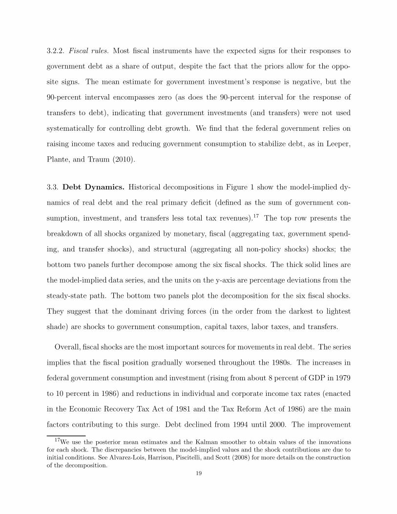
3.2.2. Fiscal rules. Most fiscal instruments have the expected signs for their responses to

government debt as a share of output, despite the fact that the priors allow for the oppo-

site signs. The mean estimate for government investment’s response is negative, but the

90-percent interval encompasses zero (as does the 90-percent interval for the response of

transfers to debt), indicating that government investments (and transfers) were not used

systematically for controlling debt growth. We find that the federal government relies on

raising income taxes and reducing government consumption to stabilize debt, as in Leeper,

Plante, and Traum (2010).

3.3. Debt Dynamics. Historical decompositions in Figure 1 show the model-implied dy-

namics of real debt and the real primary deficit (defined as the sum of government con-

sumption, investment, and transfers less total tax revenues).17 The top row presents the

breakdown of all shocks organized by monetary, fiscal (aggregating tax, government spend-

ing, and transfer shocks), and structural (aggregating all non-policy shocks) shocks; the

bottom two panels further decompose among the six fiscal shocks. The thick solid lines are

the model-implied data series, and the units on the y-axis are percentage deviations from the

steady-state path. The bottom two panels plot the decomposition for the six fiscal shocks.

They suggest that the dominant driving forces (in the order from the darkest to lightest

shade) are shocks to government consumption, capital taxes, labor taxes, and transfers.

Overall, fiscal shocks are the most important sources for movements in real debt. The series

implies that the fiscal position gradually worsened throughout the 1980s. The increases in

federal government consumption and investment (rising from about 8 percent of GDP in 1979

to 10 percent in 1986) and reductions in individual and corporate income tax rates (enacted

in the Economic Recovery Tax Act of 1981 and the Tax Reform Act of 1986) are the main

factors contributing to this surge. Debt declined from 1994 until 2000. The improvement

17We use the posterior mean estimates and the Kalman smoother to obtain values of the innovationsfor each shock. The discrepancies between the model-implied values and the shock contributions are due toinitial conditions. See Alvarez-Lois, Harrison, Piscitelli, and Scott (2008) for more details on the constructionof the decomposition.

19

was mainly due to an increase in individual income tax rates on the relatively high income

brackets (enacted in the Omnibus Budget Reconciliation Act of 1993) and a decrease in

federal spending (falling from 9 percent in 1990 to about 6 percent in the late 1990s). The

model-implied deficit series experiences a small spike in 1991, moving from above the trend

to below the trend in the first quarter of 1991 before continuing to further increase above the

trend until approximately 1993. This corresponds with the Omnibus Budget Reconciliation

Act of 1990’s enactment to increase the highest income tax rates, which became effective

January 1, 1991.

In addition to fiscal shocks, monetary policy shocks also play an important role in real

debt movements. The top row of Figure 1 shows that monetary policy shocks often offset

some of the fiscal shocks’ impact on debt or the primary deficit. During the boom in the

1990s, monetary policy became relatively tight starting in late 1994. A positive interest

rate shock drove up the real value of debt by lowering the price level and increasing interest

rate payments. Analogously, when the federal funds rate was gradually lowered during the

economic downturn in early 2000s, monetary policy contributed to lowering the real value

of debt.

4. Crowding Out By Government Debt

Fiscal and monetary shocks are the main driving forces for the real value of U.S. govern-

ment debt in the post-1983 sample. This section investigates the economics underlying the

links between investment and government debt, focusing on the debt changes driven by fiscal

and monetary policy shocks.

We first examine the model implied Tobin’s q [Tobin (1969)]. Define qt ≡ξt(1+τC

t )λS

t

, where

λSt and ξt are the Lagrangian multipliers for the constraints (3) and (5) in the savers’ utility

optimization problem. qt has the interpretation of the shadow price of increasing capital at

the end of t by one unit. Investment tends to rise with qt. The log-linearized expression of20

Tobin’s q from its steady state is

qt =τC

1 + τCτCt − (Rt −Etπt+1) + β(1 + τC)(1 − τK)rKEtr

Kt+1 (32)

−[τKrKβ

(1 + τC

)]Etτ

Kt+1 + β(1− δ)Etqt+1 −

βτC(1 − δ)

(1 + τC)Etτ

Ct+1 ,

where rKt ≡RK

t

Ptis the real rate of return for private capital.

Consistent with the conventional view, the negative coefficient on the real interest rate

(Rt − Etπt+1) indicates that a higher real rate discourages investment. Equation (4) also

points out that investment decisions are influenced by several other factors. A higher ex-

pected real return on capital makes agents want to invest more, but a higher expected

capital tax rate does the opposite. In the model, the consumption tax shock serves as a

relative price shock between consumption and investment, because consumption taxes are

levied only on consumption goods. An increase in the consumption tax signals a fall in the

price of investment goods relative to consumption goods. In contrast, expectations of future

cheaper investment goods, through an expected increase in the future consumption tax rate,

delay investment decisions. Finally, the higher expected shadow price indicates that capital

is more valuable in the future, so it encourages current investment. Next, we examine how

fiscal and monetary shocks affect investment decisions.

4.1. Fiscal Policy and Crowding Out. When a fiscal shock hits the economy, it has a

direct effect on the evolution of variables from the shock itself and a secondary effect through

future debt financing. Delayed financing causes government debt to accumulate, which brings

forth future policy adjustments that can affect both the current economy (through policy

expectations) and the future economy (through the implementation of policy adjustments).

We first look at the relationship between debt and investment implied by the overall effect

of a fiscal policy shock. Later we contrast the results with the net effect from debt financing.

Figures 2 and 3 show one standard deviation impulse responses to all policy shocks. The

solid lines are the responses under the posterior mean estimates. The dotted-dashed lines21

give the 5th and 95th percentiles based on the posterior distributions. The y-axis measures

percentage deviation from the steady state, and the x-axis denotes the number of years after

a shock.

Although all the expansionary fiscal shocks cause government debt to grow, investment

can rise or fall, depending on the type of shock. When government investment is increased or

the capital tax rate is decreased, higher debt is associated with higher investment, as shown

by the solid lines in the second and third columns of Figure 2. An increases in productive

government investment implies a higher stock of future public capital, which raises the

marginal product of private capital. Similarly, a reduction in the capital tax rate directly

increases the after-tax rate of return for investment. Because the tax shock is persistent,

this lowers expectations of future capital tax rates. Under either circumstance, investment

can rise as suggested by equation (4). In the conventional view, crowding out results from

decreases in national saving, which drives up the real interest rate and lowers investment.

We see that if a debt expansion is due to an increase in government investment or a decrease

in the capital tax rate, the higher expected return to capital or the lower expected capital

tax rate causes investment to rise despite a higher interest rate.

When labor or consumption tax rates decrease (the first and second columns of Figure

3), the probability intervals allow for investment to be crowded in or out in the short run.

A negative labor tax shock increases labor demand, which drives up the marginal product

of capital, and hence makes agents want to invest more. However, the debt-financed labor

tax cut induces policy adjustments, which involve higher capital and labor tax rates and

lower government spending. Under most combinations of fiscal adjustments drawn from the

posterior distributions, investment falls. For the reduction in the consumption tax rate, the

direct effect is a reduction in investment as investment goods become more expensive than

consumption goods. The initial positive response of investment is driven by the monetary

authority’s interest rate response: the more aggressively the monetary authority stabilizes

22

prices (following the decrease in the consumer’s price level), the more the real interest rate

declines, which drives up investment.

Among the six fiscal shocks, the only two shocks that produce debt effects largely consistent

with the conventional view are government consumption and transfers shocks. The first

column of Figure 2 shows that following an increase in government consumption, the real

interest rate rises and investment falls. When the government absorbs a larger share of goods,

it leaves the private sector with fewer goods to invest. As goods become more valuable,

the real interest rate rises to clear the goods market. A similar pattern is also observed

with the transfer shock (the third column of Figure 3). Rising transfers increase aggregate

consumption because non-savers consume more due to higher disposable income. Higher

demand for goods drives up the real interest rate, discouraging investment. Although the

real interest rate rises most of the time for either shock, it can be negative initially. Because

higher demand leads to higher prices and inflation expectations, the real interest rate (the

nominal rate less inflation expectations) can fall initially if prices are less sluggish to adjust.

The above discussion shows that a debt expansion need not lead the real interest rate to

rise and investment to fall. The relationships among these variables depend on which fiscal

innovation triggers the debt growth.

4.1.1. Distortionary debt financing. One important channel in which government debt can

affect the economy is through policy adjustments necessary to stabilize debt growth. To

understand the effects of distortionary debt financing, we construct a hypothetical economy

that is identical to the benchmark economy except for the manner in which government debt

is financed. In the hypothetical economy, the government follows a balanced budget rule,

and γGC = γGI = γK = γL = γZ = 0. We introduce a new lump-sum tax Xt on savers, which

shows up only in the savers’ budget constraints, and evolves to satisfy

Xt = GCt +GI

t + Zt − τKtRKt

PtvtKt−1 − τLt

Wt

PtLt −

τCt1 + τCt

Ct . (33)

23

Because savers possess rational expectations and have access to asset markets, the lump-sum

tax is non-distorting and does not affect savers’ marginal decisions. In this economy, the

dynamics of aggregate variables are not affected by debt accumulation and financing.

Returning to Figures 2 and 3, we now examine the dashed line responses—the differences

between the mean estimates of the benchmark and hypothetical economies, or the responses

due to distortionary financing of debt. The investment responses are mostly negative, with

the exception of the government investment shock. At the same time, the movements in the

real interest rate are negligible. The result indicates that the negative effect on investment

is more pronounced under distortionary fiscal financing.

Our results reflect the effects of debt financing under the fiscal adjustments observed in

the post-1983 sample. It is, however, worth noting that among the five fiscal instruments

allowed to respond to debt growth, not every instrument has a negative effect on investment.

Raising capital or labor tax rates and reducing government investment has negative impacts

on investment, but cutting government consumption or transfers does not. Thus, the effect

of debt financing depends crucially on the policy combination to retire debt.

4.2. Monetary Policy and Crowding Out. The historical decompositions in Section 3.3

show that monetary policy shocks are important for real debt movements. In addition, the

literature has noted that monetary policy can influence the degree of crowding out (examples

include Buiter and Tobin (1980) and Brunner and Meltzer (1972)).

The last column of Figure 3 reports the impulse responses to a debt surge driven by a

tightening in monetary policy (an increase in the nominal interest rate). A higher nominal

interest rate leads the price level to fall and hence the real interest rate to rise. This induces

savers to substitute away from capital and into government bonds. The real value of gov-

ernment debt rises because the higher nominal rate increases interest payments to service

debt. Because the debt growth is followed by the rising real rate and declining investment,

it is consistent with the conventional view on the crowding out effect of government debt.24

To further investigate how monetary policy can influence the degree of crowding out, we

compare the responses to various fiscal shocks under different response magnitudes of the

nominal interest rate to inflation and output: φπ = 1.05, 1.7, and 2.5; φY = 0, 0.11, and

0.3. All other parameters are kept at their posterior mean estimates. Figure 4 depicts the

responses following exogenous changes of one standard deviation in each fiscal instrument

(as in Figures 2 and 3) under three φπ values. The y-axis is in percentage deviation from

the steady state. The x-axis denotes the numbers of years after the shock.

4.2.1. Response magnitudes to inflation. Varying how aggressively the monetary authority

reacts to inflation can have qualitative and quantitative effects on the responses of variables

following expansionary fiscal shocks. The monetary authority’s attitude in maintaining price

stability influences inflation expectations and the real rate, which can change the short-run

response of investment under some values of φπ.

Following an increase in government consumption or transfers, the price level rises due

to increased demand. The weaker the monetary authority’s reaction to inflation (the lower

value of φπ), the more likely the real interest rate decreases, and hence the smaller crowding

out of government debt, as shown by the first and last columns of Figure 4. Crowding out for

an increase in government consumption or transfers is smallest when φπ = 1.05. Following

the labor tax cut, the price level falls initially because of increased production but soon

turns positive from higher consumption. When the monetary authority is less aggressive in

maintaining price stability, the real interest rate can turn negative, and government debt

can crowd in investment under φπ = 1.05 for the first year, compared with the crowding-out

result under φπ = 1.7, 2.5.

In contrast, the positive investment response is the smallest (or can turn negative) under

government investment or capital tax shocks when φπ = 1.05. Both shocks initially reduce

the price level due to increased levels of production. When the monetary authority acts less

aggressively to control the falling price level, the real interest rate rises more, discouraging25

investment. In the case of a government investment increase, under φπ = 1.05, government

debt crowds out investment for the first two years, before it turns positive. As the price

level falls more under the smaller value of φπ, the real marginal cost of production is also

higher, leading profits to fall. Declining profits reduce the demand for capital, and hence,

investment can be below its steady-state level in the short run (as shown by the dashed

lines).

For the consumption tax shock, investment can also be crowded in or out in the short run

depending on the value of φπ. As mentioned earlier, a lower consumption tax rate makes

investment goods relatively more expensive than consumption goods, leading investment to

decline. However, higher values for φπ lead to larger declines in the real interest rate following

a consumption tax shock, driving up invest. As shown by dashed-dotted lines in the second

to the last column in Figure 4, when φπ = 2.5, government debt can crowd in investment in

the short run under a reduction in the consumption tax rate.

4.2.2. Response magnitudes to output. Although we do not observe a systematic relation-

ship between the monetary authority’s response to inflation and investment, a systematic

relationship exists between the monetary authority’s response to output and investment (the

graph not shown). A larger value of φY is associated with a smaller investment response—

either a less positive or more negative response. Higher φY values imply that the central

bank raises the nominal interest rate more in response to an output expansion due to a

deficit-financed fiscal intervention. A higher nominal interest rate implies a higher real rate

(either a more positive or less negative change), which induces agents to demand more gov-

ernment bonds and less capital; hence, investment rises less (or falls more). For the case of

a government investment increase or consumption tax decrease, private investment can on

impact be crowded in or out depending on the values of φY .26

5. Reduced-Form Estimates

Although our results support the conventional view that government debt can crowd out

investment, such a causal relationship is difficult to infer without controlling for which policy

innovation triggers a debt expansion. Thus, the prevailing empirical approach to search for

evidence of the crowding out effect by focusing on the relationship between government

debt or deficits and real interest rates is inappropriate and subject to serious identification

problems.

To demonstrate this, we simulate 500 data series using the mean estimates of the posterior

distribution,18 and estimate the reduced-form OLS equations

rt = β0 + β1sbt + εt

r10t = β0 + β1s

bt + εt

for each data series. sbt is the model-implied debt-to-GDP ratio, and rt is the model-implied

one period real interest rate. Because the literature often focuses on the relationship between

debt and interest rates with a longer horizon, we also construct r10t , the model-implied ten-

year real rate, which is generated by imposing the pure expectations hypothesis of the term

structure.

Table 4 displays the estimates for the mean and 90-percent interval of β1 from the re-

gressions. The reduced-form estimates from the model can be positive, negative, or zero.

The relationship depends strongly on the relative magnitudes of the simulated disturbances.

When only government consumption shocks are simulated (and all other disturbances are

set to zero), there is a small, positive relationship between the current real interest rate and

debt-to-GDP ratio, consistent with the impulse responses in Figure 2. In contrast, when

only labor tax shocks are simulated, the reduced-form relationship is estimated as negative

or zero. This result offers an explanation as to why empirical studies that focus on the

18For each case, we simulate a series 1000 periods long and burn the first 900 periods, leaving a samplesize comparable to our data series.

27

reduced-form relationship between interest rates and debt are often inconclusive. Because

the real interest rate movements depend on the source of policy shocks that result in debt

growth, and because different shocks can have different implications for interest rates, the

estimated sign depends on the relative magnitudes of innovations and, thus, the sample

period estimated.

Aside from producing a wide range of reduced-form estimates on the coefficient of debt to

interest rates, the model, using the estimated sequence of historical innovations (calculated

using the Kalman smoother), can reproduce magnitudes of β1 comparable to the literature.

Table 5 gives the reduced-form estimates using the mean parameters of the posterior distri-

bution, as well as the 90-percent intervals of reduced-form estimates from the entire posterior

distribution of the parameters. A one percentage increase in the debt-to-GDP ratio from

its steady-state value is estimated, using the mean parameters, to increase the ten-year real

interest rate by 2.7 basis points. Previous studies [Laubach (2009), Engen and Hubbard

(2005), and Gale and Orszag (2004)] find that a one-percentage point increase in the gov-

ernment debt to GDP ratio leads to an increase of approximately three to six basis points

increase in the real interest rate. For instance, Engen and Hubbard (2005) estimate a 4.7

basis point increase, which falls within the range of estimates from the posterior distribution

(the values in parenthesis in table 5). Furthermore, 61 percent of the regression estimates

were insignificant at the 10 percent level, consistent with the findings of Engen and Hubbard

(2005).

Given the complicated interactions among various fiscal interventions, monetary policy,

debt, interest rates, and investment, it is not surprising that the reduced-form approach

cannot identify crowding out of government debt. This suggests that one should be cautious

in interpreting reduced-form relationships between the real interest rate and debt as evidence

of crowding out.

28

6. Counterfactual Applications

DSGE estimation provides an analytical framework to assess the effects of historical policy

interventions. Upon isolating fiscal innovations in the data, we pursue two counterfactual

exercises to examine the effects of two fiscal interventions; the first was intended to rein

in debt growth (the tax increases and spending cuts in the 1990s), and the second was to

stimulate the economy (the tax cuts in the early 2000s).

6.1. The Impact of Tax Increases in the 1990s. We ask how the economy would have

evolved if there had been no fiscal policy innovations from 1993Q1 to 1997Q2, a period of

contractionary fiscal policy (roughly between the enactment of the Omnibus Budget Recon-

ciliation Act of 1993 and the Taxpayer Relief Act of 1997). Figure 5 plots five paths of key

macroeconomic variables in the model: solid lines are conditional on the estimated sequence

of all shocks; dashed lines are conditional on the estimated sequence of all shocks except

capital and labor tax disturbances; dotted lines are conditional on the estimated sequence

of all shocks except expenditure shocks (government consumption, government investment,

and transfer shocks); dotted-dashed lines are conditional on the estimated sequence of all

shocks except fiscal policy shocks; and dotes are conditional on the estimated sequence of

all shocks except the monetary policy shock.

The real value of federal government debt would have continued to grow if exogenous tax

changes had not occurred. The capital and labor tax increases enacted over the period led

debt to be 11 percent lower than it otherwise would have been by the second quarter of

1997. To a lesser extent, innovations to government consumption and investment, consump-

tion taxes, and transfers also contributed to debt retirement; debt would have been 6 percent

higher without changes to these fiscal instruments. The contractionary tax actions had a

negative effect on private investment: investment would have been about 7 percent higher

without the tax increases. This provides evidence that fiscal adjustments, which are neces-

sary to maintain budget sustainability, can have nontrivial negative effects on the economy.29

If the government had delayed actions to control the debt growth, the consequences to retire

debt would have been more severe because the magnitude of the tax increases necessary to

offset the debt growth would have been larger.

In contrast, when all fiscal policy shocks during this period are turned off, investment

would have been 0.5 percent lower than its observed path in the second quarter of 1997.

Note that when government expenditures alone are reduced for fiscal adjustments, they have

a positive effect on investment (but a negative effect on output). This effect offsets the

negative investment response from higher tax rates. Thus, the effects of debt retirement for

individual historical episodes depend on the specific combination of fiscal adjustments.

Figure 5 also shows the effects of monetary policy disturbances over the period. During

this episode, the monetary authority raised the nominal interest rate to combat inflationary

pressures. Without these positive monetary policy shocks, output would have been higher

and government debt lower (because interest payments would have been lower without the

increased interest rates). It appears that the monetary and fiscal authorities did not coordi-

nate their policies to reduce the level of debt; the fiscal authority acted to reduce the deficit

and the monetary authority’s actions worked to sustain it.

6.2. The Impact of Tax Cuts in 2001 and 2002. Next, we ask how the economy would

have evolved if capital and labor tax or monetary policy innovations were turned off from

2001Q3 to 2002Q4 (after the enactment of the Economic Growth and Tax Relief Reconcilia-

tion Act of 2001). Because monetary and fiscal policies were both adopted to counteract the

recession in 2001, we examine the relative effectiveness of countercyclical fiscal and monetary

policies for this particular recession. Figure 6 contains three paths of key macroeconomic

variables in the model: Solid lines are conditional on the estimated sequence of all shocks;

dashed lines are conditional on the estimated sequence of all shocks except capital and labor

tax disturbances; dotted-dashed lines are conditional on the estimated sequence of all shocks

except the monetary policy shock.30

The real value of federal government debt would have continued its trend of decline from

the late 1990s if discretionary tax changes had not occurred. The tax cuts made the real

value of federal debt 7 percent higher than it otherwise would have been by the end of 2002.

On the other hand, the lower interest rates due to discretionary monetary policy helped

reduce interest payments to service debt and hence the total amount of debt. The lower

nominal interest rate reduced the real value of debt by 3 percent by 2002Q4.

The tax cuts in 2001 and 2002 had mild expansionary effects: In 2002Q4, consumption,

output, and investment would have been 0.5, 0.8, and 2.2 percent higher than if the tax cuts

were not enacted. Monetary policy, however, appeared to be more effective in counteracting

the recession. In particular, consumption and output were 0.95 and 1.2 percent higher than

they would have been without discretionary monetary policy actions. This result suggests

that, although deficit-financed tax cuts can stimulate the economy in the short run, the

effects are relatively small. Monetary policy appeared to play a more substantial role in

preventing the economy from sliding into a bigger recession in 2001.

7. Robustness Analysis

In this section we investigate the robustness of the effects of expansionary fiscal policy on

investment under several alternative model specifications. The results of these robustness

checks are summarized in Table 6. To get a sense of how the investment response varies

quantitatively across model specifications, we report impact and cumulative present value

multipliers (calculated as in footnote 12) for each case.

7.1. Varying αG. The elasticity of output to government capital, αG, cannot be identified

from our observables. For the baseline estimation, we calibrate αG = 0.05. To determine

how sensitive our estimates and inferences are to this parameter, we estimate the model

for two alternative cases where αG = 0.001 and αG = 0.1. We find that the data cannot

distinguish between the three values for αG (see Table 3), as the log marginal data densities31

in the three cases are virtually identical. The third and third columns of Table 6 show the

investment multipliers when αG = 0.001 and αG = 0.1. Varying αG affects only the multi-

pliers for government investment. When αG is very small, a government investment shock

resembles a non-productive government consumption shock. The more productive govern-

ment investment is (the larger αG is), the higher the cumulative present value multiplier is,

as the returns to investment rapidly increase.

7.2. No Automatic Stabilizers. Because the estimation for the contemporaneous re-

sponse of income tax rates to output is largely influenced by our priors (see Appendix C), we

check whether our results are sensitive to the estimates of automatic stabilizer coefficients,

ϕK and ϕL. We estimate a version of the model where these parameters are calibrated to

zero. The fifth column of Table 6 shows that this substantially affects only the multipliers

for government investment. Following a government investment shock, output rises as pro-

ductivity increases. Automatic stabilizers cause capital and labor taxes to increase as well,

dampening the overall effects.

7.3. Standard Calibration of Consumption and Labor Supply Elasticities. Our

benchmark estimates of the intertemporal elasticity of substitution (1/γ) and the labor

preference parameter (κ) differ from the standard values used in the real business cycle

literature. We re-estimate the model when these parameters are calibrated to more typical

values (γ = κ = 1). Again, this modification has small quantitative effects overall (shown

in the last column of Table 6). It raises the present-value government investment multiplier

and causes investment to increase on impact following a consumption tax shock.

8. Concluding Remarks

This paper studies the crowding out effect of U.S. government debt using a structural

DSGE approach. Two contributions to the literature follow. First, we estimate a New

Keynesian model with a detailed fiscal specification, which can account for the dynamics32

between fiscal and monetary policy interactions and fiscal adjustments induced by debt ac-

cumulation. Most fiscal instruments are found to respond to debt systematically: When the

debt-to-output ratio rises, the government reduces its purchases and transfers and increases

income taxes to rein in debt growth. The relatively low estimate for the fraction of non-savers

suggests the importance of forward-looking behaviors in explaining the aggregate effects of

fiscal policy.

Second, our estimation shows no systematic relationship between government debt and

real interest rates. Whether crowding out of government debt occurs depends on the type of

policy innovation that brings forth debt growth. Distortionary fiscal financing and monetary

policy are important for gauging the magnitude of the investment and real interest rate

responses following a debt expansion. In particular, increases in future capital and labor

taxes necessary to offset debt accumulation have a negative impact on investment. Also,

the responses of the real interest rate and investment can be influenced by how aggressive

the central bank is in stabilizing inflation and output. We demonstrate that reduced form

estimates of the relationship between debt and real interest rates depend on the relative

magnitudes of the innovations over the estimated horizon. The result helps explain why

empirical studies focusing on the relationship between interest rates and debt are often

inconclusive.

Our estimation focuses on the post-1983 U.S. sample. Leeper, Plante, and Traum (2010)

finds evidence of instability in the estimates of fiscal policy parameters across various sample

periods. Davig and Leeper (2009) estimate Markov-switching rules for monetary and fiscal

policy from 1949Q1 to 2008Q4 and find multiple regime changes among active and passive

monetary and fiscal policies. Future work estimating models with the interactions between

monetary and fiscal policies should confront these instability issues and account for the

possibility of passive monetary policy and active fiscal policy in earlier samples.

33

Appendix A. The Equilibrium System

The equilibrium system in the log-linearized form consists of the following equations:

Real interest rates(Rt − Etπt+1

):

1

γ

(Rt −Etπt+1

)+ CS

t −1

γubt +

1

γEtu

bt+1 = EtC

St+1 (A.1)

Tobin’s q: see equation (4).

Investment:

s (1 + β) It − qt + suit − βsEtIt+1 − βsEtuit+1 = sIt−1 (A.2)

Capital utilization:

qt +ψ

1 − ψvt = rKt −

τK

1 − τKτKt +

τC

1 + τCτCt (A.3)

Law of motion for private capital:

Kt − δIt + rK(1 − τK

) (1 + τC

)vt = (1 − δ) Kt−1 (A.4)

Phillips curve:

πt − ζp

[αrKt − (1 − α) wt + uat −

τC

1 + τCτCt

]− upt (A.5)

−β

1 + βχpEtπt+1 =

χp

1 + βχpπt−1 − αGζpK

Gt−1,

where wt ≡ Wt

Ptis the real wage rate and ζp = [(1 − βωp) (1 − ωp)]/[ωp (1 + βχp)]. We

normalize the price markup shock, ηpt , so that upt = ζp[ln(1 + ηpt ) − ln(1 + ηp)], as in Smets

and Wouters (2007).

Wage rate:

[1 + ζw] wt +

(1 + βχw

1 + β

)πt − κζwLt −

ζw (1 − µ) λSγ

[(1 − µ) λS + µλN ]CSt −

ζwµλNγ

[(1 − µ) λS + µλN ]CNt

(A.6)

−ζwτ

L

1 − τLτLt − uwt −

β

1 + βEtwt+1 −

β

1 + βEtπt+1 =

(1

1 + β

)wt−1 +

χw

1 + βπt−1 ,

34

where ζw ≡ [(1 − βωw) (1−ωw)]/[ωw (1 + β)(1 + (1+ηw)κ

ηw

)]. We normalize the wage markup

shock, ηwt , so that uwt = ζw[ln(1 + ηwt ) − ln(1 + ηw)], as in Smets and Wouters (2007).

Production factors:

Kt−1 + vt = Lt + wt − rKt (A.7)

Production function:

Yt = uat + αvt + αKt−1 + (1 − α)Lt + αGKGt−1 (A.8)

Non-savers’ consumption rule:

CNCNt =

(1 − τL

)wL(wt + Lt

)− τLwLτLt + ZZt (A.9)

Aggregate consumption:

CCt = (1 − µ)CSCSt + µCN CN

t (A.10)

Producer and consumer price indices:

πt = ˆπt +τC

1 + τC(τCt − τCt−1

)(A.11)

Aggregate resource constraint:

Y Yt = CCt + IIt +GIGIt +GCGC

t (A.12)

Government budget constraint:

BBt + τKrKK(τKt + rKt + vt + Kt−1

)+ τLwL

(τLt + wt + L

)+

τCC

1 + τCCt (A.13)

+τCC

(1 + τC)2 τCt =

B

β

(Rt−1 + Bt−1 − πt

)+GIGI

t +GCGCt + ZZt

Monetary and fiscal policy rules are listed in equations (22) and (25) to (30).

Appendix B. Data Description

Unless otherwise noted, the following data are from the National Income and Product

Accounts Tables released by the Bureau of Economic Analysis. All data in levels are nominal35

values. Nominal data are converted to real values by dividing by the GDP deflator for

personal consumption expenditures (Table 1.1.4, line 2).

Consumption. Consumption, C , is defined as total personal consumption expenditures

(Table 1.1.5, line 2).

Investment. Investment, I , is defined as gross private domestic investment (Table 1.1.5,

line 7).

Consumption Tax Revenues. The consumption tax revenues, T c, include excise taxes

and customs duties (Table 3.2, lines 5 and 6).

Consumption Tax Rates. The average consumption tax rate is defined as

τ c =T c

C − T c − T cs,

where T cs is state and local sales taxes (Table 3.3, line 12).

Capital and Labor Tax Rates. Following Jones (2002), first the average personal

income tax rate is computed:

τ p =IT

W + PRI/2 + CI

where IT is personal current tax revenues (Table 3.2, line 3),W is wage and salary accruals

(Table 1.12 line 3), PRI is proprietors’ income (Table 1.12, line 3), and CI is capital income.

Capital income is defined as rental income (Table 1.12, line 12), corporate profits (Table

1.12, line 13), interest income (Table 1.12 line 18), and PRI/2.

The average labor income tax rate is computed as:

τ l =τ p(W + PRI/2) + CSI

EC + PRI/2,

where CSI is contributions for government social insurance (Table 3.2, line 11) and EC

is compensation of employees (Table 1.12, line 2). The average capital income tax rate is

calculated as:

τ k =τ pCI + CT

CI + PT,

36

where CT is taxes on corporate income (Table 3.2, line 7) and PT is property taxes (Table

3.3, line 8).

Government Expenditure. Government expenditure, GC , is defined as government

consumption expenditure (Table 3.2, line 20) and government net purchases of non-produced

assets (Table 3.2, line 43), minus government consumption of fixed capital (Table 3.2, line

44).

Government Investment. Government investment, GI , is defined as government gross

investment (Table 3.2, line 41).

Transfers. Transfers, TR, are defined as net current transfers, net capital transfers, and

subsidies (Table 3.2, line 31), minus the tax residual. Net current transfers are defined as

current transfer payments (Table 3.2, line 21) minus current transfer receipts (Table 3.2,

line 15). Net capital transfers are defined as capital transfer payments (Table 3.2, line 42)

minus capital transfer receipts (Table 3.2, line 38). The tax residual is defined as current

tax receipts (Table 3.2, line 2), contributions for government social insurance (Table 3.2, line

11), income receipts on assets (Table 3.2, line 12), and the current surplus of government

enterprises (Table 3.2, line 18), minus total tax revenue,T (consumption, labor, and capital

tax revenues).

Hours Worked. Hours worked are constructed from the following variables:

H : the index for nonfarm business, all persons, average weekly hours duration, 1992 =

100, seasonally adjusted (from U.S. Department of Labor).

Emp: civilian employment for sixteen years and over, measured in thousands, season-

ally adjusted (from U.S. Department of Labor, Bureau of Labor Statistics, CE16OV).

The series is transformed into an index where 1992Q3 = 100.

Hours worked are then defined as

N =H ∗ Emp

100.

37

Wage Rate. The wage rate is defined as the index for hourly compensation for nonfarm

business, all persons, 1992 = 100, seasonally adjusted (from U.S. Department of Labor).

Inflation. The gross inflation rate is defined using the GDP deflator for personal con-

sumption expenditures (Table 1.1.4, line 2).

Interest Rate. The nominal interest rate is defined as the average of daily figures of the

Federal Funds Rate (from the Board of Governors of the Federal Reserve System).

Definitions of Observable Variables. The observable variable X is defined by making

the following transformation to variable x:

X = ln

(x

Popindex

)∗ 100,

where

Popindex : index of Pop, constructed such that 1992Q3 = 1;

Pop: Civilian noninstitutional population in thousands, ages 16 years and over, sea-

sonally adjusted (from U.S. Bureau of Labor Statistics), LNS10000000.

x = consumption, investment, hours worked, government spending, government investment,

capital tax revenues, consumption tax revenues, labor tax revenues, and transfers. The real

wage rate is defined in the same way, except that it is not divided by the total population.

38

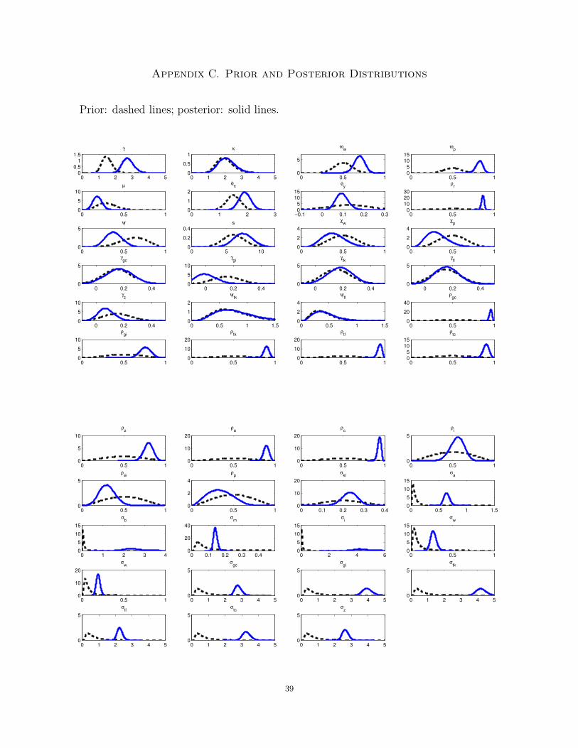
Appendix C. Prior and Posterior Distributions

Prior: dashed lines; posterior: solid lines.

0 1 2 3 4 50

0.51

1.5

γ

0 1 2 3 4 50

0.5

1

κ

0 0.5 10

5

ωw

0 0.5 105

1015

ωp

0 0.5 10

5

10

µ

0 1 2 30

1

2

φπ

−0.1 0 0.1 0.2 0.305

1015

φy

0 0.5 10

102030

ρr

0 0.5 10

5

ψ

0 5 100

0.2

0.4s

0 0.5 10

2

4

χw

0 0.5 10

2

4

χp

0 0.2 0.40

5

γgc

0 0.2 0.40

5

10

γgi

0 0.2 0.40

5

γtk

0 0.2 0.40

5

γtl

0 0.2 0.40

5

10

γz

0 0.5 1 1.50

1

2

ψtk

0 0.5 1 1.50

2

4

ψtl

0 0.5 10

20

40

ρgc

0 0.5 10

5

10

ρgi

0 0.5 10

10

20

ρtk

0 0.5 10

10

20

ρtl

0 0.5 105

1015

ρtc

0 0.5 10

5

10

ρz

0 0.5 10

10

20

ρa

0 0.5 10

10

20

ρc

0 0.5 10

5

ρi

0 0.5 10

5

ρw

0 0.5 10

2

4

ρp

0 0.1 0.2 0.3 0.40

10

20

σkl

0 0.5 1 1.50

5

10

15

σa

0 1 2 3 40

5

10

15

σb

0 0.1 0.2 0.3 0.40

20

40

σm

0 2 4 60

5

10

15

σi

0 0.5 10

5

10

15

σw

0 0.5 10

10

20

σw

0 1 2 3 4 50

5

σgc

0 1 2 3 4 50

5

σgi

0 1 2 3 4 50

5

σtk

0 1 2 3 4 50

5

σtl

0 1 2 3 4 50

5

σtc

0 1 2 3 4 50

5

σz

39

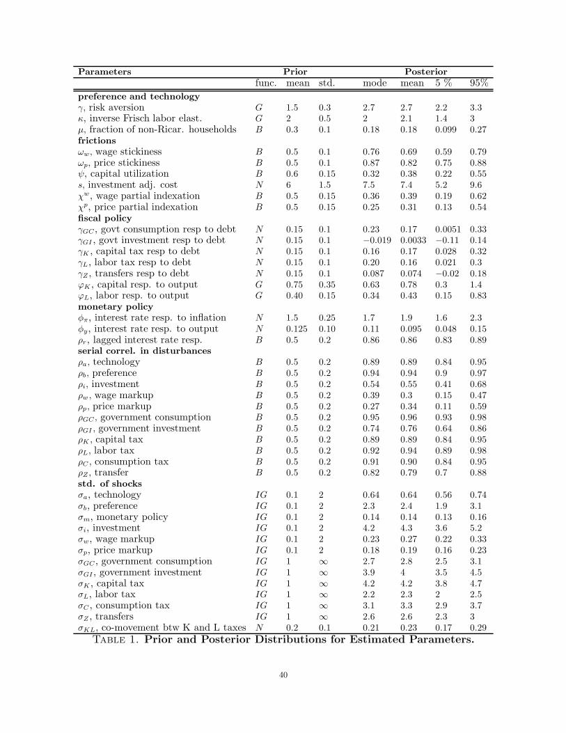
Parameters Prior Posterior

func. mean std. mode mean 5 % 95%

preference and technology

γ, risk aversion G 1.5 0.3 2.7 2.7 2.2 3.3κ, inverse Frisch labor elast. G 2 0.5 2 2.1 1.4 3µ, fraction of non-Ricar. households B 0.3 0.1 0.18 0.18 0.099 0.27frictions

ωw, wage stickiness B 0.5 0.1 0.76 0.69 0.59 0.79ωp, price stickiness B 0.5 0.1 0.87 0.82 0.75 0.88ψ, capital utilization B 0.6 0.15 0.32 0.38 0.22 0.55s, investment adj. cost N 6 1.5 7.5 7.4 5.2 9.6χw, wage partial indexation B 0.5 0.15 0.36 0.39 0.19 0.62χp, price partial indexation B 0.5 0.15 0.25 0.31 0.13 0.54fiscal policy

γGC , govt consumption resp to debt N 0.15 0.1 0.23 0.17 0.0051 0.33γGI , govt investment resp to debt N 0.15 0.1 −0.019 0.0033 −0.11 0.14γK , capital tax resp to debt N 0.15 0.1 0.16 0.17 0.028 0.32γL, labor tax resp to debt N 0.15 0.1 0.20 0.16 0.021 0.3γZ , transfers resp to debt N 0.15 0.1 0.087 0.074 −0.02 0.18ϕK , capital resp. to output G 0.75 0.35 0.63 0.78 0.3 1.4ϕL, labor resp. to output G 0.40 0.15 0.34 0.43 0.15 0.83monetary policy

φπ, interest rate resp. to inflation N 1.5 0.25 1.7 1.9 1.6 2.3φy, interest rate resp. to output N 0.125 0.10 0.11 0.095 0.048 0.15ρr, lagged interest rate resp. B 0.5 0.2 0.86 0.86 0.83 0.89serial correl. in disturbances

ρa, technology B 0.5 0.2 0.89 0.89 0.84 0.95ρb, preference B 0.5 0.2 0.94 0.94 0.9 0.97ρi, investment B 0.5 0.2 0.54 0.55 0.41 0.68ρw , wage markup B 0.5 0.2 0.39 0.3 0.15 0.47ρp, price markup B 0.5 0.2 0.27 0.34 0.11 0.59ρGC , government consumption B 0.5 0.2 0.95 0.96 0.93 0.98ρGI , government investment B 0.5 0.2 0.74 0.76 0.64 0.86ρK , capital tax B 0.5 0.2 0.89 0.89 0.84 0.95ρL, labor tax B 0.5 0.2 0.92 0.94 0.89 0.98ρC , consumption tax B 0.5 0.2 0.91 0.90 0.84 0.95ρZ , transfer B 0.5 0.2 0.82 0.79 0.7 0.88std. of shocks

σa, technology IG 0.1 2 0.64 0.64 0.56 0.74σb, preference IG 0.1 2 2.3 2.4 1.9 3.1σm, monetary policy IG 0.1 2 0.14 0.14 0.13 0.16σi, investment IG 0.1 2 4.2 4.3 3.6 5.2σw, wage markup IG 0.1 2 0.23 0.27 0.22 0.33σp, price markup IG 0.1 2 0.18 0.19 0.16 0.23σGC , government consumption IG 1 ∞ 2.7 2.8 2.5 3.1σGI , government investment IG 1 ∞ 3.9 4 3.5 4.5σK , capital tax IG 1 ∞ 4.2 4.2 3.8 4.7σL, labor tax IG 1 ∞ 2.2 2.3 2 2.5σC , consumption tax IG 1 ∞ 3.1 3.3 2.9 3.7σZ , transfers IG 1 ∞ 2.6 2.6 2.3 3σKL, co-movement btw K and L taxes N 0.2 0.1 0.21 0.23 0.17 0.29

Table 1. Prior and Posterior Distributions for Estimated Parameters.

40

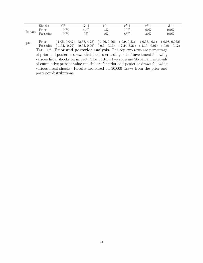
Shocks GC ↑ GI ↑ τK ↓ τL ↓ τC ↓ Z ↑

ImpactPrior 100% 44% 3% 70% 60% 100%Posterior 100% 0% 0% 83% 30% 100%

PVPrior (-1.05, 0.042) (2.38, 4.28) (-1.56, 0.66) (-0.9, 0.33) (-0.53, -0.1) (-0.98, 0.072)Posterior (-1.52, -0.29) (0.53, 0.99) (-0.6, -0.16) (-2.24, 3.21) (-1.15, -0.01) (-0.96, -0.12)

Table 2. Prior and posterior analysis. The top two rows are percentageof prior and posterior draws that lead to crowding out of investment followingvarious fiscal shocks on impact. The bottom two rows are 90-percent intervalsof cumulative present value multipliers for prior and posterior draws followingvarious fiscal shocks. Results are based on 30,000 draws from the prior andposterior distributions.

41

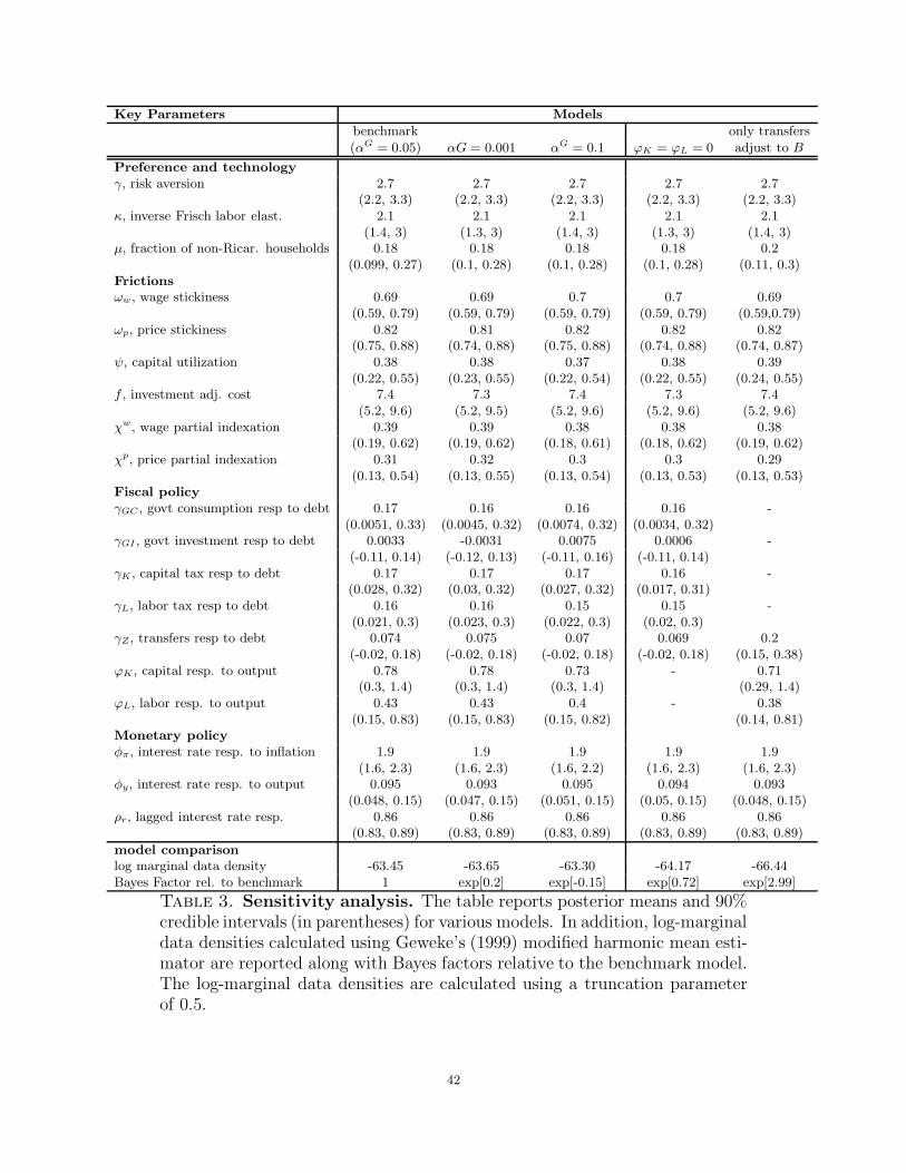
Key Parameters Models

benchmark only transfers

(αG = 0.05) αG = 0.001 αG = 0.1 ϕK = ϕL = 0 adjust to B

Preference and technology

γ, risk aversion 2.7 2.7 2.7 2.7 2.7(2.2, 3.3) (2.2, 3.3) (2.2, 3.3) (2.2, 3.3) (2.2, 3.3)

κ, inverse Frisch labor elast. 2.1 2.1 2.1 2.1 2.1(1.4, 3) (1.3, 3) (1.4, 3) (1.3, 3) (1.4, 3)

µ, fraction of non-Ricar. households 0.18 0.18 0.18 0.18 0.2(0.099, 0.27) (0.1, 0.28) (0.1, 0.28) (0.1, 0.28) (0.11, 0.3)

Frictions

ωw, wage stickiness 0.69 0.69 0.7 0.7 0.69(0.59, 0.79) (0.59, 0.79) (0.59, 0.79) (0.59, 0.79) (0.59,0.79)

ωp, price stickiness 0.82 0.81 0.82 0.82 0.82(0.75, 0.88) (0.74, 0.88) (0.75, 0.88) (0.74, 0.88) (0.74, 0.87)

ψ, capital utilization 0.38 0.38 0.37 0.38 0.39(0.22, 0.55) (0.23, 0.55) (0.22, 0.54) (0.22, 0.55) (0.24, 0.55)

f , investment adj. cost 7.4 7.3 7.4 7.3 7.4(5.2, 9.6) (5.2, 9.5) (5.2, 9.6) (5.2, 9.6) (5.2, 9.6)

χw, wage partial indexation 0.39 0.39 0.38 0.38 0.38(0.19, 0.62) (0.19, 0.62) (0.18, 0.61) (0.18, 0.62) (0.19, 0.62)

χp, price partial indexation 0.31 0.32 0.3 0.3 0.29(0.13, 0.54) (0.13, 0.55) (0.13, 0.54) (0.13, 0.53) (0.13, 0.53)

Fiscal policy

γGC, govt consumption resp to debt 0.17 0.16 0.16 0.16 -(0.0051, 0.33) (0.0045, 0.32) (0.0074, 0.32) (0.0034, 0.32)

γGI , govt investment resp to debt 0.0033 -0.0031 0.0075 0.0006 -(-0.11, 0.14) (-0.12, 0.13) (-0.11, 0.16) (-0.11, 0.14)

γK , capital tax resp to debt 0.17 0.17 0.17 0.16 -(0.028, 0.32) (0.03, 0.32) (0.027, 0.32) (0.017, 0.31)

γL, labor tax resp to debt 0.16 0.16 0.15 0.15 -(0.021, 0.3) (0.023, 0.3) (0.022, 0.3) (0.02, 0.3)

γZ, transfers resp to debt 0.074 0.075 0.07 0.069 0.2(-0.02, 0.18) (-0.02, 0.18) (-0.02, 0.18) (-0.02, 0.18) (0.15, 0.38)

ϕK , capital resp. to output 0.78 0.78 0.73 - 0.71(0.3, 1.4) (0.3, 1.4) (0.3, 1.4) (0.29, 1.4)

ϕL, labor resp. to output 0.43 0.43 0.4 - 0.38(0.15, 0.83) (0.15, 0.83) (0.15, 0.82) (0.14, 0.81)

Monetary policy

φπ, interest rate resp. to inflation 1.9 1.9 1.9 1.9 1.9(1.6, 2.3) (1.6, 2.3) (1.6, 2.2) (1.6, 2.3) (1.6, 2.3)

φy, interest rate resp. to output 0.095 0.093 0.095 0.094 0.093(0.048, 0.15) (0.047, 0.15) (0.051, 0.15) (0.05, 0.15) (0.048, 0.15)

ρr, lagged interest rate resp. 0.86 0.86 0.86 0.86 0.86(0.83, 0.89) (0.83, 0.89) (0.83, 0.89) (0.83, 0.89) (0.83, 0.89)

model comparison

log marginal data density -63.45 -63.65 -63.30 -64.17 -66.44Bayes Factor rel. to benchmark 1 exp[0.2] exp[-0.15] exp[0.72] exp[2.99]

Table 3. Sensitivity analysis. The table reports posterior means and 90%credible intervals (in parentheses) for various models. In addition, log-marginaldata densities calculated using Geweke’s (1999) modified harmonic mean esti-mator are reported along with Bayes factors relative to the benchmark model.The log-marginal data densities are calculated using a truncation parameterof 0.5.

42

Dependent variable All Shocks GC Shocks τLeShocksrt -0.0005 0.0008 0.0

(-0.015, 0.0117) (-0.0002, 0.0021) (-0.0003, 0.0002)r10t -0.0201 0.0182 -0.0058

(-0.2097, 0.1108) (-0.0043, 0.0406) (-0.0087, -0.0026)Table 4. Reduced-form regression results from simulated data series

using the mean posterior parameter estimates. Estimates are for β1

from the reduced-form regression xt = β0 + β1sbt + εt where the dependent

variable is either the one-period real interest rate rt or the ten-year real interestrate r10

t . The table reports the mean and 90% interval (in parenthesis) from500 simulated data series.

Dependent variablert r10

t

β1 0.0132 0.0269(0.0113, 0.0151) (-0.0045, 0.0614)

Table 5. Reduced-form regression results from the estimated se-

quence of the historical innovations. Estimates are for β1 from thereduced-form regression xt = β0 + β1s

bt + εt where the dependent variable

is either the one-period real interest rate rt or the ten-year real interest rater10t . The table reports the mean and 90% interval (in parentheses) from the

posterior distribution of parameter estimates.

Investment MultipliersBenchmark Varying αG No Output γ = 1,αG = 0.05 αG = 0.001 αG = 0.1 Responses κ = 1

GC ↑PV -0.69 -0.68 -0.68 -0.67 -0.52

impact -0.066 -0.066 -0.066 -0.064 -0.053

GI ↑PV 0.84 -0.34 6.58 3.48 2.6

impact -0.011 -0.029 0.084 0.032 0.024

τK ↓PV -0.42 -0.43 -0.42 -0.44 -0.45

impact -0.073 -0.074 -0.074 -0.077 -0.055

τL ↓PV 0.45 0.43 0.44 0.44 0.29

impact 0.0097 0.0096 0.0091 0.0091 0.007

τC ↓PV 0.33 0.32 0.33 0.33 0.42

impact -0.02 -0.02 -0.02 -0.02 0.015

Z ↑PV -0.42 -0.42 -0.42 -0.42 -0.32

impact -0.017 -0.017 -0.016 -0.017 -0.014Table 6. Robustness checks for the short and long run effects of

expansionary fiscal policy on investment. The rows display impact andcumulative present value (PV) multipliers for investment following variousshocks. PV multiplier calculations are described in footnote 12.

43

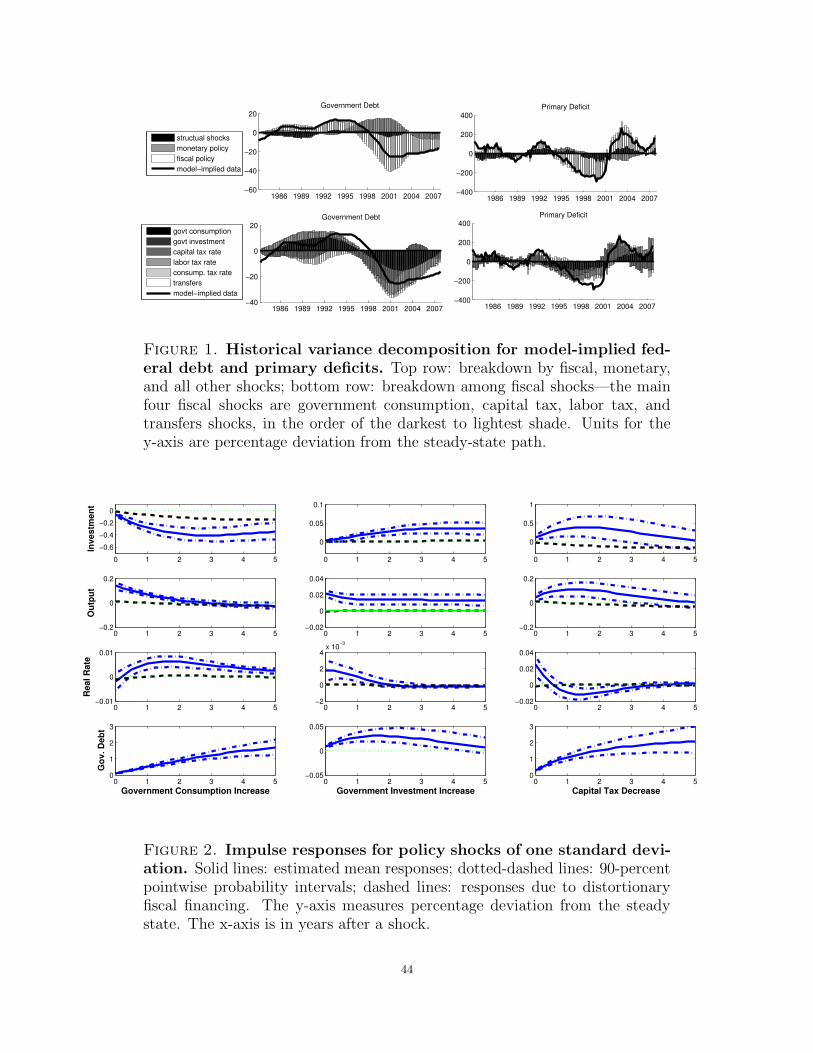
1986 1989 1992 1995 1998 2001 2004 2007−60

−40

−20

0

20Government Debt

structual shocks

monetary policy

fiscal policy

model−implied data

1986 1989 1992 1995 1998 2001 2004 2007−400

−200

0

200

400Primary Deficit

1986 1989 1992 1995 1998 2001 2004 2007−40

−20

0

20Government Debt

govt consumption

govt investment

capital tax rate

labor tax rate

consump. tax rate

transfers

model−implied data

1986 1989 1992 1995 1998 2001 2004 2007−400

−200

0

200

400Primary Deficit

Figure 1. Historical variance decomposition for model-implied fed-

eral debt and primary deficits. Top row: breakdown by fiscal, monetary,and all other shocks; bottom row: breakdown among fiscal shocks—the mainfour fiscal shocks are government consumption, capital tax, labor tax, andtransfers shocks, in the order of the darkest to lightest shade. Units for they-axis are percentage deviation from the steady-state path.

0 1 2 3 4 5

−0.6

−0.4

−0.2

0

Inv

es

tme

nt

0 1 2 3 4 5

0

0.05

0.1

0 1 2 3 4 5

0

0.5

1

0 1 2 3 4 5−0.2

0

0.2

Ou

tpu

t

0 1 2 3 4 5−0.02

0

0.02

0.04

0 1 2 3 4 5−0.2

0

0.2

0 1 2 3 4 5−0.01

0

0.01

Re

al

Ra

te

0 1 2 3 4 5−2

0

2

4x 10

−3

0 1 2 3 4 5−0.02

0

0.02

0.04

0 1 2 3 4 50

1

2

3

Government Consumption Increase

Go

v.

De

bt

0 1 2 3 4 5−0.05

0

0.05

Government Investment Increase0 1 2 3 4 5

0

1

2

3

Capital Tax Decrease

Figure 2. Impulse responses for policy shocks of one standard devi-

ation. Solid lines: estimated mean responses; dotted-dashed lines: 90-percentpointwise probability intervals; dashed lines: responses due to distortionaryfiscal financing. The y-axis measures percentage deviation from the steadystate. The x-axis is in years after a shock.

44

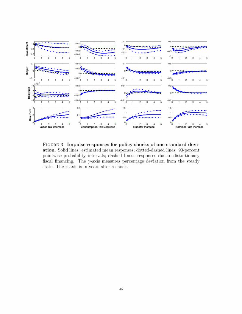
0 1 2 3 4 5

−0.4

−0.2

0

Inv

es

tme

nt

0 1 2 3 4 5

−0.04

−0.02

0

0.02

0 1 2 3 4 5

−0.2

−0.1

0

0.1

0 1 2 3 4 5−1

−0.5

0

0.5

0 1 2 3 4 5−0.1

0

0.1

Ou

tpu

t

0 1 2 3 4 5−0.02

0

0.02

0.04

0 1 2 3 4 5−0.1

0

0.1

0 1 2 3 4 5−0.5

0

0.5

0 1 2 3 4 5−5

0

5

10x 10

−3

Re

al

Ra

te

0 1 2 3 4 5−0.04

−0.02

0

0.02

0 1 2 3 4 5−0.01

0

0.01

0 1 2 3 4 5−0.2

0

0.2

0 1 2 3 4 50

2

4

Labor Tax Decrease

Go

v.

De

bt

0 1 2 3 4 50

0.1

0.2

Consumption Tax Decrease0 1 2 3 4 5

0

0.5

1

1.5

Transfer Increase0 1 2 3 4 5

0

0.5

1

1.5

Nominal Rate Increase

Figure 3. Impulse responses for policy shocks of one standard devi-

ation. Solid lines: estimated mean responses; dotted-dashed lines: 90-percentpointwise probability intervals; dashed lines: responses due to distortionaryfiscal financing. The y-axis measures percentage deviation from the steadystate. The x-axis is in years after a shock.

45

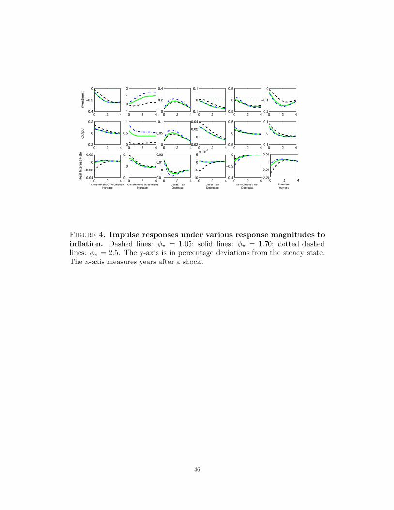
0 2 4−0.4

−0.2

0

Investm

ent

0 2 4−1

0

1

2

0 2 40

0.2

0.4

0 2 4−0.1

0

0.1

0 2 4−0.5

0

0.5

0 2 4−0.2

−0.1

0

0 2 4−0.2

0

0.2

Outp

ut

0 2 40

0.5

1

0 2 40

0.05

0.1

0 2 4−0.02

0

0.02

0.04

0 2 4−0.5

0

0.5

0 2 4−0.1

0

0.1

0 2 4−0.04

−0.02

0

0.02

Real In

tere

st R

ate

Government ConsumptionIncrease

0 2 4−0.1

0

0.1

Government InvestmentIncrease

0 2 4−0.01

0

0.01

0.02

Capital TaxDecrease

0 2 4−10

−5

0

5x 10

−3

Labor Tax Decrease

0 2 4−0.4

−0.2

0

Consumption Tax Decrease

0 2 4−0.02

−0.01

0

0.01

Transfers Increase

Figure 4. Impulse responses under various response magnitudes to

inflation. Dashed lines: φπ = 1.05; solid lines: φπ = 1.70; dotted dashedlines: φπ = 2.5. The y-axis is in percentage deviations from the steady state.The x-axis measures years after a shock.

46

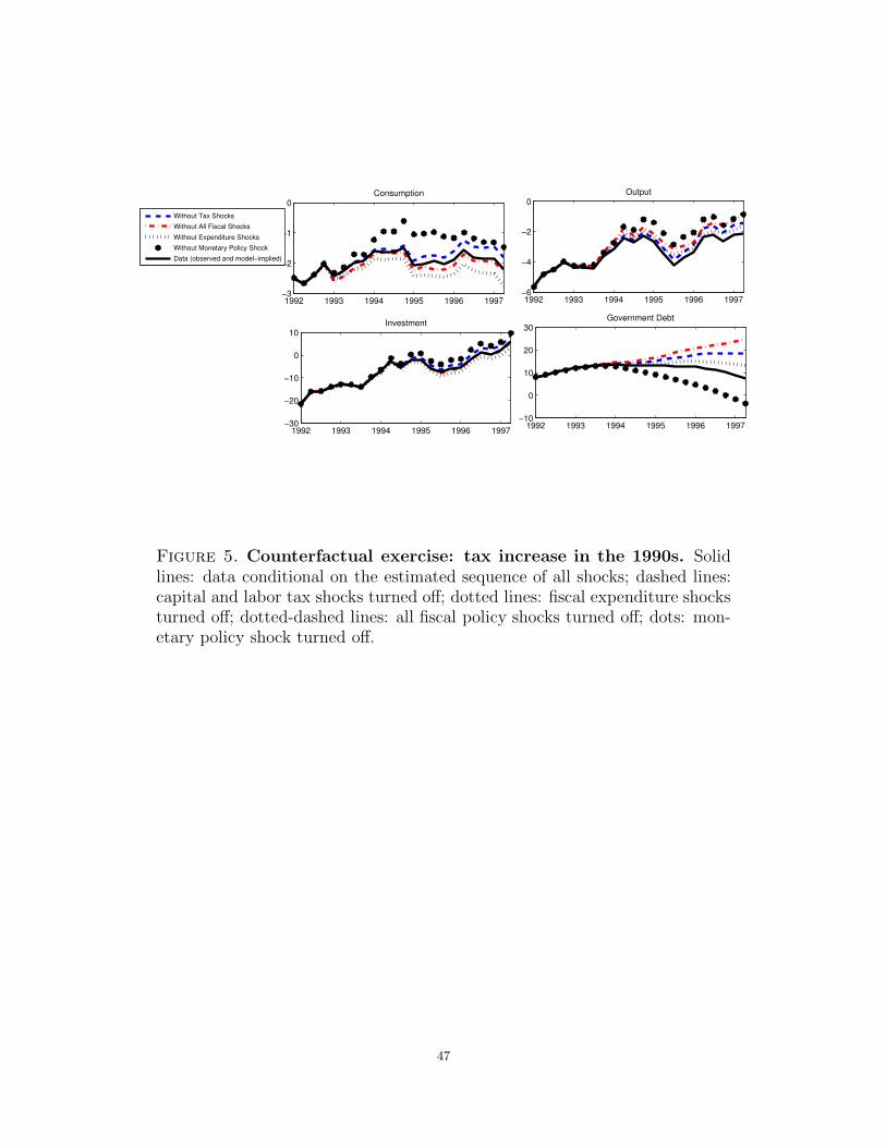
1992 1993 1994 1995 1996 1997−3

−2

−1

0Consumption

1992 1993 1994 1995 1996 1997−30

−20

−10

0

10Investment

1992 1993 1994 1995 1996 1997−6

−4

−2

0Output

Without Tax Shocks

Without All Fiscal Shocks

Without Expenditure Shocks

Without Monetary Policy Shock

Data (observed and model−implied)

1992 1993 1994 1995 1996 1997−10

0

10

20

30Government Debt

Figure 5. Counterfactual exercise: tax increase in the 1990s. Solidlines: data conditional on the estimated sequence of all shocks; dashed lines:capital and labor tax shocks turned off; dotted lines: fiscal expenditure shocksturned off; dotted-dashed lines: all fiscal policy shocks turned off; dots: mon-etary policy shock turned off.

47

2000 2001 20020

2

4Consumption

2000 2001 2002−5

0

5Output

2000 2001 2002−20

0

20Investment

2000 2001 2002−1

0

1Inflation

2000 2001 2002−1

0

1Nominal Interest Rate

2000 2001 2002−40

−20

0Government Debt

Without Tax Cuts

Without Monetary Shock

Data (observed or model implied)

Figure 6. Counterfactual exercise: tax cuts in 2001 and 2002. Solidlines: data conditional on the estimated sequence of all shocks; dashed lines:capital and labor tax shocks turned off; dotted-dashed lines: monetary policyshock turned off.

48

References

Alvarez-Lois, P., R. Harrison, L. Piscitelli, and A. Scott (2008): “On the ap-

plication and use of DSGE models,” Journal of Economic Dynamics and Control, 32(8),

2428–2452.

Barro, R. J. (1974): “Are Government Bonds Net Wealth?,” Journal of Political Economy,

82(6), 1095–1117.

Barth, J. R., G. Iden, and F. S. Russek (1984): “Do Federal Deficits Really Matter?,”

Contemporary Economic Policy, 3(1), 79–95.

Basu, S., and J. G. Fernald (1995): “Are Apparent Productive Spillovers a Figment of

Specification Error?,” Journal of Monetary Economics, 36(1), 165–188.

Baxter, M., and R. G. King (1993): “Fiscal Policy in General Equilibrium,” American

Economic Review, 83(3), 315–334.

Bernheim, B. D. (1989): “A Neoclassical Perspective on Budget Deficits,” Journal of

Economic Perspectives, 3(2), 55–72.

Bilbiie, F. O., A. Meier, and G. Mueller (forthcoming): “What Accounts for the

Change in U.S. Fiscal Policy Transmission?,” Journal of Money, Credit and Banking.

Blanchard, O. J. (1985): “Debts, Deficits, and Finite Horizons,” Journal of Political

Economy, 93(2), 223–247.

Bouakez, H., and N. Rebei (2007): “Why Does Private Consumption Rise After A

Government Spending Shock?,” Canadian Journal of Economics, 40(3), 954–979.

Browning, M., L. P. Hansen, and J. J. Heckman (1999): “Micro Data and General

Equilibrium Models,” in Handbook of Macroeconomics, ed. by J. B. Taylor and M. Wood-

ford, vol. 1A. Elsevier, Amsterdam.

Brunner, K., and A. H. Meltzer (1972): “Money, Debt, and Economic Activity,”

Journal of Political Economy, 80(5), 951–977.

Buiter, W. H., and J. Tobin (1980): “Fiscal and Monetary Policies, Capital For-

mation, and Economic Activity,” in The Government and Capital Formation, ed. by

49

G. Von Furstenberg, pp. 73–151. Ballinger Publishing Company, Cambridge, MA.

Calvo, G. A. (1983): “Staggered Prices in a Utility Maxmimizing Model,” Journal of

Monetary Economics, 12(3), 383–398.

Campbell, J. Y., and N. G. Mankiw (1989): “Consumption, Incomes, and Interest

Rates: Reinterpreting the Time Series Evidence,” in NBER Macroeconomics Annual 1989,

ed. by O. J. Blanchard, and S. Fischer, vol. 4, pp. 185–216. MIT Press, Cambridge, MA.

Canova, F. (2009): “Bridging Cyclical DSGE Models and the Raw Data,” Manuscript,

Centre de Recerca en Economia Internacional.

Chang, Y., T. Doh, and F. Schorfheide (2007): “Non-stationary Hours in a DSGE

Model,” Journal of Money, Credit and Banking, 39(6), 1357–1373.

Christiano, L. J., M. Eichenbaum, and C. L. Evans (2005): “Nominal Rigidities

and the Dynamic Effects of a Shock to Monetary Policy,” Journal of Political Economy,

113(1), 1–45.

Coenen, G., and R. Straub (2005): “Does Government Spending Crowd In Private

Consumption? Theory and Empirical Evidence for the Euro Area,” International Finance,

8(3), 437–470.

Colciago, A. (2007): “Rule of Thumb Consumers Meet Sticky Wages,” Munich Personal

RePEc Archive Working Paper No. 3756.

Congressional Budget Office (1984): “Deficits and Interest Rates: Empirical Find-

ings and Selected Bibliography,” in The Economic Outlook, February. Washington D.C.,

February.

(2009): The Long-Term Budget Outlook. Washington, D.C., June.

Davig, T., and E. M. Leeper (2006): Fluctuating Macro Policies and the Fiscal Theory,

NBER Macroeconomics Annual 2006. MIT Press, Cambridge.

(2009): “Monetary-Fiscal Policy Interactions and Fiscal Stimulus,” National Bu-

reau of Economic Research Working Paper No. 15133.

50

Del Negro, M., F. Schorfheide, F. Smets, and R. Wouters (2007): “On the Fit and

Forecasting Performance of New Keynesian Models,” Journal of Business and Economic

Statistics, 25(2), 123–162.

Dixit, A. K., and J. E. Stiglitz (1977): “Monopolistic Competition and Optimum

Product Diversity,” American Economic Review, 67(3), 297–308.

Domar, E. D. (1944): “The “Burden of the Debt” and the National Income,” American

Economic Review, 34(4), 798–827.

Elmendorf, D. W., and N. G. Mankiw (1999): “Government Debt,” in Handbook of

Macroeconomics, ed. by J. B. Taylor, and M. Woodford, vol. 1C, pp. 1615–1669. Elsevier

Science, Amsterdam.

Engen, E. M., and R. G. Hubbard (2005): “Federal Government Debt and Interest

Rates,” in NBER Macroeconomics Annual 2004, ed. by M. Gertler, and K. Rogoff. MIT

Press, Cambridge, MA.

Erceg, C. J., L. Guerrieri, and C. J. Gust (2005): “Expansionary Fiscal Shocks and

the Trade Deficit,” International Finance, 8(3), 363–397.

Evans, P., and G. Karras (1994): “Are Government Activities Productive? Evidence

from a Panel of U.S. States,” Review of Economic and Statistics, 76(1), 1–11.

Fernandez-Villaverde, J., P. Guerron-Quintana, and J. F. Rubio-Ramirez

(2010): “The New Macroeconometrics: A Bayesian Approach,” in The Oxford Hand-

book of Applied Bayesian Analysis, ed. by A. O’Hagan, and M. West. Oxford University

Press.

Fernandez-Villaverde, J., J. F. Rubio-Ramirez, T. J. Sargent, and M. W.

Watson (2007): “ABCs (and Ds) of Understanding VARs,” American Economic Review,

97(3), 1021–1026.

Forni, L., L. Monteforte, and L. Sessa (2009): “The General Equilibrium Effects

of Fiscal Policy: Estimates for the Euro Area,” Journal of Public Economics, 93(3-4),

559–585.

51

Freedman, C., M. Kumhof, D. Laxton, D. Muir, and S. Mursala (2009): “Fiscal

Stimulus to the Rescue? Short-Run Benefits and Potential Long-Run Costs of Fiscal

Deficits,” International Monetary Fund Working Paper No. 255.

Gale, W. G., and P. R. Orszag (2003): “The Economic Effects of Long-Term Fiscal

Discipline,” Urban-Brookings Tax Policy Center Discussion Paper No. 8.

(2004): Budget Deficits, National Saving, and Interest Rates, vol. 35(2004-2) of

Brookings Papers on Economic Activity. Brookings Institution Press.

Gali, J., J. D. Lopez-Salido, and J. Valles (2007): “Understanding the Effects of

Government Spending on Consumption,” Journal of the European Economic Association,

5(1), 227–270.

Geweke, J. (1999): “Using Simulation Methods for Bayesian Econometric Models: Infer-

ence, Development, and Communication,” Econometric Reviews, 18(1), 1–73.

(2005): Contemporary Bayesian Econometrics and Statistics. John Wiley and Sons,

Inc., Hoboken, NJ.

Greenwood, J., Z. Hercowitz, and P. Krusell (1997): “Long Run Implications of

Investment-Specific Technological Change,” American Economic Review, 87(3), 342–362.

(2000): “The Role of Investment-Specific Technological Change in the Business

Cycle,” European Economic Review, 44(1), 91–115.

Guvenen, F. (2006): “Reconciling Conflicting Evidence on the Elasticity of Intertemporal

Substitution: A Macroeconomic Perpsective,” Journal of Monetary Economics, 53(7),

1451–1472.

Iwata, Y. (2009): “Fiscal Policy in an Estimated DSGE Model of the Japanese Economy:

Do Non-Ricardian Households Explain All?,” Economic and Social Research Institute

Discussion Paper Series No. 219.

Jones, J. B. (2002): “Has Fiscal Policy Helped Stabilize the Postwar U.S. Economy?,”

Journal of Monetary Economics, 49(4), 709–746.

52

Kamps, C. (2004): The Dynamic Macroeconomic Effects of Public Capital. Springer, Berlin,

Germany.

Kim, J. (2000): “Constructing and Estimating a Realistic Optimizing Model of Monetary

Policy,” Journal of Monetary Economics, 45(2), 329–359.

Kohn, D. L. (1995): Inflation Indicators and Inflation Policy: Comment, NBER Macroe-

conomics Annual 1995. MIT Press, Cambridge, MA.

Kumhof, M., and D. Laxton (2007): “A Party Without a Hangover? On the Effects of

U.S. Government Deficits,” International Monetary Fund Working Paper 07/202.

Laubach, T. (2009): “New Evidence on the Interest Rate Effects of Budget Deficits and

Debt,” Journal of European Economic Association, 7(4), 858–885.

Leeper, E. M. (1991): “Equilibria Under ‘Active’ and ‘Passive’ Monetary and Fiscal Poli-

cies,” Journal of Monetary Economics, 27(1), 129–147.

Leeper, E. M., M. Plante, and N. Traum (2010): “Dynamics of Fiscal Financing in

the United States,” Journal of Econometrics, 156(2), 304–321.

Leeper, E. M., and C. A. Sims (1994): Toward a Modern Macroeconomic Model Usable

for Policy Analysis, NBER Macroeconomics Annual 1994. MIT Press, Cambridge, MA.

Leeper, E. M., and S.-C. S. Yang (2008): “Dynamic Scoring: Alternative Financing

Schemes,” Journal of Public Economics, 92(1-2), 159–182.

Leland, S. E. (1944): “Management of the Public Debt After the War,” American Eco-

nomic Review, 34(2, suppl.), 89–132.

Lerner, A. P. (1945): “Government Spending, Public Debt and Postwar Taxation,” In-

ternational Postwar Problems, 2(1), 13–34.

Lopez-Salido, J. D., and P. Rabanal (2006): “Government Spending and

Consumption-Hours Preferences,” “La Caixa” Working Paper Series No. 02/2006.

Ludvigson, S. (1996): “The Macroeconomic Effects of Government Debt in a Stochastic

Growth Model,” Journal of Monetary Economics, 38(1), 25–45.

53

Mankiw, N. G. (2000): “The Savers-Spenders Theory of Fiscal Policy,” American Eco-

nomic Review, 90(2), 120–125.

Modigliani, F. (1961): “Long-Run Implications of Alternative Fiscal Policies and the

Burden of the National Debt,” The Economic Journal, 71(284), 730–755.

Pereira, A. M., and R. F. de Frutos (1999): “Public Capital Accumulation and Private

Sector Performance,” Journal of Urban Economics, 46(2), 300–322.

Perotti, R. (2005): “Estimating the Effects of Fiscal Policy in OECD Countries,” Centre

for Economic Policy Research Discussion Paper 4842.

Ratto, M., W. Roeger, and J. in’t Veld (2009): “QUEST III: An Estimated Open-

Economy DSGE Model of the Euro Area with Fiscal and Monetary Policy,” Economic

Modeling, 26(1), 222–233.

Schmitt-Grohe, S., and M. Uribe (2004): “Optimal Operational Monetary Policy in

the Christiano-Eichenbaum-Evans Model of the U.S. Business Cycle,” National Bureau of

Economic Research Working Paper No. 10724.

(2008): “What’s ‘News’ in Business Cycles?,” National Bureau of Economic Re-

search Working Paper No. 14215.

Sims, C. A. (2001): “Solving Linear Rational Expectations Models,” Journal of Computa-

tional Economics, 20(1-2), 1–20.

Smets, F., and R. Wouters (2003): “An Estimated Dynamic Stochastic General Equi-

librium Model of the Euro Area,” Journal of the European Economic Association, 1(5),

1123–1175.

(2007): “Shocks and Frictions in U.S. Business Cycles: A Bayesian DSGE Ap-

proach,” American Economic Review, 97(3), 586–606.

Smetters, K. A. (1999): “Ricardian Equivalence: Long-Run Leviathan,” Journal of Public

Economics, 73(3), 395–421.

Taylor, J. B. (1993): “Discretion versus Policy Rules in Practice,” Carnegie-Rochester

Conference Series on Public Policy, 39(1), 195–214.

54

Tobin, J. (1969): “A General Equilibrium Approach to Monetary Theory,” Journal of

Money, Credit and Banking, 1(1), 15–29.

Uhlig, H. (2009): “Some Fiscal Calculus,” Paper prepared for the conference on “Monetary-

Fiscal Policy Interactions, Expectations, and Dynamics in the Current Economic Crisis”

at Princeton University.

Wallich, H. C. (1946): “Debt Management as an Instrument of Economic Policy,” Amer-

ican Economic Review, 36(3), 292–310.

Yang, S.-C. S. (2005): “Quantifying Tax Effects Under Policy Foresight,” Journal of

Monetary Economics, 52(8), 1557–1568.

Zubairy, S. (2009): “On Fiscal Multipliers: Estimates from a Medium Scale DSGE Model,”

Manuscript, Duke University.

55