1

Fiscal Multipliers for India

By

Sukanya Bose & N R Bhanumurthy*

Abstract: This paper attempts to present a framework for the estimation of fiscal multipliers for the Indian economy in the structural macroeconomic modelling tradition. Empirical estimates of short-run multipliers are obtained by giving shocks to a range of fiscal instruments - expenditures and taxes. As per our estimates, the values of capital expenditure multiplier, transfer payments multiplier and other revenue expenditure multiplier are 2.45, 0.98, and 0.99, respectively, while the tax multipliers are in the range of -1. Expenditure multipliers were also obtained in the presence of fiscal consolidation targets. These estimates again point to the strong multiplier effect of capital expenditure on output, and underscore the need to prioritize capital expenditure.

* The authors are Consultant and Professor, respectively, at the National Institute of Public Finance and Policy,

New Delhi. E-mail for correspondence: nrbmurthy@gmail.com

Acknowledgement: The earlier version of the paper is presented in a workshop at the Ministry of Finance,

Delhi. The authors would like to thank Raghuram G Rajan, KL Prasad, Arvinder Sachdeva, CKG Nair and

other workshop participants for their comments and suggestions. We have also benefitted greatly from the

discussions with Surajit Das, Kavita Rao and Mukesh Anand on specific aspects of the model. Overall guidance

from Sudipto Mundle in the initial phase of this work is gratefully acknowledged. However, the errors and

omissions are authors’ alone.

2

Fiscal Multipliers for India

I. Introduction

The concept of the multiplier was first formally introduced into economic theory by R.F. Kahn

(1931) and then was taken up by Keynes (1936). The textbook version of the Keynes-Kahn

multiplier says that if the government expenditure (G) goes up by one unit, it translates to more

than one unit increase in aggregate demand.1 The initial round of spending stimulates further

rounds of spending such that ultimately the effect on output is multiplier times the original

increase in spending. For an initial increase in government expenditure ∆G and marginal

propensity to consume (c), change in output ∆Y is k times ∆G, where k is the fiscal multiplier

and equals, k = 1/(1-c), under the assumption of closed economy. The value of fiscal multiplier

is the accumulated effect on output through various rounds of spending.2

Standard analysis of multiplier for an open economy tells us that if

Y=C{Y–t(Y)}+I+G+X – M(Y), then (Y/G)=[1/{(c(1-t)+m}]=multiplier

Where, „c‟ is marginal propensity to consume, „m‟ is marginal propensity to import and t is rate

of tax on income. Leakages on imports (besides savings and taxes) reduce the power of

government expenditure in an open economy.

In a situation where investment is determined by the growth of income itself, we have the

operation of what Lange (1943) had called the “compound multiplier” and Hicks (1950) had

called the “super multiplier”. Conceptually there is a difference between the multiplier and the

super multiplier that subsumes the effect of increased spending on investment via the

accelerator. However, when we talk about the empirical estimation of the aggregate effect of

changes in fiscal variables on the aggregate level of activity, we usually consider the combined

concept of super-multiplier as the fiscal multiplier.

Global financial crisis of 2008 and the consequent bailout of financial institutions and the

attempt by the states to revive economic activity through various fiscal stimulus measures have

caused a renewal of interest in this area. Naturally, while deciding on the nature and extent of

such stimulus, it has become important to measure the effectiveness of government spending

and tax-cuts on the aggregate level of activity and growth. Christina Romer, Chair of President

1 The textbook versions of the multiplier do not allude to the Keynes-Kalecki models, which interfaces

questions of growth with distribution.

2 [1/(1-c)] is the summation of the series c+c2+c3+… i.e. additions through multiple rounds.

3

Obama‟s Council of Economic Advisers, used multiplier values of about 1.5 in estimating the

job gains that would be generated by the $787 billion stimulus package approved by Congress

(Romer and Bernstein, 2009). Zandi (2008) presented detailed values of multipliers for each type

of government expenditure or tax cut, before the U.S. House Committee on Small Business. For

instance, Zandi‟s estimates showed that a $1 increase in food stamp payments boosts GDP by

$1.73 for the US economy.3 However, many others published smaller estimates of multipliers

(Barro, 2009; IMF, World Economic Outlook, 2010) that were later questioned when advanced

economies went into fiscal consolidation mode and the negative impact on economic activity

was far higher than what the small multipliers would suggest.4

While there is little consensus on the values of the multipliers in the literature, there are a

number of findings that are useful.

Most studies concur that the effects of government spending vary with the economic

environment. The size of spending multipliers in recessions and expansions vary

substantially with fiscal policy being considerably more effective in recessions than in

expansions. (Auerbach and Gorodnichenko, 2011)

A multiplier well in excess of one is possible when monetary policy is constrained by the

zero lower bound on nominal interest rate, and in this case welfare increases if

government purchases expand to partially fill the output gap that arises from the inability

to lower interest rates. (Michael Woodford, 2011; Christiano, Eichenbaum and Rebelo,

2009) Defence spending multipliers in the 1930s were as large as 2.5 on impact and 1.2

after the initial years (Almunia, Benetrix, Eichengreen, O‟Rourke and Rua, 2010). In

general, the multiplier is greater when interest rates do not respond to fiscal stimulus, and

there is virtually no crowding out.

In their paper, Ilzetzki, Mendoza and Végh (2011) tried to measure the real effects of

fiscal stimuli by showing that the impact of government expenditure shocks depends

crucially on key country characteristics, such as the level of development, exchange rate

regime, openness to trade, and public indebtedness. Based on a quarterly dataset of

government expenditure in 44 countries, by applying panel SVAR methodology, they

3 http://www.economy.com/mark-zandi/documents/Small%20Business_7_24_08.pdf

4 Blanchard and Leigh (2013) have regressed the forecast error for real GDP growth during 2010–11 on forecasts of fiscal consolidation for 2010–11 that were made in early 2010. The sample consists of 28 economies: the major advanced economies included in the G20 and the member countries of the EU for which forecasts were available Under rational expectations, and assuming that the correct forecast model has been used, the coefficient on planned fiscal consolidation should be zero. The authors find the coefficient on planned fiscal consolidation to be large, negative, and significant. Their analysis suggests that multipliers might be within the range 0.9 to 1.7. (also see World Economic Outlook, Sep, 2012, Box. 1.1)

4

have found that (i) the output effect of an increase in government consumption is larger

in industrial than in developing countries, (ii) the fiscal multiplier is relatively large in

economies operating under predetermined exchange rate but zero in economies

operating under flexible exchange rates; (iii) fiscal multipliers in open economies are

lower than in closed economies and (iv) fiscal multipliers in high-debt countries are zero.

The effectiveness of various government expenditures differs. Estimates of fiscal

multipliers for the Indian economy by Guimarães (2010) shows the government‟s current

expenditure multiplier as slightly above one on impact (one quarter), declining to around

0.5 after four to five quarters, suggesting partial crowding out of some private demand

component. The development spending (capital spending) multiplier is greater than 1,

suggesting that composition of spending matters, with a persistent effect even at 16

quarters. Tax revenue multiplier is about twice as large as current spending (same order

of magnitude of development spending), and remains significant after 8 quarters.

As part of reviving aggregate demand in the post-global crisis period, like many other countries,

India also undertook some fiscal stimulus measures. These measures were in the form of both

expenditures as well as taxes, which contributed to the deterioration of fiscal deficit by 4.2% of

GDP between 2007-8 and 2008-9. In our view, these stimulus measures were largely arbitrary.

Some of them were introduced even before the crisis set. There were hardly any analyses, ex

ante, to understand the impact of such measures in reviving demand. In other words, fiscal

policy measures are not based on the assessment on various fiscal multipliers. Hence, the output

response may not be as much as it was intended. In this study, an attempt has been made to fill

this gap, and to understand and estimate the size of various fiscal multipliers in India5.

There are various approaches to estimate the multiplier. The latest and popularly used approach

to calculate the multiplier is through structural vector autoregressive (SVAR) model (see

Blanchard and Perotti, 2002) by capturing the dynamic impacts (shocks) of changes in

government spending and taxes on output. Besides this approach to quantify the impact of a

fiscal policy shock, researchers have studied the impact of natural experiment of large military

build-ups (Barro, 1981). Another approach found in the literature has been to trace the effect on

GDP of increased public investment (Krishnamurty, 1985) and discretionary government

5 RBI, in its Annual Report 2011-12, (Box.II-16), presents some preliminary estimates for revenue and capital

outlay multipliers through a VAR framework. However, VAR model would not allow policy restrictions on the

fiscal deficit and other macroeconomic variables.

5

consumer expenditure (Bhattacharya, 1984) based on structural macroeconomic model6. In this

paper, we take the latter approach of estimating fiscal multipliers by building a fiscal block and

integrating with the existing NIPFP structural macroeconomic policy simulation model (Mundle

et.al. 2011).

The paper is organized as follows: after discussing the analytical framework for estimating the

multipliers for the Indian economy in Section II, in the next section we discuss the model

structure and model specification. Section IV and V present the results and policy conclusions,

respectively.

II. The Framework

The important fiscal policy levers in the hands of the Indian government are the budgetary

spending on the capital account and revenue account, and the various tax rates. It would be

worthwhile to see how changes in each of these policy levers impact the final output in the

economy. When there are inflationary pressures due to demand pull or when the overall growth

in the economy is faltering, estimates of fiscal multipliers would help make a conscious decision

on fiscal policy and help choose from among the various fiscal policy instruments. Or in

situations like the present one, where the economic growth is pallid at 6.2% in 2011-12 and at

5% for 2012-13 but any fiscal strategy has also to bear in mind the high levels of fiscal deficit,

estimates of multipliers become crucial.

In the following paragraphs we describe the fiscal policy instruments, their likely impact (fiscal

policy channels) and integrate it with a discussion on the official fiscal policy framework in India.

This would give a background to the theoretical model discussed in the following section. Our

focus would be the short-run.

1. Expenditure on the capital account by the government (center and states combined)

plays a crucial role in capital formation in the economy. An increase in capital

expenditure by the government translates to a much higher (more than proportionate

rise) public investment in the economy. Moreover, public investment crowds in private

investment resulting in even greater expenditure on the demand side and addition to

capital stock on the supply side.

6 Very recently, some studies have also used DSGE models.. However, as the DSGE models are based on micro foundations and require large datasets at the household level, which is not available for India, application of this approach could be difficult for India.

6

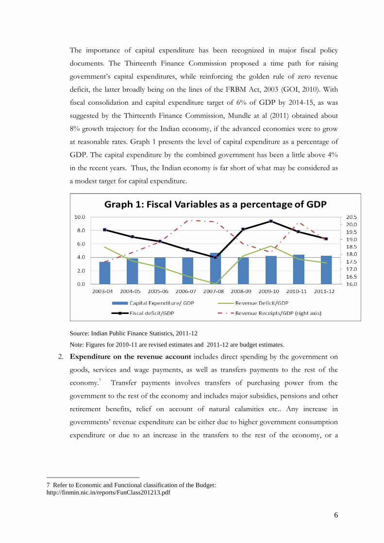
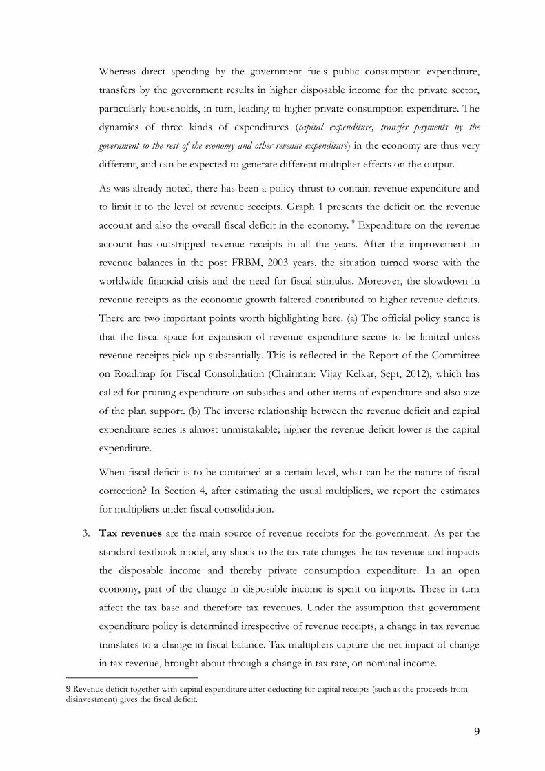
The importance of capital expenditure has been recognized in major fiscal policy

documents. The Thirteenth Finance Commission proposed a time path for raising

government‟s capital expenditures, while reinforcing the golden rule of zero revenue

deficit, the latter broadly being on the lines of the FRBM Act, 2003 (GOI, 2010). With

fiscal consolidation and capital expenditure target of 6% of GDP by 2014-15, as was

suggested by the Thirteenth Finance Commission, Mundle at al (2011) obtained about

8% growth trajectory for the Indian economy, if the advanced economies were to grow

at reasonable rates. Graph 1 presents the level of capital expenditure as a percentage of

GDP. The capital expenditure by the combined government has been a little above 4%

in the recent years. Thus, the Indian economy is far short of what may be considered as

a modest target for capital expenditure.

Source: Indian Public Finance Statistics, 2011-12

Note: Figures for 2010-11 are revised estimates and 2011-12 are budget estimates.

2. Expenditure on the revenue account includes direct spending by the government on

goods, services and wage payments, as well as transfers payments to the rest of the

economy.7 Transfer payments involves transfers of purchasing power from the

government to the rest of the economy and includes major subsidies, pensions and other

retirement benefits, relief on account of natural calamities etc.. Any increase in

governments‟ revenue expenditure can be either due to higher government consumption

expenditure or due to an increase in the transfers to the rest of the economy, or a

7 Refer to Economic and Functional classification of the Budget:

http://finmin.nic.in/reports/FunClass201213.pdf

7

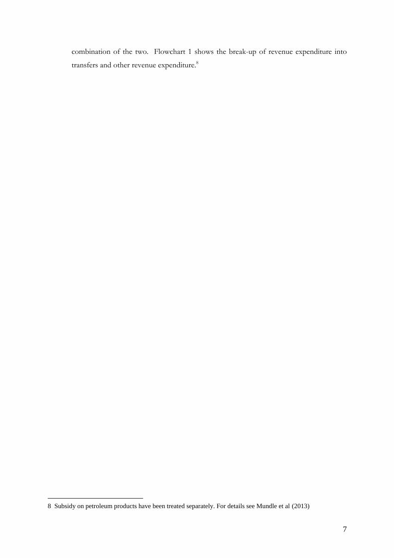
combination of the two. Flowchart 1 shows the break-up of revenue expenditure into

transfers and other revenue expenditure.8

8 Subsidy on petroleum products have been treated separately. For details see Mundle et al (2013)

8

FLOWCHART 1: FISCAL BLOCK

The exogenous and policy determined variables are denoted in upper case.

To obtain the multipliers, shocks are given to policy variables (indicated in italics bold underlined) and the impact traced through the system.

9

Whereas direct spending by the government fuels public consumption expenditure,

transfers by the government results in higher disposable income for the private sector,

particularly households, in turn, leading to higher private consumption expenditure. The

dynamics of three kinds of expenditures (capital expenditure, transfer payments by the

government to the rest of the economy and other revenue expenditure) in the economy are thus very

different, and can be expected to generate different multiplier effects on the output.

As was already noted, there has been a policy thrust to contain revenue expenditure and

to limit it to the level of revenue receipts. Graph 1 presents the deficit on the revenue

account and also the overall fiscal deficit in the economy. 9 Expenditure on the revenue

account has outstripped revenue receipts in all the years. After the improvement in

revenue balances in the post FRBM, 2003 years, the situation turned worse with the

worldwide financial crisis and the need for fiscal stimulus. Moreover, the slowdown in

revenue receipts as the economic growth faltered contributed to higher revenue deficits.

There are two important points worth highlighting here. (a) The official policy stance is

that the fiscal space for expansion of revenue expenditure seems to be limited unless

revenue receipts pick up substantially. This is reflected in the Report of the Committee

on Roadmap for Fiscal Consolidation (Chairman: Vijay Kelkar, Sept, 2012), which has

called for pruning expenditure on subsidies and other items of expenditure and also size

of the plan support. (b) The inverse relationship between the revenue deficit and capital

expenditure series is almost unmistakable; higher the revenue deficit lower is the capital

expenditure.

When fiscal deficit is to be contained at a certain level, what can be the nature of fiscal

correction? In Section 4, after estimating the usual multipliers, we report the estimates

for multipliers under fiscal consolidation.

3. Tax revenues are the main source of revenue receipts for the government. As per the

standard textbook model, any shock to the tax rate changes the tax revenue and impacts

the disposable income and thereby private consumption expenditure. In an open

economy, part of the change in disposable income is spent on imports. These in turn

affect the tax base and therefore tax revenues. Under the assumption that government

expenditure policy is determined irrespective of revenue receipts, a change in tax revenue

translates to a change in fiscal balance. Tax multipliers capture the net impact of change

in tax revenue, brought about through a change in tax rate, on nominal income.

9 Revenue deficit together with capital expenditure after deducting for capital receipts (such as the proceeds from disinvestment) gives the fiscal deficit.

10

Graph 1 gives the trends in revenue receipts in the recent period. Revenue receipts to

GDP ratio after rising steadily between 2003-4 to 2007-8, declined thereafter. One of the

reasons, though not the only one, was the tax concessions announced as part of fiscal

stimulus package.10 The tax structure in India consists of direct and indirect tax with the

indirect taxes dominating. Among the direct taxes, corporation tax and taxes on personal

income constitute more than 95% of the total direct tax collections of the combined

government. The indirect taxes, though more differentiated at present, are expected to

be consolidated under Goods and Services Tax (GST). The important taxes that are

going to be subsumed under GST are: general sales tax; union excise duties; Special

additional duty (SAD) and additional customs duty (ACD) component of customs duties

and service Tax. Indirect taxes on the petroleum sector are expected to remain outside

GST and customs revenues (excluding the countervailing duties) will continue to remain

separate.

Flow chart 1 divides the revenue receipts into indirect taxes on petroleum, net indirect

taxes (other than on petroleum), direct taxes, and all other revenue receipts. Alongside,

the determinants of the revenue flows are indicated. Tax revenues are a function of tax

base and tax rates. While corporation tax and income tax are taxes paid on income, GST

being a consumption-based tax, the tax base would be the consumption basket - private

and public consumption of goods and services. Expansion in tax base causes tax

revenues to increase, depending upon the tax buoyancy. Economic Survey, 2012-13

(GOI, 2013) reports a sharp fall in tax buoyancy in 2011- 12 which is reflected in the

decline in revenue receipts to GDP ratio in the latest year in Graph 1.

Normally, a higher tax rate causes an upward surge in tax collections. The opposite

however has also been observed. During the 1990s economic reforms in India,

rationalization of tax rates paid off in case of direct taxes, whereas in case of customs

duties, lower duties reduced the customs revenues. The elasticity of tax revenues to

change in tax rate is therefore of importance.

III. The Model

The NIPFP core model has been extended to address the question of fiscal multipliers. The

NIPFP model is a simultaneous equations system model developed for policy simulation.

10 There is no clear estimate for revenue loss from tax foregone, though the loss is expected to be significant

(see GOI, 2010, p.135).

11

Developed in the Tinbergen-Klein-Goldberger tradition of structural macroeconomic models, it

has been applied as a tool for policymakers to assess the likely consequences of alternative policy

choices. The model has been applied to track the macro-economic outcomes of a fiscal

consolidation path for the Thirteenth Finance Commission (Mundle et.al. 2011). It has also been

used to measure the immediate and medium term impact of an oil price policy shock and a

global oil price shock on macroeconomic outcomes such as growth, inflation and the fiscal

deficit. (Bhanumurthy et. al. 2012, Mundle et al. 2013). Further this has been used to address

some of the policy issues that are relevant for 12th Plan. The sub-components of the model can

easily be expanded if the policy question requires such detail on one or other aspect of the

model. The context and question specific structure can be added. The model is theoretically

eclectic rather than purist, picking up elements from different theoretical approaches as

supported by the empirical realities of the Indian economy.11

The core model has four blocks: macroeconomic block, fiscal block, external block and

monetary block each consisting of behavioural equations and identities. To estimate the fiscal

multipliers a satellite model was built where the fiscal block was disaggregated and expanded to

assess the impact of changes in various types of government expenditures and taxes on output.

The structure of the fiscal block was schematically presented in Flow chart 1. The model

specification of the fiscal block is presented below.

Fiscal Block: Model Specification

Nominal aggregate revenue expenditure of government (Et) is the sum of transfers to the private

sector by the government, TRt and the rest of the revenue expenditure of government in period

t, a policy variable,R

tE . Transfers to the private sector, TRt has two components: subsidy on oil

TRt O and transfers to other sectors of the economy, NO

tRT . We assume that the latter is policy

determined

R

ttt ETRE ˆ … … (1)

NO

t

O

tt RTTRTR ˆ … … (2)

11 For further discussion on the characteristics of the model see Mundle et al (2011).

12

TRtO is the subsidy to the oil companies, which is a function of domestic price of oil and

international price of POL basket.12

),ˆ( o

t

ao

t

O

t ppfTR

… … (3)

Where o

tp is international oil price of the Indian import POL basket and aO

tp is the administered

price of the oil basket. We assume that NO

tRT is policy determined.

R

tE determines the public consumption expenditure Gt whereas TRt flows into the private

disposable income and determines the private consumption expenditure Ct (not shown here).

)ˆ( R

tt EfG

… … (4)

Public investment is assumed to be a function of government capital expenditure:

… … (5)

where, is the capital expenditure of government in period t, a policy variable.

The level of government revenue (tax and non-tax) in period t is given by Tt and consists of

several components. These include personal income tax TtINC , and corporation tax, Tt

CORP (the

two main direct taxes), goods and services tax TtGST and customs duty Tt

CUS (the two main indirect

taxes), tax revenue from excise and custom duty from oil TtECO

,and sales tax revenue from oil,

TtSTO and all other tax and non-tax revenues, Tt

N .

… … (6)

Each tax is the function of the specific tax base and tax rates. Tax rates are policy handles, while

tax base is endogenously determined.

Personal income tax TtINC is assumed to be a function of income tax rate

INC

tt and non-

agricultural income, YtNA , while corporation tax Tt

CORP is assumed to be a function of corporate

tax rate CORP

tt and non-agricultural income, YtNA.

),ˆ( NA

t

INC

t

INC

t YtfT

… … (7)

12 Although the oil subsidy bill is expected to depend on the quantity of oil imports (sales), empirically it is found that oil subsidy is dependent largely on the price variables.

)ˆ( g

t

g

t SfI

g

tS

N

t

OST

t

OEC

t

CUST

t

GST

t

CORP

t

INC

tt TTTTTTTT

13

),ˆ( NA

t

CORP

t

CORP

t YtfT

… … (8)

The principal indirect tax being envisaged is the GST which would be a comprehensive tax for

goods and services.

),ˆ( tt

GST

t

GST

t GCtfT

… … (9)

Customs revenue collections (other than on oil which is accounted separately below) is a

function of net import demand and the policy determined average tariff rate, tU .

),ˆ( tt

CUST

t MUfT

… … (10)

Revenue from excise and custom duty from oil, TtEC-O

, levied as specific duty, is obtained by

applying the effective customs and excise tax rate to quantity of oil import, O

tQM .

O

t

OEC

t QMT ˆ … … (11)

Sales tax revenue from oil, TtST-O

, levied at an ad-valorem rate, is a function of administered

domestic price of oil, ao

tp and net oil import value (import minus export of oil), o

tNM .

),ˆ( o

t

ao

t

OST

t NMpfT … … (12)

Other revenue including the non-tax revenue and the residual taxes is assumed to be a function

of GDP.

)( t

N

t YfT … … … (13)

The fiscal deficit in period t, Ft, is given by

g

t

g

t

g

tt

g

ttt ODNTSEF ˆˆˆˆ … … … … (14)

Where g

tD is the aggregate market borrowing of the government in period t,g

tN is non-debt

capital receipts of the government (disinvestment etc.) and g

tO is the change in fiscal reserves.

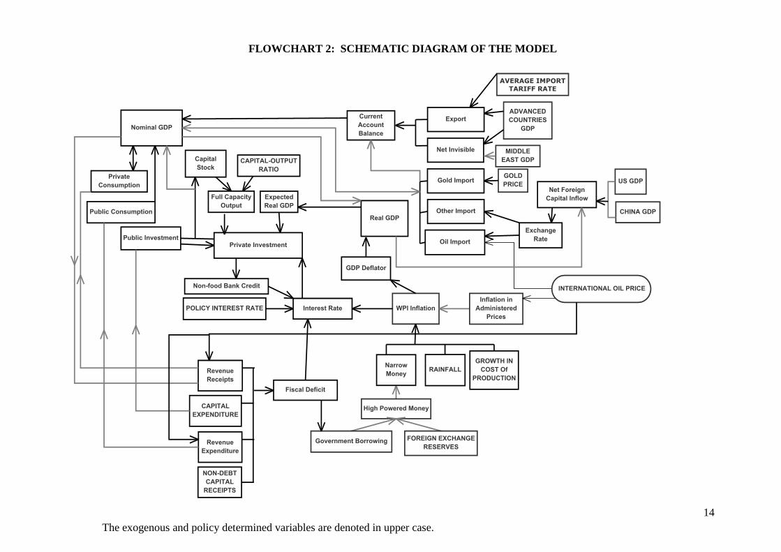
The above equations comprising of fiscal block are integrated into the larger core

macroeconomic model as shown is Flow Chart 2.

14

FLOWCHART 2: SCHEMATIC DIAGRAM OF THE MODEL

The exogenous and policy determined variables are denoted in upper case.

15

IV. Results

Annual data for the period 1991-2012 has been used for estimation of the model13. In this

exercise, we estimate fiscal multipliers under two scenarios: when there is no restriction on the

fiscal deficit and when there is a restriction on fiscal deficit as suggested by the Thirteenth

Finance Commission. To obtain the fiscal multipliers, a shock is given to the appropriate fiscal

policy variable in the year 2012-13 and its impact traced on output from the baseline. Table 1

presents the impact multipliers for expenditure changes, i.e., for one unit change in expenditure

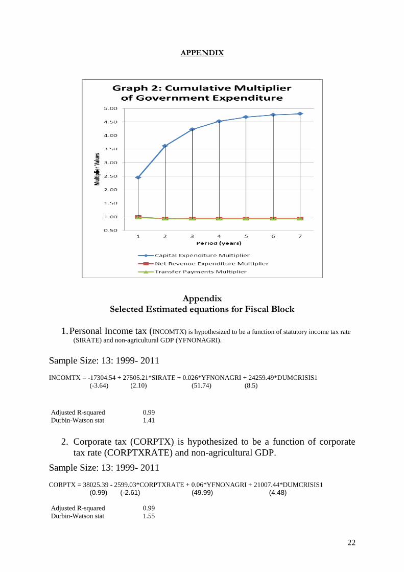
what is the change in output by the end of the year of the shock .(See Appendix for Graph 2 that

gives the cumulative expenditure multipliers over the subsequent years.)

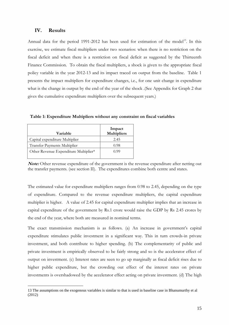
Table 1: Expenditure Multipliers without any constraint on fiscal variables

Variable Impact

Multipliers

Capital expenditure Multiplier 2.45

Transfer Payments Multiplier 0.98

Other Revenue Expenditure Multiplier* 0.99

Note: Other revenue expenditure of the government is the revenue expenditure after netting out the transfer payments. (see section II). The expenditures combine both centre and states.

The estimated value for expenditure multipliers ranges from 0.98 to 2.45, depending on the type

of expenditure. Compared to the revenue expenditure multipliers, the capital expenditure

multiplier is higher. A value of 2.45 for capital expenditure multiplier implies that an increase in

capital expenditure of the government by Rs.1 crore would raise the GDP by Rs 2.45 crores by

the end of the year, where both are measured in nominal terms.

The exact transmission mechanism is as follows. (a) An increase in government‟s capital

expenditure stimulates public investment in a significant way. This in turn crowds-in private

investment, and both contribute to higher spending. (b) The complementarity of public and

private investment is empirically observed to be fairly strong and so is the accelerator effect of

output on investment. (c) Interest rates are seen to go up marginally as fiscal deficit rises due to

higher public expenditure, but the crowding out effect of the interest rates on private

investments is overshadowed by the accelerator effect acting on private investment. (d) The high

13 The assumptions on the exogenous variables is similar to that is used in baseline case in Bhanumurthy et al

(2012)

16

import propensities (gold, oil and rest of the imports) results in substantial leakage from demand

and causes trade deficit to widen.14 The final multiplier values subsume, inter alia, these effects.

The revenue expenditure multipliers work through the consumption channels; whereas an

increase in transfer payments raises private consumption expenditure by raising the disposable

income of individuals, other revenue expenditure augments public consumption expenditure

directly. The multiplier effects of these expenditures is close to one and the crowding out of

private expenditure, as is popularly observed, is not seen either in the year of the shock or in the

subsequent years. (See Graph 2, Appendix.)

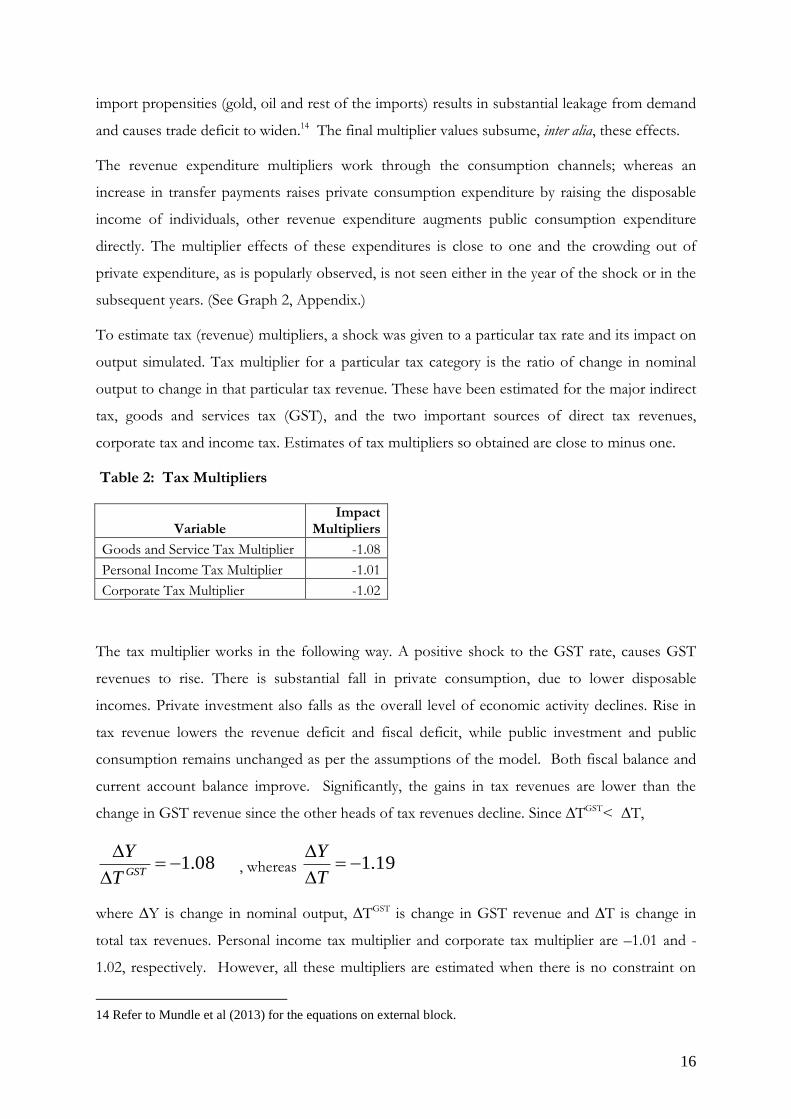
To estimate tax (revenue) multipliers, a shock was given to a particular tax rate and its impact on

output simulated. Tax multiplier for a particular tax category is the ratio of change in nominal

output to change in that particular tax revenue. These have been estimated for the major indirect

tax, goods and services tax (GST), and the two important sources of direct tax revenues,

corporate tax and income tax. Estimates of tax multipliers so obtained are close to minus one.

Table 2: Tax Multipliers

Variable Impact

Multipliers

Goods and Service Tax Multiplier -1.08

Personal Income Tax Multiplier -1.01

Corporate Tax Multiplier -1.02

The tax multiplier works in the following way. A positive shock to the GST rate, causes GST

revenues to rise. There is substantial fall in private consumption, due to lower disposable

incomes. Private investment also falls as the overall level of economic activity declines. Rise in

tax revenue lowers the revenue deficit and fiscal deficit, while public investment and public

consumption remains unchanged as per the assumptions of the model. Both fiscal balance and

current account balance improve. Significantly, the gains in tax revenues are lower than the

change in GST revenue since the other heads of tax revenues decline. Since ∆TGST< ∆T,

08.1

GSTT

Y , whereas 19.1

T

Y

where ∆Y is change in nominal output, ∆TGST is change in GST revenue and ∆T is change in

total tax revenues. Personal income tax multiplier and corporate tax multiplier are –1.01 and -

1.02, respectively. However, all these multipliers are estimated when there is no constraint on

14 Refer to Mundle et al (2013) for the equations on external block.

17

the fiscal (or revenue) deficit as suggested by Thirteenth Finance Commission (GOI, 2010) or by

the recent Kelkar committee (GOI, 2012). Next, we estimate the same multipliers after

endogenising the revised fiscal consolidation path suggested by the Kelkar committee.

Can there be negative fiscal multipliers?

Negative fiscal multipliers suggest that an economy is either experiencing conditions of contractionary fiscal expansions or expansionary fiscal contractions. The recent literature on this subject suggests that negative fiscal multipliers are feasible under some specific economic conditions. Especially since the recent Great recession, which lead to large fiscal stimulus measures across both developed and developing countries and subsequent uneven recovery, the interest on this subject has revived largely to determine the timing and the extent of fiscal austerity measures. A survey of recent studies (see Spilimbergo, et.al, 2009 for summary of the literature survey) on fiscal multipliers suggest that the size of multipliers is country-time-variant as it depends on the countries‟ domestic macroeconomic conditions, policies and also on the time series behaviour. This could depend on the quality of government expenditures as well. While relying on static multipliers is shown to be risky, sticking to the size derived from the pooled data is found to be equally irrelevant. The size of the multipliers based on the literature varies from positive, close to zero and, in some instances, negative. Following Keynesian framework, deriving positive fiscal multipliers is a norm and possibility of having negative multipliers is almost non-existent. However, if Ricardo‟s theory of balanced budgets holds or crowding-out impact is larger, then negative multiplier seems feasible. What determines the size-sign of the fiscal multiplier? Factors that affect the multiplier are: exchange rate regimes, extent of openness, size of the economy, level of public debt, expansion vs recession, health of financial sector, quality of government expenditure, health of public finances, monetary condition, etc. Based on the literature, negative fiscal multipliers are feasible during expansionary phase (Auerbach & Gorodnichenko, 2011); when a country has flexible exchange rate regime (Ilzetzki, et al, 2011; Corsetti, et al, 2012); if it is a developing country (Ilzetzki, et al, 2011); if the degree of openness is high (Ilzetzki, et al, 2011); if the debt-to-GDP ratio is very high (Ilzetzki, et al, 2011; Auerbach & Gorodnichenko, 2011; Nickel and Tudyka, 2013); if one has a fragile financial sector (Ilzetzki, et al, 2011; Corsetti, et al, 2012; de Cos and Moral-Benito, 2013), when the output gap is positive (Baum, et al, 2012, in the case of Canada and France), when the public finances are in bad shape (Corsetti, et al, 2012; de Cos and Moral-Benito, 2013), quality of expenditure (Alesina and Ardagna, 2009; Tervala, 2009), and depending on method of financing the deficits (Kandil, 2013). However, the findings of many of these studies have been widely discussed in the policy sphere and as well contested by researchers such that the debate remains inconclusive at the moment (see Mason & Jayadev, 2013, for this debate). At the moment, in India, many of the conditions that are discussed above appear to be existing and valid. However, one another crucial factor behind negative revenue expenditure multiplier in India in the context of fiscal consolidation constraint could be that there is a perfect substitution between revenue and capital expenditure. Thus, any positive shock to revenue expenditure tend to reduce capital expenditure to the extent of the shock as well as reduce private investments with the given fiscal deficit target and, hence, negative revenue expenditure multiplier. This is the basic philosophy of fiscal consolidation on which FRBM Act in India has been implemented. The result also indicates that if one has to strictly adhere to the FRBM, it is

18

also necessary to aim achieve sub-targets such target on revenue deficit as well as debt-to-GDP ratio. Sticking to fiscal deficit target alone may not be expansionary. Any relaxation on sub-targets may also followed by relaxation on fiscal deficit target under FRBM. A word of caution is that the fiscal multipliers estimated in current volatile (domestic as well as external) conditions, which could have affected the stability of macroeconomic parameters, needs to be used judiciously for present and future policy options (Blanchard and Leigh, 2013). However, there is a need for strong analytical frameworks for successful policy, which is the contribution of this study in the case of India.

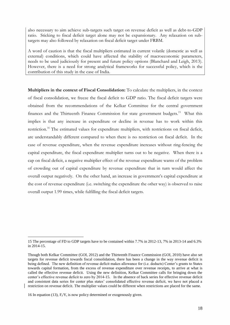
Multipliers in the context of Fiscal Consolidation: To calculate the multipliers, in the context

of fiscal consolidation, we freeze the fiscal deficit to GDP ratio. The fiscal deficit targets were

obtained from the recommendations of the Kelkar Committee for the central government

finances and the Thirteenth Finance Commission for state government budgets.15 What this

implies is that any increase in expenditure or decline in revenue has to work within this

restriction.16 The estimated values for expenditure multipliers, with restrictions on fiscal deficit,

are understandably different compared to when there is no restriction on fiscal deficit. In the

case of revenue expenditure, when the revenue expenditure increases without ring-fencing the

capital expenditure, the fiscal expenditure multiplier turns out to be negative. When there is a

cap on fiscal deficit, a negative multiplier effect of the revenue expenditure warns of the problem

of crowding out of capital expenditure by revenue expenditure that in turn would affect the

overall output negatively. On the other hand, an increase in government‟s capital expenditure at

the cost of revenue expenditure (i.e. switching the expenditure the other way) is observed to raise

overall output 1.99 times, while fulfilling the fiscal deficit targets.

15 The percentage of FD to GDP targets have to be contained within 7.7% in 2012-13, 7% in 2013-14 and 6.3%

in 2014-15.

Though both Kelkar Committee (GOI, 2012) and the Thirteenth Finance Commission (GOI, 2010) have also set

targets for revenue deficit towards fiscal consolidation, there has been a change in the way revenue deficit is

being defined. The new definition of revenue deficit makes allowance for (i.e. deducts) Center’s grants to States

towards capital formation, from the excess of revenue expenditure over revenue receipts, to arrive at what is

called the effective revenue deficit. Using the new definition, Kelkar Committee calls for bringing down the

center’s effective revenue deficit to zero by 2014-15. In the absence of back series for effective revenue deficit

and consistent data series for center plus states’ consolidated effective revenue deficit, we have not placed a

restriction on revenue deficit. The multiplier values could be different when restrictions are placed for the same.

16 In equation (13), Ft/Yt is now policy determined or exogenously given.

19

V. Policy Implications/ Conclusion

Despite policy targets that have sought to raise the capital expenditure by the government,

allocation for capital account expenditure continues to be a residual expenditure as observed in

recent budgetary exercises. The high value of the estimated capital expenditure multiplier points

to a high multiplier effect of capital expenditure on output, and underscores the need to

prioritize capital expenditure. As per our estimates, the values of capital expenditure multiplier,

transfer payments multiplier and other revenue expenditure multiplier are 2.45, 0.98, and 0.99,

respectively, while the tax multipliers are in the range of -1. This suggests that an increase in

output can be brought about by either an expenditure expansion or cut in tax rates, though with

different degrees of effectiveness. While an increase in output can be brought about through any

kind of public expenditure, the capital expenditure multiplier is the highest.

The present macroeconomic landscape in India demands a policy thrust that would combine

high growth in output while also bringing back fiscal discipline in the economy. Many

commentators have regarded the fiscal situation in the recent years as precarious and warned

about several adverse consequences stemming from it. However, to understand the

consequences of the type of government expenditures, there is a need to have an idea on the size

of fiscal multipliers, which for India unfortunately is not available at the moment in the literature.

The present study fills this gap and provides a framework as well as preliminary estimates of

various fiscal multipliers. The estimated size of multipliers suggest that the thrust of government

expenditure expansion has to shift in favour of capital expenditure.

20

References

Alesina F Alberto and Silivia Ardagna (2009), “Large Changes in Fiscal Policy: Taxes versus Spending”, NBER Working Paper Series, No.15348, October.

Almunia, Miguel, Agustin Benetrix, Barry Eichengreen, Kevin O‟Rourke and Gisela Rua (2010), “From Great Depression to Great Credit Crisis: Similarities, Differences and Lessons,” Economic Policy 25.

Auerbach, Alan J., and Yuriy Gorodnichenko (2011) “Fiscal Multipliers in Recession and Expansion,” NBER Working papers 17447.

Auerbach, A.J., and Y. Gorodnichenko, (2012), “Measuring the Output Responses to Fiscal

Policy,” American Economic Journal: Economic Policy, Vol. 4, pp. 1–27.

Barro, Robert J, 1981. "Output Effects of Government Purchases," Journal of Political Economy, University of Chicago Press, vol. 89(6), pages 1086-1121, December.

Barro, Robert, “Government spending is no free lunch,” Wall Street Journal (January 22, 2009).

Anja Baum, Marcos Poplawski-Ribeiro, and Anke Weber (2012) “Fiscal Multipliers and the State of the Economy”, IMF Working Paper WP/12/286.

Bhattacharya, B.B. (1984) Public Expenditure, Inflation and Growth: A Macro-Econometric Analysis for India, Oxford University Press, Delhi.

Blanchard, Oliver, and Roberto Perotti (2002) “An Empirical Characterization of the Dynamic Effects of Changes in Government Spending and Taxes on Output”, The Quarterly Journal of Economics, November

Blanchard, Oliver, and Daniel Leigh (2013) Growth Forecast Errors and Fiscal Multipliers, IMF Working Paper, January, 2013.

Bhanumurthy, N R, Surajit Das and Sukanya Bose (2012): “Oil price shock, pass-through policy and its impact on the Indian Economy, NIPFP Working Paper no.2012-99, March.

Christiano, Lawrence, and Martin Eichenbaum, and Sergio Rebelo (2009) “When is the Government Spending Multiplier is Large?”, NBER Working Paper 15394, October

Corsetti ,Giancarlo, Andre Meier, and Gernot J. Müller (2012) “What Determines Government

Spending Multipliers?”, IMF working Paper WP/12/150.

de Cos, Pablo Hernández and Enrique Moral-Benito (2013), “Fiscal Multipliers in Turbulent Times: The Case of Spain”, Banco de Espana Documentos de Trabajo No. 1309.

Guimarães Roberto (2010), “What Are The Effects of Fiscal Policy Shocks in India”, at http://macrofinance.nipfp.org.in/PDF/06_6Pr_Guimaraes_Fiscal%20Multipliers%20in%20India_2010_Conference.pdf as seen on 16/07/2012, March.

GOI (2010) Report of the Thirteenth Finance Commission, 2010-2015. (Chairman: Viijay Kelkar)

GOI (2012) Report of the Committee on Roadmap for Fiscal Consolidation (Chairman: Vijay Kelkar).

GOI (2013) Economic Survey, 2012-13, Ministry of Finance.

Ilzetzki, Ethan; Enrique G. Mendoza and Carlos A. Végh (2011), “How Big (Small?) are Fiscal Multipliers?”, IMF Working Paper, WP1152, March.

IMF (2010). World Economic Outlook, Recovery, Risk, and Rebalancing, October.

21

IMF (2012). World Economic Outlook, Coping with High Debt and Sluggish Growth, October.

Hicks, J. R. (1950), “A Contribution to the Theory of the Trade Cycle”, Clarendon Press, Oxford.

Kahn, R.F. (1931) “The Relation of Home Investment to Unemployment”, The Economic Journal, Vol. 41, No. 162, pp. 173-198, June.

Kandil, Magda Elsayed (2013) “Variation in the fiscal multiplier with the method of financing: evidence across industrial countries”, Applied Economics, Volume 45, Issue 35.

Keynes, J M. (1936) – “The General Theory of Employment, Interest and Money”, Book III, Chapter 10, Macmillan & Co. LTD, London.

Krishnamurty, K. (1985) “Inflation and growth: A model for India” in Krishnamurty, K. , & Pandit, V. Macroeconometric Modelling of The Indian Economy: Studies on Inflation and Growth. Delhi: Hindustan Publishing Corporation.

Lange, Oscar (1943), “The Theory of the Multiplier”, Econometrica, Vol. 11, No. 3/4, pp. 227-245, July – October.

Mason, J.W. and Arjun Jayadev (2013) “How the new Consensus in Macroeconomics Let Austerity Lose All the Intellectual Battles and Still Win the War,” Economic and Political Weekly, Vol. 48, No.2, p. 102- 111.

Mundle, Sudipto , N. R. Bhanumurthy and Surajit Das (2011), “Fiscal Consolidation with High Growth: A Policy Simulation Model for India” Economic Modelling 28 (2011) 2657–2668.

Mundle, Sudipto , N. R. Bhanumurthy and Sukanya Bose (2013), “Subsidy Elimination With and Without a Global Price Shock: The Macroeconomics of Oil Price Policy Reform”, forthcoming in a Festschrift for Dr Vijay Kelkar.

Nickel, Christiane and Andreas Tudyka (2013) “Fiscal Stimulus in times of High Debt: Reconsidering Multipliers and Twin Deficits”, European Central Bank Working Paper Series No.1513, February

Romer, Christina, and Jared Bernstein (2009) “The job impact of the American recovery and reinvestment plan,” http://otrans.3cdn.net/45593e8ecbd339d074_l3m6bt1te.pdf (accessed on 21st march, 2013.)

Spilimbergo, A., Symansky, S., and M. Schindler, 2009, “Fiscal Multipliers,” IMF Staff Position Note, SPN/09/11, May 2009.

Tervala Juha (2009), “The fiscal multiplier: positive or negative?” Aboa Centre for Economics

Discussion Paper No. 54, Turku.

Woodford, Michael (2011) “Simple Analytics of the Government Expenditure Multiplier”, American Economic Journal: Macroeconomics 3, pp. 1–35, January.

Zandi, Mark (2008) “A Second Quick Boost From Government Could Spark Recovery” http://www.economy.com/mark-zandi/documents/Small%20Business_7_24_08.pdf (accessed on April 1, 2013)

22

APPENDIX

Appendix

Selected Estimated equations for Fiscal Block

1. Personal Income tax (INCOMTX) is hypothesized to be a function of statutory income tax rate

(SIRATE) and non-agricultural GDP (YFNONAGRI).

Sample Size: 13: 1999- 2011

INCOMTX = -17304.54 + 27505.21*SIRATE + 0.026*YFNONAGRI + 24259.49*DUMCRISIS1

(-3.64) (2.10) (51.74) (8.5)

Adjusted R-squared 0.99

Durbin-Watson stat 1.41

2. Corporate tax (CORPTX) is hypothesized to be a function of corporate

tax rate (CORPTXRATE) and non-agricultural GDP.

Sample Size: 13: 1999- 2011

CORPTX = 38025.39 - 2599.03*CORPTXRATE + 0.06*YFNONAGRI + 21007.44*DUMCRISIS1

(0.99) (-2.61) (49.99) (4.48)

Adjusted R-squared 0.99

Durbin-Watson stat 1.55

23

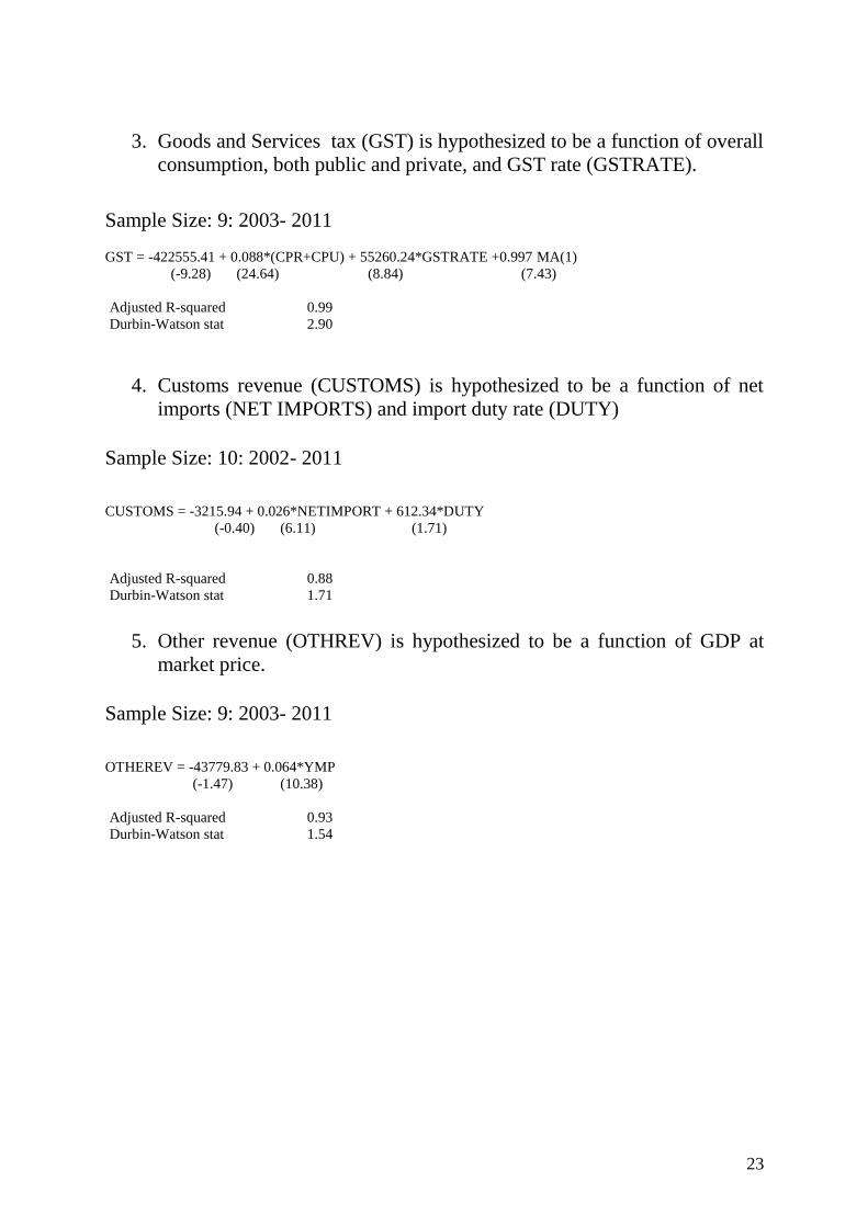
3. Goods and Services tax (GST) is hypothesized to be a function of overall

consumption, both public and private, and GST rate (GSTRATE).

Sample Size: 9: 2003- 2011

GST = -422555.41 + 0.088*(CPR+CPU) + 55260.24*GSTRATE +0.997 MA(1)

(-9.28) (24.64) (8.84) (7.43)

Adjusted R-squared 0.99

Durbin-Watson stat 2.90

4. Customs revenue (CUSTOMS) is hypothesized to be a function of net

imports (NET IMPORTS) and import duty rate (DUTY)

Sample Size: 10: 2002- 2011

CUSTOMS = -3215.94 + 0.026*NETIMPORT + 612.34*DUTY

(-0.40) (6.11) (1.71)

Adjusted R-squared

0.88

Durbin-Watson stat 1.71

5. Other revenue (OTHREV) is hypothesized to be a function of GDP at

market price.

Sample Size: 9: 2003- 2011

OTHEREV = -43779.83 + 0.064*YMP

(-1.47) (10.38)

Adjusted R-squared 0.93

Durbin-Watson stat 1.54