is “better data” better than “better data miners”? · is “better data” better than...

Is “Better Data” Better Than “Better Data Miners”?On the Benefits of Tuning SMOTE for Defect Prediction

Amritanshu AgrawalDepartment of Computer ScienceNorth Carolina State University

Raleigh, NC, [email protected]

Tim MenziesDepartment of Computer ScienceNorth Carolina State University

Raleigh, NC, [email protected]

ABSTRACTWe report and fix an important systematic error in prior studiesthat ranked classifiers for software analytics. Those studies did not(a) assess classifiers on multiple criteria and they did not (b) studyhow variations in the data affect the results. Hence, this paperapplies (a) multi-performance criteria while (b) fixing the weakerregions of the training data (using SMOTUNED, which is an auto-tuning version of SMOTE). This approach leads to dramaticallylarge increases in software defect predictions when applied in a5*5 cross-validation study for 3,681 JAVA classes (containing overa million lines of code) from open source systems, SMOTUNEDincreased AUC and recall by 60% and 20% respectively. These im-provements are independent of the classifier used to predict fordefects. Same kind of pattern (improvement) was observed when acomparative analysis of SMOTE and SMOTUNEDwas done againstthe most recent class imbalance technique.

In conclusion, for software analytic tasks like defect prediction,(1) data pre-processing can be more important than classifier choice,(2) ranking studies are incomplete without such pre-processing,and (3) SMOTUNED is a promising candidate for pre-processing.

KEYWORDSSearch based SE, defect prediction, classification, data analytics forsoftware engineering, SMOTE, imbalanced data, preprocessingACM Reference Format:Amritanshu Agrawal and Tim Menzies. 2018. Is “Better Data” Better Than“Better Data Miners”?: On the Benefits of Tuning SMOTE for Defect Pre-diction . In ICSE ’18: ICSE ’18: 40th International Conference on SoftwareEngineering , May 27-June 3, 2018, Gothenburg, Sweden. ACM, New York,NY, USA, 12 pages. https://doi.org/10.1145/3180155.3180197

1 INTRODUCTIONSoftware quality methods cost money and better quality costs expo-nentially more money [16, 66]. Given finite budgets, quality assur-ance resources are usually skewed towards areas known to be mostsafety critical or mission critical [34]. This leaves “blind spots”: re-gions of the system that may contain defects which may be missed.

Permission to make digital or hard copies of all or part of this work for personal orclassroom use is granted without fee provided that copies are not made or distributedfor profit or commercial advantage and that copies bear this notice and the full citationon the first page. Copyrights for components of this work owned by others than ACMmust be honored. Abstracting with credit is permitted. To copy otherwise, or republish,to post on servers or to redistribute to lists, requires prior specific permission and/or afee. Request permissions from [email protected] ’18, May 27-June 3, 2018, Gothenburg, Sweden© 2018 Association for Computing Machinery.ACM ISBN 978-1-4503-5638-1/18/05. . . $15.00https://doi.org/10.1145/3180155.3180197

Therefore, in addition to rigorously assessing critical areas, a paral-lel activity should be to sample the blind spots [37].

To sample those blind spots, many researchers use static codedefect predictors. Source code is divided into sections and researchersannotate the code with the number of issues known for each section.Classification algorithms are then applied to learn what static codeattributes distinguish between sections with few/many issues. Suchstatic code measures can be automatically extracted from the codebase with little effort even for very large software systems [44].

One perennial problem is what classifier should be used to buildpredictors? Many papers report ranking studies where a qualitymeasure is collected from classifiers when they are applied to datasets [13, 15–18, 21, 25–27, 29, 32, 33, 35, 40, 53, 62, 67]. These rankingstudies report which classifiers generate best predictors.

Research of this paper began with the question would the use ofdata pre-processor change the rankings of classifiers? SE data sets areoften imbalanced, i.e., the data in the target class is overwhelmed byan over-abundance of information about everything else except thetarget [36]. As shown in the literature review of this paper, in theoverwhelming majority of papers (85%), SE research uses SMOTEto fix data imbalance [7] but SMOTE is controlled by numerousparameters which usually are tuned using engineering expertiseor left at their default values. This paper proposes SMOTUNED,an automatic method for setting those parameters which whenassessed on defect data from 3,681 classes (over a million linesof code) taken from open source JAVA systems, SMOTUNED out-performed both the original SMOTE [7] as well as state-of-the-artmethod [4].

To assess, we ask four questions:

• RQ1: Are the default “off-the-shelf” parameters for SMOTE ap-propriate for all data sets?

Result 1SMOTUNED learned different parameters for each data set, all ofwhich were very different from default SMOTE.

• RQ2: Is there any benefit in tuning the default parameters ofSMOTE for each new data set?

Result 2Performance improvements using SMOTUNED are dramaticallylarge, e.g., improvements in AUC up to 60% against SMOTE.

In those results, we see that while no learner was best across alldata sets and performance criteria, SMOTUNED was most oftenseen in the best results. That is, creating better training data mightbe more important than the subsequent choice of classifiers.

arX

iv:1

705.

0369

7v3

[cs

.SE

] 2

0 Fe

b 20

18

https://doi.org/10.1145/3180155.3180197

https://doi.org/10.1145/3180155.3180197

ICSE ’18, May 27-June 3, 2018, Gothenburg, Sweden Amritanshu Agrawal and Tim Menzies

• RQ3: In terms of runtimes, is the cost of running SMOTUNEDworth the performance improvement?

Result 3SMOTUNED terminates in under two minutes, i.e., fast enough torecommend its widespread use.

• RQ4: How does SMOTUNED perform against the recent classimbalance technique?

Result 4SMOTUNED performs better than a very recent imbalance handlingtechnique proposed by Bennin et al. [4].

In summary, the contributions of this paper are:

• The discovery of an important systematic error in many priorranking studies, i.e., all of [13, 15–18, 21, 25–27, 29, 32, 33, 35,40, 53, 62, 67].

• A novel application of search-based SE (SMOTUNED) to handleclass imbalance that out-performs the prior state-of-the-art.

• Dramatically large improvements in defect predictors.• Potentially, for any other software analytics task that uses clas-sifiers, a way to improve those learners as well.

• A methodology for assessing the value of pre-processing datasets in software analytics.

• A reproduction package to reproduce our results then (perhaps)to improve or refute our results (Available to download fromhttp://tiny.cc/smotuned).

The rest of this paper is structured as follows: Section 2.1 gives anoverview on software defect prediction. Section 2.2 talks about allthe performance criteria used in this paper. Section 2.3 explainsthe problem of class imbalance in defect prediction. Assessmentof the previous ranking studies is done in Section 2.4. Section 2.5introduces SMOTE and discusses how SMOTE has been used in lit-erature. Section 2.6 provides the definition of SMOTUNED. Section3 describes the experimental setup of this paper and above researchquestions are answered in Section 4. Lastly, we discuss the validityof our results and a section describing our conclusions.

Note that the experiments of this paper only make conclusionsabout software analytics for defect prediction. That said, many othersoftware analytics tasks use the same classifiers explored here: fornon-parametric sensitivity analysis [41], as a pre-processor to buildthe tree used to infer quality improvement plans [31], to predictGithub issue close time [55], and many more. That is, potentially,SMOTUNED is a sub-routine that could improve many softwareanalytics tasks. This could be a highly fruitful direction for futureresearch.

2 BACKGROUND AND MOTIVATION2.1 Defect PredictionSoftware programmers are intelligent, but busy people. Such busypeople often introduce defects into the code they write [20]. Testingsoftware for defects is expensive and most software assessmentbudgets are finite. Meanwhile, assessment effectiveness increasesexponentially with assessment effort [16]. Such exponential costsexhaust finite resources so software developers must carefully de-cide what parts of their code need most testing.

A variety of approaches have been proposed to recognize defect-prone software components using code metrics (lines of code, com-plexity) [10, 38, 40, 45, 58] or process metrics (number of changes,recent activity) [22]. Other work, such as that of Bird et al. [5],indicated that it is possible to predict which components (for e.g.,modules) are likely locations of defect occurrence using a compo-nent’s development history and dependency structure. Predictionmodels based on the topological properties of components withinthem have also proven to be accurate [71].

The lesson of all the above is that the probable location of futuredefects can be guessed using logs of past defects [6, 21]. These logsmight summarize software components using static code metricssuch as McCabes cyclomatic complexity, Briands coupling metrics,dependencies between binaries, or the CK metrics [8] (which isdescribed in Table 1). One advantage with CK metrics is that theyare simple to compute and hence, they are widely used. Radjenovićet al. [53] reported that in the static code defect prediction, the CKmetrics are used twice as much (49%) as more traditional sourcecode metrics such as McCabes (27%) or process metrics (24%). Thestatic code measures that can be extracted from a software is shownin Table 1. Note that such attributes can be automatically collected,even for very large systems [44]. Other methods, like manual codereviews, are far slower and far more labor intensive.

Static code defect predictors are remarkably fast and effective.Given the current generation of data mining tools, it can be a matterof just a few seconds to learn a defect predictor (see the runtimesin Table 9 of reference [16]). Further, in a recent study by Rahmanet al. [54], found no significant differences in the cost-effectivenessof (a) static code analysis tools FindBugs and Jlint, and (b) staticcode defect predictors. This is an interesting result since it is muchslower to adapt static code analyzers to new languages than defectpredictors (since the latter just requires hacking together some newstatic code metrics extractors).

2.2 Performance CriteriaFormally, defect prediction is a binary classification problem. Theperformance of a defect predictor can be assessed via a confusionmatrix like Table 2 where a “positive” output is the defective classunder study and a “negative” output is the non-defective one.

Table 2: Results MatrixActual

Prediction false truedefect-free TN FNdefective FP TP

Further, “false” means thelearner got it wrong and“true” means the learner cor-rectly identified a fault or non-fault module. Hence, Table 2has four quadrants containing,e.g., FP which denotes “false positive”.

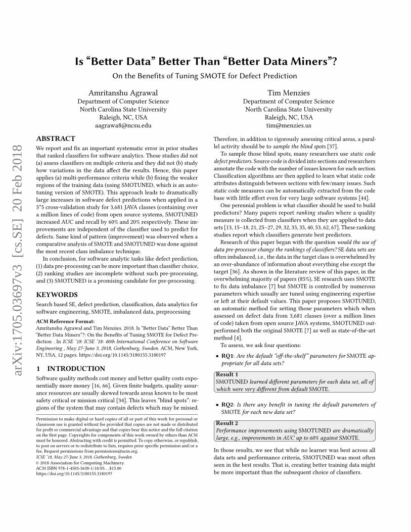
From this matrix, we can define performance measures like:• Recall = pd = TP/(TP + FN )• Precision = prec = TP/(TP + FP)• False Alarm = p f = FP/(FP + TN )• Area Under Curve (AUC), which is the area covered by anROC curve [11, 60] in which the X-axis represents, false positiverate and the Y-axis represents true positive rate.As shown in Figure 1, a typical predictor must “trade-off” be-

tween false alarm and recall. This is because the more sensitive thedetector, the more often it triggers and the higher its recall. If a

http://tiny.cc/smotuned

Is “Better Data” Better Than “Better Data Miners”? ICSE ’18, May 27-June 3, 2018, Gothenburg, Sweden

Table 1: OO CK code metrics used for all studies in this paper. The last line shown, denotes the dependent variable.

amc average method complexity e.g., number of JAVA byte codesavg, cc average McCabe average McCabe’s cyclomatic complexity seen in classca afferent couplings how many other classes use the specific class.cam cohesion amongst classes summation of number of different types of method parameters in every method divided by a multiplication of

number of different method parameter types in whole class and number of methods.cbm coupling between methods total number of new/redefined methods to which all the inherited methods are coupledcbo coupling between objects increased when the methods of one class access services of another.ce efferent couplings how many other classes is used by the specific class.dam data access ratio of the number of private (protected) attributes to the total number of attributesdit depth of inheritance treeic inheritance coupling number of parent classes to which a given class is coupled

lcom lack of cohesion in methods number of pairs of methods that do not share a reference to an case variable.locm3 another lack of cohesion measure ifm, a are the number ofmethods, attr ibutes in a class number and µ(a) is the number of methods accessing

an attribute, then lcom3 = (( 1a∑, ja µ(a, j)) −m)/(1 −m).

loc lines of codemax, cc maximum McCabe maximum McCabe’s cyclomatic complexity seen in classmfa functional abstraction no. of methods inherited by a class plus no. of methods accessible by member methods of the classmoa aggregation count of the number of data declarations (class fields) whose types are user defined classesnoc number of childrennpm number of public methodsrfc response for a class number of methods invoked in response to a message to the object.wmc weighted methods per class

nDefects raw defect counts numeric: number of defects found in post-release bug-tracking systems.defects present? boolean if nDefects > 0 then true else false

detector triggers more often, it also raises more false alarms. Hence,when increasing recall, we should expect the false alarm rate toincrease (ideally, not by very much).

Figure 1: Trade-offs false alarm vsrecall (probability of detection).

There are manymore ways to eval-uate defect predic-tors besides the fourlisted above. Previ-ously, Menzies et al.catalogued dozensof them (see Table23.2 of [39]) andeven several novelones were proposed(balance, G-measure [38]).But no evaluation criteria is “best” since different criteria are appro-priate in different business contexts. For e.g., as shown in Figure 1,when dealing with safety-critical applications, management may be“risk adverse” and hence many elect to maximize recall, regardlessof the time wasted exploring false alarm. Similarly, when rushingsome non-safety critical application to market, management maybe “cost adverse” and elect tominimize false alarm since this avoidsdistractions to the developers.

In summary, there are numerous evaluation criteria and numer-ous business contexts where different criteria might be preferredby different local business users. In response to the cornucopia ofevaluation criteria, we make the following recommendations: a)do evaluate learners on more than one criteria, b) do not evaluatelearners on all criteria (there are too many), and instead, apply thecriteria widely seen in the literature. Applying this advice, this pa-per evaluates the defect predictors using the four criteria mentionedabove (since these are widely reported in the literature [16, 17]))but not other criteria that have yet to gain a wide acceptance (i.e.,balance and G-measure).

2.3 Defect Prediction and Class ImbalanceClass imbalance is concerned with the situation in where someclasses of data are highly under-represented compared to other

classes [23]. By convention, the under-represented class is calledthe minority class, and correspondingly the class which is over-represented is called the majority class. In this paper, we say thatclass imbalance isworsewhen the ratio of minority class to majorityincreases, that is, class-imbalance of 5:95 is worse than 20:80. Menzieset al. [36] reported SE data sets often contain class imbalance. Intheir examples, they showed static code defect prediction data setswith class imbalances of 1:7; 1:9; 1:10; 1:13; 1:16; 1:249.

The problem of class imbalance is sometimes discussed in thesoftware analytics community. Hall et al. [21] found that modelsbased on C4.5 under-perform if they have imbalanced data whileNaive Bayes and Logistic regression perform relatively better. Theirgeneral recommendation is to not use imbalanced data. Some re-searchers offer preliminary explorations into methods that mightmitigate for class imbalance. Wang et al. [67] and Yu et al. [69]validated the Hall et al. results and concluded that the performanceof C4.5 is unstable on imbalanced data sets while Random Forestand Naive Bayes are more stable. Yan et al. [68] performed fuzzylogic and rules to overcome the imbalance problem, but they onlyexplored one kind of learner (Support Vector Machines). Pelayo etal. [49] studied the effects of the percentage of oversampling andundersampling done. They found out that different percentage ofeach helps improve the accuracies of decision tree learner for defectprediction using CK metrics. Menzies et al. [42] undersampled thenon-defect class to balance training data and reported how little in-formation was required to learn a defect predictor. They found thatthrowing away data does not degrade the performance of NaiveBayes and C4.5 decision trees. Other papers [49, 50, 57] have shownthe usefulness of resampling based on different learners.

We note that many researchers in this area [19, 67, 69] refer tothe SMOTE method explored in this paper, but only in the contextof future work. One rare exception to this general pattern is therecent paper by Bennin et al. [4], which we explored as part of RQ4.

2.4 Ranking StudiesA constant problem in defect prediction is what classifier shouldbe applied to build the defect predictors? To address this problem,many researchers run ranking studies where performance scores


Table 3: Classifiers used in this study. Rankings from Ghotra et al. [17].

RANK LEARNER NOTES1 “best” RF= random forest Random forest of entropy-based decision trees.

LR=Logistic regression A generalized linear regression model.2 KNN= K-means Classify a new instance by finding “k” examples of similar instances. Ghortra et al. suggested K = 8.

NB= Naive Bayes Classify a new instance by (a) collecting mean and standard deviations of attributes in old instances of differentclasses; (b) return the class whose attributes are statistically most similar to the new instance.

3 DT= decision trees Recursively divide data by selecting attribute splits that reduce the entropy of the class distribution.4 “worst” SVM= support vector machines Map the raw data into a higher-dimensional space where it is easier to distinguish the examples.

Table 4: 22 highly cited Software Defect prediction studies.

Ref Year Citations RankedClassifiers?

Evaluatedusing

multiplecriteria?

ConsideredData

Imbalance?

[38] 2007 855 ✓ 2 ✗[32] 2008 607 ✓ 1 ✗[13] 2008 298 ✓ 2 ✗[40] 2010 178 ✓ 3 ✗[18] 2008 159 ✓ 1 ✗[30] 2011 153 ✓ 2 ✗[53] 2013 150 ✓ 1 ✗[25] 2008 133 ✓ 1 ✗[67] 2013 115 ✓ 1 ✓[35] 2009 92 ✓ 1 ✗[33] 2012 79 ✓ 2 ✗[28] 2007 73 ✗ 2 ✓[49] 2007 66 ✗ 1 ✓[27] 2009 62 ✓ 3 ✗[29] 2010 60 ✓ 1 ✓[17] 2015 53 ✓ 1 ✗[26] 2008 41 ✓ 1 ✗[62] 2016 31 ✓ 1 ✗[61] 2015 27 ✗ 2 ✓[50] 2012 23 ✗ 1 ✓[16] 2016 15 ✓ 1 ✗[4] 2017 0 ✓ 3 ✓

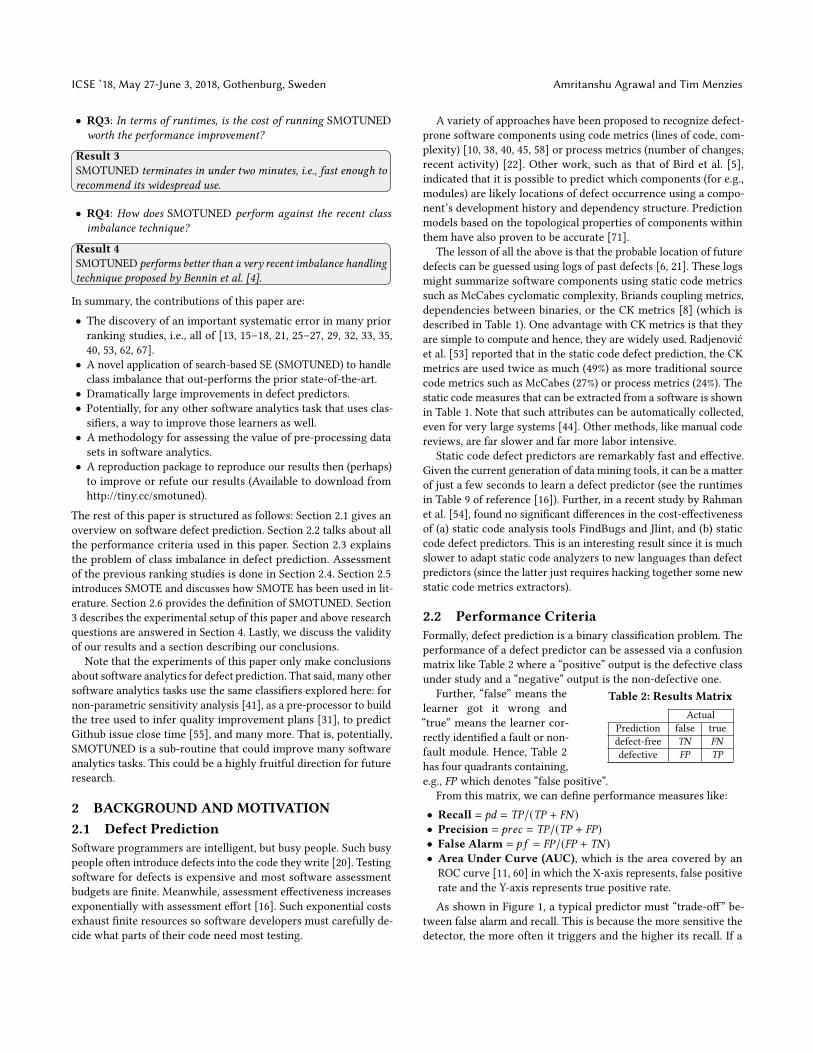
are collected from many classifiers executed on many softwaredefect data sets [13, 16–18, 21, 25–27, 29, 32, 33, 35, 40, 53, 62, 67].This section assesses those ranking studies. We will say a rankingstudy is “good” if it compares multiple learners using multiple datasets and multiple evaluation criteria while at the same time doingsomething to address the data imbalance problem.

Figure 2: Summary of Table 4.

In July 2017, we searchedscholar.google.com forthe conjunction of “soft-ware” and “defect predic-tion” and “OO” and “CK”published in the lastdecade. This returned231 results. We only se-lected OO and CK key-words since CK metricsare more popular andbetter than process met-rics for software defect prediction [53]. From that list, we selected“highly-cited” papers, which we defined as having more than 10citations per year. This reduced our population of papers downto 107. After reading the titles and abstracts of those papers, andskimming the contents of the potentially interesting papers, wefound 22 papers of Table 4 that either performed ranking studies(as defined above) or studied the effects of class imbalance on defectprediction. In the column “evaluated using multiple criteria”, papers

scored more than “1” if they used multiple performance scores ofthe kind listed at the end of Section 2.2.

We find that, in those 22 papers from Table 4, numerous classi-fiers have used AUC as the measure to evaluate the software defectpredictor studies. We also found that majority of papers (from lastcolumn of Table 4, 6/7=85%) in SE community has used SMOTE tofix the data imbalance [4, 28, 49, 50, 61, 67]. This also made us topropose SMOTUNED. As noted in [17, 32], no single classificationtechnique always dominates. That said, Table IX of a recent studyby Ghotra et al. [17] ranks numerous classifiers using data similarto what we use here (i.e., OO JAVA systems described using CKmetrics). Using their work, we can select a range of classifiers forthis study ranking from “best” to “worst’: see Table 3.

The key observation to be made from this survey is that, asshown in Figure 2, the overwhelming majority of prior papers inour sample do not satisfy our definition of a “good” project (the soleexception is the recent Bennin et al. [4] which we explore in RQ4).Accordingly, the rest of this paper defines and executes a “good”ranking study, with an additional unique feature of an auto-tuningversion of SMOTE.

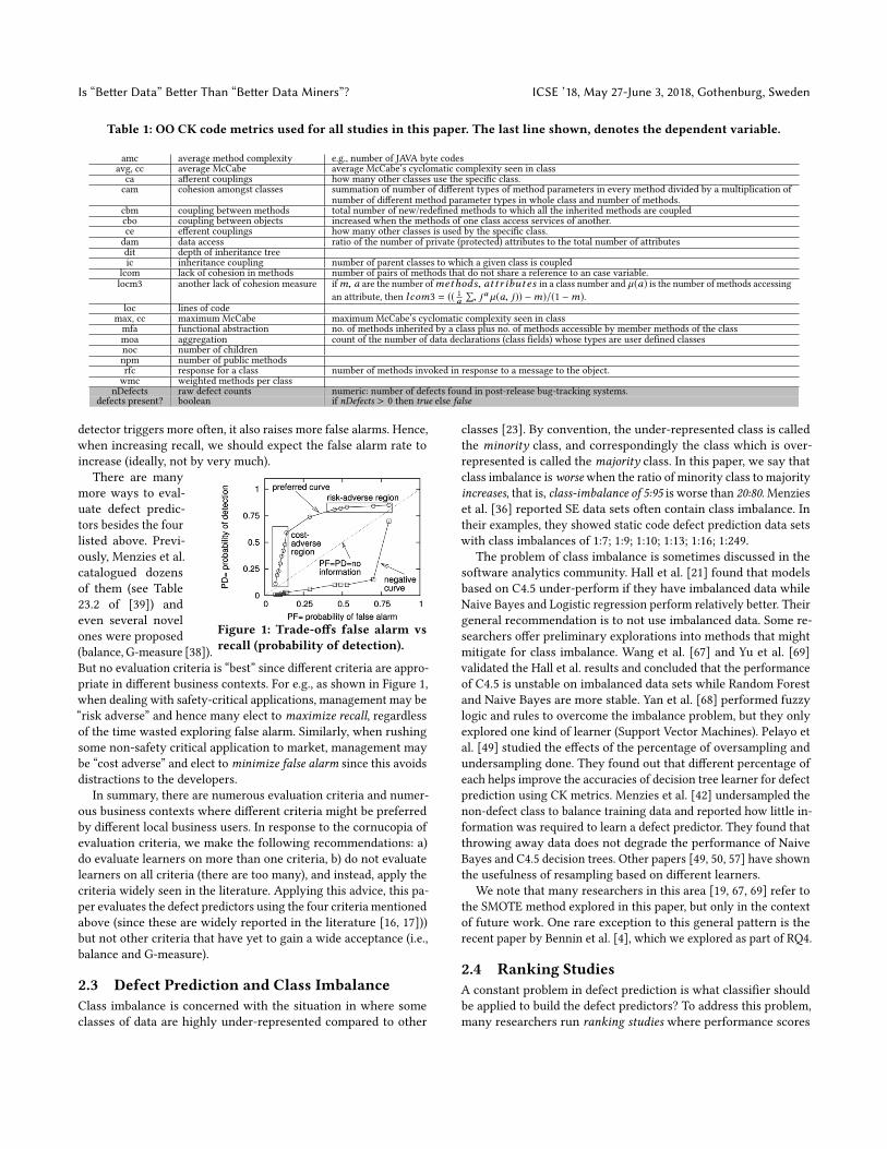
2.5 Handling Data Imbalance with SMOTESMOTE handles class imbalance by changing the frequency ofdifferent classes of the training data [7]. The algorithm’s nameis short for “synthetic minority over-sampling technique”. Whenapplied to data, SMOTE sub-samples the majority class (i.e., deletessome examples) while super-sampling the minority class until allclasses have the same frequency. In the case of software defect data,the minority class is usually the defective class.

def SMOTE(k=2,m=50%, r=2): # defaultswhile Majority > m dodelete any majority item # random

while Minority < m doadd something_like(any minority item)

def something_like(X0):relevant = emptySetk1 = 0while(k1++ < 20 and size(found) < k) {

all = k1 nearest neighborsrelevant += items in "all" of X0 class}

Z = any of foundY = interpolate (X0, Z)return Y

def minkowski_distance(a,b,r):return (Σi abs(ai − bi )r )1/r

Figure 3: Pseudocode of SMOTE

Figure 3 showshow SMOTE works.During super-sampling,a member of the mi-nority class finds knearest neighbors. Itbuilds an artificialmember of the mi-nority class at somepoint in-between it-self and one of itsrandomnearest neigh-bors. During thatprocess, some dis-tance function is re-quired which is theminkowski_distance function.

SMOTE’s control parameters are (a) k that selects how manyneighbors to use (defaults to k = 5), (b)m is how many examples of


each class which need to be generated (defaults tom = 50% of thetotal training samples), and (3) r which selects the distance function(default is r = 2, i.e., use Euclidean distance).

In the software analytics literature, there are contradictory find-ings on the value of applying SMOTE for software defect prediction.Van et al. [64], Pears et al. [47] and Tan et al. [61] found SMOTE tobe advantageous, while others, such as Pelayo et al. [49] did not.

Further, some researchers report that some learners respond bet-ter than others to SMOTE. Kamei et al. [28] evaluated the effects ofSMOTE applied to four fault-proneness models (linear discriminantanalysis, logistic regression, neural network, and decision tree) byusing two module sets of industry legacy software. They reportedthat SMOTE improved the prediction performance of the linear andlogistic models, but not neural network and decision tree models.Similar results, that the value of SMOTE was dependent on thelearner, was also reported by Van et al. [64].

Recently, Bennin et al. [4] proposed a new method based on thechromosomal theory of inheritance. Their MAHAKIL algorithminterprets two distinct sub-classes as parents and generates a newsynthetic instance that inherits different traits from each parentand contributes to the diversity within the data distribution. Theyreport that MAHAKIL usually performs as well as SMOTE, butdoes much better than all other class balancing techniques in termsof recall. Please note, that work did not consider the impact ofparameter tuning of a preprocessor so in our RQ4 we will compareSMOTUNED to MAHAKIL.

2.6 SMOTUNED = auto-tuning SMOTEOne possible explanation for the variability in the SMOTE resultsis that the default parameters of this algorithm are not suited toall data sets. To test this, we designed SMOTUNED, which is anauto-tuning version of SMOTE. SMOTUNED uses different controlparameters for different data sets.

SMOTUNED uses DE (differential evolution [59]) to explore theparameter space of Table 5. DE is an optimizer useful for functionsthat may not be smooth or linear. Vesterstrom et al. [65] find DE’soptimizations to be competitive with other optimizers like particleswarm optimization or genetic algorithms. DEs have been usedbefore for parameter tuning [2, 9, 14, 16, 46]) but this paper isthe first attempt to do DE-based class re-balancing for SE data bystudying multiple learners for multiple evaluation criteria.

In Figure 4, DE evolves a frontier of candidates from an ini-tial population which is driven by a goal (like maximizing recall)evaluated using a fitness function (shown in line 17). In the caseof SMOTUNED, each candidate is a randomly selected value forSMOTE’s k,m and r parameters. To evolve the frontier, within eachgeneration, DE compares each item to a new candidate generatedby combining three other frontier items (and better new candidatesreplace older items). To compare them, the better function (line17) calls SMOTE function (from Figure 3) using the proposed newparameter settings. This pre-processed training data is then fedinto a classifier to find a particular measure (like recall). When ourDE terminates, it returns the best candidate ever seen in the entirerun.

Table 6 provides important terms of SMOTUNED when explor-ing SMOTE’s parameter ranges, shown in Table 5. To define theparameters, we found the range of used settings for SMOTE and

1def DE( n=10, cf=0.3, f=0.7): # default settings2frontier = sets of guesses (n=10)3best = frontier.1 # any value at all4lives = 15while(lives−− > 0):6tmp = empty7for i = 1 to |frontier |: # size of frontier8old = frontieri9x,y,z = any three from frontier, picked at random10new= copy(old)11for j = 1 to |new |: # for all attributes12if rand() < cf # at probability cf...13new.j = x .j + f ∗ (z .j − y .j) # ...change item j14# end for15new = new if better(new,old) else old16tmpi = new17if better(new,best) then18best = new19lives++ # enable one more generation20end21# end for22frontier = tmp23# end while24return best

Figure 4: SMOTUNED uses DE (differential evolution).

Table 5: SMOTE parameters

ParaDefaultsused bySMOTE

Tuning Range(Explored by( SMOTUNED)

Description

k 5 [1,20] Number of neighborsm 50% {50, 100, 200, 400} Number of synthetic examples to

create. Expressed as a percent offinal training data.

r 2 [0.1,5] Power parameter for theMinkowski distance metric.

Table 6: Important Terms of SMOTUNED Algorithm

Keywords DescriptionDifferential weight (f = 0.7) Mutation power

Crossover probability (cf = 0.3) Survival of the candidatePopulation Size (n = 10) Frontier size in a generation

Lives Number of generationsFitness Function (better ) Driving factor of DE

Rand() function Returns between 0 to 1Best (or Output) Optimal configuration for SMOTE

distance functions in the SE and machine learning literature. Toavoid introducing noise by overpopulating the minority sampleswe are not usingm as percentage rather than number of examplesto create. Aggarawal et al. [1] argue that with data being highlydimensional, r should shrink to some fraction less than one (hencethe bound of r = 0.1 in Table 5).

3 EXPERIMENTAL DESIGNThis experiment reports the effects on defect prediction after usingMAHAKIL or SMOTUNED or SMOTE. Using some data Di ∈ D,performance measure Mi ∈ M , and classifier Ci ∈ C , this experi-ment conducts the 5*5 cross-validation study, defined below. Ourdata sets D are shown in Table 7. These are all open source JAVAOO systems described in terms of the CK metrics. Since, we arecomparing these results for imbalanced class, only imbalanced classdata sets were selected from SEACRAFT (http://tiny.cc/seacraft).

Our performance measures M were introduced in Section 2.2which includes AUC, precision, recall, and the false alarm. Our

http://tiny.cc/seacraft


classifiersC come from a recent study [17] andwere listed in Table 3.For implementations of these learners, we used the open sourcetool Scikit-Learn [48]. Our cross-validation study [56] is defined asfollows:(1) We randomized the order of the data set Di five times. This

reduces the probability that some random ordering of examplesin the data will conflate our results.

(2) Each time, we divided the data Di into five bins;(3) For each bin (the test), we trained on four bins (the rest) and

then tested on the test bin as follows.(a) The training set is pre-filtered using either No-SMOTE (i.e.,

do nothing) or SMOTE or SMOTUNED.(b) When using SMOTUNED, we further divide those four bins

of training data. 3 bins are used for training the model, and1 bin is used for validation in DE. DE is run to improvethe performance measure Mi seen when the classifier Ciwas applied to the training data. Important point: we onlyused SMOTE on the training data, leaving the testing dataunchanged.

(c) After pre-filtering, a classifier Ci learns a predictor.(d) The model is applied to the test data to collect performance

measureMi .(e) We print the relative performance delta between thisMi and

anotherMi generated from applying Ci to the raw data Di(i.e., compare the learner without any filtering). We finallyreport median on the 25 repeats.

Note that the above rig tunes SMOTE, but not the control pa-rameters of the classifiers. We do this since, in this paper, we aim todocument the benefits of tuning SMOTE since as shown below, theyare very large indeed. Also, it would be very useful if we can showthat a single algorithm (SMOTUNED) improves the performance ofdefect prediction. This would allow subsequent work to focus onthe task of optimizing SMOTUNED (which would be a far easiertask than optimizing the tuning of a wide-range of classifiers).

3.1 Within- vs Cross-Measure AssessmentWe call the above rig as the within-measure assessment rig since itis biased in its evaluation measures. Specifically, in this rig, whenSMOTUNED is optimized for (e.g.,) AUC, we do not explore theeffects on (e.g.,) the false alarm. This is less than ideal since it is

Table 7: Data set statistics. Data sets are sorted from low per-centage of defective class to high defective class. Data comesfrom the SEACRAFT repository: http://tiny.cc/seacraft

.Version Dataset Name Defect % No. of classes lines of code4.3 jEdit 2 492 202,3631.0 Camel 4 339 33,721

6.0.3 Tomcat 9 858 300,6742.0 Ivy 11 352 87,7691.0 Arcilook 11.5 234 31,3421.0 Redaktor 15 176 59,2801.7 Apache Ant 22 745 208,6531.2 Synapse 33.5 256 53,500

1.6.1 Velocity 34 229 57,012total: 3,681 1,034,314

known that our performance measures are inter-connected viathe Zhang’s equation [70]. Hence, increasing (e.g.,) recall mightpotentially have the adverse effect of driving up (e.g) the falsealarm rate. To avoid this problem, we also apply the following cross-measure assessment rig. At the conclusion of the within-measureassessment rig, we will observe that the AUC performance measurewill show the largest improvements. Using that best performer, wewill re-apply steps 1,2,3 abcde (listed above) but this time:• In step 3b, we will tell SMOTUNED to optimize for AUC;• In step 3d, 3e we will collect the performance delta on AUC aswell as precision, recall, and false alarm.

In this approach, steps 3d and 3e collect the information required tocheck if succeeding according to one performance criteria resultsin damage to another. We would also want to make sure that ourmodel is not over-fitted based on one evaluation measure. Andsince SMOTUNED is a time expensive task, we do not want to tunefor each measure which will quadruple the time. The results ofwithin- vs cross-measure assessment is shown in Section 4.

3.2 Statistical AnalysisWhen comparing the results of SMOTUNED to other treatments, weuse a statistical significance test and an effect size test. Significancetest are useful for detecting if two populations differ merely byrandom noise. Also, effect sizes are useful for checking that twopopulations differ by more than just a trivial amount.

For the significance test, we used the Scott-Knott procedure [17,43]. This technique recursively bi-clusters a sorted set of numbers.If any two clusters are statistically indistinguishable, Scott-Knottreports them both as one group. Scott-Knott first looks for a breakin the sequence that maximizes the expected values in the differencein the means before and after the break. More specifically, it splitsl values into sub-listsm and n in order to maximize the expectedvalue of differences in the observed performances before and afterdivisions. For e.g., lists l ,m and n of size ls,ms and ns where l =m∪n, Scott-Knott divides the sequence at the break that maximizes:

E(∆) =ms/ls ∗ abs(m.µ − l .µ)2 + ns/ls ∗ abs(n.µ − l .µ)2

Scott-Knott then applies some statistical hypothesis test H to checkif m and n are significantly different. If so, Scott-Knott then re-curses on each division. For this study, our hypothesis test H was aconjunction of the A12 effect size test (endorsed by [3]) and non-parametric bootstrap sampling [12], i.e., our Scott-Knott dividedthe data if both bootstrapping and an effect size test agreed thatthe division was statistically significant (99% confidence) and not a“small” effect (A12 ≥ 0.6).

4 RESULTSRQ1: Are the default “off-the-shelf” parameters for SMOTEappropriate for all data sets?

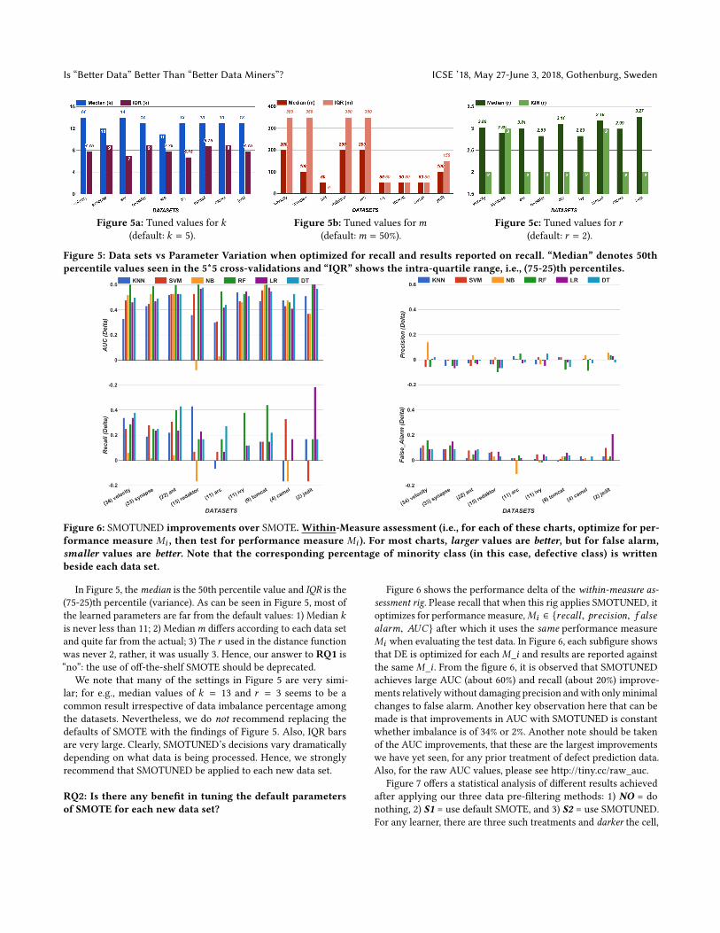
As discussed above, the default parameters for SMOTE, k, mand r are 5, 50% and 2. Figure 5 shows the range of parametersfound by SMOTUNED across nine data sets for the 25 repeatsof our cross-validation procedure. All the results in this figureare within-measure assessment results, i.e., here, we SMOTUNEDon a particular performance measure and then we only collectperformance for that performance measure on the test set.


Figure 5a: Tuned values for k(default: k = 5).

Figure 5b: Tuned values form(default:m = 50%).

Figure 5c: Tuned values for r(default: r = 2).

Figure 5: Data sets vs Parameter Variation when optimized for recall and results reported on recall. “Median” denotes 50thpercentile values seen in the 5*5 cross-validations and “IQR” shows the intra-quartile range, i.e., (75-25)th percentiles.

Figure 6: SMOTUNED improvements over SMOTE. Within-Measure assessment (i.e., for each of these charts, optimize for per-formance measure Mi , then test for performance measure Mi ). For most charts, larger values are better, but for false alarm,smaller values are better. Note that the corresponding percentage of minority class (in this case, defective class) is writtenbeside each data set.

In Figure 5, themedian is the 50th percentile value and IQR is the(75-25)th percentile (variance). As can be seen in Figure 5, most ofthe learned parameters are far from the default values: 1) Median kis never less than 11; 2) Medianm differs according to each data setand quite far from the actual; 3) The r used in the distance functionwas never 2, rather, it was usually 3. Hence, our answer to RQ1 is“no”: the use of off-the-shelf SMOTE should be deprecated.

We note that many of the settings in Figure 5 are very simi-lar; for e.g., median values of k = 13 and r = 3 seems to be acommon result irrespective of data imbalance percentage amongthe datasets. Nevertheless, we do not recommend replacing thedefaults of SMOTE with the findings of Figure 5. Also, IQR barsare very large. Clearly, SMOTUNED’s decisions vary dramaticallydepending on what data is being processed. Hence, we stronglyrecommend that SMOTUNED be applied to each new data set.

RQ2: Is there any benefit in tuning the default parametersof SMOTE for each new data set?

Figure 6 shows the performance delta of the within-measure as-sessment rig. Please recall that when this rig applies SMOTUNED, itoptimizes for performance measure,Mi ∈ {recall , precision, f alsealarm, AUC} after which it uses the same performance measureMi when evaluating the test data. In Figure 6, each subfigure showsthat DE is optimized for eachM_i and results are reported againstthe sameM_i . From the figure 6, it is observed that SMOTUNEDachieves large AUC (about 60%) and recall (about 20%) improve-ments relatively without damaging precision andwith onlyminimalchanges to false alarm. Another key observation here that can bemade is that improvements in AUC with SMOTUNED is constantwhether imbalance is of 34% or 2%. Another note should be takenof the AUC improvements, that these are the largest improvementswe have yet seen, for any prior treatment of defect prediction data.Also, for the raw AUC values, please see http://tiny.cc/raw_auc.

Figure 7 offers a statistical analysis of different results achievedafter applying our three data pre-filtering methods: 1) NO = donothing, 2) S1 = use default SMOTE, and 3) S2 = use SMOTUNED.For any learner, there are three such treatments and darker the cell,

http://tiny.cc/raw_auc


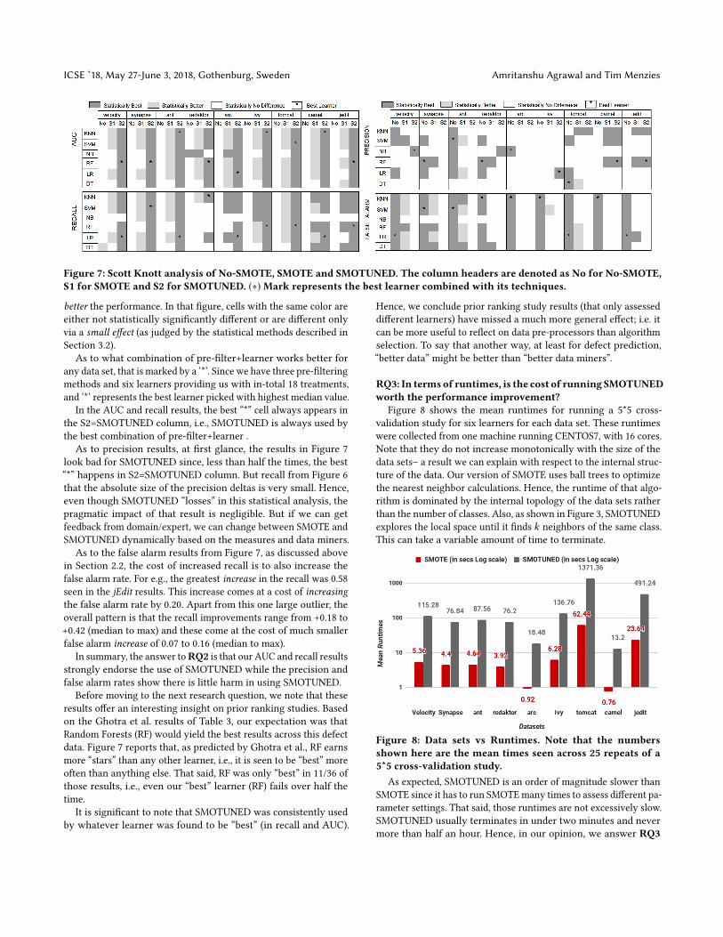
Figure 7: Scott Knott analysis of No-SMOTE, SMOTE and SMOTUNED. The column headers are denoted as No for No-SMOTE,S1 for SMOTE and S2 for SMOTUNED. (∗) Mark represents the best learner combined with its techniques.

better the performance. In that figure, cells with the same color areeither not statistically significantly different or are different onlyvia a small effect (as judged by the statistical methods described inSection 3.2).

As to what combination of pre-filter+learner works better forany data set, that is marked by a ‘*’. Since we have three pre-filteringmethods and six learners providing us with in-total 18 treatments,and ‘*’ represents the best learner picked with highest median value.

In the AUC and recall results, the best “*” cell always appears inthe S2=SMOTUNED column, i.e., SMOTUNED is always used bythe best combination of pre-filter+learner .

As to precision results, at first glance, the results in Figure 7look bad for SMOTUNED since, less than half the times, the best“*” happens in S2=SMOTUNED column. But recall from Figure 6that the absolute size of the precision deltas is very small. Hence,even though SMOTUNED “losses” in this statistical analysis, thepragmatic impact of that result is negligible. But if we can getfeedback from domain/expert, we can change between SMOTE andSMOTUNED dynamically based on the measures and data miners.

As to the false alarm results from Figure 7, as discussed abovein Section 2.2, the cost of increased recall is to also increase thefalse alarm rate. For e.g., the greatest increase in the recall was 0.58seen in the jEdit results. This increase comes at a cost of increasingthe false alarm rate by 0.20. Apart from this one large outlier, theoverall pattern is that the recall improvements range from +0.18 to+0.42 (median to max) and these come at the cost of much smallerfalse alarm increase of 0.07 to 0.16 (median to max).

In summary, the answer toRQ2 is that our AUC and recall resultsstrongly endorse the use of SMOTUNED while the precision andfalse alarm rates show there is little harm in using SMOTUNED.

Before moving to the next research question, we note that theseresults offer an interesting insight on prior ranking studies. Basedon the Ghotra et al. results of Table 3, our expectation was thatRandom Forests (RF) would yield the best results across this defectdata. Figure 7 reports that, as predicted by Ghotra et al., RF earnsmore “stars” than any other learner, i.e., it is seen to be “best” moreoften than anything else. That said, RF was only “best” in 11/36 ofthose results, i.e., even our “best” learner (RF) fails over half thetime.

It is significant to note that SMOTUNED was consistently usedby whatever learner was found to be “best” (in recall and AUC).

Hence, we conclude prior ranking study results (that only assesseddifferent learners) have missed a much more general effect; i.e. itcan be more useful to reflect on data pre-processors than algorithmselection. To say that another way, at least for defect prediction,“better data” might be better than “better data miners”.

RQ3: In terms of runtimes, is the cost of running SMOTUNEDworth the performance improvement?

Figure 8 shows the mean runtimes for running a 5*5 cross-validation study for six learners for each data set. These runtimeswere collected from one machine running CENTOS7, with 16 cores.Note that they do not increase monotonically with the size of thedata sets– a result we can explain with respect to the internal struc-ture of the data. Our version of SMOTE uses ball trees to optimizethe nearest neighbor calculations. Hence, the runtime of that algo-rithm is dominated by the internal topology of the data sets ratherthan the number of classes. Also, as shown in Figure 3, SMOTUNEDexplores the local space until it finds k neighbors of the same class.This can take a variable amount of time to terminate.

Figure 8: Data sets vs Runtimes. Note that the numbersshown here are the mean times seen across 25 repeats of a5*5 cross-validation study.

As expected, SMOTUNED is an order of magnitude slower thanSMOTE since it has to run SMOTEmany times to assess different pa-rameter settings. That said, those runtimes are not excessively slow.SMOTUNED usually terminates in under two minutes and nevermore than half an hour. Hence, in our opinion, we answer RQ3


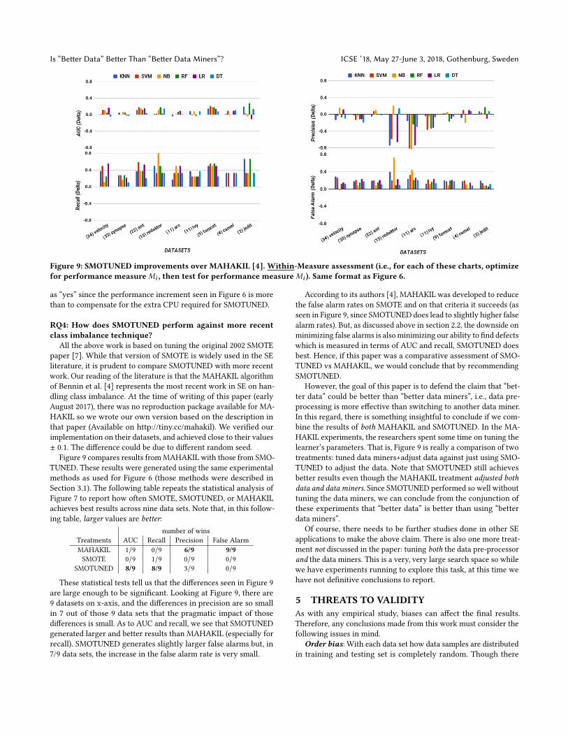
Figure 9: SMOTUNED improvements over MAHAKIL [4]. Within-Measure assessment (i.e., for each of these charts, optimizefor performance measureMi , then test for performance measureMi ). Same format as Figure 6.

as “yes” since the performance increment seen in Figure 6 is morethan to compensate for the extra CPU required for SMOTUNED.

RQ4: How does SMOTUNED perform against more recentclass imbalance technique?

All the above work is based on tuning the original 2002 SMOTEpaper [7]. While that version of SMOTE is widely used in the SEliterature, it is prudent to compare SMOTUNED with more recentwork. Our reading of the literature is that the MAHAKIL algorithmof Bennin et al. [4] represents the most recent work in SE on han-dling class imbalance. At the time of writing of this paper (earlyAugust 2017), there was no reproduction package available for MA-HAKIL so we wrote our own version based on the description inthat paper (Available on http://tiny.cc/mahakil). We verified ourimplementation on their datasets, and achieved close to their values± 0.1. The difference could be due to different random seed.

Figure 9 compares results fromMAHAKIL with those from SMO-TUNED. These results were generated using the same experimentalmethods as used for Figure 6 (those methods were described inSection 3.1). The following table repeats the statistical analysis ofFigure 7 to report how often SMOTE, SMOTUNED, or MAHAKILachieves best results across nine data sets. Note that, in this follow-ing table, larger values are better:

number of winsTreatments AUC Recall Precision False AlarmMAHAKIL 1/9 0/9 6/9 9/9SMOTE 0/9 1/9 0/9 0/9

SMOTUNED 8/9 8/9 3/9 0/9

These statistical tests tell us that the differences seen in Figure 9are large enough to be significant. Looking at Figure 9, there are9 datasets on x-axis, and the differences in precision are so smallin 7 out of those 9 data sets that the pragmatic impact of thosedifferences is small. As to AUC and recall, we see that SMOTUNEDgenerated larger and better results than MAHAKIL (especially forrecall). SMOTUNED generates slightly larger false alarms but, in7/9 data sets, the increase in the false alarm rate is very small.

According to its authors [4], MAHAKIL was developed to reducethe false alarm rates on SMOTE and on that criteria it succeeds (asseen in Figure 9, since SMOTUNED does lead to slightly higher falsealarm rates). But, as discussed above in section 2.2, the downside onminimizing false alarms is also minimizing our ability to find defectswhich is measured in terms of AUC and recall, SMOTUNED doesbest. Hence, if this paper was a comparative assessment of SMO-TUNED vs MAHAKIL, we would conclude that by recommendingSMOTUNED.

However, the goal of this paper is to defend the claim that “bet-ter data” could be better than “better data miners”, i.e., data pre-processing is more effective than switching to another data miner.In this regard, there is something insightful to conclude if we com-bine the results of both MAHAKIL and SMOTUNED. In the MA-HAKIL experiments, the researchers spent some time on tuning thelearner’s parameters. That is, Figure 9 is really a comparison of twotreatments: tuned data miners+adjust data against just using SMO-TUNED to adjust the data. Note that SMOTUNED still achievesbetter results even though the MAHAKIL treatment adjusted bothdata and data miners. Since SMOTUNED performed so well withouttuning the data miners, we can conclude from the conjunction ofthese experiments that “better data” is better than using “betterdata miners”.

Of course, there needs to be further studies done in other SEapplications to make the above claim. There is also one more treat-ment not discussed in the paper: tuning both the data pre-processorand the data miners. This is a very, very large search space so whilewe have experiments running to explore this task, at this time wehave not definitive conclusions to report.

5 THREATS TO VALIDITYAs with any empirical study, biases can affect the final results.Therefore, any conclusions made from this work must consider thefollowing issues in mind.

Order bias: With each data set how data samples are distributedin training and testing set is completely random. Though there

http://tiny.cc/mahakil


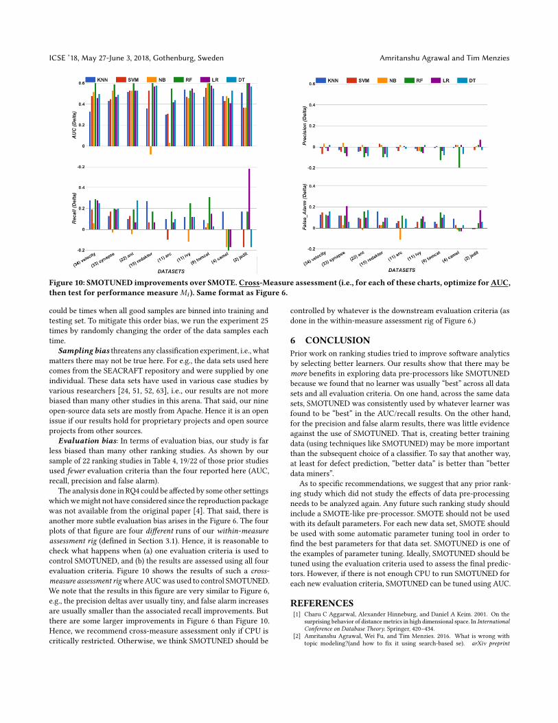
Figure 10: SMOTUNED improvements over SMOTE. Cross-Measure assessment (i.e., for each of these charts, optimize for AUC,then test for performance measureMi ). Same format as Figure 6.

could be times when all good samples are binned into training andtesting set. To mitigate this order bias, we run the experiment 25times by randomly changing the order of the data samples eachtime.

Sampling bias threatens any classification experiment, i.e., whatmatters there may not be true here. For e.g., the data sets used herecomes from the SEACRAFT repository and were supplied by oneindividual. These data sets have used in various case studies byvarious researchers [24, 51, 52, 63], i.e., our results are not morebiased than many other studies in this arena. That said, our nineopen-source data sets are mostly from Apache. Hence it is an openissue if our results hold for proprietary projects and open sourceprojects from other sources.

Evaluation bias: In terms of evaluation bias, our study is farless biased than many other ranking studies. As shown by oursample of 22 ranking studies in Table 4, 19/22 of those prior studiesused fewer evaluation criteria than the four reported here (AUC,recall, precision and false alarm).

The analysis done in RQ4 could be affected by some other settingswhichwemight not have considered since the reproduction packagewas not available from the original paper [4]. That said, there isanother more subtle evaluation bias arises in the Figure 6. The fourplots of that figure are four different runs of our within-measureassessment rig (defined in Section 3.1). Hence, it is reasonable tocheck what happens when (a) one evaluation criteria is used tocontrol SMOTUNED, and (b) the results are assessed using all fourevaluation criteria. Figure 10 shows the results of such a cross-measure assessment rigwhereAUCwas used to control SMOTUNED.We note that the results in this figure are very similar to Figure 6,e.g., the precision deltas aver usually tiny, and false alarm increasesare usually smaller than the associated recall improvements. Butthere are some larger improvements in Figure 6 than Figure 10.Hence, we recommend cross-measure assessment only if CPU iscritically restricted. Otherwise, we think SMOTUNED should be

controlled by whatever is the downstream evaluation criteria (asdone in the within-measure assessment rig of Figure 6.)

6 CONCLUSIONPrior work on ranking studies tried to improve software analyticsby selecting better learners. Our results show that there may bemore benefits in exploring data pre-processors like SMOTUNEDbecause we found that no learner was usually “best” across all datasets and all evaluation criteria. On one hand, across the same datasets, SMOTUNED was consistently used by whatever learner wasfound to be “best” in the AUC/recall results. On the other hand,for the precision and false alarm results, there was little evidenceagainst the use of SMOTUNED. That is, creating better trainingdata (using techniques like SMOTUNED) may be more importantthan the subsequent choice of a classifier. To say that another way,at least for defect prediction, “better data” is better than “betterdata miners”.

As to specific recommendations, we suggest that any prior rank-ing study which did not study the effects of data pre-processingneeds to be analyzed again. Any future such ranking study shouldinclude a SMOTE-like pre-processor. SMOTE should not be usedwith its default parameters. For each new data set, SMOTE shouldbe used with some automatic parameter tuning tool in order tofind the best parameters for that data set. SMOTUNED is one ofthe examples of parameter tuning. Ideally, SMOTUNED should betuned using the evaluation criteria used to assess the final predic-tors. However, if there is not enough CPU to run SMOTUNED foreach new evaluation criteria, SMOTUNED can be tuned using AUC.

REFERENCES[1] Charu C Aggarwal, Alexander Hinneburg, and Daniel A Keim. 2001. On the

surprising behavior of distance metrics in high dimensional space. In InternationalConference on Database Theory. Springer, 420–434.

[2] Amritanshu Agrawal, Wei Fu, and Tim Menzies. 2016. What is wrong withtopic modeling?(and how to fix it using search-based se). arXiv preprint


arXiv:1608.08176 (2016).[3] Andrea Arcuri and Lionel Briand. 2011. A practical guide for using statistical tests

to assess randomized algorithms in software engineering. In Software Engineering(ICSE), 2011 33rd International Conference on. IEEE, 1–10.

[4] Kwabena Ebo Bennin, Jacky Keung, Passakorn Phannachitta, Akito Monden, andSolomon Mensah. 2017. MAHAKIL: Diversity based Oversampling Approachto Alleviate the Class Imbalance Issue in Software Defect Prediction. IEEETransactions on Software Engineering (2017).

[5] Christian Bird, Nachiappan Nagappan, Harald Gall, Brendan Murphy, andPremkumar Devanbu. 2009. Putting it all together: Using socio-technical net-works to predict failures. In 2009 20th ISSRE. IEEE, 109–119.

[6] Cagatay Catal and Banu Diri. 2009. A systematic review of software fault predic-tion studies. Expert systems with applications 36, 4 (2009), 7346–7354.

[7] Nitesh V. Chawla, Kevin W. Bowyer, Lawrence O. Hall, and W. Philip Kegelmeyer.2002. SMOTE: synthetic minority over-sampling technique. Journal of artificialintelligence research 16 (2002), 321–357.

[8] Shyam R Chidamber and Chris F Kemerer. 1994. A metrics suite for objectoriented design. IEEE Transactions on software engineering 20, 6 (1994), 476–493.

[9] I. Chiha, J. Ghabi, and N. Liouane. 2012. Tuning PID controller with multi-objective differential evolution. In ISCCSP ’12. IEEE, 1–4.

[10] Marco D’Ambros, Michele Lanza, and Romain Robbes. 2010. An extensive com-parison of bug prediction approaches. In 2010 7th IEEE MSR). IEEE, 31–41.

[11] Richard O Duda, Peter E Hart, and David G Stork. 2012. Pattern classification.John Wiley & Sons.

[12] Bradley Efron and Robert J Tibshirani. 1994. An introduction to the bootstrap.Chapman and Hall, London.

[13] Karim O Elish and Mahmoud O Elish. 2008. Predicting defect-prone softwaremodules using support vector machines. JSS 81, 5 (2008), 649–660.

[14] Wei Fu and Tim Menzies. 2017. Easy over Hard: A Case Study on Deep Learning.arXiv preprint arXiv:1703.00133 (2017).

[15] Wei Fu and Tim Menzies. 2017. Revisiting unsupervised learning for defectprediction. In Proceedings of the 2017 11th Joint Meeting on Foundations of SoftwareEngineering. ACM, 72–83.

[16] Wei Fu, Tim Menzies, and Xipeng Shen. 2016. Tuning for software analytics: Is itreally necessary? IST 76 (2016), 135–146.

[17] Baljinder Ghotra, Shane McIntosh, and Ahmed E Hassan. 2015. Revisiting the im-pact of classification techniques on the performance of defect prediction models.In 37th ICSE-Volume 1. IEEE Press, 789–800.

[18] Iker Gondra. 2008. Applying machine learning to software fault-pronenessprediction. Journal of Systems and Software 81, 2 (2008), 186–195.

[19] David Gray, David Bowes, Neil Davey, Yi Sun, and Bruce Christianson. 2009.Using the support vector machine as a classification method for software defectprediction with static code metrics. In International Conference on EngineeringApplications of Neural Networks. Springer, 223–234.

[20] Philip J Guo, Thomas Zimmermann, NachiappanNagappan, and BrendanMurphy.2011. Not my bug! and other reasons for software bug report reassignments. InProceedings of the ACM 2011 conference on Computer supported cooperative work.ACM, 395–404.

[21] Tracy Hall, Sarah Beecham, David Bowes, David Gray, and Steve Counsell. 2012.A systematic literature review on fault prediction performance in software engi-neering. IEEE TSE 38, 6 (2012), 1276–1304.

[22] Ahmed E Hassan. 2009. Predicting faults using the complexity of code changes.In 31st ICSE. IEEE Computer Society, 78–88.

[23] Haibo He and Edwardo A Garcia. 2009. Learning from imbalanced data. IEEETransactions on knowledge and data engineering 21, 9 (2009), 1263–1284.

[24] Zhimin He, Fengdi Shu, Ye Yang, Mingshu Li, and Qing Wang. 2012. An investi-gation on the feasibility of cross-project defect prediction. Automated SoftwareEngineering 19, 2 (2012), 167–199.

[25] Yue Jiang, Bojan Cukic, and Yan Ma. 2008. Techniques for evaluating faultprediction models. Empirical Software Engineering 13, 5 (2008), 561–595.

[26] Yue Jiang, Bojan Cukic, and Tim Menzies. 2008. Can data transformation helpin the detection of fault-prone modules?. In Proceedings of the 2008 workshop onDefects in large software systems. ACM, 16–20.

[27] Yue Jiang, Jie Lin, Bojan Cukic, and Tim Menzies. 2009. Variance analysis in soft-ware fault prediction models. In Software Reliability Engineering, 2009. ISSRE’09.20th International Symposium on. IEEE, 99–108.

[28] Yasutaka Kamei, Akito Monden, Shinsuke Matsumoto, Takeshi Kakimoto, andKen-ichi Matsumoto. 2007. The effects of over and under sampling on fault-pronemodule detection. In ESEM 2007. IEEE, 196–204.

[29] Taghi M Khoshgoftaar, Kehan Gao, and Naeem Seliya. 2010. Attribute selectionand imbalanced data: Problems in software defect prediction. In Tools with Artifi-cial Intelligence (ICTAI), 2010 22nd IEEE International Conference on, Vol. 1. IEEE,137–144.

[30] Sunghun Kim, Hongyu Zhang, Rongxin Wu, and Liang Gong. 2011. Dealing withnoise in defect prediction. In Software Engineering (ICSE), 2011 33rd InternationalConference on. IEEE, 481–490.

[31] Rahul Krishna, Tim Menzies, and Lucas Layman. 2017. Less is More: MinimizingCode Reorganization using XTREE. Information and Software Technology (2017).

[32] Stefan Lessmann, Bart Baesens, Christophe Mues, and Swantje Pietsch. 2008.Benchmarking classification models for software defect prediction: A proposedframework and novel findings. IEEE TSE 34, 4 (2008), 485–496.

[33] Ming Li, Hongyu Zhang, Rongxin Wu, and Zhi-Hua Zhou. 2012. Sample-basedsoftware defect prediction with active and semi-supervised learning. AutomatedSoftware Engineering 19, 2 (2012), 201–230.

[34] Michael Lowry, Mark Boyd, and Deepak Kulkami. 1998. Towards a theory forintegration of mathematical verification and empirical testing. In AutomatedSoftware Engineering, 1998. Proceedings. 13th IEEE International Conference on.IEEE, 322–331.

[35] Thilo Mende and Rainer Koschke. 2009. Revisiting the evaluation of defectprediction models. In Proceedings of the 5th International Conference on PredictorModels in Software Engineering. ACM, 7.

[36] Tim Menzies, Alex Dekhtyar, Justin Distefano, and Jeremy Greenwald. 2007.Problems with Precision: A Response to" comments on’data mining static codeattributes to learn defect predictors’". IEEE TSE 33, 9 (2007).

[37] Tim Menzies and Justin S. Di Stefano. 2004. How Good is Your Blind SpotSampling Policy. In Proceedings of the Eighth IEEE International Conference on HighAssurance Systems Engineering (HASE’04). IEEE Computer Society, Washington,DC, USA, 129–138. http://dl.acm.org/citation.cfm?id=1890580.1890593

[38] Tim Menzies, Jeremy Greenwald, and Art Frank. 2007. Data mining static codeattributes to learn defect predictors. IEEE TSE 33, 1 (2007), 2–13.

[39] Tim Menzies, Ekrem Kocaguneli, Burak Turhan, Leandro Minku, and FayolaPeters. 2014. Sharing data and models in software engineering. Morgan Kaufmann.

[40] TimMenzies, ZachMilton, Burak Turhan, Bojan Cukic, Yue Jiang, and Ayşe Bener.2010. Defect prediction from static code features: current results, limitations,new approaches. Automated Software Engineering 17, 4 (2010), 375–407.

[41] Tim Menzies and Erik Sinsel. 2000. Practical large scale what-if queries: Casestudies with software risk assessment. In Automated Software Engineering, 2000.Proceedings ASE 2000. The Fifteenth IEEE International Conference on. IEEE, 165–173.

[42] Tim Menzies, Burak Turhan, Ayse Bener, Gregory Gay, Bojan Cukic, and YueJiang. 2008. Implications of ceiling effects in defect predictors. In Proceedings ofthe 4th international workshop on Predictor models in software engineering. ACM,47–54.

[43] Nikolaos Mittas and Lefteris Angelis. 2013. Ranking and clustering software costestimation models through a multiple comparisons algorithm. IEEE Transactionson software engineering 39, 4 (2013), 537–551.

[44] Nachiappan Nagappan and Thomas Ball. 2005. Static analysis tools as earlyindicators of pre-release defect density. In Proceedings of the 27th internationalconference on Software engineering. ACM, 580–586.

[45] Nachiappan Nagappan, Thomas Ball, and Andreas Zeller. 2006. Mining metricsto predict component failures. In Proceedings of the 28th international conferenceon Software engineering. ACM, 452–461.

[46] M. Omran, A. P. Engelbrecht, and A. Salman. 2005. Differential evolution methodsfor unsupervised image classification. In IEEE Congress on Evolutionary Compu-tation ’05, Vol. 2. 966–973.

[47] Russel Pears, Jacqui Finlay, and Andy M Connor. 2014. Synthetic Minority over-sampling technique (SMOTE) for predicting software build outcomes. arXivpreprint arXiv:1407.2330 (2014).

[48] Fabian Pedregosa, Gaël Varoquaux, Alexandre Gramfort, Vincent Michel,Bertrand Thirion, Olivier Grisel, Mathieu Blondel, Peter Prettenhofer, Ron Weiss,Vincent Dubourg, and others. 2011. Scikit-learn: Machine learning in Python.Journal of Machine Learning Research 12, Oct (2011), 2825–2830.

[49] Lourdes Pelayo and Scott Dick. 2007. Applying novel resampling strategies tosoftware defect prediction. In NAFIPS 2007-2007 Annual Meeting of the NorthAmerican Fuzzy Information Processing Society. IEEE, 69–72.

[50] Lourdes Pelayo and Scott Dick. 2012. Evaluating stratification alternatives toimprove software defect prediction. IEEE Transactions on Reliability 61, 2 (2012),516–525.

[51] Fayola Peters, Tim Menzies, Liang Gong, and Hongyu Zhang. 2013. Balancingprivacy and utility in cross-company defect prediction. IEEE Transactions onSoftware Engineering 39, 8 (2013), 1054–1068.

[52] Fayola Peters, Tim Menzies, and Andrian Marcus. 2013. Better cross companydefect prediction. In Mining Software Repositories (MSR), 2013 10th IEEE WorkingConference on. IEEE, 409–418.

[53] Danijel Radjenović, Marjan Heričko, Richard Torkar, and Aleš Živkovič. 2013.Software fault prediction metrics: A systematic literature review. Informationand Software Technology 55, 8 (2013), 1397–1418.

[54] Foyzur Rahman, Sameer Khatri, Earl T. Barr, and Premkumar Devanbu. 2014.Comparing Static Bug Finders and Statistical Prediction (ICSE). ACM, New York,NY, USA, 424–434. DOI:http://dx.doi.org/10.1145/2568225.2568269

[55] Mitch Rees-Jones, Matthew Martin, and Tim Menzies. 2017. Better Predictors forIssue Lifetime. CoRR abs/1702.07735 (2017). http://arxiv.org/abs/1702.07735

[56] Payam Refaeilzadeh, Lei Tang, and Huan Liu. 2009. Cross-validation. In Encyclo-pedia of database systems. Springer, 532–538.

[57] JC Riquelme, R Ruiz, D Rodríguez, and J Moreno. 2008. Finding defective modulesfrom highly unbalanced datasets. Actas de los Talleres de las Jornadas de Ingeniería

http://dl.acm.org/citation.cfm?id=1890580.1890593

http://dx.doi.org/10.1145/2568225.2568269

http://arxiv.org/abs/1702.07735


del Software y Bases de Datos 2, 1 (2008), 67–74.[58] Martin Shepperd, David Bowes, and Tracy Hall. 2014. Researcher bias: The use

of machine learning in software defect prediction. IEEE Transactions on SoftwareEngineering 40, 6 (2014), 603–616.

[59] Rainer Storn and Kenneth Price. 1997. Differential evolution–a simple andefficient heuristic for global optimization over continuous spaces. Journal ofglobal optimization 11, 4 (1997), 341–359.

[60] John A Swets. 1988. Measuring the accuracy of diagnostic systems. Science 240,4857 (1988), 1285.

[61] Ming Tan, Lin Tan, Sashank Dara, and Caleb Mayeux. 2015. Online defectprediction for imbalanced data. In ICSE-Volume 2. IEEE Press, 99–108.

[62] Chakkrit Tantithamthavorn, Shane McIntosh, Ahmed E Hassan, and KenichiMatsumoto. 2016. Automated parameter optimization of classification techniquesfor defect prediction models. In ICSE 2016. ACM, 321–332.

[63] Burak Turhan, Ayşe Tosun Mısırlı, and Ayşe Bener. 2013. Empirical evaluationof the effects of mixed project data on learning defect predictors. Informationand Software Technology 55, 6 (2013), 1101–1118.

[64] Jason Van Hulse, Taghi M Khoshgoftaar, and Amri Napolitano. 2007. Experi-mental perspectives on learning from imbalanced data. In Proceedings of the 24thinternational conference on Machine learning. ACM, 935–942.

[65] Jakob Vesterstrom and Rene Thomsen. 2004. A comparative study of differentialevolution, particle swarm optimization, and evolutionary algorithms on numeri-cal benchmark problems. In Evolutionary Computation, 2004. CEC2004. Congresson, Vol. 2. IEEE, 1980–1987.

[66] Jeffrey M. Voas and Keith W Miller. 1995. Software testability: The new verifica-tion. IEEE software 12, 3 (1995), 17–28.

[67] ShuoWang and Xin Yao. 2013. Using class imbalance learning for software defectprediction. IEEE Transactions on Reliability 62, 2 (2013), 434–443.

[68] Zhen Yan, Xinyu Chen, and Ping Guo. 2010. Software defect prediction usingfuzzy support vector regression. In International Symposium on Neural Networks.Springer, 17–24.

[69] Qiao Yu, Shujuan Jiang, and Yanmei Zhang. 2017. The Performance Stabilityof Defect Prediction Models with Class Imbalance: An Empirical Study. IEICETRANSACTIONS on Information and Systems 100, 2 (2017), 265–272.

[70] Hongyu Zhang and Xiuzhen Zhang. 2007. Comments on Data Mining Static CodeAttributes to Learn Defect Predictors. IEEE Transactions on Software Engineering33, 9 (2007), 635–637.

[71] Thomas Zimmermann and Nachiappan Nagappan. 2008. Predicting defects usingnetwork analysis on dependency graphs. In ICSE. ACM, 531–540.

is “better data” better than “better data miners”? · is “better data” better than...

Documents