is high-frequency trading inducing changes in … · is high-frequency trading inducing changes in...
TRANSCRIPT
Electronic copy available at: http://ssrn.com/abstract=1632077
Is high-frequency trading inducing changes inmarket microstructure and dynamics?
Reginald SmithPO Box 10051, Rochester, NY 14610
E-mail: [email protected]
Abstract. Using high-frequency time series of stock prices and share volumessizes from January 2002-May 2009, this paper investigates whether the effects ofthe onset of high-frequency trading, most prominent since 2005, are apparent inthe dynamics of the dollar traded volume. Indeed it is found in almost all of 14heavily traded stocks, that there has been an increase in the Hurst exponent ofdollar traded volume from Gaussian noise in the earlier years to more self-similardynamics in later years. This shift is linked both temporally to the Reg NMSreforms allowing high-frequency trading to flourish as well as to the decliningaverage size of trades with smaller trades showing markedly higher degrees ofself-similarity.
Keywords: financial markets, algorithmic trading, self-similarity, wavelets, highfrequency trading, Hurst exponent
Electronic copy available at: http://ssrn.com/abstract=1632077
Is high-frequency trading inducing changes in market microstructure and dynamics?2
1. Introduction
Over the last couple of decades, cheap computing power and improvedtelecommunications have all but obsoleted to old style open-cry auctions which droveequity markets for centuries. This change has occurred so rapidly, that it has disruptedthe traditional dominance of the exchanges, brought into finance new strategies such asstatistical arbitrage, and fuelled intense public and regulatory debate over the positivebenefits and costs of the new world of electronic trading.
One of the largest effects of this movement has been the disruption of andcontroversy about old paradigms such as assumed normal distributions of asset returnsand the absence of long-term persistence in price fluctuations that random walk modelsdictate. However, recent advances in data analysis techniques and recent financialmarket turbulence may provide a fertile proving ground for research that improvesboth a theoretical and empirical understanding of financial market dynamics.
The field of research which has likely attracted some of the largest attention andliterature in quantitative finance and econophysics Mantegna and Stanley (1999);Tsay (2002) is likely the research of the movements by asset prices and volumesin trading on financial markets. This is for several reasons. First, the data, whichare fundamentally time series amongst correlated systems, are amenable to the well-developed techniques from econometrics, physical research, and applied mathematicsand statistics. Second, large datasets are easily and cheaply available, sometimesfor free, as in the case of daily closing prices. Combined with cheap computingpower, there is a low barrier to entry for participants eager to apply many well-knowntechniques to price dynamics of stocks, currencies, or other widely traded assets.
A common theme in this research has often been the investigation of self-similarityand long-range dependence in the time series. The former is often measured by theHurst exponent, H, which measures the relative degree of self-similarity from pureMarkovian Browninan motion at H = 0.5 to complete self-similarity at H = 1. Avalue of 0.5 < H < 1 is typically described by fractional Brownian motion whichdemonstrates self-similarity at multiple time scales of fluctuations in contrast tothe independent fluctuations of Brownian motion. Self-similarity and long-rangedependence in financial time series has a long and sometimes contentious history.There are many papers disputing whether the most common measure, log assetreturns, display any sort of self-similarity which would bring the efficient markethypothesis into questions Lo (1991); Lobato and Savin (1998); Grau-Carles (2005)Studies on trading volume Lobato and Velasco (2000); Liesenfeld (2002) or tradedvalue seem tend to demonstrate H > 0.5 over long time scales. One key exception,however, tends to be short term intraday equity trading data. In particular, in Eisleret. al. (2005); Eisler and Kertesz (2007a,b) intraday trading dollar value, on theorder of times less than 60 minutes, universally demonstrate H ≈ 0.5 indicating thereexists different scaling behavior at different time scales for equity trading volumes. Forlong periods of intraday trading or trades across multiple days, there is almost alwaysa significant deviation from Gaussian noise and H > 0.5. Therefore, traditionally thecorrelation structure of trading time series is generated at time scales of the ordersof many minutes or hours and is not an inherent feature of the dynamics at shortertimescales.
This paper is organized as follows. First, a brief introduction to the history offinancial markets in the in the US will be given which culminates in the reforms ofthe late 20th and early 21st century which enabled high frequency trading. Next, the
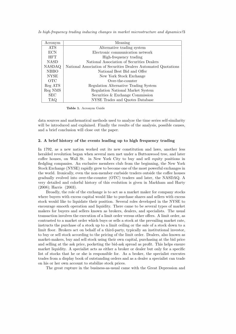
Is high-frequency trading inducing changes in market microstructure and dynamics?3
Acronym MeaningATS Alternative trading systemECN Electronic communication networkHFT High-frequency trading
NASD National Association of Securities DealersNASDAQ National Association of Securities Dealers Automated Quotations
NBBO National Best Bid and OfferNYSE New York Stock ExchangeOTC Over-the-counter
Reg ATS Regulation Alternative Trading SystemReg NMS Regulation National Market System
SEC Securities & Exchange CommissionTAQ NYSE Trades and Quotes Database
Table 1. Acronym Guide
data sources and mathematical methods used to analyze the time series self-similaritywill be introduced and explained. Finally the results of the analysis, possible causes,and a brief conclusion will close out the paper.
2. A brief history of the events leading up to high frequency trading
In 1792, as a new nation worked out its new constitution and laws, another lessheralded revolution began when several men met under a Buttonwood tree, and latercoffee houses, on Wall St. in New York City to buy and sell equity positions infledgling companies. An exclusive members club from the beginning, the New YorkStock Exchange (NYSE) rapidly grew to become one of the most powerful exchanges inthe world. Ironically, even the non-member curbside traders outside the coffee housesgradually evolved into over-the-counter (OTC) traders and later, the NASDAQ. Avery detailed and colorful history of this evolution is given in Markham and Harty(2008); Harris (2003).
Broadly, the role of the exchange is to act as a market maker for company stockswhere buyers with excess capital would like to purchase shares and sellers with excessstock would like to liquidate their position. Several roles developed in the NYSE toencourage smooth operation and liquidity. There came to be several types of marketmakers for buyers and sellers known as brokers, dealers, and specialists. The usualtransaction involves the execution of a limit order versus other offers. A limit order, ascontrasted to a market order which buys or sells a stock at the prevailing market rate,instructs the purchase of a stock up to a limit ceiling or the sale of a stock down to alimit floor. Brokers act on behalf of a third-party, typically an institutional investor,to buy or sell stock according to the pricing of the limit order. Dealers, also known asmarket-makers, buy and sell stock using their own capital, purchasing at the bid priceand selling at the ask price, pocketing the bid-ask spread as profit. This helps ensuremarket liquidity. A specialist acts as either a broker or dealer but only for a specificlist of stocks that he or she is responsible for. As a broker, the specialist executestrades from a display book of outstanding orders and as a dealer a specialist can tradeon his or her own account to stabilize stock prices.
The great rupture in the business-as-usual came with the Great Depression and
Is high-frequency trading inducing changes in market microstructure and dynamics?4
the unfolding revelations of corrupt stock dealings, fraud, and other such malfeasance.The Securities and Exchange Commission (SEC) was created by Congress in 1934 bythe Securities Exchange Act. Since then, it has acted as the regulator of the stockexchanges and the companies that list on them. Over time, the SEC and Wall Streethave evolved together, influencing each other in the process.
By the 1960s, the volume of traded shares was overwhelming the traditionalpaper systems that brokers, dealers, and specialists on the floor used. A“paperworkcrisis” developed that seriously hampered operations of the NYSE and led to thefirst electronic order routing system, DOT by 1976. In addition, inefficiencies inthe handling of OTC orders, also known as “pink sheets”, led to a 1963 SECrecommendation of changes to the industry which led the National Association ofSecurities Dealers (NASD) to form the NASDAQ in 1968. Orders were displayedelectronically while the deals were made through the telephone through“marketmakers” instead of dealers or specialists. In 1975, under the prompting of Congress,the SEC passed the Regulation of the National Market System, more commonlyknown as Reg NMS, which was used to mandate the interconnectedness of variousmarkets for stocks to prevent a tiered marketplace where small, medium, and largeinvestors would have a specific market and smaller investors would be disadvantaged.One of the outcomes of Reg NMS was the accelerated use of technology to connectmarkets and display quotes. This would enable stocks to be traded on different,albeit connected, exchanges from the NYSE such as the soon to emerge electroniccommunication networks (ECNs), known to the SEC as alternative trading systems(ATS).
In the 1980s, the NYSE upgraded their order system again to SuperDot. Theincreasing speed and availability computers helped enable trading of entire portfoliosof stocks simultaneously in what became known as program trading. One of the firstinstances of algorithmic trading, program trading was not high-frequency per se butused to trade large orders of multiple stocks at once. Program trading was profitablebut is now often cited as one of the largest factors behind the 1987 Black Mondaycrash. Even the human systems broke down, however, as many NASDAQ marketmakers did not answer the phones during the crash.
The true acceleration of progress and the advent of what is now known as highfrequency trading occurred during the 1990s. The telecommunications technologyboom as well as the dotcom frenzy led to many extensive changes. A new groupof exchanges became prominent. These were the ECN/ATS exchanges. Using newcomputer technology, they provided an alternate market platform where buyers andsellers could have their orders matched automatically to the best price withoutmiddlemen such as dealers or brokers. They also allowed complete anonymity forbuyers and sellers. One issue though was even though they were connected to theexchanges via Reg NMS requirements, there was little mandated transparency. Inother words, deals settled on the ECN/ATS were not revealed to the exchange. On theflip side, the exchange brokers were not obligated to transact with an order displayedfrom an ECN, even if it was better for their customer.
This began to change, partially because of revelations of multiple violations offiduciary duty by specialists in the NYSE. One example, similar to the soon to beinvented ‘flash trading’, was where they would “interposition” themselves betweentheir clients and the best offer in order to either buy low from the client and sell higherto the NBBO (National Best Bid and Offer; the best price) price or vice versa. In 1997,the SEC passed the Limit Order Display rule to improve transparency that required
Is high-frequency trading inducing changes in market microstructure and dynamics?5
market makers to include offers at better prices than those the market maker is offeringto investors. This allows investors to know the NBBO and circumvent corruption.However, this rule also had the effect of requiring the exchanges to display electronicorders from the ECN/ATS systems that were better priced. The SEC followed up in1998 with Regulation ATS. Reg ATS allowed ECN/ATS systems to register as eitherbrokers or exchanges. It also protected investors by mandating reporting requirementsand transparency of aggregate trading activity for ECN/ATS systems once they reacha certain size.
These changes opened up huge new opportunities for ECN/ATS systems byallowing them to display and execute quotes directly with the big exchanges. Thoughthey were required to report these transactions to the exchange, they gained muchmore. In particular, with their advanced technology and low-latency communicationsystems, they became a portal through which next generation algorithmic trading andhigh frequency trading algorithms could have access to wider markets. Changes stillcontinued to accelerate.
In 2000, were two other groundbreaking changes. First was the decimalization ofthe price quotes on US stocks. This reduced the bid-ask spreads and made it mucheasier for computer algorithms to trade stocks and conduct arbitrage. The NYSE alsorepealed Rule 390 which had prohibited the trading of stocks listed prior to April 26,1979 outside of the exchange. High frequency trading began to grow rapidly but didnot truly take off until 2005.
In June 2005, the SEC revised Reg NMS with several key mandates. Some wererelatively minor such as the Sub-Penny rule which prevented stock quotations at aresolution less than one cent. However, the biggest change was Rule 611, also knownas the Order Protection Rule. Whereas with the Limit Order Display rule, exchangeswere merely required to display better quotes, Reg NMS Rule 611 mandated, withsome exceptions, that trades are always automatically executed at the best quotepossible. Price is the only issue and not counterparty reliability, transaction speed,etc. The opening for high frequency trading here is clear. The automatic tradeexecution created the perfect environment for high speed transactions that would beautomatically executed and not sit in a queue waiting for approval by a market makeror some vague exchange rule. The limit to trading speed and profit was now mostlythe latency on electronic trading systems.
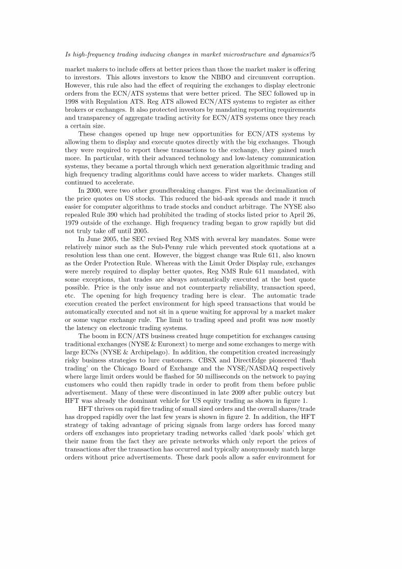
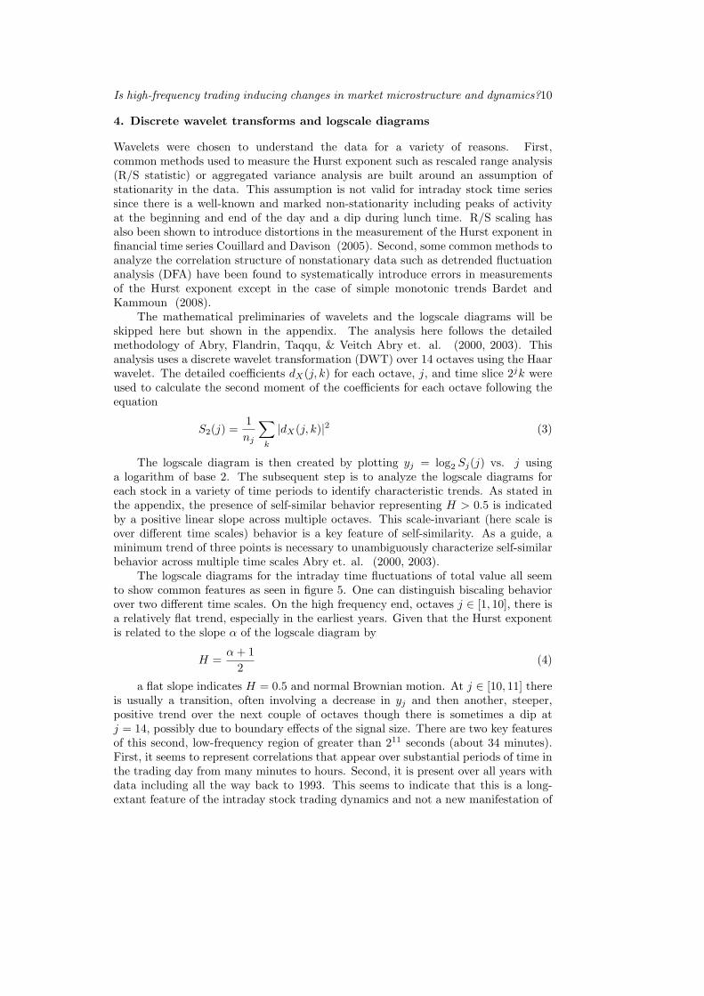
The boom in ECN/ATS business created huge competition for exchanges causingtraditional exchanges (NYSE & Euronext) to merge and some exchanges to merge withlarge ECNs (NYSE & Archipelago). In addition, the competition created increasinglyrisky business strategies to lure customers. CBSX and DirectEdge pioneered ‘flashtrading’ on the Chicago Board of Exchange and the NYSE/NASDAQ respectivelywhere large limit orders would be flashed for 50 milliseconds on the network to payingcustomers who could then rapidly trade in order to profit from them before publicadvertisement. Many of these were discontinued in late 2009 after public outcry butHFT was already the dominant vehicle for US equity trading as shown in figure 1.
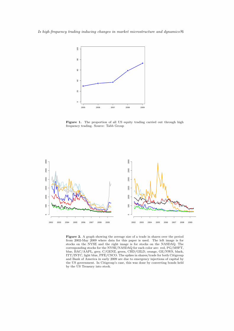
HFT thrives on rapid fire trading of small sized orders and the overall shares/tradehas dropped rapidly over the last few years is shown in figure 2. In addition, the HFTstrategy of taking advantage of pricing signals from large orders has forced manyorders off exchanges into proprietary trading networks called ‘dark pools’ which gettheir name from the fact they are private networks which only report the prices oftransactions after the transaction has occurred and typically anonymously match largeorders without price advertisements. These dark pools allow a safer environment for
Is high-frequency trading inducing changes in market microstructure and dynamics?6
2005 2006 2007 2008 2009
020
4060
8010
0
Figure 1. The proportion of all US equity trading carried out through highfrequency trading. Source: Tabb Group
2002 2003 2004 2005 2006 2007 2008 2009
050
010
0015
0020
0025
0030
00
2002 2003 2004 2005 2006 2007 2008 2009
050
010
0015
0020
0025
0030
00
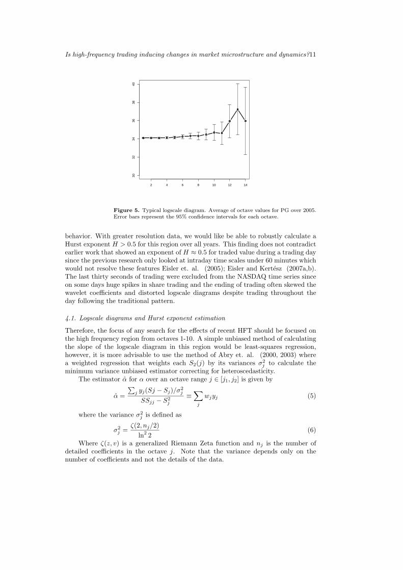
Figure 2. A graph showing the average size of a trade in shares over the periodfrom 2002-May 2009 where data for this paper is used. The left image is forstocks on the NYSE and the right image is for stocks on the NASDAQ. Thecorresponding stocks for the NYSE/NASDAQ for each color are: red, PG/MSFT,blue, BAC/AAPL, grey, C/GENZ, green, CHD/GILD, orange, GE/NWS, black,ITT/INTC, light blue, PFE/CSCO. The spikes in shares/trade for both Citigroupand Bank of America in early 2009 are due to emergency injections of capital bythe US government. In Citigroup’s case, this was done by converting bonds heldby the US Treasury into stock.
Is high-frequency trading inducing changes in market microstructure and dynamics?7
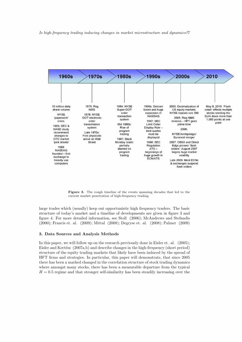
Figure 3. The rough timeline of the events spanning decades that led to thecurrent market penetration of high-frequency trading.
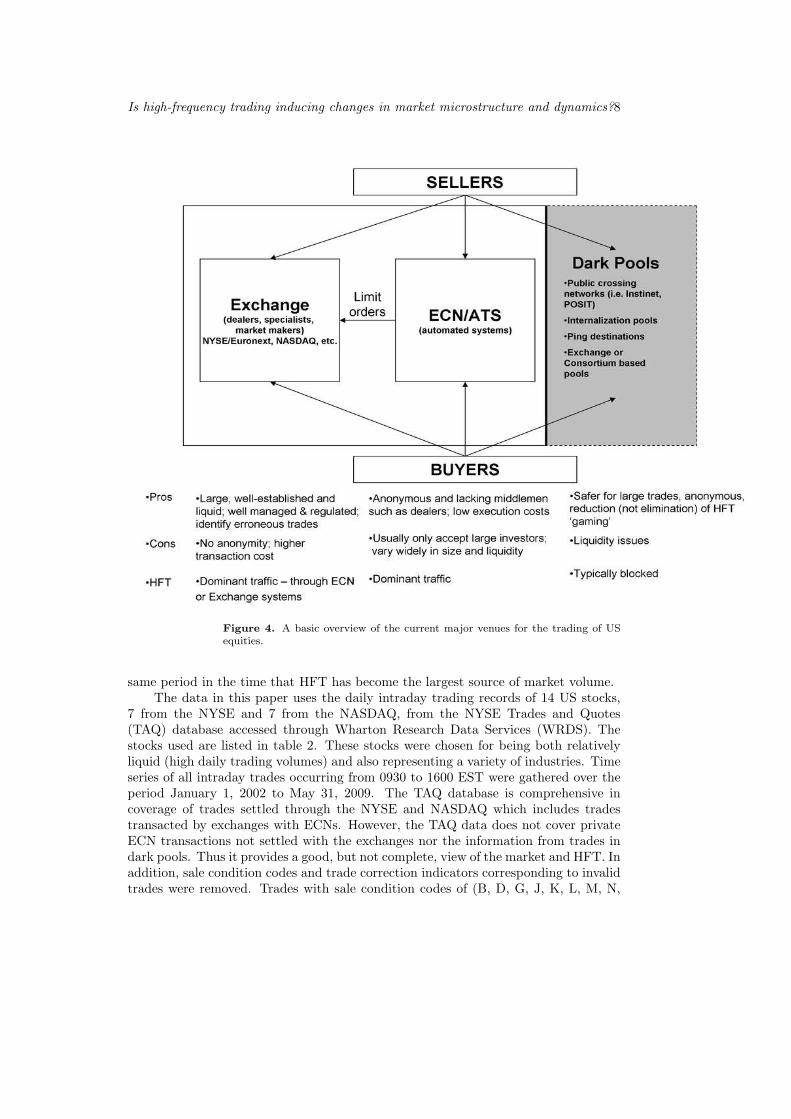
large trades which (usually) keep out opportunistic high frequency traders. The basicstructure of today’s market and a timeline of developments are given in figure 3 andfigure 4. For more detailed information, see Stoll (2006); McAndrews and Stefandis(2000); Francis et. al. (2009); Mittal (2008); Degryse et. al. (2008); Palmer (2009)
3. Data Sources and Analysis Methods
In this paper, we will follow up on the research previously done in Eisler et. al. (2005);Eisler and Kertesz (2007a,b) and describe changes in the high-frequency (short period)structure of the equity trading markets that likely have been induced by the spread ofHFT firms and strategies. In particular, this paper will demonstrate, that since 2005there has been a marked changed in the correlation structure of stock trading dynamicswhere amongst many stocks, there has been a measurable departure from the typicalH = 0.5 regime and that stronger self-similarity has been steadily increasing over the
Is high-frequency trading inducing changes in market microstructure and dynamics?8
Figure 4. A basic overview of the current major venues for the trading of USequities.
same period in the time that HFT has become the largest source of market volume.The data in this paper uses the daily intraday trading records of 14 US stocks,
7 from the NYSE and 7 from the NASDAQ, from the NYSE Trades and Quotes(TAQ) database accessed through Wharton Research Data Services (WRDS). Thestocks used are listed in table 2. These stocks were chosen for being both relativelyliquid (high daily trading volumes) and also representing a variety of industries. Timeseries of all intraday trades occurring from 0930 to 1600 EST were gathered over theperiod January 1, 2002 to May 31, 2009. The TAQ database is comprehensive incoverage of trades settled through the NYSE and NASDAQ which includes tradestransacted by exchanges with ECNs. However, the TAQ data does not cover privateECN transactions not settled with the exchanges nor the information from trades indark pools. Thus it provides a good, but not complete, view of the market and HFT. Inaddition, sale condition codes and trade correction indicators corresponding to invalidtrades were removed. Trades with sale condition codes of (B, D, G, J, K, L, M, N,
Is high-frequency trading inducing changes in market microstructure and dynamics?9
Quote Symbol Stock NameBAC Bank of America
C CiticorpPG Proctor & GambleGE General ElectricITT ITT IndustriesCHD Church & DwightPFE Pfizer
MSFT MicrosoftINTC IntelCSCO CiscoGENZ GenzymeGILD Gilead SciencesAAPL Apple Computer Inc.NWS News Corp.
Table 2. Quote symbols and stocks discussed in this paper.
O, P, Q, R, T, U, W, Z, 4 (NASDAQ), 6(NASDAQ)), trade correction indicators notequal of 0, 1, or 2, or negative share sizes or prices were excluded from calculationsby the algorithm.
Following techniques from Eisler et. al. (2005); Eisler and Kertesz (2007a,b),the measured variable is the traded value per unit time where the traded valueVi(n)for a stock i in transaction n is defined as
Vi(n) = pi(n)Si(n) (1)
where pi(n) is the price the trade is executed at and Si(n) is the share size of thetrade. The traded value per unit time ∆t is defined as
f∆ti (t) =
∑
n,ti(n)∈[t,t+∆t]
Vi(n) (2)
The trade data had a resolution of 1 second and trades were aggregated into1 second buckets for analysis of the time series. Each trading day was analyzedindependently and data was not combined across days. The first step was a briefanalysis to investigate the presence or absence of HFT via average share sizes overthe measured period. For all selected stocks, there was a marked decrease in theaverage number of shares per trade shown collectively in figure 2. This decrease intrade size was used as prima facie evidence of the influence of HFT on the selectedstocks. Next to be addressed was whether the short-term correlation structure ofintraday stock trading has been significantly affected by HFT and related strategies.All previous papers, and data pulled from NYSE TAQ on stocks in 1993 by the author,indicate that short-term correlations were traditionally largely absent from the tradingpatterns, consistently showing an average H ≈ 0.5.
In order to fully investigate the structure of intraday trading over several timescales at many orders of magnitude, a discrete wavelet transform was used to create alogscale diagram to observe the behavior of the second moment of the detailed waveletcoefficients across multiple octaves representing different time scales. A brief overviewof the wavelet analysis is given in the appendix and the logscale diagram in describedin the next section.
Is high-frequency trading inducing changes in market microstructure and dynamics?10
4. Discrete wavelet transforms and logscale diagrams
Wavelets were chosen to understand the data for a variety of reasons. First,common methods used to measure the Hurst exponent such as rescaled range analysis(R/S statistic) or aggregated variance analysis are built around an assumption ofstationarity in the data. This assumption is not valid for intraday stock time seriessince there is a well-known and marked non-stationarity including peaks of activityat the beginning and end of the day and a dip during lunch time. R/S scaling hasalso been shown to introduce distortions in the measurement of the Hurst exponent infinancial time series Couillard and Davison (2005). Second, some common methods toanalyze the correlation structure of nonstationary data such as detrended fluctuationanalysis (DFA) have been found to systematically introduce errors in measurementsof the Hurst exponent except in the case of simple monotonic trends Bardet andKammoun (2008).
The mathematical preliminaries of wavelets and the logscale diagrams will beskipped here but shown in the appendix. The analysis here follows the detailedmethodology of Abry, Flandrin, Taqqu, & Veitch Abry et. al. (2000, 2003). Thisanalysis uses a discrete wavelet transformation (DWT) over 14 octaves using the Haarwavelet. The detailed coefficients dX(j, k) for each octave, j, and time slice 2jk wereused to calculate the second moment of the coefficients for each octave following theequation
S2(j) =1nj
∑
k
|dX(j, k)|2 (3)
The logscale diagram is then created by plotting yj = log2 Sj(j) vs. j usinga logarithm of base 2. The subsequent step is to analyze the logscale diagrams foreach stock in a variety of time periods to identify characteristic trends. As stated inthe appendix, the presence of self-similar behavior representing H > 0.5 is indicatedby a positive linear slope across multiple octaves. This scale-invariant (here scale isover different time scales) behavior is a key feature of self-similarity. As a guide, aminimum trend of three points is necessary to unambiguously characterize self-similarbehavior across multiple time scales Abry et. al. (2000, 2003).
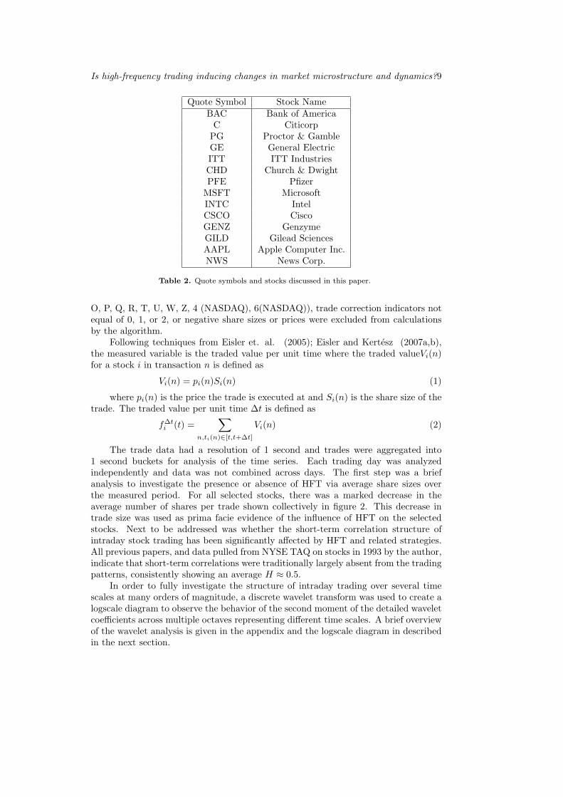
The logscale diagrams for the intraday time fluctuations of total value all seemto show common features as seen in figure 5. One can distinguish biscaling behaviorover two different time scales. On the high frequency end, octaves j ∈ [1, 10], there isa relatively flat trend, especially in the earliest years. Given that the Hurst exponentis related to the slope α of the logscale diagram by
H =α + 1
2(4)
a flat slope indicates H = 0.5 and normal Brownian motion. At j ∈ [10, 11] thereis usually a transition, often involving a decrease in yj and then another, steeper,positive trend over the next couple of octaves though there is sometimes a dip atj = 14, possibly due to boundary effects of the signal size. There are two key featuresof this second, low-frequency region of greater than 211 seconds (about 34 minutes).First, it seems to represent correlations that appear over substantial periods of time inthe trading day from many minutes to hours. Second, it is present over all years withdata including all the way back to 1993. This seems to indicate that this is a long-extant feature of the intraday stock trading dynamics and not a new manifestation of
Is high-frequency trading inducing changes in market microstructure and dynamics?11
2 4 6 8 10 12 14
3032
3436
3840
Figure 5. Typical logscale diagram. Average of octave values for PG over 2005.Error bars represent the 95% confidence intervals for each octave.
behavior. With greater resolution data, we would like be able to robustly calculate aHurst exponent H > 0.5 for this region over all years. This finding does not contradictearlier work that showed an exponent of H ≈ 0.5 for traded value during a trading daysince the previous research only looked at intraday time scales under 60 minutes whichwould not resolve these features Eisler et. al. (2005); Eisler and Kertesz (2007a,b).The last thirty seconds of trading were excluded from the NASDAQ time series sinceon some days huge spikes in share trading and the ending of trading often skewed thewavelet coefficients and distorted logscale diagrams despite trading throughout theday following the traditional pattern.
4.1. Logscale diagrams and Hurst exponent estimation
Therefore, the focus of any search for the effects of recent HFT should be focused onthe high frequency region from octaves 1-10. A simple unbiased method of calculatingthe slope of the logscale diagram in this region would be least-squares regression,however, it is more advisable to use the method of Abry et. al. (2000, 2003) wherea weighted regression that weights each S2(j) by its variances σ2
j to calculate theminimum variance unbiased estimator correcting for heteroscedasticity.
The estimator α for α over an octave range j ∈ [j1, j2] is given by
α =
∑j yj(Sj − Sj)/σ2
j
SSjj − S2j
≡∑
j
wjyj (5)
where the variance σ2j is defined as
σ2j =
ζ(2, nj/2)ln2 2
(6)
Where ζ(z, v) is a generalized Riemann Zeta function and nj is the number ofdetailed coefficients in the octave j. Note that the variance depends only on thenumber of coefficients and not the details of the data.
Is high-frequency trading inducing changes in market microstructure and dynamics?12
The additional variables are defined S =∑
[j1,j2](1/σ2
j ), Sj =∑
[j1,j2](j/σ2
j ) andSjj =
∑[j1,j2]
(j2/σ2j ). Note the S variables must be calculated before the summation
in the full estimator equation. Additionally, the variance of α is given by
V ar(α) =∑
j
σ2j w2
j (7)
The distribution of α, can be considered approximately Gaussian and using twostandard deviations for 95% confidence intervals, the 95% confidence interval of α±0.02 and given equation 4, the 95% confidence interval of calculated daily H is±0.01.
5. Results of wavelet analysis
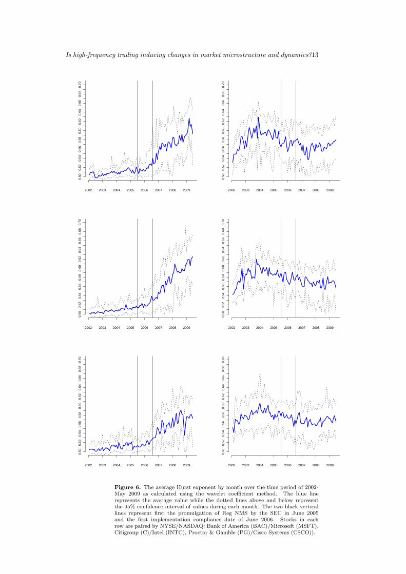
Calculations of H according to the above methodology were done for each stock oneach day over the time periods of the data. In order to more easily visualize trends,H was averaged over each month and plotted over time from January 2002 to May2009. The following pages show the figures for monthly averages of the trends for eachstock over time with 95% confidence intervals, given the range of measured H overthe month, given by dashed lines. The two vertical solid lines give the passing of theReg NMS changes and their first implementation deadline respectively.
The first clear feature is a trend across all stocks for the time periods shown.For the NYSE stocks, the Hurst exponents increase from 2002 onward but by late2005 barely break the average of H = 0.55. Therefore, during this time (and before),short term trading fluctuations do not appreciably depart from an approximation ofGaussian white noise. However, once Reg NMS is implemented the structure of thetrading noise begins to change rapidly increasing to 0.6 and beyond in a couple ofyears. This is a new behavior in the high-frequency spectrum of trading data thatindicates increasingly correlated trading activity over increasingly shorter timescalesover the last several years. Correlations previously only seen across hours or days intrading time series are increasingly showing up in the timescales of seconds or minutes.
A more complicated picture is shown in the NASDAQ data. The Hurst exponentof NASDAQ stocks started rising much earlier, from 2002 or earlier. By the timeReg NMS was passed, most NASDAQ stocks already had an H which many stockson the NYSE would not reach until 2009. Some NASDAQ stocks, such as AAPL orCSCO, did have spikes shortly after the new rules went into effect but soon returnedto normal behavior. In fact, data from Figure 10 shows this spike for AAPL was likelynot due to HFT as it was most pronounced amongst larger sized trades. It is probablethat since NASDAQ was one of the first exchanges to embrace electronic trading andexperience HFT via ECNs, the rules officially unchaining HFT for other exchangesfrom 2005 was close to a non-event. Possibly, because HFT was experienced earlier,there is not as dramatic a rise from the time of Reg NMS in H for NASDAQ. The onemarked change from the implementation time of Reg NMS is the emergence of massiveshare trades at the final seconds of trading days, sometimes varying over many ordersof magnitude by day, that required the time series to remove to get clear data.
In order to more clearly understand the source of the increased self-similarity inthe trading noise, the data was analyzed again in buckets corresponding to tradesof a certain size. In all cases it was found that the H of trades where the averageshares/trade was greater than about 1500 shares had an H ≈ 0.5 for all time periodswhile H > 0.5 for trades with an average of less than 1500 shares per trade. The
Is high-frequency trading inducing changes in market microstructure and dynamics?13
0.50
0.52
0.54
0.56
0.58
0.60
0.62
0.64
0.66
0.68
0.70
2002 2003 2004 2005 2006 2007 2008 2009 2002 2003 2004 2005 2006 2007 2008 2009
0.50
0.52
0.54
0.56
0.58
0.60
0.62
0.64
0.66
0.68
0.70
2002 2003 2004 2005 2006 2007 2008 2009
0.50
0.52
0.54
0.56
0.58
0.60
0.62
0.64
0.66
0.68
0.70
0.50
0.52
0.54
0.56
0.58
0.60
0.62
0.64
0.66
0.68
0.70
2002 2003 2004 2005 2006 2007 2008 2009
2002 2003 2004 2005 2006 2007 2008 2009
0.50
0.52
0.54
0.56
0.58
0.60
0.62
0.64
0.66
0.68
0.70
2002 2003 2004 2005 2006 2007 2008 2009
0.50
0.52
0.54
0.56
0.58
0.60
0.62
0.64
0.66
0.68
0.70
Figure 6. The average Hurst exponent by month over the time period of 2002-May 2009 as calculated using the wavelet coefficient method. The blue linerepresents the average value while the dotted lines above and below representthe 95% confidence interval of values during each month. The two black verticallines represent first the promulgation of Reg NMS by the SEC in June 2005and the first implementation compliance date of June 2006. Stocks in eachrow are paired by NYSE/NASDAQ: Bank of America (BAC)/Microsoft (MSFT),Citigroup (C)/Intel (INTC), Proctor & Gamble (PG)/Cisco Systems (CSCO)).

Is high-frequency trading inducing changes in market microstructure and dynamics?14
0.50
0.52
0.54
0.56
0.58
0.60
0.62
0.64
0.66
0.68
0.70
2002 2003 2004 2005 2006 2007 2008 2009
0.50
0.52
0.54
0.56
0.58
0.60
0.62
0.64
0.66
0.68
0.70
2002 2003 2004 2005 2006 2007 2008 2009
2002 2003 2004 2005 2006 2007 2008 2009
0.50
0.52
0.54
0.56
0.58
0.60
0.62
0.64
0.66
0.68
0.70
2002 2003 2004 2005 2006 2007 2008 2009
0.50
0.52
0.54
0.56
0.58
0.60
0.62
0.64
0.66
0.68
0.70
2002 2003 2004 2005 2006 2007 2008 2009
0.50
0.52
0.54
0.56
0.58
0.60
0.62
0.64
0.66
0.68
0.70
0.50
0.52
0.54
0.56
0.58
0.60
0.62
0.64
0.66
0.68
0.70
2002 2003 2004 2005 2006 2007 2008 2009
Figure 7. The average Hurst exponent by month over the time period of 2002-May 2009 as calculated using the wavelet coefficient method. The blue linerepresents the average value while the dotted lines above and below represent the95% confidence interval of values during each month. The two black vertical linesrepresent first the promulgation of Reg NMS by the SEC in June 2005 and thefirst implementation compliance date of June 2006. Stocks in each row are pairedby NYSE/NASDAQ: General Electric (GE)/Apple Computer (AAPL), ITTIndustries (ITT)/Genzyme (GENZ), Church & Dwight (CHD)/Gilead Sciences(GILD).
Is high-frequency trading inducing changes in market microstructure and dynamics?15
0.50
0.52
0.54
0.56
0.58
0.60
0.62
0.64
0.66
0.68
0.70
2002 2003 2004 2005 2006 2007 2008 2009 2002 2003 2004 2005 2006 2007 2008 2009
0.50
0.52
0.54
0.56
0.58
0.60
0.62
0.64
0.66
0.68
0.70
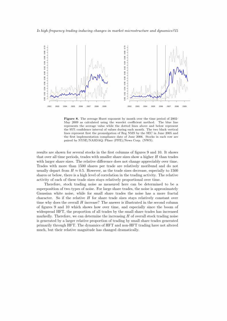
Figure 8. The average Hurst exponent by month over the time period of 2002-May 2009 as calculated using the wavelet coefficient method. The blue linerepresents the average value while the dotted lines above and below representthe 95% confidence interval of values during each month. The two black verticallines represent first the promulgation of Reg NMS by the SEC in June 2005 andthe first implementation compliance date of June 2006. Stocks in each row arepaired by NYSE/NASDAQ: Pfizer (PFE)/News Corp. (NWS).
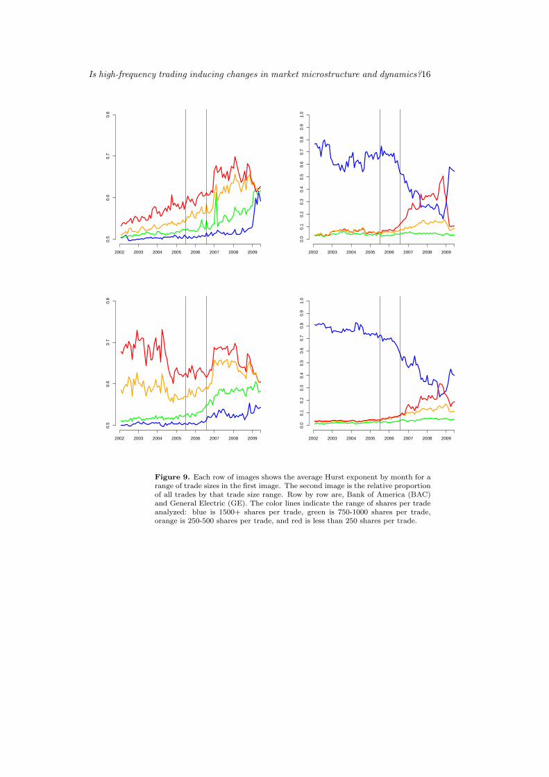
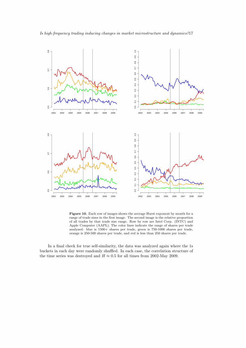
results are shown for several stocks in the first columns of figures 9 and 10. It showsthat over all time periods, trades with smaller share sizes show a higher H than tradeswith larger share sizes. The relative difference does not change appreciably over time.Trades with more than 1500 shares per trade are relatively moribund and do notusually depart from H ≈ 0.5. However, as the trade sizes decrease, especially to 1500shares or below, there is a high level of correlation in the trading activity. The relativeactivity of each of these trade sizes stays relatively proportional over time.
Therefore, stock trading noise as measured here can be determined to be asuperposition of two types of noise. For large share trades, the noise is approximatelyGaussian white noise, while for small share trades the noise has a more fractalcharacter. So if the relative H for share trade sizes stays relatively constant overtime why does the overall H increase? The answer is illustrated in the second columnof figures 9 and 10 which shows how over time, and especially since the boom ofwidespread HFT, the proportion of all trades by the small share trades has increasedmarkedly. Therefore, we can determine the increasing H of overall stock trading noiseis generated by a larger relative proportion of trading by small share trades generatedprimarily through HFT. The dynamics of HFT and non-HFT trading have not alteredmuch, but their relative magnitude has changed dramatically.
Is high-frequency trading inducing changes in market microstructure and dynamics?16
0.5
0.6
0.7
0.8
2002 2003 2004 2005 2006 2007 2008 2009
0.0
0.1
0.2
0.3
0.4
0.5
0.6
0.7
0.8
0.9
1.0
2002 2003 2004 2005 2006 2007 2008 2009
0.5
0.6
0.7
0.8
2002 2003 2004 2005 2006 2007 2008 2009 2002 2003 2004 2005 2006 2007 2008 2009
0.0
0.1
0.2
0.3
0.4
0.5
0.6
0.7
0.8
0.9
1.0
Figure 9. Each row of images shows the average Hurst exponent by month for arange of trade sizes in the first image. The second image is the relative proportionof all trades by that trade size range. Row by row are, Bank of America (BAC)and General Electric (GE). The color lines indicate the range of shares per tradeanalyzed: blue is 1500+ shares per trade, green is 750-1000 shares per trade,orange is 250-500 shares per trade, and red is less than 250 shares per trade.
Is high-frequency trading inducing changes in market microstructure and dynamics?17
2002 2003 2004 2005 2006 2007 2008 2009
0.5
0.6
0.7
0.8
0.0
0.1
0.2
0.3
0.4
0.5
0.6
0.7
0.8
0.9
1.0
2002 2003 2004 2005 2006 2007 2008 2009
2002 2003 2004 2005 2006 2007 2008 2009
0.5
0.6
0.7
0.8
0.0
0.1
0.2
0.3
0.4
0.5
0.6
0.7
0.8
0.9
1.0
2002 2003 2004 2005 2006 2007 2008 2009
Figure 10. Each row of images shows the average Hurst exponent by month for arange of trade sizes in the first image. The second image is the relative proportionof all trades by that trade size range. Row by row are Intel Corp. (INTC) andApple Computer (AAPL). The color lines indicate the range of shares per tradeanalyzed: blue is 1500+ shares per trade, green is 750-1000 shares per trade,orange is 250-500 shares per trade, and red is less than 250 shares per trade.
In a final check for true self-similarity, the data was analyzed again where the 1sbuckets in each day were randomly shuffled. In each case, the correlation structure ofthe time series was destroyed and H ≈ 0.5 for all times from 2002-May 2009.
Is high-frequency trading inducing changes in market microstructure and dynamics?18
6. Possible causes of self-similarity
Given the complex nature of HFT trades and the frequent opacity of firm tradingstrategies, it is difficult to pinpoint exactly what about HFT causes a higher correlationstructure. One answer could be that HFT is the only type of trading that can exhibittrades that are reactive and exhibit feedback effects on short timescales that traditionaltrading generates over longer timescales.
Another cause may be the nature of HFT strategies themselves. Most HFTstrategies can fall into two buckets Lehoczky and Schervish (2009):
(i) Optimal order execution: trades whose purpose is to break large share size tradesinto smaller ones for easier execution in the market without affecting marketprices and eroding profit. There are two possibilities here. One that the breakingdown of large orders to smaller ones approximates a multiplicative cascade whichcan generate self-similar behavior over time Mandelbrot (1974). Second, thequeuing of chunks of larger orders under an M/G/∞ queue could also generatecorrelations in the trade flow. However, it is questionable whether the “servicetime”, or time to sell shares in a limit order, is a distribution with infinite varianceas this queuing model requires.
(ii) Statistical arbitrage: trades who use the properties of stock fluctuations andvolatility to gain quick profits. Anecdotally, these are most profitable in times ofhigh market volatility. Perhaps since these algorithms work through measuringmarket fluctuations and reacting on them, a complex system of feedback basedtrades could generate self-similarity from a variety of yet unknown processes.
Since firm trade strategies are carefully guarded secrets, it is difficult to tell which ofthese strategies predominate and induces most of the temporal correlations.
7. Conclusion
Given the above research results, we can clearly demonstrate that HFT is having anincreasingly large impact on the microstructure of equity trading dynamics. We candetermine this through several main pieces of evidence. First, the Hurst exponent Hof traded value in short time scales (15 minutes or less) is increasing over time fromits previous Gaussian white noise values of 0.5. Second, this increase becomes mostmarked, especially in the NYSE stocks, following the implementation of Reg NMS bythe SEC which led to the boom in HFT. Finally, H > 0.5 traded value activity isclearly linked with small share trades which are the trades dominated by HFT traffic.In addition, this small share trade activity has grown rapidly as a proportion of alltrades. The clear transition to HFT influenced trading noise is more easily seen in theNYSE stocks than with the NASDAQ stocks except NWS. The main exceptions seemto be GENZ and GILD in the NASDAQ which are less widely traded stocks. Thereare values of H consistently above 0.5 but not to the magnitude of the other stocks.The electronic nature of the NASDAQ market and its earlier adoption of HFT likelyhas made the higher H values not as recent a development as in the NYSE, but adevelopment nevertheless.
Given the relative burstiness of signals with H > 0.5 we can also determine thatvolatility in trading patterns is no longer due to just adverse events but is becomingan increasingly intrinsic part of trading activity. Like internet traffic Leland et. al.(1994), if HFT trades are self-similar with H > 0.5, more participants in the market
Is high-frequency trading inducing changes in market microstructure and dynamics?19
generate more volatility, not more predictable behavior. The probability of a tradedvalue greater than V in any given time can be given by
P [v ≥ V ] ∼ h(v)v−α (8)
where h(v) is a function that slowly varies at infinity and 0 < α < 2. The Hurstexponent is related to α by
H =(3− α)
2(9)
There are a few caveats to be recognized. First, given the limited timescaleinvestigated, it is impossible to determine from these results alone what, if any, long-term effects are incorporating the short-term fluctuations. Second, it is an openquestions whether the benefits of liquidity offset the increased volatility. Third, thisincreased volatility due to self-similarity is not necessarily the cause of several highprofile crashes in stock prices such as that of Proctor & Gamble (PG) on May 6,2010 or a subsequent jump (which initiated circuit breakers) of the Washington Post(WPO) on June 16, 2010. Dramatic events due to traceable causes such as error ora rogue algorithm are not accounted for in the increased volatility though it does notrule out larger events caused by typical trading activities. Finally, this paper does notinvestigate any induced correlations, or lack thereof, in pricing and returns on shorttimescales which is another crucial issue.
Traded value, and by extension trading volume, fluctuations are starting to showself-similarity at increasingly shorter timescales. Values which were once only presenton the orders of several hours or days are now commonplace in the timescale of secondsor minutes. It is important that the trading algorithms of HFT traders, as well as thosewho seek to understand, improve, or regulate HFT realize that the overall structure oftrading is influenced in a measurable manner by HFT and that Gaussian noise modelsof short term trading volume fluctuations likely are increasingly inapplicable.Abry, P., Flandrin, P., Taqqu, M.S. & Veitch, D. Wavelets for the analysis, estimation, and synthesis
of scaling data. In Self-similar network traffic and performance evaluation eds. Park, K. &Willinger, W. 2000 (John Wiley & Sons: New York) 39-88.
Abry, P., Flandrin, P., Taqqu, M.S. & Veitch, D. Self-similarity and long-range dependence throughthe wavelet lens. In Theory and Applications of Long-Range Dependence eds. Doukan, P., Taqqu,M.S., Oppenheim, G. 2003, (Birkhauser: Boston) 527-556.
Addison, P. The Illustrated Wavelet Transform Handbook, 2002 (CRC Press: Boca Raton).Bardet, J.M. & Kammoun, I. Asymptotic Properties of the Detrended Fluctuation Analysis of Long
Range Dependent Processes IEEE Transactions on Information Theory, 2008, 54, 2041-2052.Couillard, M. & Davison, M. A comment on measuring the Hurst exponent of financial time series.
Physica A, 2005, 348 404418.Degryse, H., van Achter, M., and Wuyts, G. Shedding Light on Dark Liquidity Pools.TILEC
Discussion Paper DP 2008-039, 2008.Eisler, Z., Kertesz, J., Yook, S.H., & Barabasi, A.L., Multiscaling and non-universality in fluctuations
of driven complex systems. Europhysics Letters, 2005, 69, 664-670.Eisler, Z. & Kertesz, J., Liquidity and the multiscaling properties of the volume traded on the stock
market. Europhysics Letters, 2007, 77, 28001.Eisler, Z. & Kertesz, J., The dynamics of traded value revisited. Physica A, 2007, 382, 66-72.Francis, J. C., Harel, A. and Harpaz, G. Exchange Mergers and Electronic Trading. The Journal of
Trading, 2009, 4:1 35-43.Grau-Carles, P. Tests of Long Memory: A Bootstrap Approach. Computational Economics, 2005, 25
103-113.Harris, L. Trading and Exchanges: Market microstructure for practitioners. 2003, (Oxford: New
York).Kaiser, G. A Friendly Guide to Wavelets, 1994, (Springer: Berlin).Lehoczky, J. and Schervish, M. Ch. 9 High Frequency Trading (lecture notes from Carnegie Mellon
University, Pittsburgh, PA) 2009.

Is high-frequency trading inducing changes in market microstructure and dynamics?20
Leland, W.E., Taqqu, M.S., Willinger, W. and Wilson, D.V. On the self-similar nature of Ethernettraffic (extended version). IEEE/ACM Transactions on Networking, 1994, 2:1, 125-151.
Liesenfeld, R. Identifying common long-range dependence in volume and volatility using highfrequency data. SSRN paper ID: 326300, 2002.
Lo, A.W., Long-term memory in stock market prices. Econometrica, 1991, 59:5 1279-1313.Lobato, I.N. and Savin, N.E. Real and Spurious Long-Memory Properties of Stock-Market Data.
Journal of Business & Economic Statistics, 1998, 16:3 261-268.Lobato I.N. and Velasco, C. Long memory in stock-market trading volume. Journal of Business &
Economic Statistics, 2000, 18:4 410-427.Mandelbrot, B.B. Intermittent turbulence in self-similar cascades: Divergence of high moments and
dimension of the carrier.” Journal of Fluid Mechanics, 1974, 62 331-358.Mantegna, R.N. and Stanley, H.E. An Introduction to Econophysics: Correlations and Complexity
in Finance, 1999 (Cambridge University Press: Cambridge)Markham, J.W. and Harty, D.J. For Whom the Bell Tolls: The Demise of Exchange Trading Floors
and the Growth of ECNs. Journal of Corporation Law, 2008, 33:4 866-939.McAndrews, J. and Stefanadis, C. The Emergence of Electronic Communications Networks in the
U.S. Equity Markets. Current Issues in Economics and Finance (Federal Reserve Bank of NewYork), 2000, 6:12 1-6
Mittal, H. Are You Playing in a Toxic Dark Pool? A Guide to Preventing Information Leakage. TheJournal of Trading, 2008, 3:3 20-33.
Nievergelt, Y. Wavelets Made Easy, 1999, (Springer: Berlin)Palmer, M. Algorithmic Trading: A Primer. The Journal of Trading, 2009, 4:3 30-35.Percival, D.B. and Walden, A.T. Wavelet Methods for Time Series Analysis, 2000, (Cambridge
University Press: New York)Stoll, H.R. Trading in Stock Markets. The Journal of Economic Perspectives, 2006, 20:1 153-174Tsay, R.S. Analysis of Financial Time Series. 2002. (Wiley: New York).
Appendix A. Appendix: Short introduction to wavelets
Wavelets are a tool to analyze the structure of data series over a variety of scaleresolutions. It is often used as an alternative to Fast Fourier Transforms (FFT) intime signals to analyze the frequency responses of signals over various time intervalsinstead of over the entire signal as in an FFT and is good at revealing sharp spikesor transients FFT would otherwise miss. The reader is encouraged to learn aboutwavelets in detail using one of the referenced books Percival and Walden (2000);Nievergelt (1999); Kaiser (1994); Addison (2002), however, a simple overview isgiven here for assistance in understanding the paper’s methodology.
The basic operation of wavelet analysis is the use of a “mother wavelet” ψ0,which has a key feature known as a compact support which means the support islimited to a constrained time period and frequency band. Like Fourier transforms,wavelets can be continuous, or as often used in computer analysis, discrete. Thereare many mother wavelets, this paper uses the Haar wavelet, but they all share thesame basic mathematical properties and
∫∞−∞ ψ0(t)dt = 0. One can use wavelets in a
discrete wavelet transform (DWT) to analyze the signal, breaking it down into discretecoefficients, without losing any information about the signal.
The way coefficients are generated is by stretching the wavelet, where each stretchtransformation corresponds to an octave, and then by translating the wavelet overeach segment of the signal of length 2jλ0 where j is the octave and λ0 is the samplingfrequency of the signal. So for a signal with 256 one second readings, the first octavej = 1 will produce 128 coefficients (256/21) and the second octave j = 2 will have 64coefficients, etc. There will likely be only 7 octaves analyzed where j = 7 has only 2coefficients. The continuous wavelet transform, of which DWT is a discrete version,is shown below and is essentially a convolution of the signal x(t) against a wavelengthwhere the stretch coefficient a and the translation coefficient b determine which part
Is high-frequency trading inducing changes in market microstructure and dynamics?21
of the signal the wavelet convolves against. T (a, b) is one coefficient corresponding tothe stretch of a and the translation of b. These coefficients are repeated to accountfor the entire signal.
T (a, b) =1√a
∫ ∞
−∞x(t)ψ0
(t− b
a
)dt (A.1)
To calculate the DWT detailed coefficients dj,k we use
dj,k =∫ ∞
−∞x(t)ψ0
(t− k
2j
)dt (A.2)
The logscale diagram technique used in this paper is based on analyzing themoments of wavelet coefficients. The nth moment of a collection of wavelet coefficientsin an octave is given by
Sn(j) =1nj
∑
k
|dX(j, k)|n (A.3)
Most commonly, the second moment is used but other moments can be used in asimilar manner to gain more information about the signal. The slope of log S2(j) vs.j is related to the Hurst exponent over a range of octaves j ∈ [j1, j2] by the equation
S2(j) = c|2−jλ0|1−2H (A.4)
where c is a constant and λ0 is the sampling frequency of the signal. A logarithmof base 2 must be used for correct calculations. So
log S2(j) = c2(2H − 1)j (A.5)
where c2 is a new constant combining c and the sampling frequency.The use of this method across many octaves was widely used in the investigation
of Internet traffic dynamics in the late 1990s and early 2000s. A rigorous overview ofthe method is given in Abry et. al. (2000, 2003)