missing unmarried women - new york university€¦ · missing unmarried women siwan anderson and...

MISSING UNMARRIED WOMEN

SIWAN ANDERSON AND DEBRAJ RAY

ABSTRACT. That unmarried individuals die at a faster rate than married individuals at all ages is

well documented. Unmarried women in developing countries face particularly severe vulnerabili-

ties, so that excess mortality faced by the unmarried is more extreme for women in these regions

compared to developed countries. We provide systematic estimates of the excess female mortality

faced by older unmarried women in developing regions. We place these estimates in the context of

the missing women phenomenon. There are approximately 1.5 million missing women of adult age

each year. We find that more than 40% of these missing women of adult age can be attributed to

not being married. These estimates vary by region. In India and other parts of South Asia, 55% of

the missing adult women are without a husband. For Sub-Saharan Africa, the estimates are smaller

at around 35%, and for China only 13%. We show that 70% of missing unmarried women are of

reproductive age and that it is the relatively high mortality rates of these young unmarried women

(compared to their married counterparts) that drive this phenomenon.

1. INTRODUCTION

It is a well established fact that in developed countries, married individuals experience lower mor-

tality rates than their unmarried counterparts. It is a relationship that has been studied since the mid

1800s (beginning with the work of William Farr (1858) for France). Zheng and Thomas (2013)

emphatically state that “the beneficial effect of marriage on health is one of the most established

findings in medical sociology, demography, and social epidemiology.1 This relative excess mortal-

ity for the unmarried occurs at all ages, for both sexes, and for all causes of death (Johnson et. al.

2000, Nagata et. al. 2003). This difference persists, for both sexes, after controlling for observed

socioeconomic and health related variables (Randall et. al. 2011). The effect of death of a spouse

Date: June 2016.Vancouver School of Economics and CIFAR. [email protected] of Economics, New York University. [email protected]. Ray acknowledges research support underNational Science Foundation Grant SES-1261560.1There is correspondingly an extensive literature on the subject: amongst numerous others, see Goldman 1993, Shoret. al. 2012, Robards et. al. 2012, Murphy et. al. 2007, Liu and Johnson 2009, and Rendall et. al. 2011.

1

2 SIWAN ANDERSON AND DEBRAJ RAY

on the mortality of the survivor — the so-called “widowhood effect” — is well established. The

increased probability of death among recently bereaved has been found in men and women of all

ages around the world (Subramanian et. al. 2008). None of this should come as a surprise: after all,

marriage provides significant economic, psychological and environmental benefits, and it involves

two partners caring for each other.

Developing countries are no exception. The data is sparser but the evidence we do have similarly

indicates relative excess mortality for the unmarried in most age groups and for both sexes.2 Ar-

guably, most of this stems from widow(er)hood. After all, in developing countries, marriage at

young ages is essentially universal, so that unmarried adults are typically widowed. Moreover, the

price of widowhood is particularly steep for women. In South Asia, that marginalization is well

documented for both India and Bangladesh (Chen and Dreze 1992; Jensen 2005, Rahman, Foster,

and Menken 1992). Increased vulnerability is not only a result of losing the main breadwinner

of the household (the husband), but also property ownership laws and employment norms which

restrict the access of widows to economic resources.

Patrilocal norms exacerbate the situation. The economic and social support that a widow receives

in her late husband’s village is typically extremely limited. Add to these a variety of customs and

beliefs: seclusion and confinement from family and community, a permanent change of diet and

dress, and discouragement of remarriage. Widows in South Asia are considered to be bad luck and

to be avoided; they are unwelcome at social events, ceremonies and rituals. The most infamous

(though least widespread) manifestation of these social customs is sati, self-immolation on the

husband’s cremation pyre.

And this is no small matter. In India, there are estimated to be more than 40 million widows, which

reflects the large husband-wife age gap (approximately 6 years) and greater remarriage incidence

among widowers compared to widows (Jensen 2005).

A similar plight can be documented for African countries (Sossou 2002, Oppong 2006). There

too, rules of inheritance and property rights restrict the access of a widow to her late husband’s

resources.3 Rituals of seclusion and general isolation of widows are a widespread practice in many

2See Section 3.2.3van de Walle (2011) shows how households headed by widows in Mali have significantly lower living standards thanother households in rural and urban areas.

MISSING UNMARRIED WOMEN 3

parts of Africa. Widows can be accused of witchcraft and persecuted, if suspected to have somehow

caused their husbands’ death. Witchcraft beliefs are widely held throughout Sub-Saharan Africa

and elderly women are the typical targets of witch killings (Miguel 2005). Customarily, causes for

any death are sought within the prevailing social system, and suspected witches in the family of

the dead or sick are often a prime focus of blame (Oppong 2006).

Given these extreme vulnerabilities faced by widows in developing countries, we expect the ex-

cess mortality faced by the unmarried to be relatively more extreme for women in these regions.

That can lead to excess female mortality among adult women. In this paper, we aim to provide

systematic estimates of the extent of such excess female mortality in developing regions.

Our approach and methodology allow us to place our estimates in the context of the “missing

women” phenomenon. The concept, developed by Amartya Sen (1990, 1992), is based on the

observation that in parts of the developing world, notably India and China, the overall ratio of

women to men is inappropriately low. Sen translated these skewed sex ratios into absolute numbers

by calculating the number of extra women who would have been alive in a particular country if that

country had the same ratio of women to men as in areas of the world with supposedly less gender

bias in health. Our earlier work (Anderson and Ray 2010, 2012) examined how missing women

were distributed across different age groups, regions, and cause of death. Received wisdom has it

that gender bias at birth (say, via sex-selective abortions) and the mistreatment of young girls are

dominant explanations. However, while we did not dispute the existence of severe gender bias at

young ages, we found that the vast majority of missing women were of adult age.

In this paper, and following on the observations above, we focus on adult female excess mortality

between the age of 20 and 64. As already stated, this is a large fraction of overall excess mortality.

Indeed, in line with the numbers obtained in our earlier research, our estimates here suggest that

there are approximately 1.5 million missing women of adult age (between 20 and 64) each year.

Our objective is to estimate the share of this excess mortality that can be attributed to “unmarriage”

alone.

We informally describe our methodology. To begin with, observe that unmarried women are rela-

tively more prevalent in developing countries. As one might guess, this is primarily due to higher

mortality rates at every age, so that the incidence of widowhood is significantly larger at every


age group in developing (relative to developed) countries. As already noted, unmarried women

face relatively elevated mortality risk compared to their married counterparts. To be sure, there are

widowers as well as widows, and they too are subject to elevated risks of death. Nevertheless, as

long as death rates are elevated in this manner, so are the absolute numbers of missing women —

provided that the mortality rates are gender-skewed in the region to begin with. Below, we refer to

this as the marriage incidence effect.

Moreover, there are additional distortions caused by variation in the elevation factors themselves.

That is, the elevation in female mortality risk stemming from unmarriage could be relatively higher

in the region of interest. We call this the skewed elevation ratio effect. To take this into account,

the entire analysis must turn on a comparison of different ratios, and not just the elevation factors

per se. We develop a methodology to separate and understand these two components.

It turns out that more than 620,000 of missing women of adult age each year can be attributed

to unmarriage. These estimates vary by region. In India and other parts of South and Southeast

Asia, roughly 55% of the missing adult women are without a husband. For Sub-Sahara Africa, the

estimates are somewhat smaller at around 35%, and for China only 13%.

Furthermore, our estimates demonstrate that approximately 70% of the missing unmarried women

are of reproductive age (between 20 and 45 years of age). We show that within this socially

marginalized group of young unmarried women, the skewed elevation ratio effect is primarily

responsible for excess female mortaility. The remaining 30% of the missing unmarried women

are older (between 45 and 65). We find that excess female mortality amongst this older unmarried

group is due largely to the marriage incidence effect.

The above decompositions are described in detail in what follows. But it is also important to point

out what we do not do. This is not an exercise that identifies the causal channels that conspire to

work through marriage — or its absence — in creating excess female mortality. Rather, the exercise

is dedicated to showing that the effect exists, and it is large. Certainly, the vulnerabilities faced

by unmarried women in developing countries have been discussed. But a systematic quantitative

assessment of the problem, especially one that places such vulnerabilities in the larger context of

excess female mortality, has not — to our knowledge — been conducted. The contribution, then, is


to place a magnitude on this problem in terms of the extreme excess mortality risk that unmarried

women face. That said, we discuss some of the relevant pathways in Section 6.

2. METHODOLOGY

We first compute the number of missing women at adult ages. We then take into account the

role of marital status to generate estimates of excess female mortality as a consequence of being

unmarried.

2.1. The Basics. The methodology we employ is in the spirit of the Sen contribution. Any com-

putation of missing women presupposes a counterfactual. For Sen this counterfactual is the set of

developed countries and we adopt the same approach here.4 For each age group we posit a “refer-

ence” death rate for females, one that would obtain if the death rate of females in that country were

to bear the same ratio to the existing death rate of males as the corresponding ratio for developed

countries. We subtract this reference rate from the actual death rate for females, and then multiply

by the population of females in that category. This is the definition of “missing women” in the age

group under consideration.

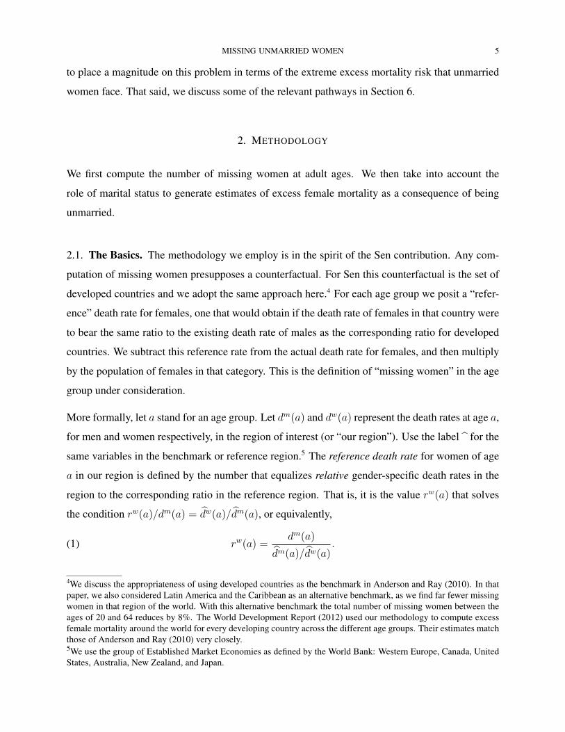
More formally, let a stand for an age group. Let dm(a) and dw(a) represent the death rates at age a,

for men and women respectively, in the region of interest (or “our region”). Use the label for the

same variables in the benchmark or reference region.5 The reference death rate for women of age

a in our region is defined by the number that equalizes relative gender-specific death rates in the

region to the corresponding ratio in the reference region. That is, it is the value rw(a) that solves

the condition rw(a)/dm(a) = dw(a)/dm(a), or equivalently,

(1) rw(a) =dm(a)

dm(a)/dw(a).

4We discuss the appropriateness of using developed countries as the benchmark in Anderson and Ray (2010). In thatpaper, we also considered Latin America and the Caribbean as an alternative benchmark, as we find far fewer missingwomen in that region of the world. With this alternative benchmark the total number of missing women between theages of 20 and 64 reduces by 8%. The World Development Report (2012) used our methodology to compute excessfemale mortality around the world for every developing country across the different age groups. Their estimates matchthose of Anderson and Ray (2010) very closely.5We use the group of Established Market Economies as defined by the World Bank: Western Europe, Canada, UnitedStates, Australia, New Zealand, and Japan.


This methodology turns a blind eye to the prevailing level of the death rates in our region, thereby

implicitly acknowledging that the region can be relatively poor and so prone to greater overall

mortality. But it demands that whatever that higher death rate might be, the ratio of women dying

relative to men should be no different compared to that in the reference region.6 And if we accept

that, then the number of age-specific extra female deaths, or “missing women,” in our region in

a given year would be equal to the difference between the actual and reference death rates for

women, weighted by the number of women in that age group:

(2) EFM(a) = [dw(a)− rw(a)]πw(a),

where πw(a) is the starting population of women of age a. Notice that while the reference death

rate is not affected by the average mortality rate, this estimate is: the absolute numbers of missing

women would increase with higher average mortality, ceteris paribus.

Anderson and Ray (2010) discuss the interpretation of (2) in some detail. In particular, excess

female mortality might arise from a number of causes, and only some of these are explicitly inter-

pretable as discrimination against women, the most obvious examples being excess female mor-

tality at the pre-natal stage, or at birth or in infancy. Other factors, such as excess female mortality

from cardiovascular disease or HIV/AIDS, need a more nuanced interpretation. We do not revisit

these issues here but refer the interested reader to our earlier paper.

2.2. Marriage Rates and Elevation Ratios. We describe a strategy for identifying excess female

deaths, if any, due to unmarriage. This is a subtle problem. Typically, both unmarried men and

women have higher death rates, correcting for age. To the extent that creates larger numbers of

deaths all around, it also creates a larger number of excess female deaths as well. But there is a

second factor at work, which is the comparative extent by which the death rates for women are

raised. To be sure, these ratios are elevated for both our region as well as the reference region. For

our purposes we will need to compare two sets of ratios. All this will be made clearer with a bit

more notation and formalism.

6We are, of course, aware that any such “adjustment method” can be criticized; see Anderson and Ray (2010) for adiscussion of this point. But keeping the ratio constant has a strong intuitive appeal. Besides, this is the approachpredominantly taken in the literature since the work of Sen.


There is also the question of finer categories of unmarriage: widowed, divorced, or never-married.

Data limitations force us to lump these subcategories together. We postpone further discussion to

Section 3.3.

Let σm(a) and σw(a) be the incidence of unmarried men and women respectively in age group a.

For instance, if σm(a) = 0.1, then 10% of all men in age group a are unmarried; and 90% are

married. Denote by em(a) and ew(a) the elevation factors for males and females respectively; that

is, the relative rise in the death rates conditional on lack of marriage. For instance, if ew(a) = 1.1,

then unmarried women in age group a are 10% more likely to die, compared to married women in

that age group.

2.3. Excess Female Mortality by Marital Category. Our focus is on marriage — or the lack

thereof — and to get at this it will be useful to proceed in a couple of steps. Begin by carrying

out the same exercise leading up to (1), but starting with married individuals. That is, let δw(a)

and δm(a) be the death rates for married females and males, respectively. Use the label to denote

these same variables for the benchmark or reference region. We can now generate a “reference”

death rate for married women of age a in our region of interest by

(3) ρw(a) =δm(a)

δm(a)/δw(a),

and we are then in a position to define excess female mortality with marriage benchmarks (EFM0)

at age a by

(4) EFM0(a) = [δw(a)− ρw(a)]πw(a),

where πw(a) is, as before, the entire population of females of age a. Note that we are multiplying

by the full female population, so this is not an estimate of how many women are missing among

the married. It is an estimate of missing women in the entire population under the presumption

that the death rates for married individuals apply to everyone. So, for instance, if the married and

unmarried death rates were all the same for women and men, then EFM(a) = EFM0(a). But if

there is elevation, then EFM(a) > EFM0(a). We are interested in the empirical magnitude of this

difference.


Let us make the connection clearer by converting the values on the right-hand side of (4) into the

aggregated rates that we have in (2). Recalling the elevation factors and marriage incidence rates

already defined, we see that

(5) di(a) =[σi(a)ei(a) + (1− σi(a))

]δi(a) ≡ ci(a)δi(a),

for i = m,w, where cm(a) and cw(a) are “corrections” that are generated by the elevation factors,

and by the proportions of married males and females.

An increase in the elevation factor ei(a) raises ci(a). Moreover, given some ei(a) > 1, a greater

incidence of unmarriage will also increase ci(a), as there is a shift away from the lower death rate

category. In short, larger values of ci point to higher death rates in the unmarried category, and

conditional on that, is correlated with a lower incidence of marriage.

Use the labelto denote these same variables for the benchmark or reference region. Invoking (5)

for both regions and both genders, we have

ρw(a) =δm(a)

δm(a)/δw(a)

=dm(a)

dm(a)/dw(a)

1/cm(a)

cw(a)/cm(a)

= rw(a)1/cm(a)

cw(a)/cm(a),(6)

where rw(a) is the unbiased death rate for all women in our region at age a, defined earlier in (1).

Using (5) and (6) in (4), we must conclude that

EFM0(a) = [δw(a)− ρw(a)]πw(a)

=

[dw(a)

cw(a)− rw(a)

1/cm(a)

cw(a)/cm(a)

]πw(a)

=

[dw(a)− rw(a)

cw(a)/cm(a)

cw(a)/cm(a)

]πw(a)

cw(a)

≡ [dw(a)− θ(a)rw(a)]πw(a)

cw(a),(7)

where

θ(a) =cw(a)/cm(a)

cw(a)/cm(a)


can be viewed as the relative elevation at age a in the region, compared to the reference region.

Recall that ci(a) is larger the greater the elevation factors and the smaller the incidence of marriage.

Moreover, the larger these differences in our region, compared to the reference region, the larger

is the value of θ(a).

The gap between EFM and EFM0 can be viewed as the additional number of missing women due

to unmarriage (and the consequently higher death rates). Call this gap EFM1, then

EFM1(a) ≡ EFM(a)− EFM0(a)

= [dw(a)− rw(a)] πw(a)− [dw(a)− θ(a)rw(a)]πw(a)

cw(a)

=

[1− 1

cw(a)

]EFM(a) + [θ(a)− 1]rw(a)

πw(a)

cw(a).(8)

There are two components in this equation. The first is what one might call the marriage incidence

effect, and is given by the term [1 − (1/cw(a))]EFM(a). Lower marriage — typically because of

widow(er)hood — increases death rates for both men and women, and makes cw(a) larger than 1.

This elevation is more accentuated the higher the rate of unmarriage. Even if the relative death rates

for women change exactly the same way for both the reference region and the region of interest (so

that θ(a) = 1), this will still increase the total number of missing women relative to the marriage

benchmark. After all, the absolute gap between the death rate and its reference counterpart will

have widened.

The second component is what might be termed the skewed elevation ratio effect, and is given by

the term [θ(a)− 1]rw(a)(πw(a)/cw(a)) in (8). If female death rates in our region climb with lack

of marriage at a rate that exceeds the benchmark rate of the reference region, then this increases the

value of θ(a) and contributes to missing women. (Even though it might increase the denominator

cw(a) as well, the net effect is positive.7) We will need to be guided by the data on this matter, but

there are reasons to believe that the female correction factor does indeed bear a higher ratio to its

male counterpart in the region of interest, relative to the reference region. First, if there is a large

gap between male and female age at marriage in the region of interest, adult women will tend to

be widowed more often, so that the rate of unmarriage will be higher, especially in the middle-age

category. Second, if the traditional discrimination against women is reflected to a proportional

7After all, θ(a)−1cw(a) equals 1/cm(a)

cw(a)/cm(a) −1

cw(a) .


degree in widowhood, the relative elevation ratio ew(a)/em(a) will tend to be higher in the region

of interest. Both factors work in the same direction: they raise the female correction factor relative

to the male factor in the region of interest.

It is also worth reiterating that the correction term c is generated from two sources: one is the

ratio of elevation factors, and the other is the incidence of unmarriage. Of course, the latter has

no meaning in the absence of the former: if e were 1, then the incidence of unmarriage would be

irrelevant. On the other hand, if e > 1 (and we shall see that this is indeed the case), then a lower

marriage rate raises the correction term. In an effort to disentangle the “pure” effect of the elevation

ratio from the additional impact of marriage incidence, we can decompose each component of (8)

into two parts. We can do so by first shutting down the differential incidence of marriage altogether,

by simply using the rates of marriage that prevail in the reference region. That is, we can define

pseudo-correction factors for the region of interest by

cie(a) ≡ σi(a)ei(a) + (1− σi(a))

for i = m,w, and a pseudo relative elevation, given by

θe(a) ≡cwe (a)/c

me (a)

cw(a)/cm(a).

With these in hand, we can define a new measure of missing women from non-marriage, call it

EFM1e, which allows for the elevation but not the different rates of marriage across the two regions.

It is given by the following analogue of (8) for each age group a:

(9) EFM1e(a) ≡

[1− 1

cwe (a)

]EFM(a) + [θe(a)− 1]rw(a)

πw(a)

cwe (a).

It also has two components, of course, just as EFM1e did. The remaining term is

EFM1(a)− EFM1e(a)

as a matter of accounting, and can be tentatively interpreted as the additional number of missing

women due to changes in marriage incidence alone. This term may be positive or negative. If

unmarriage rates are high in the region of interest, say due to widowhood, this term will also make

a positive contribution.


Just how large EFM1(a) and EFM1e(a) are is in practice an empirical question, and the goal of this

paper is to provide both estimates.

3. DATA

In our computations of EFM1(a) and EFM1e(a), we focus on the ages 20 to 64.8 Our regions of

interest are India, China, South Asia (excluding India), Southeast Asia, West Asia, East Africa,

West Africa, Middle Africa, South Africa, and North Africa. That is, we focus on regions where

there is excess female mortality to begin with: in other parts of the developing world, such as East

Asia (excluding China), Central Asia, and Latin America and the Caribbean we find no excess

female mortality at adult ages.

To compute EFM1(a) and EFM1e(a), we require data to determine dw(a), dm(a), σw(a), ew(a),

σm(a), em(a) and πw(a) for our regions of interest and for our reference region. Estimates on

mortality rates by age and gender (dw(a) and dm(a)) for age groupings of five years, as well as

female population by age (πw(a)) are readily available for all countries from the United Nations

Department of Economic and Social Affairs.9 Accurate mortality data, by age and gender, for many

developing countries is typically very difficult to obtain. Relying primarily on micro-level surveys

and censuses, to the best of our knowledge, these are the best country-level estimates available. We

discuss issues surrounding the quality of this mortality data , particularly for developing countries,

further in the Appendix.

Estimates of marital status by age group (σw(a) and σm(a)) are also available for all countries

from the U.N. World Marriage Data 2012.10 For all of our variables we chose the data from the

year 2000 or a year as close as possible to 2000.

Mortality rates by age, gender, and marital status (needed to compute ew(a) and em(a)) are more

difficult to obtain as this information is typically not collected in any regular way by national8Marital status data is also available for the age group 15–19 but the percentage of unmarried individuals is too smallfor developed countries for reliable analysis.9For the mortality data, see http://esa.un.org/unpd/wpp/Excel-Data/mortality.htm. For the datasources and methods used to derive the estimates for mortality rates by age and gender across the different countriesrefer to http://esa.un.org/unpd/wpp/Excel-Data/data-sources.htm. Population data come fromU.N. World Population Prospects: The 2012 Revision.10Refer to: http://www.un.org/esa/population/publications/WMD2012/MainFrame.html.The major sources of data on marital status presented in World Marriage Data 2012 are censuses, sample surveys andnational estimates based on population register data or an estimation methods using census data.


statistical agencies. The U.N. Demographic Yearbook 2003 reports this information for all of these

variables for several countries between 1994–2003. We again select the data from the year 2000 or

the closest to that year as possible, and for as many countries as we can. That gives us enough data

to compute ew(a) and em(a) for all developed countries. This information, however, is far rarer

for developing countries. For our regions of interest, we have this data for four countries in Africa

(Egypt, Mauritius, Reunion, and Tunisia), and ten countries in Asia (Hong Kong, Macao, Japan,

Kazakhstan, Republic of Korea, Singapore, Qatar, State of Palestine, Georgia, and Azerbaijan).

We use the data to compute various estimates of elevation factors for our regions of interest. For

example, we compute one set of elevation factors for Africa by aggregating across the countries

within this region that we have data for, and likewise for Asia. We will then compute our estimates

of EFM1(a) and EFM1e(a) for our regions of interest under different specifications which vary

by the elevation factors we compute for these regions. We discuss the implications of different

specifications in detail in Section 4. Given the paucity of data, it makes little sense to disaggregate

“unmarriage” any further; on this, see Section 3.3.

Key to the computation of EFM1(a) is the size of θ(a), which is the female-male ratio of correction

factors at age a in our region of interest, relative to the same ratio in the reference region. The

larger the female-male correction factor in our region — influenced positively by both the elevation

ratio and the overall incidence of unmarriage — the larger is the value of θ(a). That is, recalling

that a typical correction factor c(a) (dropping superscripts) is given by σ(a)e(a) + (1 − σ(a)), it

follows that θ(a) is increasing in ew(a)/em(a) relative to the same ratio in our reference region,

ew(a)/em(a). It is also increasing in σw(a)/σm(a) relative to its reference value σw(a)/σm(a).

We now build these ratios from the data.

3.1. Marital Status by Age. We first consider σm(a) and σw(a), the incidence of unmarried men

and women respectively in age group a, in both our regions of interest and in our reference region.

What is most relevant for the determination of EFM1(a) is the size of the ratio σw(a)/σm(a)

relative to the same ratio in our reference region, σw(a)/σm(a). Figure 1 plots this relative ratio

for our regions of interest, and for developed countries, our reference region. We see that the ratio

σw(a)/σm(a) for less developed regions is higher than for developed regions for ages older than

35. The only exception is China where this ratio is lower than for developed countries.


0"

1"

2"

3"

4"

5"

6"

17" 22" 27" 32" 37" 42" 47" 52" 57" 62"

Age$

India"

Developed"

China"

South"Asia"

Southeast"Asia"

West"Asia"

σ w

σm

(a) Asia

0"

1"

2"

3"

4"

5"

6"

7"

17" 22" 27" 32" 37" 42" 47" 52" 57" 62"

Age$

Developed"

East"Africa"

Middle"Africa"

North"Africa"

Southern"Africa"

West"Africa"

σ w

σm

(b) Africa

Figure 1. THE RATIO σw(a)/σm(a) FOR DIFFERENT REGIONS AND AGES.

Unmarried individuals could be widowed, divorced or single. The second and third subcate-

gories are largely symmetric across men and women, so the high values of σw(a)/σm(a) are

primarily driven by the proportions of widows (relative to widowers) in all regions. The fact

that σw(a)/σm(a) is lower in developed countries relative to developing is a sign of the fact that

this imbalance is heightened in developing countries, at all age groups.11 For more discussion, see

Section 3.3.

3.2. Elevation. The second key component in our computation of EFM1(a) are the elevation fac-

tors em(a) and ew(a), which reflect the relative mortality rates of unmarried and married individu-

als by gender and age.

As discussed, we construct three main sets of elevation factors. The first is for our reference region,

which is a population-weighted average across all developed countries. We then construct average

elevation factors for two areas of the developing world under consideration: Africa (using the

available data from Egypt, Mauritius, Reunion, and Tunisia) and Asia (using data from Hong Kong,

Macao, Japan, Kazakhstan, Republic of Korea, Singapore, Qatar, State of Palestine, Georgia, and

Azerbaijan). We discuss the implications of relying on these samples of countries to construct the

elevation factors for our different regions of interest in Section 4.

11In addition, relative to developed countries, divorce is far less common in developing countries. In India and the restof South Asia, the incidence of divorce is less than 1% in all age groups for men and women. In the rest of Asia it isat most 2%. In Africa, divorce is somewhat more common at around 5%.


0"

0.5"

1"

1.5"

2"

2.5"

3"

3.5"

4"

17" 22" 27" 32" 37" 42" 47" 52" 57" 62"Age$

Asia"

Africa"

Developed"

we

(a) Females

0"

0.5"

1"

1.5"

2"

2.5"

3"

3.5"

4"

4.5"

5"

17" 22" 27" 32" 37" 42" 47" 52" 57" 62"Age$

Asia"

Africa"

Developed"

me

(b) Males

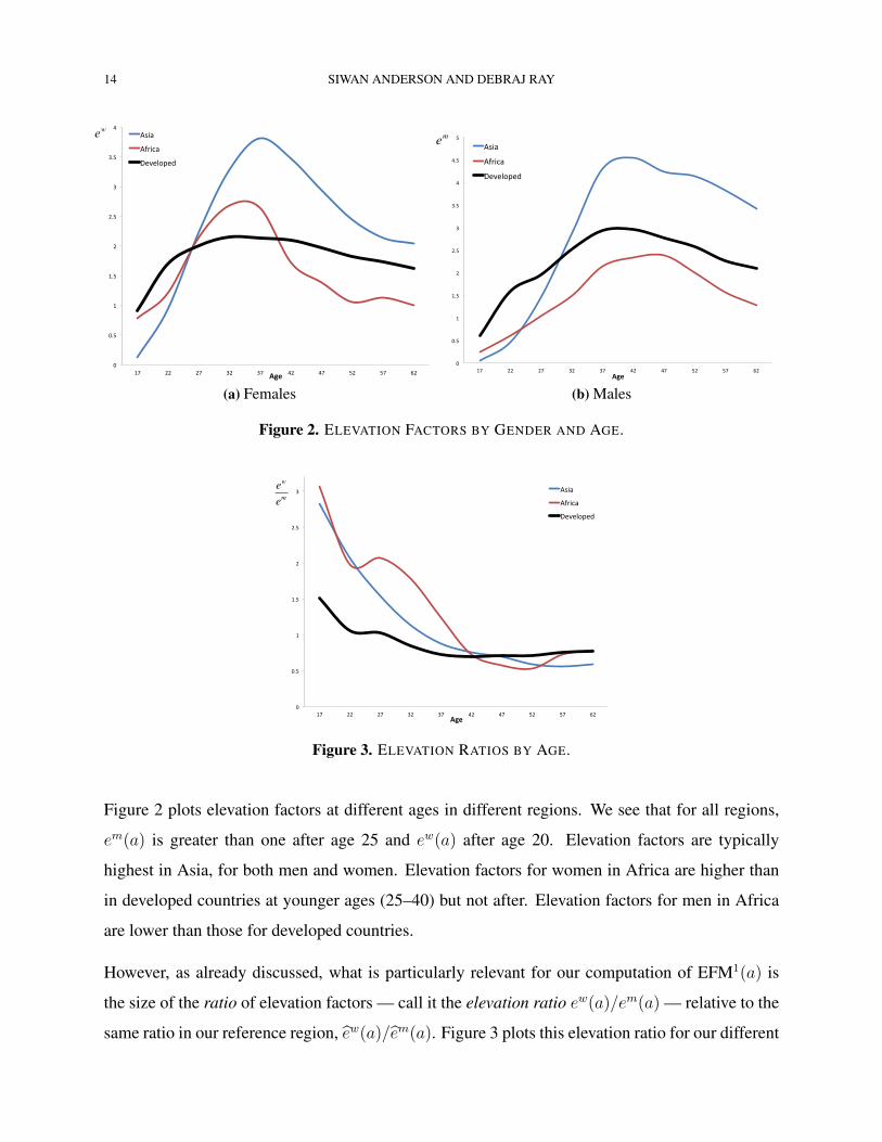
Figure 2. ELEVATION FACTORS BY GENDER AND AGE.

0"

0.5"

1"

1.5"

2"

2.5"

3"

17" 22" 27" 32" 37" 42" 47" 52" 57" 62"Age$

Asia"

Africa"

Developed"

ew

em

Figure 3. ELEVATION RATIOS BY AGE.

Figure 2 plots elevation factors at different ages in different regions. We see that for all regions,

em(a) is greater than one after age 25 and ew(a) after age 20. Elevation factors are typically

highest in Asia, for both men and women. Elevation factors for women in Africa are higher than

in developed countries at younger ages (25–40) but not after. Elevation factors for men in Africa

are lower than those for developed countries.

However, as already discussed, what is particularly relevant for our computation of EFM1(a) is

the size of the ratio of elevation factors — call it the elevation ratio ew(a)/em(a) — relative to the

same ratio in our reference region, ew(a)/em(a). Figure 3 plots this elevation ratio for our different


0"

0.1"

0.2"

0.3"

0.4"

0.5"

0.6"

0.7"

0.8"

0.9"

1"

17" 22" 27" 32" 37" 42" 47" 52" 57" 62"

Age$

Developed"China"India"Africa"

(a) Single/Unmarried: Males

0"

0.1"

0.2"

0.3"

0.4"

0.5"

0.6"

0.7"

0.8"

0.9"

1"

17" 22" 27" 32" 37" 42" 47" 52" 57" 62"

Age$

Developed"

China"

India"

Africa"

(b) Single/Unmarried: Females

0"

0.1"

0.2"

0.3"

0.4"

0.5"

0.6"

0.7"

0.8"

17" 22" 27" 32" 37" 42" 47" 52" 57" 62"Age$

Developed"China"India"Africa"

(c) Widowed/Unmarried: Males

0

0.1

0.2

0.3

0.4

0.5

0.6

0.7

0.8

0.9

1

17 22 27 32 37 42 47 52 57 62

Age

Developed

China

India

Africa

(d) Widowed/Unmarried: Females

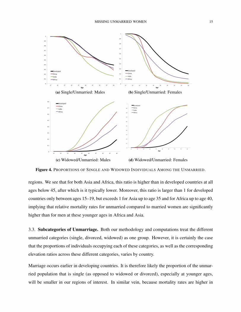
Figure 4. PROPORTIONS OF SINGLE AND WIDOWED INDIVIDUALS AMONG THE UNMARRIED.

regions. We see that for both Asia and Africa, this ratio is higher than in developed countries at all

ages below 45, after which is it typically lower. Moreover, this ratio is larger than 1 for developed

countries only between ages 15–19, but exceeds 1 for Asia up to age 35 and for Africa up to age 40,

implying that relative mortality rates for unmarried compared to married women are significantly

higher than for men at these younger ages in Africa and Asia.

3.3. Subcategories of Unmarriage. Both our methodology and computations treat the different

unmarried categories (single, divorced, widowed) as one group. However, it is certainly the case

that the proportions of individuals occupying each of these categories, as well as the corresponding

elevation ratios across these different categories, varies by country.

Marriage occurs earlier in developing countries. It is therefore likely the proportion of the unmar-

ried population that is single (as opposed to widowed or divorced), especially at younger ages,

will be smaller in our regions of interest. In similar vein, because mortality rates are higher in


0"

0.2"

0.4"

0.6"

0.8"

1"

1.2"

1.4"

1.6"

17" 22" 27" 32" 37" 42" 47" 52" 57" 62"Age$

Single"

Widow"

Divorce"

m

w

ee

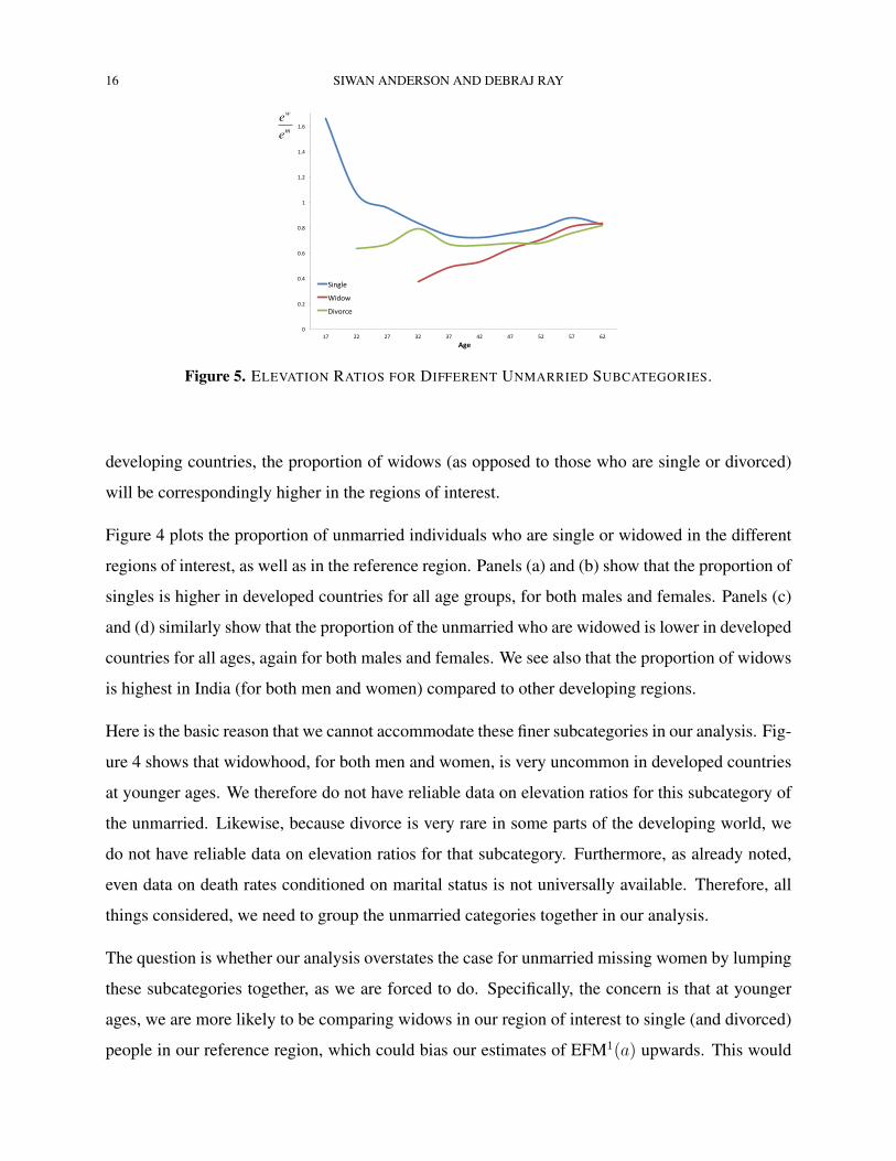
Figure 5. ELEVATION RATIOS FOR DIFFERENT UNMARRIED SUBCATEGORIES.

developing countries, the proportion of widows (as opposed to those who are single or divorced)

will be correspondingly higher in the regions of interest.

Figure 4 plots the proportion of unmarried individuals who are single or widowed in the different

regions of interest, as well as in the reference region. Panels (a) and (b) show that the proportion of

singles is higher in developed countries for all age groups, for both males and females. Panels (c)

and (d) similarly show that the proportion of the unmarried who are widowed is lower in developed

countries for all ages, again for both males and females. We see also that the proportion of widows

is highest in India (for both men and women) compared to other developing regions.

Here is the basic reason that we cannot accommodate these finer subcategories in our analysis. Fig-

ure 4 shows that widowhood, for both men and women, is very uncommon in developed countries

at younger ages. We therefore do not have reliable data on elevation ratios for this subcategory of

the unmarried. Likewise, because divorce is very rare in some parts of the developing world, we

do not have reliable data on elevation ratios for that subcategory. Furthermore, as already noted,

even data on death rates conditioned on marital status is not universally available. Therefore, all

things considered, we need to group the unmarried categories together in our analysis.

The question is whether our analysis overstates the case for unmarried missing women by lumping

these subcategories together, as we are forced to do. Specifically, the concern is that at younger

ages, we are more likely to be comparing widows in our region of interest to single (and divorced)

people in our reference region, which could bias our estimates of EFM1(a) upwards. This would


(1) (2) (3)Age EFM1(a) EFM1

e(a) EFM1(a) EFM1e(a) EFM1(a) EFM1

e(a)

20-24 16 28 16 27 23 4725-29 7 35 7 36 10 4230-34 13 25 13 24 14 2835-39 21 13 21 12 19 940-44 24 4 25 5 19 -545-49 25 1 26 1 20 -1050-54 25 -4 26 -4 21 -1455-59 18 -7 20 -5 14 -1460-64 34 1 41 6 29 -7

Total 184 194 170% Unmarr. Females 0.48 0.51 0.45

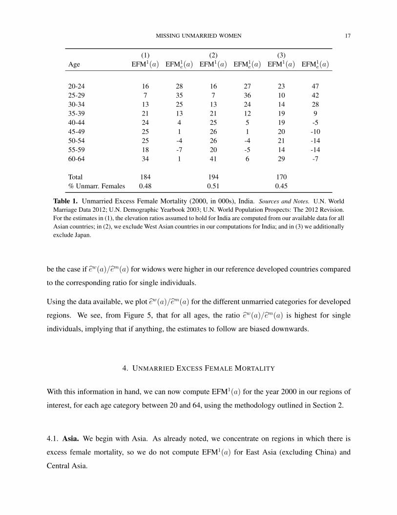
Table 1. Unmarried Excess Female Mortality (2000, in 000s), India. Sources and Notes. U.N. WorldMarriage Data 2012; U.N. Demographic Yearbook 2003; U.N. World Population Prospects: The 2012 Revision.For the estimates in (1), the elevation ratios assumed to hold for India are computed from our available data for allAsian countries; in (2), we exclude West Asian countries in our computations for India; and in (3) we additionallyexclude Japan.

be the case if ew(a)/em(a) for widows were higher in our reference developed countries compared

to the corresponding ratio for single individuals.

Using the data available, we plot ew(a)/em(a) for the different unmarried categories for developed

regions. We see, from Figure 5, that for all ages, the ratio ew(a)/em(a) is highest for single

individuals, implying that if anything, the estimates to follow are biased downwards.

4. UNMARRIED EXCESS FEMALE MORTALITY

With this information in hand, we can now compute EFM1(a) for the year 2000 in our regions of

interest, for each age category between 20 and 64, using the methodology outlined in Section 2.

4.1. Asia. We begin with Asia. As already noted, we concentrate on regions in which there is

excess female mortality, so we do not compute EFM1(a) for East Asia (excluding China) and

Central Asia.


0"

0.2"

0.4"

0.6"

0.8"

1"

22" 27" 32" 37" 42" 47" 52" 57" 62"Age$$

India"

China"

South"Asia"

Southeast"Asia"

West"Asia"

Figure 6. PROPORTION OF EFM1(a) ATTRIBUTABLE TO THE CORRECTION FACTOR EFFECT INASIA.

The first column of Table 1 lists the numbers of missing unmarried women in each age sub-category

in the overall range 20–65, for India. In all see that there are approximately 180,000 missing

women due to unmarriage in India in the year 2000. A significant proportion of this number (44%)

are in the reproductive age category 20–45.

In this first set of estimates listed in Column 1, the assumed elevation ratios ew(a)/em(a) for India

are computed from our available data for all Asian countries. In the next set of estimates (Column

2), we exclude West Asian countries in our computations of the elevation ratio. In the final set of

estimations (Column 3), we also exclude Japan so that the sample of countries used to compute

the elevation ratios for India are only from East Asia (excluding China and Japan) and Central

Asia. (In both these regions we find no excess female mortality for ages older than 15.) We see

that our estimates of EFM1(a) do not change significantly across the different approximations.

Given the evidence of discrimination against unmarried women in India and the rest of South Asia

(discussed in the introduction), we would expect that ew(a)/em(a) would most likely be higher

for India and other South Asian countries compared to the rest of Asia, particularly compared to

East Asia (excluding China and Japan) and Central Asia. If this is the case, then our estimates of

EFM1(a) for India are, if anything, biased downwards.

In Section 2.3, we demonstrated how EFM1(a) could be divided into two components, the marriage

incidence effect and the skewed elevation ratio effect. In Figure 6, we plot the proportion of


EFM1(a) which can be attributed to the skewed elevation ratio effect for different Asian regions,

including India, by age. We see that EFM1(a) is primarily composed of this factor for all ages,

with a slight decrease with age. This demonstrates the importance of a high value of

θ(a) =cw(a)/cm(a)

cw(a)/cm(a)

in determining excess female mortality from the absence of marriage in Asia in general, and India

in particular. That is, the female correction factor does indeed bear a higher ratio to its male

counterpart in India, relative to the reference region. As the discussion to follow will show, it is

not just the elevation ratios but also the high rates of widowhood in India (after age 40) that drive

the large values of θ(a).

Recall from Section 2.3 that the correction factor, which drives excess female mortality from the

absence of marriage, is generated from two sources. One is that the elevation ratios ew(a)/em(a)

are larger in our country of interest, compared to those in our reference region. The other is that the

incidence of marriage is different across the two regions. We now attempt to disentangle these two

effects. For each of the estimates in Columns 1–3 in Table 1, we report corresponding estimates

of EFM1e(a) for each age group. Recall from Section 2.3 that this particular estimate of missing

unmarried women allows for different elevation ratios but not different rates of marriage across

the two regions. That is, we assume the rate of unmarriage by age group is identical across India

and our reference region. We see that these estimates are largest in the younger age categories

(ages 20 to 40). This implies that the excess unmarried female mortality at these younger ages,

primarily follows from the fact that the elevation ratio for Asia is high relative to the same ratio

in our reference region. But above the age of 40, a different phenomenon takes over. Notice

that EFM1(a)− EFM1e(a) is a measure of missing women due to changes in marriage incidence

alone. These numbers are large and positive for ages above 40. So in other words, it is the large

incidence of widowhood in India, at ages above 40, which is primarily driving the excess mortality

for unmarried women at these older ages.

Table 2 turns to South Asia, excluding India. In this region, we see that there are more than

60,000 missing unmarried women each year. As a percentage of the total population of unmarried

females, there is a lower number of missing women due to unmarriage in South Asia compared

to India. But the remaining pattern is roughly similar to that in India. Again, approximately 45%


(1) (2) (3)Age EFM1(a) EFM1


e(a)

20-24 7 10 7 10 10 1825-29 3 9 3 9 4 1130-34 4 8 4 8 5 935-39 6 6 6 6 6 540-44 7 4 7 4 6 245-49 7 2 7 3 6 050-54 8 1 8 1 7 -155-59 7 0 8 0 7 -160-64 12 2 14 4 12 1


Table 2. Unmarried Excess Female Mortality (2000, in 000s), South Asia excluding India. Sources andNotes. U.N. World Marriage Data 2012; U.N. Demographic Yearbook 2003; U.N. World Population Prospects:The 2012 Revision. For the estimates in (1), the elevation ratios assumed to hold for South Asia are computedfrom our available data for all Asian countries; in (2), we exclude West Asian countries in our computations; andin (3) we additionally exclude Japan.

of the missing unmarried women are of reproductive age. Figure 6 also tells us that as in India,

EFM1(a) for South Asia is primarily composed of the skewed elevation ratio effect at all ages,

with a slight decrease with age. Likewise, our estimates of EFM1e(a) for South Asia show that it

is the high elevation ratios in Asia which drive excess mortality from the absence of marriage at

these younger ages, whereas it is the incidence of widowhood which drives it at the older ages.

Table 3 records 85,000 missing unmarried women each year in Southeast Asia. As a percentage

of the total population of unmarried females, there are fewer missing unmarried women in this

region compared to the countries of South Asia (not counting India). Again, from Figure 6, we see

that EFM1(a) for Southeast Asia is primarily composed of the skewed elevation ratio effect at all

ages, though this component is slightly smaller compared to other regions of Asia. Our estimates

of EFM1e(a) suggest that the patterns of excess unmarried female mortality by age follow similar

patterns across this region and the countries of South Asia, where again high elevation ratios in

Asia drive this excess mortality at the younger ages and the incidence of widowhood drives it at

the older ages.


(1) (2) (3)Age EFM1(a) EFM1


e(a)

20-24 11 17 11 17 17 3025-29 7 11 6 10 8 1330-34 8 8 8 7 9 835-39 10 4 10 4 8 240-44 11 2 11 2 8 -245-49 11 1 11 1 8 -450-54 10 -2 10 -2 8 -655-59 9 -4 9 -4 7 -760-64 11 -2 14 -1 10 -6


Table 3. Unmarried Excess Female Mortality (2000, in 000s), South-East Asia. Sources and Notes. U.N.World Marriage Data 2012; U.N. Demographic Yearbook 2003; U.N. World Population Prospects: The 2012Revision. For the estimates in (1), the elevation ratios assumed to hold for Southeast Asia are computed from ouravailable data for all Asian countries; in (2), we exclude West Asian countries in our computations; and in (3) weadditionally exclude Japan.

Table 4 provides our estimates for China. We see that relative to countries in South and Southeast

Asia, there are very few missing unmarried women in China. The few that are missing are at

the younger adult ages and they are due to the high elevation ratios for Asia that we’ve imputed to

China. There are almost no unmarried missing women in China due to the relatively high incidence

of widowhood (or not being married). The final two columns of Table 4 demonstrate that likewise

there is little excess female mortality due to the absence of marriage in West Asia. From Figure 6,

we see that EFM1(a) for these two regions is almost entirely composed of the elevation ratio effect

component for all ages.

4.2. Africa. We now turn to Africa.

Table 5 shows that there are approximately 255,000 missing unmarried women in Africa in the year

2000. Roughly 47% of these are from East Africa, where as a percentage of the total population

of unmarried women the numbers are also the highest. By contrast, the countries of North Africa

have the lowest levels of excess female mortality from unmarriage.


China (1) China (2) China (3) West AsiaAge EFM1(a) EFM1


e(a) EFM1(a) EFM1e(a)

20-24 12 16 12 17 9 12 3 425-29 5 19 5 19 2 15 1 230-34 6 16 6 15 4 12 2 235-39 7 9 6 9 6 6 2 140-44 5 4 4 5 5 3 2 045-49 3 5 3 5 4 2 1 050-54 0 -1 0 -1 0 -3 1 -155-59 -4 -5 -4 -4 -4 -6 0 -260-64 -3 -2 0 2 -2 -2 -2 -3

Total 31 32 23 9% Unmarr. Females 0.07 0.07 0.05 0.07

Table 4. Unmarried Excess Female Mortality (2000, in 000s), China and West Asia. Sources and Notes.U.N. World Marriage Data 2012; U.N. Demographic Yearbook 2003; U.N. World Population Prospects: The2012 Revision. For the estimates in (1), the elevation ratios assumed to hold for China are computed from ouravailable data for all Asian countries; in (2), we exclude West Asian countries in our computations for China; andin (3) we include only countries from East Asia. In the final two columns we use the elevation ratios from WestAsian countries to obtain corresponding estimates for West Asia.

East Middle Southern West NorthAge EFM1(a) EFM1



e(a)

20-24 12 21 4 8 3 3 14 22 4 425-29 21 40 5 10 8 8 11 25 3 430-34 32 43 6 9 10 9 10 20 3 435-39 30 28 6 6 8 7 9 13 3 340-44 14 6 3 2 4 2 6 3 2 145-49 6 0 2 0 1 0 4 0 2 050-54 2 -2 0 -1 -1 -1 2 -2 1 -155-59 2 0 1 0 0 0 3 0 1 060-64 0 -1 -1 0 0 0 -1 -1 0 -1

Total 119 28 31 58 19% 0.79 0.59 0.46 0.54 0.15

Table 5. Unmarried Excess Female Mortality (2000, in 000s), Africa. Sources and Notes. U.N. WorldMarriage Data 2012; U.N. Demographic Yearbook 2003; U.N. World Population Prospects: The 2012 Revision.

In Figure 7, we plot the proportion of EFM1(a) which is attributable to the skewed elevation ratio

effect for the different African regions by age. We see that, like the regions of Asia, EFM1(a) is

primarily composed of this component for all ages. Compared to Asia, this component is somewhat

smaller in Africa, and unlike in Asia it also increases slightly with age. But overall, Figure 7 is in

accordance with Figure 6 in that they both demonstrate the importance of a high value of θ(a) in


0"

0.2"

0.4"

0.6"

0.8"

1"

22" 27" 32" 37" 42" 47" 52" 57" 62"

Age$

East"Africa"

Middle"Africa"

North"Africa"

Southern"Africa"

West"Africa"

Figure 7. PROPORTION OF EFM1(a) ATTRIBUTABLE TO THE CORRECTION FACTOR EFFECT INAFRICA.

determining excess female mortality from the absence of marriage in Africa as well. That is, the

female correction factor does indeed bear a higher ratio to its male counterpart in Africa, relative

to the reference region.

Almost all of the missing unmarried women in Africa are at the younger ages: 91% of them are

between the ages 20 and 45. From our computations of EFM1e(a) across the regions of Africa, we

see that these are mainly due to the high elevation ratios for Africa relative to the same ratio in our

reference region.

Notice that the elevation ratios assumed for Africa are derived primarily from available data from

North Africa. That, incidentally, is the region in Africa with the least overall excess female adult

mortality. To the extent that the mortality risks that unmarried women face in the other regions of

Africa are higher, our estimates of EFM1(a) for these other regions are likely underestimates.

5. UNMARRIED EXCESS FEMALE MORTALITY AND MISSING WOMEN

We are now in a position to compare our estimates of unmarried excess female mortality, EFM1(a),

to overall estimates of overall excess female mortality, EFM(a). In Table 6, we compute aggregate

measures of both kinds of excess mortality by aggregating age-specific estimates of EFM(a) and

EFM1(a) across different age groups (20 to 64). Comparing these totals enables us to determine

how much of the overall excess female mortality in developing regions can be attributed to not

having a husband.


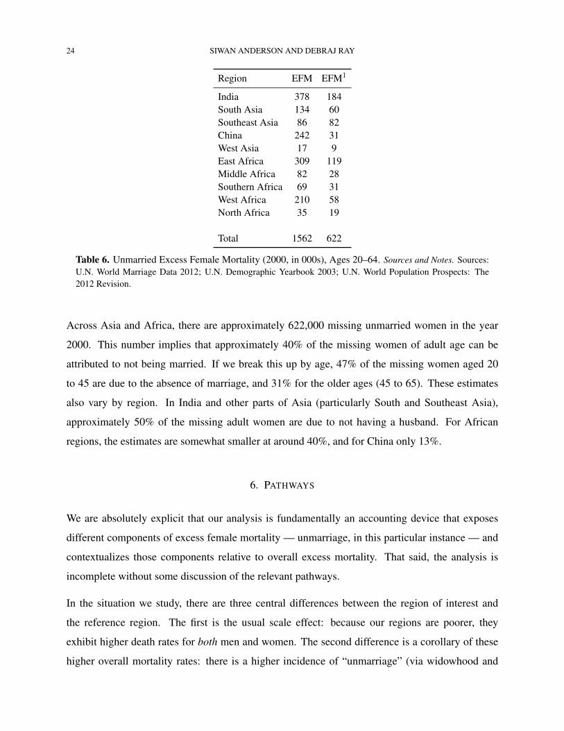
Region EFM EFM1

India 378 184South Asia 134 60Southeast Asia 86 82China 242 31West Asia 17 9East Africa 309 119Middle Africa 82 28Southern Africa 69 31West Africa 210 58North Africa 35 19

Total 1562 622

Table 6. Unmarried Excess Female Mortality (2000, in 000s), Ages 20–64. Sources and Notes. Sources:U.N. World Marriage Data 2012; U.N. Demographic Yearbook 2003; U.N. World Population Prospects: The2012 Revision.

Across Asia and Africa, there are approximately 622,000 missing unmarried women in the year

2000. This number implies that approximately 40% of the missing women of adult age can be

attributed to not being married. If we break this up by age, 47% of the missing women aged 20

to 45 are due to the absence of marriage, and 31% for the older ages (45 to 65). These estimates

also vary by region. In India and other parts of Asia (particularly South and Southeast Asia),

approximately 50% of the missing adult women are due to not having a husband. For African

regions, the estimates are somewhat smaller at around 40%, and for China only 13%.

6. PATHWAYS

We are absolutely explicit that our analysis is fundamentally an accounting device that exposes

different components of excess female mortality — unmarriage, in this particular instance — and

contextualizes those components relative to overall excess mortality. That said, the analysis is

incomplete without some discussion of the relevant pathways.

In the situation we study, there are three central differences between the region of interest and

the reference region. The first is the usual scale effect: because our regions are poorer, they

exhibit higher death rates for both men and women. The second difference is a corollary of these

higher overall mortality rates: there is a higher incidence of “unmarriage” (via widowhood and


widowerhood) in our regions of interest.12 Finally, there is a gender bias, reflected in varying

relative elevation ratios across women and men.

Following standard practice (for an extended discussion, see Anderson and Ray 2010), the scale

effect is not included in our computation of excess unmarried female mortality. Indeed, the entire

exercise presumes that the relative, age-specific death rates in the reference region are the “unbi-

ased” death rates, and it is precisely the departures from those “reference rates” that generate our

estimates. How appropriate is this choice? How do we know that gender-based death rates are not

somehow “naturally” different at different levels of development?

This assumption is well-nigh impossible to test with available data. The best we could do is

presume — at least for a sizable set of countries once poor, or poor countries today — that there

is no gender discrimination, so that the relative rates in those countries are the “natural” relative

rates. In our earlier work (Anderson and Ray 2010) we did use Latin American and Caribbean

countries as an alternative reference group. Our estimates of excess female mortality for the age

group 20–64 decrease by only 8%. So one might presume that the reference regions are not far off

the mark to begin with.

But there is a deeper conceptual reason: the use of any reference group that does not replicate

what we see in developed countries today runs the risk of burying important gender differentials

under the cover of an “alternative benchmark.” For instance, we could be labeling as natural and

non-discriminatory the tendency for females to die relatively more in developing countries. We

see absolutely no reason why this should be the case. In our opinion, it is far more satisfactory

to presume that the “natural” relative death rates are indeed constant with development, and then

to view every departure from that benchmark as prima facie cause for suspicion (though not as

conclusive evidence).

Our focus, then, is on differences in the incidence of marriage as well as in the relative elevation

ratios. As we explain in Section 2.3, our methodology allows us to disentangle these two effects.

As an application, split the age range 20–65 that we consider into two groups. Approximately 30%

of the missing unmarried women are in the older group 45-65. Our computations demonstrate that

12It is true that the incidence of marriage is typically higher in our regions, but this is outweighed by the highermortality rates.


excess female mortality amongst this older unmarried group is driven mainly by a high relative

incidence of widowhood in the regions of interest. It may well be that this marriage incidence ef-

fect is not linked directly to gender discrimination, and is just the outcome of age/gender mortality

correlations with development. Further research is needed to identify exactly the sources generat-

ing the significant excess female mortality from the absence of marriage amongst older women in

parts of Asia and Africa.

The remaining 70% of the missing unmarried women are of reproductive age (between 20 and 45

years old). We have demonstrated that it is the skewed elevation ratio effect that that drives excess

female mortality at these younger ages. Younger unmarried women are missing not because their

death rates are elevated — that is true of the reference region as well —but because the elevation

factor for women (compared to that for men) is relatively high in the parts of Asia and Africa

we’ve studied. This is plausibly due to limited access to resources and health care for women in

this very socially marginalized group.

That said, we want to be extremely cautious in interpreting our results as providing direct evidence

of discrimination. We do not want to assert that our numbers — large though they might be — fully

represent overt (or even implicit) discrimination against unmarried women. In general, there will

be an entire complex of social, behavioural, and economic pathways that will need to be invoked.

Our objective in this paper is simply to flag unmarriage as a factor in determining excess female

mortality at older ages in a unified and comparable way across developing countries. The numbers

are striking: in each year, over 620,000 unmarried women are missing.

We cannot, however, prove a causal link between marriage and excess unmarried female mortal-

ity. In the literature examining the relationship between marital status and mortality in developed

countries, a long-standing debate attempts to disentangle the role of “marriage protection” versus

“marital selection” in explaining the observed differences (Goldman 1993). Much of that literature

focuses on the role of “marriage protection”, i.e., the social, psychological, economic, and envi-

ronmental benefits associated with having a spouse, and that help to prevent premature mortality.

A competing explanation is the role of “marital selection”: that healthier individuals (and those

with more stable behavioral traits) are more likely to marry.


Since a randomly controlled experiment is impossible to conduct to identify the relative impor-

tance of these two explanations, researchers have typically turned to large-scale individual-level

longitudinal data to establish a causal role from marriage to better health outcomes, controlling

for observables most likely linked to selection into marriage. Rendall et. al. (2011) claim that

these more recent analyses have led to a stronger case for the “marriage protection” hypothesis.

Moreover, as there does not appear to be significant differences in mortality rates for the differ-

ent categories of “unmarriage” (never married, divorced/separated, and widowed) it is difficult to

argue that the particular traits systematically determining worse health outcomes could simultane-

ously explain selection into these different states of “unmarriage”. Nonetheless, we cannot rule

out the possibility of selection effects in explaining some of the excess unmarried female mortality

that we find for developing countries. It is not just the binary consideration that healthy people

tend to marry, unhealthy people don’t, but the plausibly positive assortative marriage matching

based on health. With such matching, less healthy individuals are more likely to be widows (or

widowers) due to the premature death of their likewise unhealthy spouse. The skewed elevation

ratio effect would then require that the marital sorting on health status in developing countries is

more pronounced relative to the corresponding sorting in developed countries. Moreover, such an

explanation would further require that this sorting pattern is more prevalent in India (and other

parts of South Asia) compared to Africa and China.

7. CONCLUSIONS

It is well known that the absence of marriage can pose significant risks, and that such risk can and

does manifest itself in higher mortality rate for the unmarried. In principle, this is true of both men

and women. There is a more subtle perception that the elevation of risk is higher for women then

for men, and that this relative elevation is particularly acute for developing countries. This is the

starting point of our paper, which attempts to establish the magnitude of this problem and situate it

in a larger context: the phenomenon of “missing women” or excess female mortality in developing

regions.

The numbers we put on this phenomenon are quite remarkable. All told, there are approximately

1.5 million missing women between the ages of 20–64, each year. We find that more than 40% of

these missing women of adult age — over 620,000 of them — can be attributed to “unmarriage,”


which underlines the fundamental relevance and importance of this issue. This percentage is as

high as 55% in India and other regions of South Asia and 45% in Africa. Both these developing

regions are characterized by high excess female adult mortality and a very low social standing

for unmarried women. Further research is needed to identify exactly the sources generating the

significant excess female mortality for this very marginalized group of women.

REFERENCES

Anderson, Siwan and Debraj Ray (2010) ”Missing Women: Age and Disease,” Review of Eco-

nomic Studies 77(4), 1262–1300.

Anderson, Siwan and Debraj Ray (2012) ”The Age Distribution of Missing Women in India,”

Economic and Political Weekly 47, No. 47-48, 87–95.

Chen, Marty and Jean Dreze (1992) ”Widows and Health in Rural North India,” Economic and

Political Weekly 27, No. 43/44, WS81–WS92.

Farr, William (1858), “The Influence of Marriage on the Mortality of the French People,” in Trans-

actions of the National Association for the Promotion of Social Science, edited by G.W. Hastings.

London: John W. Parker. p. 504–13.

Goldman, Noreen (1993), “Marriage Selection and Mortality Patterns: Inferences and Fallacies,”

Demography 30, 189–208.

Jensen, Robert T. (2005) ”Caste, Culture, and the Status and Well-Being of Widows in India,” in

Analyses in the Economics of Aging, David A. Wise (editor), University of Chicago Press, 357–

373.

Johnson, N. J., E. Backlund, P.D. Sorlie, and C.A. Loveless (2000) ”Marital Status and Mortality:

The National Longitudinal Mortality Study,” Annals of Epidemiology 10(4), 224–238.

Liu, Hui and David Johnson (2009), “Till Death Do Us Part: Marital Status and U.S. Mortality

Trends, 1986–2000,” Journal of Marriage and Family 71, 1158–1173.

Miguel, Edward (2005) ”Poverty and Witch Killing,” Review of Economic Studies 72(4), 1153–

1172.


Murphy, Michael, Grundy, Emily and Stamatis Kalogirou (2007), “The Increase in Marital Status

Differences in Mortality up to the Oldest Age in Seven European Countries, 1990–99,” Population

Studies 61, 287–298.

Murray, C. J. L., Ferguson, B. D., Lopez, A. D., Guillot, M., Salomon, J. A. and O. Ahmad (2003),

“Modified Logit Life Table System: Principles, Empirical Validation and Application,” Population

Studies 57, 165–182.

Nagata, C, N. Takatsuka, and H. Shimizu (2003) ”The Impact of Changes in Marital Status on the

Mortality of Elderly Japanese,” Annals of Epidemiology 13(4), 218–222.

Oppong, Christine (2006) ”Familial Roles and Social Transformations: Older Men and Women in

Sub-Saharan Africa,” Research on Aging 28(6), 654–668.

Rahman, Omar, Andrew Foster, and Jane Menken (1992) ”Older Widow Mortality in Rural Bangladesh,”

Social Science and Medicine, 34(1), 89-96.

Rendall, Michael S., Weden, Margaret M., Favreault, Melissa M., and Hilary Waldron (2011), “The

Protective Effect of Marriage for Survival: A Review and Update,” Demography 48, 481–506.

Robards, Maria Evandroua, Falkinghama, Jane and Athina Vlachantonia (2012), “Marital Status,

Health and Mortality,” Maturitas 73, 295–299.

Sen, Amartya (1990) ”More than 100 Million Women are Missing,” The New York Review of

Books, 37(20), 20 December.

Sen, Amartya (1992) ”Missing Women,” British Medical Journal 304, March, 587–88.

Shor, Eran, Roelfs, David J., Bugyi, Paul, and Joseph E. Schwartz (2012), “Meta-Analysis of Mar-

ital Dissolution and Mortality: Reevaluating the Intersection of Gender and Age,” Social Science

and Medicine 75, 46–59.

Sossou, Marie-Antoinette (2002) ”Widowhood Practices in West Africa: The Silent Victims,” In-

ternational Journal of Social Welfare 11, 201–209.

Subramanian, S.V., Felix Elwert, and Nicholas Christakis (2008) ”Widowhood and Mortality

among the Elderly: The Modifying role of Neighborhood Concentration of Widowed Individu-

als,” Social Science and Medicine 66, 873–884.


van de Walle, Dominique (2011) “Lasting Welfare Effects of Widowhood in Mali,” World Bank

Policy Research Working Paper 5734.

World Bank (2012), Gender Equality and Development, World Development Report.

Zheng, Hui and Patricia A. Thomas (2013), “Marital Status, Self-Rated Health, and Mortality:

Overestimation of Health or Diminishing Protection of Marriage?” Journal of Health and Social

Behavior 54, 128–143.

APPENDIX: DATA SOURCES

For this paper we rely on mortality data compiled by The Population Division of the United Nations

(UN), who provide the most comprehensive estimates by gender and age across all countries. This

division collaborates actively with other international institutions as well as academic researchers

in the development of new methods for the estimation and projection of mortality.

The UN uses a variety of sources to obtain estimates of death rates. For developed countries,

data on population numbers, births, and deaths come from vital registration data. For developing

countries, reliable vital registration systems are generally incomplete. Indeed, almost no devel-

oping country has complete vital registration data; this holds true for most of Africa and also for

India, China, and elsewhere in Asia. In the absence of complete vital registration data, the UN

combines censuses and survey materials together with demographic techniques to compute their

estimates. The micro-level surveys they rely on include: the Demographic Health Surveys (which

cover 80% of countries in sub-Saharan Africa (as well as most developing countries in Asia), and

includes child and sibling mortality information); World Fertility Surveys (a predecessor of the

DHS surveys); the Multiple Indicator Cluster Surveys (collected by UNICEF); National Integrated

Household Surveys (akin to the Living Standard Measurement Surveys collected by the World

Bank); and numerous other country-specific household-level health related surveys. (For more

details, refer to http://esa.un.org/unpd/wpp/Excel-Data/data-sources.htm.)

Using all of the available data at hand, together with estimation techniques and a set of model

life tables, the UN computes estimates for mortality rates by age and gender for all developing

countries. Model life tables are a demographic tool used to describe mortality rates in a given


population.13 To compute their model life tables, the UN uses reliable documented data from

developing countries. As more high-quality data for less developed countries become available,

the model life table parameters are re-estimated and updated. These UN Model Life Tables are

meant to supplement the older Coale-Demeny Model Life Tables extracted mainly from historical

European experience.

In our earlier work (Anderson and Ray 2010), because of our focus on cause of death, we relied

instead on mortality data put together by the World Health Organization (WHO). In their estimates,

they adjusted the UN Model Life Tables and made use of approximately two thousand additional

model life tables. (Refer to descriptions from the WHO: http://www.who.int/healthinfo/paper08.pdf

and http://www.who.int/healthinfo/statistics/LT method.pdf). Murray et. al. (2003) provide a de-

tailed description of how these life tables were computed using data from both developed and

developing countries, the latter representing about a third of the sample.

The recent World Development Report (2012) employed our methodology (from Anderson and

Ray 2010) to compute excess female mortality around the world for every developing country.

Their estimates of mortality rates by gender and age come from both the WHO and the UN data.

The estimates of excess adult female mortality in this paper, our older paper (Anderson and Ray

2010), and the World Development Report (2013) all match up very closely, despite that differ-

ent model life tables and methods were used to compute the mortality data in each case. From

this standpoint, our estimates of excess female mortality appear robust to varying expert methods

for computing mortality in developing countries. Nevertheless, given the numerous and necessary

interpolations, as well as reliance on a variety of data sources, caution is still required when infer-

ring comparability of mortality rates across countries. However, to the best of our knowledge, the

UN and WHO country-level mortality estimates are the most comprehensive and highest quality

available for our purposes.

13See http://www.un.org/esa/population/publications/Model Life Tables/Model Life Tables.htm.

missing unmarried women - new york university€¦ · missing unmarried women siwan anderson and...

Documents