momentum in housing - uw · pdf filebeen shown to contribute to stock market momentum are ......

Momentum in Residential Real Estate

Eli Beracha and Hilla Skiba

Abstract: This paper examines whether there is return momentum in residential real

estate in the U.S. Case and Shiller (1989) document evidence of positive return

correlation in four U.S. cities. Similar to Jegadeesh and Titman’s (1993) stock market

momentum paper, we construct long-short zero cost investment portfolios from more

than 380 metropolitan areas based on their lagged returns. Our results show that

momentum of returns in the U.S. residential housing is statistically significant and

economically meaningful during our 1983 to 2008 sample period. On average, zero cost

investment portfolios that buy past winning housing markets and short sell past losing

markets earn up to 8.92% annually. Our results are robust to different sub-periods and

more pronounced in the Northeast and West regions. While zero cost portfolios of

residential real estate indices is not a tradable strategy, the implications of our results can

be useful for builders, potential home owners, mortgage originators and traders of real

estate options.

Keywords: Momentum, Residential Real Estate, Predictable Returns, Zero Cost Portfolios

Eli Beracha: Department of Finance, College of Business, Bate 3129, East Carolina University, Greenville, NC

27858; Email: [email protected]; Tel: 252-328-5824.

Hilla Skiba (corresponding author): Department of Economics and Finance 3985, 1000 E. University Ave.,

University of Wyoming, Laramie, WY 82071; Email: [email protected]; Tel: 307-766-4199.

mailto:[email protected]

mailto:[email protected]

1

1. Introduction

Since the early days of the finance literature on market efficiency, there has been

evidence suggesting that buying past winners may generate positive abnormal returns (Levy

(1967)). Following these findings, many finance practitioners have taken advantage of buying and

selling stocks based on their momentum or their relative lagged strengths. As a response to a vast

academic literature on contrarian investment strategies from the 1980s, Jegadeesh and Titman

(1993) show that zero cost portfolio strategies that buy stocks that performed well and short sell

stocks that performed poorly in prior periods generate significant positive returns over 3- to 12-

month holding periods, independent of the systematic risk of the portfolios.

Momentum in stock returns is related to many factors. Jegadeesh and Titman (2001) find

that illiquid stocks in the U.S. market generate higher momentum profits. Zhang (2006)

documents a stronger momentum in stocks for which information asymmetry is higher and

returns are more volatile. A significant relationship between turnover and momentum is

documented by Lee and Swaminathan (2000). Ali and Trombley (2006) show that momentum is

positively related to short sale constraints. In a behavioral based study, Daniel, Hirschleifer, and

Subrahmanyam (1998) show that investors’ overconfidence and self-attribution biases are

positively related to momentum in stocks. Similarly, Chui, Titman and Wei (2008) document a

positive relationship between cross-country momentum and country specific overconfidence

proxied by cultural individualism. In their cross-country study, Chui, Titman, and Wei also find

that in addition to overconfidence, factors that are significantly and positively related to

momentum include uncertainty and transaction cost.

The literature on the efficiency of the housing market dates back less than 25 years to

studies by Hamilton and Schwab (1985) and Linneman (1986). However, many factors that have

been shown to contribute to stock market momentum are characteristics of the housing markets as

well. Several real estate papers that study the degree of real estate market efficiency point out

2

imperfections that are present in the housing markets. Specifically, these characteristics include:

Information asymmetry due to high information cost, high transaction cost, absence of short

selling, and infrequent trading (see for example Gau (1984), (1987), Atteberry and Rutherford

(1993), Fu and Ng (2001)). Case and Shiller (1989) point out that the dominance of individuals

with consumption rather than investment view in regard to housing and the lack of professional

traders in the market contribute to its inefficiency. In the absence of large sophisticated investors

and in the presence of large transactions costs, it is possible for housing prices to deviate from

fundamentals throughout time. Case and Shiller (1989) are also the first ones to document

momentum and predictability in housing returns. Using a sample of four U.S. metropolitan areas

from 1973-1986, they confirm that last period’s returns predict future price movements in

housing prices.

In this paper we use more than 380 metropolitan statistical areas (MSA) in the U.S. to

examine whether momentum in residential real estate exists during the 1983 to 2008 sample

period. Our results show long and statistically significant momentum effect in the U.S. housing

markets. Using an autoregressive (AR) model we find that area-specific real estate return at time t

is related to returns earned in previous quarters. Particularly, the models suggest that quarter t-1

has mostly a slight mean reverting effect on the return real estate market experiences during

quarter t, while the return during the four quarters spanning t-5 to t-2 positively correlates with

current return. This means that MSAs experiencing returns above or below the U.S. housing

average during quarters t-5 through t-2 are likely to earn returns above or below the U.S. average

during quarter t, respectively. The positive effect of quarters t-5 to t-2 is especially strong in the

early and late part of our sample. As a robustness check, we also employ a dynamic panel

generalized method of moments estimation to the sample and its sub-periods, and confirm the

initial finding.

In order to gain more insight to the positive correlation between current and lagged

returns and to the economic significance of momentum in real estate, we employ long-short

3

portfolio strategies. Similar to Jegadeesh and Titman’s (1993) analysis on momentum of stocks,

we examine the extent to which long-short portfolio strategies on housing MSA indices produce

positive abnormal returns. Specifically, we construct zero cost portfolios that buy housing indices

of MSAs that performed better than average in the past quarter(s) and short sell housing indices

of MSAs that performed worse than average in the past quarter(s). Our results show that zero

cost portfolios that are based on one to four quarters of MSA housing performance and held for

one to four quarters before rebalancing, earn up to 8.92% on an annual basis during the 25-year

sample period. The magnitude of the returns on the zero cost portfolios is especially impressive

given that a traditional buy-and-hold strategy of the comprehensive U.S. housing index returns

only 4.69% on an annual basis during the same time period.

As robustness checks, we test the same long-short portfolio strategy on five separate sub-

periods and on four broad geographic regions. Overall, we find that the momentum effect is

robust to different time and region specifications. However, the momentum effect is especially

pronounced in the West region and during the 2004 to 2008 period.

Obviously, constructing long-short portfolios of houses is not necessarily a tradable

strategy in itself. Nevertheless, our results provide timing insight to potential home buyers,

builders1, and mortgage lenders

2, as well as to traders of housing derivative contracts that are now

available on the Chicago Mercantile Exchange (CME). Specifically, the results presented in this

paper shed light on the magnitude of the momentum effect in the U.S. housing markets. Our

results show that greater magnitude of momentum is associated with more extreme previous

periods’ winners and losers and when momentum is based on a longer period of past

performance.

1 For example, a builder may alter the decision of when and where to build based on area-specific

momentum information and the projected delivery time of the structure. Similarly, potential home buyers

may choose to delay their purchase if they have sufficient information that negative momentum exists in

their area. 2 Mortgage lenders can use momentum information on housing to better estimate the future value of their

collateral.

4

The rest of the paper is organized in the following way. Section 2 develops hypotheses

while reviewing literature on housing and stock market momentum. Section 3 shows the data and

methodology. Section 4 reviews the main results and Section 5 concludes.

2. Momentum and Testable Hypotheses

2.1 Momentum in Stock Prices

Momentum in stock prices is a well-established phenomenon since seminal work by Levy

(1967), who documents profitability of buying stocks with relative strength. In a more recent

paper, Jegadeesh and Titman (1993) show that a portfolio strategy that buys stocks that have

performed well and shorts stocks that have performed poorly in the past period(s) generates

significant positive returns over the 3- to 12-month holding periods, independent of the

systematic risk of the portfolios. Part of the abnormal return generated during the first year,

however, dissipates in the two years that follow the first year. Jegadeesh and Titman (2001)

confirm their general momentum finding with out of sample data. Also, Chan, Jegadeesh, and

Lakonishok (1996) and Rouwenhorst (1997) show that buying of past winners in the U.S. and

foreign stock markets is a profitable strategy. The opposing stream of finance literature focuses

on contrarian strategies. Among others, De Bondt and Thaler (1985) and Lakonishok, Shleifer,

and Vishny (1994) document positive profits from buying past losers. Overall, there is evidence

of profitability in both momentum and contrarian strategies in the stock market, so that in the

short run traders profit from momentum and in the long run they profit from return reversals.

In a recent stream of finance literature momentum in stocks has been linked to volatility

and idiosyncratic risk. Ang, Hodrick, Xing, and Zhang (2006) find that portfolios of stocks

formed based on their idiosyncratic volatility have lower average returns. Lee and Swaminathan

5

(2000) provide a link between trading volume and price momentum. Firms with high past

turnover earn lower future returns and the past trading volume predicts the magnitude and the

persistence of price momentum.

In a comprehensive cross-country study on country momentum, Titman, Chui, and Wei

(2008) show that behavioral overconfidence, also shown by Daniel, Hirschleifer, and

Subrahmanyam (1998), partially explains country specific momentum along with uncertainty,

volatility, and transaction costs.

Momentum in stocks has also been linked to momentum in mutual funds. Hendricks,

Patel, and Zeckhauser (1993) and Goetzmann and Ibbotson (1994), among others, document

persistent performance in mutual funds from one period to another. Although Carhart (1997)

shows that a strategy that buys the top decile of mutual funds based on their last year’s

performance and shorts the bottom decile of mutual funds yields an 8% return, momentum in

stocks as documented by Jegadeesh and Titman (1993, 2001) help explain part of this abnormal

return along with other common risk factors in stock returns.

2.2 Momentum in Housing

Case and Shiller (1989) show that housing prices in the U.S. do not appear efficient. By

studying resale housing data from 1970 to 1986 from Atlanta, Chicago, Dallas, and San

Francisco, Case and Shiller conclude that there is persistence through time in the change of

housing prices, and that quarterly abnormal returns in housing prices are predictable based on last

period’s changes. Their finding implies that there is a profitable trading rule in the housing

markets for those buyers who can time the purchase of their homes.

Case and Shiller (1990) document forecastability of prices and excess returns in Atlanta,

Chicago, Dallas, and San Francisco, adding support to their earlier argument about inefficiency in

the market of single-family homes. Case and Shiller show that owner-occupied home prices in

6

these four markets have a tendency to change, for more than one year, in the same direction as

they did in the previous quarter. The authors also provide evidence suggesting that the ratio of

construction to price, changes in adult population, and increases in income per capita affect the

excess returns and price changes over the subsequent year. Additionally, Case and Shiller

document weak evidence of opposite negative relationship between returns and appreciation

lagged by more than one quarter.

In a more recent paper on forecastability of housing prices, Gupta and Miller (2008)

show that home prices are predictable for nearby metropolitan areas. The authors show that

appreciation of Los Angeles housing prices causes appreciation in housing prices in Las Vegas

directly and appreciation in Las Vegas housing prices causes appreciation in Phoenix housing

prices directly (appreciation of housing in Los Angeles causes Phoenix home-price appreciation

indirectly). Los Angeles housing prices are shown to be exogenous in Gupta and Miller’s study.

In a related work to Case and Shiller (1989, 1990) by Abraham and Hendershott (1993),

the authors illustrate that lagged returns explain twice the return in housing markets in volatile

coastal cities relative to the inland cities. Abraham and Hendershott (1996) show that bubbles

tend to form in housing markets in areas where lagged returns have higher explanatory power,

and that the downward swings are also greater in those areas after housing bubbles burst. This is

true especially in the Northeast and California. In the Midwest, however, where the lag return is

positive but smaller in magnitude compared to the coastal areas, the period following the bubble

shows only moderate price drops. According to their model, determinants of real housing price

appreciation can be divided into two groups. The first group includes variables that affect changes

in equilibrium prices such as growth in real income, real construction costs, and changes in real

after-tax interest rate and the second group is the adjustment dynamics that include the lagged

real appreciation and deviation from equilibrium prices.

The momentum effect is also shown to be significant in Real Estate Investment Trusts

(REITs). Chui, Titman, and Wei (2003) find significant momentum in the U.S. REITs from 1983

7

to 1999. Similarly, Brounen (2008) finds strong support for performance persistence in REITs.

Hung and Glascock (2008) document momentum in REITs and show that momentum is higher

during the up markets and for those REITs with higher dividend/price ratios. Hung and Glascock

(2008) also show that momentum is positively related to volatility. The authors find that REITs

with the lowest past returns have higher idiosyncratic risks than REITs with the highest past

returns. They conclude that idiosyncratic risks can partially explain momentum.

While many aspects of real estate momentum have been explored, the existence and the

economic significance of a broad based real estate momentum trend in the U.S. is, to our

knowledge, yet to be investigated. Our paper aims to fulfill this gap in the literature.

2.3 Hypothesis Development

The market for real estate is characterized by many of the same factors that are

significantly related to momentum in stock prices. These factors, or market imperfections, that

have been discussed mainly in real estate market efficiency studies include: Low liquidity, high

transaction cost, limited information that leads to more uncertainty, lack of professional traders,

short sale constraints, and uniqueness of properties that makes valuation more difficult (Gau

(1984), (1987), Atteberry and Rutherford (1993), Fu and Ng (2001), and Case and Shiller (1989),

Shiller (2007) among others). Of these market imperfections, transaction costs, liquidity,

uncertainty, and short sale constraints are all positively related to momentum in stocks (Chui,

Titman, and Wei (2008), Jegadeesh and Titman (2001), Zhang (2006), Ali and Trombley (2006)).

In addition to the factors mentioned above, behavioral characteristics of investors can

cause momentum in stocks. Daniel, Hirschleifer, and Subrahmanyam’s (1998) model relates

investors’ overconfidence and self-attribution biases positively to momentum in stocks. Chui,

Titman, and Wei (2008) also find that cross-country overconfidence is positively related to

momentum.

8

It is reasonable to assume that overconfidence is also present in the housing market.

Buyers and sellers in the market for residential housing consist largely of individuals who have

limited and infrequent experience with housing transactions. Shiller (2007, 2008) asserts that a

significant factor in the recent housing boom propelled by the notion that a house is a great

investment. According to Shiller, a psychological feedback mechanism helped spread that notion

and caused home prices to reach inflated levels. Shiller argues that fundamentals could not

explain housing prices during the boom and offers the explanation of “social epidemic of

optimism”. This optimism, speculative psychology, and investors’ overconfidence fuel positive

momentum and housing prices which in turn lead to sharper declines.

Additionally, sophisticated large investors are practically absent in housing markets.

Gervais and Odean (2001) show that experience is an important determinant of overconfidence,

so that those investors who have been trading for the shortest periods have the greatest levels of

overconfidence, and with more experience investors are better able to understand their own

abilities. Investors with limited experience base the view of their own ability mainly on prior

performance. As a result, positive returns in the past fuel overconfidence the most among less

experienced investors. Similarly, the authors show that individual stock market investors are more

overconfident in their abilities compared to institutional investors. In a related experimental work

by Bloomfield, Libby, and Nelson (1999) the authors find that less informed investors are more

overconfident compared to informed investors.

Based on the studies mentioned above, it is likely that the average buyers in the

residential housing market are, on average, overconfident in their abilities. This characteristic

should contribute to price momentum in housing because when buyers and sellers with limited

experience happened to be engaged in a housing transaction that proved to be lucrative, they are

likely to be willing to pay premiums on their consecutive homes.

Piazzesi and Schneider (2009) provide additional support to our overconfidence argument

and its relation to momentum. The authors find from survey evidence that during the latest boom

9

in the housing markets, there was always a group of buyers who thought that prices would further

increase. The size of this “momentum cluster” increased as the prices of homes increased. In

addition, Piazzesi and Schneider find that even a small number of optimistic investors can have a

large positive effect on housing prices.

To conclude, factors that cause momentum in stocks are similar in nature to

characteristics of housing markets. For this reason, we expect to find momentum in the housing

markets as well. Case and Shiller (1989, 1991) show that there is a positive and significant

relationship between lagged and future returns in four major markets in the U.S. Our first goal is

to examine the existence and persistence of housing momentum in the U.S. in large scale3. We

extend Case and Shiller’s (1989, 1991) sample of 4 cities to more than 380 MSAs and cover a 25-

year period (from 1983 to 2008). Our first hypothesis then becomes:

H1: There is positive price appreciation momentum in the housing markets in the U.S.

If momentum is present in any financial market, future returns become predictable. This

means that above average positive past performance will be followed by above average positive

future performance for some time after the measuring period. Similarly, lower than average past

returns will be followed by lower than average returns in the future periods. This may allow for a

hypothetic tradable strategy of buying past winners and selling past losers.

Our goal is to test if there are opportunities for positive abnormal returns with zero

investment portfolios. Jegadeesh and Titman (1993) show that zero investment portfolios of U.S.

stocks that short sell past losers and buy past winners earn significant positive abnormal returns.

These returns are economically significant and persistent. Like Jegadeesh and Titman, we

hypothesize that portfolios of U.S. housing indices formed based on their past performance earn

abnormal positive returns. More formally:

3 See data section for more detail about the FHFA housing indices.

10

H2: Zero cost buy-sell portfolios formed based on housing markets’ past performance earn

economically significant positive returns in the following holding periods.

3. Data, Methodology, and Robustness Checks

3.1 Data

We obtain Housing Price Indices (HPI) for more than 380 MSAs from the Federal

Housing Finance Agency (FHFA), which was formed in 2008 partially from the Office of Federal

Housing Enterprise Oversight (OFHEO)4. The indices include quarterly observations from which

we derive quarterly housing price changes. Our sample covers the period between the first quarter

of 1983 and the third quarter of 2008, a total of 103 quarters. The HPIs are based on modification

of Case and Shiller’s (1989) weighted repeated sales methodology. The FHFA estimates each

HPI using only repeated sales or refinancings of single-family residential properties financed

through a conforming loan. FHFA defines a repeated sale when the same physical address

originates at least two mortgages and those mortgages are purchased by either Freddie Mac or

Fannie Mae. The use of repeated sales of the same physical address controls for properties’

characteristics and reduces the effect of changes in construction quality over time on housing

prices.

The FHFA data are broad in coverage. In 1983 the indices are available for 181 of the

U.S.’s MSAs and gradually increase to cover 381 MSAs in 2008 (See Table 1). One limitation of

the indices is that only conforming conventional loans and sales of single-family detached

properties are included. However, inclusion of only the conforming conventional loans makes

4 The OFHEO index data are available at http://www.fhfa.gov.

http://www.fhfa.gov/

11

HPIs less sensitive to outliers induced by subprime mortgages and other risky mortgage

financings.5

3.2. Methodology

To test the momentum in returns of the MSAs from 1983 to 2008, we first run a basic

autoregression, where the dependent variable is the quarterly return on each MSA’s HPI net of

the return on the broad U.S. housing. The independent variables are the lagged returns on each

MSA housing market net of the return on the broad U.S. housing market for periods t-1 through t-

n. More formally:

itUSAtiMSAtUSAtiMSAtUSAtiMSA RRRRRR ...)()( 2,2,,21,1,,1,,, (1)

Where RMSAi,t is the quarterly return on an MSA i in time period t and RUSA,t is the quarterly return

on the US comprehensive housing index in time period t. The lags in our study are quarterly lags.

A positive and statistically significant coefficient on any of the independent variables

would provide evidence of momentum. Specifically, a positive 2 coefficient, for example,

would suggest that housing markets in MSAs that outperform the broad U.S. housing market in

period t-2 will, on average, outperform the broad U.S. housing market during period t. The same

positive coefficient would also imply that housing markets in MSAs that underperform the broad

US housing market in period t-2 will, on average, underperform the broad U.S. housing market

during period t. Therefore, positive coefficients in equation (1) would support our first

hypothesis.

5 For more detail about the index construction see Calhoun (1996) and OFHEO’s website at

http://www.fhfa.gov

http://www.ofheo.gov/

12

We begin our autoregressive analysis with one independent factor, for time t-1. In the

case that we find the coefficient for this factor to be positive and statistically significant we run

the autoregressive model with two factors, for times t-1 and t-2. We continue to add factors until

the coefficient on the added factor is no longer positive. By gradually adding factors to the

autoregressive model we are able to determine not only if momentum in returns on housing

exists, but also how long, on average, the momentum lasts. We also use the Akaike Information

Criterion (AIC) to determine which specification of equation (1) is the most appropriate.

In order to test the validity of our second hypothesis and to measure the economic

significance of return momentum in residential real estate, we construct zero cost buy-sell

portfolios as employed on stocks by Jegadeesh and Titman (1993). We form relative strength,

zero investment portfolios of the MSAs’ HPIs based on their J- quarter lagged returns and hold

them for K quarters, after which the portfolios are rebalanced. In the beginning of every holding

period, the FHFA’s MSA indices are ranked based on their J-quarter lagged returns. The lowest

past return portfolio is the sell portfolio and the highest past return portfolio is the buy portfolio.

The portfolios’ returns are the annualized equally weighted returns over the K-quarter holding

periods of the buy and sell portfolios. The buy portfolio is then:

,

1n K

J

N

W MSA

n p

R RN

(2)

Where RW is the annualized return on a long past winners portfolio that buys the top pth percentile

of MSA indices based on their J period lagged return and holds the winner portfolio for K-

quarters. Under different scenarios we let p take the value of 15th, 30

th, and 50

th percentile.

Similarly the sell portfolio is:

13

,

1n K

J

N

L MSA

n p

R RN

(3)

Where RL is the annualized return on a short past losers portfolio that sells the bottom pth

percentile of MSA indices based on their J-period lagged return and holds the losers for K

quarters. Here again, p takes a values of 15th, 30

th, and 50

th percentile under different scenarios.

Combining equations (2) and (3), we form the buy-sell zero investment portfolio:

Z W LR R R (4)

Where RZ is the abnormal return on a zero cost portfolio that buys the top pth percentile of MSA

indices based on their J-period lagged return and sells the bottom pth percentile of MSA indices

based on their J-period lagged return and holds the portfolios for K quarters. If there is no

momentum in returns on MSA indices, the abnormal return RZ from equation 4 will not be

positive and not significantly different from zero.

3.3. Robustness Checks

Because of the dynamic panel structure of our data, standard panel estimation techniques

may not be appropriate to estimate the lagged coefficients of equation (1) and cause them to be

biased. For this reason, as a robustness check, we employ Arellano-Bond’s (1991) dynamic panel

estimator to confirm our AR analysis. In order to do so, we calculate the first difference of

equation (1) which removes the independent and identically distributed random effects from the

panel. Then, the coefficients of the lags are estimated via Arellano-Bond generalized method of

moments estimator using lagged levels of the dependent variable as instruments in the estimation.

14

Additionally, we repeat the dynamic GMM analysis for five consecutive 5-year periods of our

data to detect if our results are triggered by a time-specific event.

It is possible that the results we observe using the long-short portfolio strategy on the full

sample are driven by a particular geographic region or a specific time period. In order to confirm

that our results are robust to different time specifications we employ the long-short portfolio

strategy on five consecutive 5-year periods. Similarly, we divide our sample to four geographic

regions to confirm that our results are not driven by a particular area. Our geographic four-region

classification is based on the Census Regions and Division of the United States, which divides the

U.S. into Northeast, Midwest, South, and West6. If we observe momentum during all sub-periods

and in all geographic areas, we can conclude that our results are broad and do not exist only

during a unique time period or in a specific geographical region.

4. Results

4.1. Momentum in Housing Prices

Table 1 reports selected summary statistics for the MSA indices in our sample. The first

two rows show the number of MSAs in the beginning and end of the sample period, while the

remainder of the table provides information on average and extreme returns of the data along with

standard deviations. The average annual appreciation of the U.S. housing prices during the time

period is 4.69%. As a comparison, the top 15th, 30

th, and 50

th percentile portfolios appreciated at

6.39%, 6.01%, and 5.46% respectively on an annual basis, and the bottom 15th, 30

th, and 50

th

percentile portfolios appreciated at 2.67%, 3.11%, and 3.46% respectively on an annual basis

during the same time period.

6 www.census.gov/geo/www/us_regdiv.pdf provides detailed region classification at the state level.

http://www.census.gov/geo/www/us_regdiv.pdf

15

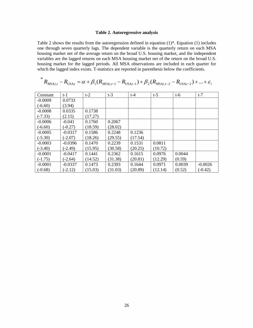
Next, we test for the return persistence in the MSA indices using the autoregressive

analysis from equation (1). The AR results are reported in table 2 for up to seven quarterly lags.

The explanatory power of the lagged returns is positive and significant for all lags between two

and five quarters. Surprisingly, the first period’s lag gradually turns negative and significant when

we increase the number of lags in the regression. The coefficients of the lags between two and

five periods are large in magnitude, statistically significant, and much larger than the first

periods’ negative coefficients or coefficients of the lags greater than five quarters. The second,

third and fourth lag seem to have the largest explanatory power. The sixth lag is also positive, but

small in magnitude and not statistically significant7.

Overall, the results reported in table 2 provide support to hypothesis one. The results

suggest that areas with above (below) U.S. average return during quarters t-2 through t-5 are

likely to outperform (underperform) the average return on residential real estate in the U.S. during

quarter t. The results also hint of a slight mean-reverting effect that is taking place during quarter

t-1. To reaffirm the momentum evidence presented in tables 2, and to provide economic meaning

to the momentum effect, we present the long-short portfolio strategy results in table 3.

4.2. Momentum Using Long-Short Strategy

Table 3’s panels A, B, and C show the annualized returns on long portfolios using

equation (2), short portfolios using equation (3), and zero cost long-short portfolios derived from

equation (4). The zero cost portfolios are formed based on lagged returns from one to four

quarters and are held for one to four quarters before rebalancing. The sample consists of quarterly

returns on the MSAs’ indices from the first quarter of 1983 to the third quarter of 2008.

7 The specification suggested by the AIC is an AR model with five lags.

16

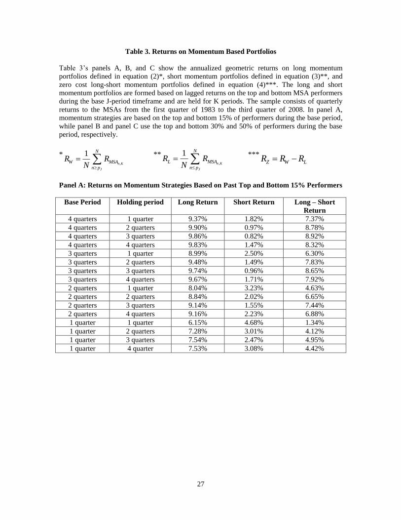
In panel A, the long portfolio buys housing indices that are lagged J-quarters’ winners, or

in the top 15% performers of the U.S. MSAs available to us at that time. Similarly, the short

portfolio sells housing indices that were lagged J-quarters’ losers, or in the bottom 15%

performers of the U.S. MSAs of the sample. The long portfolios’ average annualized return varies

from 6.15% to 9.90%. The highest long return (9.90%) is generated by the portfolio that buys

winners based on four quarters returns and holds the index for two quarters. The least profitable

long portfolio (6.15%) buys winners based on one quarter’s returns and holds the indices for one

quarter.

Short portfolios generate positive annualized returns in all base-holding period

combinations. However, these returns are always lower compared to their long portfolio

counterparts. The short portfolios’ returns range from 0.82% to 4.68%. The lowest short return

(0.82%) is generated by the portfolio that sells losers based on past four quarters’ returns and

holds the indices for three quarters. The highest short portfolio return (4.68%) is in the portfolio

that shorts losers based on their one quarter return and holds them for one quarter.

Returns on zero cost long-short portfolios that are constructed based on momentum

strategy range from 1.34% to 8.92% on an annual basis. From the combinations tested, the

strategy that buys and shorts housing indices based on one quarter’s return and holds them for one

quarter performs the worst, while the combination that buys and shorts housing indices based on

four quarters’ return and holds them for three quarters performs the best. Overall, panel A’s

results suggest that when holding the base period constant, the abnormal returns increase with the

holding period from one to two to three quarters, but are slightly lower for four quarter holding

periods compare to three quarter holding periods. Also, while holding the holding period

constant, the abnormal return increases with a longer base period. The positive, consistent, and

economically significant abnormal returns generated by the momentum based zero cost portfolios

supports our hypothesis 2.

17

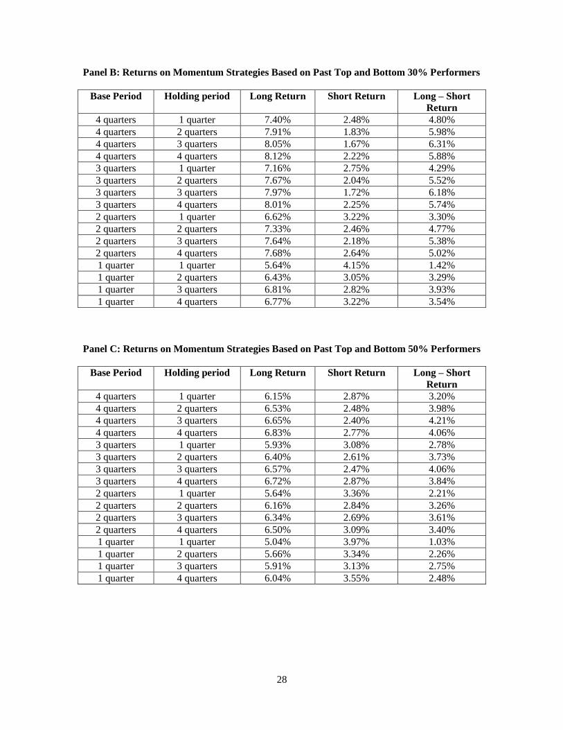
In panel B the analysis is repeated from panel A, except that instead of the 15% cutoffs

for winners and losers, we use the top 30% and bottom 30% of the MSA indices to construct the

buy and sell portfolios. The long portfolios’ average annualized returns range from 5.64% to

8.12%. The highest long return (8.12%) is generated by the portfolio that buys winners based on

four quarters returns and holds the index for four quarters. The least profitable long portfolio

(5.64%) buys winners based on one quarter’s returns and holds the indices for one quarter. The

results are smaller in magnitude compared to panel A, but behave similarly across different base-

holding period combinations, so that the highest long returns are generated by portfolios that have

longer base and holding periods.

Short portfolios generate positive annualized returns in all base-holding period

combinations similarly to panel A. The short portfolios’ returns range from 1.67% to 4.15%. The

lowest short return (1.67%) is generated by the portfolio that sells losers based on past four

quarters’ returns and holds the indices for three quarters. The highest short portfolio return

(4.15%) is in the portfolio that shorts losers based on their one quarter return and holds them for

one quarter. Again, these are the same base-holding periods that generate the highest and lowest

returns in panel A for the long and short portfolios.

Returns on zero cost long-short portfolios range from 1.42% to 6.31% on an annual basis.

From all combinations, the strategy that buys and shorts housing indices based on one quarter’s

return and holds them for one quarter performs the worst, while the combination that buys and

shorts housing indices based on four quarters’ return and holds them for three quarters performs

the best. These are again the same portfolios that produced the highest and lowest long-short

returns in panel A. Also, the results suggest that when holding the base period constant, the

abnormal returns increase with the holding period from one to two to three quarters, but are

slightly lower for four quarter holding periods compared to three quarter holding periods. Finally,

while holding the holding period constant, the abnormal return increases with a longer base

period. The findings provide more support for our hypothesis 2.

18

Finally, in panel C we repeat the analysis from panels A and B with 50% cutoffs for

determining winners and losers of the MSA indices to construct the buy and sell portfolios. The

long portfolios’ average annualized returns vary from 5.04% to 6.83% and the short portfolios’

returns range from 2.40% to 3.97%. The highest and lowest returns for both long and short

portfolios are generated by the same portfolios from panel B.

Returns on zero cost long-short portfolios range from 1.03% to 4.21% on an annual basis.

Again, similar to panels A and B, the strategy that buys and shorts housing indices based on one

quarter’s return and holds them for one quarter performs the worst, while the combination that

buys and shorts housing indices based on four quarters’ return and holds them for three quarters

performs the best. The results also suggest that the abnormal returns increase with longer holding

period and longer base period.

Figures 1 to 3 illustrate performance of the best performing long-short portfolios that buy

winners and sell losers based on their four quarters lagged return and hold the winning and losing

indices for three quarters after which the portfolios are rebalanced. Figure 1 shows the 15th

percentile cutoff results, figure 2 shows the 30th percentile, and figure 3 the 50

th percentile cutoffs

of winner and loser MSA indices.

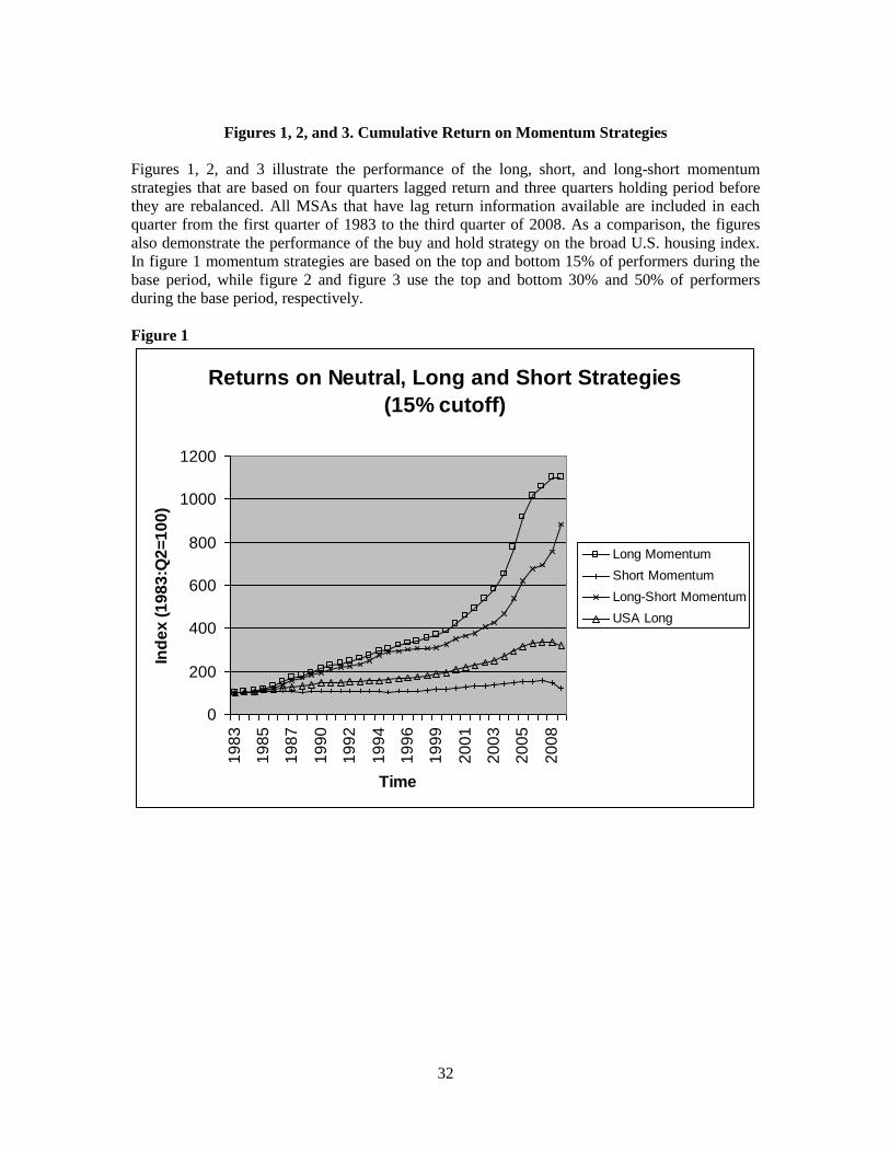
In figure 1, since 1983 the long-short zero investment portfolio accumulated almost an

800% return compared to the US housing index that generated just over 220% return over the

same time period. Note however, that the roughly 220% generated by the U.S. housing index is a

simple buy and hold long strategy. As a comparison, the long momentum based portfolio returned

roughly 1000% over the same time period.

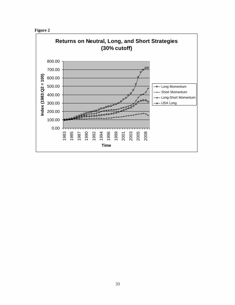
In figure 2, since 1983 the long-short zero investment portfolio accumulated almost

400% return and the long momentum based portfolio returned over 600% over the same time

period. Smaller accumulated return for the momentum portfolios is shown in figure 3. The long-

short zero investment portfolio accumulated nearly 200% return and the long momentum based

portfolio returned roughly 400% over the same time period. Once again, both figure 2 and figure

19

3 show that momentum based strategies outperform traditional buy and hold investment

strategies.

Overall, the findings support hypotheses 1 and 2, that there exists positive momentum in

the housing markets, and that zero investment long-short portfolios are able to produce positive

and economically significant abnormal returns. The zero investment long-short portfolios

generate up to 8.92% on an annual basis. The magnitude of this return is especially impressive

when compared to the buy and hold return on the U.S. housing index, which during the same

period is 4.69% per annum. The abnormal returns are increasing with the holding period and base

period, and the highest abnormal returns are produced by a strategy that uses 15th percentile

cutoffs in determining the winning and losing MSAs based on their lagged returns. The abnormal

returns are lower for strategies that use 30th percentile cutoff and the lowest for strategies that use

50th percentile as the cutoff points in forming long-short portfolios.

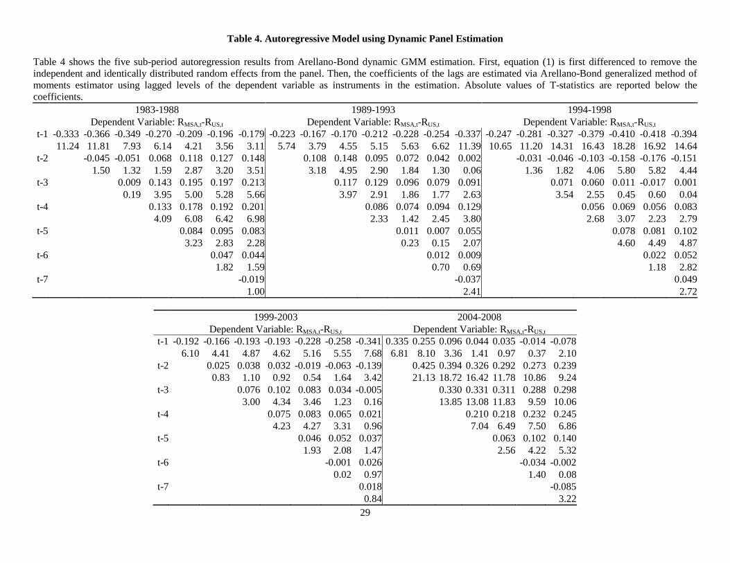
4.3. Robustness Checks

Table 4 reports results from the dynamic GMM estimation for five sub-periods (1983-

1988, 1989-1993, 1994-1998, 1999-2003, and 2004-2008)8. The results are similar in nature to

the results presented in table 2. Lags t-2 to t-4 are generally positive, statistically significant, and

large in magnitude during all sub-periods. However, their magnitude and significance level is

especially large during the 2004-2008 time period, and also during this time period the first

quarter’s negative return is much smaller in magnitude or even positive depending on the

specification. These results are consistent with our initial AR analysis that momentum is present

in all time periods, while showing that momentum is stronger during the later time period9.

8 Results of the full sample Arellano-Bond estimation are similar to our autoregression results. We do not

include the results for brevity, and they are available upon request. 9 The results from the full sample Arellano-Bond dynamic GMM estimation are very similar to the results

in table 2 in both significance and magnitude.

20

Table 5 presents the results of a long-short strategy for the five consecutive 5-year sub-

periods spanning the full 25 year sample. Building on the results from table 3, we construct our

long-short portfolios based on previous 4 quarters returns and a holding period of 3 quarters. We

again use top and bottom 15%, 30%, and 50% cutoff to identify winners and losers. Overall, the

results show that momentum in real estate is not unique to particular time period. Also, similar to

what is shown in table 3, a stricter definition of previous winners and losers (top and bottom

15%) yields higher return compared with a more relaxed definition (top and bottom 50%).

Even though the results show positive housing price momentum in all sub-periods, the

magnitude of the momentum is not constant across time. The momentum profits are higher in the

early and the late part of the sample and lower in the middle. The long-short strategy yields an

annual geometric return of as high as 14.88% during the 2004-2008 period and 10.79% during the

1983-1988 period. The returns during the 1989-1993 and 1999-2003 periods are still high, but

less than 8%, and the return during the 1994-1998 period is lower than 4.50% annually.

Table 6 displays the yield earned on the long-short portfolios in four different regions of

the U.S.. The results show the robustness of the momentum effect in housing prices subject to

geographical segmentation, but once again, with different magnitudes. The return on a

momentum based zero cost portfolio is highest in the West region (up to 10.02% annually) and

lowest in the Midwest region (up to 2.35% annually). The annual return on the momentum based

portfolio in the Northeast and the South is as high as 7.70% and 4.50% respectively. It appears

that areas in which home prices are higher and more volatile on average (West and Northeast)

have a stronger momentum effect compared with less expensive and volatile regions such as the

South and the Midwest.

5. Conclusion

21

Since Case and Shiller (1989), there have been several papers that document a positive

relationship between lagged returns and current returns in housing markets. Housing returns are

forecastable and there is strong evidence that housing markets, because of the transactions costs

and the nature of buyers and sellers participating in them, are probably less efficient than more

liquid markets with large institutional investors.

Our first contribution is documenting the momentum effect in a broad sample of housing

price indices in the U.S. over a long time period. Our dataset includes more than 380

Metropolitan Statistical Areas (MSAs). On average, quarterly MSA-specific lagged housing

returns over the U.S. lagged housing return are positively related to current MSA housing returns

over the U.S. housing return returns. This positive relation begins, as early as five quarters prior

to the current quarter with some signs of mean-reversion during the most recent quarter.

Similar to Jegadeesh and Titman’s (1993) stock market momentum paper, we form long-

short portfolios of the housing indices. We construct the buy portfolio from winning housing

markets and the short portfolio from losing housing markets based on their lagged returns. The

returns from the long-short portfolios are statistically significant and economically meaningful.

The annualized returns from these zero cost long-short portfolios are as high as 8.92% on an

annual basis. Such rate of return is about twice as large in magnitude compared with the return on

a traditional buy and hold strategy that is based on the broad US housing market index during the

same time period.

Our finding also confirms that the momentum effect in home prices exists regardless of

the time period or geographical region. However, the effect appears to be more pronounced in the

West and Northeast regions and during the 2004-2008 time period.

In reality, buying and selling of all of the housing indices used in this paper is not

possible as a tradable strategy. However, the Chicago Mercantile Exchange has tradable futures

on the major U.S. housing indices based on larger geographical areas, so there may be

opportunities for profitable trading strategies. Additionally, information about return momentum

22

and relative strength in housing can be useful for builders, potential home owners, and mortgage

originators.

23

6. References

Abraham, Jesse M. and Patric H. Hendershott (1993). Patterns and Determinants of Metropolitan

House Prices, 1977-1991, Real Estate and Credit Crunch, 18-42.

Abraham, Jesse M. and Patric H. Hendershott (1996). Bubbles in Metropolitan Housing Markets,

Journal of Housing Research 7(2), 191-207.

Ali, Ashiq and Mark Trombley (2006). Short Sales Constraints and Momentum in Stock Returns,

Journal of Business Finance & Accounting 33(3-4), 587-615.

Ang, Andrew, Robert J. Hodrick, Yuhang Xing, and Xiaoyan Zhang (2006). The Cross-Section

of Volatility and Expected Returns, Journal of Finance 61(1), 259-299.

Arellano, Manuel and Stephen Bond (1991). Some Tests of Specification for Panel Data: Monte

Carlo Evidence and an Application to Employment Equations, The Review of Economic

Studies 58, 277-297.

Atteberry, William L., Ronald C. Rutherford, and Mark E. Eakin (1993). Industrial Real Estate

Prices and Market Efficiency, Journal of Real Estate Research 8(3), 377-386.

Bloomfield, Robert J., Robert Libby, and Mark W. Nelson (1999). Confidence and the Welfare of

Less-Informed Investors, Accounting, Organizations and Society 24(8), 623-647(25).

Brounen, Dirk (2008). The Boom and Gloom of Real Estate Markets, Working Paper.

Calhoun, Charles A. (1996). OFHEO House Price Indices: HPI Technical Description, Office of

Federal Housing Enterprise Oversight.

Carhart, Mark M. (1997). On Persistence in Mutual Fund Performance, Journal of Finance 52(1),

57-82.

Case, Karl E. and Robert J. Shiller (1989). The Efficiency of the Market for Single-Family

Homes, American Economic Review 79(1), 125-137.

Case, Karl E. and Robert J. Shiller (1990). Forecasting Prices and Excess Returns in the Housing

Market, Real Estate Economics 18(3), 253-273.

Chan, Louis K., Narasimhan Jegadeesh, and Josef Lakonishok (1996). Momentum Strategies,

Journal of Finance 51(5), 1681-1711.

Chui, A. C. W., S. Titman, and K.C.J. Wei (2003). Intra-industry Momentum: The Case of

REITs, Journal of Financial Markets 6, 363-387.

Chui, A. C. W., S. Titman, and K.C.J. Wei (2008). Individualism and Momentum around the

World, Working paper.

Clayton, Jim (2003). Rational Expectations, Market Fundamentals and Housing Price Volatility,

Real Estate Economics 24(4), 441-470.

Daniel, Kent, David Hirschleifer, and Avanidhar Subrahmanyam (1998). Investor Psychology

and Security Market Under- and Overreactions, Journal of Finance 53, 1839-1886.

De Bondt Werner F. M. and Richard Thaler (1985). Does the Stock Market Overreact?, Journal

of Finance, 40(3), 793-805.

Fu Ng (2001). Market Efficiency and Return Statistics: Evidence from Real Estate and Stock

Markets Using a Present Value Approach, Real Estate Economics 29(2), 227-250.

Gau, George W. (1984). Weak Form Tests of the Efficiency of Real Estate Investment Markets,

Financial Review 19(4), 301-320.

24

Gau, George W. (1987). Efficient Real Estate Markets: Paradox or Paradigm, Real Estate

Economics 15(2), 1-12.

Gervais, Simon and Terrance Odean (2001). Learning To Be Overconfident, Review of Financial

Studies 14, 1-27.

Goetzmann, William N. and Roger R. Ibbotson (1994). Do Winners repeat? Patterns in Mutual

Fund Performance, Journal of Portfolio Management 20, 9-18.

Green, William H. (2003). Econometric Analysis (5th edition), Upper Saddle River, NJ: Prentice

Hall.

Gupta, Rangan and Stephen M. Miller (2008). “Ripple Effects” and Forecasting Home Prices in

Los Angeles, Las Vegas, and Phoenix, Working Paper.

Hamilton, B and R. Schwab (1995). Expected Appreciation in Urban Housing Markets, Journal

of Urban Economics 18, 103-118

Hendricks, Darryll, Jayendu Patel, and Richard Zeckhauser (1993). Hot Hands in Mutual Funds:

Short-Run Persistence of Performance, 1974-1988, Journal of Finance 48, 93-130.

Hung, Kathy and John L. Glascock (2009). Volatilities and Momentum Returns in Real Estate

Investment Trusts, Working Paper.

Hung, Kathy and John L. Glascock (2008). Momentum Profitability and Market Trend: Evidence

from REITs, Journal of Real Estate Finance and Economics 37, 51-69.

Jegadeesh, Narasimhan and Sheridan Titman (1993). Returns to Buying Winners and Selling

Losers: Implications for Stock market Efficiency, Journal of Finance 48(1), 65-91.

Jegadeesh, Narasimhan and Sheridan Titman (2001). Profitability of Momentum Strategies: An

Evaluation of Alternative Explanations, Journal of Finance 56, 699-720.

Lakonishok Josef, Andrei Shleifer, and Robert W. Vishny (1994). Contrarian Investment,

Extrapolation, and Risk, Journal of Finance 49(5), 1541-1578.

Lee, Charles M.C. and Bhaskaran Swaminathan (2000). Price Momentum and Trading Volume,

Journal of Finance 55(5), 2017-2069.

Levy, Robert (1967). Relative Strength as a Criterion for Investment selection, Journal of

Finance 22, 595-610.

Linneman, P. (1986). An Empirical Test of the Efficiency of the Housing Market, Journal of

Urban Economics 20, 140-154.

Piazzesi, Monika and Martin Schneider (2009). Momentum Traders in the Housing Market:

Survey Evidence and a Search Model, NBER Working Paper 14669.

Rouwenhorst, Geert K. (1998). International Momentum Strategies, Journal of Finance 53(1),

267-284.

Shiller, Robert J. (2007). Understanding Recent Trends in House Prices and Home Ownership.

NBER Working Paper.

Shiller, Robert J. (2008). Historic Turning Points in Real Estate, Eastern Economic Journal 34, 1-

13.

Zhang, X. Frank (2006). Information Uncertainty and Stock Returns, Journal of Finance 61(1),

105-137.

25

Table 1. Descriptive Statistics of MSAs’ Historical Housing Returns

Table 1 shows selected descriptive statistics of Metropolitan Statistical Areas’ (MSAs) housing

returns during the sample period from the first quarter of 1983 to third quarter in 2008. The

average annual appreciation as well as the standard deviation are for the broad U.S. housing index

during the sample period. The average annual appreciations for the top and bottom 15%, 30%,

and 50% are based on hindsight selection of MSAs.

Number of MSAs 1983 181

Number of MSAs 2008 381

Avg. annual appreciation 83-08 – U.S. 4.69%

Stdv. annual appreciation 83-08 – U.S. 3.41%

Avg. annual appreciation 83-08 – Top 15% (Hindsight) 6.39%

Avg. annual appreciation 83-08 – Bottom 15% (Hindsight) 2.67%





26

Table 2. Autoregressive analysis

Table 2 shows the results from the autoregression defined in equation (1)*. Equation (1) includes

one through seven quarterly lags. The dependent variable is the quarterly return on each MSA

housing market net of the average return on the broad U.S. housing market, and the independent

variables are the lagged returns on each MSA housing market net of the return on the broad U.S.

housing market for the lagged periods. All MSA observations are included in each quarter for

which the lagged index exists. T-statistics are reported in parenthesis below the coefficients.

*

itUSAtiMSAtUSAtiMSAtUSAtiMSA RRRRRR ...)()( 2,2,,21,1,,1,,,

Constant t-1 t-2 t-3 t-4 t-5 t-6 t-7

-0.0009

(-6.60)

0.0733

(3.94)

-0.0008

(-7.33)

0.0335

(2.15)

0.1738

(17.27)

-0.0006

(-6.60)

-0.041

(-0.27)

0.1760

(18.59)

0.2067

(28.02)

-0.0005

(-5.30)

-0.0317

(-2.07)

0.1586

(18.26)

0.2248

(29.55)

0.1236

(17.54)

-0.0003

(-3.40)

-0.0396

(-2.49)

0.1470

(15.95)

0.2239

(30.58)

0.1531

(20.25)

0.0811

(10.72)

-0.0001

(-1.75)

-0.0417

(-2.64)

0.1441

(14.52)

0.2362

(31.38)

0.1615

(20.81)

0.0976

(12.29)

0.0044

(0.59)

-0.0001

(-0.68)

-0.0337

(-2.12)

0.1473

(15.03)

0.2393

(31.03)

0.1644

(20.89)

0.0971

(12.14)

0.0039

(0.52)

-0.0026

(-0.42)

27

Table 3. Returns on Momentum Based Portfolios

Table 3’s panels A, B, and C show the annualized geometric returns on long momentum

portfolios defined in equation (2)*, short momentum portfolios defined in equation (3)**, and

zero cost long-short momentum portfolios defined in equation (4)***. The long and short

momentum portfolios are formed based on lagged returns on the top and bottom MSA performers

during the base J-period timeframe and are held for K periods. The sample consists of quarterly

returns to the MSAs from the first quarter of 1983 to the third quarter of 2008. In panel A,

momentum strategies are based on the top and bottom 15% of performers during the base period,

while panel B and panel C use the top and bottom 30% and 50% of performers during the base

period, respectively.

*,

1n K

J

N

W MSA

n p

R RN

**

,

1n K

J

N

L MSA

n p

R RN

***

Z W LR R R

Panel A: Returns on Momentum Strategies Based on Past Top and Bottom 15% Performers

Base Period Holding period Long Return Short Return Long – Short

Return

4 quarters 1 quarter 9.37% 1.82% 7.37%

4 quarters 2 quarters 9.90% 0.97% 8.78%











1 quarter 1 quarter 6.15% 4.68% 1.34%

1 quarter 2 quarters 7.28% 3.01% 4.12%


1 quarter 4 quarter 7.53% 3.08% 4.42%

28

Panel B: Returns on Momentum Strategies Based on Past Top and Bottom 30% Performers


Return













1 quarter 1 quarter 5.64% 4.15% 1.42%




Panel C: Returns on Momentum Strategies Based on Past Top and Bottom 50% Performers


Return













1 quarter 1 quarter 5.04% 3.97% 1.03%




29

Table 4. Autoregressive Model using Dynamic Panel Estimation

Table 4 shows the five sub-period autoregression results from Arellano-Bond dynamic GMM estimation. First, equation (1) is first differenced to remove the

independent and identically distributed random effects from the panel. Then, the coefficients of the lags are estimated via Arellano-Bond generalized method of

moments estimator using lagged levels of the dependent variable as instruments in the estimation. Absolute values of T-statistics are reported below the

coefficients.

1983-1988 1989-1993 1994-1998

Dependent Variable: RMSA,t-RUS,t Dependent Variable: RMSA,t-RUS,t Dependent Variable: RMSA,t-RUS,t

t-1 -0.333 -0.366 -0.349 -0.270 -0.209 -0.196 -0.179 -0.223 -0.167 -0.170 -0.212 -0.228 -0.254 -0.337 -0.247 -0.281 -0.327 -0.379 -0.410 -0.418 -0.394

11.24 11.81 7.93 6.14 4.21 3.56 3.11 5.74 3.79 4.55 5.15 5.63 6.62 11.39 10.65 11.20 14.31 16.43 18.28 16.92 14.64

t-2 -0.045 -0.051 0.068 0.118 0.127 0.148 0.108 0.148 0.095 0.072 0.042 0.002 -0.031 -0.046 -0.103 -0.158 -0.176 -0.151

1.50 1.32 1.59 2.87 3.20 3.51 3.18 4.95 2.90 1.84 1.30 0.06 1.36 1.82 4.06 5.80 5.82 4.44

t-3 0.009 0.143 0.195 0.197 0.213 0.117 0.129 0.096 0.079 0.091 0.071 0.060 0.011 -0.017 0.001

0.19 3.95 5.00 5.28 5.66 3.97 2.91 1.86 1.77 2.63 3.54 2.55 0.45 0.60 0.04

t-4 0.133 0.178 0.192 0.201 0.086 0.074 0.094 0.129 0.056 0.069 0.056 0.083

4.09 6.08 6.42 6.98 2.33 1.42 2.45 3.80 2.68 3.07 2.23 2.79

t-5 0.084 0.095 0.083 0.011 0.007 0.055 0.078 0.081 0.102

3.23 2.83 2.28 0.23 0.15 2.07 4.60 4.49 4.87

t-6 0.047 0.044 0.012 0.009 0.022 0.052

1.82 1.59 0.70 0.69 1.18 2.82

t-7 -0.019 -0.037 0.049

1.00 2.41 2.72

1999-2003 2004-2008

Dependent Variable: RMSA,t-RUS,t Dependent Variable: RMSA,t-RUS,t

t-1 -0.192 -0.166 -0.193 -0.193 -0.228 -0.258 -0.341 0.335 0.255 0.096 0.044 0.035 -0.014 -0.078

6.10 4.41 4.87 4.62 5.16 5.55 7.68 6.81 8.10 3.36 1.41 0.97 0.37 2.10

t-2 0.025 0.038 0.032 -0.019 -0.063 -0.139 0.425 0.394 0.326 0.292 0.273 0.239

0.83 1.10 0.92 0.54 1.64 3.42 21.13 18.72 16.42 11.78 10.86 9.24

t-3 0.076 0.102 0.083 0.034 -0.005 0.330 0.331 0.311 0.288 0.298

3.00 4.34 3.46 1.23 0.16 13.85 13.08 11.83 9.59 10.06

t-4 0.075 0.083 0.065 0.021 0.210 0.218 0.232 0.245

4.23 4.27 3.31 0.96 7.04 6.49 7.50 6.86

t-5 0.046 0.052 0.037 0.063 0.102 0.140

1.93 2.08 1.47 2.56 4.22 5.32

t-6 -0.001 0.026 -0.034 -0.002

0.02 0.97 1.40 0.08

t-7 0.018 -0.085

0.84 3.22

30

Table 5. Sub-Period Returns on Momentum Based Portfolios

Table 4 shows the sub-period annualized geometric returns on long momentum portfolios defined

in equation (2)*, short momentum portfolios defined in equation (3)**, and zero cost long-short

momentum portfolios defined in equation (4)***. The long and short momentum portfolios are

formed based on lagged returns on the top and bottom MSA performers during the base J=4

periods timeframe and are held for K=3 periods. The 25 years (1983 to 2008) covered by the data

are divided into five consecutive 5-year periods.

*,

1n K

J

N

W MSA

n p

R RN

**

,

1n K

J

N

L MSA

n p

R RN

***

Z W LR R R

Sub-period Cutoff for

Winners/Losers

Long Return Short Return Long – Short

Return

1983-1988 15% 12.04% 1.15% 10.79%

1983-1988 30% 9.11% 1.73% 6.31%

1983-1988 50% 7.19% 2.47% 4.69%

1989-1993 15% 8.02% 0.64% 7.38%

1989-1993 30% 6.46% 1.45% 7.33%

1989-1993 50% 5.47% 1.98% 3.46%

1994-1998 15% 5.92% 1.37% 4.44%

1994-1998 30% 5.29% 1.88% 4.99%

1994-1998 50% 4.89% 2.58% 2.28%

1999-2003 15% 11.49% 3.47% 7.95%

1999-2003 30% 9.12% 3.66% 3.34%

1999-2003 50% 7.35% 3.78% 3.54%

2004-2008 15% 12.96% -2.05% 14.88%

2004-2008 30% 11.15% -0.03% 11.14%

2004-2008 50% 8.94% 1.45% 7.46%

31

Table 6. Regional Analysis of Returns on Momentum Based Portfolios

Table 5 shows the annualized geometric returns momentum portfolios for four different

geographical regions. The long momentum portfolios defined in equation (2)*, short momentum

portfolios defined in equation (3)**, and zero cost long-short momentum portfolios defined in

equation (4)***. The long and short momentum portfolios are formed based on lagged returns on

the top and bottom MSA performers during the base J=4 periods timeframe and are held for K=3

periods. The sample consists of quarterly returns to the MSAs from the first quarter of 1983 to the

third quarter of 2008.

*,

1n K

J

N

W MSA

n p

R RN

**

,

1n K

J

N

L MSA

n p

R RN

***

Z W LR R R

Region Cutoff for

Winners/Losers

Long Return Short Return Long – Short

Return

Northeast 15% 9.92% 2.20% 7.70%

Northeast 30% 9.08% 2.72% 6.34%

Northeast 50% 8.12% 3.65% 4.46%

West 15% 10.38% 0.09% 10.02%

West 30% 9.64% 1.06% 8.40%

West 50% 8.22% 2.22% 5.87%

South 15% 6.31% 1.67% 4.50%

South 30% 5.69% 2.12% 3.52%

South 50% 4.97% 2.73% 2.20%

Midwest 15% 5.19% 2.79% 2.35%

Midwest 30% 4.96% 3.08% 1.86%

Midwest 50% 4.59% 3.26% 1.31%

32

Figures 1, 2, and 3. Cumulative Return on Momentum Strategies

Figures 1, 2, and 3 illustrate the performance of the long, short, and long-short momentum

strategies that are based on four quarters lagged return and three quarters holding period before

they are rebalanced. All MSAs that have lag return information available are included in each

quarter from the first quarter of 1983 to the third quarter of 2008. As a comparison, the figures

also demonstrate the performance of the buy and hold strategy on the broad U.S. housing index.

In figure 1 momentum strategies are based on the top and bottom 15% of performers during the

base period, while figure 2 and figure 3 use the top and bottom 30% and 50% of performers

during the base period, respectively.

Figure 1

Returns on Neutral, Long and Short Strategies

(15% cutoff)

0

200

400

600

800

1000

1200

19

83

19

85

19

87

19

90

19

92

19

94

19

96

19

99

20

01

20

03

20

05

20

08

Time

Ind

ex

(1

98

3:Q

2=

10

0)

Long Momentum

Short Momentum

Long-Short Momentum

USA Long

33

Figure 2

Returns on Neutral, Long, and Short Strategies

(30% cutoff)

0.00

100.00

200.00

300.00

400.00

500.00

600.00

700.00

800.001

98

3

19

85

19

87

19

90

19

92

19

94

19

96

19

99

20

01

20

03

20

05

20

08

Time

Ind

ex

(1

98

3:Q

2 =

10

0)

Long Momentum

Short Momentum

Long-Short Momentum

USA Long

34

Figure 3

Returns on Neutral, Long, and Short Strategies

(50% cutoff)

0

100

200

300

400

500

6001

98

3

19

85

19

87

19

90

19

92

19

94

19

96

19

99

20

01

20

03

20

05

20

08

Time

Ind

ex

(1

98

3:Q

2=

10

0)

Long Momentum

Short Momentum

Long-Short Momentum

USA Long

momentum in housing - uw · pdf filebeen shown to contribute to stock market momentum are ......

Documents