obstacle avoidance for a mobile robot - kth · the title, “obstacle avoidance for a mobile...
TRANSCRIPT
Obstacle Avoidance for a Mobile Robot
GUNNAR GULLSTRAND
Master’s Degree Project Stockholm, Sweden 2005
TRITA-NA-E05164
Numerisk analys och datalogi Department of Numerical Analysis KTH and Computer Science 100 44 Stockholm Royal Institute of Technology SE-100 44 Stockholm, Sweden
GUNNAR GULLSTRAND
TRITA-NA-E05164
Master’s Thesis in Computer Science (20 credits) at the School of Vehicle Engineering,
Royal Institute of Technology year 2005 Supervisor at Nada was Patric Jensfelt
Examiner was Henrik Christensen
Obstacle Avoidance for a Mobile Robot
ABSTRACT Obstacle Avoidance for a Mobile Robot A notorious problem in mobile obstacle avoidance is the detection and avoidance of obstacles. This thesis evaluates several well-known methods for controlling the motion of a mobile robot in an unknown dynamic environment. One of these methods, the Global Dynamic Window Approach, is selected and, using a laser range finder as the only range sensor, the method is implemented and tested on a mobile robot platform, a Pioneer 2 from ActivMedia. The result showed that the method is indeed an effective way for detecting and avoiding obstacles in real-time, in out-door tests the robot has traversed obstacle courses at velocities up to 1.2 metres per second. The method however showed to have some drawbacks; and should be combined with a higher-level algorithm that directs the robot to the best path.
SAMMANFATTNING Hinderundvikning för en mobil robot Denna rapport beskriver ett examensarbete utfört vid Centrum för Autonoma System, CAS, vid institutionen för numerisk analys och datalogi vid Kungliga Tekniska Högskolan. Målet med examensarbetet var att välja ut och implementera en metod för hinderundvikning för en mobil robot. Rapporten inleds med en bakgrund till robotik och sensorer. Därefter beskrivs ett antal olika metoder för hinderundvikning. En av dessa metoder, the Global Dynamic Window Approach, är utvald och testad på en av de mobila plattformarna vid CAS. Resultaten presenterade här visar att algoritmen är en bra metod till hinderundvikning, i tester gjorda utomhus har plattformen åkt igenom en hinderbana i hastigheter upp till 1.2 meter per sekund. Resultaten i denna rapport bygger på att roboten använder en laser skanner som sin enda avståndsmätare, resultaten är inte nödvändigtvis samma som om andra sensorer hade använts. Tyvärr är inte metoden helt fulländad, i slutet av rapporten diskuteras hur den skulle kunna kombineras med ett beteende på hög nivå som ger metoden anvisningar om t.ex. vägval.
ACKNOWLEDGEMENTS A completed task is always preceded by a chain of events. All of which we are not in control or even aware of. Many actions have guided me towards completing this thesis. Some dating back to when my parents persuaded me to study when I was young and some to when my thesis supervisor did the same a few years later. I cannot thank my family enough for the support and understanding. And I cannot thank my supervisor Patric Jensfelt enough for the hours of support and time to answer stupid questions. Without you the code would be nothing but a big segmentation fault and the thesis would have to wait a few more years. I would also like to express my sincere gratitude to Prof. Henrik I. Christensen and all the people at the Centre for Autonomous Systems. My time at CAS has been very pleasant and educational.
PREFACE This M.Sc. Project has been carried out at the Centre for Autonomous Systems (CAS), which is a research centre at the Royal Institute of Technology in Stockholm. The centre does research in autonomous systems including mobile robot systems for manufacturing and domestic applications [23]. CAS has several robotic systems and some of them are presented in short in the appendix.
Assignment In mobile robotics one of the major areas of concern is how to control the robot’s movements, making the robot move without hitting any obstacles. The algorithm making these decisions is called an obstacle avoidance algorithm. The motivation for this thesis is to find a way to improve the obstacle avoidance algorithm that is in use at CAS. The current algorithm is built on a technique called the Vector Field Histogram, a method that has several inherent drawbacks, probably most serious of these is that it in no way considers the dynamics of the robot. A new way of controlling the robots was requested and I was given free reins, I was to do a literature study on the obstacle avoidance and implement the method that I found would yield the best result. The title, “Obstacle Avoidance for a Mobile Robot” well defines what this thesis is about, it is fairly easy to decide what is part of the thesis and what is not. Obstacle avoidance is however an important part of a robotic system, it is a big research field that had its peak a few years ago and many theories and methods have been put forth. It is not possible to present but a small subset of the different ideas here. The selected methods are however some of the more important ideas and studying them give a good understanding of obstacle avoidance. The requirements that were put on the algorithm were that it should be fast, robust and not dependent on prior information about the environment. It has to be fast for several reasons, firstly because a fast algorithm lets the robot react to changes in the environment quickly. It also means that the robot will be able to drive at higher velocities. Low computation time also lets several processes run concurrently on the CPU so that the robot can do more things than just avoid obstacles at the same time. Naturally the algorithm and especially the implementation also have to be robust. It is trusted to manoeuvre an expensive robot in environments where people and other robots are present so it must not fail, allowing the robot to collide. Nor can the algorithm depend on prior information since the surroundings can change quickly, furniture can be moved and people walk about. This information is not present in any map so the robot has to decide as it goes where it can drive.
TABLE OF CONTENTS 1. Introduction ..................................................................................................... 1
1.1. Robot behaviour....................................................................................... 1 1.2. Robot Architectures.................................................................................. 2 1.3. Avoiding obstacles ................................................................................... 3
2. Sensors and Actuators...................................................................................... 4
2.1. Sensors .................................................................................................... 4 2.2. Actuators ................................................................................................. 6
3. Representing the Environment.......................................................................... 8
3.1. Occupancy grid ........................................................................................ 9 4. Obstacle Avoidance ........................................................................................10
4.1. Potential fields ........................................................................................10 4.2. The Vector Field Histogram Method........................................................12 4.3. The Dynamic Window Approach.............................................................14 4.4. The Global Dynamic Window Approach .................................................17 4.5. Conclusion ..............................................................................................19
5. Algorithm.......................................................................................................20
5.1. The Map .................................................................................................20 5.2. The NF1..................................................................................................21 5.3. The GDWA.............................................................................................22
6. Experiments and Results .................................................................................24
6.1. The Map Size..........................................................................................24 6.2. The NF1..................................................................................................27 6.3. The GDWA.............................................................................................27 6.4. Outdoors .................................................................................................31 6.5. Conclusions ............................................................................................32
7. Summary and Conclusions..............................................................................33 8. Future Work ...................................................................................................34 References..........................................................................................................35
1
1. INTRODUCTION Mobile robot systems currently available on the market vary from autonomous dust-busters and lawnmowers to pet toys. Prices can in many cases seem a bit off-putting but low cost robots have started to surface on the market and more will certainly appear when robots start to exist in our every day life. The range of applications where robots can be useful is vast, anywhere where it is too dangerous for humans, too demanding or just too boring. In every robotic system the ability not to collide with objects but instead find an alternative path is not only central but also indeed a demand. Obstacle avoidance has been a research field since the first mobile robots saw daylight but had its peak a few years ago. This chapter is an introduction to the field of robotics and in part based on the book Behavior-Based Robotics by Ronald C. Arkin [2]. It gives a background to how we can build a system that lets a robot accomplish different tasks. In chapter 2 the sensors that are most commonly put on a robot are discussed. As we will see, they have limitations to what they can tell the robot. No matter what sensor is chosen, the robot cannot get very exact information about its environment. The key is to combine different sensors and remember their limitations. In 3, Representing the Environment, we discuss how the sensor data should be used so that the robot can extract accurate and reliable information. Some of the effect that the imperfect sensors have can be limited by representing the data in a clever way. Chapter 4 gets down to business and discusses the different methods of obstacle avoidance covered in this thesis. The chapter ends with a discussion of why the method selected was preferred. Chapter 5 describes the implementation of the selected method at high level. In 6, Experiments and Results, the method’s performance is examined in various tests both in- and outdoor. Chapter 7 summarises the results and some of the things that could improve the robot’s performance but not covered in this thesis are discussed in chapter 8.
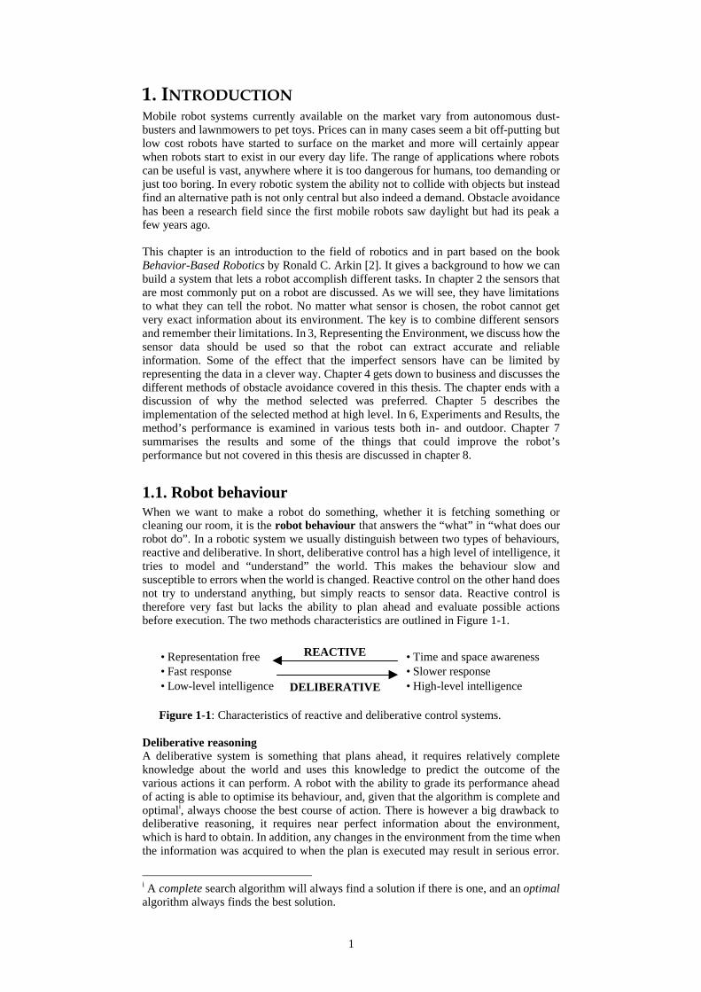
1.1. Robot behaviour When we want to make a robot do something, whether it is fetching something or cleaning our room, it is the robot behaviour that answers the “what” in “what does our robot do”. In a robotic system we usually distinguish between two types of behaviours, reactive and deliberative. In short, deliberative control has a high level of intelligence, it tries to model and “understand” the world. This makes the behaviour slow and susceptible to errors when the world is changed. Reactive control on the other hand does not try to understand anything, but simply reacts to sensor data. Reactive control is therefore very fast but lacks the ability to plan ahead and evaluate possible actions before execution. The two methods characteristics are outlined in Figure 1-1.
Figure 1-1: Characteristics of reactive and deliberative control systems. Deliberative reasoning A deliberative system is something that plans ahead, it requires relatively complete knowledge about the world and uses this knowledge to predict the outcome of the various actions it can perform. A robot with the ability to grade its performance ahead of acting is able to optimise its behaviour, and, given that the algorithm is complete and optimali, always choose the best course of action. There is however a big drawback to deliberative reasoning, it requires near perfect information about the environment, which is hard to obtain. In addition, any changes in the environment from the time when the information was acquired to when the plan is executed may result in serious error.
i A complete search algorithm will always find a solution if there is one, and an optimal algorithm always finds the best solution.
DELIBERATIVE
REACTIVE • Time and space awareness• Slower response • High-level intelligence
• Representation free • Fast response • Low-level intelligence
2
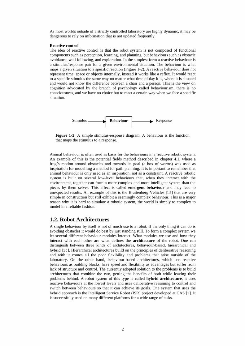
As most worlds outside of a strictly controlled laboratory are highly dynamic, it may be dangerous to rely on information that is not updated frequently. Reactive control The idea of reactive control is that the robot system is not composed of functional components such as perception, learning, and planning, but behaviours such as obstacle avoidance, wall following, and exploration. In the simplest form a reactive behaviour is a stimulus/response pair for a given environmental situation. The behaviour is what maps a given situation to a specific reaction (Figure 1-2). A reactive behaviour does not represent time, space or objects internally, instead it works like a reflex. It would react to a specific stimulus the same way no matter what time of day it is, where it is situated and would not know the difference between a chair and a person. This is the view on cognition advocated by the branch of psychology called behaviourism, there is no consciousness, and we have no choice but to react a certain way when we face a specific situation.
Figure 1-2: A simple stimulus-response diagram. A behaviour is the function that maps the stimulus to a response.
Animal behaviour is often used as basis for the behaviours in a reactive robotic system. An example of this is the potential fields method described in chapter 4.1, where a frog’s motion around obstacles and towards its goal (a box of worms) was used as inspiration for modelling a method for path planning. It is important to remember that animal behaviour is only used as an inspiration, not as a constraint. A reactive robotic system is built on several low-level behaviours that, when they interact with the environment, together can form a more complex and more intelligent system than the pieces by them selves. This effect is called emergent behaviour and may lead to unexpected results. An example of this is the Braitenberg Vehicles [15] that are very simple in construction but still exhibit a seemingly complex behaviour. This is a major reason why it is hard to simulate a robotic system, the world is simply to complex to model in a reliable fashion.
1.2. Robot Architectures A single behaviour by itself is not of much use to a robot. If the only thing it can do is avoiding obstacles it would do best by just standing still. To form a complex system we let several different behaviour modules interact. What modules we use and how they interact with each other are what defines the architecture of the robot. One can distinguish between three kinds of architectures, behaviour-based, hierarchical and hybrid [10]. Hierarchical architectures build on the principles of deliberative reasoning and with it comes all the poor flexibility and problems that arise outside of the laboratory. On the other hand, behaviour-based architectures, which use reactive behaviours as building blocks, have speed and flexibility as advantages but suffer from lack of structure and control. The currently adopted solution to the problems is to build architectures that combine the two, getting the benefits of both while leaving their problems behind. A robot system of this type is called hybrid architecture, it uses reactive behaviours at the lowest levels and uses deliberative reasoning to control and switch between behaviours so that it can achieve its goals. One system that uses the hybrid approach is the Intelligent Service Robot (ISR) project developed at CAS [1]. It is successfully used on many different platforms for a wide range of tasks.
Stimulus Response Behaviour
3
1.3. Avoiding obstacles In every mobile robotic system the skill to avoid obstacles is crucial. The robot must be trusted to complete its tasks without being a hazard to itself or other. The aim of this thesis is to survey the field of obstacle avoidance, select a suitable algorithm and implement it. The requirements that we have on the method is that it should be fast, robust and not dependent on prior information about the environment. Many methods to accomplish this have been put forth. They range from looking at a map and planning every move in advance to wandering about randomly without any planning at all. Naturally none of these extremes are preferable in robotic systems that should be reliable and accomplish various different tasks in dynamic environments. Instead we would like a method that would guide our robot the goal while still being able to quickly adapt to changes in its surroundings. One popular method for navigating the robot is to let the goal emit an attractive force and obstacles a repulsive force. By letting the robot get pulled along the gradient of the force field it will end up at the goal while avoiding obstacles. Problems with this approach include that there may be places where the force field cancel out, resulting in that the robot will stop, unable move in any direction. Another important part of obstacle avoidance is to consider the dynamics of the robot. This may not be a problem for slow robots but even at the speed of a brisk walk we will have to take this into account. The robot cannot just stop; it has to decelerate until it has stopped. One method that considers the dynamics of the robot is the Dynamic Window Approach (DWA). It calculates the velocities that the robot can achieve and selects the one that will get the robot on the best path to the goal. The method is purely functional, i.e. it does not consider the world in any other way than what the sensors see at the moment. This has the drawback that it cannot plan far ahead and that the robot can get stuck in certain obstacle configurations. This can be avoided by combining the DWA with a map over the environment, and using a local minima free search algorithm in it to find the path. This method is called the Global Dynamic Window Approach and was developed by Brock and Khatib [9].
4
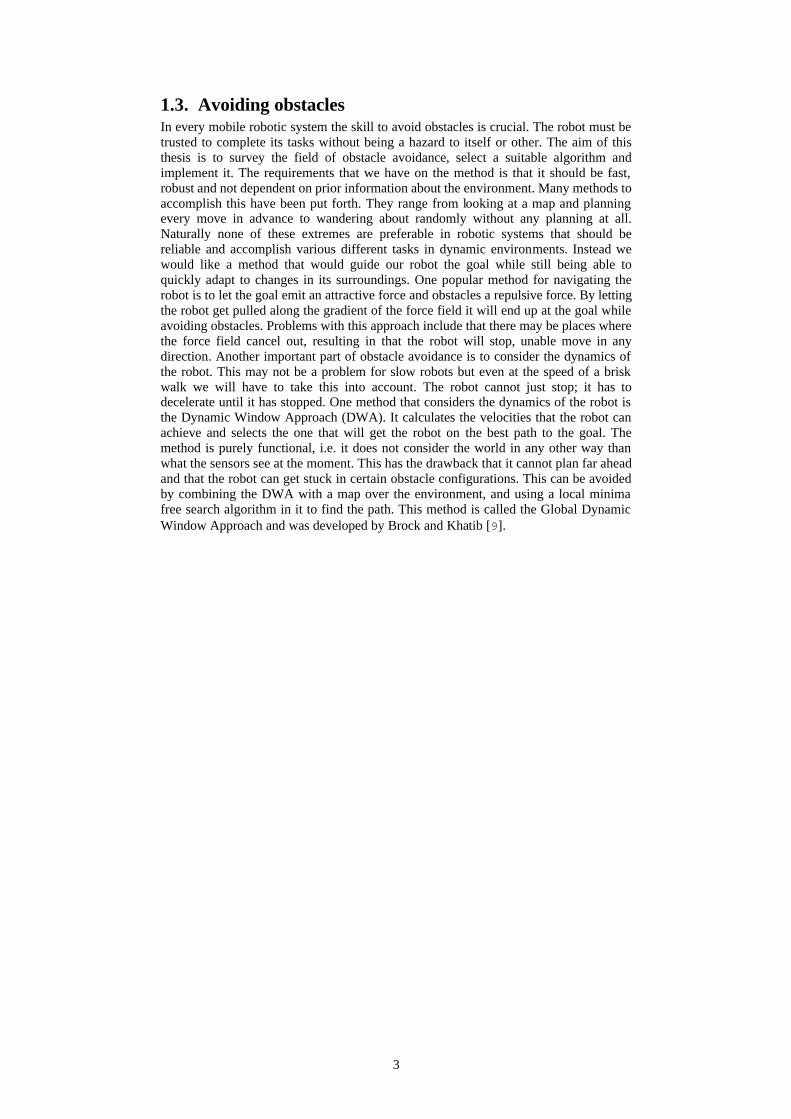
2. SENSORS AND ACTUATORS 2.1. Sensors In order to act in an unknown environment, a robot needs to obtain information about the world. This information is given by different kinds of sensors, just like we humans use our five senses. The sensors can be divided into two groups; internal and external. The internal sensors measure the internal state of the robot. This can for example be wheel encoders, measuring the rotation of the wheel axes. Examples of external sensors are cameras and radars. In the remainder of this section a brief presentation will be given of the most commonly used sensors for obstacle avoidance. In [12] a detailed description of sensors is given. Infrared sensors The infrared sensor works in the way that it sends out an IR-beam and measures the intensity of the reflected light. This makes the sensor highly material dependent. The reflected intensity can be several times bigger if the reflecting material is white plastic than if it is black cloth. The infrared sensors are also typically characterised by a highly limited range, usually less then one metre. The latter drawback makes it impractical to use, but the first drawback makes it virtually useless in a dynamic environment since the robot can never know what type of material it is looking at. As a consequence of the material dependency, the information given by the infrared sensor cannot be used to tell the distance to an object, merely tell if there is one or not in a certain direction. The reason for it being used at all is its low cost and very small size. For a small robot, such as the Kephera robot, where size does matter, it often is the main sensor. Ultra-sonic sensors The ultrasonic sensor is the most used sensor type, and almost all mobile robots today are equipped with them. The ultrasonic sensor works like the sonar of a bat. A pulse of sound is transmitted and the time until the reflection is received is measured. The distance to the reflecting object can then be calculated given the speed of sound. The maximum range is typically less than ten metres in open air, in water the range of the sensor is greatly increased. Just like the infrared sensor, the sonar sensor highly material dependent. Materials that are good sound absorbers limit the potential range significantly. The sound beam of the sensor will propagate like a cone, see Figure 2-1, and any object located in this cone will reflect the beam. This makes telling the exact position of the object hard. With a beam width of 25o, and a measured distance of two metres, the object can be anywhere on almost a metre wide arc. The wide beam is thus both a pro and a con, it easily detects obstacles but it is hard to tell exactly where they are.
Figure 2-1: A highly simplified model of the sound beam of a sonar sensor.
One great limitation of the sonar sensor is the effect called crosstalk. This happens when one sensor receives the emitted beam from another sensor. This is due to that all of the
5
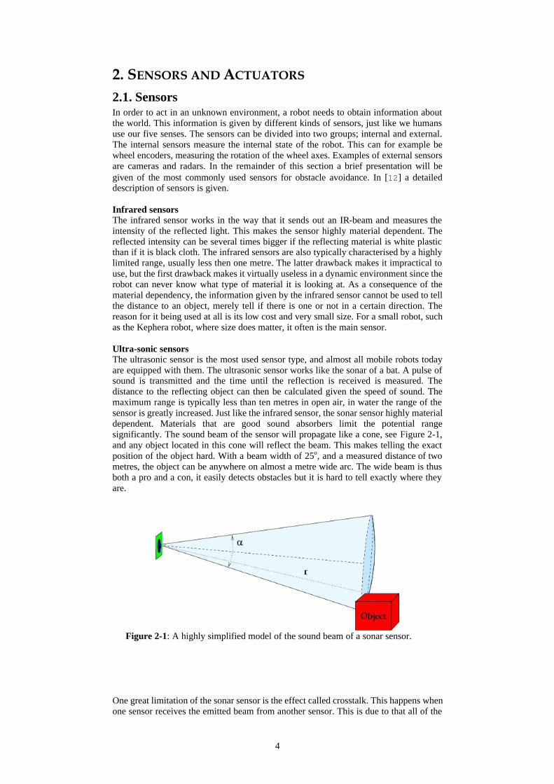
sensors use the same frequency for all transmitters/ receivers on the robot, which is the case on most commercially available platforms. To be able to reliably measure the distance to an object, it is necessary correctly associate the reflection with the correct transmission. A robot with many sonar sensors, see Figure 2-2, must therefore fire them sequentially, which limits the update frequency to around 3 Hz. Since most platforms use the same frequency, the association problem also occurs when several robots act in the same environment.
Figure 2-2: The sonar ring of a Nomad 200.
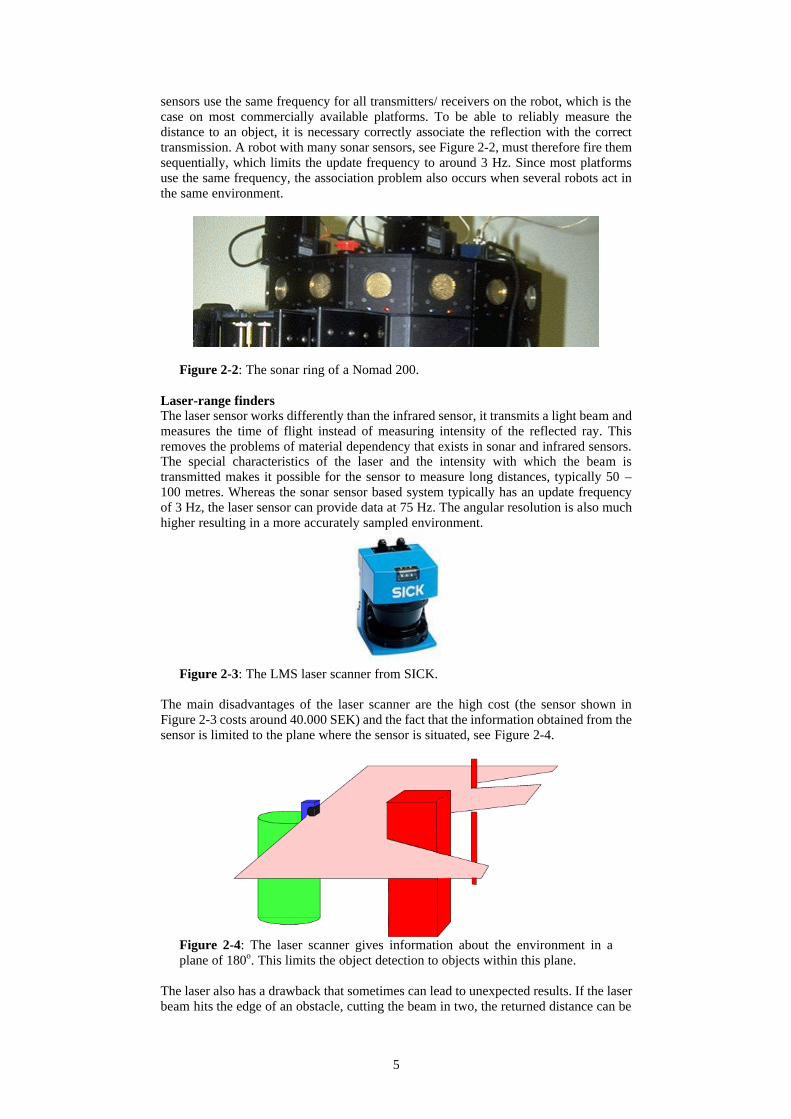
Laser-range finders The laser sensor works differently than the infrared sensor, it transmits a light beam and measures the time of flight instead of measuring intensity of the reflected ray. This removes the problems of material dependency that exists in sonar and infrared sensors. The special characteristics of the laser and the intensity with which the beam is transmitted makes it possible for the sensor to measure long distances, typically 50 – 100 metres. Whereas the sonar sensor based system typically has an update frequency of 3 Hz, the laser sensor can provide data at 75 Hz. The angular resolution is also much higher resulting in a more accurately sampled environment.
Figure 2-3: The LMS laser scanner from SICK.
The main disadvantages of the laser scanner are the high cost (the sensor shown in Figure 2-3 costs around 40.000 SEK) and the fact that the information obtained from the sensor is limited to the plane where the sensor is situated, see Figure 2-4.
Figure 2-4: The laser scanner gives information about the environment in a plane of 180o. This limits the object detection to objects within this plane.
The laser also has a drawback that sometimes can lead to unexpected results. If the laser beam hits the edge of an obstacle, cutting the beam in two, the returned distance can be
6
anywhere from the edge to the obstacle behind it. In Figure 2-5 this phenomenon is shown with a sketch and data from a real laser visualized in Matlab.
Figure 2-5: The laser sensor can sometimes return false range-readings if the laser beam hits the edge of an obstacle. The width of the laser beam in the figure is greatly exaggerated.
In Test A, described in chapter 6, Experiments and Results, this effect influenced the robot’s behaviour each time the test was run, keeping it from choosing a direct path towards the goal. Vision Vision is naturally one of the best methods of getting detailed information about the environment. It is however a nontrivial task to extract knowledge of obstacles and the connectivity of free space from an image. Nevertheless, since the late nineteen seventeen’s when the Stanford’s Cart/CMU Rover used stereo cameras to navigate about one meter every 15 minutes, computer vision made huge progress and is now fully usable as an way of guiding mobile robots motion. Although vision is an important research field for obstacle avoidance, it is beyond the scope of this thesis to deal with it.
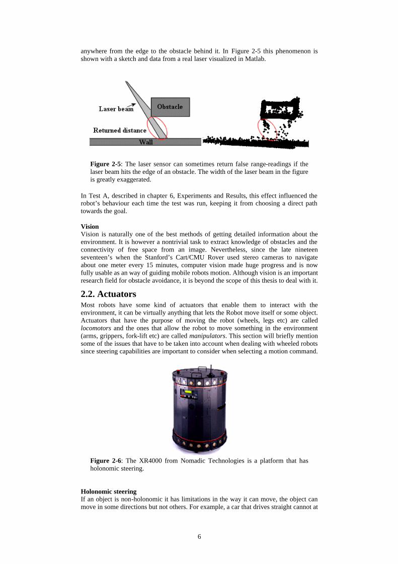
2.2. Actuators Most robots have some kind of actuators that enable them to interact with the environment, it can be virtually anything that lets the Robot move itself or some object. Actuators that have the purpose of moving the robot (wheels, legs etc) are called locomotors and the ones that allow the robot to move something in the environment (arms, grippers, fork-lift etc) are called manipulators. This section will briefly mention some of the issues that have to be taken into account when dealing with wheeled robots since steering capabilities are important to consider when selecting a motion command.
Figure 2-6: The XR4000 from Nomadic Technologies is a platform that has holonomic steering.
Holonomic steering If an object is non-holonomic it has limitations in the way it can move, the object can move in some directions but not others. For example, a car that drives straight cannot at
7
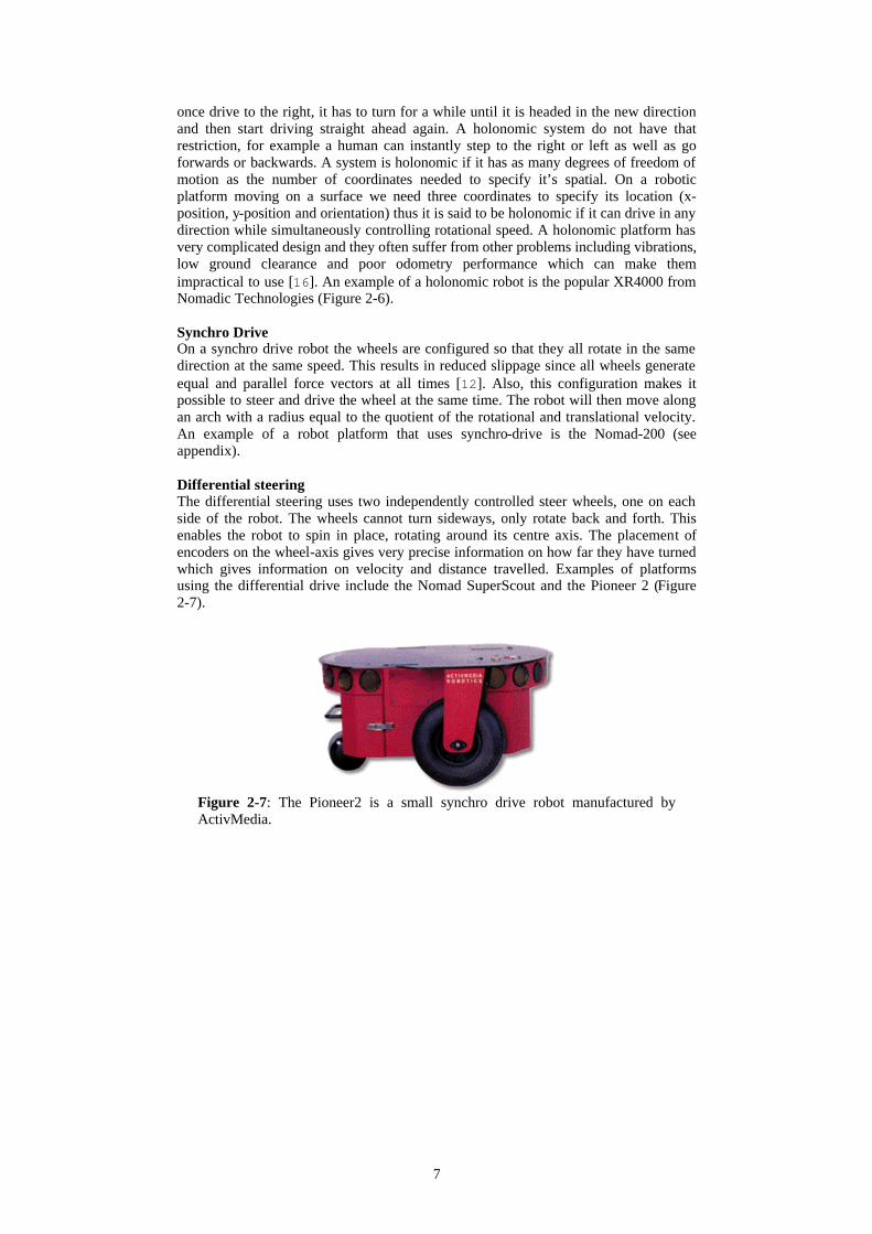
once drive to the right, it has to turn for a while until it is headed in the new direction and then start driving straight ahead again. A holonomic system do not have that restriction, for example a human can instantly step to the right or left as well as go forwards or backwards. A system is holonomic if it has as many degrees of freedom of motion as the number of coordinates needed to specify it’s spatial. On a robotic platform moving on a surface we need three coordinates to specify its location (x-position, y-position and orientation) thus it is said to be holonomic if it can drive in any direction while simultaneously controlling rotational speed. A holonomic platform has very complicated design and they often suffer from other problems including vibrations, low ground clearance and poor odometry performance which can make them impractical to use [16]. An example of a holonomic robot is the popular XR4000 from Nomadic Technologies (Figure 2-6). Synchro Drive On a synchro drive robot the wheels are configured so that they all rotate in the same direction at the same speed. This results in reduced slippage since all wheels generate equal and parallel force vectors at all times [12]. Also, this configuration makes it possible to steer and drive the wheel at the same time. The robot will then move along an arch with a radius equal to the quotient of the rotational and translational velocity. An example of a robot platform that uses synchro-drive is the Nomad-200 (see appendix). Differential steering The differential steering uses two independently controlled steer wheels, one on each side of the robot. The wheels cannot turn sideways, only rotate back and forth. This enables the robot to spin in place, rotating around its centre axis. The placement of encoders on the wheel-axis gives very precise information on how far they have turned which gives information on velocity and distance travelled. Examples of platforms using the differential drive include the Nomad SuperScout and the Pioneer 2 (Figure 2-7).
Figure 2-7: The Pioneer2 is a small synchro drive robot manufactured by ActivMedia.
8
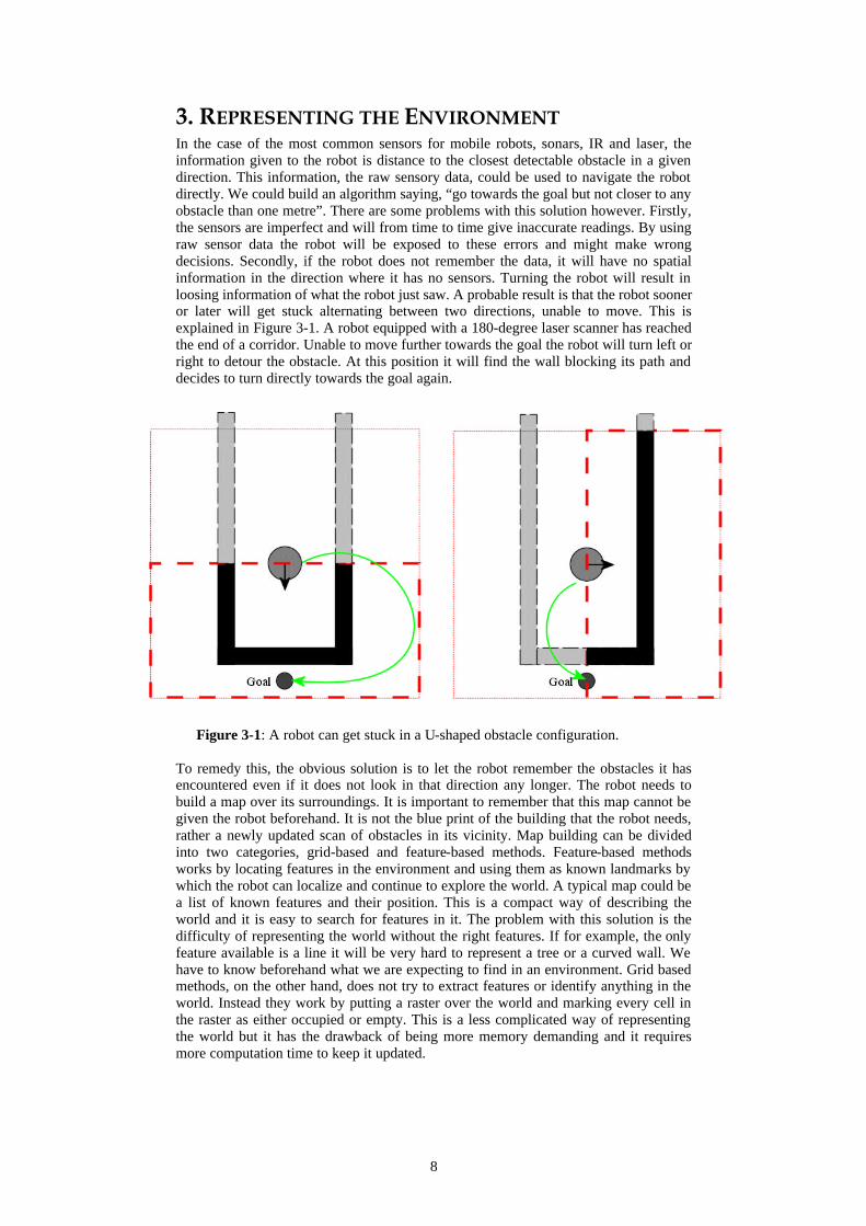
3. REPRESENTING THE ENVIRONMENT In the case of the most common sensors for mobile robots, sonars, IR and laser, the information given to the robot is distance to the closest detectable obstacle in a given direction. This information, the raw sensory data, could be used to navigate the robot directly. We could build an algorithm saying, “go towards the goal but not closer to any obstacle than one metre”. There are some problems with this solution however. Firstly, the sensors are imperfect and will from time to time give inaccurate readings. By using raw sensor data the robot will be exposed to these errors and might make wrong decisions. Secondly, if the robot does not remember the data, it will have no spatial information in the direction where it has no sensors. Turning the robot will result in loosing information of what the robot just saw. A probable result is that the robot sooner or later will get stuck alternating between two directions, unable to move. This is explained in Figure 3-1. A robot equipped with a 180-degree laser scanner has reached the end of a corridor. Unable to move further towards the goal the robot will turn left or right to detour the obstacle. At this position it will find the wall blocking its path and decides to turn directly towards the goal again.
Figure 3-1: A robot can get stuck in a U-shaped obstacle configuration.
To remedy this, the obvious solution is to let the robot remember the obstacles it has encountered even if it does not look in that direction any longer. The robot needs to build a map over its surroundings. It is important to remember that this map cannot be given the robot beforehand. It is not the blue print of the building that the robot needs, rather a newly updated scan of obstacles in its vicinity. Map building can be divided into two categories, grid-based and feature-based methods. Feature-based methods works by locating features in the environment and using them as known landmarks by which the robot can localize and continue to explore the world. A typical map could be a list of known features and their position. This is a compact way of describing the world and it is easy to search for features in it. The problem with this solution is the difficulty of representing the world without the right features. If for example, the only feature available is a line it will be very hard to represent a tree or a curved wall. We have to know beforehand what we are expecting to find in an environment. Grid based methods, on the other hand, does not try to extract features or identify anything in the world. Instead they work by putting a raster over the world and marking every cell in the raster as either occupied or empty. This is a less complicated way of representing the world but it has the drawback of being more memory demanding and it requires more computation time to keep it updated.
9
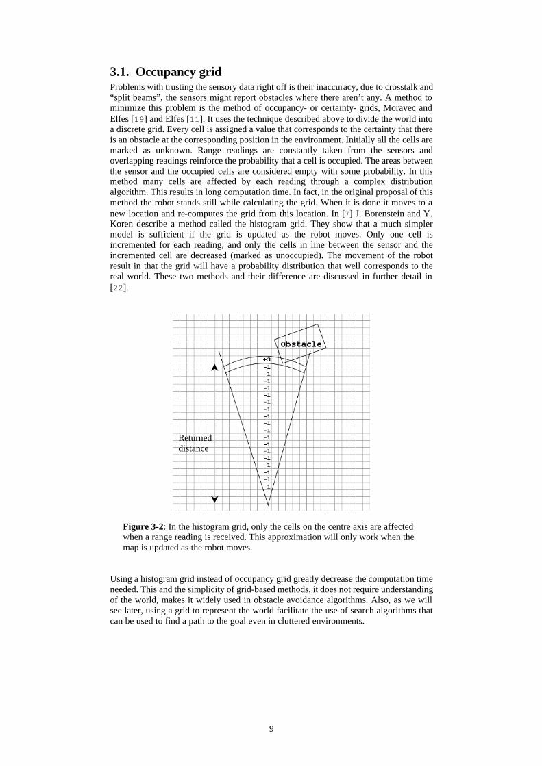
3.1. Occupancy grid Problems with trusting the sensory data right off is their inaccuracy, due to crosstalk and “split beams”, the sensors might report obstacles where there aren’t any. A method to minimize this problem is the method of occupancy- or certainty- grids, Moravec and Elfes [19] and Elfes [11]. It uses the technique described above to divide the world into a discrete grid. Every cell is assigned a value that corresponds to the certainty that there is an obstacle at the corresponding position in the environment. Initially all the cells are marked as unknown. Range readings are constantly taken from the sensors and overlapping readings reinforce the probability that a cell is occupied. The areas between the sensor and the occupied cells are considered empty with some probability. In this method many cells are affected by each reading through a complex distribution algorithm. This results in long computation time. In fact, in the original proposal of this method the robot stands still while calculating the grid. When it is done it moves to a new location and re-computes the grid from this location. In [7] J. Borenstein and Y. Koren describe a method called the histogram grid. They show that a much simpler model is sufficient if the grid is updated as the robot moves. Only one cell is incremented for each reading, and only the cells in line between the sensor and the incremented cell are decreased (marked as unoccupied). The movement of the robot result in that the grid will have a probability distribution that well corresponds to the real world. These two methods and their difference are discussed in further detail in [22].
Figure 3-2: In the histogram grid, only the cells on the centre axis are affected when a range reading is received. This approximation will only work when the map is updated as the robot moves.
Using a histogram grid instead of occupancy grid greatly decrease the computation time needed. This and the simplicity of grid-based methods, it does not require understanding of the world, makes it widely used in obstacle avoidance algorithms. Also, as we will see later, using a grid to represent the world facilitate the use of search algorithms that can be used to find a path to the goal even in cluttered environments.
Returned distance
10
4. OBSTACLE AVOIDANCE Obstacle avoidance is a key component in any mobile robotic system. If we want our system to move about in the real world we have to consider that there are obstacles not represented in any a priori map. The obstacles can either be static as for example a table or dynamic as a human or another robot. What we think of by obstacle avoidance is the ability to go from one place to another without running into things on the way. This means that obstacle avoidance is tightly coupled with path planning, it is not exactly the same thing but they depend on each other so much that they often are indistinguishable. In general, there are two kinds of methods for obstacle avoidance/ path planning, global and local. These build on the same ideas as the architectures mentioned earlier, a global obstacle avoidance algorithm requires a relative complete knowledge of the world and can compute the best path from start to goal offline. As this is practically impossible in a dynamic world (remember obstacles that are not in the map), the rest of this chapter will only concentrate on methods that relates to the local paradigm. These methods only consider what they “see” and act accordingly.
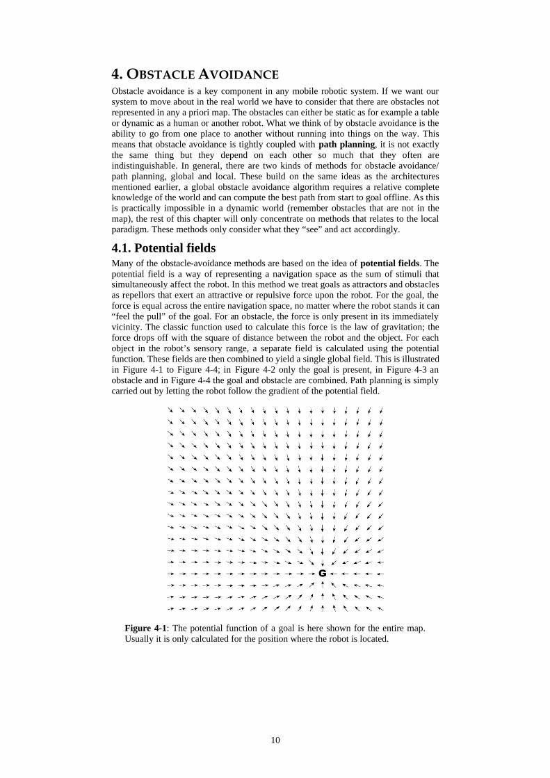
4.1. Potential fields Many of the obstacle-avoidance methods are based on the idea of potential fields. The potential field is a way of representing a navigation space as the sum of stimuli that simultaneously affect the robot. In this method we treat goals as attractors and obstacles as repellors that exert an attractive or repulsive force upon the robot. For the goal, the force is equal across the entire navigation space, no matter where the robot stands it can “feel the pull” of the goal. For an obstacle, the force is only present in its immediately vicinity. The classic function used to calculate this force is the law of gravitation; the force drops off with the square of distance between the robot and the object. For each object in the robot’s sensory range, a separate field is calculated using the potential function. These fields are then combined to yield a single global field. This is illustrated in Figure 4-1 to Figure 4-4; in Figure 4-2 only the goal is present, in Figure 4-3 an obstacle and in Figure 4-4 the goal and obstacle are combined. Path planning is simply carried out by letting the robot follow the gradient of the potential field.
Figure 4-1: The potential function of a goal is here shown for the entire map. Usually it is only calculated for the position where the robot is located.
11
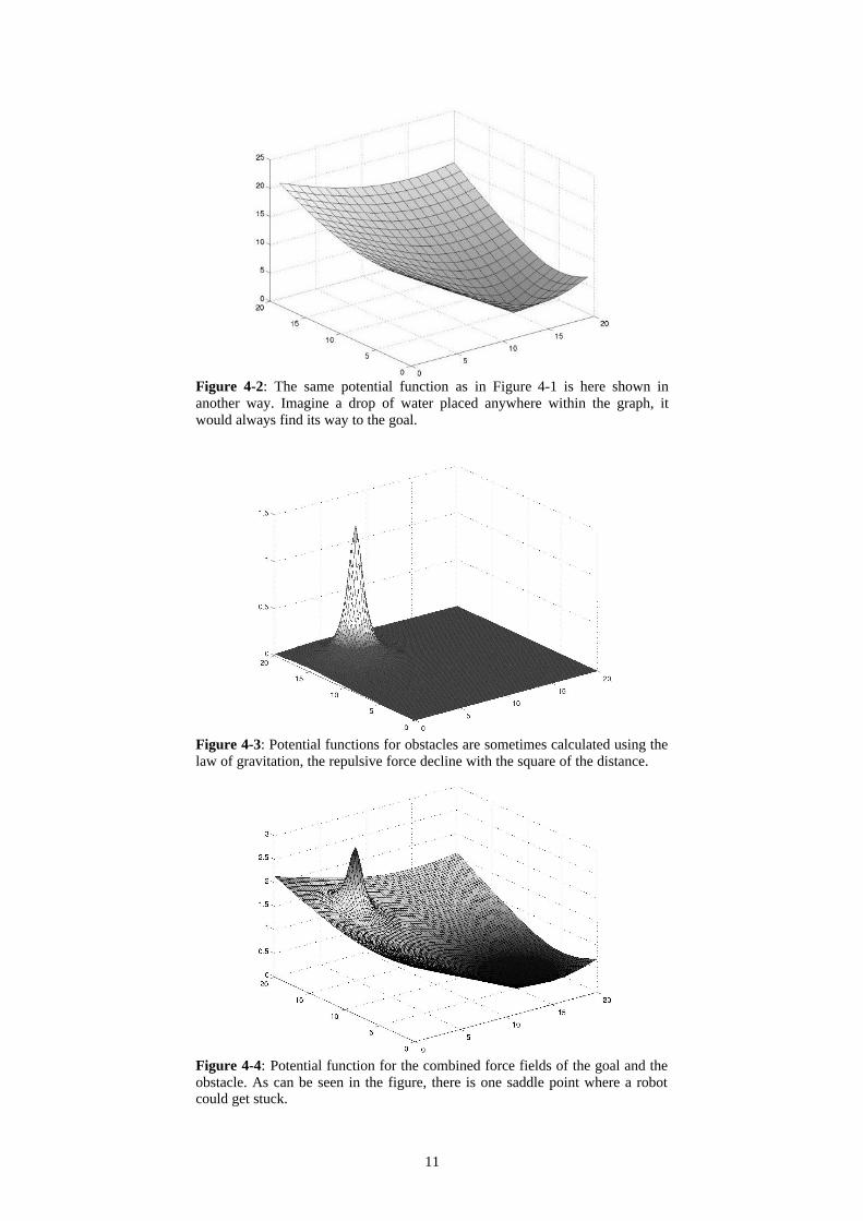
Figure 4-2: The same potential function as in Figure 4-1 is here shown in another way. Imagine a drop of water placed anywhere within the graph, it would always find its way to the goal.
Figure 4-3: Potential functions for obstacles are sometimes calculated using the law of gravitation, the repulsive force decline with the square of the distance.
Figure 4-4: Potential function for the combined force fields of the goal and the obstacle. As can be seen in the figure, there is one saddle point where a robot could get stuck.
12
A problem with the potential fields is the amount of time needed to compute the entire field of forces. This is avoided by only computing the forces that act upon the position where the robot currently is located. This has the effect that no global path planning is conducted at all, the robot merely reacts to the objects in its vicinity, resulting in a very fast method for obstacle avoidance. Unfortunately there are other problems with potential fields; Koren and Borenstein [17] identified some problems that are inherent to potential fields, i.e. they exist in all implementations of the method. The problems are:
• Trap situations due to local minima. Trap situations can occur when the robot runs into a U-shaped obstacle configuration. The force towards the goal will at some point inside the obstacle be equal to the force pointing away from the obstacle. Since there are obstacles on the side of the robot as well, the robot cannot simply turn around the obstacle and will likely be trapped. Trap-situations can be solved by global recovery, i.e. the robot needs to recognise the situation and recover by backtracking its travelled path until it can find another way. • No passage between closely spaced obstacles. This problem is similar to the previous one, if two obstacles are placed close to each other, like a doorframe, the repulsive forces from each obstacle is combined into a single repulsive force that points away from the opening between the obstacles. The robot will then turn away from the opening even if the goal is on the other side. • Oscillations in the presence of obstacles and in narrow passages. Borenstein and Koren also showed that the robot sometimes would oscillate in the presence of obstacles. This could for instance show itself when the robot travels in narrow corridors. When the robot is travelling along the centreline between the two walls, the motion is stable. If, however, the robot would drift closer to one of the walls it would be pushed back across the centreline by the repulsive force from the closest wall. The robot would now experience a repulsive force from the other wall and be pushed back across the centreline. This behaviour would then continue and the robot would oscillate between the two walls.
One implementation of the potential field approach is the Virtual Force Field method (J. Borenstein and Y. Koren [5]). Unfortunately it suffered from the problems listed above and was soon replaced with the Vector Field Histogram method described in the next section.
4.2. The Vector Field Histogram Method After identifying the problems with potential field methods, Koren and Borenstein continued their work by proposing a method that deals with the shortcomings of potential fields. In [6] they suggest a method for fast obstacle avoidance that they call the Vector Field Histogram (VFH). The method will only briefly be discussed here since it is not immediately related to the algorithm studied in this thesis. It is, however, an important method for obstacle avoidance and therefore worth mentioning. It is also the method that is currently used at CAS. The VFH method uses the histogram grid described above to represent the environment in which the robot travels. This makes the map fairly accurate even when the robot is equipped with sonars. The contents of each cell in the histogram grid is treated as an obstacle vector, the direction of the vector is the direction from the current position of the robot to the obstacle. The magnitude of the vector is given by a formula that considers both the certainty value of the cell and the distance to the cell (note that with a certainty value of zero the magnitude of the obstacle vector will also be zero).
13
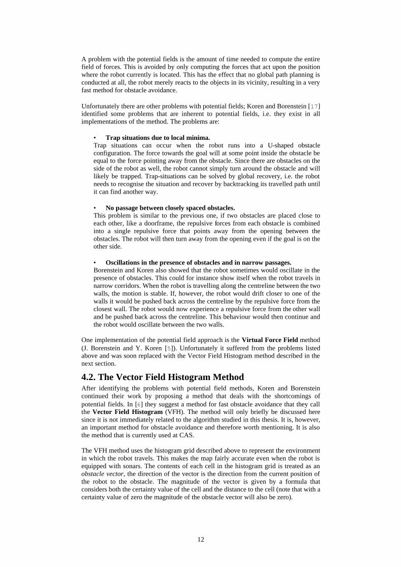
Next, the area surrounding the robot is divided into a number of equal sectors. In each sector the obstacle vectors of that sector are summed together to give the polar obstacle density (POD). In Figure 4-5 a typical robot environment and the resulting polar histogram is shown. As can be seen in the figure, a sector with a high POD, a “peak”, corresponds to obstacles nearby and low POD, a “valley”, corresponds to low obstacle density. In the figure of the environment, the sectors with high POD are marked as black, these sectors are unsafe for travel. Any valley with a POD below a certain threshold is considered safe and a candidate for travel. If there are more than one candidate valleys, the algorithm selects the one that most closely matches the direction to the target. Within this valley the sector that is mostly aligned with the target heading while letting the robot keep a safe clearance from obstacles is selected for travel.
Figure 4-5: The living room at CAS as the robot sees and the resulting polar histogram. The sectors marked as black around the robot corresponds to the peaks in the polar histogram. These sectors are unsafe for travel and not considered when choosing motion direction. The x in the lower left corner of the map represents the goal. As can be seen the robot cannot head directly towards it.
Experimental results of this method showed that most of the time the robot travelled at its maximum speed (0.78 m/s) without having to stop in order to calculate a safe path. The speed was only reduced when an obstacle was approached head-on. During these experiments, a 20-Mhz 80386 computer ran the VFH algorithm [6]. There are, however, some severe problems with this method.
• Dynamic constraints A thing that all the previously described systems have in common is that they all fail to take into account the dynamic constraints imposed on anything with a mass. A robot moving in full speed simply cannot make a 90-degree turn. Even if it does not fall over, it certainly will not stay on the calculated curvature. Nor can it stop at once if an obstacle suddenly appears in front of it, the laws of dynamics will keep the robot moving even if the wheels stop turning. In [21] the VFH method is augmented by taking the dynamics into account. The dynamic constraints imposed on the robot will block some of the sectors that were marked as free for travel in the original method.
14
• Parameter settings Another severe problem is the parameter setting, this is a problem that most algorithms have to deal with. In the VFH method the threshold that determines when a sector is save for travel defines the behaviour of the robot. A too low threshold will make the robot unable to move in the presence of obstacles, whereas a too large threshold will make the robot bump into the obstacles. What makes setting this parameter difficult is its lack of an intuitive interpretation.
As a response to the problems mentioned above, Bauer et al [4] introduce what they call the Steer Angle Field approach. Later on two similar methods were suggested, the Curvature-Velocity Method [20] and the Dynamic Window Approach (DWA) [13]. In this thesis, the DWA is presented in more detail.
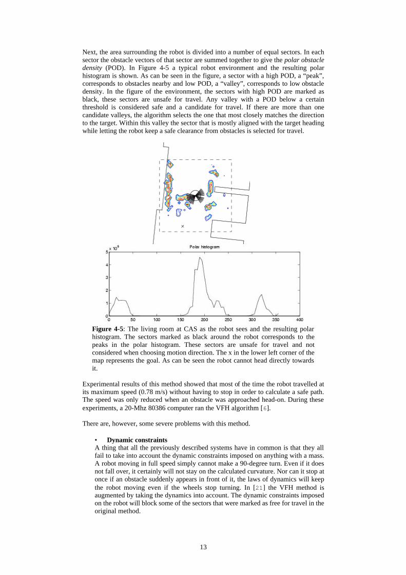
4.3. The Dynamic Window Approach Since no platforms are truly holonomic (see chapter 3) there are limitations as to which velocities the robot can achieve. The dynamic window approach is specially designed to deal with the dynamics of the robot by only considering those velocities. In the description that follows we will use the tuple (υ, ω) to represent the velocity of the robot. Here υ is the translational velocity and ω is the rotational velocity. Furthermore, only those trajectories that can be decomposed into circular arcs will be considered. When the robot is moving with a constant velocity, (υ, ω), it describes a circular motion with the radius υ/ω, see Figure 4-6. When ω is zero the robot travels on a straight line, this is a special case that has to be dealt with. The task at hand is to determine the best velocity at each point in time given kinematic and dynamic constraints of the robot and information about the surrounding environment.
Figure 4-6: The radius of a trajectory is given by the quota of the translational and rotational velocities.
Pruning the Search Space Finding the best velocity can be formulated as an optimisation problem of enormous complexity. To make the optimisation feasible, only a discrete set of velocities are considered. The outer bounds of this set are defined of the maximum velocity ( maxmax ,ων ) of the robot. To further prune the search space, velocities that are unsafe, i.e., leading to a collision, are marked as non-admissible and discarded from further calculations. The Dynamic Window To take the dynamics into account and also reduce the search space, only those velocities that can be reached within the next iteration, given the current velocity, are considered. These velocities form the so-called Dynamic Window. The size of the dynamic window is determined by the maximum acceleration ( maxmax ,ϖ&&v ).
15
Optimisation In essence, DWA combines three different behaviours (objectives) by a voting scheme. The different behaviours favour heading to goal, large distance to obstacles and high velocities. The behaviours grade each velocity in the dynamic window according to its preferences. The best velocity is given by maximising the following function over the set of possible and admissible velocities.
),(),(),(),( ϖγϖβϖαϖ vvelvdistvheadvG ⋅+⋅+⋅= Equation 4-1: The objective function of the DWA.
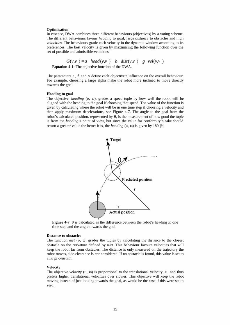
The parameters a , ß and γ define each objective’s influence on the overall behaviour. For example, choosing a large alpha make the robot more inclined to move directly towards the goal. Heading to goal The objective, heading (υ, ω), grades a speed tuple by how well the robot will be aligned with the heading to the goal if choosing that speed. The value of the function is given by calculating where the robot will be in one time step if choosing a velocity and then apply maximum decelerations, see Figure 4-7. The angle to the goal from the robot’s calculated position, represented by θ, is the measurement of how good the tuple is from the heading’s point of view, but since the value for conformity’s sake should return a greater value the better it is, the heading (υ, ω) is given by 180-|θ|.
Figure 4-7: θ is calculated as the difference between the robot’s heading in one time step and the angle towards the goal.
Distance to obstacles The function dist (υ, ω) grades the tuples by calculating the distance to the closest obstacle on the curvature defined by υ/ω. This behaviour favours velocities that will keep the robot far from obstacles. The distance is only measured on the trajectory the robot moves, side-clearance is not considered. If no obstacle is found, this value is set to a large constant. Velocity The objective velocity (υ, ω) is proportional to the translational velocity, υ, and thus prefers higher translational velocities over slower. This objective will keep the robot moving instead of just looking towards the goal, as would be the case if this were set to zero.
16
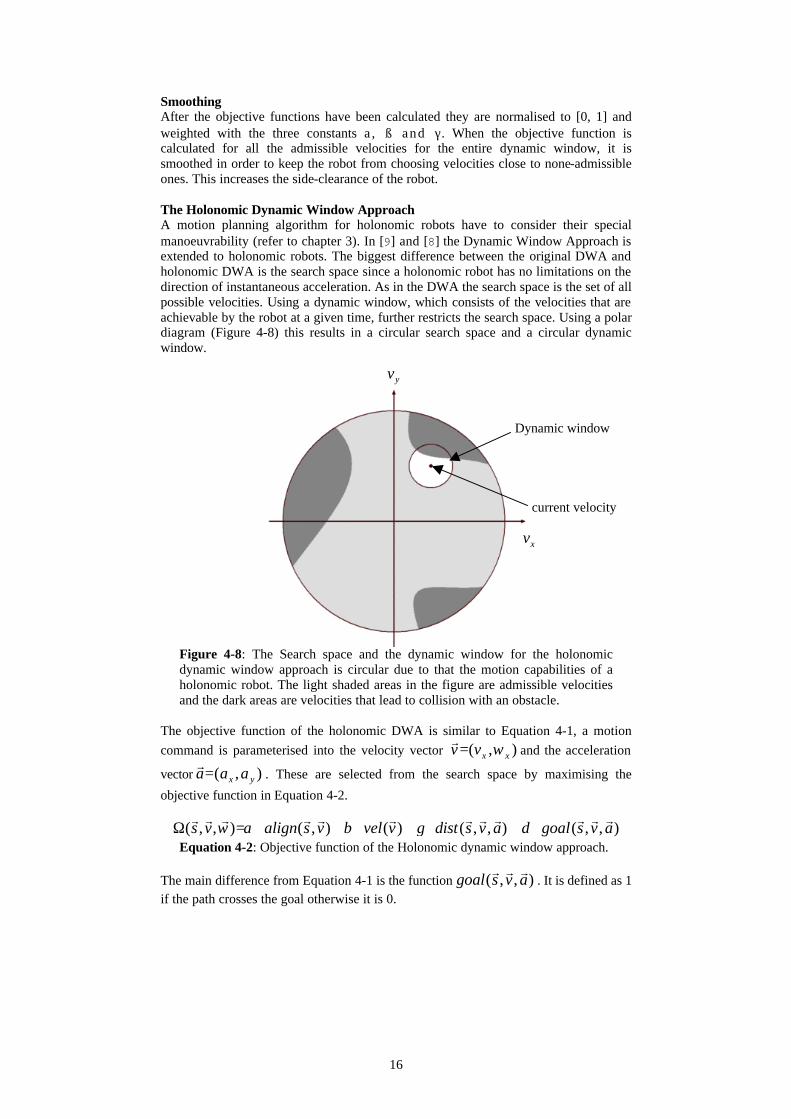
Smoothing After the objective functions have been calculated they are normalised to [0, 1] and weighted with the three constants a , ß and γ . When the objective function is calculated for all the admissible velocities for the entire dynamic window, it is smoothed in order to keep the robot from choosing velocities close to none-admissible ones. This increases the side-clearance of the robot. The Holonomic Dynamic Window Approach A motion planning algorithm for holonomic robots have to consider their special manoeuvrability (refer to chapter 3). In [9] and [8] the Dynamic Window Approach is extended to holonomic robots. The biggest difference between the original DWA and holonomic DWA is the search space since a holonomic robot has no limitations on the direction of instantaneous acceleration. As in the DWA the search space is the set of all possible velocities. Using a dynamic window, which consists of the velocities that are achievable by the robot at a given time, further restricts the search space. Using a polar diagram (Figure 4-8) this results in a circular search space and a circular dynamic window.
Figure 4-8: The Search space and the dynamic window for the holonomic dynamic window approach is circular due to that the motion capabilities of a holonomic robot. The light shaded areas in the figure are admissible velocities and the dark areas are velocities that lead to collision with an obstacle.
The objective function of the holonomic DWA is similar to Equation 4-1, a motion command is parameterised into the velocity vector ),( xxvv ω=
rand the acceleration
vector ),( yx aaa=r
. These are selected from the search space by maximising the
objective function in Equation 4-2.
),,(),,()(),(),,( avsgoalavsdistvvelvsalignvsrrrrrrrrrrrr
⋅+⋅+⋅+⋅=Ω δγβαω Equation 4-2: Objective function of the Holonomic dynamic window approach.
The main difference from Equation 4-1 is the function ),,( avsgoal
rrr. It is defined as 1
if the path crosses the goal otherwise it is 0.
Dynamic window
current velocity
xv
yv
17
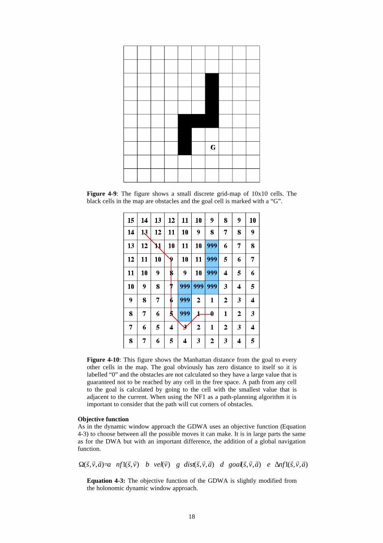
4.4. The Global Dynamic Window Approach As the DWA has no information about the connectivity of the free space it is, just like the potential field methods, susceptible to local minima. Brock and Khatib [9] suggest a method for obstacle avoidance, the Global Dynamic Window Approach GDWA, which extends the DWA and the Holonomic DWA with a simple motion-planning algorithm, i.e a function that finds a collision-free motion from the start configuration to the goal configuration. The motion-planning algorithm is fast enough to be computed in each iteration of the control-loop, which allows the robot to react in real-time while still using a global planner. Free space connectivity In order to plan a path in the environment, it has to be modelled in some way so that the robot can extract information about the connectivity of the free space from the model. The GDWA does not use a priori knowledge of the environment but samples it, using the robot’s sensors, and fuses the sensor information into a occupancy grid. Each reading from the sensors is treated as a point in R2 that contain an obstacle. The data is translated into configuration space by expanding the obstacles with the radius of the robot. This means that the robot can be represented as a point and this makes the path planning much simpler, if there is an unoccupied cell, then the robot will fit in it. This approach assumes that the robot is circular, otherwise another method should be used. Navigation function The idea of a navigation function is to find the best path from the robot to the goal. The best path is here defined as the shortest path, which is not necessarily the same as the fastest path. The GDWA uses the global, local minima free navigation function NF1 [18] to search the configuration space for the shortest path. This is done by calculating the Manhattan distance (moving like the tower in chess, not diagonally) from the goal cell to the robot. A formal description of the NF1 can be found in Algorithm 5-1, but in short it works like this; Start by initiating all cells to a large value and give the goal cell the value 0. Give every 1-neigbour of the goal that is in the free space the value 1. Continue by giving each cell in the free space their parent’s value plus one until there are no cells left. All the C-space obstacles will now have the value that all cells were initiated with while all cells in the free space will have their L1 value to the goal. An example of this can be seen in Figure 4-9 and Figure 4-10. A problem with the NF1 is that it grazes the C-obstacles. This is avoided in GDWA by only selecting motion commands that give the robot a minimum clearance to the obstacles. As the occupancy grid is recomputed in every cycle of the control loop, new obstacles added and old removed, the NF1 needs to be recomputed as well. This would be very costly if the NF1 was computed for the entire occupancy grid but the GDWA uses a different approach. The NF1 is only computed in a rectangle aligned with the goal heading. If the algorithm finds that there is an obstacle blocking its path, the width of the rectangle is increased until the robot is reached by the search front.
18
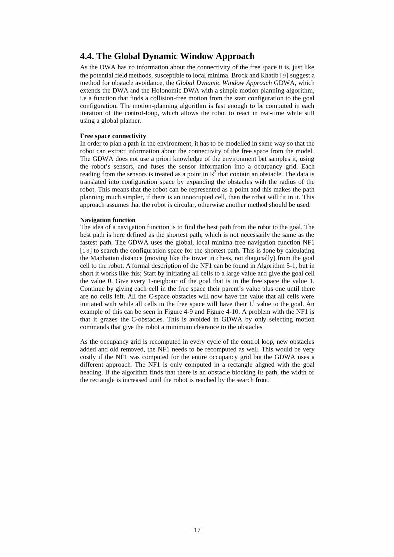
Figure 4-9: The figure shows a small discrete grid-map of 10x10 cells. The black cells in the map are obstacles and the goal cell is marked with a “G”.
Figure 4-10: This figure shows the Manhattan distance from the goal to every other cells in the map. The goal obviously has zero distance to itself so it is labelled “0” and the obstacles are not calculated so they have a large value that is guaranteed not to be reached by any cell in the free space. A path from any cell to the goal is calculated by going to the cell with the smallest value that is adjacent to the current. When using the NF1 as a path-planning algorithm it is important to consider that the path will cut corners of obstacles.
Objective function As in the dynamic window approach the GDWA uses an objective function (Equation 4-3) to choose between all the possible moves it can make. It is in large parts the same as for the DWA but with an important difference, the addition of a global navigation function.
),,(1),,(),,()(),(1),,( avsnfavsgoalavsdistvvelvsnfavsrrrrrrrrrrrrrrr
∆⋅+⋅+⋅+⋅+⋅=Ω εδγβα
Equation 4-3: The objective function of the GDWA is slightly modified from the holonomic dynamic window approach.
19
The function ),(1 vsnfrr
replaces the function ),( vsalignrr
from the holonomic dynamic window approach. The function is used to align the robot with the heading to the goal. Not the straight line to the goal but the path that nf1 found in the navigation function. The value of ),(1 vsnf
rr is calculated by comparing the value of the nf1 at the
cells that are adjacent to the robot’s position. Also the function ),,(1 avsnfrrr
∆ is added to the objective function. It indicates how much a motion command is expected to reduce the distance to the goal in the next iteration. Since the nf1 is not computed for the entire grid, there is a possibility that a motion command would bring the robot out of the computed region. In this case the GDWA uses the smallest potential value along that trajectory.
4.5. Conclusion The requirements we have on the obstacle avoidance algorithm are strict. In order of importance they are; no collisions, do not stand still, and high velocity. Naturally, no obstacle avoidance algorithm should collide. This puts high demands on accuracy and speed of detecting new obstacles. Nor should the algorithm let the robot stand still if there is a path to travel. Only if every possible path is blocked should the robot stop. This also requires that the map is accurate and prevents many simplifications. If the robot is oval it should not be modeled as a circle, since these extra few centimeters could be what allow it to travel a narrow path. The robot should also be allowed to travel as fast as possible. The velocity might be restricted for several reasons, but when it is possible to travel fast, it should not be the quality of the obstacle avoidance algorithm that restrains the velocity. This puts demands on the choice of algorithm as well as requires that we trust the map to be accurate. From the discussions in this chapter it should be clear that the GDWA is the best method of the ones described. It also satisfies the demands described above. By using the histogram grid for mapping it is fast and reliable in detecting dynamic obstacles. Rightly implemented it prevents collisions since these velocities should be marked as non-admissible. It does not stand still if there is some path that is non-blocked since high velocity is one of the objectives of the function. Lastly, in tests done, both in the articles referenced above and in this thesis, it has proven to be able to navigate obstacle courses traveling as fast as the platform allow. Based on these conclusions, the GDWA is chosen to be implemented and further tested.
20
5. ALGORITHM This chapter describes the GDWA in further detail. It does not cover the theoretical pars of the algorithm, rather it discusses on a high level how the algorithm was implemented. The solution that is presented here is, in the parts not described above, the authors own solution to how the GDWA should be implemented. The technique explained in this chapter does not necessarily match what is described in the original proposal of the GDWA. The algorithm consists of tree distinct parts that can be handled and described by them selves. The first is building the map. It is of necessity tightly coupled with obstacle avoidance so therefore it is included here. The second part is calculating the NF1. It could easily be included in the map algorithm but for modularity’s sake it is an independent component. The last but most complex part is calculating the actual motion command, the GDWA algorithm.
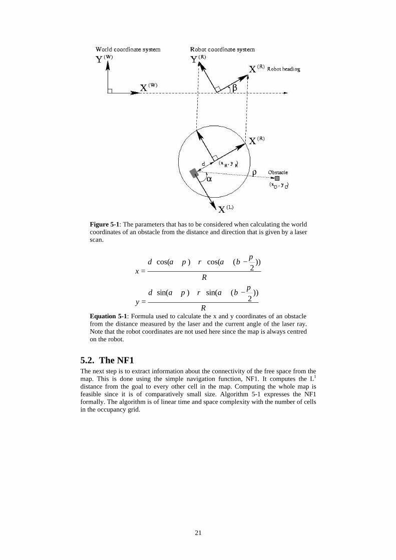
5.1. The Map The map uses the technique histogram grid (chapter 3.1) to merge sensor data and represent the world. The map is always centred on the robot. Whenever the robot moves, the map moves with it to centre on the robot’s new position. For simplicity the map is always aligned with the heading that the robot started in. The x-axis of the map will always be zero degrees in the odometry coordinate system. Moving the map has the disadvantage that objects in the map disappear as the robot moves away from it. The robot looses information that could have been used for path planning. On the other hand, it has the advantages that the map can be fairly small since the robot never will reach the end of it. A smaller map obviously saves computation time and memory usage. Nor is the loss of information a big problem, the map is not meant to be used for other things than obstacle avoidance. The data must be fresh and what the robot saw a few metres away might be out of date. After the map has been moved to its new position, new data is added to it. Since the data that arrives are on the form distance and heading, it has to be translated to the map’s coordinate system. The parameters to consider when adding laser data are shown in Figure 5-1 and the necessary calculation are shown in Equation 5-1. For sonar data the calculations are similar but the sensors are positioned in different ways. The cell found to be blocked gets its probability value updated. Depending on how big value is assigned it is considered more or less likely that it actually contain an obstacle. This value is different depending on what sensor that reports the obstacle. The laser is fairly accurate and has a narrow beam so it is trusted more than the sonar. When a cell is updated it is quite safe to assume that there are no obstacles between the sensor and the newly updated cell. These cells get their probability value slightly decreased. The sensors cannot remove each other’s obstacles, however. The sensors are usually mounted on different heights and therefore see different things, so the obstacles can only be removed by the sensor that added them. After the map is moved and obstacles are added, the map is aged. Every obstacle in the map has its probability value decreased. The obstacles that the robot constantly sees will not be affected since the ageing parameter is less than the adding parameter. It only affects the obstacles that the robot cannot see anymore. It was added so that a robot confined by obstacles should return to previously blocked places after a while to look for new openings.
21
Figure 5-1: The parameters that has to be considered when calculating the world coordinates of an obstacle from the distance and direction that is given by a laser scan.
R
dy
R
dx
))2
(sin()sin(
))2
(cos()cos(
πβαρπα
πβαρπα
−+⋅++⋅=
−+⋅++⋅=
Equation 5-1: Formula used to calculate the x and y coordinates of an obstacle from the distance measured by the laser and the current angle of the laser ray. Note that the robot coordinates are not used here since the map is always centred on the robot.
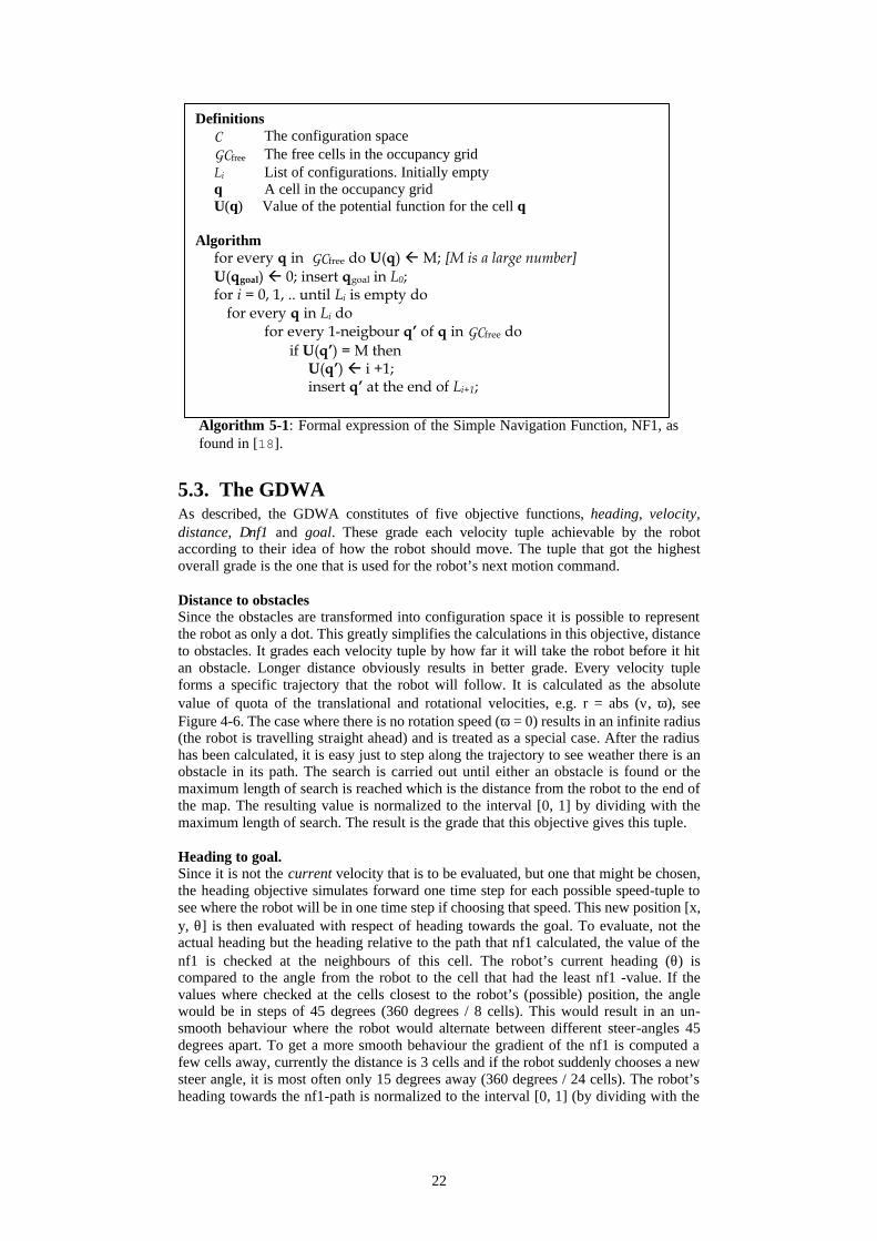
5.2. The NF1 The next step is to extract information about the connectivity of the free space from the map. This is done using the simple navigation function, NF1. It computes the L1 distance from the goal to every other cell in the map. Computing the whole map is feasible since it is of comparatively small size. Algorithm 5-1 expresses the NF1 formally. The algorithm is of linear time and space complexity with the number of cells in the occupancy grid.
22
Algorithm 5-1: Formal expression of the Simple Navigation Function, NF1, as found in [18].
5.3. The GDWA As described, the GDWA constitutes of five objective functions, heading, velocity, distance, ∆nf1 and goal. These grade each velocity tuple achievable by the robot according to their idea of how the robot should move. The tuple that got the highest overall grade is the one that is used for the robot’s next motion command. Distance to obstacles Since the obstacles are transformed into configuration space it is possible to represent the robot as only a dot. This greatly simplifies the calculations in this objective, distance to obstacles. It grades each velocity tuple by how far it will take the robot before it hit an obstacle. Longer distance obviously results in better grade. Every velocity tuple forms a specific trajectory that the robot will follow. It is calculated as the absolute value of quota of the translational and rotational velocities, e.g. r = abs (ν, ω), see Figure 4-6. The case where there is no rotation speed (ω = 0) results in an infinite radius (the robot is travelling straight ahead) and is treated as a special case. After the radius has been calculated, it is easy just to step along the trajectory to see weather there is an obstacle in its path. The search is carried out until either an obstacle is found or the maximum length of search is reached which is the distance from the robot to the end of the map. The resulting value is normalized to the interval [0, 1] by dividing with the maximum length of search. The result is the grade that this objective gives this tuple. Heading to goal. Since it is not the current velocity that is to be evaluated, but one that might be chosen, the heading objective simulates forward one time step for each possible speed-tuple to see where the robot will be in one time step if choosing that speed. This new position [x, y, θ] is then evaluated with respect of heading towards the goal. To evaluate, not the actual heading but the heading relative to the path that nf1 calculated, the value of the nf1 is checked at the neighbours of this cell. The robot’s current heading (θ) is compared to the angle from the robot to the cell that had the least nf1 -value. If the values where checked at the cells closest to the robot’s (possible) position, the angle would be in steps of 45 degrees (360 degrees / 8 cells). This would result in an un-smooth behaviour where the robot would alternate between different steer-angles 45 degrees apart. To get a more smooth behaviour the gradient of the nf1 is computed a few cells away, currently the distance is 3 cells and if the robot suddenly chooses a new steer angle, it is most often only 15 degrees away (360 degrees / 24 cells). The robot’s heading towards the nf1-path is normalized to the interval [0, 1] (by dividing with the
Definitions C The configuration space GCfree The free cells in the occupancy grid Li List of configurations. Initially empty q A cell in the occupancy grid U(q) Value of the potential function for the cell q
Algorithm
for every q in GCfree do U(q) ß M; [M is a large number] U(qgoal) ß 0; insert qgoal in L0; for i = 0, 1, .. until Li is empty do
for every q in Li do for every 1-neigbour q’ of q in GCfree do if U(q’) = M then U(q’) ß i +1; insert q’ at the end of Li+1;
23
biggest possible angle towards the goal; 180 degrees) and subtracted from 1 (0 angle to goal is better that 180). The result is returned as this objectives value on the speeds. Delta nf1 An important consideration when choosing speeds is, obviously, to choose a tuple that brings the robot closer to the goal. When computing the heading to goal objective, there might be velocities that bring the robot very aligned with the heading of the nf1 path, but at a position further away from the goal than another velocity might take it. This is compensated for by calculating the difference of nf1 between the robot’s current position and the one it will reach in one time step if choosing a certain tuple. This value is normalized [0, 1] by dividing it with the greatest value found in this iteration. Velocity The last of the objectives is the velocity. This is simply the translational velocity (v) normalized to [0, 1] by dividing with the maximum allowed velocity. This seems to mean that the robot always favours high velocity over slower, which is true, but the higher velocities are not always admissible. When the distance to obstacle objective has been calculated, the distance is compared to the breaking capabilities of the robot. If the speed in question is so big that the robot will not be able to stop before reaching the obstacle on the corresponding trajectory, it will be set to non-admissible. It is important to notice that, since the maximum length to search for obstacles is limited by the size of the map, the map size has influence on the maximum admissible velocity. The set of velocities are further pruned with respect to obstacle clearance. Once in each iteration the distance to the closest obstacle (in all directions) is considered and the maximum allowable speed is set linearly so that if the obstacle is very close, the speed is highly reduced, and at a distance of one metre, the obstacel is ignored (max speed allowed). This is not part of the original GDWA proposition made by Brooks, but was added partly to reduce the risk of hitting obstacles and partly to keep humans from getting scared by a fast moving (seemingly out-of-control) robot. Objective function After the different objectives have been calculated, the objective function of the dynamic window is calculated. It is simply computed by adding together the values from the objectives.
),(1),(),(),(),(1),( ωνεωνδωνγωνβωναων nfgoaldistvelnf ∆⋅+⋅+⋅+⋅+⋅=Ω Equation 5-2: The implemented objective function differs somewhat from the originally suggested method. This is mainly because the original is based on the Holonomic Dynamic Window Approach.
Each of the objectives has a relative importance that is set by multiplying them with a constant (see formula). By changing these values, the robot shows different behaviours, for further discussion on this subject, see the Experiments and Results chapter. Finally When the objective function has been calculated it is smoothed to keep the robot from choosing velocities close to non-admissible ones. The dynamic window is now fully computed for this iteration. It is searched and the cell that has the highest grade is selected and returned as the velocity command for the robot.
24
6. EXPERIMENTS AND RESULTS Although the program has been tested on several different machines, the tests in this chapter were made on the robot called Harry, a Pioneer2 DXE from ActivMedia. This robot is equipped with an 800MHz AMD-K6 processor, 128 MB of RAM and a SICK LMS laser scanner. Although the program is implemented as modules these are not easily tested by them selves. For example does a change in map size not influence the performance of the map object a lot but has a great influence on the computation time of the NF1 object. Because of this, the tests in this chapter will be to look at how the whole system reacts to certain changes. The system will be tested with regard to computation time, memory usage, parameter settings and overall performance. The time requirement on the system is that it shall calculate a motion command well within the 200 ms that the SICK takes to send new laser data. The goal is that the computation time shall not exceed about 50 ms. If this limit can be reached, it allows for several processes to run concurrently and they all can still be done before new data arrives. The performance requirement is that the velocities shall be computed so that the robot drives fast, smoothly and particularly, safe.
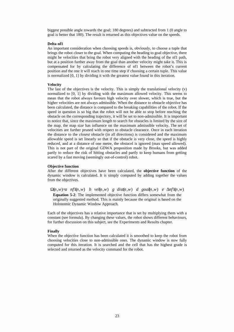
6.1. The Map Size The size of the map obviously affects the speed of computation. Not only does a bigger map fit more of the robot’s surroundings so that more obstacles are added, but also the NF1 will take longer time to compute since that is done for the whole map. Increasing the map size also influence the GDWA since it allows for higher velocities when it can plan its path further, and longer trajectories results in more check for obstacle along them. The influence that the map size and resolution has on the system is measured by moving the robot between two points in a corridor. The course does not include any obstacles in the robot’s path, but there are lots of objects on the side of the corridor that has to be inserted into the map. As mentioned above, computation time must be less than 200 ms but we would like it to be not greater than 50 ms. This test is carried out once for each setting of the map that we wish to examine. Every time that the map is recomputed the total computation time of the motion algorithm is saved onto a file. The result is showed in Table 6-1and figures Figure 6-1 to Figure 6-5.
Dimensions Mean time of computation (std deviation) [ms]
Size Res. Map NF1 GDWA Total
50 50 0.25 (0.04) 0.88 (0.03) 0.77 (0.13) 1.65 (0.14)
50 100 1.92 (0.63) 0.84 (0.25) 2.40 (0.66) 3.24 (0.76)
100 50 3.94 (1.52) 4.13 (2.42) 5.59 (4.03) 9.71 (4.91)
100 100 8.31 (4.71) 5.67 (6.56) 9.39 (5.78) 15.06 (8.86)
150 100 14.96 (12.64) 17.65 (18.26) 15.97 (13.29) 33.61 (23.34)
200 50 30.99 (29.96) 34.28 (30.00) 33.13 (31.11) 67.41 (44.43)
200 100 21.47 (20.11) 32.23 (22.78) 22.60 (20.47) 54.83 (33.33)
250 100 33.83 (27.87) 69.62 (36.51) 34.91 (27.96) 104.53 (45.43)
Table 6-1: Computation time of the system with different map configurations. The size column is actually the square root of the map size, a size of 100 means that there are 100x100 cells in the map.
Several things can be read from Table 6-1. Firstly, a larger map size obviously increases computation time. At first glance it does not seem to be a linear relationship but since a map size of 100 actually means that there are 100x100 cells in the map the computation time increases linearly with the number of cells. The next observation to be made from the table is about the resolution of the map. The resolution is the square root of the area
25
(mm2) in each cell, a resolution of 100 means that the area of each cell is 10 000 mm2. This also seems to influence the computation time but not straight forward. The natural way of arguing for how the computation time changes with the resolution is that a larger resolution results in a larger map which fit more obstacles which then takes longer time to compute. This is true for most cases but in the example above the computation time is less with the map size [200, 100] than with [200, 50]. Since the test was carried out in a corridor it is likely that all the obstacles that could be seen fit in both maps and the difference in computation time is normal variation. From the table we can also see that the standard deviation is quite large and that it increases fast with an increase in map size. This is due to two things, obstacle density and the scheduler of the operating system. The obstacle density influence the deviation with that a large map takes long time to compute when its full, when it is empty however, it does not take longer time to compute than a small. This means that the computation time for a large map varies greatly with obstacle density. Because of the long computation time, a large map is also more likely to be interrupted by the operating system than a small. Since this test is measured against a clock from start of calculation to finish, this shows in the result even if the CPU didn’t spend the whole time calculating the next velocity command.
Figure 6-1: Computation time of the motion algorithm with a map size of [50, 100] (the number of cells is 50x50 and the cells are 100x100 mm2).
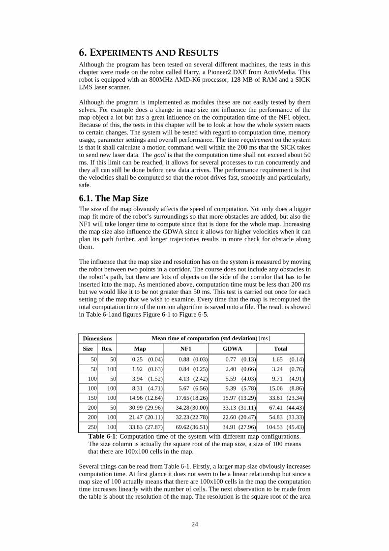
Figure 6-2: Computation with a map size of [100, 100]. The mean computation time is about 15 ms.
26
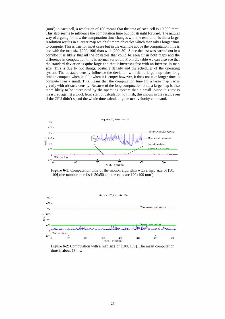
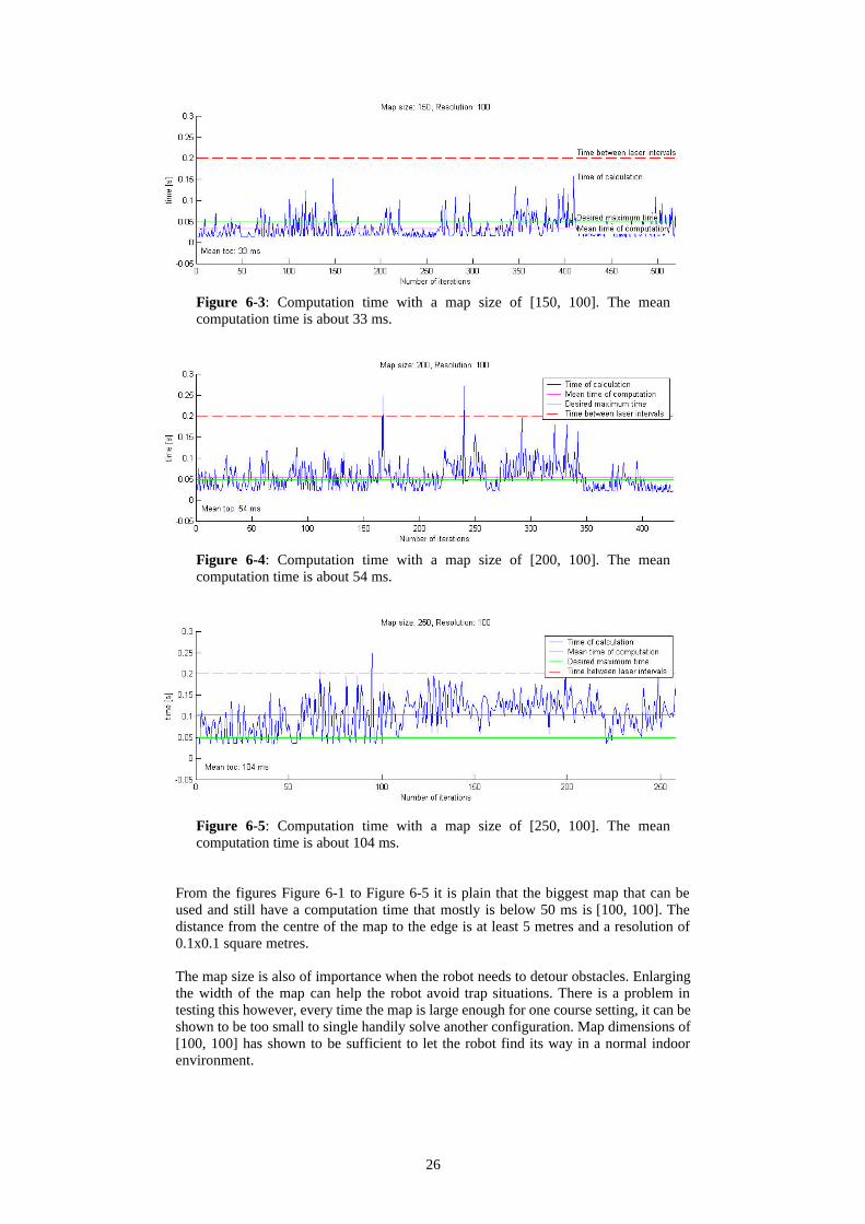
Figure 6-3: Computation time with a map size of [150, 100]. The mean computation time is about 33 ms.
Figure 6-4: Computation time with a map size of [200, 100]. The mean computation time is about 54 ms.
Figure 6-5: Computation time with a map size of [250, 100]. The mean computation time is about 104 ms.
From the figures Figure 6-1 to Figure 6-5 it is plain that the biggest map that can be used and still have a computation time that mostly is below 50 ms is [100, 100]. The distance from the centre of the map to the edge is at least 5 metres and a resolution of 0.1x0.1 square metres. The map size is also of importance when the robot needs to detour obstacles. Enlarging the width of the map can help the robot avoid trap situations. There is a problem in testing this however, every time the map is large enough for one course setting, it can be shown to be too small to single handily solve another configuration. Map dimensions of [100, 100] has shown to be sufficient to let the robot find its way in a normal indoor environment.
27
6.2. The NF1 As described earlier, the robot represents the free-space connectivity of its environment by calculating the L1 distance of every cell to the goal cell. Calculating the L1 distance is a very simple operation, despite this, to calculate the entire map of maybe 200x200 elements, a large portion of the CPU time is required. In the original proposition of the simple navigation function [18] which is the one employed in this work, NF1 is computed for the entire occupancy grid, but since the NF1 is recomputed each time new sensory data is available, this is not necessary. In Brocks solution the NF1 is only computed in a rectangular region aligned with the goal heading. If an obstacle blocks the path to the robot position the width of the region is increased until the robot’s position is reached by the wave front. This approach can save a lot of computation if the map is sufficiently large so that the extra overhead of checking whether a cell is within the rectangular region or not can be ignored. Further tests are needed to see for what sizes of the map it is justified to use this approach.
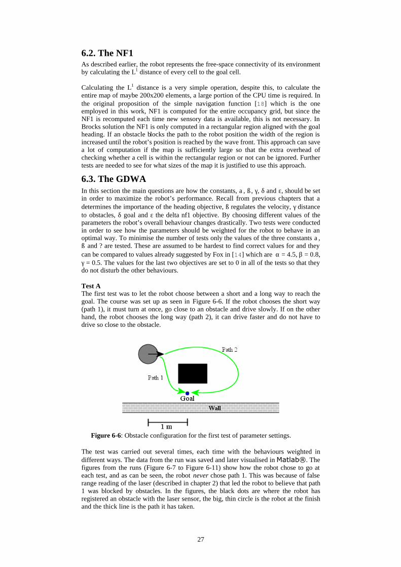
6.3. The GDWA In this section the main questions are how the constants, a , ß, γ, δ and ε, should be set in order to maximize the robot’s performance. Recall from previous chapters that a determines the importance of the heading objective, ß regulates the velocity, γ distance to obstacles, δ goal and ε the delta nf1 objective. By choosing different values of the parameters the robot’s overall behaviour changes drastically. Two tests were conducted in order to see how the parameters should be weighted for the robot to behave in an optimal way. To minimise the number of tests only the values of the three constants a , ß and ? are tested. These are assumed to be hardest to find correct values for and they can be compared to values already suggested by Fox in [14] which are α = 4.5, β = 0.8, γ = 0.5. The values for the last two objectives are set to 0 in all of the tests so that they do not disturb the other behaviours. Test A The first test was to let the robot choose between a short and a long way to reach the goal. The course was set up as seen in Figure 6-6. If the robot chooses the short way (path 1), it must turn at once, go close to an obstacle and drive slowly. If on the other hand, the robot chooses the long way (path 2), it can drive faster and do not have to drive so close to the obstacle.
Figure 6-6: Obstacle configuration for the first test of parameter settings.
The test was carried out several times, each time with the behaviours weighted in different ways. The data from the run was saved and later visualised in Matlab®. The figures from the runs (Figure 6-7 to Figure 6-11) show how the robot chose to go at each test, and as can be seen, the robot never chose path 1. This was because of false range reading of the laser (described in chapter 2) that led the robot to believe that path 1 was blocked by obstacles. In the figures, the black dots are where the robot has registered an obstacle with the laser sensor, the big, thin circle is the robot at the finish and the thick line is the path it has taken.
28
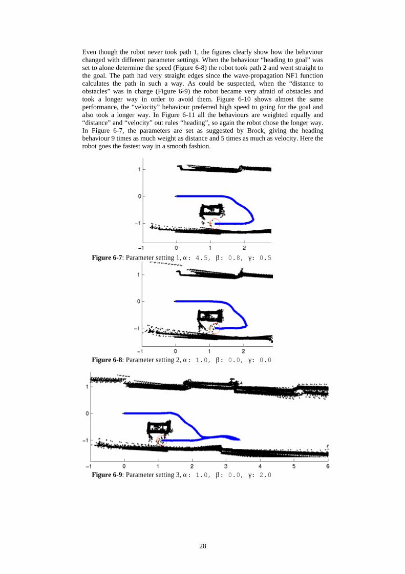
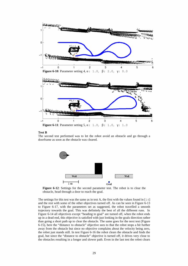
Even though the robot never took path 1, the figures clearly show how the behaviour changed with different parameter settings. When the behaviour “heading to goal” was set to alone determine the speed (Figure 6-8) the robot took path 2 and went straight to the goal. The path had very straight edges since the wave-propagation NF1 function calculates the path in such a way. As could be suspected, when the “distance to obstacles” was in charge (Figure 6-9) the robot became very afraid of obstacles and took a longer way in order to avoid them. Figure 6-10 shows almost the same performance, the “velocity” behaviour preferred high speed to going for the goal and also took a longer way. In Figure 6-11 all the behaviours are weighted equally and “distance” and “velocity” out rules “heading”, so again the robot chose the longer way. In Figure 6-7, the parameters are set as suggested by Brock, giving the heading behaviour 9 times as much weight as distance and 5 times as much as velocity. Here the robot goes the fastest way in a smooth fashion.
Figure 6-7: Parameter setting 1, α: 4.5, β: 0.8, γ: 0.5
Figure 6-8: Parameter setting 2, α: 1.0, β: 0.0, γ: 0.0
Figure 6-9: Parameter setting 3, α: 1.0, β: 0.0, γ: 2.0
29
Figure 6-10: Parameter setting 4, α: 1.0, β: 2.0, γ: 0.0
Figure 6-11: Parameter setting 5, α: 1.0, β: 1.0, γ: 1.0
Test B The second test performed was to let the robot avoid an obstacle and go through a doorframe as soon as the obstacle was cleared.
Figure 6-12: Settings for the second parameter test. The robot is to clear the obstacle, head through a door to reach the goal.
The settings for this test was the same as in test A, the first with the values found in [14] and the rest with some of the other objectives turned off. As can be seen in Figure 6-13 to Figure 6-17, with the parameters set as suggested, the robot travelled a smooth trajectory towards the goal. This was definitely the best of all the different runs. In Figure 6-14 all objectives except “heading to goal” are turned off, when the robot ends up in a dead end, this objective is satisfied with just looking in the goals direction rather than going a short path up to clear the obstacle. The same goes for the next test (Figure 6-15), here the “distance to obstacle” objective sees to that the robot stops a bit further away from the obstacle but since no objective complains about the velocity being zero, the robot just stands still. In test Figure 6-16 the robot clears the obstacle and finds the goal, but since the “distance to obstacle” objective is turned off, it drives very close to the obstacles resulting in a longer and slower path. Even in the last test the robot clears
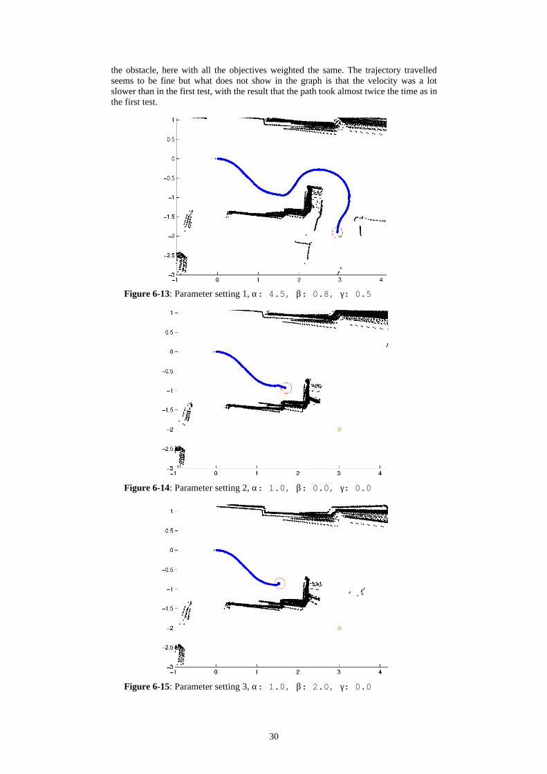
30
the obstacle, here with all the objectives weighted the same. The trajectory travelled seems to be fine but what does not show in the graph is that the velocity was a lot slower than in the first test, with the result that the path took almost twice the time as in the first test.
Figure 6-13: Parameter setting 1, α: 4.5, β: 0.8, γ: 0.5
Figure 6-14: Parameter setting 2, α: 1.0, β: 0.0, γ: 0.0
Figure 6-15: Parameter setting 3, α: 1.0, β: 2.0, γ: 0.0
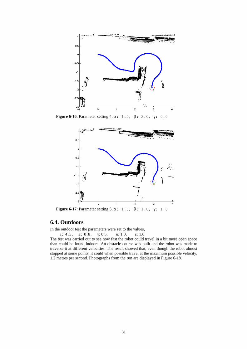
31
Figure 6-16: Parameter setting 4, α: 1.0, β: 2.0, γ: 0.0
Figure 6-17: Parameter setting 5, α: 1.0, β: 1.0, γ: 1.0
6.4. Outdoors In the outdoor test the parameters were set to the values,
a : 4 .5, ß : 0 .8, γ: 0.5, δ: 1.0, ε: 1.0 The test was carried out to see how fast the robot could travel in a bit more open space than could be found indoors. An obstacle course was built and the robot was made to traverse it at different velocities. The result showed that, even though the robot almost stopped at some points, it could when possible travel at the maximum possible velocity, 1.2 metres per second. Photographs from the run are displayed in Figure 6-18.
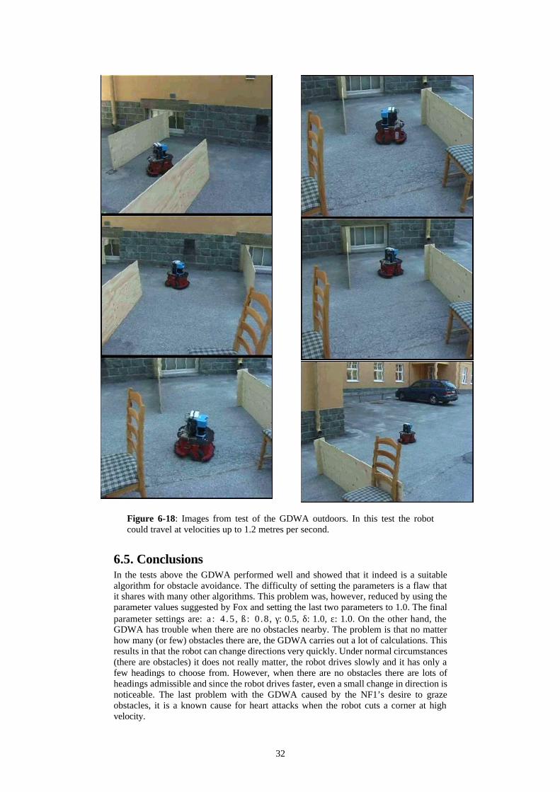
32
Figure 6-18: Images from test of the GDWA outdoors. In this test the robot could travel at velocities up to 1.2 metres per second.
6.5. Conclusions In the tests above the GDWA performed well and showed that it indeed is a suitable algorithm for obstacle avoidance. The difficulty of setting the parameters is a flaw that it shares with many other algorithms. This problem was, however, reduced by using the parameter values suggested by Fox and setting the last two parameters to 1.0. The final parameter settings are: a : 4 .5, ß : 0 .8, γ: 0.5, δ: 1.0, ε: 1.0. On the other hand, the GDWA has trouble when there are no obstacles nearby. The problem is that no matter how many (or few) obstacles there are, the GDWA carries out a lot of calculations. This results in that the robot can change directions very quickly. Under normal circumstances (there are obstacles) it does not really matter, the robot drives slowly and it has only a few headings to choose from. However, when there are no obstacles there are lots of headings admissible and since the robot drives faster, even a small change in direction is noticeable. The last problem with the GDWA caused by the NF1’s desire to graze obstacles, it is a known cause for heart attacks when the robot cuts a corner at high velocity.
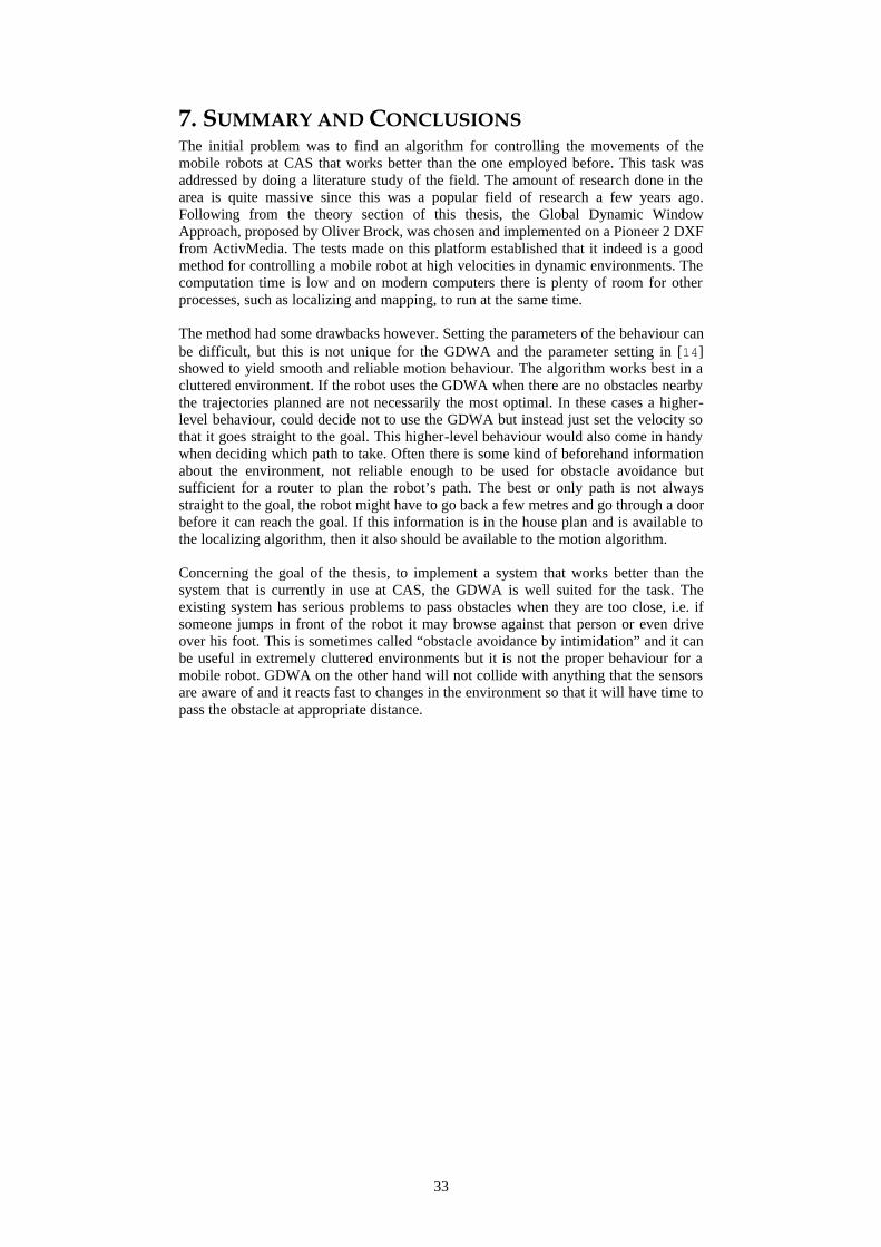
33
7. SUMMARY AND CONCLUSIONS The initial problem was to find an algorithm for controlling the movements of the mobile robots at CAS that works better than the one employed before. This task was addressed by doing a literature study of the field. The amount of research done in the area is quite massive since this was a popular field of research a few years ago. Following from the theory section of this thesis, the Global Dynamic Window Approach, proposed by Oliver Brock, was chosen and implemented on a Pioneer 2 DXF from ActivMedia. The tests made on this platform established that it indeed is a good method for controlling a mobile robot at high velocities in dynamic environments. The computation time is low and on modern computers there is plenty of room for other processes, such as localizing and mapping, to run at the same time. The method had some drawbacks however. Setting the parameters of the behaviour can be difficult, but this is not unique for the GDWA and the parameter setting in [14] showed to yield smooth and reliable motion behaviour. The algorithm works best in a cluttered environment. If the robot uses the GDWA when there are no obstacles nearby the trajectories planned are not necessarily the most optimal. In these cases a higher-level behaviour, could decide not to use the GDWA but instead just set the velocity so that it goes straight to the goal. This higher-level behaviour would also come in handy when deciding which path to take. Often there is some kind of beforehand information about the environment, not reliable enough to be used for obstacle avoidance but sufficient for a router to plan the robot’s path. The best or only path is not always straight to the goal, the robot might have to go back a few metres and go through a door before it can reach the goal. If this information is in the house plan and is available to the localizing algorithm, then it also should be available to the motion algorithm. Concerning the goal of the thesis, to implement a system that works better than the system that is currently in use at CAS, the GDWA is well suited for the task. The existing system has serious problems to pass obstacles when they are too close, i.e. if someone jumps in front of the robot it may browse against that person or even drive over his foot. This is sometimes called “obstacle avoidance by intimidation” and it can be useful in extremely cluttered environments but it is not the proper behaviour for a mobile robot. GDWA on the other hand will not collide with anything that the sensors are aware of and it reacts fast to changes in the environment so that it will have time to pass the obstacle at appropriate distance.
34
8. FUTURE WORK As described in the previous section, the GDWA should not work alone. The best result will be obtained if the GDWA is merely one behaviour among other and the planning is done at a higher instance. This higher instance will never call the GDWA in situations where another behaviour would perform better, for example when there are no obstacles to avoid. This planner, or router, would also divide the path into several small steps that it hands out to the GDWA one at a time. In this way it might avoid most of the trap situations that the robot can get caught in. One disadvantage with the implementation described in this work is that it assumes that the robot is circular. This greatly simplifies calculations but it has the obvious drawback that a robot shaped differently has to be considered a circle with a radius that is equal to the longest distance from the robot centre to the edge. This result in that the robot will require more space in the map than it does in the real world which in turn result in that the motion behaviour will not allow the robot to drive as close to obstacles as it really could. A possible way of solving this in a future implementation is to consider the robot as a polygon and using fixed look-up tables. One method based on the GDWA that does not use look-up tables is discussed in [3]. The NF1’s inherent enthusiasm for selecting the shortest route when passing an obstacle could be lessened by adding side clearance to the objective function. Searching the robot’s trajectory for this as well as distance to obstacle would greatly increase computation time, but even here the use of lookup tables could be employed.
35
REFERENCES [1] M. Andersson, A. Orebäck, M. Lindström, and H. I. Christensen. “ISR: An intelligent
service robot.” In H. I. Christensen, H. Bunke, and H. Noltmeier, editors, Intelligent Sensor Based Robotics, pages 287-310. Springer, Berlin, 1999.
[2] Arkin, Ronald C, “Behavior-Based Robotics”, the MIT Press, 1998. [3] Kai O. Arras, et al, “Real-Time Obstacle Avoidance For Polygonal Robots With A
Reduced Dynamic Window”, in proc. IEEE Int. Conf on Robotics and Automation, Washington, DC, May 2002
[4] R. Bauer, W. Feiten and G. Lawitzky, “Steer Angle Fields: An Approach to Robust Manoeuvring in Cluttered, Unknown Environments”, In Proc. Int. Workshop on Intelligent Robotic Systems, Zakopane, July 1993.
[5] J. Borenstein and Y. Koren, “Real-time Obstacle Avoidance for Fast Mobile Robots.” IEEE Trans. on Systems, Man, and Cybernetics, Vol. 19, No. 5, Sept./Oct. 1989, p 1179-1187.
[6] J. Borenstein and Y. Koren, “The Vector Field Histogram – Fast Obstacle Avoidance for Mobile Robots”, IEEE Journal of Robotics and Automation, Vol. 7, No 3, June 1991, p 278-288.
[7] J.Borenstein and Y.Koren. Histogramic In-Motion Mapping for Mobile Robot Obstacle Avoidance. IEEE Trans. on Robot. and Automation, Vol. 7, No 4, Aug 1991, p 535-539.
[8] O. Brock, “Generating Robot Motion: The Integration of Planning and Execution”, Doctoral Thesis, Stanford University, 1999.
[9] O. Brock and O. Khatib, “High-Speed Navigation Using the Global Dynamic Window Approach”, in Proc. IEEE Int. Conf. on Robotics and Automation, Detroit, USA, May 1999.
[10] E. Coste-Maniére and R. Simmons, “Architecture, the Backbone of Robotic Systems”, in Proc IEEE Int. Conf. on Robotics and Automation, April 2000.
[11] A. Elfes, “Sonar-Based Real-World Mapping and Navigation”, IEEE Journal on Robotics and Automation, Vol. 3, No. 3, June 1987, p 249-265
[12] H. Everett, “Sensors for Mobile Robots: Theory and Application”, AK Peters, Ltd., 1995. [13] D. Fox, W. Burgard and S. Thrun, “Controlling Synchro-Drive Robots with the Dynamic
Window Approach to Collision Avoidance”, in Proc. IROS, 1996. [14] D. Fox, “Markov Localization: A Probabilistic Framework for Mobile Robot Localization
and Navigation”, Doctoral Thesis, University of Bonn, 1998. [15] D. Hogg, F. Martin and R. Resnick, “Braienberg Creatures”, Epistemology and Learning
Memo 13, MIT Media lab, 1991. [16] Suk hyung Jung, et al, “Local Obstacle Avoidance for Synchro-Drive Mobile Robot”, IEEE
Tencon, 1999. [17] Y. Koren and J. Borenstein, “Analysis of Control Methods for Mobile Robot Obstacle
Avoidance”, in Proc. IEEE Int. Workshop Intelligent Motion Control, 1990. [18] Jean-Claude Latombe, “Robot Motion Planning”, Kluwer Academic Publishers, Boston,
1991 [19] H. Moravec and A.E. Elfes, “High Resolution Maps from Wide Angle Sonar”, in Proc.
IEEE Int. Conf. on Robotics and Automation, March, 1985 [20] R. Simmons, “The Curvature-Velocity Method for Local Obstacle Avoidance”, in Proc.
Int. Conf. On Robotics and Automation, Minneapolis, April 1996. [21] I. Ulrich and J. Borenstein, “VFH+: Reliable Obstacle Avoidance for Fast Mobile
Robots”, in Proc. IEEE Int. Conf. on Robotics and Automation, Leuven, Belgium, May 1998.
[22] O. Wijk, “Triangulation Based Fusion of Sonar Data with Application in Mobile Robot Mapping and Localisation”, Doctoral Thesis, Department of Signals, Sensors and Systems, Royal Institute of Technology (KTH), Stockholm, Sweden, 2001.
[23] Web page of the Centre of Autonomous Systems, www.nada.kth.se/cas, September 2002.
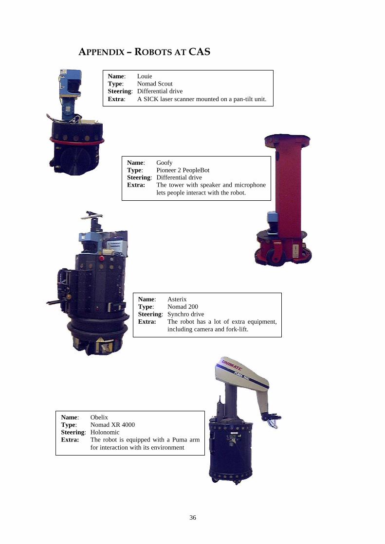
36
APPENDIX – ROBOTS AT CAS
Name: Louie Type: Nomad Scout Steering: Differential drive Extra: A SICK laser scanner mounted on a pan-tilt unit.
Name: Goofy Type: Pioneer 2 PeopleBot Steering: Differential drive Extra: The tower with speaker and microphone
lets people interact with the robot.
Name: Asterix Type: Nomad 200 Steering: Synchro drive Extra: The robot has a lot of extra equipment,
including camera and fork-lift.
Name: Obelix Type: Nomad XR 4000 Steering: Holonomic Extra: The robot is equipped with a Puma arm
for interaction with its environment