obstacle avoidance for unmanned air vehicles using ...beard/papers/thesis/brandoncall.pdf ·...
TRANSCRIPT
OBSTACLE AVOIDANCE FOR UNMANNED AIR VEHICLES
by
Brandon R. Call
A thesis submitted to the faculty of
Brigham Young University
in partial fulfillment of the requirements for the degree of
Master of Science
Electrical and Computer Engineering
Brigham Young University
December 2006


Copyright c© 2006 Brandon R. Call
All Rights Reserved


BRIGHAM YOUNG UNIVERSITY
GRADUATE COMMITTEE APPROVAL
of a thesis submitted by
Brandon R. Call
This thesis has been read by each member of the following graduate committee andby majority vote has been found to be satisfactory.
Date Randal W. Beard, Chair
Date Clark N. Taylor
Date James K. Archibald

BRIGHAM YOUNG UNIVERSITY
As chair of the candidate’s graduate committee, I have read the thesis of Brandon R.Call in its final form and have found that (1) its format, citations, and bibliograph-ical style are consistent and acceptable and fulfill university and department stylerequirements; (2) its illustrative materials including figures, tables, and charts are inplace; and (3) the final manuscript is satisfactory to the graduate committee and isready for submission to the university library.
Date Randal W. BeardChair, Graduate Committee
Accepted for the Department
Michael J. WirthlinGraduate Coordinator
Accepted for the College
Alan R. ParkinsonDean, Ira A. Fulton College ofEngineering and Technology

ABSTRACT
OBSTACLE AVOIDANCE FOR UNMANNED AIR VEHICLES
Brandon R. Call
Electrical and Computer Engineering
Master of Science
Small UAVs are used for low altitude surveillance flights where unknown ob-
stacles can be encountered. These UAVs can be given the capability to navigate in
uncertain environments if obstacles are identified. This research presents an obstacle
avoidance system for small UAVs. First, a mission waypoint path is created that
avoids all known obstacles using a genetic algorithm. Then, while the UAV is in
flight, obstacles are detected using a forward looking, onboard camera. Image fea-
tures are found using the Harris Corner Detector and tracked through multiple video
frames which provides three dimensional localization of the features. A sparse three
dimensional map of features provides a rough estimate of obstacle locations. The
features are grouped into potentially hazardous areas. The small UAV then employs
a sliding mode control law on the autopilot to avoid obstacles.


This research compares rapidly-exploring random trees to genetic algorithms
for UAV pre-mission path planning. It also presents two methods for using image
feature movement and UAV telemetry to calculate depth and detect obstacles. The
first method uses pixel ray intersection and the second calculates depth from image
feature movement. Obstacles are avoided with a success rate of 99.2%.


ACKNOWLEDGMENTS
I would like to thank my professors Randy Beard, Clark Taylor, Tim McLain
and James Archibald for providing an environment where I could succeed and for
giving me guidance and inspiration. I would like to thank AFOSR for financially
supporting my research with grant number FA9550-04-C-0032. Additionally, I thank
Robert Murphy, Kevin O’Neal, David Jeffcoat and Will Curtis at the Munitions
Directorate of the Air Force Research Laboratory at Eglin Air Force Base where I
completed some of this research and had an enjoyable learning experience as a summer
intern. I would also like to thank MIT Lincoln Laboratory for providing me funding
in the form of a Graduate Research Fellowship.
I would like to thank the students of the MAGICC lab for helping me get
through classes and for providing an atmosphere where good ideas can be carried
through to experimentation. Thanks to Nate Knoebal and Joe Jackson for helping
me get a UAV in the air long enough to get some data.
Lastly, I would like to thank my supportive wife, Emily, for putting in some
hard work of her own. She always encourages me to be the best that I can be. She
helped me see the light at the end of the tunnel when it was dim.

Table of Contents
Acknowledgements xiii
List of Tables xix
List of Figures xxii
1 Introduction 1
1.1 UAV Applications . . . . . . . . . . . . . . . . . . . . . . . . . . . . . 1
1.2 Pre-Mission Path Planning . . . . . . . . . . . . . . . . . . . . . . . . 2
1.3 Reactive Path Planning . . . . . . . . . . . . . . . . . . . . . . . . . 4
1.4 Obstacle Avoidance for Small UAVs . . . . . . . . . . . . . . . . . . . 5
2 Pre-Mission Path Planning 7
2.1 Rapidly-Exploring Random Trees . . . . . . . . . . . . . . . . . . . . 8
2.1.1 RRT Algorithm Description . . . . . . . . . . . . . . . . . . . 8
2.1.2 RRT Results . . . . . . . . . . . . . . . . . . . . . . . . . . . 9
2.2 Genetic Algorithm . . . . . . . . . . . . . . . . . . . . . . . . . . . . 11
2.2.1 Genetic Algorithm Description . . . . . . . . . . . . . . . . . . 11
2.2.2 Genetic Algorithm Results . . . . . . . . . . . . . . . . . . . . 15
2.3 Path Planner Comparison . . . . . . . . . . . . . . . . . . . . . . . . 16
3 Feature Tracking 21
3.1 Feature Detection . . . . . . . . . . . . . . . . . . . . . . . . . . . . . 22
xv
3.1.1 Measuring Pixel Information . . . . . . . . . . . . . . . . . . . 22
3.1.2 Harris Corner Detector . . . . . . . . . . . . . . . . . . . . . . 23
3.2 Feature Selection . . . . . . . . . . . . . . . . . . . . . . . . . . . . . 24
3.3 Image Correlation . . . . . . . . . . . . . . . . . . . . . . . . . . . . . 25
3.4 Feature Tracking for Obstacle Avoidance . . . . . . . . . . . . . . . . 26
3.4.1 Window size and frequency of tracking . . . . . . . . . . . . . 26
3.5 Conclusion . . . . . . . . . . . . . . . . . . . . . . . . . . . . . . . . . 28
4 Obstacle Detection 31
4.1 Preliminaries . . . . . . . . . . . . . . . . . . . . . . . . . . . . . . . 31
4.2 Obstacle Detection Using Three Dimensional Ray Intersection . . . . 34
4.2.1 Three Dimensional Ray Intersection . . . . . . . . . . . . . . . 35
4.2.2 Feature Clustering . . . . . . . . . . . . . . . . . . . . . . . . 36
4.2.3 The Ill Conditioned Nature of This Problem . . . . . . . . . . 37
4.3 Obstacle Detection Using Depth From Motion . . . . . . . . . . . . . 39
4.3.1 Calculating Depth From Motion . . . . . . . . . . . . . . . . . 39
4.3.2 Handling Obstacles of Multiple Depths . . . . . . . . . . . . . 41
4.3.3 Analysis of the Depth from Motion Obstacle Detection Method 43
4.4 Conclusion . . . . . . . . . . . . . . . . . . . . . . . . . . . . . . . . . 44
5 Obstacle Avoidance 47
5.1 Sliding Mode Orbit Controller . . . . . . . . . . . . . . . . . . . . . . 47
5.2 Using the Orbit Controller . . . . . . . . . . . . . . . . . . . . . . . . 49
5.3 Alternative Obstacle Avoidance Controllers . . . . . . . . . . . . . . . 50
5.4 Conclusion . . . . . . . . . . . . . . . . . . . . . . . . . . . . . . . . . 52
6 Experimental Architecture 53
xvi
6.1 Simulation . . . . . . . . . . . . . . . . . . . . . . . . . . . . . . . . . 53
6.2 Hardware . . . . . . . . . . . . . . . . . . . . . . . . . . . . . . . . . 55
7 Flight Experiments 57
7.1 Obstacle Avoidance in Simulation . . . . . . . . . . . . . . . . . . . . 57
7.1.1 Single Obstacle . . . . . . . . . . . . . . . . . . . . . . . . . . 58
7.1.2 Multiple Obstacles . . . . . . . . . . . . . . . . . . . . . . . . 60
7.1.3 Angled Obstacle . . . . . . . . . . . . . . . . . . . . . . . . . 62
7.1.4 Obstacle Avoidance Controller . . . . . . . . . . . . . . . . . . 64
7.1.5 Comparison . . . . . . . . . . . . . . . . . . . . . . . . . . . . 66
7.2 Obstacle Avoidance on UAV Hardware . . . . . . . . . . . . . . . . . 67
7.3 Summary . . . . . . . . . . . . . . . . . . . . . . . . . . . . . . . . . 69
8 Conclusion 71
8.1 Future Work . . . . . . . . . . . . . . . . . . . . . . . . . . . . . . . . 72
Bibliography 77
A Random City Maker 79
A.1 Introduction . . . . . . . . . . . . . . . . . . . . . . . . . . . . . . . . 79
A.2 How to Create and Use Cities . . . . . . . . . . . . . . . . . . . . . . 80
A.2.1 The Random City Maker User Interface . . . . . . . . . . . . 80
A.2.2 Create a City . . . . . . . . . . . . . . . . . . . . . . . . . . . 82
A.3 Using City Files for Research Testing . . . . . . . . . . . . . . . . . . 83
A.3.1 How to Use Cities in Aviones . . . . . . . . . . . . . . . . . . 83
A.3.2 How to Use Cities in the Path Planner . . . . . . . . . . . . . 84
A.4 City Generation Algorithm and Implementation . . . . . . . . . . . . 84
A.4.1 Internal C++ Classes . . . . . . . . . . . . . . . . . . . . . . . 85
xvii
A.4.2 City Generation Algorithm . . . . . . . . . . . . . . . . . . . . 86
A.4.3 Height Functions . . . . . . . . . . . . . . . . . . . . . . . . . 88
A.5 Conclusion . . . . . . . . . . . . . . . . . . . . . . . . . . . . . . . . . 89
A.5.1 Future Work . . . . . . . . . . . . . . . . . . . . . . . . . . . . 90
xviii
List of Tables
2.1 RRT Parameter Values . . . . . . . . . . . . . . . . . . . . . . . . . . 11
2.2 Genetic Algorithm Parameters Values . . . . . . . . . . . . . . . . . . 16
2.3 Path Planner Comparison Results . . . . . . . . . . . . . . . . . . . . 18
2.4 Path Planning Algorithm Trade-offs . . . . . . . . . . . . . . . . . . . 19
7.1 Monte Carlo Simulation Results . . . . . . . . . . . . . . . . . . . . . 66
7.2 Simulation vs. Hardware . . . . . . . . . . . . . . . . . . . . . . . . . 67
7.3 Source of Hardware Error . . . . . . . . . . . . . . . . . . . . . . . . 68
A.1 City Maker Height Function Parameter Values . . . . . . . . . . . . . 82
xix

xx
List of Figures
1.1 A Small, Fixed-Wing UAV . . . . . . . . . . . . . . . . . . . . . . . . 2
2.1 Rapidly-Exploring Random Tree Diagram . . . . . . . . . . . . . . . 9
2.2 Rapidly-Exploring Random Tree Example . . . . . . . . . . . . . . . 10
2.3 Genetic Algorithm Initial Population Diagram . . . . . . . . . . . . . 13
2.4 Genetic Algorithm Sensitivity to Initial Number of Waypoints . . . . 17
2.5 Genetic Algorithm Path Planning Example . . . . . . . . . . . . . . . 18
3.1 Corners as Image Features . . . . . . . . . . . . . . . . . . . . . . . . 23
3.2 Image Correlation Window Size . . . . . . . . . . . . . . . . . . . . . 27
3.3 Feature Movement vs. Time Between Telemetry Packets . . . . . . . 29
4.1 Ray-Circle Intersection . . . . . . . . . . . . . . . . . . . . . . . . . . 33
4.2 Obstacle Localization Using Ray Intersection . . . . . . . . . . . . . . 35
4.3 Telemetry Packet Update Time vs. Percentage of Features Tracked . 38
4.4 Ray Intersection Sensitivity to Heading Estimate Error . . . . . . . . 39
4.5 Depth Calculation Sensitivity to Objects at Multiple Depths . . . . . 42
4.6 A Comparison of Two-Feature Depth vs Epipole Depth . . . . . . . . 45
5.1 Vector Field Used To Fly an Orbit . . . . . . . . . . . . . . . . . . . 48
5.2 The Ideal Detection of an Obstacle . . . . . . . . . . . . . . . . . . . 49
5.3 UAV Avoiding an Obstacle With Depth . . . . . . . . . . . . . . . . 50
5.4 Controller Simulation . . . . . . . . . . . . . . . . . . . . . . . . . . . 51
xxi
6.1 The UAV System . . . . . . . . . . . . . . . . . . . . . . . . . . . . . 54
6.2 UAV test hardware . . . . . . . . . . . . . . . . . . . . . . . . . . . . 55
6.3 Kestrel Autopilot . . . . . . . . . . . . . . . . . . . . . . . . . . . . . 56
7.1 Simulation Results - Height Estimations . . . . . . . . . . . . . . . . 58
7.2 One Obstacle Simulator Screen Capture . . . . . . . . . . . . . . . . 59
7.3 Simulation Results - One Obstacle . . . . . . . . . . . . . . . . . . . . 60
7.4 Simulation Results - One Obstacle Overhead Perspective . . . . . . . 61
7.5 Two Obstacle Environment Screen Capture . . . . . . . . . . . . . . 61
7.6 Simulation Results - Two Obstacles Scatter Plot . . . . . . . . . . . . 62
7.7 Simulation Results - Two Obstacles Overhead Perspective . . . . . . 63
7.8 One Rotated Obstacle Screen Capture . . . . . . . . . . . . . . . . . 63
7.9 Simulation Results - Rotated Building Scatter . . . . . . . . . . . . . 64
7.10 Simulation Results - Rotated Building Overhead . . . . . . . . . . . . 65
7.11 Simulation Results - UAV Flight Path . . . . . . . . . . . . . . . . . 66
A.1 Random City Maker Screen Shot . . . . . . . . . . . . . . . . . . . . 81
A.2 A City in the Aviones Simulator . . . . . . . . . . . . . . . . . . . . . 84
A.3 City Generation Algorithm Diagram . . . . . . . . . . . . . . . . . . 87
A.4 Three City Height Function Examples . . . . . . . . . . . . . . . . . 91
A.5 Graphs of Height Functions . . . . . . . . . . . . . . . . . . . . . . . 92
xxii
Chapter 1
Introduction
1.1 UAV Applications
The tasks of following a wanted suspect, monitoring the growth of a forest fire
and exploring areas with hazardous airborne chemicals have one thing in common:
they are jobs that a small unmanned air vehicle could do. UAVs have the potential
of being employed to make humans more productive or to do new tasks that are
too dangerous or impossible for unaided humans. UAV research has been heavily
funded by the United States Department of Defense because UAVs save the lives of
soldiers and provide new capabilities to ground and air troops. When used for mil-
itary applications, UAVs can provide convoy surveillance, target localization, target
prosecution, communications transmissions and even border and port surveillance.
Additionally, UAVs are viable solutions for civil and commercial applications.
UAVs can be used for monitoring critical infrastructure, real-time disaster observance,
wilderness search and rescue and in-storm weather measurements. UAVs may poten-
tially be used as a low-cost solution where manned helicopters are currently employed
including traffic monitoring, obtaining a birds-eye view of a major sporting or news
event, estimating the movement of forest fires, tracking high-speed chases, following
criminals on the run or monitoring the movements of city protests.
Many of these applications for small UAVs require the ability to navigate in
urban or unknown terrain where many obstacles of different types and sizes may
endanger the safety of the mission. UAVs must have the ability to autonomously
plan trajectories that are free from collision with buildings, trees or unlevel ground
or other obstacles in order to be effective. Furthermore, for higher flying missions
where obstacles are not expected, any UAV that enters commercial airspace must
1
meet strict requirements established by the Federal Aviation Administration (FAA).
One of these requirements is that the UAV must be able to see and avoid potential
hazards. These requirements can be addressed by using pre-mission path planning
in conjunction with a reactive path planning system. This research addresses both
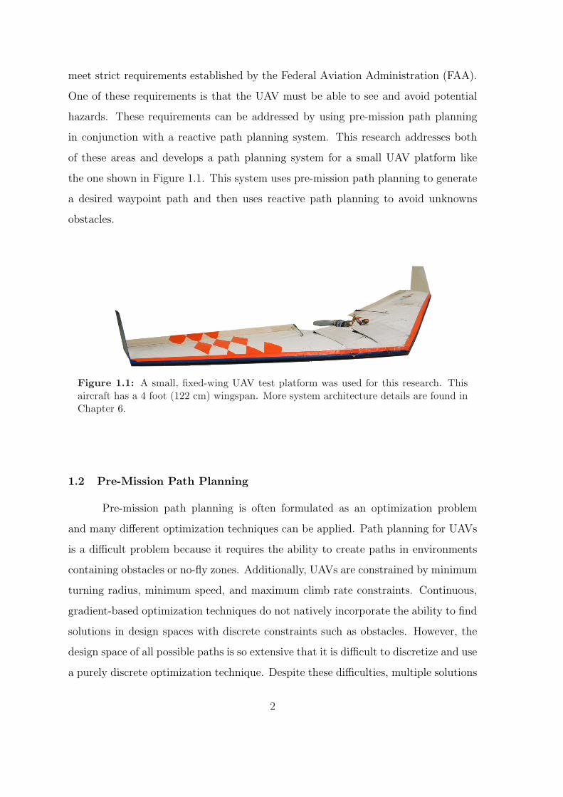
of these areas and develops a path planning system for a small UAV platform like
the one shown in Figure 1.1. This system uses pre-mission path planning to generate
a desired waypoint path and then uses reactive path planning to avoid unknowns
obstacles.
Figure 1.1: A small, fixed-wing UAV test platform was used for this research. Thisaircraft has a 4 foot (122 cm) wingspan. More system architecture details are found inChapter 6.
1.2 Pre-Mission Path Planning
Pre-mission path planning is often formulated as an optimization problem
and many different optimization techniques can be applied. Path planning for UAVs
is a difficult problem because it requires the ability to create paths in environments
containing obstacles or no-fly zones. Additionally, UAVs are constrained by minimum
turning radius, minimum speed, and maximum climb rate constraints. Continuous,
gradient-based optimization techniques do not natively incorporate the ability to find
solutions in design spaces with discrete constraints such as obstacles. However, the
design space of all possible paths is so extensive that it is difficult to discretize and use
a purely discrete optimization technique. Despite these difficulties, multiple solutions
2
have been proposed. Generally, random algorithms are used to sparsely search the
space for solutions and then the best solution is chosen.
Many different methods have been used for robot path planning. Ref. [1] uses
mixed integer linear programming (MILP) to plan paths for UAVs and other vehicles
with turning constraints and minimum speed requirements. They assume a receding
horizon of knowledge about the environment and plan paths that ensure the vehicle
can reach a safe basis state and remain there for an indefinite amount of time.
Ref. [2] presents a method for aiding a path planner to create paths that
navigate narrow passages. Random lines of a fixed length are created and compared
with a map of the environment. Lines with endpoints that are inside obstacles and
midpoints that are outside obstacles are stored. The midpoints of all lines are then
connected in a feasibility graph which a path planner can then search for a low-cost
path.
A discretized three-dimensional model is used in [3] built on research in [4] to
plan paths for autonomous helicopters. The model has a hierarchical discretization
and employs standard Dijkstra or A* graph search to find an optimal solution at each
hierarchy level. They refine their three-dimensional model using computer vision 3D
reconstruction. This work is similar to the work presented in this thesis, however
this research finds good results without performing computationally expensive 3D
reconstruction and without storing a large, multi-resolution terrain map so that paths
can be planned for small UAVs with limited resources.
This research also employs a genetic or evolutionary algorithm for UAV path
planning which is similar to the evolutionary approach in [5]. However, the target
platform used in [5] is a weather tracking UAV which encounters only a handful of
obstacles at one time. This thesis, however, targets low-flying, small UAVs operating
in urban terrain and consequently formulates the genetic algorithm quite differently
and evaluates the algorithm for environments with numerous obstacles.
Bortoff [6] refines a Voronoi graph path planning algorithm to avoid radar
detection for UAVs. This method is useful for two dimensional path planning where
obstacles are represented by points in space, but the Voronoi graph method is difficult
3
to implement in a three-dimensional environment with obstacles that are larger than
single points.
1.3 Reactive Path Planning
Reactive path planning is a two step process, sensing the obstacles in the
environment and then controlling the vehicle around detected obstacles. Sensing the
environment may be done in a variety of ways including laser range finders, optical
flow sensors, stereo camera pairs or a moving single camera. There are also multiple
ways to control the vehicle in the presence of obstacles, including steering potential
functions and a sliding mode controller.
Laser range finders are commonly used to detect obstacles and are effective if
they can be scanned or pivoted. However, scanning hardware is too large and heavy
for small UAVs. Saunders [7] made use of a single, fixed laser range finder, but its
capabilities to detect the environment were limited.
Alternately, video cameras are light and inexpensive and thereby fit the phys-
ical requirements of the small UAVs. Video cameras can be configured for obstacle
detection as a stereo pair, or a moving single camera. Sabe [8] describes how to use a
stereo camera pair to make planar approximations of the environment, and Badal [9]
employs stereo matching using image disparity to navigate a ground vehicle.
Video cameras, however, provide information in a way that requires significant
data processing to be useful for autonomous control. One method is to reconstruct
the three-dimensional environment and use a global path planner as discussed above.
ref. [10] contains a survey of three-dimensional reconstruction. Three-dimensional
reconstruction, however requires more processing power than can be found on-board
a small UAV or on a small mobile ground station and is therefore difficult to implement
for small UAVs. Less demanding algorithms have been used for small ground robots
and have been found suitable.
In research similar to the work presented here, ref [11] used image feature flow
to drive a ground robot navigating a hallway. ref [11] assumes a structured indoor
environment and also allows the robot to stop, turn and then proceed. Huber [12]
4

explains how to calculate distance and depth from motion without camera calibration.
This method is implemented for an industrial ground vehicle.
Despite the excellent research performed in the areas of path planning and
computer vision, a path planner using a passive sensor such as a video camera that
can sense and avoid obstacles in real-time has not been successfully implemented for
a small UAV platform.
1.4 Obstacle Avoidance for Small UAVs
This research develops a path planning system with real-time obstacle avoid-
ance using a single video camera for a small UAV platform. Both pre-mission path
planning and in-flight, reactive path planning are employed for the safe navigation of
the UAV’s mission. The system is required to operate fast enough to enable the UAV
to react in real-time to its environment and must also be light enough to be flown on
a small UAV. Additionally, this research requires the use of a mobile ground station
to be useful for military applications which implies computation must be done on a
laptop.
This thesis begins with a discussion of pre-mission path planning in Chap-
ter 2. A rapidly-exploring random tree implementation is compared with a genetic
algorithm implementation. Chapter 3 through Chapter 5 describe the reactive path
planning system. Chapter 3 begins with details about the computer vision algorithms
for tracking image features and the implications for a path planning system. Then
in Chapter 4, two methods for using image features and the telemetry of the UAV to
detect and localize obstacles are presented. The two methods are implemented and
evaluated for reactive path planning. Chapter 5 presents a sliding mode control law
that can be used to avoid obstacles. Chapter 6 explains both the hardware and the
software architecture of the UAV system including a simulation environment. Results
from software simulations and hardware demonstrations are provided in Chapter 7
along with an analysis of the effectiveness of the system. The conclusion includes
lessons learned and future improvements to the obstacle avoidance system and other
interesting research topics for future work in the area of UAV path planning. Addi-
5

tionally, Appendix A gives details about the Random City Maker that was developed
to facilitate path planning and computer vision testing for UAVs.
6
Chapter 2
Pre-Mission Path Planning
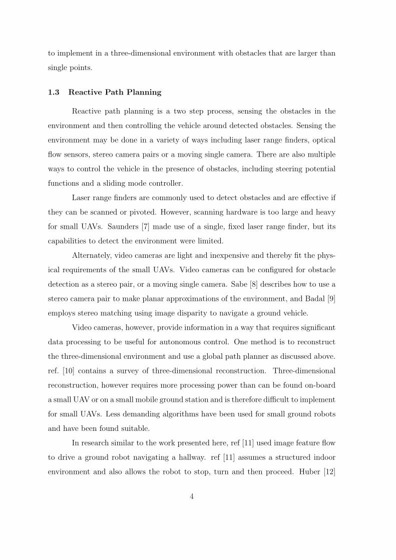
Small UAVs can potentially be used for urban surveillance, convoy protection,
forest fire tracking and wilderness search and rescue. Each of these applications
requires the UAV to plan a flight path to accomplish some objective. The flight
path must be flyable and the UAV must not collide with any known obstacles. In
this work, known obstacles are represented using an elevation map because maps
are readily available from the United States Geological Survey website. Ideally, the
obstacle set is represented by a list of objects defined by polygonal boundaries so that
path intersections can be determined easily. However, all terrain data is available in
elevation grid format which requires incremental path checking. The path planning
task is to use a the given elevation map to generate a waypoint path starting at the
UAV’s current state and ending at the UAV’s goal state.
Multiple algorithms have been applied to path planning for robots in the pres-
ence of known obstacles. Some of these algorithms are potential fields [13], Voronoi
graphs [6], visibility graphs, rapidly-exploring random trees (RRT) [14] and genetic
algorithms [5]. Voronoi graphs are difficult to compute in a three-dimensional envi-
ronment while potential fields and visibility graphs are not well suited for environ-
ments with many obstacles such as urban terrain. This chapter explores RRTs and
genetic algorithms which are both well suited to plan paths for a UAV in a clut-
tered three-dimensional environment using an elevation map. It is determined that
rapidly-exploring random trees quickly but shallowly explore the domain of possible
waypoints and create a possible path while genetic algorithms are more likely to find
a better path than the RRT algorithm, but require more computation to do so.
7
2.1 Rapidly-Exploring Random Trees
The RRT algorithm was originally developed by Steve M. Lavalle [15] and has
been applied to a wide variety of problems including spacecraft, hovercraft, vehicles
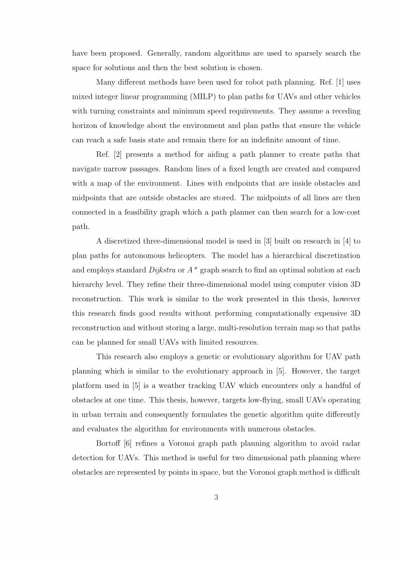
with trailers and the Alpha 1.0 Puzzle [16]. The RRT algorithm quickly searches the
space of possible solutions by extending a tree in random directions as described in
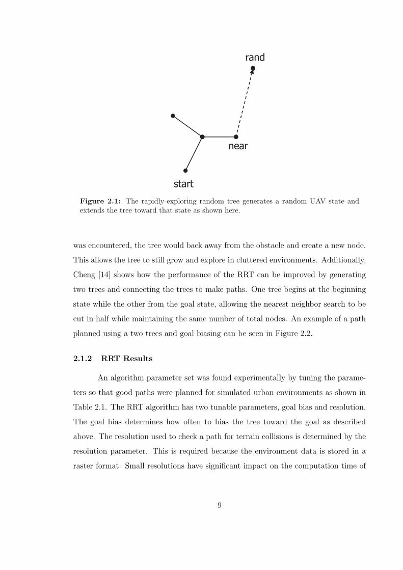
Algorithm 1 and shown in Figure 2.1.
2.1.1 RRT Algorithm Description
When RRTs are used for UAV path planning, the tree nodes are potential UAV
waypoints and the branches are paths to the waypoints. A tree is initially composed
of the UAV’s position as a single node. A random UAV state is generated and the
tree is extended toward the random point creating a new branch and node as outlined
in Algorithm 1. When a path is found or a maximum number of iterations is reached,
the RRT terminates.
Algorithm 1 Rapidly-Exploring Random Trees
1: Initialize a tree containing one node – the starting location of the UAV2: while A path has not been found do3: rand = A random UAV state4: near = The state in the tree that is closest to rand5: if the tree can be connected from near to rand without collision then6: extend the tree from near to rand7: end if8: end while
RRTs can be biased toward the goal point by occasionally substituting the
goal for the randomly chosen state. However, the goal should be used infrequently to
enable the tree to grow randomly and explore the solution space. The nearest neighbor
search is O(n2) and is the most computationally intense part of the algorithm. The
basic RRT algorithm is improved by extending the tree in the direction of the random
point instead of only connecting to collision free points. In the event that an obstacle
8
start
near
rand
Figure 2.1: The rapidly-exploring random tree generates a random UAV state andextends the tree toward that state as shown here.
was encountered, the tree would back away from the obstacle and create a new node.
This allows the tree to still grow and explore in cluttered environments. Additionally,
Cheng [14] shows how the performance of the RRT can be improved by generating
two trees and connecting the trees to make paths. One tree begins at the beginning
state while the other from the goal state, allowing the nearest neighbor search to be
cut in half while maintaining the same number of total nodes. An example of a path
planned using a two trees and goal biasing can be seen in Figure 2.2.
2.1.2 RRT Results
An algorithm parameter set was found experimentally by tuning the parame-
ters so that good paths were planned for simulated urban environments as shown in
Table 2.1. The RRT algorithm has two tunable parameters, goal bias and resolution.
The goal bias determines how often to bias the tree toward the goal as described
above. The resolution used to check a path for terrain collisions is determined by the
resolution parameter. This is required because the environment data is stored in a
raster format. Small resolutions have significant impact on the computation time of
9
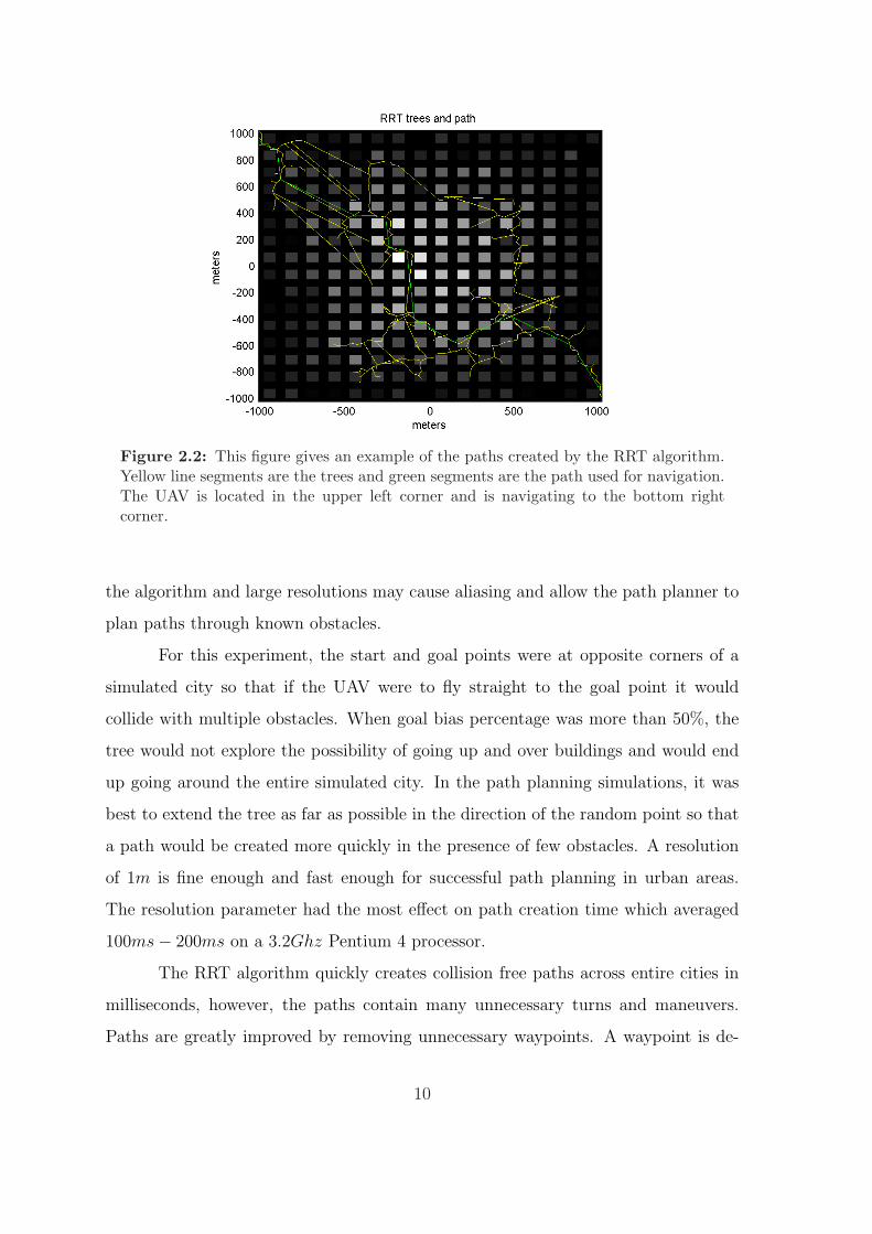
Figure 2.2: This figure gives an example of the paths created by the RRT algorithm.Yellow line segments are the trees and green segments are the path used for navigation.The UAV is located in the upper left corner and is navigating to the bottom rightcorner.
the algorithm and large resolutions may cause aliasing and allow the path planner to
plan paths through known obstacles.
For this experiment, the start and goal points were at opposite corners of a
simulated city so that if the UAV were to fly straight to the goal point it would
collide with multiple obstacles. When goal bias percentage was more than 50%, the
tree would not explore the possibility of going up and over buildings and would end
up going around the entire simulated city. In the path planning simulations, it was
best to extend the tree as far as possible in the direction of the random point so that
a path would be created more quickly in the presence of few obstacles. A resolution
of 1m is fine enough and fast enough for successful path planning in urban areas.
The resolution parameter had the most effect on path creation time which averaged
100ms− 200ms on a 3.2Ghz Pentium 4 processor.
The RRT algorithm quickly creates collision free paths across entire cities in
milliseconds, however, the paths contain many unnecessary turns and maneuvers.
Paths are greatly improved by removing unnecessary waypoints. A waypoint is de-
10
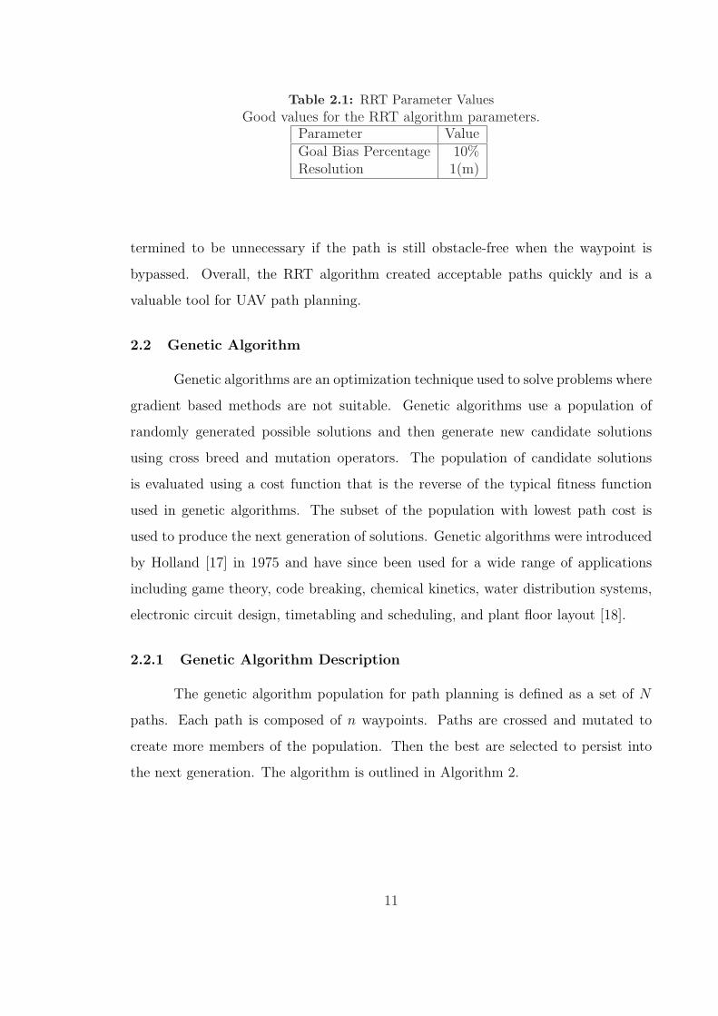
Table 2.1: RRT Parameter ValuesGood values for the RRT algorithm parameters.
Parameter ValueGoal Bias Percentage 10%Resolution 1(m)
termined to be unnecessary if the path is still obstacle-free when the waypoint is
bypassed. Overall, the RRT algorithm created acceptable paths quickly and is a
valuable tool for UAV path planning.
2.2 Genetic Algorithm
Genetic algorithms are an optimization technique used to solve problems where
gradient based methods are not suitable. Genetic algorithms use a population of
randomly generated possible solutions and then generate new candidate solutions
using cross breed and mutation operators. The population of candidate solutions
is evaluated using a cost function that is the reverse of the typical fitness function
used in genetic algorithms. The subset of the population with lowest path cost is
used to produce the next generation of solutions. Genetic algorithms were introduced
by Holland [17] in 1975 and have since been used for a wide range of applications
including game theory, code breaking, chemical kinetics, water distribution systems,
electronic circuit design, timetabling and scheduling, and plant floor layout [18].
2.2.1 Genetic Algorithm Description
The genetic algorithm population for path planning is defined as a set of N
paths. Each path is composed of n waypoints. Paths are crossed and mutated to
create more members of the population. Then the best are selected to persist into
the next generation. The algorithm is outlined in Algorithm 2.
11
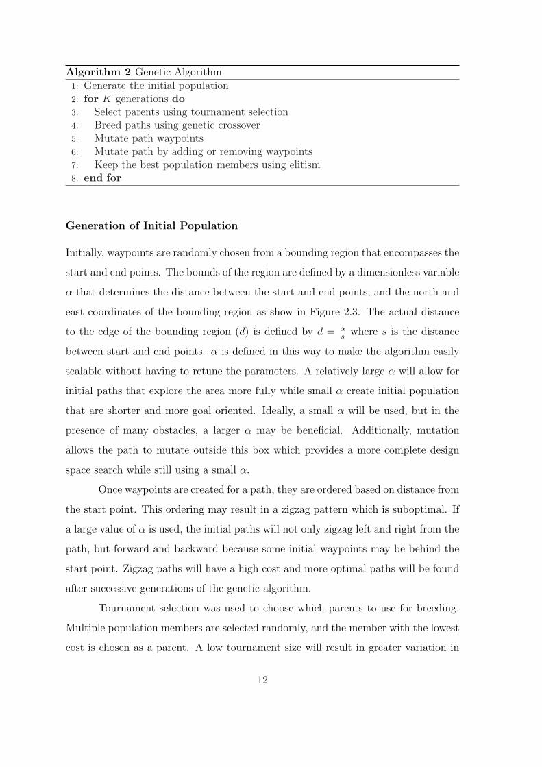
Algorithm 2 Genetic Algorithm
1: Generate the initial population2: for K generations do3: Select parents using tournament selection4: Breed paths using genetic crossover5: Mutate path waypoints6: Mutate path by adding or removing waypoints7: Keep the best population members using elitism8: end for
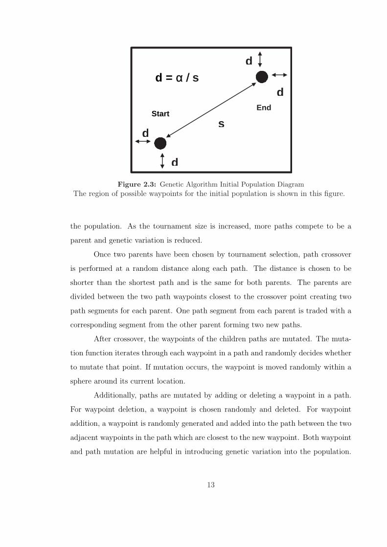
Generation of Initial Population
Initially, waypoints are randomly chosen from a bounding region that encompasses the
start and end points. The bounds of the region are defined by a dimensionless variable
α that determines the distance between the start and end points, and the north and
east coordinates of the bounding region as show in Figure 2.3. The actual distance
to the edge of the bounding region (d) is defined by d = αs
where s is the distance
between start and end points. α is defined in this way to make the algorithm easily
scalable without having to retune the parameters. A relatively large α will allow for
initial paths that explore the area more fully while small α create initial population
that are shorter and more goal oriented. Ideally, a small α will be used, but in the
presence of many obstacles, a larger α may be beneficial. Additionally, mutation
allows the path to mutate outside this box which provides a more complete design
space search while still using a small α.
Once waypoints are created for a path, they are ordered based on distance from
the start point. This ordering may result in a zigzag pattern which is suboptimal. If
a large value of α is used, the initial paths will not only zigzag left and right from the
path, but forward and backward because some initial waypoints may be behind the
start point. Zigzag paths will have a high cost and more optimal paths will be found
after successive generations of the genetic algorithm.
Tournament selection was used to choose which parents to use for breeding.
Multiple population members are selected randomly, and the member with the lowest
cost is chosen as a parent. A low tournament size will result in greater variation in
12
d
d
d
d
s
d = α / α / α / α / s
Start End
Figure 2.3: Genetic Algorithm Initial Population DiagramThe region of possible waypoints for the initial population is shown in this figure.
the population. As the tournament size is increased, more paths compete to be a
parent and genetic variation is reduced.
Once two parents have been chosen by tournament selection, path crossover
is performed at a random distance along each path. The distance is chosen to be
shorter than the shortest path and is the same for both parents. The parents are
divided between the two path waypoints closest to the crossover point creating two
path segments for each parent. One path segment from each parent is traded with a
corresponding segment from the other parent forming two new paths.
After crossover, the waypoints of the children paths are mutated. The muta-
tion function iterates through each waypoint in a path and randomly decides whether
to mutate that point. If mutation occurs, the waypoint is moved randomly within a
sphere around its current location.
Additionally, paths are mutated by adding or deleting a waypoint in a path.
For waypoint deletion, a waypoint is chosen randomly and deleted. For waypoint
addition, a waypoint is randomly generated and added into the path between the two
adjacent waypoints in the path which are closest to the new waypoint. Both waypoint
and path mutation are helpful in introducing genetic variation into the population.
13
If a path from the initial population intersects the terrain, mutation can modify or
create points that bypass the obstacle.
The cost of the path is determined by
c = (s + kcVc − kdVd)(1 + p · i) (2.1)
using the length of the path (s), the vertical climb (Vc), the descent (Vd), the number
of path segments that intersect the terrain (i), the climb factor (kc), the descent
factor (kd) and the penalty for a terrain intersection (p). This function is minimized
to provide the path of least distance and fewest terrain collisions. For the experiments
shown in this document we used kc = 1, kd = 0.1, p = 2. This function works well
for path planning because it rewards paths of shorter length while assigning a high
penalty to terrain collisions. This may not be a good cost function in the event
that there is a thin obstacle that is difficult to fly over or around, but flying straight
through is a short path. If the cost to fly around or over the obstacle is (p + 1) times
as much as flying straight through, the path with the collision will have a lower cost.
Increasing p decreases the possibility of accepting a terrain collision. Using a terrain
collision penalty that multiplies the path length provides a scalable algorithm.
After crossover and mutation, children are added to the population, although
they are not candidates for tournament selection until the next generation. The 2N
paths in the population are then ordered by cost and the N paths with the lowest
cost are chosen to propagate to the next generation. This genetic algorithm has the
following parameters.
• Number of generations
• Population size
• Tournament size
• Waypoint mutation probability
• Maximum waypoint mutation
14
• Waypoint addition probability
• Waypoint deletion probability
• α
• Initial number of waypoints
The number of generations determines the maximum number of generations to allow
the population to evolve. Tournament size is the size of the group in which to find
the most fit parents. Maximum waypoint mutation is the largest distance to mutate
the waypoint. α is used to generate initial population as in Figure 2.3. The initial
number of waypoints is the number of waypoints that each initial path contains.
2.2.2 Genetic Algorithm Results
A parameter set that would result in a feasible path most of the time was found
experimentally and the results are shown in Table 2.2. For these experiments, the
UAV began in the center of the simulated city, surrounded by tall buildings and was
commanded to get to a goal point outside the city. The goal point was located such
that if the UAV navigated directly to the goal it would encounter multiple obstacles.
After finding a default set of parameters, high and low values (shown in Table 2.2)
for each of the parameters were tested to see which parameters had the most effect
on the algorithm. During the analysis the same random seed was used and only the
parameter of interest was varied from the default.
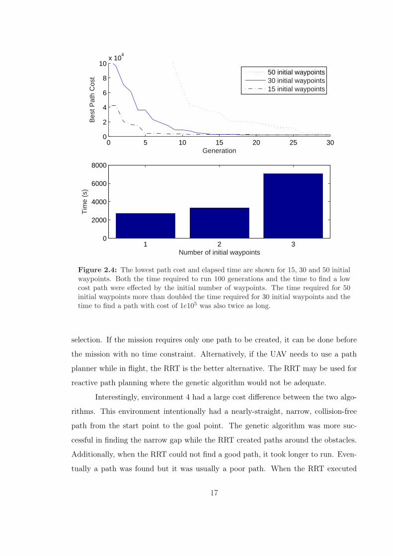
The effectiveness of the genetic algorithm path planner is highly sensitive
to the initial number of waypoints. Figure 2.4 shows that more initial waypoints
substantially increased the time required to compute each generation and the time
to find a path with a low cost. Tournament size and population size also have a
significant effect on the success and run time of the algorithm. The final parameter
value in Table 2.2 indicates values that were chosen after evaluating the effect of each
parameter.
Figure 2.5 shows a sequence of screen shots of the paths from the generations of
the genetic algorithm. The images are taken after the 1st, 15th, and 30th generations.
15
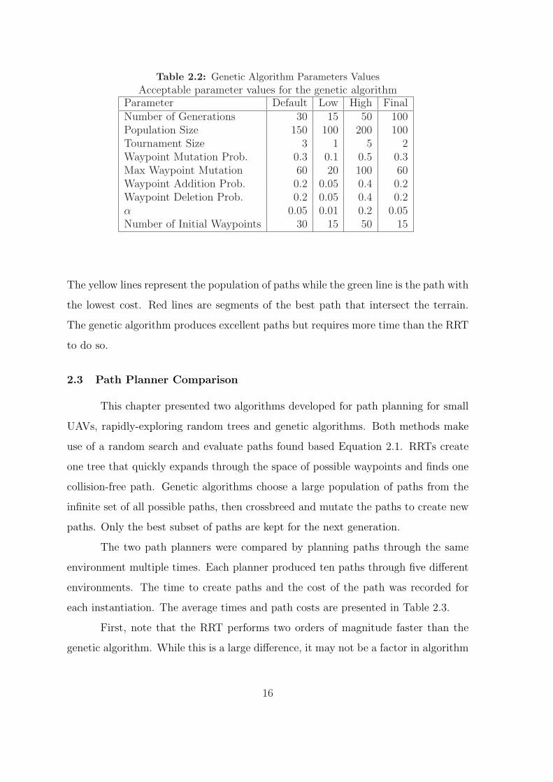
Table 2.2: Genetic Algorithm Parameters ValuesAcceptable parameter values for the genetic algorithm
Parameter Default Low High FinalNumber of Generations 30 15 50 100Population Size 150 100 200 100Tournament Size 3 1 5 2Waypoint Mutation Prob. 0.3 0.1 0.5 0.3Max Waypoint Mutation 60 20 100 60Waypoint Addition Prob. 0.2 0.05 0.4 0.2Waypoint Deletion Prob. 0.2 0.05 0.4 0.2α 0.05 0.01 0.2 0.05Number of Initial Waypoints 30 15 50 15
The yellow lines represent the population of paths while the green line is the path with
the lowest cost. Red lines are segments of the best path that intersect the terrain.
The genetic algorithm produces excellent paths but requires more time than the RRT
to do so.
2.3 Path Planner Comparison
This chapter presented two algorithms developed for path planning for small
UAVs, rapidly-exploring random trees and genetic algorithms. Both methods make
use of a random search and evaluate paths found based Equation 2.1. RRTs create
one tree that quickly expands through the space of possible waypoints and finds one
collision-free path. Genetic algorithms choose a large population of paths from the
infinite set of all possible paths, then crossbreed and mutate the paths to create new
paths. Only the best subset of paths are kept for the next generation.
The two path planners were compared by planning paths through the same
environment multiple times. Each planner produced ten paths through five different
environments. The time to create paths and the cost of the path was recorded for
each instantiation. The average times and path costs are presented in Table 2.3.
First, note that the RRT performs two orders of magnitude faster than the
genetic algorithm. While this is a large difference, it may not be a factor in algorithm
16
0 5 10 15 20 25 300
2
4
6
8
10x 10
4
Generation
Bes
t Pat
h C
ost
50 initial waypoints30 initial waypoints15 initial waypoints
1 2 30
2000
4000
6000
8000
Tim
e (s
)
Number of initial waypoints
Figure 2.4: The lowest path cost and elapsed time are shown for 15, 30 and 50 initialwaypoints. Both the time required to run 100 generations and the time to find a lowcost path were effected by the initial number of waypoints. The time required for 50initial waypoints more than doubled the time required for 30 initial waypoints and thetime to find a path with cost of 1e105 was also twice as long.
selection. If the mission requires only one path to be created, it can be done before
the mission with no time constraint. Alternatively, if the UAV needs to use a path
planner while in flight, the RRT is the better alternative. The RRT may be used for
reactive path planning where the genetic algorithm would not be adequate.
Interestingly, environment 4 had a large cost difference between the two algo-
rithms. This environment intentionally had a nearly-straight, narrow, collision-free
path from the start point to the goal point. The genetic algorithm was more suc-
cessful in finding the narrow gap while the RRT created paths around the obstacles.
Additionally, when the RRT could not find a good path, it took longer to run. Even-
tually a path was found but it was usually a poor path. When the RRT executed
17
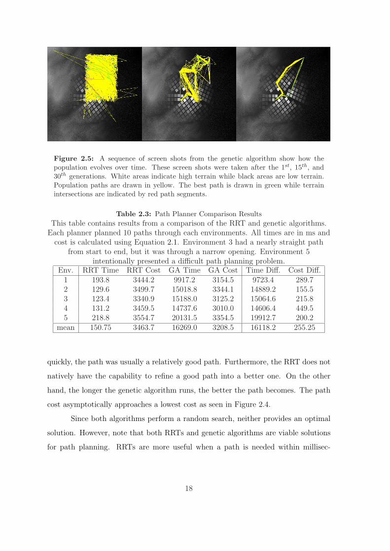
Figure 2.5: A sequence of screen shots from the genetic algorithm show how thepopulation evolves over time. These screen shots were taken after the 1st, 15th, and30th generations. White areas indicate high terrain while black areas are low terrain.Population paths are drawn in yellow. The best path is drawn in green while terrainintersections are indicated by red path segments.
Table 2.3: Path Planner Comparison ResultsThis table contains results from a comparison of the RRT and genetic algorithms.
Each planner planned 10 paths through each environments. All times are in ms andcost is calculated using Equation 2.1. Environment 3 had a nearly straight path
from start to end, but it was through a narrow opening. Environment 5intentionally presented a difficult path planning problem.
Env. RRT Time RRT Cost GA Time GA Cost Time Diff. Cost Diff.1 193.8 3444.2 9917.2 3154.5 9723.4 289.72 129.6 3499.7 15018.8 3344.1 14889.2 155.53 123.4 3340.9 15188.0 3125.2 15064.6 215.84 131.2 3459.5 14737.6 3010.0 14606.4 449.55 218.8 3554.7 20131.5 3354.5 19912.7 200.2
mean 150.75 3463.7 16269.0 3208.5 16118.2 255.25
quickly, the path was usually a relatively good path. Furthermore, the RRT does not
natively have the capability to refine a good path into a better one. On the other
hand, the longer the genetic algorithm runs, the better the path becomes. The path
cost asymptotically approaches a lowest cost as seen in Figure 2.4.
Since both algorithms perform a random search, neither provides an optimal
solution. However, note that both RRTs and genetic algorithms are viable solutions
for path planning. RRTs are more useful when a path is needed within millisec-
18
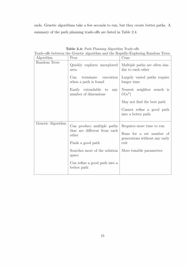
onds. Genetic algorithms take a few seconds to run, but they create better paths. A
summary of the path planning trade-offs are listed in Table 2.4.
Table 2.4: Path Planning Algorithm Trade-offsTrade-offs between the Genetic algorithm and the Rapidly-Exploring Random Trees.Algorithm Pros ConsRandom Trees
Quickly explores unexploredarea
Can terminate executionwhen a path is found
Easily extendable to anynumber of dimensions
Multiple paths are often sim-ilar to each other
Largely varied paths requirelonger time
Nearest neighbor search isO(n2)
May not find the best path
Cannot refine a good pathinto a better path
Genetic AlgorithmCan produce multiple pathsthat are different from eachother
Finds a good path
Searches more of the solutionspace
Can refine a good path into abetter path
Requires more time to run
Runs for a set number ofgenerations without any earlyexit
More tunable parameters
19

20
Chapter 3
Feature Tracking
Not all information about a UAV’s mission can be known before the mission.
Publicly available terrain elevation data is low resolution which implies that large
objects such as buildings are not represented. Large metropolitan areas appear as
small bumps in this elevation data. Additionally, even if high resolution data is
available, it may not contain recent changes to the environment like new construction
or other landscape developments. Moreover, if a GPS sensor has a 10m bias, the
actual location may be different from the estimated location of the UAV. Finally,
information about a given area may not be available at all. Any of these situations
require the UAV to sense and avoid obstacles in the environment.
To successfully navigate, a low-flying UAV must obtain three dimensional in-
formation about its surroundings. Possible options for acquiring this data are laser
range finders, optical flow sensors, and landscape reconstruction from video and fea-
ture tracking. Current laser range finder hardware works well, but is too heavy to
be flown on a micro UAV. Optical flow sensors are small and low power, but only
provide one optical flow measurement at each sample. This limits the capability to
determine where a UAV can and cannot fly. These sensors are also incapable of
providing useful information when pointed straight forward because optical flow is
small and would flow outward from the center providing one net measurement of zero
optical flow. While inferior to a laser range finder, three-dimensional reconstruction
provides a good estimate of the UAV’s environment. However, it cannot be performed
fast enough to navigate a small UAV in urban terrain. Feature tracking provides even
less information than three-dimensional reconstruction about the UAV’s environment,
but substantially more than optical flow sensors. More attractively, feature tracking
21
can be performed in real time and can be used to guide a small UAV past obstacles
in its path. Feature tracking was originally introduced by Moravec [19].
3.1 Feature Detection
Instead of computing an optical flow vector for each pixel or for each region of
pixels, feature tracking is a method of computing optical flow for visually interesting
pixels. Each pixel is assigned a value based on how easily it can be tracked and then
a small window around the pixel is correlated in subsequent frames to relocate the
same image feature at its new location. The velocity of the image feature in pixels
and the movement of the camera in the world allows the three dimensional location
of the image feature to be calculated and mapped.
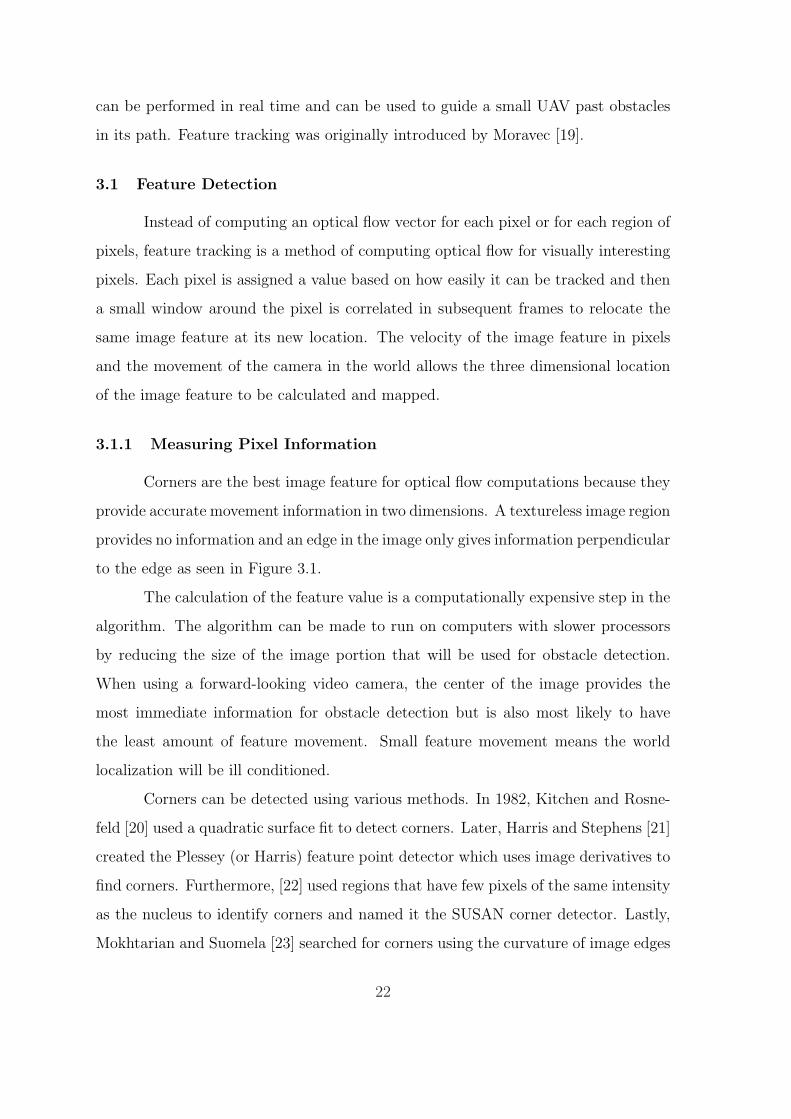
3.1.1 Measuring Pixel Information
Corners are the best image feature for optical flow computations because they
provide accurate movement information in two dimensions. A textureless image region
provides no information and an edge in the image only gives information perpendicular
to the edge as seen in Figure 3.1.
The calculation of the feature value is a computationally expensive step in the
algorithm. The algorithm can be made to run on computers with slower processors
by reducing the size of the image portion that will be used for obstacle detection.
When using a forward-looking video camera, the center of the image provides the
most immediate information for obstacle detection but is also most likely to have
the least amount of feature movement. Small feature movement means the world
localization will be ill conditioned.
Corners can be detected using various methods. In 1982, Kitchen and Rosne-
feld [20] used a quadratic surface fit to detect corners. Later, Harris and Stephens [21]
created the Plessey (or Harris) feature point detector which uses image derivatives to
find corners. Furthermore, [22] used regions that have few pixels of the same intensity
as the nucleus to identify corners and named it the SUSAN corner detector. Lastly,
Mokhtarian and Suomela [23] searched for corners using the curvature of image edges
22
Figure 3.1: Corners are the best image feature for optical flow computations becausethey provide accurate movement information in two dimensions while edges provideinformation along one dimension.
in what is now called Curvature Scale Space (CSS) corner detection. Analysis of
these and other corner detectors has been done previously and is beyond the scope
of this research. For algorithm comparison, see [23]. The Harris Corner Detector
is included in the OpenCV [24] library and was used for this this research. A more
detailed explaination of this algorithm follows.
3.1.2 Harris Corner Detector
The feature strength is calculated using the Harris Edge and Corner Detector
described in ref. [21]. This corner detector uses the moment matrix
Mij =
I2
x Ixy
Iyx I2y
(3.1)
of the vertical and horizontal image gradients at each pixel to determine if the pixel
is an edge, corner or untextured region. In Equation 3.1, Ix and Iy are the image
gradients in the horizontal and vertical directions respectively of the grayscale image
I1. I is the average over a square window of the image. The moment matrix is then
23
used in
Rij = det|Mij| − 0.04(I2x + I2
y )2 (3.2)
to calculate feature strength R. Small values for R are untextured areas, while large
negative numbers are edges and large positive numbers are corners.
3.2 Feature Selection
The pixels with the largest feature strength are selected for tracking. However,
based on the movement of the camera, there will potentially be one pixel that will
not provide any optical flow information even if it has a high feature value because
the feature will not move in the image coordinates. This pixel is called the epipole
and is the pixel that is inline with the translational motion of the camera. When a
UAV is flying straight with a forward facing camera the epipole is in the center of
the image. A linear weighting could be used to bias feature selection away from the
epipole when necessary.
Additionally, one good image corner produces multiple neighboring pixels with
high feature strength. The pixel with the highest feature strength is selected and the
feature strength of neighboring pixels is set to zero so that the same image feature
isn’t selected multiple times.
Only the best features from each frame will be located in subsequent frames.
The n pixels with the highest feature value are the correct features to track, but an
efficient algorithm for selecting those features from a raster format is not obvious. A
brute force search for the best n features in an image containing N pixels is O(N ·n).
A more cache-efficient method is to insert the pixels into a list sorted by feature value.
If the list is limited to length n, O(N log(n)) can be achieved. However, since one
image corner produces multiple pixels with high feature value, the first few features
on the list will correspond to the same image corner. An image proximity check is
necessary when inserting image features into the list to ensure neighboring pixels will
not be used. With this addition, the order of the number of computations is back to
O(N · n). This method has the same computational order as the more simple, brute
24
force method, but is more cache-efficient because the entire image will only need to
be loaded into cache once.
3.3 Image Correlation
Image correlation is performed when a second video frame (I2) is available for
processing. The feature window saved from the first video frame (I1) is correlated
using the pseudo-normalized correlation function
c =2∑
I1I2∑I21 +
∑I22
(3.3)
as derived by Moravec in ref. [25]. The pixel with the highest correlation value is
then used to perform a biquadratic fit using
q = ax2 + by2 + cxy + dx + ey + f (3.4)
to fit a 3x3 neighborhood of pixels where q is a correlation score, x is the column
index, and y is the row index. The coefficients a-f are found by using a least squares
algorithm. The subpixel maximum of the fitted surface is then found by partial
differentiation, which leads to the following solution for x and y:
x = (−2bd + ce)/(4ab− c2) (3.5)
and
y = (−2ae + cd)/(4ab− c2). (3.6)
The biquadratic fit allows image correlation to achieve subpixel accuracy.
The implementation first verifies that the pixel-resolution maximum occurs at
an interior location, then computes the subpixel maximum and verifies that the sub-
pixel maximum is within one pixel of the pixel-resolution maximum. The covariance
of the fit is used as a metric of how good the fit is. The number of incorrect corre-
25
lations that are accepted is reduced significantly by using a relatively high threshold
for the fit value.
3.4 Feature Tracking for Obstacle Avoidance
To allow vehicles to avoid obstacles, image features need to be localized in
world coordinates. To localize image features in world coordinates, the pixel loca-
tion of the features in images corresponding to telemetry must be known. Video
is captured at 30Hz while telemetry is transmitted between 10Hz to 1Hz so there
will be multiple frames between each telemetry packet. Therefore, features found in
one image must ultimately be located multiple images later. If intermediate images
are ignored, a large search window must be used to re-find the features in the second
telemetry frame. If features are tracked through every frame, a smaller search window
may be used. However, when features are found with subpixel resolution, the location
is rounded to the discrete pixel grid. The accuracy of the image correlations at the
second telemetry frame is highly affected by rounding at each frame. To alleviate this
error, the location found by tracking through every frame can be used as an estimate
for a final image correlation. The final image correlation is performed on the image
where the feature was originally found instead of the previous frame. This method
allows for subpixel resolution, small window sizes, and accurate image correlations.
3.4.1 Window size and frequency of tracking
The time to compute the image correlations is proportional to the area of the
search window or the square of the window size. It is desirable to minimize the size of
the search window. However, if a small search window is used, features may be lost
due to large feature movements in the image frame. Figure 3.2 shows an overhead
view of the movement of a vehicle that would cause feature movement in the image
frame. In Figure 3.2, p1 and p2 are the image pixel locations of the obstacle feature.
Note how the pixel location moves in image coordinates from frame 1 to frame 2.
26
θ2θ1
s1
s2
p1p2
d
Obstacle
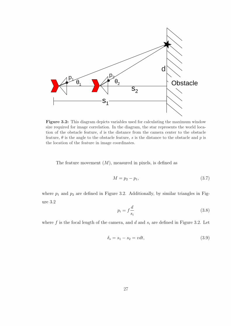
Figure 3.2: This diagram depicts variables used for calculating the maximum windowsize required for image correlation. In the diagram, the star represents the world loca-tion of the obstacle feature, d is the distance from the camera center to the obstaclefeature, θ is the angle to the obstacle feature, s is the distance to the obstacle and p isthe location of the feature in image coordinates.
The feature movement (M), measured in pixels, is defined as
M = p2 − p1, (3.7)
where p1 and p2 are defined in Figure 3.2. Additionally, by similar triangles in Fig-
ure 3.2
pi = fd
si
(3.8)
where f is the focal length of the camera, and d and si are defined in Figure 3.2. Let
δs = s1 − s2 = vdt, (3.9)
27
where v is the velocity of the UAV and dt is the time difference between telemetry
updates. Feature movement is derived from Equation 3.7 as follows,
M = fd
s2
− fd
s1
, (3.10)
= fds
s1
tan θ2, (3.11)
= f(s1 − s2)d
s1s2
, (3.12)
= fvdt
s2 + vdttan θ2. (3.13)
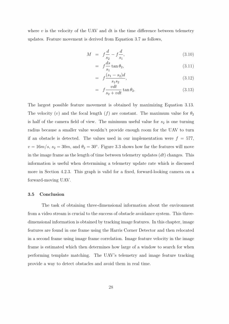
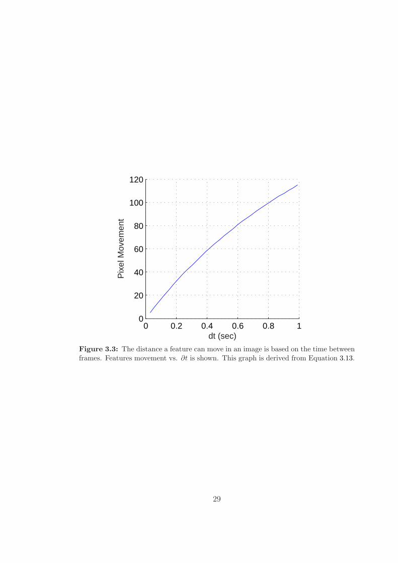
The largest possible feature movement is obtained by maximizing Equation 3.13.
The velocity (v) and the focal length (f) are constant. The maximum value for θ2
is half of the camera field of view. The minimum useful value for s2 is one turning
radius because a smaller value wouldn’t provide enough room for the UAV to turn
if an obstacle is detected. The values used in our implementation were f = 577,
v = 16m/s, s2 = 30m, and θ2 = 30◦. Figure 3.3 shows how far the features will move
in the image frame as the length of time between telemetry updates (dt) changes. This
information is useful when determining a telemetry update rate which is discussed
more in Section 4.2.3. This graph is valid for a fixed, forward-looking camera on a
forward-moving UAV.
3.5 Conclusion
The task of obtaining three-dimensional information about the environment
from a video stream is crucial to the success of obstacle avoidance system. This three-
dimensional information is obtained by tracking image features. In this chapter, image
features are found in one frame using the Harris Corner Detector and then relocated
in a second frame using image frame correlation. Image feature velocity in the image
frame is estimated which then determines how large of a window to search for when
performing template matching. The UAV’s telemetry and image feature tracking
provide a way to detect obstacles and avoid them in real time.
28
0 0.2 0.4 0.6 0.8 10
20
40
60
80
100
120
dt (sec)
Pix
el M
ovem
ent
Figure 3.3: The distance a feature can move in an image is based on the time betweenframes. Features movement vs. ∂t is shown. This graph is derived from Equation 3.13.
29

30
Chapter 4
Obstacle Detection
The goal of obstacle detection is to use feature movement in the image and
camera motion or UAV telemetry to localize a three dimensional no-fly zone to prevent
the UAV from colliding with a stationary object. Feature movement is provided by
the image processing described in Chapter 3 and UAV telemetry is available from on-
board sensors. The accuracy of UAV telemetry for small UAVs is not always reliable
because highly accurate sensors and estimators are expensive, large and heavy. A
new state estimation algorithm incorporating a more complete dynamic model is
currently being developed by Eldredge [26] which will greatly improve the accuracy
of the telemetry. This chapter presents two methods for localizing obstacles: three-
dimensional ray intersection and depth from motion.
4.1 Preliminaries
Before describing the obstacle detection algorithms, some mathematical pre-
liminaries are included for reference and for completeness. First, transformation ma-
trices are useful when converting between image coordinates and world coordinates.
Next, a convenient representation for rays and planes is also included. Finally, a
cylindrical representation for obstacles is presented and equations for ray-cylinder in-
tersections are given. Most of these preliminaries are found at Mathworld.com from
Wolfram Research [27].
Multiple coordinate transformations are required to convert from pixel coordi-
nates to camera, body, vehicle, or world coordinates. These transformations depend
on the attitude of the UAV and the location of the camera on the UAV and the
camera calibration matrix. This work uses the matrices outlined by Redding [28] to
31
calculate transformations. When transforming the two dimensional pixel data into
three dimensional coordinates only a ray originating at the camera center extending
in the direction of the pixel can be obtained.
In three dimensions, a ray is best represented using the parametric form of a
line. This parametric form is
x = xo + xdk (4.1)
or
x
y
z
=
xo
yo
zo
+
xd
yd
zd
k (4.2)
where x, xo and xd are vectors with three values. The variable x represents a point
on the ray, xo is the starting point for the ray and xd is the direction of the ray.
A plane in space can be represented multiple ways. The normal form is given
by
nT(x− xo) = 0 (4.3)
where n is a vector normal to the plane and xo is a point on the plane. Equivalently,
a plane can be represented by the general form,
Ax + By + Cz + D = 0 (4.4)
where A, B, C and D are scalars. Any point (x, y, z) that satisfies Equation 4.4 is on
the plane. Converting between the forms is accomplished by setting
A = nx,
B = ny,
C = nz, (4.5)
D = −n · xo.
32
A cylinder is a convenient representation for UAV obstacles because path inter-
sections with cylinders are computationally easily. Furthermore, cylinders are simple
to navigate around because the UAV can use a circular orbit flight trajectory based
on a cross section of the cylinder, or use an altitude climb based on the height of the
cylinder. Spheres do not have the capability to represent tall and thin or short and
wide obstacles. Bounding boxes can represent a cluster of feature points well, but are
not as easy to use for path intersection and UAV navigation.
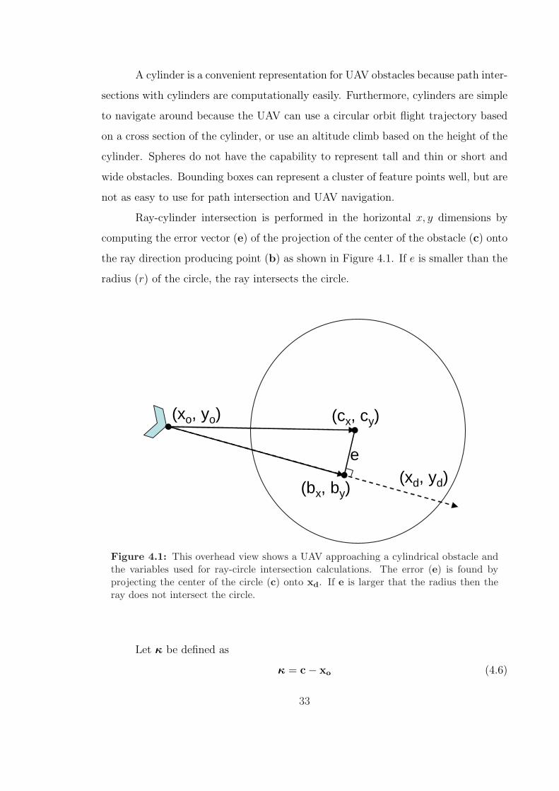
Ray-cylinder intersection is performed in the horizontal x, y dimensions by
computing the error vector (e) of the projection of the center of the obstacle (c) onto
the ray direction producing point (b) as shown in Figure 4.1. If e is smaller than the
radius (r) of the circle, the ray intersects the circle.
e
(cx, cy)
(xd, yd)
(xo, yo)
(bx, by)
Figure 4.1: This overhead view shows a UAV approaching a cylindrical obstacle andthe variables used for ray-circle intersection calculations. The error (e) is found byprojecting the center of the circle (c) onto xd. If e is larger that the radius then theray does not intersect the circle.
Let κ be defined as
κ = c− xo (4.6)
33
where c is the center of the circle and xo is the origin of the ray. Also, let β be defined
as
β = b− xo. (4.7)
Then β can be found by projection κ onto xd:
β =κ · xd
‖xd‖2xd. (4.8)
The error of the projection is given by
e = κ− β (4.9)
and
= κ− κ · xd
‖xd‖2xd. (4.10)
If ‖e‖ is smaller that r then the ray intersects the circle with positive or negative
values of k. If the dot product
κ · β (4.11)
is positive then the ray intersects the circle for positive values of k, i.e., in front of
the UAV.
4.2 Obstacle Detection Using Three Dimensional Ray Intersection
When the same image feature is found in multiple frames, the pixel coordi-
nate from each frame can be transformed into a ray originating at the UAV location
pointing in the direction of the feature pixel. The intersection of two rays determines
the world location of that feature as shown in Figure 4.2. The location of the UAV
can be provided by GPS and the ray direction is calculated using the attitude of the
airplane. The direction of the ray is highly sensitive to the accuracy of UAV roll,
pitch and yaw estimates.
34
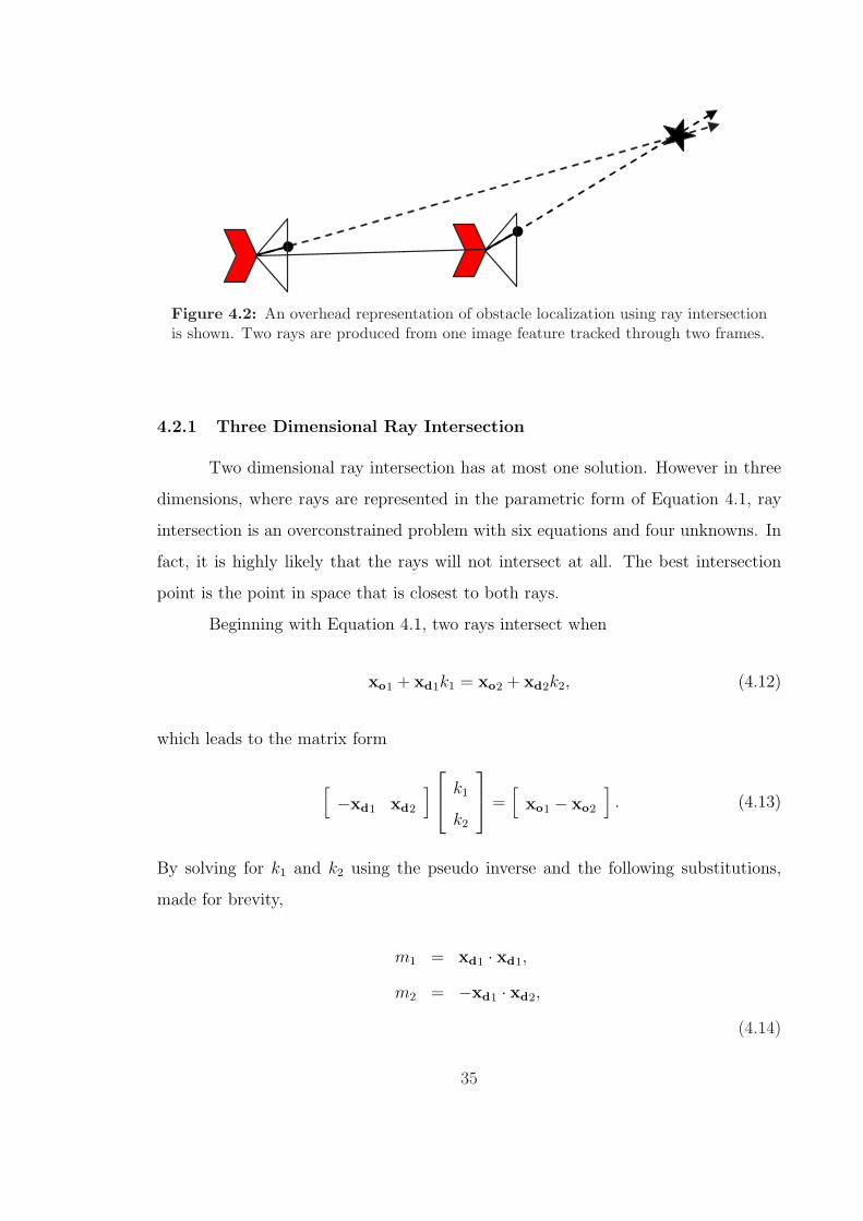
Figure 4.2: An overhead representation of obstacle localization using ray intersectionis shown. Two rays are produced from one image feature tracked through two frames.
4.2.1 Three Dimensional Ray Intersection
Two dimensional ray intersection has at most one solution. However in three
dimensions, where rays are represented in the parametric form of Equation 4.1, ray
intersection is an overconstrained problem with six equations and four unknowns. In
fact, it is highly likely that the rays will not intersect at all. The best intersection
point is the point in space that is closest to both rays.
Beginning with Equation 4.1, two rays intersect when
xo1 + xd1k1 = xo2 + xd2k2, (4.12)
which leads to the matrix form
[−xd1 xd2
] k1
k2
=
[xo1 − xo2
]. (4.13)
By solving for k1 and k2 using the pseudo inverse and the following substitutions,
made for brevity,
m1 = xd1 · xd1,
m2 = −xd1 · xd2,
(4.14)
35
m3 = −xd1 · xd2 = m2,
m4 = xd2 · xd2,
t = xo1 − xo2,
s1 = xd1 · t,s2 = xd2 · t.
Equation 4.13 becomes
k1
k2
=
1
m1m4 −m2m3
m4 −m2
−m3 m1
s1
s2
. (4.15)
The values of k1 and k2 are used in Equation 4.1 to get one point from each ray. The
two points are averaged to find the point in space that is closest to the two original
rays.
4.2.2 Feature Clustering
Ray intersection uses three-dimensional rays created from multiple matching
feature pairs and telemetry to create a point cloud in three dimensional space. The
number of points is equal to the number of features that were successfully tracked
between frames. The three dimensional points need to be grouped into obstacles so
that the UAV can safely navigate around potential obstacles. Clustering algorithms
such as K-means [29] or Fuzzy Clustering [30] require the knowledge of the number of
groups which is unavailable for our application. Therefore, a hierarchial clustering [31]
algorithm is used.
There are two types of hierarchial clustering: agglomerative and divisive. Di-
visive clustering divides the group until groups are smaller than a threshold size.
Agglomerative clustering begins with each point in a separate group and combines
groups until they are all farther than a fixed distance from all other groups. Agglom-
erative clustering is well suited for UAV obstacle avoidance applications because it
ensures that all groups are a threshold distance from other groups. This allows the
36
UAV to ensure that there is enough room to maneuver between obstacles that are
detected. The threshold distance depends on the dynamics and capabilities of the
UAV. As a general rule, the threshold should be at least one turning radius.
4.2.3 The Ill Conditioned Nature of This Problem
Ray intersection calculations as presented here are highly sensitive to error
in telemetry because the ray intersection matrix is ill conditioned because the rays
point generally in the same direction. Increased velocity and increased time between
telemetry packets helps the ray intersection calculation, but makes image feature
tracking more difficult. The best solution is to use a longer time between packets
and to track features in every frame. This will enable the image correlation window
to remain small while having a better conditioned matrix pseudo inverse. However,
when the UAV is close to an obstacle, the obstacle will move greater distances in the
image and a shorter time between packets would be desirable. An analysis of the
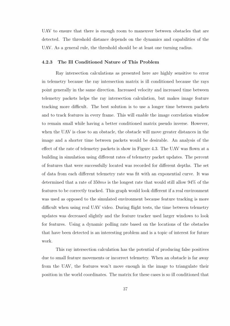
effect of the rate of telemetry packets is show in Figure 4.3. The UAV was flown at a
building in simulation using different rates of telemetry packet updates. The percent
of features that were successfully located was recorded for different depths. The set
of data from each different telemetry rate was fit with an exponential curve. It was
determined that a rate of 350ms is the longest rate that would still allow 94% of the
features to be correctly tracked. This graph would look different if a real environment
was used as opposed to the simulated environment because feature tracking is more
difficult when using real UAV video. During flight tests, the time between telemetry
updates was decreased slightly and the feature tracker used larger windows to look
for features. Using a dynamic polling rate based on the locations of the obstacles
that have been detected is an interesting problem and is a topic of interest for future
work.
This ray intersection calculation has the potential of producing false positives
due to small feature movements or incorrect telemetry. When an obstacle is far away
from the UAV, the features won’t move enough in the image to triangulate their
position in the world coordinates. The matrix for these cases is so ill conditioned that
37
20 40 60 80 100 120 1400.8
0.82
0.84
0.86
0.88
0.9
0.92
0.94
0.96
0.98
1
distance to obstacle
perc
ent o
f fea
ture
s co
rrec
tly tr
acke
d
200 ms300 ms400 ms600 ms800 ms
Figure 4.3: The UAV was flown at a simulated building using different telemetrypacket update rates and the percentage of features that were tracked correctly wasrecorded. This data was fit with exponential curves as seen in this figure. An updaterate of 350ms is the longest rate that gives adequate feature tracking.
the triangulated point could be anywhere along the pixel ray. A minimum feature
pixel movement constraint wouldn’t be sufficient because when the UAV turns, there
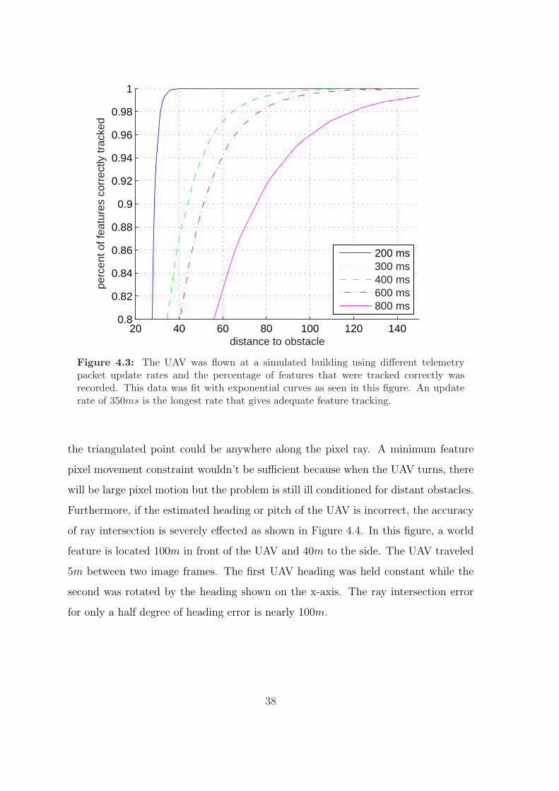
will be large pixel motion but the problem is still ill conditioned for distant obstacles.
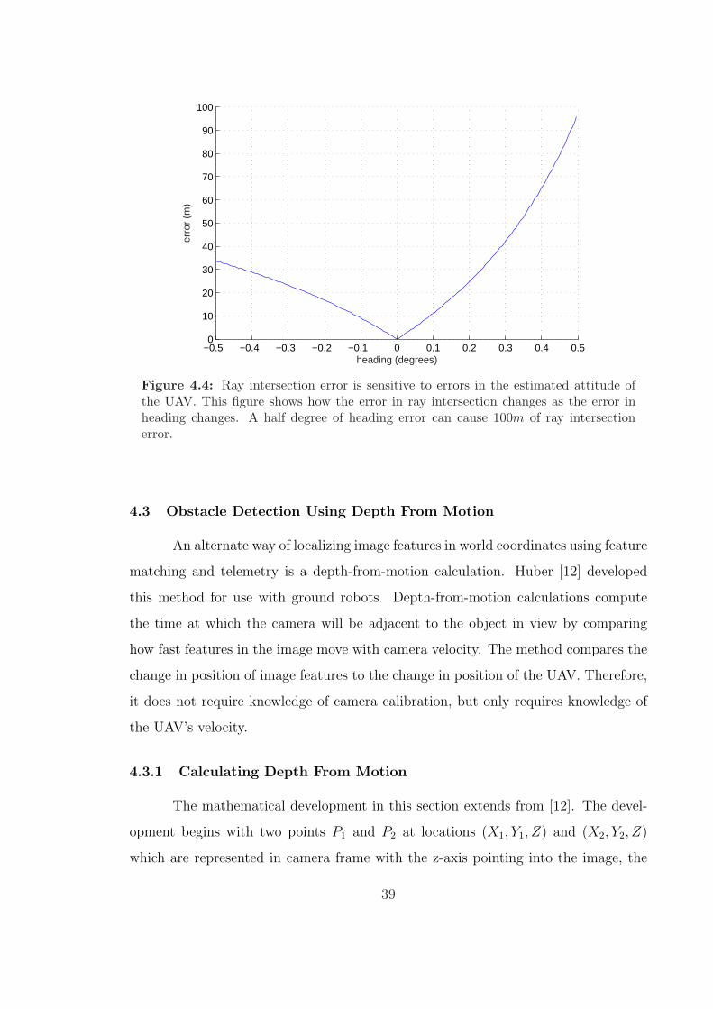
Furthermore, if the estimated heading or pitch of the UAV is incorrect, the accuracy
of ray intersection is severely effected as shown in Figure 4.4. In this figure, a world
feature is located 100m in front of the UAV and 40m to the side. The UAV traveled
5m between two image frames. The first UAV heading was held constant while the
second was rotated by the heading shown on the x-axis. The ray intersection error
for only a half degree of heading error is nearly 100m.
38
−0.5 −0.4 −0.3 −0.2 −0.1 0 0.1 0.2 0.3 0.4 0.50
10
20
30
40
50
60
70
80
90
100
heading (degrees)
erro
r (m
)
Figure 4.4: Ray intersection error is sensitive to errors in the estimated attitude ofthe UAV. This figure shows how the error in ray intersection changes as the error inheading changes. A half degree of heading error can cause 100m of ray intersectionerror.
4.3 Obstacle Detection Using Depth From Motion
An alternate way of localizing image features in world coordinates using feature
matching and telemetry is a depth-from-motion calculation. Huber [12] developed
this method for use with ground robots. Depth-from-motion calculations compute
the time at which the camera will be adjacent to the object in view by comparing
how fast features in the image move with camera velocity. The method compares the
change in position of image features to the change in position of the UAV. Therefore,
it does not require knowledge of camera calibration, but only requires knowledge of
the UAV’s velocity.
4.3.1 Calculating Depth From Motion
The mathematical development in this section extends from [12]. The devel-
opment begins with two points P1 and P2 at locations (X1, Y1, Z) and (X2, Y2, Z)
which are represented in camera frame with the z-axis pointing into the image, the
39
x-axis pointing left and the y-axis pointing down. Note that it is assumed that the
points are at the same depth. The corresponding image points are
p1 = (xc + fX1
Z, yc + f
Y1
Z) and (4.16)
p2 = (xc + fX2
Z, yc + f
Y2
Z). (4.17)
Let
B = ‖P1 − P2‖ and (4.18)
b = ‖p1 − p2‖ , then (4.19)
b =
∥∥∥∥(
fX1
Z− f
X2
Z, f
Y1
Z− f
Y2
Z
)∥∥∥∥ (4.20)
b = fB
Z, (4.21)
db
dZ= −f
B
Z2and (4.22)
db
dt=
db
dZ
dZ
dt= −f
B
Z2
dZ
dt= − b
Z
dZ
dt. (4.23)
In Equation 4.23, the movement of the features in the image frame (dbdt
), the movement
of the UAV (dZdt
) and the distance between the image features (b) are all known, leaving
only the depth of the object (Z) unknown. Solving Equation 4.23 for Z yields
Z = − b
db/dZ. (4.24)
Formulating the equation in this way assumes that all the image feature movement is
correlated with the movement of the UAV. However, some image features movement
will be caused by rotation of the UAV. This method assumes that the camera is
moving in translational motion only.
Only two features are required to calculate the depth of the object. If many
features are present, the average depth can be calculated by computing depths for all
pairs and averaging all depths. If features do not move in the image frame, they will
not be useful for depth calculations. This happens when world objects are far away
40
from the UAV or are near the epipole of the camera movement. All features that do
not move more than a threshold distance must be removed, because if the feature
does not move, it could be at any depth.
4.3.2 Handling Obstacles of Multiple Depths
One immediate detriment of this method is that it assumes all features are at
the same depth. If objects are not at the same world depth, an erroneous depth esti-
mate will be calculated. One method of dividing the features into different obstacles
is to compute the depths for each pair of features and then use the RANSAC [32]
algorithm to choose a set of inlier points that agree on the depth. RANSAC can be
used again on the outliers to see if there is another set of features that computes the
same depth. However, features on objects of different depths compute an incorrect
depth which will then be erroneously categorized. The incorrect depth is a function of
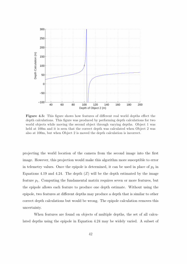
where the features are in relation to each other in the image frame. Figure 4.5 shows
the sensitivity of the depth computation to features of different depths. This figure
was produced by performing depth calculations for two world objects while moving
the second object through varying depths. Object 1 was held at 100m and it is seen
that the correct depth was calculated when Object 2 was also at 100m, but when
Object 2 is moved from 30m to 200m, the depth calculation is greatly effected. In
fact, when the two objects are located such that they project to the same image coor-
dinate, there are infinite solutions. Figure 4.5 was deliberately crafted to show high
sensitivity, but this type of error is certainly possible. While the depth calculation is
not always so highly effected, it is always a factor.
Obstacles of multiple depths can be more effectively handled using the epipole
of the camera motion. An epipole is created when the camera is moved from one
location to another. The epipole is the center of the translational movement of the
features in the image plane. It is also the location of the first camera in the second
image or the location of the second camera in the first image. Mathematically, the
epipole is the null space of the fundamental matrix which can be calculated using
matching feature points as in [33]. Alternatively, the epipole can be determined by
41
40 60 80 100 120 140 160 180 200−100
−50
0
50
100
150
200
250
300
Depth of Object 2 (m)
Dep
th C
alcu
latio
n (m
)
Figure 4.5: This figure shows how features of different real world depths effect thedepth calculations. This figure was produced by performing depth calculations for twoworld objects while moving the second object through varying depths. Object 1 washeld at 100m and it is seen that the correct depth was calculated when Object 2 wasalso at 100m, but when Object 2 is moved the depth calculation is incorrect.
projecting the world location of the camera from the second image into the first
image. However, this projection would make this algorithm more susceptible to error
in telemetry values. Once the epipole is determined, it can be used in place of p2 in
Equations 4.19 and 4.24. The depth (Z) will be the depth estimated by the image
feature p1. Computing the fundamental matrix requires seven or more features, but
the epipole allows each feature to produce one depth estimate. Without using the
epipole, two features at different depths may produce a depth that is similar to other
correct depth calculations but would be wrong. The epipole calculation removes this
uncertainty.
When features are found on objects of multiple depths, the set of all calcu-
lated depths using the epipole in Equation 4.24 may be widely varied. A subset of
42
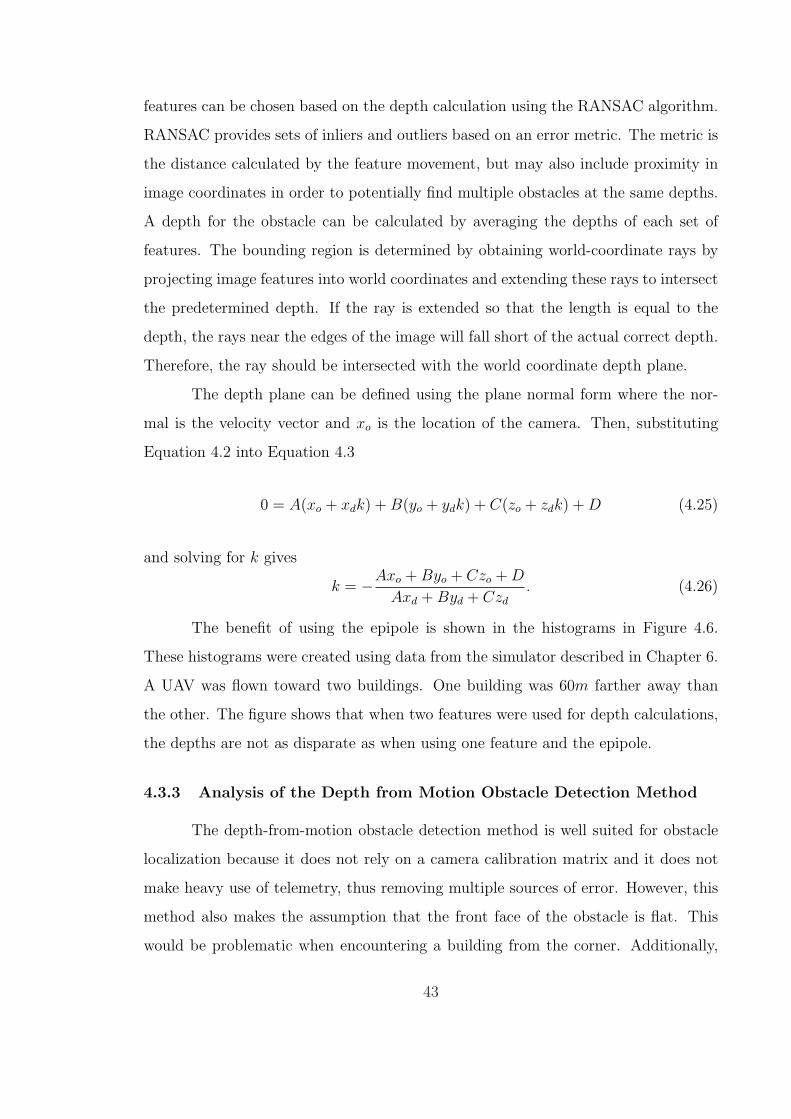
features can be chosen based on the depth calculation using the RANSAC algorithm.
RANSAC provides sets of inliers and outliers based on an error metric. The metric is
the distance calculated by the feature movement, but may also include proximity in
image coordinates in order to potentially find multiple obstacles at the same depths.
A depth for the obstacle can be calculated by averaging the depths of each set of
features. The bounding region is determined by obtaining world-coordinate rays by
projecting image features into world coordinates and extending these rays to intersect
the predetermined depth. If the ray is extended so that the length is equal to the
depth, the rays near the edges of the image will fall short of the actual correct depth.
Therefore, the ray should be intersected with the world coordinate depth plane.
The depth plane can be defined using the plane normal form where the nor-
mal is the velocity vector and xo is the location of the camera. Then, substituting
Equation 4.2 into Equation 4.3
0 = A(xo + xdk) + B(yo + ydk) + C(zo + zdk) + D (4.25)
and solving for k gives
k = −Axo + Byo + Czo + D
Axd + Byd + Czd
. (4.26)
The benefit of using the epipole is shown in the histograms in Figure 4.6.
These histograms were created using data from the simulator described in Chapter 6.
A UAV was flown toward two buildings. One building was 60m farther away than
the other. The figure shows that when two features were used for depth calculations,
the depths are not as disparate as when using one feature and the epipole.
4.3.3 Analysis of the Depth from Motion Obstacle Detection Method
The depth-from-motion obstacle detection method is well suited for obstacle
localization because it does not rely on a camera calibration matrix and it does not
make heavy use of telemetry, thus removing multiple sources of error. However, this
method also makes the assumption that the front face of the obstacle is flat. This
would be problematic when encountering a building from the corner. Additionally,
43
it assumes that the UAV is not turning or rotating which is rarely the case for small
UAVs.
4.4 Conclusion
Two methods for detecting obstacles using UAV telemetry and image feature
tracking were presented. Three-dimensional ray intersection accounts for image frame
rotations, but is ill conditioned and therefore sensitive to noise. The depth-from-
motion algorithm provides a good depth estimate, but assumes camera translation
only and is sensitive to camera rotation. Both algorithms take little time to run
when compared with image feature tracking, but depth-from-motion is simpler to
implement. For results on how well each algorithm detects obstacles, see Chapter 7.
44
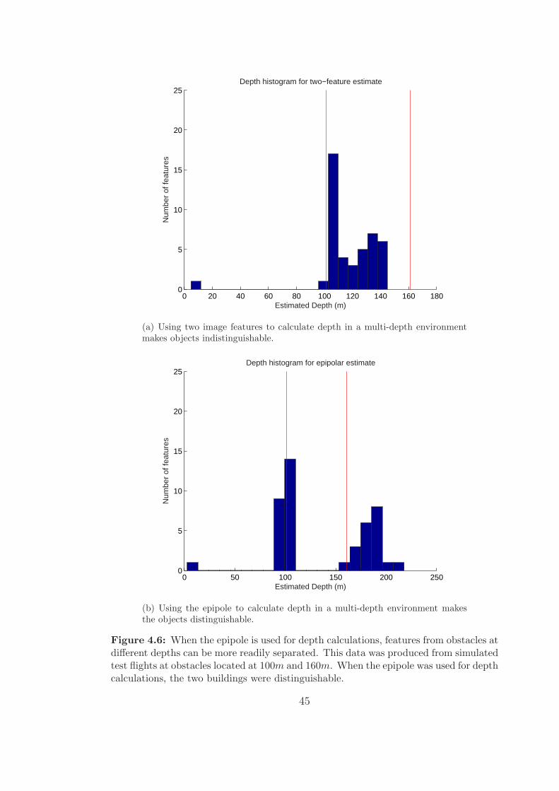
0 20 40 60 80 100 120 140 160 1800
5
10
15
20
25Depth histogram for two−feature estimate
Estimated Depth (m)
Num
ber
of fe
atur
es
(a) Using two image features to calculate depth in a multi-depth environmentmakes objects indistinguishable.
0 50 100 150 200 2500
5
10
15
20
25Depth histogram for epipolar estimate
Estimated Depth (m)
Num
ber
of fe
atur
es
(b) Using the epipole to calculate depth in a multi-depth environment makesthe objects distinguishable.
Figure 4.6: When the epipole is used for depth calculations, features from obstacles atdifferent depths can be more readily separated. This data was produced from simulatedtest flights at obstacles located at 100m and 160m. When the epipole was used for depthcalculations, the two buildings were distinguishable.
45

46
Chapter 5
Obstacle Avoidance
5.1 Sliding Mode Orbit Controller
Once obstacles have been grouped and mapped from pixel to world coordi-
nates, each of the obstacles are checked for intersection with the waypoint path. The
position and radius of the cylinder representing the object that intersects the way-
point path at the point closest to the UAV is then passed as an input to the reactive
avoidance controller. When the reactive avoidance controller receives an input it
overrides the waypoint navigation controller with course commands from the sliding
mode controller described by
χc = χ +1
α
(Vg
δsin (χ− γ) + c
k
(1 + k (δ − r))2Vg cos (χ− γ) +κ
αsat
(χ
ε
))(5.1)
where χ is defined as χd − χ, k is a tunable parameter that controls the convergence
rate of the vector field, κ is a tunable parameter that controls the reactiveness of the
controller to tracking errors in course, and ε is a tunable parameter that controls the
width of the sliding mode around the nominal radius r. Other terms in the control
equation are defined as shown in Figure 5.1.
Nelson et al. [34] showed that this control law would cause asymptotic conver-
gence of the UAV course to the vector field described by
χd = γ + c(π
2− tan−1 (k (δ − r))
). (5.2)
The parameter c in Equation 5.1 represents the direction of the orbit with c = 1
corresponding to a clockwise orbit and c = −1 corresponding to a counterclockwise
47
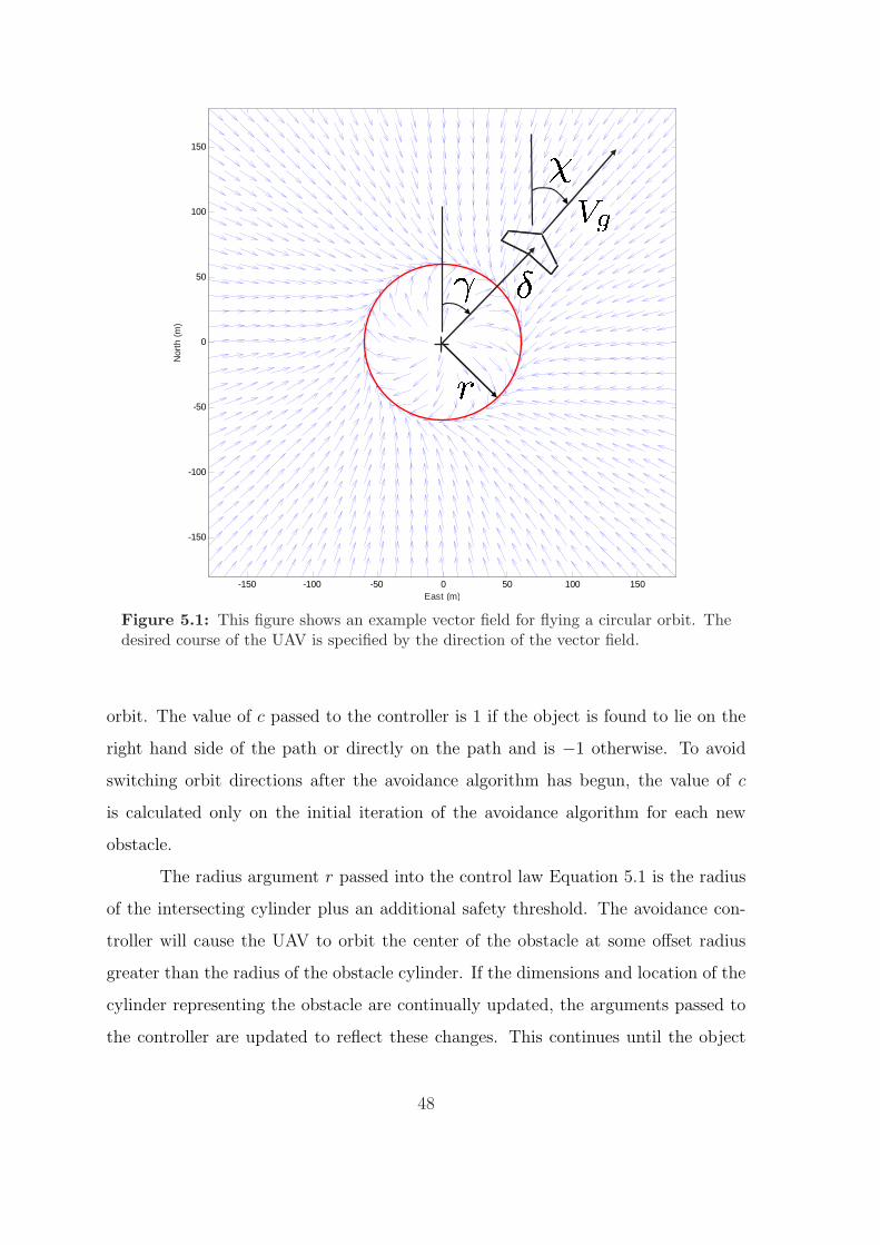
-150 -100 -50 0 50 100 150
-150
-100
-50
0
50
100
150
East (m)
Nor
th (
m)
-150 -100 -50 0 50 100 150
-150
-100
-50
0
50
100
150
East (m)
Nor
th (
m)
Figure 5.1: This figure shows an example vector field for flying a circular orbit. Thedesired course of the UAV is specified by the direction of the vector field.
orbit. The value of c passed to the controller is 1 if the object is found to lie on the
right hand side of the path or directly on the path and is −1 otherwise. To avoid
switching orbit directions after the avoidance algorithm has begun, the value of c
is calculated only on the initial iteration of the avoidance algorithm for each new
obstacle.
The radius argument r passed into the control law Equation 5.1 is the radius
of the intersecting cylinder plus an additional safety threshold. The avoidance con-
troller will cause the UAV to orbit the center of the obstacle at some offset radius
greater than the radius of the obstacle cylinder. If the dimensions and location of the
cylinder representing the obstacle are continually updated, the arguments passed to
the controller are updated to reflect these changes. This continues until the object
48
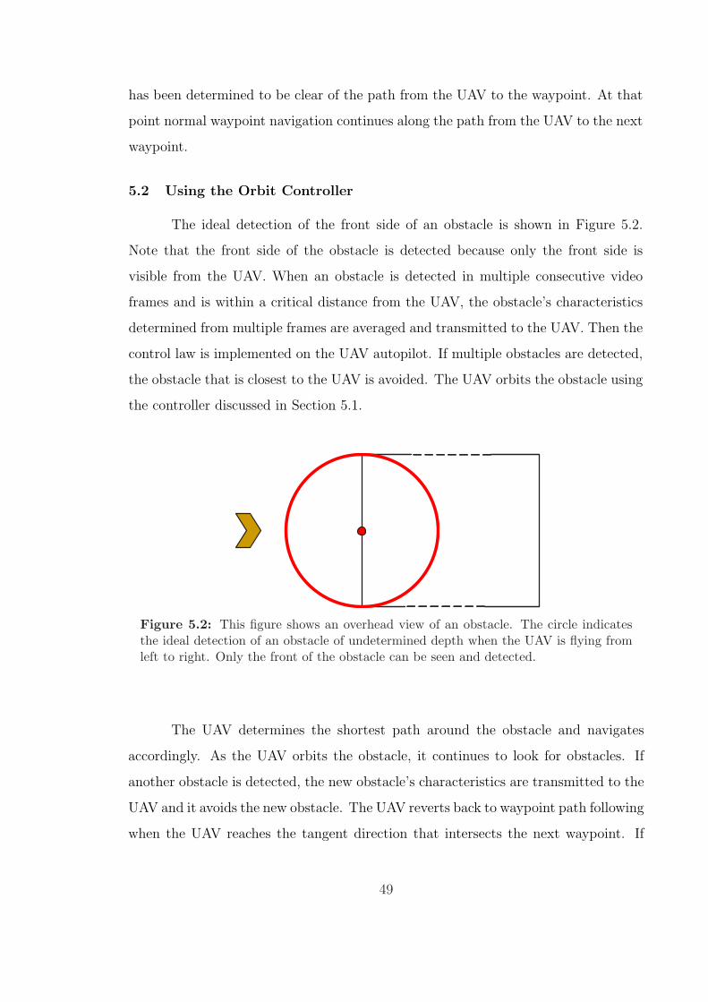
has been determined to be clear of the path from the UAV to the waypoint. At that
point normal waypoint navigation continues along the path from the UAV to the next
waypoint.
5.2 Using the Orbit Controller
The ideal detection of the front side of an obstacle is shown in Figure 5.2.
Note that the front side of the obstacle is detected because only the front side is
visible from the UAV. When an obstacle is detected in multiple consecutive video
frames and is within a critical distance from the UAV, the obstacle’s characteristics
determined from multiple frames are averaged and transmitted to the UAV. Then the
control law is implemented on the UAV autopilot. If multiple obstacles are detected,
the obstacle that is closest to the UAV is avoided. The UAV orbits the obstacle using
the controller discussed in Section 5.1.
Figure 5.2: This figure shows an overhead view of an obstacle. The circle indicatesthe ideal detection of an obstacle of undetermined depth when the UAV is flying fromleft to right. Only the front of the obstacle can be seen and detected.
The UAV determines the shortest path around the obstacle and navigates
accordingly. As the UAV orbits the obstacle, it continues to look for obstacles. If
another obstacle is detected, the new obstacle’s characteristics are transmitted to the
UAV and it avoids the new obstacle. The UAV reverts back to waypoint path following
when the UAV reaches the tangent direction that intersects the next waypoint. If
49
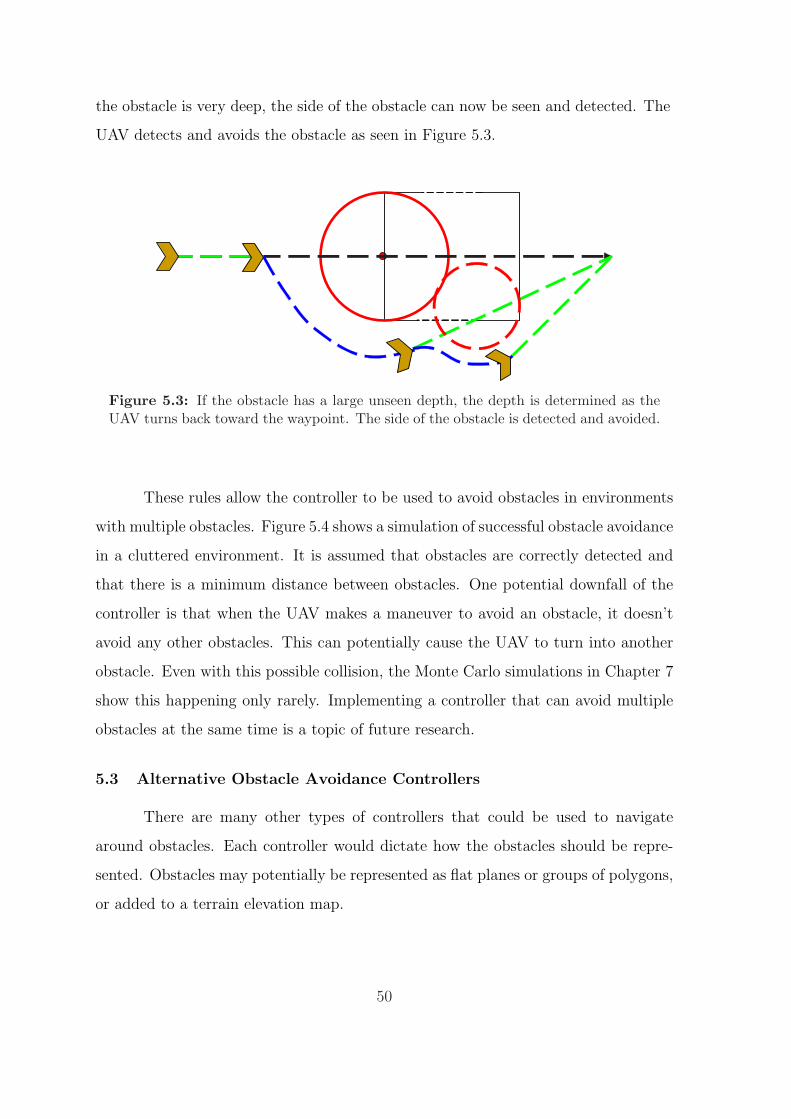
the obstacle is very deep, the side of the obstacle can now be seen and detected. The
UAV detects and avoids the obstacle as seen in Figure 5.3.
Figure 5.3: If the obstacle has a large unseen depth, the depth is determined as theUAV turns back toward the waypoint. The side of the obstacle is detected and avoided.
These rules allow the controller to be used to avoid obstacles in environments
with multiple obstacles. Figure 5.4 shows a simulation of successful obstacle avoidance
in a cluttered environment. It is assumed that obstacles are correctly detected and
that there is a minimum distance between obstacles. One potential downfall of the
controller is that when the UAV makes a maneuver to avoid an obstacle, it doesn’t
avoid any other obstacles. This can potentially cause the UAV to turn into another
obstacle. Even with this possible collision, the Monte Carlo simulations in Chapter 7
show this happening only rarely. Implementing a controller that can avoid multiple
obstacles at the same time is a topic of future research.
5.3 Alternative Obstacle Avoidance Controllers
There are many other types of controllers that could be used to navigate
around obstacles. Each controller would dictate how the obstacles should be repre-
sented. Obstacles may potentially be represented as flat planes or groups of polygons,
or added to a terrain elevation map.
50
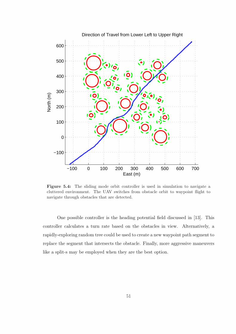
−100 0 100 200 300 400 500 600 700
−100
0
100
200
300
400
500
600
Direction of Travel from Lower Left to Upper Right
East (m)
Nor
th (
m)
Figure 5.4: The sliding mode orbit controller is used in simulation to navigate acluttered environment. The UAV switches from obstacle orbit to waypoint flight tonavigate through obstacles that are detected.
One possible controller is the heading potential field discussed in [13]. This
controller calculates a turn rate based on the obstacles in view. Alternatively, a
rapidly-exploring random tree could be used to create a new waypoint path segment to
replace the segment that intersects the obstacle. Finally, more aggressive maneuvers
like a split-s may be employed when they are the best option.
51
5.4 Conclusion
A sliding mode controller used for obstacle avoidance is discussed. The con-
troller is used when an obstacle is detected. Otherwise the UAV navigates a waypoint
path. This controller only navigates around one obstacle at a time and may have dif-
ficulty in environments with multiple closely-spaced obstacles. This controller does
not consider flying above obstacles but a rule could be implemented to allow such
navigation.
52
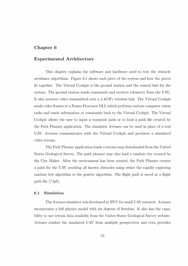
Chapter 6
Experimental Architecture
This chapter explains the software and hardware used to test the obstacle
avoidance algorithms. Figure 6.1 shows each piece of the system and how the pieces
fit together. The Virtual Cockpit is the ground station and the central hub for the
system. The ground station sends commands and receives telemetry from the UAV.
It also receives video transmitted over a 2.4GHz wireless link. The Virtual Cockpit
sends video frames to a Frame Processor DLL which performs various computer vision
tasks and sends information or commands back to the Virtual Cockpit. The Virtual
Cockpit allows the user to input a waypoint path or to load a path file created by
the Path Planner application. The simulator Aviones can be used in place of a real
UAV. Aviones communicates with the Virtual Cockpit and produces a simulated
video stream.
The Path Planner application loads a terrain map downloaded from the United
States Geological Survey. The path planner may also load a random city created by
the City Maker. After the environment has been created, the Path Planner creates
a path for the UAV avoiding all known obstacles using either the rapidly exploring
random tree algorithm or the genetic algorithm. The flight path is saved as a flight
path file (*.fpf).
6.1 Simulation
The Aviones simulator was developed at BYU for small UAV research. Aviones
incorporates a full physics model with six degrees of freedom. It also has the capa-
bility to use terrain data available from the Unites States Geological Survey website.
Aviones renders the simulated UAV from multiple perspectives and even provides
53
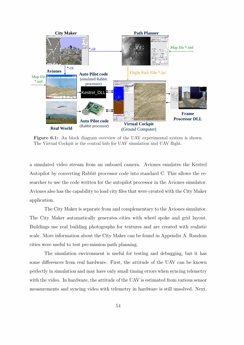
Aviones
Virtual Cockpit(Ground Computer)Real World
Path Planner
*.cit
Map file *.tmf
*.cit
Flight Path File *.fpf
Map file *.tmf
City Maker
Kestrel_DLL
Auto Pilot code(Rabbit processor)
Auto Pilot code(emulated Rabbit
processor)
Frame Processor DLL
Figure 6.1: An block diagram overview of the UAV experimental system is shown.The Virtual Cockpit is the central hub for UAV simulation and UAV flight.
a simulated video stream from an onboard camera. Aviones emulates the Kestrel
Autopilot by converting Rabbit processor code into standard C. This allows the re-
searcher to use the code written for the autopilot processor in the Aviones simulator.
Aviones also has the capability to load city files that were created with the City Maker
application.
The City Maker is separate from and complementary to the Aviones simulator.
The City Maker automatically generates cities with wheel spoke and grid layout.
Buildings use real building photographs for textures and are created with realistic
scale. More information about the City Maker can be found in Appendix A. Random
cities were useful to test pre-mission path planning.
The simulation environment is useful for testing and debugging, but it has
some differences from real hardware. First, the attitude of the UAV can be known
perfectly in simulation and may have only small timing errors when syncing telemetry
with the video. In hardware, the attitude of the UAV is estimated from various sensor
measurements and syncing video with telemetry in hardware is still unsolved. Next,
54
external forces such as wind can be eliminated in simulation while there will always
be some unknown disturbance in hardware.
6.2 Hardware
The airframe used in this research is a 1.1m wingspan foam flying wing man-
ufactured by Unicorn Wings [35] shown in Figure 6.2, which was selected for its
durability and ease of component installation. The UAV is controlled by an em-
bedded Kestrel Autopilot (Figure 6.3) from Procerus [36] which has a Rabbit 3400
29MHz processor, rate gyros, accelerometers, absolute and differential pressure sen-
sors. The autopilot measures 3.8cm x 5.1cm x 1.9cm and weighs 18g. The autopilot
communicates with the ground station using a 1000mW , 900MHz radio modem. The
autopilot also makes use of an external Furuno [37] GPS module for navigation. This
research also uses a Black Widow [38] camera with a 2.4GHz analog transmission
to a directional ground antenna. The video is then sent into an Imperx [39] digi-
tal frame grabber and displayed in the Virtual Cockpit ground station software. A
Hewlett Packard [40] Pavillion zd8000 notebook computer with a Pentium 4, 3.2GHz
processor and 1GB of RAM was used for the ground station and performed the image
processing and obstacle detection routines.
Figure 6.2: A foam airframe manufactured by Unicorn Wings was modified and usedfor this research.
55
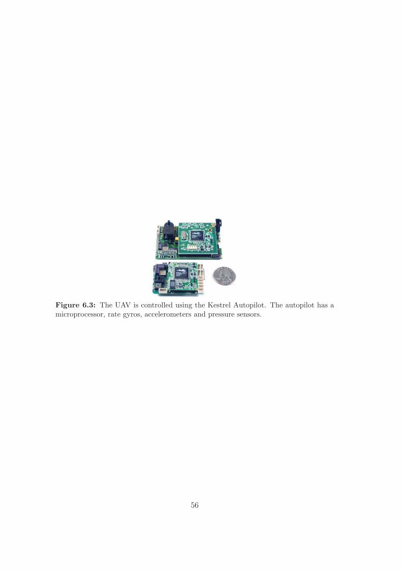
Figure 6.3: The UAV is controlled using the Kestrel Autopilot. The autopilot has amicroprocessor, rate gyros, accelerometers and pressure sensors.
56
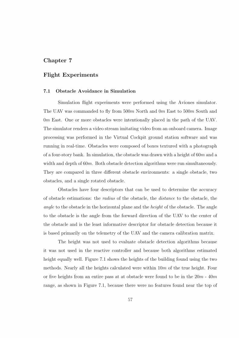
Chapter 7
Flight Experiments
7.1 Obstacle Avoidance in Simulation
Simulation flight experiments were performed using the Aviones simulator.
The UAV was commanded to fly from 500m North and 0m East to 500m South and
0m East. One or more obstacles were intentionally placed in the path of the UAV.
The simulator renders a video stream imitating video from an onboard camera. Image
processing was performed in the Virtual Cockpit ground station software and was
running in real-time. Obstacles were composed of boxes textured with a photograph
of a four-story bank. In simulation, the obstacle was drawn with a height of 60m and a
width and depth of 60m. Both obstacle detection algorithms were run simultaneously.
They are compared in three different obstacle environments: a single obstacle, two
obstacles, and a single rotated obstacle.
Obstacles have four descriptors that can be used to determine the accuracy
of obstacle estimations: the radius of the obstacle, the distance to the obstacle, the
angle to the obstacle in the horizontal plane and the height of the obstacle. The angle
to the obstacle is the angle from the forward direction of the UAV to the center of
the obstacle and is the least informative descriptor for obstacle detection because it
is based primarily on the telemetry of the UAV and the camera calibration matrix.
The height was not used to evaluate obstacle detection algorithms because
it was not used in the reactive controller and because both algorithms estimated
height equally well. Figure 7.1 shows the heights of the building found using the two
methods. Nearly all the heights calculated were within 10m of the true height. Four
or five heights from an entire pass at at obstacle were found to be in the 20m - 40m
range, as shown in Figure 7.1, because there were no features found near the top of
57
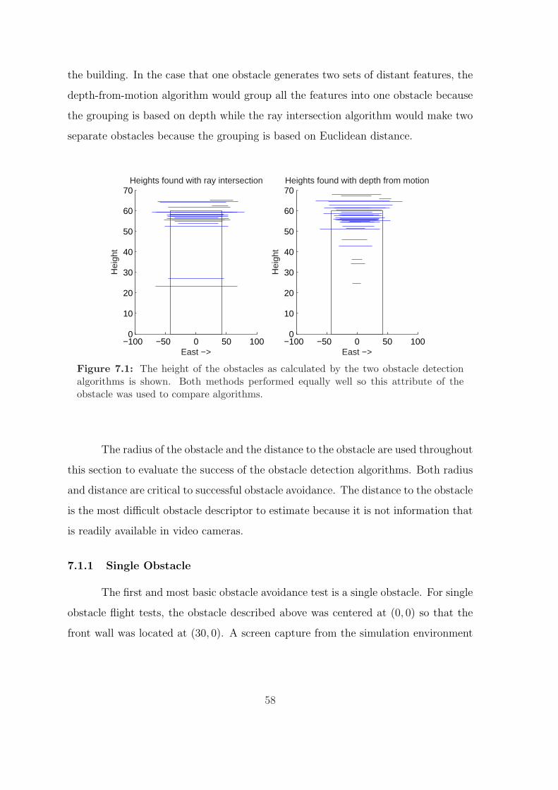
the building. In the case that one obstacle generates two sets of distant features, the
depth-from-motion algorithm would group all the features into one obstacle because
the grouping is based on depth while the ray intersection algorithm would make two
separate obstacles because the grouping is based on Euclidean distance.
−100 −50 0 50 1000
10
20
30
40
50
60
70
East −>
Hei
ght
Heights found with ray intersection
−100 −50 0 50 1000
10
20
30
40
50
60
70
East −>
Hei
ght
Heights found with depth from motion
Figure 7.1: The height of the obstacles as calculated by the two obstacle detectionalgorithms is shown. Both methods performed equally well so this attribute of theobstacle was used to compare algorithms.
The radius of the obstacle and the distance to the obstacle are used throughout
this section to evaluate the success of the obstacle detection algorithms. Both radius
and distance are critical to successful obstacle avoidance. The distance to the obstacle
is the most difficult obstacle descriptor to estimate because it is not information that
is readily available in video cameras.
7.1.1 Single Obstacle
The first and most basic obstacle avoidance test is a single obstacle. For single
obstacle flight tests, the obstacle described above was centered at (0, 0) so that the
front wall was located at (30, 0). A screen capture from the simulation environment
58
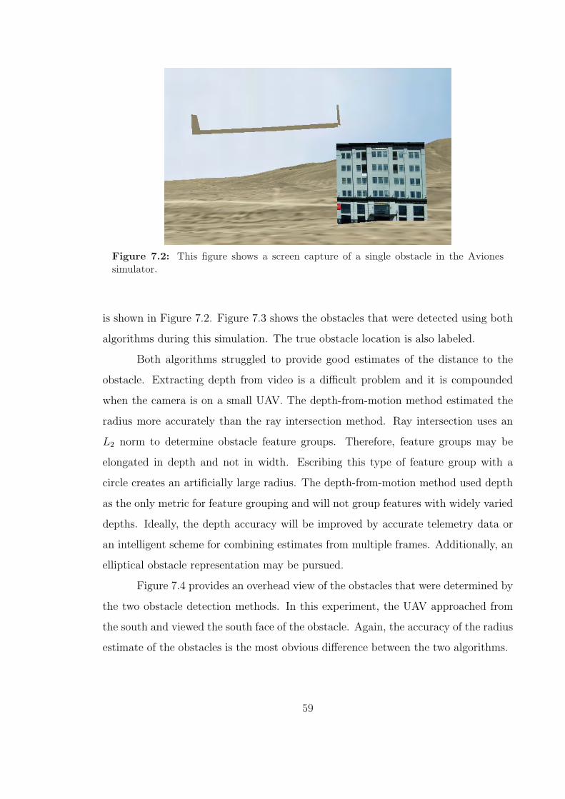
Figure 7.2: This figure shows a screen capture of a single obstacle in the Avionessimulator.
is shown in Figure 7.2. Figure 7.3 shows the obstacles that were detected using both
algorithms during this simulation. The true obstacle location is also labeled.
Both algorithms struggled to provide good estimates of the distance to the
obstacle. Extracting depth from video is a difficult problem and it is compounded
when the camera is on a small UAV. The depth-from-motion method estimated the
radius more accurately than the ray intersection method. Ray intersection uses an
L2 norm to determine obstacle feature groups. Therefore, feature groups may be
elongated in depth and not in width. Escribing this type of feature group with a
circle creates an artificially large radius. The depth-from-motion method used depth
as the only metric for feature grouping and will not group features with widely varied
depths. Ideally, the depth accuracy will be improved by accurate telemetry data or
an intelligent scheme for combining estimates from multiple frames. Additionally, an
elliptical obstacle representation may be pursued.
Figure 7.4 provides an overhead view of the obstacles that were determined by
the two obstacle detection methods. In this experiment, the UAV approached from
the south and viewed the south face of the obstacle. Again, the accuracy of the radius
estimate of the obstacles is the most obvious difference between the two algorithms.
59
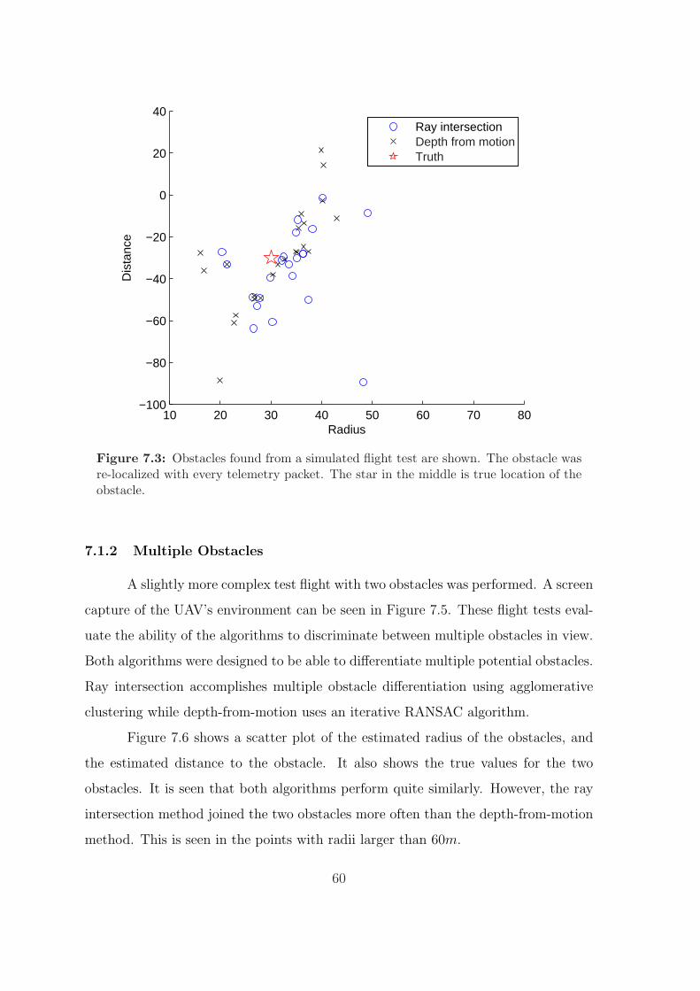
10 20 30 40 50 60 70 80−100
−80
−60
−40
−20
0
20
40
Radius
Dis
tanc
e
Ray intersectionDepth from motionTruth
Figure 7.3: Obstacles found from a simulated flight test are shown. The obstacle wasre-localized with every telemetry packet. The star in the middle is true location of theobstacle.
7.1.2 Multiple Obstacles
A slightly more complex test flight with two obstacles was performed. A screen
capture of the UAV’s environment can be seen in Figure 7.5. These flight tests eval-
uate the ability of the algorithms to discriminate between multiple obstacles in view.
Both algorithms were designed to be able to differentiate multiple potential obstacles.
Ray intersection accomplishes multiple obstacle differentiation using agglomerative
clustering while depth-from-motion uses an iterative RANSAC algorithm.
Figure 7.6 shows a scatter plot of the estimated radius of the obstacles, and
the estimated distance to the obstacle. It also shows the true values for the two
obstacles. It is seen that both algorithms perform quite similarly. However, the ray
intersection method joined the two obstacles more often than the depth-from-motion
method. This is seen in the points with radii larger than 60m.
60
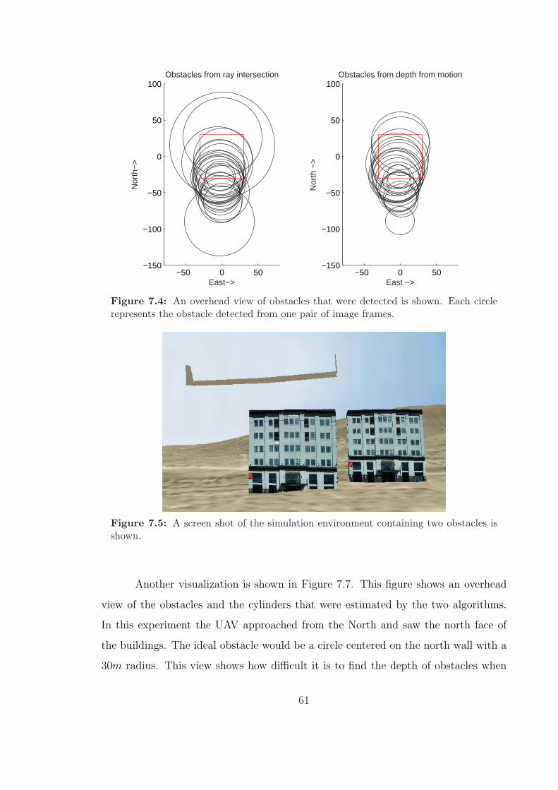
−50 0 50−150
−100
−50
0
50
100Obstacles from ray intersection
Nor
th−
>
East−>−50 0 50
−150
−100
−50
0
50
100Obstacles from depth from motion
Nor
th −
>
East −>
Figure 7.4: An overhead view of obstacles that were detected is shown. Each circlerepresents the obstacle detected from one pair of image frames.
Figure 7.5: A screen shot of the simulation environment containing two obstacles isshown.
Another visualization is shown in Figure 7.7. This figure shows an overhead
view of the obstacles and the cylinders that were estimated by the two algorithms.
In this experiment the UAV approached from the North and saw the north face of
the buildings. The ideal obstacle would be a circle centered on the north wall with a
30m radius. This view shows how difficult it is to find the depth of obstacles when
61
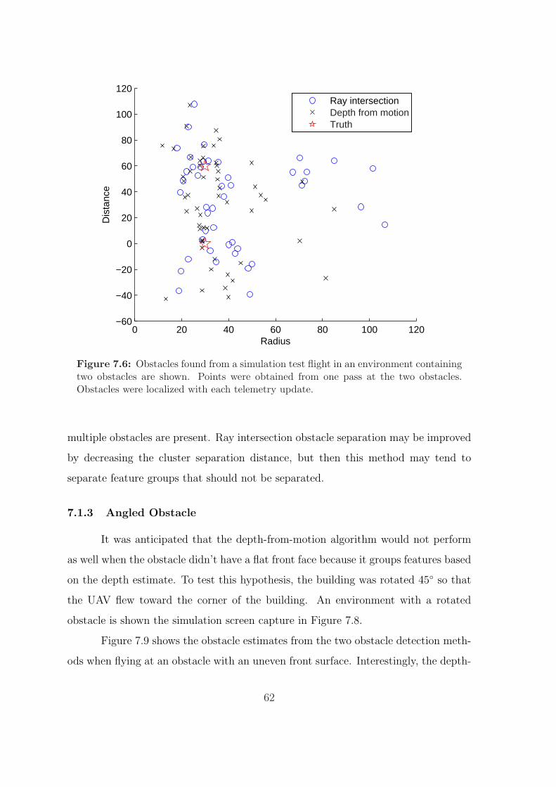
0 20 40 60 80 100 120−60
−40
−20
0
20
40
60
80
100
120
Radius
Dis
tanc
e
Ray intersectionDepth from motionTruth
Figure 7.6: Obstacles found from a simulation test flight in an environment containingtwo obstacles are shown. Points were obtained from one pass at the two obstacles.Obstacles were localized with each telemetry update.
multiple obstacles are present. Ray intersection obstacle separation may be improved
by decreasing the cluster separation distance, but then this method may tend to
separate feature groups that should not be separated.
7.1.3 Angled Obstacle
It was anticipated that the depth-from-motion algorithm would not perform
as well when the obstacle didn’t have a flat front face because it groups features based
on the depth estimate. To test this hypothesis, the building was rotated 45◦ so that
the UAV flew toward the corner of the building. An environment with a rotated
obstacle is shown the simulation screen capture in Figure 7.8.
Figure 7.9 shows the obstacle estimates from the two obstacle detection meth-
ods when flying at an obstacle with an uneven front surface. Interestingly, the depth-
62
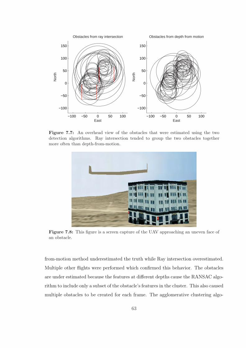
−100 −50 0 50 100
−100
−50
0
50
100
150
Obstacles from ray intersection
Nor
th
East−100 −50 0 50 100
−100
−50
0
50
100
150
Obstacles from depth from motion
Nor
th
East
Figure 7.7: An overhead view of the obstacles that were estimated using the twodetection algorithms. Ray intersection tended to group the two obstacles togethermore often than depth-from-motion.
Figure 7.8: This figure is a screen capture of the UAV approaching an uneven face ofan obstacle.
from-motion method underestimated the truth while Ray intersection overestimated.
Multiple other flights were performed which confirmed this behavior. The obstacles
are under estimated because the features at different depths cause the RANSAC algo-
rithm to include only a subset of the obstacle’s features in the cluster. This also caused
multiple obstacles to be created for each frame. The agglomerative clustering algo-
63
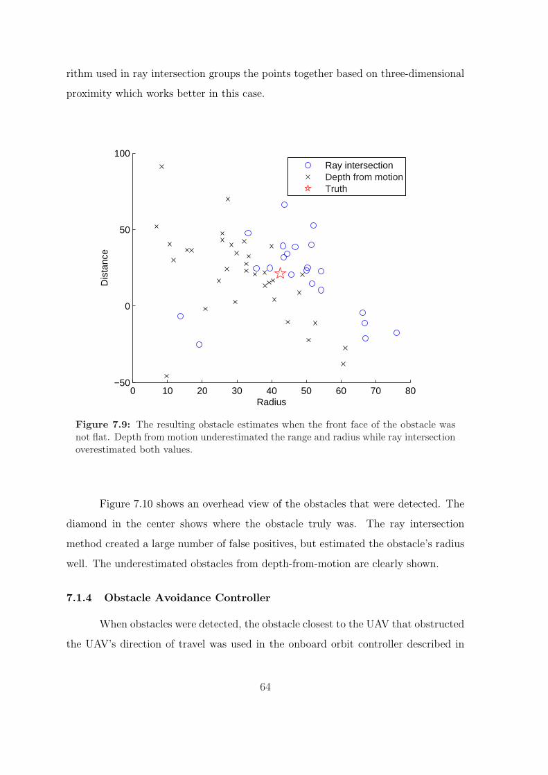
rithm used in ray intersection groups the points together based on three-dimensional
proximity which works better in this case.
0 10 20 30 40 50 60 70 80−50
0
50
100
Radius
Dis
tanc
e
Ray intersectionDepth from motionTruth
Figure 7.9: The resulting obstacle estimates when the front face of the obstacle wasnot flat. Depth from motion underestimated the range and radius while ray intersectionoverestimated both values.
Figure 7.10 shows an overhead view of the obstacles that were detected. The
diamond in the center shows where the obstacle truly was. The ray intersection
method created a large number of false positives, but estimated the obstacle’s radius
well. The underestimated obstacles from depth-from-motion are clearly shown.
7.1.4 Obstacle Avoidance Controller
When obstacles were detected, the obstacle closest to the UAV that obstructed
the UAV’s direction of travel was used in the onboard orbit controller described in
64
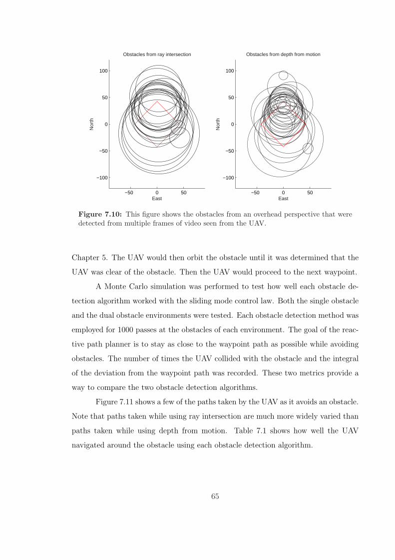
−50 0 50
−100
−50
0
50
100
Obstacles from ray intersection
Nor
th
East−50 0 50
−100
−50
0
50
100
Obstacles from depth from motion
Nor
th
East
Figure 7.10: This figure shows the obstacles from an overhead perspective that weredetected from multiple frames of video seen from the UAV.
Chapter 5. The UAV would then orbit the obstacle until it was determined that the
UAV was clear of the obstacle. Then the UAV would proceed to the next waypoint.
A Monte Carlo simulation was performed to test how well each obstacle de-
tection algorithm worked with the sliding mode control law. Both the single obstacle
and the dual obstacle environments were tested. Each obstacle detection method was
employed for 1000 passes at the obstacles of each environment. The goal of the reac-
tive path planner is to stay as close to the waypoint path as possible while avoiding
obstacles. The number of times the UAV collided with the obstacle and the integral
of the deviation from the waypoint path was recorded. These two metrics provide a
way to compare the two obstacle detection algorithms.
Figure 7.11 shows a few of the paths taken by the UAV as it avoids an obstacle.
Note that paths taken while using ray intersection are much more widely varied than
paths taken while using depth from motion. Table 7.1 shows how well the UAV
navigated around the obstacle using each obstacle detection algorithm.
65
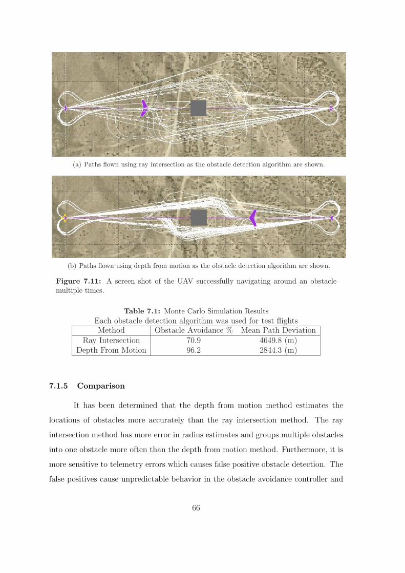
(a) Paths flown using ray intersection as the obstacle detection algorithm are shown.
(b) Paths flown using depth from motion as the obstacle detection algorithm are shown.
Figure 7.11: A screen shot of the UAV successfully navigating around an obstaclemultiple times.
Table 7.1: Monte Carlo Simulation ResultsEach obstacle detection algorithm was used for test flightsMethod Obstacle Avoidance % Mean Path Deviation
Ray Intersection 70.9 4649.8 (m)Depth From Motion 96.2 2844.3 (m)
7.1.5 Comparison
It has been determined that the depth from motion method estimates the
locations of obstacles more accurately than the ray intersection method. The ray
intersection method has more error in radius estimates and groups multiple obstacles
into one obstacle more often than the depth from motion method. Furthermore, it is
more sensitive to telemetry errors which causes false positive obstacle detection. The
false positives cause unpredictable behavior in the obstacle avoidance controller and
66
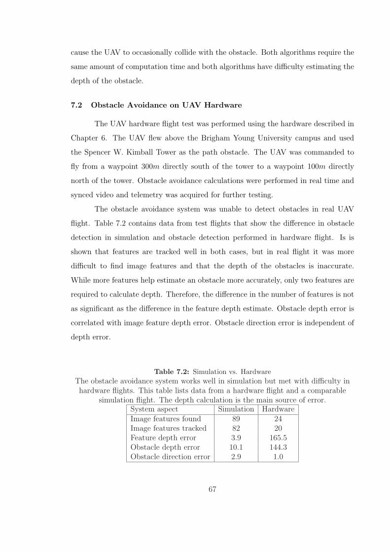
cause the UAV to occasionally collide with the obstacle. Both algorithms require the
same amount of computation time and both algorithms have difficulty estimating the
depth of the obstacle.
7.2 Obstacle Avoidance on UAV Hardware
The UAV hardware flight test was performed using the hardware described in
Chapter 6. The UAV flew above the Brigham Young University campus and used
the Spencer W. Kimball Tower as the path obstacle. The UAV was commanded to
fly from a waypoint 300m directly south of the tower to a waypoint 100m directly
north of the tower. Obstacle avoidance calculations were performed in real time and
synced video and telemetry was acquired for further testing.
The obstacle avoidance system was unable to detect obstacles in real UAV
flight. Table 7.2 contains data from test flights that show the difference in obstacle
detection in simulation and obstacle detection performed in hardware flight. Is is
shown that features are tracked well in both cases, but in real flight it was more
difficult to find image features and that the depth of the obstacles is inaccurate.
While more features help estimate an obstacle more accurately, only two features are
required to calculate depth. Therefore, the difference in the number of features is not
as significant as the difference in the feature depth estimate. Obstacle depth error is
correlated with image feature depth error. Obstacle direction error is independent of
depth error.
Table 7.2: Simulation vs. HardwareThe obstacle avoidance system works well in simulation but met with difficulty inhardware flights. This table lists data from a hardware flight and a comparable
simulation flight. The depth calculation is the main source of error.System aspect Simulation HardwareImage features found 89 24Image features tracked 82 20Feature depth error 3.9 165.5Obstacle depth error 10.1 144.3Obstacle direction error 2.9 1.0
67
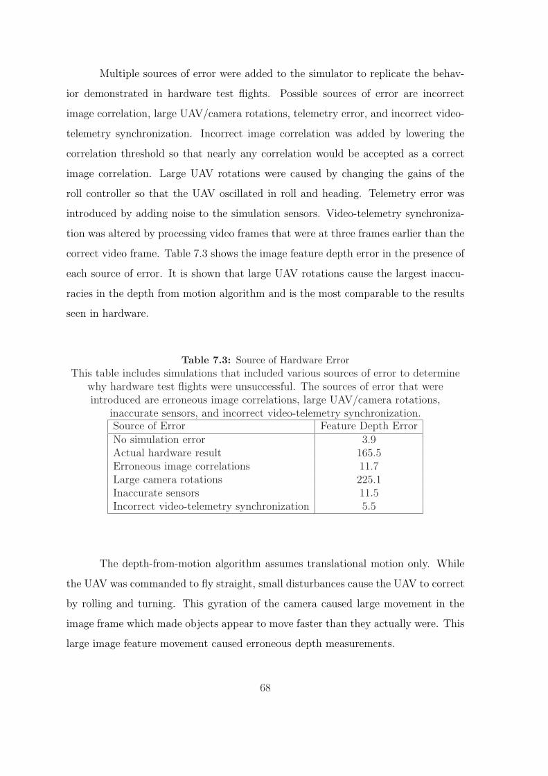
Multiple sources of error were added to the simulator to replicate the behav-
ior demonstrated in hardware test flights. Possible sources of error are incorrect
image correlation, large UAV/camera rotations, telemetry error, and incorrect video-
telemetry synchronization. Incorrect image correlation was added by lowering the
correlation threshold so that nearly any correlation would be accepted as a correct
image correlation. Large UAV rotations were caused by changing the gains of the
roll controller so that the UAV oscillated in roll and heading. Telemetry error was
introduced by adding noise to the simulation sensors. Video-telemetry synchroniza-
tion was altered by processing video frames that were at three frames earlier than the
correct video frame. Table 7.3 shows the image feature depth error in the presence of
each source of error. It is shown that large UAV rotations cause the largest inaccu-
racies in the depth from motion algorithm and is the most comparable to the results
seen in hardware.
Table 7.3: Source of Hardware ErrorThis table includes simulations that included various sources of error to determine
why hardware test flights were unsuccessful. The sources of error that wereintroduced are erroneous image correlations, large UAV/camera rotations,
inaccurate sensors, and incorrect video-telemetry synchronization.Source of Error Feature Depth ErrorNo simulation error 3.9Actual hardware result 165.5Erroneous image correlations 11.7Large camera rotations 225.1Inaccurate sensors 11.5Incorrect video-telemetry synchronization 5.5
The depth-from-motion algorithm assumes translational motion only. While
the UAV was commanded to fly straight, small disturbances cause the UAV to correct
by rolling and turning. This gyration of the camera caused large movement in the
image frame which made objects appear to move faster than they actually were. This
large image feature movement caused erroneous depth measurements.
68
To create a system that successfully avoids obstacles on a small UAV the
motions of the UAV must be separated into translation and rotation and the feature
movement from rotation must be removed before calculating depth. Separating the
rotational movement from the translational movement can be done in two ways.
First, the telemetry of the UAV may be used to find the rotation. However, it has
been observed that the telemetry is not accurate enough to be successfully used in
other algorithms such as ray intersection. Second, the telemetry of the UAV can be
estimated using the computer-vision fundamental matrix. This matrix maps points
from a first camera coordinate to a second camera coordinate and can be found using
image feature tracking.
7.3 Summary
This chapter contains results from multiple simulations and hardware flight
tests. A simulated UAV correctly detected obstacles in environments with one obsta-
cle, two obstacles, and an uneven-faced obstacle. The depth-from-motion algorithm
estimated the single obstacle and the multiple obstacles more accurately than ray
intersection, but detected the uneven obstacle poorly. A Monte Carlo simulation was
performed where each obstacle detection algorithm was used to detect obstacles for
navigation. The ray intersection algorithm was able to avoid obstacles 70% success-
fully while the depth-from-motion algorithm was able to avoid obstacles 90% success-
fully. Finally, hardware test flights were performed and evaluated. Neither obstacle
detection method was successful in hardware test flights, but additional simulations
were executed testing various sources of error. It was shown that large rotations of
the UAV caused inaccuracies similar to the error seen from hardware test flights.
69

70
Chapter 8
Conclusion
This research contributes a novel approach for obstacle avoidance for small
UAV’s using computer vision to the body of scientific knowledge. Small UAV’s require
a light weight, low cost and highly mobile obstacle avoidance solution. The system
presented here uses a video camera to sense the environment, calculates depth from
video motion, localizes potential hazards, and successfully navigates around them.
The obstacle avoidance system is developed for small UAV hardware such as
the hardware described in Chapter 6. Known obstacles are avoided using a genetic
algorithm pre-mission path planner. Then the system employs a small, fixed, forward-
looking camera which transmits video to a mobile ground station to detect and avoid
obstacles. The video is searched for image features using the Harris Corner Detector,
and image features are tracked through multiple frames using image correlation. The
depth of the image features is determined using feature movement and known UAV
movement. The features are localized in world coordinates using depth from motion
equations. Features are grouped with other nearby features using RANSAC to create
potential hazardous areas. These areas are represented using bounding cylinders and
avoided using a sliding mode orbit controller.
This system avoids up to 96% of obstacles in simulation and is evaluated in
hardware test flights. As currently implemented, the system does not work in hard-
ware because the UAV’s attitude cannot be detected accurately using small sensors.
The attitude of the UAV may be estimated using computer vision by finding the
fundamental matrix (F ). This matrix is estimated using the RANSAC method and
image feature tracking. However, much of the video is comprised of sky, distant
mountains and trees which tend to have very few image corners. The bottom half of
71
the image often contains sparse, man-made structures which provide some features.
However, the fundamental matrix is difficult to estimate with few features. A more
downward-oriented camera would find more features, but not be as capable of seeing
obstacles in front of the UAV. In order to perform obstacle avoidance on small UAVs,
the attitude of the UAV must be more accurately estimated.
8.1 Future Work
Multiple improvements can be made to the research presented in this the-
sis. The main target of future research is to improve the rate of successful obstacle
avoidance for real UAV’s. Future work can be grouped into two main areas: obsta-
cle estimation and obstacle avoidance controller. Obstacle estimation includes using
more accurate depth from video algorithms, representing obstacles in new ways, and
using obstacle information from multiple video frames to estimate the obstacle. The
obstacle avoidance controller can be improved by adding the ability to avoid multiple
obstacles and the ability to climb over obstacles.
One way to improve obstacle estimation is to use more accurate computer
vision algorithms to find the depth of the image. Ideally, the telemetry of the UAV
would be perfect and reliable, but in practice it is difficult and expensive to estimate
the UAV’s attitude accurately enough to heavily relied on for computer vision. Con-
versely, the video can be used to estimate the telemetry of the UAV using the video’s
fundamental matrix. However, this estimate may also be inaccurate. Future research
can evaluate combining telemetry from sensors and video in a way that may help the
accuracy of obstacle estimation.
A second way to improve obstacle estimation is to represent obstacles using
ellipses or planar surfaces. Alternate representations would allow the obstacle to be
represented more accurately. The depth from motion method assumes that all fea-
tures that are grouped together are the same distance from the UAV. This assumption
leads logically to representing the obstacle using planar surfaces. The difficulty in us-
ing this representation is that a different control law would be required. The RRT
discussed in Section 2.1 is capable of handling planar representations. Another alter-
72
nate representation is an elliptical cylinder. An ellipse can more accurately represent
an obstacle that is oblong. Furthermore, the sliding mode control law would need
minor modifications to navigate this alternate representation.
A third way to improve obstacle estimation is to combine the information ac-
cumulated from multiple video frames into one obstacle estimate. The current system
uses the obstacle detected from one frame and navigates around it. Combining ob-
stacles from multiple frames would allow for more accurate obstacle estimation. The
information could be combined using a filtering or averaging method. The difficulty
is that multiple obstacles may be detected or one obstacle may be represented as
multiple obstacles. One obstacles from a first frame may need to be separated into
two obstacles or two obstacles from one frame may need to be combined into one. A
further complication is introduced when the confidence in an obstacle measurement
is incorporated. Using information from multiple successive frames is not trivial, but
is potentially very useful for obstacle avoidance.
The obstacle avoidance controller can be improved by keeping a map of all
the obstacles that are detected and avoiding all obstacles at the same time. This is a
natural next step from using obstacle information from multiple frames because the
map will be the current estimates of obstacles and the confidence in the estimation of
obstacles will be much higher. A modified sliding mode controller may be evaluated
for multiple obstacle avoidance or a different controller may be implemented.
Finally it would be desirable to evaluate the use of different controllers that
have the capability to navigate over the obstacle as well as around it. Vertical nav-
igation gives the UAV the ability to be more efficient if it is determined that flying
over an obstacle could save energy. A new rule could be added to the sliding mode
controller that command the UAV to navigate over the obstacle, or a different con-
troller could be implemented. The rapidly exploring random tree algorithm discussed
in Section 2.1 is a good path planner that is both computationally fast and has the
ability to fly around multiple obstacles or navigate over them.
73

74
Bibliography
[1] T. Schouwenaars, J. How, and E. Feron, “Receeding horizon path planning withimplicit safety guarantees,” in Proceedings of the 2004 American Control Con-ference, vol. 6, July 2004, pp. 5576–5581. 3
[2] Z. Sun, D. Hsu, T. Jiang, H. Kurniawati, and J. H. Reif, “Narrow passagesampling for probabilistic roadmap planning,” IEEE Transactions on Robotics,vol. 21, no. 6, pp. 1105–1115, December 2005. 3
[3] B. Sinopoli, M. Micheli, G. Donato, and T. J. Koo, “Vision based navigationfor an unmanned aerial vehicle,” Proceedings of the International Conference onRobotics and Automation, vol. 2, pp. 1757–1764, May 2001. 3
[4] D. K. Pai and L.-M. Reissell, “Multiresolution rough terrain motion planning,”in IEEE Transactions on Robotics and Automation, vol. 14, no. 1, Februaruy1998, pp. 19–33. 3
[5] D. Rathbun and B. Capozzi, “Evolutionary approaches to path planningthrough uncertain environments,” in 1st UAV Conference, no. AIAA 2002-3455,Portsmouth, Virginia, May 20–23 2002. 3, 7
[6] S. A. Bartoff, “Path planning for UAVs,” in Proceedings of the American ControlConference, vol. 1, no. 6, Chicago, Illinois, September 2000, pp. 364–368. 3, 7
[7] J. B. Saunders, B. Call, A. Curtis, R. W. Beard, and T. W. McLain, “Staticand dynamic obstacle avoidance in miniature air vehicles,” in AIAA Infotech atAerospace, 2005, paper no. AIAA-2005-6950. 4
[8] K. Sabe, M. Fukuchi, J.-S. Gutmann, T. Ohashi, K. Kawamoto, and T. Yoshiga-hara, “Obstacle avoidance and path planning for humanoid robots using stereovision,” in Proceedings of the International Conference on Robotics and Automa-tion, vol. 1, April 2004, pp. 592–597. 4
[9] S. Badal, S. Ravela, B. Draper, and A. Hanson, “A practical obstacle detectionand avoidance system,” in Proceedings of the Second IEEE Workshop on Appli-cations of Computer Vision, ser. 2nd, Sarasota, FL, USA, December 1994, pp.97–104. 4
[10] R. M. Bolle and B. C. Vemuri, “On three-dimensional surface reconstructionmethods,” IEEE Transactions on Pattern Analysis and Machine Intelligence,vol. 13, no. 1, pp. 1–13, January 1991. 4
75
[11] D. Coombs, M. Herman, T.-H. Hong, and M. Nashman, “Real-time obstacleavoidance using central flow divergence, and peripheral flow,” in IEEE Trans-actions on Robotics and Automation, vol. 14, no. 1, February 1998, pp. 49–59.4
[12] J. Huber and V. Graefe, “Motion stereo for mobile robots,” IEEE Transactionson Industrial Electronics, vol. 41, no. 4, pp. 378–383, Aug 1994. 4, 39
[13] W. H. Huang, B. R. Fajen, J. R. Fink, and W. H. Warren, “Visual naviga-tion and obstacle avoidance using steering potential function,” in Robotics andAutonomous Systems, vol. 54, November 2006, pp. 288–299. 7, 51
[14] P. Cheng, Z. Shen, and S. M. LaValle, “RRT-based trajectory design for au-tonomous automobiles and spacecraft,” Archives of Control Sciences, vol. 11,no. 3-4, pp. 167–194, 2001. 7, 9
[15] S. M. LaValle, “Rapidly-exploring random trees: A new tool for path planning,”Computer Science Dept., Iowa State University, Tech. Rep. TR 98-11, 1998. 8
[16] ——, “The rapidly-exploring random tree (RRT) page,” http://msl.cs.uiuc.edu/rrt, August 2006. 8
[17] J. Holland, Adaptation in natural and artificial systems. MIT Press Cambridge,MA, USA, 1992. 11
[18] Wikipedia, “Genetic algorithm applications,” http://en.wikipedia.org/wiki/Genetic algorithm, August 2006. 11
[19] H. P. Moravec, “Towards automatic visual obstacle avoidance,” in The Interna-tional Joint Conference on Artificial Intelligence, 1977, p. 584. 22
[20] L. Kitchen and A. Rosenfeld, “Gray-level corner detection,” Pattern RecognitionLetters, vol. 1, no. 2, pp. 95–102, December 1982. 22
[21] C. J. Harris and M. Stephens, “A combined corner and edge detector,” In Proc.4th Alvey Vision Conf. , Manchester, pp. 147–151, 1988. 22, 23
[22] S. M. Smith, “A new class of corner finder,” in 3rd British Machine VisionConference, 1992, pp. 139–148. 22
[23] F. Mokhtarian and R. Suomela, “Robust image corner detection through curva-ture scale space,” IEEE Transaction on Pattern Analysis and Machine Intelli-gence, vol. 20, no. 12, pp. 1376 – 1381, December 1998. 22, 23
[24] Intel, “Open source computer vision library,” http://www.intel.com/technology/computing/opencv/index.htm, August 2006. 23
[25] H. Moravec, “Obstacle avoidance and navigation in the real world by a seeingrobot rover,” Ph.D. dissertation, Stanford Univerisity, May 1980. 25
76
[26] A. M. Eldredge, “Improved state estimation for miniature air vehicles,” Master’sthesis, Brigham Young University, 2006. 31
[27] E. W. Weisstein, “Mathworld,” From MathWorld – A Wolfram Web Resourcehttp://mathworld.wolfram.com, August 2006. 31
[28] J. Redding, “Vision-based target localization from a small, fixed-wing unmannedair vehicle,” Master’s thesis, Brigham Young University, 459 Clyde Building,Provo, UT 84604, 2005. 31
[29] J. A. Hartigan and M. A. Wong, “Algorithm AS136, a k-means clustering algo-rithm,” Statistical algorithms, vol. 28, no. 1, pp. 100–108, 1979. 36
[30] A. Baraldi and P. Blonda, “A survey of fuzzy clustering algoirthms for patternrecognition - part II,” in IEEE Transactions on Systems, Man, and Cybernetics– Part B: Cybernetics, vol. 29, no. 6, December 1999, pp. 786 – 801. 36
[31] C. Ding and X. He, “Cluster merging and splitting in hierarchical clusteringalgorithms,” Proceedings of the IEEE International Conference on Data Mining(ICDM’02), pp. 139–146, 2002. 36
[32] M. A. Fischler and R. C. Bolles, “Random sample consensus: A paradigm formodel fitting with applications to image analysis and automated cartography,”in Communications of the ACM, vol. 24, June 1981, pp. 381–395. 41
[33] R. Hartley and A. Zisserman, Multiple View Geometry in Computer Vision,2nd ed. Cambridge University Press, March 2004. 41
[34] D. R. Nelson, D. B. Barber, T. W. McLain, and R. Beard, “Vector field path fol-lowing for small unmanned air vehicles,” in Proceedings of the American ControlConference, June 2006, pp. 5788–5794. 47
[35] Unicorn-Wings, “Unicorn wings,” http://unicornwings.stores.yahoo.net/, Au-gust 2006. 55
[36] Procerus, “Procerus technologoies: Fly light with the world’s smallest uav au-topilot,” http://www.procerusuav.com/, August 2006. 55
[37] Furuno, “Furuno marine electronics,” http://www.furuno.com/, August 2006.55
[38] Black-Widow-Aerial-Video, “Wireless video equipment for ground and aerielwork,” http://www.blackwidowav.com/, August 2006. 55
[39] Imperx, “Imperx incorporated,” http://www.imperx.com/, August 2006. 55
[40] Hewlett-Packard, “HP united states - computers, laptops, servers, printers &more,” http://www.hp.com, August 2006. 55
[41] D. Hearn and M. P. Baker, Computer Graphics with OpenGL, 3rd ed., M. J.Horton, Ed. Pearson Prentice Hall, 2004. 84
77

78
Appendix A
Random City Maker
A.1 Introduction
The Brigham Young University (BYU) Multiple Agent Intelligent Coordina-
tion and Control (MAGICC) research lab researches many aspects of small unmanned
air vehicles (UAV). Some of the research projects currently under development are
video stabilization, video mosaicing, obstacle avoidance, path planning, fire surveil-
lance, convoy surveillance, road following, multiple video stream use, multiple vehicle
coordination, multiple vehicle user interface, attitude estimation, and adaptive con-
trollers for small UAVs. To facilitate this research, students have created a UAV
simulator called Aviones. In order to increase the capability of Aviones to simulate
an urban environment, the ability to draw buildings, streets and vehicles has been
added. This document outlines how cities are created and how a researcher can use
them in conjunction with Aviones and provides implementation details about the
Random City Generator program.
The random city generator was initially began as a project for ME 570 -
Computer-Aided Engineering Software. This project was chosen because it was de-
sirable for both path planning and computer vision research. The cities created by the
random city generator can be loaded by the path planner and used for path planning
as well as loaded into Avoines and displayed in the environment.
This program was created using C++ and the Trolltech Qt graphical user
interface library. The program was compiled using Microsoft Visual Studio .net 2003,
but could be compiled on any compiler that Qt supports including gcc and Borland.
79
This documentation assumes that the reader is familiar with C++, Qt and object
oriented programming.
A.2 How to Create and Use Cities
Cities are created using the Random City Maker program. This program was
written using the Qt user interface library (version 3.2.0 Educational) and has been
compiled for Microsoft Windows. The Random City Maker creates a city with blocks
and streets in a spoke wheel layout and textures the city buildings with photos of real
world buildings. The city is saved as an xml file with a *.cit extension. This section
describes how to use the Random City Maker application to create cities that can be
used in Aviones and the Path Planner.
A.2.1 The Random City Maker User Interface
The user interface for the Random City Maker is a dockable window environ-
ment. Dockable windows give the user the ability to configure the user interface in a
way that works the best for the user. The windows that can be docked are
• City Properties - a window containing the variables that can be tuned when
creating random cities.
• Overhead view - a window displaying the overhead view of the city with North
upward. This window is used to select buildings.
• Building Properties - a window containing the properties of the currently
selected building.
• Music Controls - a window that can be used to play music while you create
cities. This was added as a joke for the ME 570 teacher. It demonstrates how
easy Qt is to use because this entire widget took only a couple of hours to code
and debug.
80
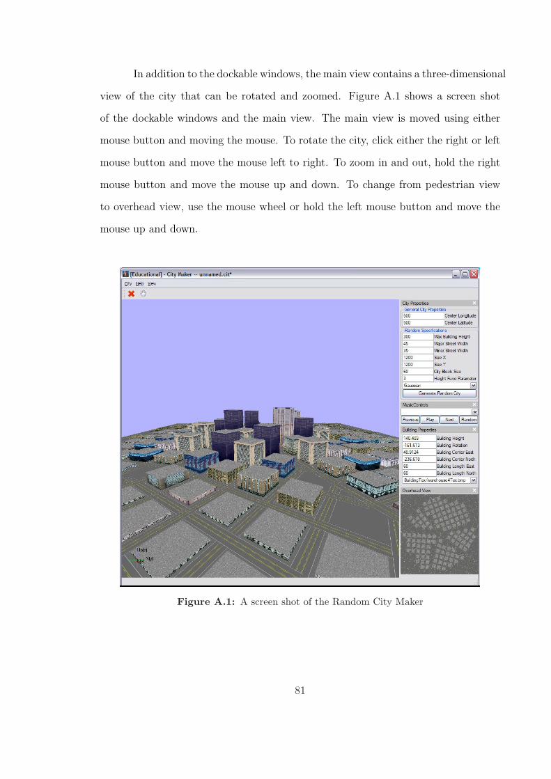
In addition to the dockable windows, the main view contains a three-dimensional
view of the city that can be rotated and zoomed. Figure A.1 shows a screen shot
of the dockable windows and the main view. The main view is moved using either
mouse button and moving the mouse. To rotate the city, click either the right or left
mouse button and move the mouse left to right. To zoom in and out, hold the right
mouse button and move the mouse up and down. To change from pedestrian view
to overhead view, use the mouse wheel or hold the left mouse button and move the
mouse up and down.
Figure A.1: A screen shot of the Random City Maker
81
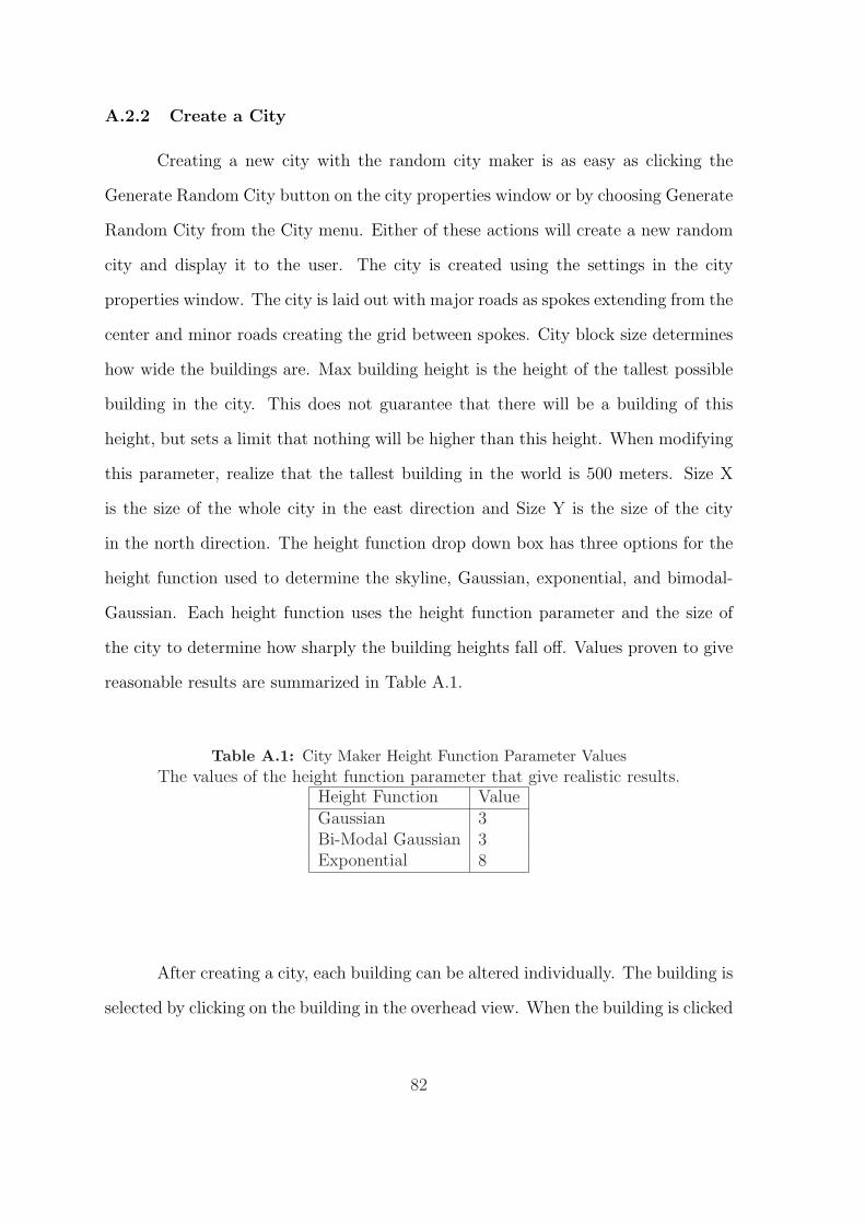
A.2.2 Create a City
Creating a new city with the random city maker is as easy as clicking the
Generate Random City button on the city properties window or by choosing Generate
Random City from the City menu. Either of these actions will create a new random
city and display it to the user. The city is created using the settings in the city
properties window. The city is laid out with major roads as spokes extending from the
center and minor roads creating the grid between spokes. City block size determines
how wide the buildings are. Max building height is the height of the tallest possible
building in the city. This does not guarantee that there will be a building of this
height, but sets a limit that nothing will be higher than this height. When modifying
this parameter, realize that the tallest building in the world is 500 meters. Size X
is the size of the whole city in the east direction and Size Y is the size of the city
in the north direction. The height function drop down box has three options for the
height function used to determine the skyline, Gaussian, exponential, and bimodal-
Gaussian. Each height function uses the height function parameter and the size of
the city to determine how sharply the building heights fall off. Values proven to give
reasonable results are summarized in Table A.1.
Table A.1: City Maker Height Function Parameter ValuesThe values of the height function parameter that give realistic results.
Height Function ValueGaussian 3Bi-Modal Gaussian 3Exponential 8
After creating a city, each building can be altered individually. The building is
selected by clicking on the building in the overhead view. When the building is clicked
82
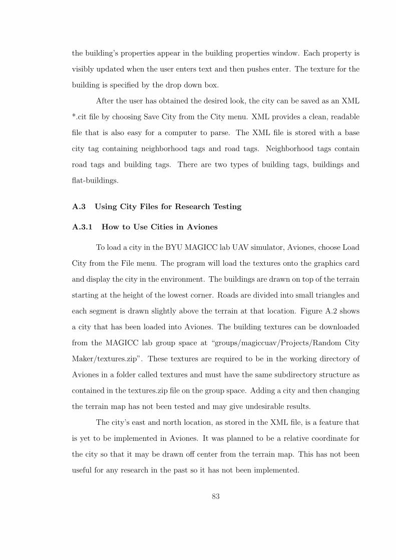
the building’s properties appear in the building properties window. Each property is
visibly updated when the user enters text and then pushes enter. The texture for the
building is specified by the drop down box.
After the user has obtained the desired look, the city can be saved as an XML
*.cit file by choosing Save City from the City menu. XML provides a clean, readable
file that is also easy for a computer to parse. The XML file is stored with a base
city tag containing neighborhood tags and road tags. Neighborhood tags contain
road tags and building tags. There are two types of building tags, buildings and
flat-buildings.
A.3 Using City Files for Research Testing
A.3.1 How to Use Cities in Aviones
To load a city in the BYU MAGICC lab UAV simulator, Aviones, choose Load
City from the File menu. The program will load the textures onto the graphics card
and display the city in the environment. The buildings are drawn on top of the terrain
starting at the height of the lowest corner. Roads are divided into small triangles and
each segment is drawn slightly above the terrain at that location. Figure A.2 shows
a city that has been loaded into Aviones. The building textures can be downloaded
from the MAGICC lab group space at “groups/magiccuav/Projects/Random City
Maker/textures.zip”. These textures are required to be in the working directory of
Aviones in a folder called textures and must have the same subdirectory structure as
contained in the textures.zip file on the group space. Adding a city and then changing
the terrain map has not been tested and may give undesirable results.
The city’s east and north location, as stored in the XML file, is a feature that
is yet to be implemented in Aviones. It was planned to be a relative coordinate for
the city so that it may be drawn off center from the terrain map. This has not been
useful for any research in the past so it has not been implemented.
83
Figure A.2: A screen shot of a city loaded into the simulator Aviones and drawn ontop of a real terrain model.
A.3.2 How to Use Cities in the Path Planner
City XML files can also be used in the MAGICC lab path planner software.
To add a city to the path planner, a terrain map must be loaded first. To load a
terrain, click the browse button and choose the terrain map file (*.tmf). When the
terrain maps are loaded, they are downsampled using the resolution in the terrain
resolution drop down box so that there will be enough resolution to add a detailed
city. To add the city after the terrain is loaded click the add city button and choose
the *.cit file. The four corners of each building in the city file are converted to four
terrain map coordinate corners using the terrain dimensions and scaling and the size
and rotation of the building. Then the height of the building is added to the terrain
inside the building corners using a polygon fill and a line drawing technique from
Computer Graphics with OpenGL [41].
A.4 City Generation Algorithm and Implementation
The random city maker generates a city in a spoke and wheel pattern and
fills in city segments with city block grids. Building height is determined using one
84
of three height functions. This section describes the algorithm for generating these
random cities.
A.4.1 Internal C++ Classes
The Random City uses the C++ class structure to organize the code. The
classes can be combined into two categories, user interface classes and object classes.
The user interface classes define how the user interacts with the program and are as
follows.
• CityDisplayGL - The openGL widget that displays the three dimensional view
of the city
• OverheadGL - The openGL widget that displays the overhead view of the city
• CityProperties - The window that contains the properties of the city
• BuildingProperties - The window that contains the properties of the default
buildings
• FlatBuildingProperties - The window that contains the properties of the flat
block textures
• MusicControls - The completely unnecessary music player user interface
The non-openGL user interface widgets are easily modified using Qt Designer, a user
interface for creating dialogs and widgets.
Object classes are classes that define the physical structures. Each class con-
tains information about location, size and description of the object. Each class knows
how to render itself in an openGL context and how to read itself from an XML file.
• BCity - A class containing city attributes
85
• BNeighborhood - A class that records the polygon outline of a neighborhood
and manages the buildings and roads within that neighborhood
• BBuilding - A base class that has default behavior to draw a textured building
in the given block
• BBuildingFlat - A class that inherits from BBuilding and draws a flat texture
on a block instead of a tall building
• BBuildingTex - A class that contains a building texture and an associated
acceptable height range for that texture
• BRoad - A class that can load one of two different textures depending on if it
is a major road or a minor road
Lastly, the program uses tinyXML which is a small XML library that was
downloaded and used to read XML files.
A.4.2 City Generation Algorithm
When the Generate Random City button is pressed, the BCity::createRandom()
function gets called which in turn calls BCity::createRandomBuildings(). The cre-
ateRandomBuildings() function divides the city area rectangle radially by randomly
generating main roads. Main roads are described by their angle measured in degrees
on the set [−180, 180]. The angle of the first road is selected randomly between
[−180,−90]. Subsequent angles are determined by adding a random value from the
set [30, 120] to the previous angle as seen in red in Figure A.3. If the previous an-
gle plus 120 is larger than 180 then the the random number is chosen from the set
[prevAngle + 30, 180] and the program stops generating roads.
Neighborhoods are defined as the area between main roads and inside the
city boundaries. Neighborhoods are represented by a list of points comprising a
86
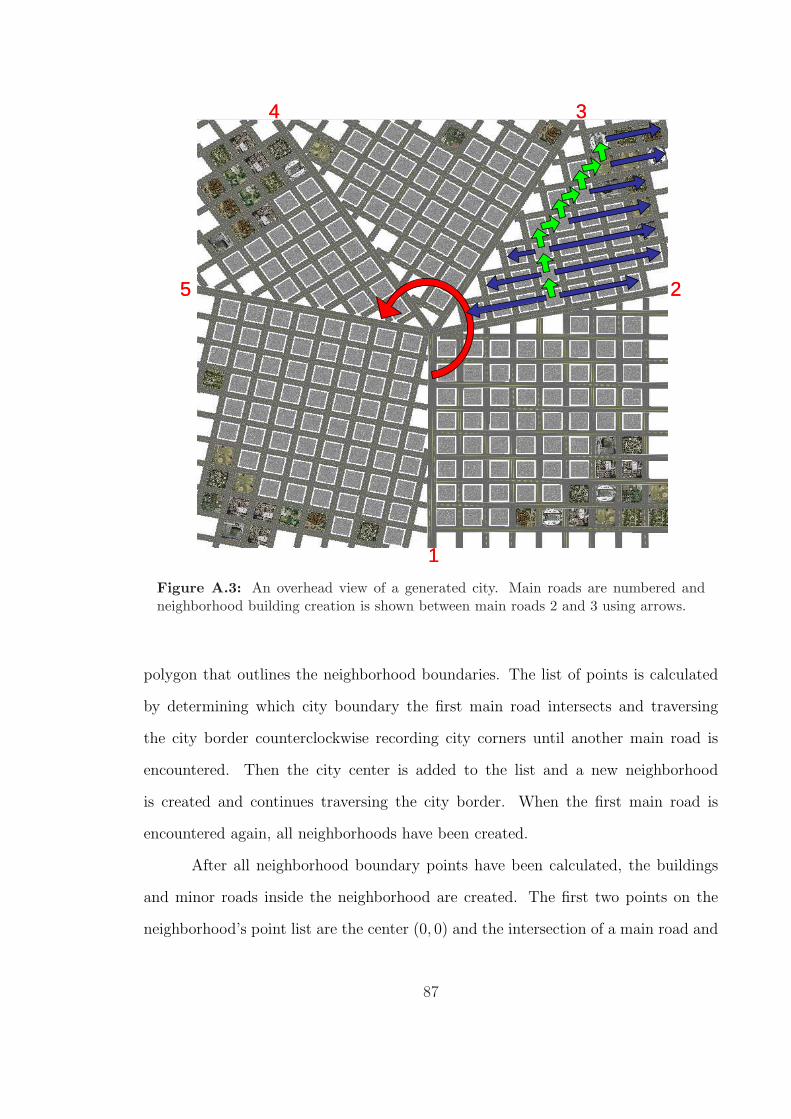
1
2
34
5
1
2
34
5
Figure A.3: An overhead view of a generated city. Main roads are numbered andneighborhood building creation is shown between main roads 2 and 3 using arrows.
polygon that outlines the neighborhood boundaries. The list of points is calculated
by determining which city boundary the first main road intersects and traversing
the city border counterclockwise recording city corners until another main road is
encountered. Then the city center is added to the list and a new neighborhood
is created and continues traversing the city border. When the first main road is
encountered again, all neighborhoods have been created.
After all neighborhood boundary points have been calculated, the buildings
and minor roads inside the neighborhood are created. The first two points on the
neighborhood’s point list are the center (0, 0) and the intersection of a main road and
87
the city border. The building grid for the neighborhood is aligned parallel with this
first main road. The first building is placed between the center of the city and the
edge of the city along this first main road. Then the streets that are perpendicular to
this main road are incrementally placed while the streets are inside the neighborhood.
The streets that are parallel to the main street are placed in the same fashion.
Next, the buildings are placed in the neighborhood. First, buildings are placed
along the first main road to the right and to the left of the first building. Then a
new row is created by starting from the location of the first building and stepping
away from the main road. If this new location is inside the neighborhood, a new row
of buildings is created. If this new location is outside the neighborhood then five
blocks to the right or left are checked to see if they are in the neighborhood. The first
block entirely inside the neighborhood is used as the new row center block. Building
creation is shown in Figure A.3 between main roads 2 and 3. If no such block can
be found, then the neighborhood is complete. The rotation of each building is the
angle of the main road and the height of the building is calculated as described in
Section A.4.3
A.4.3 Height Functions
The user may specify one of three height functions for the buildings that
are created. Three height functions are available because most actual cities have a
Gaussian distribution, but some cities with a few tall buildings look more exponential,
and others where two cities have grown together, have a bi-modal Gaussian height
function. Examples of the three height functions in the Random City Maker can be
seen in Figure A.4 In each case, the height of any location is computed, then the
height is decreased by a random percentage of the original height chosen from the
set [0%, 70%]. If the height function returns a value less than 10m, a flat building
texture is used for that block.
88
In the following height functions, h is the height returned for the building,
hmax is the maximum height for any building, (x, y) is the location of the building
in the city, (cx, cy) is the size of the city in each dimension, (sx, sy) is the horizontal
shift of the distribution and v is a user specified height decay value. The bivariate
normal distribution,
h = hmax ∗ 1
2πσxσy
√1− ρ2
e− z
2(1−ρ2) , (A.1)
(A.2)
was used to calculate the Gaussian height function where
z =(x− sx)
2
σ2x
− 2ρ(x− sx)(y − sy)
σxσy
+(y − sy)
2
σ2y
,
σx =cx
v,
σy =cy
v.
For Gaussian distribution calculations, ρ is set to 0.1. Figure A.4.3 provides a graph-
ical representation of Equation A.1. The exponential function is
h = hmaxe−q
vcx∗cy
(x2+y2), (A.3)
which creates a circular exponential cone as seen in Figure A.4.3. Values for v that
produce good height decay for each height function are included in Table A.1. The
bimodal Gaussian function shifts two Gaussian distributions using (sx, sy) and adds
them together.
A.5 Conclusion
The Random City Maker was developed to facilitate path planner and com-
puter vision algorithm testing. It creates a city by dividing an area into neighborhoods
89
using a spoke and wheel design, then fills neighborhoods with a grid of buildings.
Cities are created using one of three different height functions. The Random City
Maker saves the city to an XML file so that it can be rendered in Aviones or used in
the Path Planner application.
A.5.1 Future Work
There are many improvements that could be added to the Random City Maker
program. The most useful feature to add is the ability to create single buildings and
roads and position them one at a time. This would allow the user to create cities
in whatever layout is desired. This would involve converting mouse clicks to world
coordinates. Additionally, a dynamic framework for building texture management
would be desirable. Currently the executable must be recompiled in order to add
building textures. The main difficulty would be associating a height range with each
building textures. This could be accomplished using a separate text file containing
the name of the image and the associated height range. It would also be desirable to
only load the textures that will be used. Random City Maker and Aviones both load
all the textures regardless of whether they will be used or not.
Custom buildings of different shapes and sizes including general quadrilateral
buildings and triangular buildings for locations where the block is not square are
also desirable for realism. Furthermore, pedestrians could be added to the city or
the Aviones target framework. Also, the road drawing function in Aviones could be
improved so that the road is mapped directly onto the terrain and never underneath.
Lastly, it would be nice to have the city maker take command line arguments
so that it can be used for Monte Carlo simulations.
90
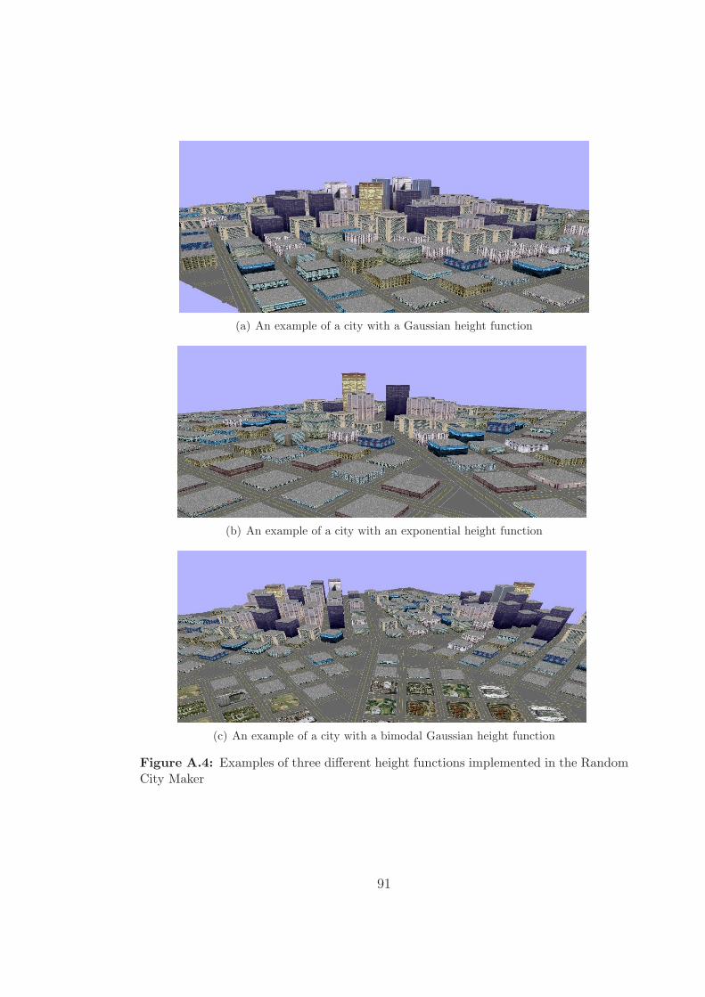
(a) An example of a city with a Gaussian height function
(b) An example of a city with an exponential height function
(c) An example of a city with a bimodal Gaussian height function
Figure A.4: Examples of three different height functions implemented in the RandomCity Maker
91
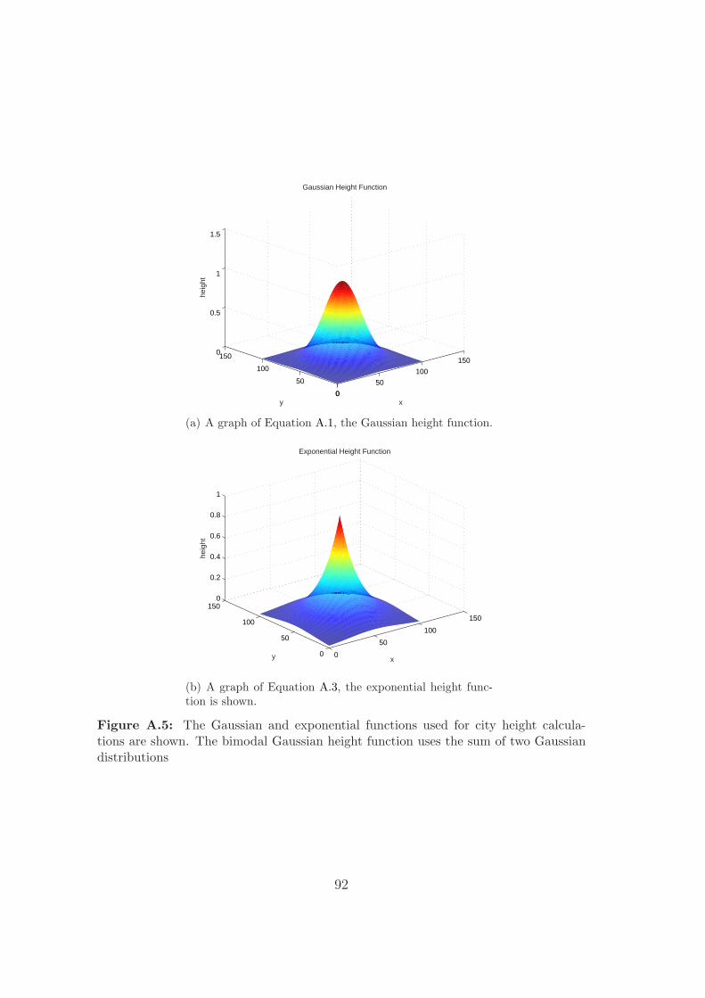
0
50
100
150
0
50
100
1500
0.5
1
1.5
x
Gaussian Height Function
y
heig
ht
(a) A graph of Equation A.1, the Gaussian height function.
0
50
100
150
0
50
100
1500
0.2
0.4
0.6
0.8
1
x
Exponential Height Function
y
heig
ht
(b) A graph of Equation A.3, the exponential height func-tion is shown.
Figure A.5: The Gaussian and exponential functions used for city height calcula-tions are shown. The bimodal Gaussian height function uses the sum of two Gaussiandistributions
92