political decentralization and corruption: evidence from around the world

Journal of Public Economics 93 (2009) 14–34

Contents lists available at ScienceDirect

Journal of Public Economics

j ourna l homepage: www.e lsev ie r.com/ locate /econbase

Political decentralization and corruption: Evidence from around the world☆

C. Simon Fan a, Chen Lin b, Daniel Treisman c,⁎a Department of Economics, Lingnan University, Hong Kongb Department of Economics and Finance, City University of Hong Kong, Hong Kongc Department of Political Science, University of California, Los Angeles, 4289 Bunche Hall, Los Angeles, CA 90095-1472, United States

a r t i c l e i n f o

☆ We thank Robin Boadway (the editor) and two anothe paper a lot.⁎ Corresponding author. Tel.: +1 310 968 3274; fax:

E-mail address: [email protected] (D. Treis

0047-2727/$ – see front matter © 2008 Elsevier B.V.doi:10.1016/j.jpubeco.2008.09.001

a b s t r a c t

Article history:Received 11 September 2007Received in revised form 9 September 2008Accepted 10 September 2008Available online 16 September 2008

How does political decentralization affect the frequency and costliness of bribe extraction bycorrupt officials? Previous empirical studies, using subjective indexes of perceived corruption andmostly fiscal indicators of decentralization, have suggested conflicting conclusions. In search ofmore precise findings, we combine and explore two new data sources—an original cross-nationaldata set on particular types of decentralization and the results of a firm level survey conducted in80 countries about firms' concrete experiences with bribery. In countries with a larger number ofgovernment or administrative tiers and (given local revenues) a larger number of local publicemployees, reported bribery wasmore frequent.When local—or central—governments received alarger share of GDP in revenue, briberywas less frequent. Overall, the results suggest the danger ofuncoordinated rent-seeking as government structures become more complex.

© 2008 Elsevier B.V. All rights reserved.

Keywords:CorruptionDecentralizationPolitical economy

1. Introduction

How does political decentralization affect the frequency and the costliness of corrupt bribe extraction by officials? Theoriessuggest conflicting conclusions. On one hand, by bringing officials “closer to the people” or encouraging competition amonggovernments for mobile resources, decentralization might increase government accountability and discipline. On the other hand,decentralization could impede coordination and exacerbate incentives for officials at different levels to “overgraze” the commonbribe base. More generally, one might expect a variety of effects associated with different types of decentralization to operatesimultaneously, pulling in many directions, with different strength in different contexts.

A number of scholars have sought to answer this question empirically by looking for relationships between measures ofpolitical or fiscal decentralization and cross-national indexes of perceived corruption derived from surveys of risk analysts,businessmen and citizens. In particular, scholars have examined perceived corruption ratings produced by TransparencyInternational (TI), the World Bank (WB), and the business consultancy Political Risk Services, which publishes the InternationalCountry Risk Guide (ICRG). The findings of these studies have been mixed and sometimes mutually contradictory.

Focusing on fiscal decentralization, Huther and Shah (1998), De Mello and Barenstein (2001), Fisman and Gatti (2002), and Arikan(2004) all report that a larger subnational share of public expenditures (as measured in the IMF's Government Finance Statistics) wasassociated with lower perceived corruption using the TI, ICRG, or WB indexes. Enikolopov and Zhuravskaya (2007) do not report anunconditional effect, but find that a larger subnational revenue share is associatedwith lower perceived corruption (usingWB, but not TI,data) in developing countries with older political parties (and vice versa); a larger subnational revenue share in developing countrieswhere there are fewparties in government is associatedwith lower corruption (on bothWB and TImeasures) (and vice versa). Looking atpolitical rather than fiscal indicators, Goldsmith (1999), Treisman (2000), and Kunicová and Rose-Ackerman (2005) all found that federal

nymous referees for many constructive comments and suggestions that have helped improve the quality o

+1 310 825 0778.man).

All rights reserved.

f

mailto:[email protected]

http://dx.doi.org/10.1016/j.jpubeco.2008.09.001

http://www.sciencedirect.com/science/journal/00472727

15C.S. Fan et al. / Journal of Public Economics 93 (2009) 14–34

structurewas associatedwith higher perceived corruption. However, in amore recent reviewof the empirical literature, Treisman (2007)suggested that neither the (negative) expenditure decentralization effect nor the (positive) federalism effect was robust. The fiscaldecentralization effect was weakened by controlling for national religious traditions, and the federal effect disappeared as the number ofcountries in the sample increased. Treisman (2002) and Arikan (2004) explored whether smaller local units were associated with lesscorruption because of more intense interjurisdictional competition, but obtained inconclusive results. Finally, examining the effect of thevertical structure of states, Treisman (2002) found that a larger number of administrative or governmental tiers correlated with higherperceived corruption, but whether subnational governments were appointed or elected did not have a clear effect.

In this paper, we advance and improve upon this literature in three ways. First, our analysis exploits an original cross-nationaldata set on different varieties of decentralization, compiled from more than 480 sources. This allows us to design indicators ofparticular types of decentralization to match the underlying logic of specific arguments. We look for relationships betweenreported experience with corruption and: (i) the number of tiers of government or administration in the country (see Section 3.1),(ii) the average land area of lowest tier units (see Section 3.2), (iii) several proxies for the extent of subnational politicaldecisionmaking (see Section 3.2 and others), (iv) an indicator for whether lower tier units have elected executives (see Section 3.3),(v) a measure of subnational tax revenues as a share of GDP (see Section 3.4), and (vi) an estimate of the share of subnationalgovernment personnel in total civilian government personnel (see Section 3.5).

Second, most previous studies have used perceived corruption indexes that rely on the aggregated perceptions of businessmen orcountry experts, many of whom may have formed impressions—perhaps subconsciously—based on common press depictions ofcountries or conventional notions aboutwhat institutions or cultures are conducive to corruption.More recently, a second type of datahas become available: survey responses of businessmen and citizens in particular countries about their own (or close associates')concrete experiences with corrupt officials. In a recent study, Treisman (2007) showed that, for developing countries, the perceivedcorruption indexes were relatively weakly correlated with experience-based indicators. Among countries rated as highly corrupt onthe subjective indexes of TI,WB, and the ICRG, there is great variation in the level of reported experiencewith corruption. For instance,on the World Bank perceived corruption index, Argentina and Macedonia were both rated about equally corrupt in 2000: they wereranked 103 and 114 respectively out of 185 countries. But respondents from these two countries gave dramatically different answerswhen surveyed by the United Nations Interregional Crime and Justice Research Institute (UNICRI) in the late 1990s about their ownpersonal experience with bribery. When asked whether during the previous year “any government official, for instance a customsofficer, policeofficer or inspector”had askedor expected them topaya bribe forhis services, respondents inArgentinawere three and ahalf times as likely as theMacedonian respondents to say yes.While Argentina had the secondhighest frequency of reported demandsfor bribes (second only to Indonesia), Macedoniawas only 24th in the list of 49 countries, about evenwith South Africa and the CzechRepublic. Perhaps of greater concern, a number of factors commonly believed to affect corruption (democracy, press freedom, oil rents,even the percentage of women in government) do an excellent job explaining the cross-national variation in the subjective corruptionindexes (R-squareds approaching .90). But the same factors are mostly uncorrelated with the frequency or scale of self-reportedexperiences with corruption once one controls for income. One cannot help wondering if the businessmen and experts whoseperceptions are being tapped might be inferring corruption levels from its hypothesized causes.

In this study, we explore the results of an experience-based survey of business managers conducted in 80 countries. The WorldBusiness Environment Survey interviewed managers from more than 9000 firms in 1999–2000. We focus on two questions.Respondents were asked: “Is it common for firms in your line of business to have to pay some irregular ‘additional payments’ to getthings done?” and “On average, what percent of total annual sales do firms like yours typically pay in unofficial payments/gifts topublic officials?” The first question provides an indicator of the frequency of bribery, while the second aims to estimate its scale.The relationship between the proportion of respondents that said irregular payments were expected “always”, “mostly”, or“frequently”, and theWorld Bank's subjective index of perceived corruption for the year 2000 are graphed in Fig. 1. It is interestingto note that while businessmen in France and Brazil gave very similar responses to this question (about 27% saying bribes wereexpected “always”, “mostly”, or “frequently”), France is rated as among the least corrupt countries on theWorld Bank's index, whileBrazil is perceived to have much higher corruption. Of course, no approach is completely without problems; it is possible thatquestions that focus more closely onmanagers' direct experience with corruptionmight not be answered with complete franknessfor fear of some kind of self-incrimination. However, we believe this danger is less serious than the danger that bias will creep intothe assessments of “experts” and foreign businessmen because of inconsistencies in media coverage. (As a robustness check, wecompare our results to those obtained using the traditional perceived corruption data.)

Third, besides permitting us to focus on experience-based rather than subjective indicators of corruption, the WBES makes itpossible to control better for individual characteristics of survey respondents (which vary systematically across countries).Specifically, we can control for the size, ownership structure, investment level, and level of exports of firms in analyzing theirmanagers' responses on corruption.

In the next section, we briefly introduce the decentralization data used in the paper. We review common arguments about theconsequences of decentralization for governance in Section 3, and in Section 4 discuss the corruption data and controls. We thenlook for evidence of the hypothesized effects in the WBES. In Section 5 we present empirical results and discuss robustness tests.Section 6 discusses the findings and concludes.

2. A new data set on governance in multi-level states

Previous work has often used measures of fiscal decentralization or simple dummies for federal structure to proxy for variousother types or dimensions of political and administrative decentralization. The data set introduced here permits a more fine-

Fig. 1. Subjective and experience-based indicators of corruption, 2000.

16 C.S. Fan et al. / Journal of Public Economics 93 (2009) 14–34

grained analysis. It contains measures of various characteristics of multi-level states as of the mid-1990s, based on informationfrom more than 480 sources.1

A first dimension is simply the number of tiers of government or administration. Our data set contains information on this for 156countries.We coded a level of administration as a “tier” if there existed a state executive bodyat that levelwhichmet three conditions:(1) it was funded from the public budget, (2) it had authority to administer a range of public services, and (3) it had a territorialjurisdiction. This definition includes both bodies with decisionmaking autonomy and those that are essentially administrative agentsof higher level governments. On this measure, Singapore as of the mid-1990s had just one tier, while Uganda had six.

Multi-level states differ also in the number and size of their lowest tier units. This is relevant, for instance, to arguments aboutinterjurisdictional mobility. The data set contains estimates of the number of bottom level units (Bottom units), and the “average”area of these (Bottom size), calculated by simply dividing the country's area by the number of units.2 While Guyana in the mid-1990s had just six incorporated towns, India had some 235,000 lower tier village governments. The average area of the lowest tierunits ranged from 2.2km2 in Bangladesh to 83km2 in Botswana.

Perhaps most important, multi-level governments differ in how authority is divided among the various tiers. Measuring thedegree of decisionmaking autonomy of local governments in a systematic way is notoriously difficult. Our data set contains asimple dummy (Autonomy), which records for 133 countries whether the constitution assigned at least one policy area exclusivelyto subnational governments or gave subnational governments exclusive authority to legislate on matters not constitutionallyassigned to any level. This variable is less than ideal. For one thing, informal behavior often diverges from what is written in theconstitution. In some countries—Azerbaijan and Uzbekistan, for instance—it seems unlikely the constitutional provisions arescrupulously observed.3 Yet determining the degree of actual decisionmaking decentralization in any country is inescapablysubjective. Experts often disagree with regard to a single country, let alone agreeing on cross-national comparisons. At the sametime, the number and relative importance of policy areas constitutionally assigned to subnational governments differs, and there isno obvious way to add these up. Autonomy also focuses mostly on intermediate levels—states, provinces, or regions—whereas thegovernments most relevant to questions of interregional competition will often be at the local level. We supplement the use of

1 These data and the full list of sources will be made available on the corresponding author's web site.2 A better variable would be the average area of all actual units, but data were not available. Since the number of bottom-tier units changes over time as units

split or combine, the variable is only a rough indicator.3 Both inherited Soviet-era internal “autonomous republics”, whose rights are constitutionally protected.

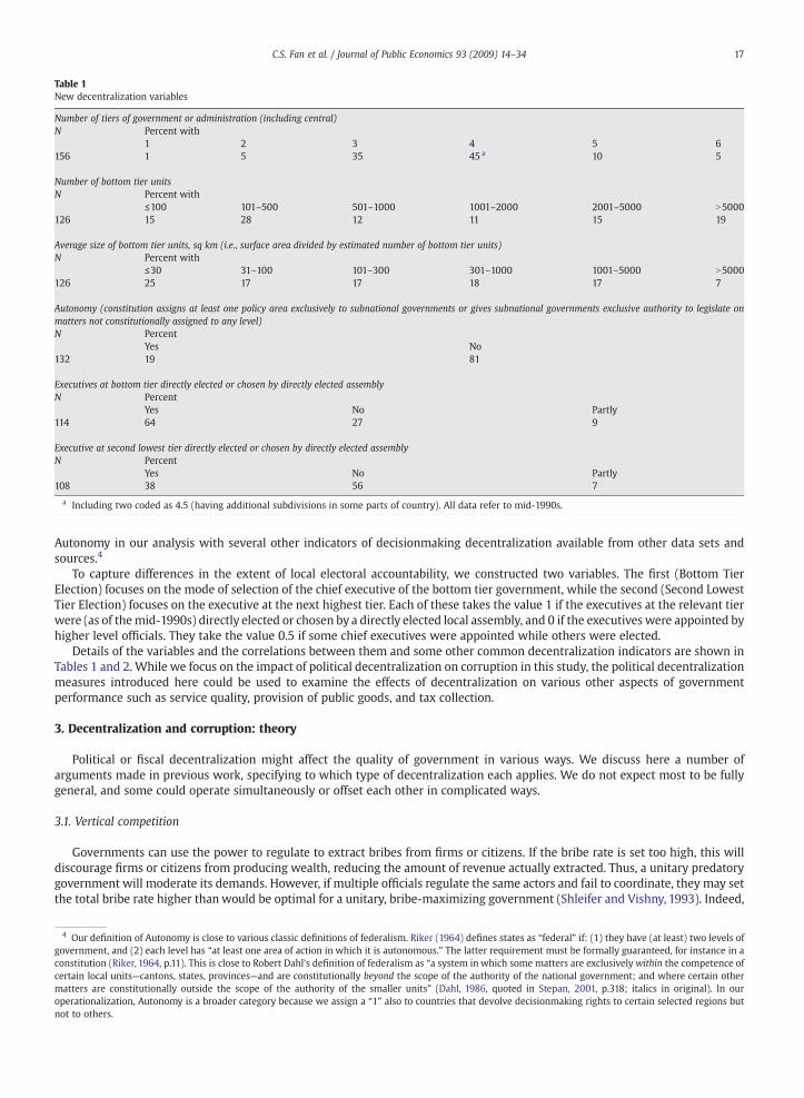
Table 1New decentralization variables

Number of tiers of government or administration (including central)N Percent with

1 2 3 4 5 6156 1 5 35 45 a 10 5

Number of bottom tier unitsN Percent with

≤100 101–500 501–1000 1001–2000 2001–5000 N5000126 15 28 12 11 15 19

Average size of bottom tier units, sq km (i.e., surface area divided by estimated number of bottom tier units)N Percent with

≤30 31–100 101–300 301–1000 1001–5000 N5000126 25 17 17 18 17 7

Autonomy (constitution assigns at least one policy area exclusively to subnational governments or gives subnational governments exclusive authority to legislate onmatters not constitutionally assigned to any level)N Percent

Yes No132 19 81

Executives at bottom tier directly elected or chosen by directly elected assemblyN Percent

Yes No Partly114 64 27 9

Executive at second lowest tier directly elected or chosen by directly elected assemblyN Percent

Yes No Partly108 38 56 7

a Including two coded as 4.5 (having additional subdivisions in some parts of country). All data refer to mid-1990s.


Autonomy in our analysis with several other indicators of decisionmaking decentralization available from other data sets andsources.4

To capture differences in the extent of local electoral accountability, we constructed two variables. The first (Bottom TierElection) focuses on the mode of selection of the chief executive of the bottom tier government, while the second (Second LowestTier Election) focuses on the executive at the next highest tier. Each of these takes the value 1 if the executives at the relevant tierwere (as of themid-1990s) directly elected or chosen by a directly elected local assembly, and 0 if the executives were appointed byhigher level officials. They take the value 0.5 if some chief executives were appointed while others were elected.

Details of the variables and the correlations between them and some other common decentralization indicators are shown inTables 1 and 2. While we focus on the impact of political decentralization on corruption in this study, the political decentralizationmeasures introduced here could be used to examine the effects of decentralization on various other aspects of governmentperformance such as service quality, provision of public goods, and tax collection.

3. Decentralization and corruption: theory

Political or fiscal decentralization might affect the quality of government in various ways. We discuss here a number ofarguments made in previous work, specifying to which type of decentralization each applies. We do not expect most to be fullygeneral, and some could operate simultaneously or offset each other in complicated ways.

3.1. Vertical competition

Governments can use the power to regulate to extract bribes from firms or citizens. If the bribe rate is set too high, this willdiscourage firms or citizens from producing wealth, reducing the amount of revenue actually extracted. Thus, a unitary predatorygovernment will moderate its demands. However, if multiple officials regulate the same actors and fail to coordinate, they may setthe total bribe rate higher thanwould be optimal for a unitary, bribe-maximizing government (Shleifer and Vishny, 1993). Indeed,

4 Our definition of Autonomy is close to various classic definitions of federalism. Riker (1964) defines states as “federal” if: (1) they have (at least) two levels ofgovernment, and (2) each level has “at least one area of action in which it is autonomous.” The latter requirement must be formally guaranteed, for instance in aconstitution (Riker, 1964, p.11). This is close to Robert Dahl’s definition of federalism as “a system in which some matters are exclusivelywithin the competence ofcertain local units—cantons, states, provinces—and are constitutionally beyond the scope of the authority of the national government; and where certain othermatters are constitutionally outside the scope of the authority of the smaller units” (Dahl, 1986, quoted in Stepan, 2001, p.318; italics in original). In ouroperationalization, Autonomy is a broader category because we assign a “1” also to countries that devolve decisionmaking rights to certain selected regions butnot to others.

Table 2Correlations between decentralization variables (and ln GDP per capita)

Numberof tiers

Bottomunits

Bottomsize

Autonomy BottomTierElection

SecondLowest TierElection

Federal(Elazar,1995)

Subnationalrevenues(% GDP)

Subnationalexpenditures(% total govexpenditures)

Subnational %of total civiliangov employment

Number of tiers 1Bottom units .371 1Bottom size − .118 − .073 1Autonomy .044 .157 − .060 1Bottom Tier Election − .131 .144 − .020 .010 1Second Lowest Tier Election − .069 .069 − .064 .157 .433 1Federal (Elazar, 1995) .017 .218 − .037 .738 .102 .243 1Subnational revenues (% GDP) − .029 − .002 − .116 .418 .120 .197 .445 1Subnational expenditures

(% total gov expenditures).114 .211 − .152 .486 .203 .271 .585 .815 1

Subnational% % of total civiliangov employment

.031 .085 − .124 .328 .460 .231 .375 .516 .718 1

Ln GDP per capita 1999 − .485 − .100 − .053 .249 .337 .227 .264 .306 .210 .298


the aggregate bribe burden is likely to increase with the number of independent regulators. If officials at each tier in a multi-levelstate can regulate, the burden of bribery should increase with the number of tiers. The logic is that of “double marginalization”under vertical integration (Spengler, 1950) or “overgrazing” in taxation (Keen and Kotsogiannis, 2002; Berkowitz and Li, 2000).5

Although appealing, this argument might fail for various reasons. The number of independent regulators might not increasewith the number of tiers. In fact, administrative complexity at the center and decentralization might be substitutes—to governdirectly, a central government may need to create more agencies in the capital to take the place of local field agents. Moreover,career concerns might motivate local officials in a decentralized state to behave honestly. The hope of rising to higher office maycause local officials to cultivate a reputation for integrity (Myerson, 2006). Finally, if elected governments at different levels providecomparable public goods, some scholars suggest theymay be disciplined by yardstick competition. Voters can use the performanceof each as a benchmark to judge the efficiency of the other (Salmon,1987; Breton,1996, p.189). If one government over-regulates inorder to extract bribes, its performance will look bad in comparison to its more liberal counterparts at other levels. To test thisargument, we use the variable Tiers, measuring the number of levels of government or administration.

3.2. Interregional competition

If capital or labor is mobile and local governments choose policies, they may tailor these to attract the mobile factor (Hayek,1939; Tiebout, 1956). Officials who steal or waste resources will lose residents and businesses to other regions, reducing their taxbase. If they over-regulate in order to extract bribes, firms will flee to lower-regulation settings. In this way, interjurisdictionalcompetition may discipline local governments, reducing corruption and causing them to supply public goods efficiently (Brennanand Buchanan, 1980; Montinola et al., 1995). The impact of such competition should be greater, the lower the cost of movingbetween units; moving costs should increase with the size of the units.

However, the fear of losingmobile capitalmay fail to discipline local governments for a numberof reasons (e.g., Cai and Treisman,2005). Or governmentsmaycompete to attract capital bypromising corrupt benefits to local businesses at the expense of the centralgovernment (Cai and Treisman, 2004). Even if interjurisdictional competition motivates local politicians to reduce corruption, itdoes not increase their capacity to do so. If most bribes are taken by local bureaucrats and anti-corruption measures must beimplemented by the same bureaucrats, it may matter little how motivated the politicians are to clean up government. And if anti-corruption measures are costly, the inability to tax mobile capital may make it harder for local governments to fund such efforts.

The relevant type of decentralization here is devolution of decisionmaking about regulation or taxation to subnational levels;among countries with a similar level of such devolution, one might expect a positive correlation between average size of thesubnational units and corruption. To measure devolution of decisionmaking, we start with the variable Autonomy. But wesupplement it with various alternatives. First, we created a dummy for whether the country was classified as “federal” by a leadingexpert on federalism as of the mid-1990s (Federal) (Elazar, 1995). Second, in an attempt at a more fine-grained analysis, we triedusingmeasures of the extent of decisionmaking decentralization in specific public service areas, constructed by Henderson (2000).Henderson coded whether, in 49 countries in 1960–95, authority for primary education, local highway construction, and localpolicing belonged to the central, regional, or local governments, or some combination of the three.6 (Of these 49 countries, 35wereincluded in theWBES.) Both local road construction and local policing could impinge on the operations of almost any business, but itis harder to see how the regulation of primary schooling could lend itself towidespread extraction of bribes from businesses, so we

5 In a notable recent contribution,Olken and Barron (2007) find evidence consistent with double-marginalization using Indonesian data.6 The details of the data set constructed by Henderson (2000) can be obtained through direct communications with Henderson.


focused on the former two indicators. We constructed two variables (Roads local and Police local) which took the value 1 if, as of1995, the local governments participated in decisionmaking on the issue in question, and 0 otherwise.7 The arguments in Section 3.2suggest that when Roads local and/or Police local equal one, greater factor mobility might be associated with lower corruption. Tocapture the average size of subnational units, which should be positively related to moving costs, we used our variable Bottom size.

3.3. Electoral accountability

For several reasons, holding elections at the local level rather than just the center might increase the accountability ofgovernment (see e.g. Seabright, 1996). First, voters might have better information about local than about central governmentperformance. Second, whereas national elections focus on government performance nationwide, local elections can focus morespecifically on performance in each region. Third, dividing up responsibilities among several levels of elected government mightmake it easier for voters to attribute credit or blame among them (under decentralization, one can vote for an honest centralgovernment and against a corrupt local government rather than having to vote for or against the team as a whole).8 Fourth, thesmaller a unit's electorate, the easier it should be for voters to coordinate on a voting strategy to discipline the incumbent.

Questions can be raised about each of these arguments. First, local corruption can be concealed at least as well as centralcorruption, and watchdog groups and investigative journalists tend to devote more resources to monitoring national governmentsince the stakes are generally higher. Second, voters evaluate incumbents on multiple dimensions and it is not clear whethercorruptionwill be more salient in local or in national elections. Even if voters voted on just the corruption question, competition ina national election should often motivate central candidates to fight corruption in each district (if they do not, their adversary will,winning votes in the affected unit). Third, dividing responsibilities among levels may muddle rather than clarify the attribution ofresponsibility (compare a system inwhich two levels share responsibility for all policy areas to one inwhich a central governmentis alone responsible for all). Finally, coordinating is only significantly easier in groups that are very small (and smaller than theelectorates of most existing local districts). Even in tiny villages, there are many dimensions on which voters could judge localofficials, rendering coordination to discipline them on corruption problematic.9 To capture differences in the extent of localelectoral accountability, we used the variables Bottom Tier Election and Second Lowest Tier Election.

3.4. Fiscal incentives

Thegreater is corruption, the lowerwill be themotivationoffirms toproduce.Given this, someargue that corruptionwill fall if localofficials are given a large personal stake in local economic activity. Under tax-sharing systems, the larger the share local governmentsretain of marginal tax revenues, the lower should be their incentive to extract bribes (Montinola et al., 1995; Zhuravskaya, 2000; Jinet al., 2005). Since the argument relates to themarginal rate atwhich local governments benefit from increased local business activity,the relevant variable is the local governments' revenue as a share of local income at themargin. As usual, there are caveats. Increasinglocal governments' share means decreasing the shares of other levels. If local governments become more motivated to supporteconomic performance, governments atother levels should become lessmotivated. Since, for better orworse, governments at all levelsinfluence economic performance, the resulting net effect is indeterminate (Treisman, 2006). Moreover, local officials may derivegreater utility from bribe revenue, which they can spend at will, than from increased revenue officially received by the local budget,whichmaybe costly to embezzle. If officials are already constrained by the risk of detection fromembezzlingmore, then increasing thelocal tax share may not make themwant to reduce their bribe taking in order to expand the local budget.

To test this argument, we use subnational government revenues as a percentage of GDP. The data are mostly from the IMF'sGovernment Finance Statistics Yearbooks (as collected in theWorld Bank's database of fiscal decentralization indicators), supplementedby additional sources on specific countries. We took the average value for all available years between 1994 and 2000. There are somemissingobservations in this variable so the sample size falls from67 countries (6676 observations) to 54 countries (5598observations)when we include it. Some previous studies used a variable measuring the share of local revenues or expenditures in total publicrevenues or expenditures to look for the effects offiscal decentralization.However, since the argument here concerns the share of localincome that local governments retain through taxation, we prefer an indicator that measures this more closely—the share of localrevenues in GDP.

A better variable would have been the marginal revenue rate for local governments from locally generated income; however,cross-national data onmarginal rates were not available, so we had to use the average rate instead. We control in these regressionsfor total government revenues as a share of GDP, since larger government might be associated with both greater corruption andhigher local taxation.

7 In only one case—local highway construction in Uganda—did the local governments enjoy exclusive authority. We also constructed an indicator (SharedResponsibility) for the number of government levels participating in decisionmaking in these two policy areas (the more governments involved, the greater thepotential for predatory extraction and “overgrazing”). Values ranged from 2 if for both local highways and policing only one level could make policy (as in Syria orEgypt), to 6 if, for both areas, all three levels of government could participate (as in the US). From the arguments in Section 3.1, one might expect SharedResponsibility to correlate positively with corruption. In fact, it was never significant, so we do not show results including it.

8 Besley and Coate (2003) make a similar argument about why direct election of regulators—rather than their appointment by elected officials—might lead togreater responsiveness to voters by reducing the number of issues on which each vote is cast.

9 Electoral decentralization also eliminates accountability of local officials to voters outside their unit, which might itself increase some kinds of corruption. Alocally elected sheriff could increase his town's revenues, taking a cut for himself, by inaccurately citing out-of-town motorists for speeding.


3.5. Local collusion

Some economists suggest local officials are simply more susceptible to corruption than their central counterparts, perhapsbecause they have more opportunities for face-to-face interactions with businessmen (e.g., Prud'homme, 1995; Tanzi, 1996;Bardhan and Mookherjee, 2000) Local press and citizen groups may be weaker—and more subject to intimidation or cooptation—than at the center. Interest groups may be more cohesive at the local level, leading to greater state capture. By this logic,government should be more corrupt, the greater the share of government personnel located at subnational levels.

However, one could also argue the opposite. Even if the intimacy of interaction and the cohesiveness of interest groups aregreater at the local level, the potential kickbacks and payoffs in national politics are likely to be higher. As noted in Section 3.3,voters are often assumed to be better informed about their local governments than about politics in the nation's capital. In any case,the real question is not whether local governments are likely to be more corrupt than central governments but whether electedlocal governments with decisionmaking power are likely to be more or less corrupt than centrally appointed local agents withmore restricted authority. Whether there is a general answer to this question is unclear. To test this argument, we constructed ameasure of government personnel decentralization—the subnational share in total civilian government employees as of the mid-1990s, as estimated by Schiavo-Campo et al. (1997). We control for total government employment as a share of the labor force,since, as noted, the size of government as a whole might itself be related to corruption.

4. Corruption data and controls

4.1. The survey

The WBES was conducted in 1999 and 2000 by a team from the World Bank. Managers from over 9000 firms in more than 80countries were surveyed with a standard questionnaire.10 The main purpose was to identify the driving factors behind andobstacles to enterprises' performance and growth around the world. The questionnaire touched on many aspects of firms'operations, including corruption, regulation, and the institutional environment. The firms surveyed varied in size (including a largenumber of small and medium-size enterprises), ownership (both public and private), industrial sector, and organizationalstructure. Because of missing firm level and decentralization variables, the number of firms we could include in our analysis startsat about 6700 (from 67 countries), and falls lower as additional variables are added. Previouswork has used theWBES data to studysuch outcomes as firm growth, investment flows, the effects of institutions, property rights, and corruption (Hellman et al., 2000;Djankov et al., 2003; Beck et al., 2005; Acemoglu and Johnson, 2005; Beck et al., 2006; Ayyagari et al., in press; Barth et al., in press).According to Reinikka and Svensson (2006, p.367), the WBES shows that “with appropriate survey methods and interviewtechniques, it is possible to collect quantitative data on corruption at the micro-level.”

4.2. Measures of corruption

We constructed twomeasures of corruption usingWBES data. The first, whichwe call Bribe Frequency, is based on a question inwhich respondents were asked: “Is it common for firms in your line of business to have to pay some irregular ‘additional payments’to get things done.” The interviewers assured respondents that their responses would be kept completely confidential, and thattheir names and the names of their firms would never be identified in any publication or survey document. In addition, toencourage honest responses, the question asked only about unofficial payments “in your line of business” rather than those “paidby your firm” (Johnson et al., 2002). Managers could choose between six responses: 1 (never), 2 (seldom), 3 (sometimes), 4(frequently), 5 (usually), and 6 (always). Thus, the variable Bribe Frequency takes these six values; a larger value represents morefrequent bribery payments.11 Overall, about 69% of respondents (6300 out of 9130) reported that firms like theirs paid bribes topublic officials to get things done. About 15% of the firms reported that this occurred “4 ( frequently),” 12% reported “5 (usually),”and 9% reported “6 (always)”. In countries such as Bangladesh, Nigeria, Tanzania, Thailand, Uganda, and Zimbabwe, more than 90%of the firms sampled reported that such unofficial payments occurred at least occasionally. The lowest rate of reported bribery wasin Singapore, where 90% said firms like theirs never had to make unofficial payments.

Our second measure, which we call Bribe Amount, was constructed from a question that asked: “On average, what percent oftotal annual sales do firms like yours typically pay in unofficial payments/gifts to public officials?” The survey offered sevenchoices: (1) 0%, (2) 0–1%, (3) 1–1.99%, (4) 2–9.99%, (5) 10–12%, (6) 13–25%, and (7) over 25 percent. Out of the original sample of 80countries, respondents in 60 countries answered this question. Overall, more than 62% of thosewho responded reported that firmslike theirs typically made positive unofficial payments to public officials. More than 38% reported that such payments were greaterthan 1% of total sales; about 11% said payments exceeded 10% of total sales. The average size of such payments varied across bothcountries and the firms within them.

The twomeasures of corruption are complementary, capturing different dimensions that may not always coincide (bribes couldbe frequent but tiny, or rare but large). In some respects, the amount of bribes paid is themore interesting variable. However, it wasalso apparently perceived by respondents as more sensitive: in one quarter of the countries, respondents did not answer this

10 For more information on the survey, see http://www.ifc.org/ifcext/economics.nsf/Content/ic-wbes.11 The original survey offered the six choices in reverse order: (1) always, (2) mostly, (3) frequently, (4) sometimes, (5) seldom, (6) never. We recoded thevariable to make the empirical results more intuitive.

http://www.ifc.org/ifcext/economics.nsf/Content/ic-wbes

Table 3Description and sources of key variables

Variable Description Source WBES countries missing from data

Firm characteristics and corruption measuresBribe Frequency It is common for firms in my line of business to have to pay

some irregular “additional payments” to get things done:(1) never, (2) seldom, (3) sometimes. (4) frequently, (5) mostly,(6) always.

World Business Environment Survey (WBES)

Bribe Amount On average, what percentage of revenues do firms like yourstypically pay per year in unofficial payments to public officials:(1) 0%, (2) greater than 0 and less than 1%, (3) 1–1.99%,(4) 2–9.99%, (5) 10–12%, (6) 13–25%, (7) over 25%.


Foreign Ownership Dummy variable that equals 1 if any foreign company orindividual has a financial stake in the ownership of thefirm, 0 otherwise


State Ownership Dummy variable that equals 1 if any government agency orstate body has a financial stake in the ownership of thefirm, 0 otherwise


Exporter Dummy variable that equals 1 if firm exports, 0 otherwise. World Business Environment Survey (WBES)Firm Size Natural logarithm of firm's sales World Business Environment Survey (WBES)Industry Dummies A series of dummy variables that represent the firms'

industries (Manufacturing, Construction, Service,Agriculture, and Others)


Political and fiscal decentralization measuresTiers Number of tiers of government. A tier is coded as a “tier

of government” if state executive body at that level480 sources, detailed in Fan et al. (2008) Belize, Cote d'lvoire, West Bank-Gaza

(1) was funded from the public budget, (2) had authorityto administer a range of public services, and (3) had aterritorial jurisdiction.

Federalism Dummy variable that takes the value 1 if the country isclassified as “federal”, 0 otherwise.

Elazar (1995) Belize, Cote d'lvoire, West Bank-Gaza

Bottom unit size Average size of bottom tier units, thousand sq km(i.e., surface area divided by estimated number of bottomtier units)

480 sources, detailed in Fan et al. (2008) Belize, Cameroon, China, Cote d'lvoire, Kenya, Nigeria,Senegal, Singapore, Tanzania, West Bank-Gaza

Autonomy Dummy variable that takes the value 1 if (1) constitutionreserves decisionmaking on at least one topic exclusivelyto subnational legislatures and/or (2) constitution assignsto subnational legislatures exclusive right to legislate onissues that it does not specifically assign to one level ofgovernment.

Constitutions of countries in data set Belize, Botswana, Cameroon, Dominican Rep, Ecuador,El Salvador, Guatemala, Honduras, Nicaragua, Nigeria,Panama, Tanzania, Ukraine, Uruguay, West Bank-Gaza

(continued on next page)(continued on next page)

21C.S.Fan

etal./

Journalof

PublicEconom

ics93

(2009)14

–34

Table 3 (continued)

Variable Description Source WBES countries missing from data

Bottom Tier Election Variable that takes the value: 1 if executives at bottom tierare directly elected or chosen by directly elected assembly;0 if executives at bottom tier are appointed by the officials inhigher tier government unit; 0.5 if some of the executives areappointed while some of them are elected.

480 sources, detailed in Fan et al. (2008) Armenia, Azerbaijan, Bangladesh, Belize, Botswana,Cambodia, Cameroon, China, Cote d'lvoire, Ethiopia,Ghana, Guatemala, India, Madagascar, Malawi, Moldova,Pakistan, Singapore, West Bank-Gaza

Second Lowest TierElection

Variable that takes the value: 1 if executives at second lowesttier are directly elected or chosen by directly elected assembly;0 if executives at second lowest tier are appointed by theofficials in higher tier government unit; 0.5 if some of theexecutives are appointed while some of them are elected.

480 sources, detailed in Fan et al. (2008) Armenia, Azerbaijan, Belize, Cambodia, Cameroon, China,Cote d'lvoire, Ethiopia, Ghana, Guatemala, India, Madagascar,Malawi, Moldova, Nicaragua, Pakistan, Singapore, Slovenia,Thailand, Trinidad Tobago, Uruguay, West Bank-Gaza,Zimbabwe

Subnational revenues Subnational revenues (% of GDP), average 1994–2000,available years, from World Bank DecentralizationIndicators, constructed from IMF GFS

World Bank Decentralization Indicators (2007) Bangladesh, Belize, Bosnia, Cambodia, Cameroon, Cote d'lvoire,Ecuador, Egypt, Ethiopia, Guatemala, Haiti, Honduras,Madagascar, Malawi, Namibia, Pakistan, Tanzania, Tunisia,Turkey, Venezuela, West Bank-Gaza

Subnational governmentemployment share:

Non-central government employment as % of totalgovernment employment.

Schiavo-Campo et al. (1997) Azerbaijan, Bangladesh, Belize, Bosnia, Brazil, Cambodia,Costa Rica, Cote d'lvoire, Czech Rep., Dominican Rep.,El Salvador, Ethiopia, Guatemala, Haiti, Kyrgyzstan,Madagascar, Malawi, Malaysia, Mexico, Namibia, Nicaragua,Nigeria, Panama, Peru, Romania, Slovenia, Trinidad Tobago,Uzbekistan, West Bank-Gaza

Total governmentrevenues

Total government revenues (% of GDP), average 1994–2000,available years, from World Bank DecentralizationIndicators, constructed from IMF GFS

World Bank Decentralization Indicators (2000) Bangladesh, Belize, Bosnia, Botswana, Cambodia, Cameroon,Colombia, Cote d'lvoire, Ecuador, Egypt, El Salvador, Ethiopia,Guatemala, Haiti, Honduras, Madagascar, Malawi, Namibia,Nigeria, Pakistan, Philippines, Senegal, Singapore, Tanzania,Tunisia, Turkey, Uruguay, Venezuela, West Bank-Gaza

Total governmentemployment

Total government employment as a share of labor force. Schiavo-Campo et al. (1997) Azerbaijan, Bangladesh, Belize, Bosnia, Brazil, Cambodia,Costa Rica, Cote d'lvoire, Czech Rep., Dominican Rep.,El Salvador, Ethiopia, Guatemala, Haiti, Kyrgyzstan,Madagascar, Malawi, Mexico, Namibia, Nicaragua, Nigeria,Panama, Peru, Romania, Slovenia, Trinidad Tobago, Uzbekistan,West Bank-Gaza

Other macro control variablesGDP per Capita Natural logarithm of country's GDP per capita in year 1999 WDI 2006 (World Bank)Democratic Democratic in all years 1950–2000 Treisman (2000), Przeworksi et al. (2000) Belize, Cote d'lvoire, West Bank-GazaFuel % of mineral fuels in manufacturing exports, 2000 WDI 2006 (World Bank) Belize, Bosnia, Cote d'lvoire, Dominican Rep, Ethiopia, Haiti,

Kyrgyzstan, Uzbekistan, West Bank-GazaImports Imports of goods and services as % of GDP, 2000 WDI 2007 (World Bank) Belize, Cote d'lvoire, Singapore, West Bank-GazaProtestant Protestant as % of the population Barro and McCleary (2005) West Bank-GazaBritish Colony Dummy variable that takes the value 1 if the country is a

former British colony, 0 otherwise.Treisman (2000), with additional information fromvarious sources

Belize, Cote d'lvoire, West Bank-Gaza

22C.S.Fan

etal./

Journalof

PublicEconom

ics93

(2009)14

–34

http://www1.worldbank.org/publicsector/decentralization/data.htm


question. By contrast, the response rate for the first questionwas high: the only country inwhich none answered the questionwasChina, and the response rate ranged from 63% in Senegal to 100% in the Philippines and Thailand, with an average of 92 percent.12

Consequently, our regressions of Bribe Frequency can include a larger range of countries than those for Bribe Amount. As willbecome clear, our results using the two variables are very similar and complementary.

TheWBES also asked respondents about the particular contexts inwhich bribes were demanded. Specifically, it asked whether“firms like yours typically need tomake extra, unofficial payments to public officials for any of the following purposes…” and listedsix possibilities: “to get connected to public services (electricity, telephone), to get licenses and permits, to deal with taxes and taxcollection, to gain government contracts, when dealing with customs/imports, and when dealing with courts”. For each of these,respondents could choose from six answers: 1 (never), 2 (seldom), 3 (sometimes), 4 (frequently), 5 (usually), and 6 (always). Weconstructed variables for the first five (Public Services, Business License, Tax Collection, Government Contract, and Customs,respectively), and repeated our analysis to see if decentralization had different effects on corruption in these different settings. Wedid not expect to find similar results for corruption of the courts, since the arguments that apply to executive officials fit less well inthis case. As a check to increase confidence that some unobserved third factor is not driving the results, we also ran regressions forthe courts variable, and show that the results for executive officials do not extend to the courts.

4.3. Firm level control variables

In our regressions, we include dummy variables for firms' ownership. The variable State Ownership equals 1 if any governmentagency or state body has a financial stake in ownership of the firm, 0 otherwise. Foreign Ownership equals 1 if a foreign company orindividual has a financial stake in ownership of the firm, 0 otherwise. The excluded category consists of firms completely owned bydomestic private businesses or individuals. We expect that private firms are more vulnerable to bribe demands because they tendto have fewer government connections, less political influence, andweaker bargaining power (Svensson, 2003).We also control forwhether the given enterprise is an exporter (Exporter equals 1 if the firm exports, 0 otherwise) and for the enterprise's size (FirmSize equals the natural logarithm of firm sales). Finally, we include industry classification dummies (for manufacturing, services,agriculture, construction, other); to save space, we do not report the coefficients on these.

4.4. Country-level control variables

Previous studies have found certain aspects of countries' economic structure, institutions, and culture to be significantly relatedto indicators of perceived corruption. La Porta et al. (1999), Ades and Di Tella (1999), Svensson (2005), and many others foundrobust evidence that higher GDP per capita was associated with lower perceived corruption. Treisman (2000) reported thatProtestant religion, a history of British rule, and a long exposure to democracy were significantly linked to lower perceivedcorruption. Ades and Di Tella (1999) found that corruption was perceived to be greater in countries with large endowments ofvaluable natural resources (e.g. fuel andminerals) and in those that were less open to trade. Following previous practice, we controlfor the logarithm of countries' GDP per capita (GDP per Capita), imports of goods and services as a share of GDP (Imports),democracy in all years between 1950 and 2000 (Democratic), status as a former British colony (British Colony), share of mineralsand fuels inmanufacturing exports (Fuel), and the proportion of Protestants in the population (Protestant). To check for robustness,we try also including the number of years the country had been open to trade, a variable for presidential system, and an index ofpress freedom constructed by Freedom House. The empirical results were very robust to including these variables.13 Table 3provides brief descriptions of the variables and data sources. Table 4 presents summary statistics.

5. Results

5.1. Basic models

We estimate two sets of regressions, one using the dependent variable Bribe Frequency, the other using Bribe Amount. In eachcase, we assume the enterprise's latent response can be described as follows:

12 In oobservathen comsubstansome co13 Forcorrupti

DEPVARi;j ¼ α þ β VDecentralizationMeasuresj þ α1Statei;j þ α2Foreigni;j þ α3Exporteri;j þ α4FirmSizei;jþ α5IndustryDummiesi;j þ θ VCountry Controlsj þ ei;j ð1Þ

where DEPVARi,j e {Bribe Frequencyi,j, Bribe Amounti,j}. The i and j subscripts indicate firm and country, respectively. Unlike thelatent variable, the observed dependent variables, Bribe Frequencyi,j and Bribe Amounti,j , are polychotomous variables with anatural order. Specifically, the respondent classifies the frequency of informal payments or the total burden of bribes into 6 or 7

rder to further explore the potential issue of non-randomly missing responses, we created a truncated sample from which all the firms that were missingtions on any of the following key variables were excluded: corruption frequency, firm size, government ownership, foreign ownership and exporting status. Wepared the truncated sample to the full sample for the same firm characteristics. (Sincemany were missing data on just one of these, the full sample could differ

tially fromthe truncated sample.) Inall cases, thedifferencesbetween thetruncated sampleand full samplewerenot statistically significant.Wealso trieddroppinguntries with relatively high missing response rates (e.g. Senegal) from the sample and found the empirical results highly robust.brevity, we do not report these results here; both the number of years open to trade and the press freedom index were significantly associated with loweron.

Table 4Summary statistics of key variables

Variable Number of observations Mean Standard deviation Minimum Maximum

Bribe Frequency 9130 2.914 1.683 1 6Bribe Amount 5246 2.427 1.542 1 7Foreign Ownership 9645 0.122 0.327 0 1State Ownership 9673 0.188 0.391 0 1Exporter 9463 0.356 0.479 0 1Firm Size 9087 9.982 7.803 0 25.328Tiers 9785 3.898 0.947 1 6Federalism 9785 0.219 0.414 0 1Bottom unit size 9114 1.739 8.862 0.002 83.143Autonomy 8462 0.299 0.458 0 1Bottom Tier Election 7858 0.775 0.405 0 1Second Lowest Tier Election 7032 0.539 0.484 0 1Subnational Revenues (% of GDP) 7714 6.070 5.128 0 23.418Subnational government share of public employment 6741 40.132 19.890 0 92.857Ln GDP per Capita 9728 8.447 0.938 6.205 10.396Democratic 9785 0.126 0.332 0 1Fuel 9111 13.973 21.434 0.001 99.635Imports (% of GDP) 9685 41.199 19.158 11.519 104.462Protestant (% of Population) 9932 0.330 0.358 0 0.943British Colony 9683 0.207 0.405 0 1

The countries in the survey are: Albania (3), Argentina(3), Armenia (3), Azerbaijan (3), Bangladesh (5), Belarus (4), Bolivia (4), Botswana (3), Brazil (4), Bulgaria (4),Cambodia (4), Cameroon (6), Canada (4), Chile (4), China (5), Colombia (3), Costa Rica (4), Croatia (3), Czech Republic (3), Dominican Rep. (3), Ecuador (4), Egypt(4.5), El Salvador (3), Estonia (5), France (4), Georgia (4), Germany (4), Ghana (6), Guatemala (4), Honduras (3), Hungary (3), India (5), Indonesia (5), Italy (4),Kazakhstan (4), Kenya (6), Lithuania (3), Madagascar (5), Malawi (4), Malaysia (3), Mexico (3), Moldova (3), Namibia (3), Nicaragua (4), Nigeria (4), Pakistan (4.5),Panama (4), Peru (4), Philippines (4), Poland (3), Portugal (4), Romania (3), Russia (4), Senegal (6), Singapore (1), Slovakia (4), Slovenia (2), South Africa (3), Spain(4), Sweden (3), Tanzania (6), Thailand (5), Tunisia (4), Turkey (4), UK (4), US (4), Uganda (6), Ukraine (4), Uruguay (2), Venezuela (4), Zambia (3) and Zimbabwe (5).Tiers of governments are in parentheses.


categories, with 5 or 6 threshold parameters, λs; s is the number of the thresholds. We therefore use the ordered probit model toestimate the λ-parameters together with regression coefficients simultaneously. We use the standard maximum likelihoodestimation with heteroskedasticity-robust standard errors. In addition, we cluster the standard errors by country, allowing theerrors to be correlated across firms within the same country while still requiring them to be independent across countries.14 Thecoefficients are the same but more significant whenwe do not allow for clustering and simply run a standard ordered probit underthe assumption of independent observations.

We start by running a regression that just includes the number of tiers. We then run regressions for the other explanatoryvariables associated with particular arguments discussed in Section 3. In all of these, we control for the number of tiers since theway the distribution of powers and resources across tiers affects corruption is very likely to depend on the number of tiers. Finally,we show a model that combines all the statistically significant decentralization variables into an aggregate regression.15

Significance naturally decreases as more decentralization variables are included because some of the measures are correlated. Wepresent the results in Tables 5 and 6. Note that the number of observations falls in the regressions for Bribe Amount because of thehigher non-response rate. Since enterprises in only 60 out of the 80 countries reported bribery payment amounts, the sample sizefalls from more than 6000 to about 4000.

Ordered probit coefficients do not simplymeasure themarginal effect of a one-unit increase in the independent variable on thedependent variable (although the signs and statistical significance of the coefficients can be interpreted in the same way as forlinear regression). To give a sense of the size of the estimated effects, we compute the marginal impact of increaseddecentralization on the probabilities that respondents choose each of the six categories (from “never” to “always”), and show thesein Table 7. For this, we use the coefficient estimates from amodel that includes all the independent variables found to be significantin sparser regressions. Given the correlations between different decentralization indicators, this is a relatively conservativeapproach.

A first finding concerns the vertical structure of the state. Among firms in this survey, those located in countries with moreadministrative or governmental tiers reported that firms like theirs were expected to pay bribes more frequently and for largeramounts than did those in countries with a flatter government structure (Table 5). The coefficient on Tiers was significant in almostall regressions. The size of the effect of Tiers on corruptionwas also quite large. For instance, adding an additional tier increased theprobability that a firm from that country “always needed to make informal payments to get things done” by 2.6 percentage points

14 Estimation with a very small number of clusters may cause potential problems in estimating standard errors. For instance, if the number of clusters is far lessthan the number of regressors in the model, the insufficient degrees of freedom may produce singular cluster-corrected covariance matrices of the coefficienestimates. In our models, the number of clusters is greater than 30 in most cases, so this should be less of a concern.15 That is, excluding the Henderson measures of policy decentralization, since these are available for far fewer countries and would cause a sharp drop in thenumber of observations.

t

Table 5Decentralization and Bribe Frequency

Variable Model specification

(1) (2) (3) (4) (5) (6) (7) (8) (9) (10)

Tiers 0.254 0.263 0.216 0.173 0.108 0.077 0.266 0.334 0.309 0.209[0.006]⁎⁎⁎ [0.007]⁎⁎⁎ [0.043]⁎⁎ [0.152] [0.408] [0.351] [0.000]⁎⁎⁎ [0.001]⁎⁎⁎ [0.002]⁎⁎⁎ [0.014]⁎⁎

Federal 0.012[0.940]

Federal×bottom unit size −0.059[0.654]

Bottom unit size −0.004 −0.055 −0.192 −0.283 −0.032[0.110] [0.044]⁎⁎ [0.123] [0.066]⁎ [0.506]

Autonomy 0.036[0.829]

Autonomy×bottom unit size 0.05[0.678]

Local road construction −0.143[0.262]

Local road construction×bottomunit size

−0.309[0.035]⁎⁎

Local police −0.137[0.533]

Local police×bottom unit size −0.239[0.436]

Bottom Tier Election 0.141[0.268]

Second Lowest Tier Election −0.05[0.659]

Subnational revenues −0.025 −0.044[0.034]⁎⁎ [0.000]⁎⁎⁎

Total government revenues −0.018 −0.02[0.032]⁎⁎ [0.028]⁎⁎

Subnational governmentemployment share

0.005 0.008[0.082]⁎ [0.032]⁎⁎

Total government employees 0.016 −0.035[0.331] [0.209]

Subnational governmentemployment ratio (% ofpopulation)

0.124

[0.039]⁎⁎Central government employment

ratio (% of population)0.027[0.767]

State Ownership −0.534 −0.536 −0.558 −0.554 −0.561 −0.587 −0.505 −0.586 −0.597 −0.557[0.000]⁎⁎⁎ [0.000]⁎⁎⁎ [0.000]⁎⁎⁎ [0.000]⁎⁎⁎ [0.000]⁎⁎⁎ [0.000]⁎⁎⁎ [0.000]⁎⁎⁎ [0.000]⁎⁎⁎ [0.000]⁎⁎⁎ [0.000]⁎⁎⁎

Foreign Ownership −0.07 −0.065 −0.073 −0.155 −0.16 −0.105 −0.127 −0.1 −0.114 −0.131[0.149] [0.190] [0.179] [0.000]⁎⁎⁎ [0.000]⁎⁎⁎ [0.024]⁎⁎ [0.001]⁎⁎⁎ [0.005]⁎⁎⁎ [0.002]⁎⁎⁎ [0.000]⁎⁎⁎

Exporter 0.054 0.059 0.068 0.017 0.023 0.037 0.055 0.036 0.026 0.065[0.155] [0.119] [0.106] [0.658] [0.563] [0.297] [0.064]⁎ [0.269] [0.469] [0.031]⁎⁎

Firm Size −0.008 −0.008 −0.004 −0.002 0.002 −0.016 −0.02 −0.006 −0.006 −0.012[0.284] [0.323] [0.662] [0.803] [0.842] [0.034]⁎⁎ [0.003]⁎⁎⁎ [0.432] [0.432] [0.049]⁎⁎

GDP per Capita −0.291 −0.277 −0.349 −0.414 −0.395 −0.35 −0.105 −0.317 −0.32 −0.131[0.000]⁎⁎⁎ [0.000]⁎⁎⁎ [0.000]⁎⁎⁎ [0.001]⁎⁎⁎ [0.007]⁎⁎⁎ [0.000]⁎⁎⁎ [0.205] [0.000]⁎⁎⁎ [0.000]⁎⁎⁎ [0.217]

Democratic 0.006 −0.026 −0.066 0.044 −0.015 0.016 0.031 −0.191 −0.141 0.19[0.967] [0.879] [0.702] [0.804] [0.938] [0.936] [0.864] [0.297] [0.467] [0.351]

Fuel 0.0005 0.0001 −0.002 0.001 0.002 0.000 0.000 −0.003 −0.003 0.003[0.833] [0.974] [0.614] [0.722] [0.626] [0.989] [0.913] [0.253] [0.292] [0.518]

Imports 0.0004 0.000 0.0002 0.004 0.003 −0.003 0.000 −0.001 −0.001 0.002[0.902] [0.996] [0.961] [0.237] [0.467] [0.127] [0.907] [0.742] [0.658] [0.537]

Protestant −0.864 −0.906 −0.653 −0.369 −0.347 −0.376 −0.036 −0.814 −0.285 0.409[0.037]⁎⁎ [0.032]⁎⁎ [0.163] [0.378] [0.381] [0.506] [0.931] [0.116] [0.581] [0.378]

British Colony −0.028 −0.011 −0.074 −0.19 −0.125 0.17 −0.155 −0.118 −0.15 −0.257[0.825] [0.929] [0.588] [0.319] [0.503] [0.405] [0.294] [0.545] [0.356] [0.202]

Industry Dummies Yes Yes Yes Yes Yes Yes Yes Yes Yes YesNumber of countries 67 63 54 30 30 50 47 48 48 34Observations 6676 6527 5820 3499 3499 4775 5270 4998 4979 4101

Regressions run with ordered probit, based on standard maximum likelihood estimation, with heteroskedasticity-robust standard errors clustered by country.Detailed variable definitions and sources in Table 3. ⁎⁎⁎, ⁎⁎, and ⁎ indicate significance at the 1%, 5%, and 10% levels, respectively. P-values based on robust standarderrors in parentheses.


Table 6Decentralization and Bribe Amount


(1) (2) (3) (4) (5) (6) (7) (8) (9) (10)

Tiers 0.462 0.401 0.319 0.291 0.317 0.234 0.332 0.616 0.609 0.560[0.000]⁎⁎⁎ [0.008]⁎⁎⁎ [0.014]⁎⁎ [0.075]⁎ [0.088]⁎ [0.171] [0.003]⁎⁎⁎ [0.000]⁎⁎⁎ [0.000]⁎⁎⁎ [0.000]⁎⁎⁎

Federal 0.085[0.789]


Bottom unit size −0.097 −0.462 −0.316 −0.265 −0.069[0.225] [0.004]⁎⁎⁎ [0.135] [0.146] [0.474]

Autonomy −0.033[0.914]


Local road construction −0.159[0.529]

Local road construction×bottomunit size

−0.058[0.818]

Local police 0.331[0.340]

Local police×bottom unit size −0.482[0.276]


Second Lowest Tier Election 0.033[0.835]

Subnational revenues 0.018[0.304]

Total government revenues −0.036[0.001]⁎⁎⁎


0.008 0.007[0.060]⁎ [0.093]⁎

Total government employees −0.004 −0.003[0.903] [0.926]

Subnational governmentemployment ratio (% ofpopulation)

0.168[0.129]

Central government employmentratio (% of population)

−0.009[0.919]

State Ownership −0.152 −0.165 −0.198 −0.258 −0.272 −0.187 −0.155 −0.249 −0.237 −0.258[0.016]⁎⁎ [0.007]⁎⁎⁎ [0.003]⁎⁎⁎ [0.000]⁎⁎⁎ [0.000]⁎⁎⁎ [0.002]⁎⁎⁎ [0.019]⁎⁎ [0.001]⁎⁎⁎ [0.002]⁎⁎⁎ [0.001]⁎⁎⁎

Foreign Ownership −0.062 −0.067 −0.106 −0.15 −0.153 −0.093 −0.158 −0.104 −0.139 −0.109[0.367] [0.323] [0.170] [0.083]⁎ [0.076]⁎ [0.215] [0.042]⁎⁎ [0.172] [0.075]⁎ [0.157]

Exporter 0.071 0.074 0.096 −0.001 0.003 −0.019 0.032 −0.001 0 0.001[0.261] [0.241] [0.228] [0.987] [0.957] [0.712] [0.569] [0.979] [0.994] [0.979]

Firm Size −0.066 −0.061 −0.05 −0.044 −0.037 −0.077 −0.073 −0.062 −0.062 −0.058[0.000]⁎⁎⁎ [0.000]⁎⁎⁎ [0.000]⁎⁎⁎ [0.004]⁎⁎⁎ [0.002]⁎⁎⁎ [0.000]⁎⁎⁎ [0.000]⁎⁎⁎ [0.000]⁎⁎⁎ [0.000]⁎⁎⁎ [0.000]⁎⁎⁎

GDP per Capita −0.319 −0.317 −0.351 −0.513 −0.611 −0.549 −0.149 −0.521 −0.552 −0.503[0.009]⁎⁎⁎ [0.016]⁎⁎ [0.014]⁎⁎ [0.097]⁎ [0.064]⁎ [0.000]⁎⁎⁎ [0.329] [0.000]⁎⁎⁎ [0.000]⁎⁎⁎ [0.001]⁎⁎⁎

Democratic −0.217 −0.232 −0.353 −0.144 −0.245 −0.024 −0.262 −0.434 −0.664 −0.471[0.484] [0.439] [0.264] [0.779] [0.669] [0.934] [0.337] [0.317] [0.121] [0.293]

Fuel 0.002 0.003 0.004 0.008 0.007 0.003 −0.002 0.001 0.002 0.002[0.199] [0.151] [0.230] [0.090]⁎ [0.074]⁎ [0.282] [0.427] [0.760] [0.584] [0.561]

Imports 0.003 0.003 0.002 0.008 0.007 −0.001 0.007 0.004 0.002 0.004[0.335] [0.386] [0.539] [0.089]⁎ [0.199] [0.760] [0.114] [0.433] [0.558] [0.475]

Protestant −0.228 −0.302 0.347 1.742 2.252 0.537 0.397 0.732 2.834 0.742[0.796] [0.726] [0.666] [0.057]⁎ [0.057]⁎ [0.640] [0.644] [0.461] [0.002]⁎⁎⁎ [0.447]

British Colony 0.132 0.102 −0.007 0.071 0.038 0.338 −0.202 0.008 −0.024 0.053[0.584] [0.702] [0.979] [0.820] [0.892] [0.452] [0.588] [0.984] [0.905] [0.890]

Industry Dummies Yes Yes Yes Yes Yes Yes Yes Yes Yes YesNumber of countries 51 51 43 25 25 40 40 36 36 36Observations 4102 4102 3559 2221 2221 3019 3195 2950 2910 2950

Regressions run with ordered probit, based on standard maximum likelihood estimation, with heteroskedasticity-robust standard errors clustered by country.Detailed variable definitions and sources in Table 3. ⁎⁎⁎, ⁎⁎, and ⁎ indicate significance at the 1%, 5%, and 10% levels, respectively. P-values based on robust standarderrors in parentheses.


and decreased the probability that firms “never” had to make such payments by 6.7 percentage points (Table 7). These effects arequite substantial given that only about 9% of respondents said firms like theirs always made such payments and about 33% saidthey never did. The burden of bribery also appeared to be higher in countrieswithmore tiers (Table 6). Bearing inmind the reduced

Table 7Magnitude of the effects: decentralization and Bribe Frequency

Change 1 2 3 4 5 6

Never Seldom Sometimes Frequently Mostly Always

Tiers 1 standard deviation increase −0.0513 −0.0102 0.0013 0.0160 0.0243 0.0198Marginal effect −0.0675 −0.0134 0.0017 0.0212 0.0321 0.0260

Subnational revenue 1 standard deviation increase 0.0771 0.0152 −0.0019 −0.0240 −0.0366 −0.0298Marginal effect 0.0141 0.0028 −0.0004 −0.0044 −0.0067 −0.0054


1 standard deviation increase −0.0455 −0.0090 0.0011 0.0142 0.0216 0.0175Marginal effect −0.0026 −0.0005 0.0001 0.0008 0.0013 0.0010

State Ownership from 0 to 1 0.2050 0.0143 −0.0354 −0.0662 −0.0730 −0.0447Foreign Ownership from 0 to 1 0.0438 0.0073 −0.0029 −0.0141 −0.0195 −0.0146

Note: Figures in the table indicate the change in probability of a firm giving this answer associated with the indicated change in the value of the decentralizationmeasure. The estimation is based on model 10 in Table 5.


country coverage in these regressions, the estimates nevertheless suggest that more tiers are associated with larger briberypayments.

The number of tiers remains significant after adding more decentralization measures (e.g. fiscal decentralization, personneldecentralization, local autonomy) and control variables to the model in most specifications. Does the effect rise uniformly with thenumber of tiers or is there a threshold level of vertical complexity at which corruption increases? To examine this we broke downthe tiers variable into separate dummies for “more than 1 tier,” “more than 2 tiers” and so on. The results (not presented here forlack of space) showed that countries with 5 or 6 tiers had significantly more reported corruption than thosewith 3 or 4 tiers, whichwere, in turn, significantly more corrupt than those with 1 or 2 tiers.

These results parallel those found for indexes of perceived corruption by Treisman (2002). Although we hesitate to generalizebeyond the sample given the non-random way in which countries were included (based on the availability of information onrelevant variables), this does provide support for arguments that emphasize the problems of coordination and overgrazing inmulti-tier structures.

The argument in Section 3.2 suggested that, conditional on some decisionmaking autonomy at the lowest tier, corruptionshould be less frequent and costly when the bottom units are smaller. Thus, we looked for interaction effects between localautonomy and bottom tier size. We controlled for bottom unit size, since it could have a direct impact on corruption. Using thegeneral measures of subnational autonomy—federal structure, subnational decisionmaking rights—we found no statisticallysignificant effect of bottom tier size. Using Henderson's measure of local authority over road construction, we found a surprisingnegative effect of bottom unit size: among those states where local governments participated in road construction, corruptionwasmore frequent when the bottom units were smaller. This goes against the expectation that local governments would be morefearful of driving away businesses when units are smaller. It is possible that in larger local units, the rent-seeking of bureaucrats ismore coordinated and this effect reduces corruption more than the disciplining effect of small jurisdiction size.

A third main finding concerns fiscal decentralization. In countries where subnational government revenues amounted to alarger share of GDP, firms reported less frequent demands for bribes, at least controlling for the number of tiers and totalgovernment revenue. A one standard deviation increase in subnational revenue as a share of GDP was associated with a 3percentage point drop in the probability that firmswould “always” have tomake unofficial payments to get things done, alongwitha 7.7 percentage point increase in the probability that firms “never” have to make such payments (Table 7). This does provide someprima facie evidence that giving local governments a larger stake in tax revenues may reduce their incentive to demand bribes.16

However, there is reason to be cautious in interpreting this result. There was no evidence that the burden of bribery was lowerin countries where subnational revenues were higher (coefficients were not significant in these regressions—see Table 6).17 And,interestingly, the reported frequency of bribery was also significantly lower in countries where central government revenuesadded up to a larger share of GDP holding subnational revenue constant.18 Larger central government revenues were linked notjust to less frequent bribery but to a lower reported cost in bribes as well. Thus, one might read this as evidence of the beneficialincentive effect of giving governments at any level a greater stake in local revenue generation. We will return to this in discussingresults for bribery in particular public services. However, there is also another interpretation. The level of revenue collection isclearly endogenous. It might be that excessive bribe extraction reduces government's ability to collect taxes, whether to fundsubnational or central budgets. Larger government would then be a result of low corruption, not a cause of it. Lacking any reliableinstruments, we cannot rule out this alternative.

16 In Fan et al. (2008) we tried some other commonly-used fiscal decentralization measures (i.e. subnational tax revenue as a percentage of total tax revenue andsubnational government expenditure as a percentage of total government expenditure), and we found the subnational revenue share to be negatively andstatistically significantly associated with the frequency of corruption, but the subnational expenditure share was not significant.17 Besides, in regressions that do not control for the number of tiers, subnational revenues are not significantly related to the frequency of bribery and are evensignificantly positively related to the bribery amount.18 Holding the subnational revenues constant, the total revenues variable picks up the effect of central revenues.

Table 8Decentralization and Bribe Frequency in different subsamples

Variable Model specifications

More developed countries Less developed countries More corrupt countries Less corrupt countries

(1) (2) (3) (4) (5) (6) (7) (8) (9) (10) (11) (12)

Tiers 0.075 −0.023 0.025 0.303 0.301 0.179 0.197 0.206 0.242 0.086 −0.171 0.146[0.442] [0.866] [0.828] [0.002]⁎⁎⁎ [0.048]⁎⁎ [0.004]⁎⁎⁎ [0.014]⁎⁎ [0.055]⁎ [0.000]⁎⁎⁎ [0.271] [0.167] [0.320]

Autonomy 0.223 0.858 0.704 0.719[0.415] [0.021]⁎⁎ [0.000]⁎⁎⁎ [0.000]⁎⁎⁎

Autonomy×bottom unit size 0.256 −0.166 −0.582 −0.352[0.358] [0.281] [0.000]⁎⁎⁎ ` [0.013]⁎⁎

Bottom unit size −0.29 −0.016 −0.0003 −0.033[0.011]⁎⁎ [0.633] [0.990] [0.316]

Subnational revenues −0.097 −0.068 −0.081 −0.075[0.000]⁎⁎⁎ [0.000]⁎⁎⁎ [0.000]⁎⁎⁎ [0.000]⁎⁎⁎

Total government revenues −0.006 −0.024 0.002 0.006[0.470] [0.001]⁎⁎⁎ [0.593] [0.605]

Subnational government employment share 0.031 0.01 0.013 0.02[0.000]⁎⁎⁎ [0.000]⁎⁎⁎ [0.000]⁎⁎⁎ [0.005]⁎⁎⁎

Total government employees 0.032 −0.127 −0.105 −0.021[0.209] [0.000]⁎⁎⁎ [0.000]⁎⁎⁎ [0.341]

State Ownership −0.477 −0.513 −0.369 −0.604 −0.65 −0.679 −0.547 −0.587 −0.598 −0.516 −0.538 −0.471[0.000]⁎⁎⁎ [0.000]⁎⁎⁎ [0.000]⁎⁎⁎ [0.000]⁎⁎⁎ [0.000]⁎⁎⁎ [0.000]⁎⁎⁎ [0.000]⁎⁎⁎ [0.000]⁎⁎⁎ [0.000]⁎⁎⁎ [0.000]⁎⁎⁎ [0.000]⁎⁎⁎ [0.000]⁎⁎⁎

Foreign Ownership −0.197 −0.187 −0.127 0.019 0.037 −0.1 −0.028 −0.034 −0.128 −0.132 −0.094 −0.098[0.000]⁎⁎⁎ [0.001]⁎⁎⁎ [0.088]⁎ [0.779] [0.650] [0.024]⁎⁎ [0.700] [0.668] [0.010]⁎⁎ [0.038]⁎⁎ [0.154] [0.200]

Exporter 0.011 0.03 0.054 0.003 0.019 0.061 0.042 0.063 0.059 −0.01 −0.022 0.032[0.799] [0.466] [0.247] [0.959] [0.785] [0.136] [0.482] [0.307] [0.094]⁎ [0.825] [0.659] [0.518]

Firm Size −0.027 −0.026 −0.037 −0.005 −0.003 −0.011 0.002 0.006 −0.004 −0.034 −0.03 −0.043[0.002]⁎⁎⁎ [0.005]⁎⁎⁎ [0.000]⁎⁎⁎ [0.626] [0.819] [0.118] [0.758] [0.449] [0.419] [0.000]⁎⁎⁎ [0.000]⁎⁎⁎ [0.000]⁎⁎⁎

GDP per Capita −0.393 −0.446 −0.129 −0.174 −0.119 −0.036 −0.067 0.004 −0.045 −0.297 −0.666 −0.054[0.005]⁎⁎⁎ [0.015]⁎⁎ [0.738] [0.167] [0.332] [0.642] [0.320] [0.957] [0.293] [0.003]⁎⁎⁎ [0.000]⁎⁎⁎ [0.782]

Democratic 0.293 0.229 0.695 −0.173 −0.731 −0.186 −0.123 −0.455 −0.023 0.071 0.178 0.236[0.123] [0.168] [0.003]⁎⁎⁎ [0.344] [0.032]⁎⁎ [0.293] [0.326] [0.000]⁎⁎⁎ [0.855] [0.666] [0.265] [0.215]

Fuel −0.006 −0.009 0.032 0.002 −0.004 −0.007 0.003 0.007 −0.025 −0.006 −0.011 0.018[0.003]⁎⁎⁎ [0.006]⁎⁎⁎ [0.000]⁎⁎⁎ [0.604] [0.329] [0.000]⁎⁎⁎ [0.289] [0.000]⁎⁎⁎ [0.000]⁎⁎⁎ [0.010]⁎⁎ [0.000]⁎⁎⁎ [0.003]⁎⁎⁎

Imports −0.001 −0.001 0.011 −0.002 −0.002 −0.002 −0.001 −0.002 −0.017 −0.004 −0.001 0.004[0.534] [0.629] [0.003]⁎⁎⁎ [0.626] [0.630] [0.465] [0.639] [0.567] [0.000]⁎⁎⁎ [0.141] [0.807] [0.359]

Protestant −0.772 −0.443 −1.034 −1.12 −0.327 −0.544 −0.754 0.066 0.25 −0.286 −0.407 0.326[0.232] [0.362] [0.127] [0.020]⁎⁎ [0.643] [0.416] [0.171] [0.911] [0.482] [0.590] [0.430] [0.591]

British Colony −0.014 −0.118 0.047 0.06 −0.289 −0.256 0.048 −0.342 −0.88 0.161 0.261 0.303[0.949] [0.635] [0.818] [0.734] [0.269] [0.083]⁎ [0.775] [0.017]⁎⁎ [0.000]⁎⁎⁎ [0.430] [0.210] [0.257]

Industry Dummies Yes Yes Yes Yes Yes Yes Yes Yes Yes Yes Yes YesNumber of countries 29 26 18 38 28 17 33 26 17 34 28 18Observations 3099 2922 2123 3577 2898 2033 3233 2742 1937 3443 3078 2219

Regressions runwith ordered probit, based on standardmaximum likelihood estimation, with heteroskedasticity-robust standard errors clustered by country. Detailed variable definitions and sources in Table 3. ⁎⁎⁎, ⁎⁎, and ⁎

indicate significance at the 1%, 5%, and 10% levels, respectively. P-values based on robust standard errors in parentheses. More developed countries are those with GDP per capita above the sample's median, $5995. Lessdeveloped countries are those with GDP per capita below the median.

28C.S.Fan

etal./

Journalof

PublicEconom

ics93

(2009)14

–34

Table 9Probit analysis: decentralization and corruption


(1) (2) (3) (4) (5) (6) (7) (8)

Tiers 0.115 0.12 0.101 0.032 0.115 0.146 0.138 0.086[0.009]⁎⁎⁎ [0.008]⁎⁎⁎ [0.039]⁎⁎ [0.287] [0.000]⁎⁎⁎ [0.000]⁎⁎⁎ [0.001]⁎⁎⁎ [0.013]⁎⁎

Federal −0.038[0.513]


Bottom unit size −0.002 −0.024 −0.019[0.054]⁎ [0.023]⁎⁎ [0.364]

Autonomy −0.03[0.628]



Second Lowest Tier Election −0.006[0.881]

Subnational revenues −0.008 −0.012[0.054]⁎ [0.002]⁎⁎⁎

Total government revenues −0.008 −0.01[0.026]⁎⁎ [0.012]⁎⁎


0.002 0.003[0.065]⁎ [0.023]⁎⁎

Total government employees 0.007 −0.016[0.225] [0.170]

Subnational government employmentratio (% of population)

0.049[0.036]⁎⁎

Central government employmentratio (% of population)

0.006[0.834]

State Ownership −0.168 −0.167 −0.17 −0.165 −0.162 −0.196 −0.201 −0.186[0.000]⁎⁎⁎ [0.000]⁎⁎⁎ [0.000]⁎⁎⁎ [0.000]⁎⁎⁎ [0.000]⁎⁎⁎ [0.000]⁎⁎⁎ [0.000]⁎⁎⁎ [0.000]⁎⁎⁎

Foreign Ownership −0.031 −0.025 −0.031 −0.048 −0.047 −0.048 −0.048 −0.058[0.133] [0.229] [0.175] [0.017]⁎⁎ [0.008]⁎⁎⁎ [0.006]⁎⁎⁎ [0.006]⁎⁎⁎ [0.002]⁎⁎⁎

Exporter 0.021 0.017 0.02 0.008 0.017 0.008 0.006 0.022[0.229] [0.325] [0.316] [0.587] [0.256] [0.617] [0.709] [0.184]

Firm Size −0.001 −0.002 0.000 −0.005 −0.006 0.000 0.000 −0.002[0.668] [0.599] [0.958] [0.067]⁎ [0.025]⁎⁎ [0.901] [0.941] [0.340]

GDP per Capita −0.098 −0.087 −0.112 −0.115 −0.024 −0.119 −0.116 −0.03[0.001]⁎⁎⁎ [0.004]⁎⁎⁎ [0.001]⁎⁎⁎ [0.000]⁎⁎⁎ [0.531] [0.000]⁎⁎⁎ [0.000]⁎⁎⁎ [0.494]

Democratic −0.056 −0.063 −0.07 −0.06 −0.053 −0.1 −0.087 0.02[0.339] [0.325] [0.280] [0.342] [0.470] [0.126] [0.221] [0.786]

Fuel 0.000 0.000 0.000 0.000 −0.001 −0.002 −0.002 −0.0003[0.864] [0.993] [0.799] [0.692] [0.637] [0.141] [0.137] [0.863]

Imports 0.000 −0.001 0.000 −0.002 0.000 0.000 −0.001 0.001[0.942] [0.676] [0.745] [0.039]⁎⁎ [0.909] [0.807] [0.696] [0.586]

Protestant −0.315 −0.343 −0.225 −0.102 −0.056 −0.39 −0.282 0.048[0.095]⁎ [0.079]⁎ [0.271] [0.561] [0.746] [0.047]⁎⁎ [0.219] [0.777]

British Colony −0.003 0.013 −0.008 0.092 −0.045 −0.062 −0.059 −0.101[0.946] [0.797] [0.894] [0.166] [0.372] [0.321] [0.286] [0.123]

Industry Dummies Yes Yes Yes Yes Yes Yes Yes YesNumber of countries 67 63 54 50 47 48 48 34Observations 6676 6527 5820 4775 5270 4998 4979 4101

The regressions are run with probit, which is based on standard maximum likelihood estimationwith heteroskedasticity-robust standard errors. Furthermore, weallow for clusteringwithin countries to allow for possible correlation of errors in all themodels. The coefficient estimates are transformed to represent themarginaleffects evaluated at the means of the independent variables from the probit regressions. The marginal effect of a dummy variable is calculated as the discretechange in the expected value of the dependent variable as the dummy variable changes from 0 to 1.


Some evidence supported the idea that greater decentralization of government personnel facilitates corruption. We found thata larger share of public employment at subnational levels was significantly associated with more frequent bribery, and the effectwas larger controlling for the level of local revenues. Greater personnel decentralizationwas also associated with a greater burdenof bribery (Table 6), although this result became insignificant whenmore decentralization variables were included.19 We also usedan alternative personnel decentralization measure—the number of subnational employees per capita—since what matters forcorruption may be the ratio of local officials to local residents. This, too, was significant, suggesting that higher staff levels in localgovernment correlate with more frequent corruption (Tables 5 and 6, column 9).

19 These regressions also controlled for total public employment as a share of the labor force.


Othermeasures of decentralization—federal structure, subnational autonomy, elections at bottom and second lowest tiers—hadno statistically significant impact on corruption.20 For the indicators of policymaking decentralization, this could, of course, resultfrom the imprecision of the measures we were able to construct. The lack of evidence that local elections reduced bribery mightreflect the counter-effects suggested in Section 3.3. Local elections may be manipulated by local elites; voters may be ill-informedor intimidated; or votersmay choose to vote on other issues or fail to coordinate to throw corrupt incumbents out of office. In somecentralized countries, national elections may effectively motivate central incumbents to discipline their local agents. At the sametime, deadlock and burden-shifting between elected central and local officials may enable all levels to shirk responsibility for poorgovernance.21

The firm and country control variables also yield some interesting results. In all specifications, state-owned firms were lesslikely than their privately-owned counterparts to pay bribes, and the amount they reported paying was significantly lower. Otherthings equal, state-owned firms were 4.7 percentage points less likely than domestic private firms to say they “always” needed tomake unofficial payments, and 20 percentage points more likely to say they “never” needed to do so. The coefficients on ForeignOwnership were negative and statistically significant in 6 out of 9 models for the frequency of bribery (although usually notsignificant for the amount of bribery), suggesting a corruption-reducing effect of Foreign Ownership, although a much smaller onethan for State Ownership. These results are consistent with the view that firms withmore government connections and bargainingpower are less vulnerable to predatory bribe extraction. Larger firms also appeared to pay a smaller percentage of revenues inbribes, which might mean that officials tend to charge lump sum amounts in bribes for services rather than to levy paymentsproportional to firm income. Some of the country controls found significant in studies of perceived corruption indexes were alsosignificant here. Firms in countries with higher GDP per capita reported less exposure to bribery. Measures of trade openness, rawmaterials exports, and Protestant religious tradition were also significant on occasion, but not at all robustly.

5.2. Robustness checks and further exploration

We checked the robustness of the findings in several ways.First, we split the sample into countries that were relatively more developed (GDP per capita above the sample median of

$5995) and those that were less developed (GDP per capita below the sample median). In richer countries, which tend to havemore sophisticated legal environments, public officials may be constrained by mechanisms other than those associated withdecentralized institutions. We might expect the impact of political decentralization to be stronger in the developing countries. AsTable 8 (columns 1 to 6) shows, this was true for the number of tiers of government, which had a consistently significant positiveimpact on corruption in the less developed countries, but none in the more developed ones. Whereas our measures ofpolicymaking decentralizationwere not significant in regressions for the full sample, subnational autonomy was now significantlyassociated with more frequent corruption in the subsample of less developed countries.

However, in other respects decentralization appeared to have significant effects in both more and less developed countries.Specifically, larger subnational revenues (as a percent of GDP) were associated with less frequent bribery in both subsamples. Thecorruption-increasing effect of greater local public employment (given subnational revenues) was also statistically significant inboth subsamples. In addition, some corruption-reducing effects of centralization seemed to be stronger among the poorercountries. Larger central revenues (as a percent of GDP) significantly reduced corruption in the poorer, but not the richer, countries.(Recall, however, that causality might run from lower corruption to higher central revenues, rather than the reverse.) And, incontrast to the previous results, a larger central government bureaucracy was accompanied by less frequent bribery in thedeveloping countries.

We then split the sample into “high” average corruption and “low” average corruption based on the samplemedian to see if theresults are mainly driven by the variation among highly corrupt countries (see Table 8, columns 7–12). The main difference is thatthe number of tiers has a statistically significant effect only in the more corrupt subsample. Although local autonomy was notstatistically significant in the full sample, it is significant—suggesting greater local autonomy is linked to more frequent bribery—ineach of the subsamples. This effect is, in both subsamples, attenuated by the bottom unit size. Higher subnational revenues reducecorruption, and higher subnational government employment increases it, in both subsamples. Total government employment,which, controlling for the subnational employment share, picks up the effect of central government employment, was associatedwith lower corruption just among the more corrupt countries.

The fact that we do not have a balanced distribution of responses across the possible answers regarding corruption frequencymight invalidate the ordered probit estimates; at the same time, a few outliers in one of the categories with a small number ofresponses might disproportionately influence the results. One technique used in previous studies to avoid these problems is toconstruct a corruption dummy that takes the value 0 for responses “never” “seldom” and “sometimes” and 1 for “frequently”,“mostly,” and “always” (Beck et al., 2006; Barth et al., in press). We do the same, and show the results in Table 9.

In order to show the effects more directly, we calculate and report the marginal effects of the coefficients evaluated at themeans of the independent variables from the probit regressions. As can be seen in Table 9, the empirical results are very similar toour previous findings using ordered probit models. Specifically, the number of government tiers and the subnational share ingovernment employment are positively associated with the likelihood of more pervasive corruption; larger bottom unit size and

21 This result is consistent withOlken (2007), who found that increasing grassroots participation in monitoring the expenditures of road projects in Indonesianvillages had little impact on corruption.

20 The coefficient on our dummy for bottom tier elections was actually positive, although not significant at conventional levels.

Table 10Decentralization and reported frequency of bribery for particular purposes

Variables Business licenses Tax collection Government contract Public utilities Customs Courts

(1) (2) (3) (4) (5) (6) (7) (8) (9) (10) (11) (12)

Tiers 0.188 0.152 0.22 0.148 0.148 0.089 0.128 0.059 0.161 0.057 0.025 −0.05[0.004]⁎⁎⁎ [0.001]⁎⁎⁎ [0.002]⁎⁎⁎ [0.038]⁎⁎ [0.055]⁎ [0.084]⁎ [0.068]⁎ [0.314] [0.026]⁎⁎ [0.411] [0.823] [0.748]

Federal −0.109 −0.069 −0.351 −0.303 −0.452 −0.105[0.581] [0.726] [0.064]⁎ [0.091]⁎ [0.028]⁎⁎ [0.574]

Federal×bottom unit size −0.104 0.028 −0.034 −0.128 0.044 −0.032[0.450] [0.828] [0.784] [0.361] [0.753] [0.811]

Bottom unit size −0.003 −0.005 −0.004 −0.003 −0.007 −0.15[0.358] [0.267] [0.132] [0.275] [0.021]⁎⁎ [0.037]⁎⁎

Subnational revenues −0.047 −0.016 −0.042 −0.033 −0.044 −0.034[0.000]⁎⁎⁎ [0.238] [0.006]⁎⁎⁎ [0.007]⁎⁎⁎ [0.000]⁎⁎⁎ [0.111]

Total government revenues −0.012 −0.025 −0.003 −0.007 −0.024 −0.012[0.098]⁎ [0.022]⁎⁎ [0.701] [0.385] [0.008]⁎⁎⁎ [0.329]

Subnational government employment share 0.009 0.006 −0.002 0.001 −0.001 −0.004[0.000]⁎⁎⁎ [0.045]⁎⁎ [0.548] [0.564] [0.792] [0.234]

Total government employees −0.102 −0.063 −0.07 −0.079 −0.1 −0.111[0.000]⁎⁎⁎ [0.067]⁎ [0.003]⁎⁎⁎ [0.000]⁎⁎⁎ [0.000]⁎⁎⁎ [0.000]⁎⁎⁎

State Ownership −0.546 −0.576 −0.498 −0.496 −0.4 −0.417 −0.542 −0.544 −0.453 −0.428 −0.334 −0.384[0.000]⁎⁎⁎ [0.000]⁎⁎⁎ [0.000]⁎⁎⁎ [0.000]⁎⁎⁎ [0.000]⁎⁎⁎ [0.000]⁎⁎⁎ [0.000]⁎⁎⁎ [0.000]⁎⁎⁎ [0.000]⁎⁎⁎ [0.000]⁎⁎⁎ [0.000]⁎⁎⁎ [0.000]⁎⁎⁎

Foreign Ownership 0.028 −0.009 −0.083 −0.069 −0.011 −0.044 0.034 −0.002 0.121 0.127 0.093 −0.042[0.583] [0.875] [0.155] [0.324] [0.861] [0.541] [0.586] [0.979] [0.031]⁎⁎ [0.080]⁎ [0.195] [0.689]

Exporter 0.094 0.14 0.095 0.12 0.261 0.283 0.002 −0.012 0.408 0.402 0.089 0.168[0.076]⁎ [0.026]⁎⁎ [0.029]⁎⁎ [0.024]⁎⁎ [0.000]⁎⁎⁎ [0.001]⁎⁎⁎ [0.975] [0.872] [0.000]⁎⁎⁎ [0.000]⁎⁎⁎ [0.106] [0.009]⁎⁎⁎

Firm Size −0.056 −0.056 −0.042 −0.042 −0.07 −0.072 −0.057 −0.07 −0.057 −0.071 −0.064 −0.08[0.000]⁎⁎⁎ [0.000]⁎⁎⁎ [0.000]⁎⁎⁎ [0.001]⁎⁎⁎ [0.000]⁎⁎⁎ [0.000]⁎⁎⁎ [0.000]⁎⁎⁎ [0.000]⁎⁎⁎ [0.000]⁎⁎⁎ [0.000]⁎⁎⁎ [0.000]⁎⁎⁎ [0.000]⁎⁎⁎

GDP per Capita −0.293 −0.247 −0.467 −0.292 −0.227 −0.07 −0.416 −0.306 −0.386 −0.068 −0.231 −0.173[0.000]⁎⁎⁎ [0.002]⁎⁎⁎ [0.000]⁎⁎⁎ [0.005]⁎⁎⁎ [0.023]⁎⁎ [0.439] [0.000]⁎⁎⁎ [0.002]⁎⁎⁎ [0.000]⁎⁎⁎ [0.480] [0.010]⁎⁎ [0.098]⁎

Democratic 0.119 0.602 0.122 0.229 −0.083 −0.053 0.223 0.337 0.142 0.259 −0.265 0.419[0.529] [0.004]⁎⁎⁎ [0.553] [0.320] [0.683] [0.768] [0.158] [0.147] [0.469] [0.320] [0.375] [0.372]

Fuel 0.001 0.003 0.001 −0.001 −0.002 −0.008 0.002 −0.002 0 −0.005 0.003 −0.004[0.773] [0.322] [0.752] [0.737] [0.450] [0.040]⁎⁎ [0.420] [0.501] [0.955] [0.167] [0.349] [0.241]

Imports −0.005 0.001 −0.005 −0.002 −0.009 −0.007 −0.007 −0.004 −0.007 0 −0.008 −0.008[0.082]⁎ [0.760] [0.107] [0.665] [0.007]⁎⁎⁎ [0.101] [0.031]⁎⁎ [0.196] [0.033]⁎⁎ [0.989] [0.035]⁎⁎ [0.020]⁎⁎

Protestant −0.22 1.085 −0.815 −0.182 0.143 0.497 −0.564 0.683 −0.325 0.567 0.331 1.744[0.694] [0.049]⁎⁎ [0.092]⁎ [0.668] [0.802] [0.363] [0.253] [0.289] [0.521] [0.453] [0.679] [0.141]

British Colony 0.105 −0.322 −0.015 −0.182 0.444 0.511 0.674 0.598 0.335 0.409 −0.344 0.107[0.593] [0.125] [0.940] [0.404] [0.052]⁎ [0.013]⁎⁎ [0.000]⁎⁎⁎ [0.047]⁎⁎ [0.081]⁎ [0.208] [0.202] [0.823]

Industry Dummies Yes Yes Yes Yes Yes Yes Yes Yes Yes Yes Yes YesNumber of Countries 61 34 61 34 61 34 61 34 61 34 49 27Observations 5809 3690 5780 3674 5450 3406 5889 3751 5391 3394 4874 3025

Regressions runwith ordered probit, based on standardmaximum likelihood estimation, with heteroskedasticity-robust standard errors clustered by country. Detailed variable definitions and sources in Table 3. ⁎⁎⁎, ⁎⁎, and ⁎

indicate significance at the 1%, 5%, and 10% levels, respectively. P-values based on robust standard errors in parentheses.

31C.S.Fan

etal./

Journalof

PublicEconom

ics93

(2009)14

–34


fiscal decentralization are associated with a likelihood of less pervasive corruption. Personnel decentralization is positivelyassociated with the likelihood of more pervasive corruption, as indicated by the positive and statistically significant coefficient ofsubnational employment share.

Finally, we examined how frequently respondents said bribery was required for particular purposes. We ran separateregressions for the reported frequency of bribery needed to: (1) get licenses and permits, (2) deal with taxes and tax collection,(3) obtain government contracts, (4) get connected to public utilities, (5) deal with customs/imports, and (6) deal with courts (seeTable 10).

Several conclusions emerge from this exploration. First, the corruption-inducing effect of a larger number of tiers appearsparticularly robust; a larger number of tiers was associated with more frequent bribery in almost all the regressions for executiveofficials. Second, in away that is intuitively plausible, the effects of fiscal and public employment decentralizationwere strongest inthe settings most likely to be dominated by subnational officials. Revenue decentralization was negatively related to bribery inlicensing, utilities, government contracts, and customs/imports. The first two of these very often fall under the remit of localofficials; government contracts are signed at all levels of government. Only the customs/imports result is less expected. The onepublic activity for which revenue decentralization was not significant was tax collection, which is often the responsibility of acentralized agency. Interestingly, for tax collection and customs—both matters often controlled by central officials—the frequencyof bribery was lower when the central government received a larger share of GDP as revenues, arguably giving it a strongerincentive to support growth.22 Somewhat surprisingly, for a given distribution of public employees across levels, the larger wastotal government employment, the lower was the reported frequency of bribery in for all five types of executive official. Controllingfor the number of tiers, bribery for certain purposes was less frequent in federal states. We also report the results for bribery in“dealing with courts,” although we do not expect the same factors that influence corruption of executive officials to necessarilyaffect judges. This expectation is borne out: except for bottom unit size—larger local units were associated with less frequentjudicial corruption—the decentralization variables that were significant for the executive officials—tiers, fiscal and employmentdecentralization—had no effect on the courts. This reduces the fear that corruption in all spheres and administrative complexity areboth driven by some unobserved third factor.

Finally, in an early version of the paper (Fan et al., 2008), we conducted a number of additional robustness tests. For example,one of the advances of this study is to use an experience-based measure of corruption. How do the results differ from those thatwould be obtained using measures of perceived corruption (i.e. the Transparency International Index and World Bank CorruptionControl Index) as dependent variables? To assess this, Fan et al. (2008) present similar regressions using these country-levelindexes, and we find that in these regressions too a higher number of tiers was associated with more corruption (i.e. a lower valueof the indexes) in most models. As in some of the WBES regressions, larger bottom unit size was also associated with lesscorruption (contrary to the theoretical expectation). However, neither fiscal decentralization nor decentralization of governmentpersonnel were significant (which might be due to small sample size). Also, to check that the results are not being driven by a fewoutliers, Fan et al. (2008) presents scatter plots of the relationships between the corruption frequency and the main decen-tralization variables, controlling for all the control variables.

6. Conclusion

Previous studies, using subjective indexes of perceived corruption, have offered conflicting conclusions about how political andfiscal decentralization affect the frequency of bribery in countries around the world. Given the complicated, interacting effects thattheorists have posited, it seems quite unlikely a priori that there exists a simple, general relationship between decentralization andcorruption that holds in different contexts and geographical settings. We do not suppose this paper will settle the question. Still,the data considered here have advantages over those previously analyzed. We examine a large-scale survey designed to elicitresponses based on the concrete experience of the businessmen interviewed. Questions concerned corruption in particularsettings as well as in general. We combine this with data on different types of decentralization that are more detailed and specificthan those of previous papers, most of which have focused on just fiscal decentralization.

Among the countries and firms surveyed, several patterns stand out. In countries with a larger number of administrative orgovernmental tiers, reported bribery was both more frequent and more costly to firms. Other things equal, in a country with sixtiers of government (such as Uganda) the probability that firms reported “never” being expected to pay bribes was .32 lower thanthe same probability in a country with two tiers (such as Slovenia). More tiers were associated with more frequent bribery overgovernment contracts, connection to public utilities, and customs, but the effect was particularly strong for obtaining businesslicenses and over tax collection. The effect was strongest in developing countries, and was not significant in just the richercountries taken separately. As the number of tiers in a country gets high, this effect appears to overwhelm some factors otherwiserelated to the extent of bribery such as the size of firms or the country's religious tradition.

Larger subnational bureaucracies were also associated with more frequent and costly bribery among the countries in thissurvey. The effect of higher subnational government employment was especially strong amongmore developed countries and overbusiness licensing and taxation. This was not picking up just a general association between bureaucracy and corruption. In fact,given the size of the subnational bureaucracy, higher central government (or total) public employment was associated with lessfrequent reported bribery in all five spheres of activity, and especially in the developing countries taken separately.

22 Of course, reverse causation is possible here too.


Based on the survey examined, reducing the size of the lowest-level local units may also be a bad idea. Contrary to arguments thatemphasize the disciplining effect of greater factor mobility, smaller local units were associated with more frequent and costlycorruption, although this result was not robust to splitting the sample by income level and was not usually significant whenrespondents were asked about specific spheres of interaction with state officials.

By contrast, the responses were consistent with the notion that giving local governments a larger stake in locally generatedincome can reduce their bribe extraction. Other things equal, in a country (such as Finland) inwhich subnational revenues came to15% of GDP, the probability that firms would say they “never” had to make unofficial payments to get things done was .14 higherthan in countries (such as Luxembourg) where subnational revenues were only 5% of GDP. Subnational revenues were significantamong both more and less developed countries taken separately, but the effect was stronger among the richer countries. Wherecentral governments received larger revenues (as a percentage of GDP), reported bribery was also less frequent (as one mightexpect based on the incentive argument—central officials should also be motivated by a larger stake in marginal income), but theeffect was smaller than for subnational revenues. Whereas greater subnational revenues were linked to lower corruption inbusiness licensing, government contracts, utilities, and customs administration, larger central revenues were associated with lesscorruption in customs and tax collection, functions that are perhaps more often central responsibilities. However, whereas highercentral government revenues were associated with a smaller reported burden of bribery, higher subnational government revenueswere not significant. The effect of fiscal decentralization appears to be to reduce the frequency of bribery rather than the total costof paying the bribes.

As usual in this sort of empirical study, there are caveats. Although the data we use are more detailed and precise than inprevious explorations, they are still likely to contain some measurement error. In addition, the direction of causation is open toquestion for all the dimensions of decentralization examined but especially for the results concerning fiscal decentralization.23 Inmore corrupt countries, official subnational revenues—and central revenues as well—might be lower because agents redirect theireffort from tax collection to bribe extraction. Where officials are more predatory and less accountable, they might choose to createmore complex structures of government, increasing the number of tiers, lower tier units, and subnational bureaucrats in order toprovide benefits for their allies. These types of decentralizationmight also be caused by—rather than causes of—corruption. Lackingany reasonable instruments for decentralization, we can suggest plausible interpretations of the patterns in the data, but cannotmake confident claims about their causes.

Recognizing these limitations, the study does quite consistently support one line of argument—that which emphasizes thedanger of uncoordinated rent-seeking when government structures becomemore complex. The more tiers of government and themore local personnel with pockets to fill, the greater the danger that the rents of office will be “overgrazed”. Giving governments agreater stake in local income may reduce the motivation to extract bribes, although it could be just that more honest officialscollect tax revenues more effectively, producing the same correlation. How generally applicable such findings are will becomeclearer as they are supplemented by further research examining other experience-based measures of corruption.

References

Acemoglu, Daron, Johnson, Simon, 2005. Unbundling institutions. Journal of Political Economy 113 (5), 949–995.Ades, Alberto, Di Tella, Rafael, 1999. Rents, competition and corruption. American Economic Review 89 (4), 982–993.Arikan, G. Gulsun, 2004. Fiscal decentralization: a remedy for corruption? International Tax and Public Finance 11 (2), 175–195.Ayyagari, Meghana, Demirguc-Kunt, Asli, Maksimovi, Vojislav, in press. HowWell Do Institutional Theories Explain Firms’ Perceptions of Property Rights? Review

of Financial Studies.Bardhan, Prahab, Mookherjee, Dilip, 2000. Capture and governance at local and national levels. American Economic Review 90 (2), 135–139.Barro, Robert J., McCleary, Rachel M., 2005. Which countries have state religions? Quarterly Journal of Economics 120 (4), 1331–1370.Barth, James, Lin, Chen, Lin, Ping and Song, Frank, in press. Corruption in Bank Lending to Firms: Cross-CountryMicro Evidence on the Beneficial role of Competition

and Information Sharing, Journal of Financial Economics.Beck, Thorsten, Demirguc-Kunt, Asli, Maksimovic, Vojislav, 2005. Financial and legal constraints to firm growth: does size matter? Journal of Finance 60, 137–177.Beck, Thorsten, Demirguc-Kunt, Ash, Levince, Ross, 2006. Bank supervision and corruption in lending. Journal of Monetary Economics 53 (8), 2131–2163.Berkowitz, Daniel, Li, Wei, 2000. Tax rights in transition economies: a tragedy of the commons? Journal of Public Economics 76 (3), 369–398.Besley, Timothy, Coate, Stephen, 2003. Elected versus appointed regulators: theory and evidence. Journal of the European Economic Association 1 (5), 1176–1206.Brennan, Geoffrey, Buchanan, James M., 1980. The Power to Tax: Analytical Foundations of a Fiscal Constitution. Cambridge University Press, New York.Breton, Albert, 1996. Competitive Governments: An Economic Theory of Politics and Public Finance. Cambridge University Press, New York.Cai, Hongbin, Treisman, Daniel, 2004. State corroding federalism. Journal of Public Economics 88 (3–4), 819–843.Cai, Hongbin, Treisman, Daniel, 2005. Does competition for capital discipline governments? decentralization, globalization, and public policy. American Economic

Review 95 (3), 817–830.Dahl, Robert, 1986. Federalism and the democratic process. Dahl, Democracy, Identity, and Equality. Norwegian University Press, Oslo, pp. 114–126.De Mello Jr., Luiz R., Barenstein, Matias, 2001. Fiscal decentralization and governance: a cross-country analysis. IMF Working Paper 01/71. IMF, Washington DC.Djankov, Simeon, La Porta, Rafael, López de Silanes, Florencio, Shleifer, Andrei, 2003. Courts. Quarterly Journal of Economics 118, 453–517.Elazar, Daniel J., 1995. From statism to federalism: a paradigm shift. Publius 25 (2), 5–18.Enikolopov, Ruben, Zhuravskaya, Ekaterina, 2007. Decentralization and political institutions. Journal of Public Economics 91, 2261–2290.Fan, C. Simon, Lin, Chen and Treisman, Daniel, 2008. Political Decentralization and Corruption: Evidence from Around the World, Mimeo, Department of Political

Science, UCLA.Fisman, Raymond, Gatti, Roberta, 2002. Decentralization and corruption: evidence across countries. Journal of Public Economics 83 (3), 325–345.Goldsmith, Arthur A., 1999. Slapping the grasping hand: correlates of political corruption in emerging markets. American Journal of Economics and Sociology 58

(4), 865–886.

23 In our study, the potential problem of endogeneity is much less of a concern than in a pure cross-country analysis because we are examining the impact ofpolitical decentralization on individual firms. It seems not very likely that an individual firm's view or perception about corruption will influence politicaldecentralization nationwide (Beck et al., 2006; Barth et al., in press).


Hayek, Friedrich. 1939. The Economic Conditions of Interstate Federalism, New Commonwealth Quarterly, 5, 2, pp.131–49, Reprinted in Friedrich Hayek,Individualism and Economic Order, University of Chicago Press: 1948, pp.255–272.

Hellman, J, Jones, G, Kaufman, D, Schankerman, M, 2000. Measuring governance and state capture: the role of bureaucrats and firms in shaping the businessenvironment. European Bank for Reconstruction and Development. WP #51.

Henderson, J. Vernon, 2000. The effects of urban concentration on economic growth. NBER Working Paper No. 7503.Huther, Jeff, Shah, Anwar, 1998. Applying a simple measure of good governance to the debate on fiscal decentralization. World Bank, Washington, DC.Jin, Hehui, Qian, Yingyi, Weingast, Barry R., 2005. Regional decentralization and fiscal incentives: federalism, Chinese style. Journal of Public Economics 89 (9–10),

1719–1742.Johnson, Simon, McMillan, John, Woodruff, Christopher, 2002. Property rights and finance. American Economic Review 92 (5), 1335–1356.Keen, Michael, Kotsogiannis, Christos, 2002. Does federalism lead to excessively high taxes. American Economic Review 92 (1), 363–370.Kunicová, Jana, Rose-Ackerman, Susan, 2005. Electoral rules and constitutional structures as constraints on corruption. British Journal of Political Science 35 (4),

573–606.La Porta, Rafael, Lopez-de-Silanes, Florencio, Shleifer, Andrei, Vishny, Robert W., 1999. The quality of government. Journal of Law, Economics and Organization 15

(1), 222–279.Montinola, Gabriella, Qian, Yingyi, Weingast, Barry R., 1995. Federalism, Chinese style: the political basis for economic success. World Politics 48 (1), 50–81.Myerson, Roger, 2006. Federalism and incentives for success of democracy. Quarterly Journal of Political Science 1 (1), 3–23.Olken, Benjamin A., 2007. Monitoring corruption: evidence from a field experiment in Indonesia. Journal of Political Economy 115 (2), 200–249.Olken, Benjamin A., Barron, Patrick, 2007. The simple economics of extortion: evidence from trucking in Aceh. NBER Working Paper No. 13145.Prud'homme, Remy, 1995. On the dangers of decentralization. World Bank Research Observer 10 (2), 201–220.Przeworski, Adam, Alvarez, Michael E., Cheibub, Josй Antonio, Limongi, Fernando, 2000. Democracy and Development: Political Institutions and Well-Being in the

World, 1950-1990. Cambridge University Press, New York.Reinikka, Ritva, Svensson, Jakob, 2006. Using micro-surveys to measure and explain corruption. World Development 34, 359–379.Riker, William H., 1964. Federalism: Origin, Operation, Significance. Little Brown, Boston.Salmon, Pierre, 1987. Decentralization as an incentive scheme. Oxford Review of Economic Policy 3 (2), 24–43.Schiavo-Campo, Salvatore, de Tommaso, Giulio, Mukherjee, Amitabha, 1997. An International Statistical Survey of Government Employment andWages. TheWorld

Bank, Washington DC. PRWP 1806.Seabright, Paul, 1996. Accountability and decentralisation in government: an incomplete contracts model. European Economic Review 40 (1), 61–89.Shleifer, Andrei, Vishny, Robert W., 1993. Corruption. Quarterly Journal of Economics 108 (3), 599–618.Spengler, Joseph J., 1950. Vertical integration and antitrust policy. Journal of Political Economy 58 (4), 347–352.Stepan, Alfred, 2001. Arguing Comparative Politics. Oxford University Press, New York.Svensson, Jakob, 2003. Who must pay bribes and how much? evidence from a cross section of firms. Quarterly Journal of Economics 118 (1), 207–230.Svensson, Jakob, 2005. Eight questions about corruption. Journal of Economic Perspectives 19 (3), 19–42.Tanzi, Vito, 1996. Fiscal federalism and decentralization: a review of some efficiency and macroeconomic aspects. World Bank, Annual World Bank Conference on

Development Economics 1995. World Bank, Washington DC, pp. 295–316.Tiebout, Charles, 1956. A pure theory of local expenditures. Journal of Political Economy 64 (4), 416–424.Treisman, Daniel, 2000. The causes of corruption: a cross-national study. Journal of Public Economics 76 (3), 399–457.Treisman, Daniel, 2002. Decentralization and the Quality of Government. UCLA: manuscript, available at http://www.polisci.ucla.edu/faculty/treisman/.Treisman, Daniel, 2006. Fiscal decentralization, governance, and economic performance: a reconsideration. Economics and Politics 18 (2), 219–235.Treisman, Daniel, 2007. What have we learned about the causes of corruption from ten years of cross-national empirical research? Annual Review of Political

Science 10, 211–244.World Bank, 2007. World Development Indicators. The World Bank, Washington DC. http://www1.worldbank.org/publicsector/decentralization/data.htm.Zhuravskaya, Ekaterina, 2000. Incentives to provide local public goods: fiscal federalism, Russian style. Journal of Public Economics 76 (3), 337–368.

http://www.polisci.ucla.edu/faculty/treisman/

political decentralization and corruption: evidence from around the world

Documents