polynomial functors and polynomial monads
TRANSCRIPT
Mathematical Proceedings of the CambridgePhilosophical Societyhttp://journals.cambridge.org/PSP
Additional services for Mathematical Proceedings of theCambridge Philosophical Society:
Email alerts: Click hereSubscriptions: Click hereCommercial reprints: Click hereTerms of use : Click here
Polynomial functors and polynomial monads
NICOLA GAMBINO and JOACHIM KOCK
Mathematical Proceedings of the Cambridge Philosophical Society / Volume 154 / Issue 01 / January 2013, pp153 - 192DOI: 10.1017/S0305004112000394, Published online: 06 September 2012
Link to this article: http://journals.cambridge.org/abstract_S0305004112000394
How to cite this article:NICOLA GAMBINO and JOACHIM KOCK (2013). Polynomial functors and polynomial monads.Mathematical Proceedings of the Cambridge Philosophical Society, 154, pp 153-192 doi:10.1017/S0305004112000394
Request Permissions : Click here
Downloaded from http://journals.cambridge.org/PSP, IP address: 128.248.155.225 on 03 Feb 2014

Math. Proc. Camb. Phil. Soc. (2013), 154, 153–192 c© Cambridge Philosophical Society 2012
doi:10.1017/S0305004112000394
First published online 6 September 2012
153
Polynomial functors and polynomial monads
BY NICOLA GAMBINO
Dipartimento di Matematica e Informatica, Universita degli Studi di Palermo,via Archirafi 34, 90123 Palermo, Italy.
e-mail: [email protected]
AND JOACHIM KOCK
Departament de Matematiques, Universitat Autonoma de Barcelona,08193 Bellaterra (Barcelona), Spain.
e-mail: [email protected]
(Received 8 February 2011; revised 28 May 2012)
Abstract
We study polynomial functors over locally cartesian closed categories. After setting up thebasic theory, we show how polynomial functors assemble into a double category, in fact aframed bicategory. We show that the free monad on a polynomial endofunctor is polynomial.The relationship with operads and other related notions is explored.
Introduction
Background. Notions of polynomial functor have proved useful in many areas of mathem-atics, ranging from algebra [37, 44] and topology [10, 53] to mathematical logic [18, 48]and theoretical computer science [2, 21, 26]. This paper deals with the notion of polynomialfunctor over locally cartesian closed categories. Before outlining our results, let us brieflymotivate this level of abstraction.
Among the devices used to organise and manipulate numbers, polynomials are ubiquitous.While formally a polynomial is a sequence of coefficients, it can be viewed also as a func-tion, and the fact that many operations on polynomial functions, including composition, canbe performed in terms of the coefficients alone is a crucial feature. The idea underpinningthe notion of a polynomial functor is to lift the machinery of polynomials and polynomialfunctions to the categorical level. An obvious notion results from letting the category of fi-nite sets take the place of the semiring of natural numbers, and defining polynomial functorsto be functors obtained by finite combinations of disjoint union and cartesian product. It isinteresting and fruitful to allow infinite sets. One reason is the interplay between induct-ively defined sets and polynomial functors. For example, the set of natural numbers can becharacterised as the least solution to the polynomial equation of sets
X �1 + X ,

154 N. GAMBINO AND J. KOCK
while the set of finite planar trees appears as least solution to the equation
X �1 +∑n∈N
Xn.
Hence, one arrives at considering as polynomial functors on the category of sets all thefunctors of the form
X �−→∑a∈A
X Ba , (1)
where A is a set and (Ba | a ∈ A) is an A-indexed family of sets, which we represent as amap f : B → A with Ba = f −1(a). It is natural to study also polynomial functors in manyvariables. A J -indexed family of polynomial functors in I -many variables has the form
(Xi | i ∈ I ) �−→⎛⎝∑
a∈A j
∏b∈Ba
Xs(b) | j ∈ J
⎞⎠ , (2)
where the indexing refers to the diagram of sets
I Bs��
f�� A
t �� J . (3)
This expression reduces to (1) when I and J are singleton sets. The functor specified in (2)is the composite of three functors: pullback along s, the right adjoint to pullback along f ,and the left adjoint to pullback along t . The categorical properties of these basic types offunctors allow us to manipulate polynomial functors like (2) in terms of their representingdiagrams (3); this is a key feature of the present approach to polynomial functors.
Although the theory of polynomial functors over Set is already rich and interesting, onefinal abstraction is called for: we may as well work in any category with finite limits wherepullback functors have both adjoints. These are the locally cartesian closed categories, andwe develop the theory in this setting, applicable not only to some current developments inoperad theory and higher-dimensional algebra [35, 36], but also in mathematical logic [48],and in theoretical computer science [2, 21]. We hasten to point out that since the categoryof vector spaces is not locally cartesian closed, our theory does not immediately apply tovarious notions of polynomial functor that have been studied in that context [44, 53].
Main results. Our general goal is to present a mathematically efficient account of the funda-mental properties of polynomial functors over locally cartesian closed categories, which canserve as a reference for further developments. With this general aim, we begin our expositionby including some known results that either belong to folklore or were only available in thecomputer science literature (but not in their natural generality), giving them a unified treat-ment and streamlined proofs. These results mainly concern the diagram representation ofstrong natural transformations between polynomial functors, and versions of some of theseresults can be found in Abbott’s thesis [1].
Having laid the groundwork, our first main result is to assemble polynomial functors into adouble category, in fact a framed bicategory in the sense of Shulman [55], hence providing aconvenient and precise way of handling the base change operation for polynomial functors.There are two biequivalent versions of this framed bicategory: one is the strict framed 2-category of polynomial functors, the other is the (nonstrict) bicategory of their representingdiagrams.
Our second main result states that the free monad on a polynomial functor is a polyno-mial monad. This result extends to general polynomial functors the corresponding result
Polynomial functors and polynomial monads 155
for polynomial functors in a single variable [17] and for finitary polynomial functors onthe category of sets [35, 36]. We also observe that free monads enjoy a double-categoricaluniversal property which is stronger than the bicategorical universal property that a prioricharacterises them.
The final section gives some illustration of the usefulness of the double-category view-point in applications. We give a purely diagrammatic comparison between Burroni P-spans [12], and polynomials over P (for P a polynomial monad). This yields in turn aconcise equivalence between polynomial monads over P and P-multicategories [12, 43],with base change (multifunctors) conveniently built into the theory. Operads are a specialcase of this.
Related work. Polynomial functors and closely related notions have been reinvented severaltimes by workers in different contexts, unaware of the fact that such notions had already beenconsidered elsewhere. To help unifying the disparate developments, we provide many point-ers to the literature, although surveying the different developments in any detail is outsidethe scope of this paper.
We should say first of all that our notions of polynomial and polynomial functor are almostexactly the same as the notions of container and container functor introduced in theoreticalcomputer science by Abbott, Altenkirch and Ghani [1, 2, 3, 4] to provide semantics for re-cursive data types, and studied further in [5]. The differences, mostly stylistic, are explainedin Section 2·18. A predecessor to containers were the shapely types of Jay and Cockett [26]which we revisit in Sections 3·16–3·17. The importance of polynomial functors for depend-ent type theory was first observed by Moerdijk and Palmgren [48], cf. Section 4·3. Theirpolynomial functors are what we call polynomial functors in one variable.
The use of polynomial functors in program semantics goes back at least to Manes andArbib [46], and was recently explored from a different viewpoint under the name ‘inter-action systems’ in the setting of dependent type theory by Hancock and Setzer [21] andby Hyvernat [24], where polynomials are also given a game-theoretic interpretation. Themorphisms there are certain bisimulations, more general than the strong natural transforma-tions used in the present work.
Within category theory, many related notions have been studied. In Section 1·18 we listsix equivalent characterisations of polynomial functors over Set, and briefly comment on thecontexts of the related notions: familially representable functors of Diers [14] and Carboni–Johnstone [13] (see also [43, appendix C]), and local right adjoints of Lamarche [39],Taylor [60], and Weber [61, 62], a notion that in the present setting is equivalent to thenotion of parametric right adjoint of Street [57]. We also comment on the relationship withspecies and analytic functors [9, 29], and with Girard’s normal functors [18].
Tambara [59] studied a notion of polynomial motivated by representation theory andgroup cohomology, where the three operations are, respectively, ‘restriction’, ‘trace’ (ad-ditive transfer), and ‘norm’ (multiplicative transfer). In Section 1·23, we give an algebraic-theory interpretation of one of his discoveries. Further study of Tambara functors has beencarried out by Brun [11], with applications to Witt vectors.1
Most of the results of this paper generalise readily from locally cartesian closed categor-ies to cartesian closed categories, as we briefly explain in Section 1·17, if just the ‘middle
1 Added in proof. Tambara functors have recently been investigated also by N. Strickland [58].
156 N. GAMBINO AND J. KOCK
maps’ f : B → A are individually required to be exponentiable.2 This generalisation isuseful: for example, covering maps are exponentiable in the category of compactly gener-ated Hausdorff spaces, and in this way the theory would also include the notion of polyno-mial functor used by Bisson and Joyal [10] to give a geometric construction of Dyer–Lashofoperations in bordism.
The name polynomial functor is often given to endofunctors of the category of vectorspaces involving actions of the symmetric groups, cf. appendix A of Macdonald’s book [44],a basic ingredient in the algebraic theory of operads [37]. The truncated version of such func-tors is a basic notion in functor cohomology, cf. the survey of Pirashvili [53]. As mentioned,these developments are not covered by our theory in its present form.
This paper was conceived in parallel to [35, 36], to take care of foundational issues. Bothpapers rely on the double-categorical structures described in the present paper, and freelyblur the distinction between polynomials and polynomial functors, as justified in Section 2below. The paper [36] uses polynomial functors to establish the first purely combinator-ial characterisation of the opetopes, the shapes underlying several approaches to higher-dimensional category theory [42], starting with the work of Baez and Dolan [6]. In [35],a new tree formalism based on polynomial functors is introduced, leading to a nerve the-orem charactersising polynomial monads among presheaves on a category of trees. Furtherapplications of polynomial functors in higher-dimensional category theory are presentedin [64].
Outline of the paper. In Section 1 we recall the basic facts needed about locally cartesianclosed categories, introduce polynomials and polynomial functors, give basic examples, andshow that polynomial functors are closed under composition. We also summarise the knownintrinsic characterisations of polynomial functors in the case E = Set. In Section 2 we showhow strong natural transformations between polynomial functors admit representation asdiagrams connecting the polynomials. In Section 3 we assemble polynomial functors intoa double category, in fact a framed bicategory. In Section 4 we recall a few general factsabout free monads, and give an explicit construction of the free monad on a polynomial en-dofunctor, exhibiting it as a polynomial monad. Section 5 explores, in diagrammatic terms,the relationship between polynomial monads, multicategories, and operads.
1. Polynomial functors
1·1. Throughout we work in a locally cartesian closed category E , assumed to have aterminal object [16]. In Section 4 we shall furthermore assume that E has sums and thatthese are disjoint (cf. also [48]), but we wish to stress that the basic theory of polynomialfunctors (Section 1, 2, 3 and 5) does not depend on this assumption. For f : B → A in E ,we write � f : E /A → E /B for pullback along f . The left adjoint to � f is called thedependent sum functor along f and is denoted � f : E /B → E /A. The right adjoint to � f
is called the dependent product functor along f , and is denoted � f : E /B → E /A. We notethat both unit and counit for the adjunction � f � � f are cartesian natural transformations(i.e. all their naturality squares are cartesian), whereas the unit and counit for � f � � f aregenerally not cartesian.
2 Added in proof. This idea has been pursued recently by M. Weber [63], who also gives a deeperanalysis of distributivity.

Polynomial functors and polynomial monads 157
Following a well-established tradition in category theory [45], we will sometimes usethe internal logic of E to manipulate objects and maps of E syntactically rather than dia-grammatically, when this is convenient. This internal language is essentially the extensionaldependent type theory presented in [54] and its use is justified by the results in [15, 23]. Theinternal language allows us to manipulate objects and maps as if the category E were thecategory of sets. Thus, the reader not familiar with the internal language could interpret itsuse (notably in Section 4) as arguments valid in the category of sets. In the internal language,an object f : X → A of E /A is represented as a family (Xa | a ∈ A), where we think of Xa
as the fiber of f over a ∈ A. Note that the name of the map is only implicit in the familynotation. The three functors associated to f : B → A take the following form:
� f (Xa | a ∈ A) = (X f (b) | b ∈ B) ,
� f (Yb | b ∈ B) =(∑
b∈Ba
Xb | a ∈ A
),
� f (Yb | b ∈ B) =(∏
b∈Ba
Xb | a ∈ A
).
1·2. We shall make frequent use of the Beck–Chevalley isomorphisms and of the dis-tributivity law of dependent sums over dependent products [48]. Given a cartesian square
·��
g��
u
��
·v
��·f
�� ·
the Beck–Chevalley isomorphisms are
�g �u ��v � f and �g �u ��v � f .
To discuss the distributive law of dependent sums over dependent products, observe that,for maps u : C → B and f : : B → A , we can construct the diagram
N��
g��
e
������
���
w=� f (v)
��
M
v=� f (u)
��
C
u��
����
���
Bf
�� A ,
(4)
where w = � f � f (u) and e is the counit of � f � � f . Taking the mate of the Beck–Chevalley isomorphism
�g �e �u ��v � f
by the cartesian adjunctions �u � �u and �v � �v , we obtain a natural transformation
�v �g �e =⇒ � f �u , (5)
which is again a cartesian natural transformation. The distributive law states that this natural

158 N. GAMBINO AND J. KOCK
transformation is an isomorphism. Since the transformation is cartesian, to see that this isthe case, it is enough to consider its component at the terminal object of E /C , in which caseit is obvious.
To illustrate the use of the internal language, here is a proof in such terms, where theinvolved families refer to diagram (4):(∏
b∈Ba
∑c∈Cb
Xc | a ∈ A
)�
( ∑m∈Ma
∏n∈Nm
Xe(n) | a ∈ A
)
�
⎛⎜⎜⎝∑m∈∏
b∈Ba
Cb
∏b∈Ba
Xm(b) | a ∈ A
⎞⎟⎟⎠ . (6)
1·3. We recall some basic facts about enrichment, tensoring, and strength [31, 33]. Forany object a : A → I in E /I , the diagram A
a→ Iu→ 1 defines a pair of adjoint functors
�a�a�u � �u�a�a .
The right adjoint provides enrichment of E /I over E by setting
Hom (a, x) = �u�a�a(x) ∈ E , x ∈ E /I .
The left adjoint makes E /I tensored over E by setting
K ⊗ a = �a�a�u(K ) ∈ E /I , K ∈ E . (7)
Explicitly, K ⊗ a is the object K × A → A → I . In the internal language, the formulae are(for a : A → I and x : X → I in E /I ):
Hom (a, x) =∏i∈I
X Aii , K ⊗ a = (K × Ai | i ∈ I ) .
Recall that a tensorial strength [33] on a functor F : D → C between categories tensoredover E is a family of maps
τK ,a : K ⊗ F(a) −→ F(K ⊗ a)
natural in K ∈ E and in a ∈ D , and satisfying two axioms expressing an associativity anda unit condition. A natural transformation between strong functors is called strong if it iscompatible with the given strengths. When E is cartesian closed, giving a tensorial strengthis equivalent to giving an enrichment, and a natural transformation is strong if and only if itis enriched.
For any f : B → A, there is a canonical strength on each of the three functors � f ,� f , and � f : writing out using (7) it is easily seen that the strength on � f is essentially aBeck–Chevalley isomorphism, the strength of � f is essentially trivial, whereas the strengthof � f depends on distributivity and is essentially an instance of the unit for the � � �
adjointness. It is also direct to verify that the natural transformations given by the units andcounits for the adjunctions, as well as those expressing pseudo-functoriality of pullbackand its adjoints, are all strong natural transformations. We shall work with strong functorsand strong natural transformations, as a convenient alternative to the purely enrichedviewpoint.

Polynomial functors and polynomial monads 159
1·4. We define a polynomial over E to be a diagram F in E of shape
I Bs��
f�� A
t �� J . (8)
We define PF : E /I → E /J as the composite
E /I�s �� E /B
� f�� E /A
�t �� E /J .
We refer to PF as the polynomial functor associated to F , or the extension of F , and say thatF represents PF . In the internal language of E , the functor PF has the expression
PF(Xi | i ∈ I ) =( ∑
a∈A j
∏b∈Ba
Xs(b) | j ∈ J
).
By a polynomial functor we understand any functor isomorphic to the extension of a poly-nomial. The distinction between polynomial and polynomial functor is similar to the usagein elementary algebra, where a polynomial defines a polynomial function. The bare polyno-mial is an abstract configuration of exponents and coefficients which can be interpreted byextension as a function. This extension is of course a crucial aspect of polynomials, and con-versely it is a key feature of polynomial functions that they can be manipulated in terms ofthe combinatorial data. A similar interplay characterises the theory of polynomial functors.We shall shortly establish a result justifying the blur between polynomials and polynomialfunctors; only in the present paper do we insist on the distinction.
1·5. When I = J = 1, a polynomial is essentially given by a single map B → A, and theextension reduces to
P(X) =∑a∈A
X Ba .
Endofunctors of this form, simply called polynomial functors in [48], will be referred to hereas polynomial functors in a single variable.
Example 1·6.(i) The identity functor Id : E /I → E /I is polynomial, it is represented by
I=←− I
=−→ I=−→ I.
(ii) If E has an initial object �, then for any A ∈ E /J , the constant functor E /I → E /Jwith value A is polynomial, represented by
Is←− � −→ A −→ J.
(Indeed already �s is constant �.)
Example 1·7. A span Is← M
t→ J can be regarded as a polynomial
Is←− M
=−→ Mt−→ J.
The associated polynomial functor
PM(Xi | i ∈ I ) =⎛⎝ ∑
m∈M j
Xs(m) | j ∈ J
⎞⎠
160 N. GAMBINO AND J. KOCK
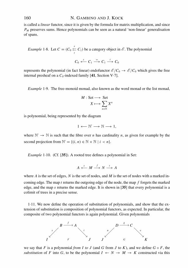
is called a linear functor, since it is given by the formula for matrix multiplication, and sincePM preserves sums. Hence polynomials can be seen as a natural ‘non-linear’ generalisationof spans.
Example 1·8. Let C = (C0
s⇔
tC1) be a category object in E . The polynomial
C0s←− C1
=−→ C1t−→ C0
represents the polynomial (in fact linear) endofunctor E /C0 → E /C0 which gives the freeinternal presheaf on a C0-indexed family [41, Section V·7].
Example 1·9. The free-monoid monad, also known as the word monad or the list monad,
M : Set −→ Set
X �−→∑n∈N
Xn
is polynomial, being represented by the diagram
1 ←− N′ −→ N −→ 1,
where N′ → N is such that the fibre over n has cardinality n, as given for example by the
second projection from N′ = {(i, n) ∈ N × N | i < n}.
Example 1·10. (Cf. [35]). A rooted tree defines a polynomial in Set:
As←− M
f−→ Nt−→ A
where A is the set of edges, N is the set of nodes, and M is the set of nodes with a marked in-
coming edge. The map t returns the outgoing edge of the node, the map f forgets the markededge, and the map s returns the marked edge. It is shown in [35] that every polynomial is acolimit of trees in a precise sense.
1·11. We now define the operation of substitution of polynomials, and show that the ex-tension of substitution is composition of polynomial functors, as expected. In particular, thecomposite of two polynomial functors is again polynomial. Given polynomials
Bf
��
s
������
���
At
����
����
�
I F J
Dg
��
u
������
���
Cv
J G K
we say that F is a polynomial from I to J (and G from J to K ), and we define G ◦ F , thesubstitution of F into G, to be the polynomial I ← N → M → K constructed via this
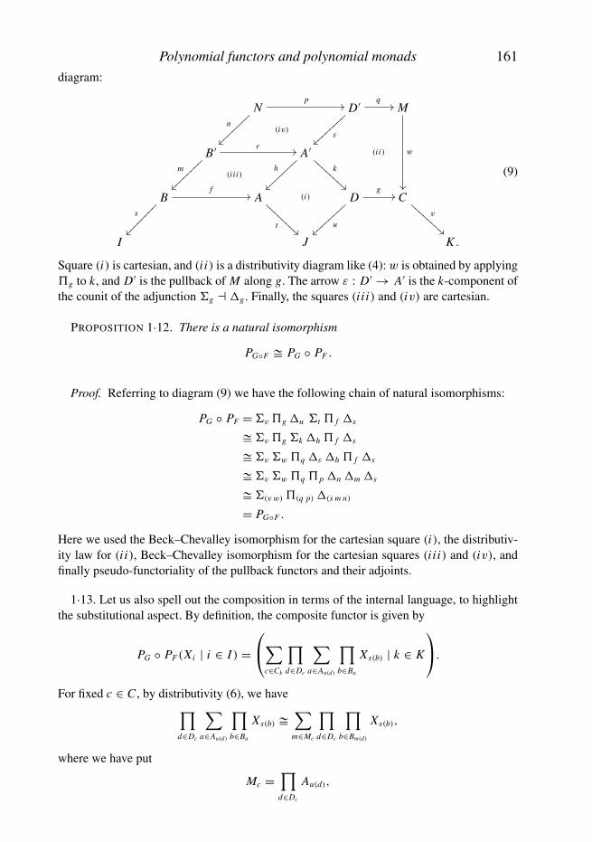
Polynomial functors and polynomial monads 161
diagram:
Nn
p��
(iv)
D′
ε
q��
(i i)
M
w
��
B ′m
����
����
r ��
(i i i)
A′k
��
����
��h
(i)Bf
��
s
������
����
A
t
����
����
D
u
g�� C
v
���
����
�
I J K .
(9)
Square (i) is cartesian, and (i i) is a distributivity diagram like (4): w is obtained by applying�g to k, and D′ is the pullback of M along g. The arrow ε : D′ → A′ is the k-component ofthe counit of the adjunction �g � �g. Finally, the squares (i i i) and (iv) are cartesian.
PROPOSITION 1·12. There is a natural isomorphism
PG◦F � PG ◦ PF .
Proof. Referring to diagram (9) we have the following chain of natural isomorphisms:
PG ◦ PF = �v �g �u �t � f �s
��v �g �k �h � f �s
��v �w �q �ε �h � f �s
��v �w �q �p �n �m �s
��(v w) �(q p) �(s m n)
= PG◦F .
Here we used the Beck–Chevalley isomorphism for the cartesian square (i), the distributiv-ity law for (i i), Beck–Chevalley isomorphism for the cartesian squares (i i i) and (iv), andfinally pseudo-functoriality of the pullback functors and their adjoints.
1·13. Let us also spell out the composition in terms of the internal language, to highlightthe substitutional aspect. By definition, the composite functor is given by
PG ◦ PF(Xi | i ∈ I ) =⎛⎝∑
c∈Ck
∏d∈Dc
∑a∈Au(d)
∏b∈Ba
Xs(b) | k ∈ K
⎞⎠.
For fixed c ∈ C , by distributivity (6), we have∏d∈Dc
∑a∈Au(d)
∏b∈Ba
Xs(b) �∑
m∈Mc
∏d∈Dc
∏b∈Bm(d)
Xs(b),
where we have put
Mc =∏
d∈Dc
Au(d),

162 N. GAMBINO AND J. KOCK
the w-fibre over c in diagram (9). If we also put, for m ∈ Mc,
N(c,m) =∑d∈Dc
Bm(d),
the (q ◦ p)-fibre over m ∈ Mc, we can write∑m∈Mc
∏d∈Dc
∏b∈Bm(d)
Xs(b) �∑
m∈Mc
∏(d,b)∈N(c,m)
Xs(b).
Summing now over c ∈ Ck , for k ∈ K , we conclude
PG ◦ PF(Xi | i ∈ I )�
⎛⎝ ∑(c,m)∈Mk
∏(d,b)∈N(c,m)
Xs(b) | k ∈ K
⎞⎠ ,
(where Mk = ∑c∈Ck
Mc is the (v ◦ w)-fibre over k ∈ K ).
COROLLARY 1·14. The class of polynomial functors is the smallest class of functorsbetween slices of E containing the pullback functors and their adjoints, and closed undercomposition and natural isomorphism.
PROPOSITION 1·15. Polynomial functors have a natural strength.
Proof. Pullback functors and their adjoints have a canonical strength.
PROPOSITION 1·16. Polynomial functors preserve connected limits. In particular, theyare cartesian.
Proof. Given a diagram as in (8), the functors �s : E /I → E /B and � f : E /B → E /Apreserve all limits since they are right adjoints. A direct calculation shows that also thefunctor �t : E /A → E /J preserves connected limits [13].
1·17. In this paper we have chosen to work with locally cartesian closed categories, sinceit is the most natural generality for the theory. However, large parts of the theory makesense also over cartesian closed categories, by considering only polynomials for which the‘middle map’ f : B → A is exponentiable, or belongs to a subclass of the exponentiablemaps having the same stability properties to ensure that Beck–Chevalley, distributivity, andcomposition of polynomial functors work just as in the locally cartesian closed case. Furtherresults about polynomial functors in this generality can be deduced from the locally cartesianclosed theory by way of the Yoneda embedding y : E → E , where E denotes the categoryof presheaves on E with values in a category of sets so big that E is small relatively to it.The Yoneda embedding is compatible with slicing and preserves the three basic operations,so that basic results about polynomial functors in E can be proved by reasoning in E . Asignificant example of this situation is the cartesian closed category of compactly generatedHausdorff spaces, where for example the covering maps constitute a stable class of expo-nentiable maps. Polynomial functors in this setting were used by Bisson and Joyal [10] togive a geometric construction of Dyer–Lashof operations in bordism. Another example isthe category of small categories, where the Conduche fibrations are the exponentiable maps.In this setting, an example of a polynomial functor is the family functor, associating to acategory X the category of families of objects in X .
Polynomial functors and polynomial monads 163
1·18. For the remainder of this section, with the aim of putting the theory of polynomialfunctors in historical perspective, we digress into the special case E = Set, then make someremarks on finitary polynomial functors, and end with finite polynomials. This material isnot needed in the subsequent sections.
The case E = Set is somewhat special due to the equivalence Set/I � SetI , which allowsfor various equivalent characterisations of polynomial functors over Set.
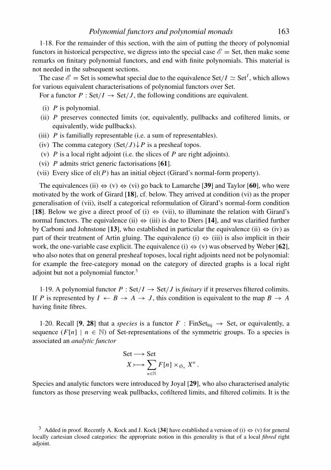
For a functor P : Set/I → Set/J , the following conditions are equivalent.
(i) P is polynomial.(ii) P preserves connected limits (or, equivalently, pullbacks and cofiltered limits, or
equivalently, wide pullbacks).(iii) P is familially representable (i.e. a sum of representables).(iv) The comma category (Set/J )↓P is a presheaf topos.(v) P is a local right adjoint (i.e. the slices of P are right adjoints).
(vi) P admits strict generic factorisations [61].(vii) Every slice of el(P) has an initial object (Girard’s normal-form property).
The equivalences (ii) ⇔ (v) ⇔ (vi) go back to Lamarche [39] and Taylor [60], who weremotivated by the work of Girard [18], cf. below. They arrived at condition (vi) as the propergeneralisation of (vii), itself a categorical reformulation of Girard’s normal-form condition[18]. Below we give a direct proof of (i) ⇔ (vii), to illuminate the relation with Girard’snormal functors. The equivalence (ii) ⇔ (iii) is due to Diers [14], and was clarified furtherby Carboni and Johnstone [13], who established in particular the equivalence (ii) ⇔ (iv) aspart of their treatment of Artin gluing. The equivalence (i) ⇔ (iii) is also implicit in theirwork, the one-variable case explicit. The equivalence (i) ⇔ (v) was observed by Weber [62],who also notes that on general presheaf toposes, local right adjoints need not be polynomial:for example the free-category monad on the category of directed graphs is a local rightadjoint but not a polynomial functor.3
1·19. A polynomial functor P : Set/I → Set/J is finitary if it preserves filtered colimits.If P is represented by I ← B → A → J , this condition is equivalent to the map B → Ahaving finite fibres.
1·20. Recall [9, 28] that a species is a functor F : FinSetbij → Set, or equivalently, asequence (F[n] | n ∈ N) of Set-representations of the symmetric groups. To a species isassociated an analytic functor
Set −→ Set
X �−→∑n∈N
F[n] ×Sn Xn .
Species and analytic functors were introduced by Joyal [29], who also characterised analyticfunctors as those preserving weak pullbacks, cofiltered limits, and filtered colimits. It is the
3 Added in proof. Recently A. Kock and J. Kock [34] have established a version of (i) ⇔ (v) for generallocally cartesian closed categories: the appropriate notion in this generality is that of a local fibred rightadjoint.
164 N. GAMBINO AND J. KOCK
presence of group actions that makes the preservation of pullbacks weak, in contrast to thepolynomial functors, cf. (ii) above. Species for which the group actions are free are called flatspecies [9]; they encode rigid combinatorial structures, and correspond to ordinary generat-ing functions rather than exponential ones. The analytic functor associated to a flat speciespreserves pullbacks strictly and is therefore the same thing as a finitary polynomial functoron Set. Explicitly, given a one-variable finitary polynomial functor P(X) = ∑
a∈A X Ba rep-resented by B → A, we can ‘collect terms’: let An denote the set of fibres of cardinality n,then there is a bijection ∑
a∈A
X Ba �∑n∈N
An × Xn.
The involved bijections Ba � n are not canonical: the degree-n part of P is rather a Sn-torsor, denoted P[n], and we can write instead
P(X)�∑n∈N
P[n] ×Sn Xn, (10)
which is the analytic expression of P .As an example of the polynomial encoding of a flat species, consider the species C of
binary planar rooted trees. The associated analytic functor is
X �→∑n∈N
C[n] ×Sn Xn ,
where C[n] is the set of ways to organise an n-element set as the set of nodes of abinary planar rooted tree; C[n] has cardinality n! cn , where cn are the Catalan numbers1, 1, 2, 5, 14, . . . The polynomial representation is
1 ←− B −→ A −→ 1
where A is the set of isomorphism classes of binary planar rooted trees, and B is the set ofisomorphism classes of binary planar rooted trees with a marked node.
1·21. Girard [18], aiming at constructing models for lambda calculus, introduced the no-tion of normal functor: it is a functor SetI → SetJ which preserves pullbacks, cofilteredlimits and filtered colimits, i.e. a finitary polynomial functor. Girard’s interest was a certainnormal-form property (reminiscent of Cantor’s normal form for ordinals), which in modernlanguage is (vii) above: the normal forms of the functor are the initial objects of the slices ofits category of elements. Girard, independently of [29], also proved that these functors admita power series expansion, which is just the associated (flat) analytic functor. From Girard’sproof we can extract in fact a direct equivalence between (i) and (vii) (independent of thefiniteness condition). The proof shows that, in a sense, the polynomial representation is thenormal form. For simplicity we treat only the one-variable case.
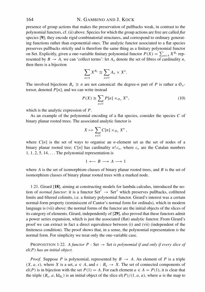
PROPOSITION 1·22. A functor P : Set → Set is polynomial if and only if every slice ofel(P) has an initial object.
Proof. Suppose P is polynomial, represented by B → A. An element of P is a triple(X, a, s), where X is a set, a ∈ A, and s : Ba → X . The set of connected components ofel(P) is in bijection with the set P(1) = A. For each element a ∈ A = P(1), it is clear thatthe triple (Ba, a, IdBa ) is an initial object of the slice el(P)/(1, a, u), where u is the map to

Polynomial functors and polynomial monads 165
the terminal object. These initial objects induce initial objects in all the slices, since everyelement (X, a, s) has a unique map to (1, a, u).
Conversely, suppose every slice of el(P) has an initial object; again we only need theinitial objects of the special slices el(P)/(1, a, u), for a ∈ P(1). Put A = P(1). It remainsto construct B over A and show that the resulting polynomial functor is isomorphic to P .Denote by (Ba, b) the initial object of el(P)/(1, a, u). Let now X be any set. The uniquemap X → 1 induces P(X) → P(1) = A, and we denote by P(X)a the preimage of a. Foreach element x ∈ P(X)a , the pair (X, x) is therefore an object of the slice el(P)/(1, a, u),so by initiality we get a map Ba → X . Conversely, given any map α : Ba → X , define xto be the image under P(α) of the element b; clearly x ∈ P(X)a . These two constructionsare easily checked to be inverse to each other, establishing a bijection P(X)a � X Ba . Thesebijections are clearly natural in X , and since P(X) = ∑
a∈A P(X)a we conclude that P isisomorphic to the polynomial functor represented by the projection map
∑a∈A Ba → A.
1·23. Call a polynomial over Set
I ←− B −→ A −→ J (11)
finite if the four involved sets are finite. Clearly the composite of two finite polynomials isagain finite. The category T whose objects are finite sets and whose morphisms are the finitepolynomials (up to isomorphism) was studied by Tambara [59], in fact in the more gen-eral context of finite G-sets, for G a finite group. His paper is probably the first to displayand give emphasis to diagrams like (11). Tambara was motivated by representation theoryand group cohomology, where the three operations �, �, � are, respectively, ‘restriction’,‘trace’ (additive transfer), and ‘norm’ (multiplicative transfer). We shall not go into theG-equivariant achievements of [59], but wish to point out that the following fundamentalresult about polynomial functors is implicit in Tambara’s paper and should be attributed tohim.
THEOREM 1·24. The skeleton of T is the Lawvere theory for commutative semirings.
The point is firstly that m + n is the product of m and n in T (this is most easily seen byextension, where it amounts to Set/(m + n) � Set/m × Set/n). And secondly that for thetwo Set-maps
0e−→ 1
m←− 2
the polynomial functor �m , considered as a map in T, represents addition, �m representsmultiplication, and �e and �e represent the additive and multiplicative neutral elements,respectively. Pullback provides the projection for the product in T, and is also needed toaccount for distributivity, which in syntactic terms involves duplicating elements. It is abeautiful exercise to use the abstract distributive law (5) to compute
�m ◦ �k
where k : 3 → 2 is the map pictured as , recovering the distributive law a(x + y) =ax + ay of elementary algebra.
2. Morphisms of polynomial functors
Since polynomial functors have a canonical strength, the natural notion of morphismbetween polynomial functors is that of strong natural transformation. We shall see that
166 N. GAMBINO AND J. KOCK
strong natural transformations between polynomial functors are uniquely represented bycertain diagrams connecting the polynomials.
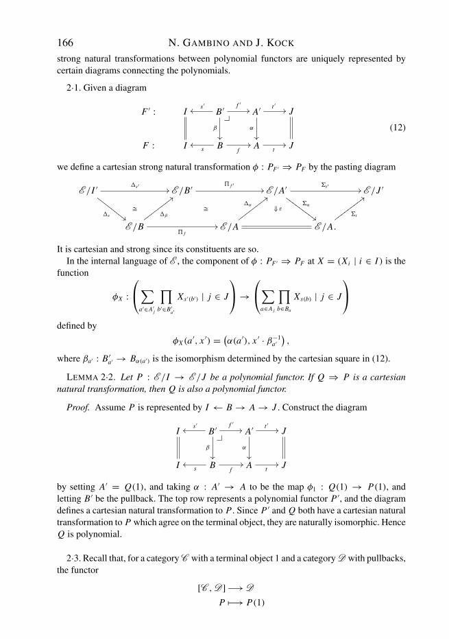
2·1. Given a diagram
F ′ : I B ′��
f ′��s ′
��
β
��
A′ t ′��
α
��
J
F : I Bf
��s
�� A t�� J
(12)
we define a cartesian strong natural transformation φ : PF ′ ⇒ PF by the pasting diagram
E /I ′ �s′ ��
�s ����������
�
E /B ′ � f ′��
�
E /A′
⇓ ε
�t ′ ��
�α
������
����
� E /J ′
E /B� f
��
�β
����������E /A
�α
����������E /A.
�t
�����������
It is cartesian and strong since its constituents are so.In the internal language of E , the component of φ : PF ′ ⇒ PF at X = (Xi | i ∈ I ) is the
function
φX :⎛⎝ ∑
a′∈A′j
∏b′∈B ′
a′
Xs ′(b′) | j ∈ J
⎞⎠ →⎛⎝∑
a∈A j
∏b∈Ba
Xs(b) | j ∈ J
⎞⎠defined by
φX (a′, x ′) = (α(a′), x ′ · β−1
a′),
where βa′ : B ′a′ → Bα(a′) is the isomorphism determined by the cartesian square in (12).
LEMMA 2·2. Let P : E /I → E /J be a polynomial functor. If Q ⇒ P is a cartesiannatural transformation, then Q is also a polynomial functor.
Proof. Assume P is represented by I ← B → A → J . Construct the diagram
I B ′��
f ′��s ′
��
β
��
A′ t ′��
α
��
J
I Bf
��s
�� A t�� J
by setting A′ = Q(1), and taking α : A′ → A to be the map φ1 : Q(1) → P(1), andletting B ′ be the pullback. The top row represents a polynomial functor P ′, and the diagramdefines a cartesian natural transformation to P . Since P ′ and Q both have a cartesian naturaltransformation to P which agree on the terminal object, they are naturally isomorphic. HenceQ is polynomial.
2·3. Recall that, for a category C with a terminal object 1 and a category D with pullbacks,the functor
[C ,D] −→ D
P �−→ P(1)
Polynomial functors and polynomial monads 167
is a Grothendieck fibration. The cartesian arrows for this fibration are precisely the cartesiannatural transformations, while the vertical arrows are the natural transformations whosecomponent on 1 is an identity map. We refer to such natural transformations as verticalnatural transformations.
If C and D are enriched and tensored, then the above remark carries over to the casewhere [C ,D] denotes the category of strong functors and strong natural transformations.The verification of this involves observing that the cartesian lift of a strong functor has acanonical strength.
PROPOSITION 2·4. Let I, J ∈ E . The restriction of the Grothendieck fibration
[E /I,E /J ] −→ E /J
P �−→ P(1)
to the category of polynomial functors and strong natural transformations is again aGrothendieck fibration.
Proof. Lemma 2·2 implies that the cartesian lift of a polynomial functor is again polyno-mial.
2·5. Proposition 2·4 implies that every strong natural transformation between polynomialfunctors factors in an essentially unique way as a vertical strong natural transformation fol-lowed by a cartesian one. We proceed to establish representations of the two classes of strongnatural transformations between polynomial functors. The key ingredient is the followingversion of the enriched Yoneda lemma.
LEMMA 2·6. Let u : I → 1 denote the unique arrow in E to the terminal object. For anys : B → I and s ′ : B ′ → I in E /I , the natural map
Hom E /I (s, s ′) −→ StrNat(�u�s ′�s ′, �u�s�s)
sending an I -map w : B → B ′ to the composite �u�s ′�s ′η⇒ �u�s ′�w�w�s ′ ��u�s�s
is a bijection.
Proof. Just note that �u�s�s = Hom E /I (s, −) : E /I → E , and the result is the usualenriched Yoneda lemma [31], remembering that since E /I is tensored over E , a naturaltransformation (between strong functors) is enriched if and only if it is strong.
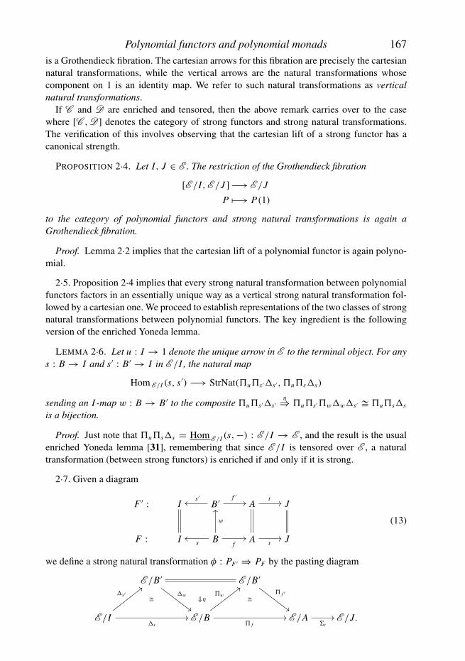
2·7. Given a diagram
F ′ : I B ′ f ′��s ′
�� At �� J
F : I Bf
��
w
s�� A t
�� J
(13)
we define a strong natural transformation φ : PF ′ ⇒ PF by the pasting diagram
E /B ′
�w
����������
� ⇓η
E /B ′
�� f ′
����������
E /I
�s′����������
�s
�� E /B
�w
����������
� f
�� E /A�t
�� E /J.
168 N. GAMBINO AND J. KOCK
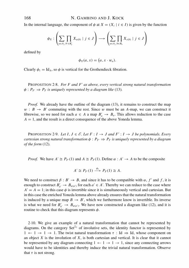
In the internal language, the component of φ at X = (Xi | i ∈ I ) is given by the function
φX :⎛⎝∑
a∈A j
∏b′∈B ′
a
Xu(b) | j ∈ J
⎞⎠ −→⎛⎝∑
a∈A j
∏b∈Ba
Xs(b) | j ∈ J
⎞⎠defined by
φX (a, x) = (a, x · wa).
Clearly φ1 = IdA, so φ is vertical for the Grothendieck fibration.
PROPOSITION 2·8. For F and F ′ as above, every vertical strong natural transformationφ : PF ′ ⇒ PF is uniquely represented by a diagram like (13).
Proof. We already have the outline of the diagram (13), it remains to construct the mapw : B → B ′ commuting with the rest. Since w must be an A-map, we can construct itfibrewise, so we need for each a ∈ A a map B ′
a → Ba . This allows reduction to the caseA = 1, and the result is a direct consequence of the above Yoneda lemma.
PROPOSITION 2·9. Let I, J ∈ E . Let F : I → J and F ′ : I → J be polynomials. Everycartesian strong natural transformation φ : PF ′ ⇒ PF is uniquely represented by a diagramof the form (12).
Proof. We have A′ � PF ′(1) and A � PF(1). Define α : A′ → A to be the composite
A′ � PF ′(1)φ1−→ PF(1)� A.
We need to construct β : B ′ → B, and since it has to be compatible with α, f ′ and f , it isenough to construct B ′
a′ → Bα(a′) for each a′ ∈ A′. Thereby we can reduce to the case whereA′ = A = 1; in this case φ is invertible since it is simultaneously vertical and cartesian. Butin this case the enriched Yoneda lemma above already ensures that the natural transformationis induced by a unique map B → B ′, which we furthermore know is invertible. Its inverseis what we need for B ′
a′ → Bα(a′). We have now constructed a diagram like (12), and it isroutine to check that this diagram represents φ.
2·10. We give an example of a natural transformation that cannot be represented bydiagrams. On the category SetZ2 of involutive sets, the identity functor is represented by1 ← 1 → 1 → 1. The twist natural transformation τ : Id ⇒ Id, whose component onan object X is the involution of X , is both cartesian and vertical. It is clear that it cannotbe represented by any diagram connecting 1 ← 1 → 1 → 1, since any connecting arrowswould have to be identities and thereby induce the trivial natural transformation. Observethat τ is not strong.

Polynomial functors and polynomial monads 169
2·11. We can now combine the diagrams representing vertical and cartesian strong naturaltransformations. Given a diagram
G : I Dg
��u�� Cv �� J
B ′ ��
��
�� C
��
F : I Bf
��s
�� A t�� J
(14)
there is induced, by (2·1) and (2·7), a strong natural transformation Pφ : PG ⇒ PF . Werefer to a diagram like (14) as a morphism from G to F . We arrive at the following result,a version of which appears as [2, theorem 3·4], where it is stated for polynomial functorsbetween slice categories over discrete objects.
THEOREM 2·12. Every strong natural transformation PG ⇒ PF between polynomialfunctors is represented in an essentially unique way by a diagram like (14).
Proof. By Proposition 2·4, every strong natural transformation factors as a vertical strongtransformation followed by a cartesian strong natural transformation in an essentially uniqueway. The claim then follows from Proposition 2·8 and Proposition 2·9.
COROLLARY 2·13. Every strong natural transformation between polynomial functors isa composite of units and counits of the basic adjunctions, their inverses when they exist, andcoherence 2-cells for pullback and its adjoints.
Proof. The ingredients of the constructions in (2·1) and (2·7) are units, counits, pseudo-functoriality 2-cells, as well as Beck-Chevalley isomorphisms, which in turn are constructedusing units and counits (and inverses of their composites).
2·14. Polynomials from I to J and their morphisms form a category denoted PolyE (I, J ).Vertical composition of diagrams like (14) involves a simple pullback construction thatvia extension amounts precisely to refactoring cartesian-followed-by-vertical into vertical-followed-by-cartesian, cf. the fibration property. This can also be described as the uniqueway of defining vertical composition of diagrams to make the assignment given by exten-sion functorial. If we let PolyFunE (E /I,E /J ) denote the category of polynomial functorsfrom E /I to E /J and strong natural transformations, we can reformulate Theorem 2·12 asfollows.
LEMMA 2·15. For any I, J , the functor given by extension,
Ext : PolyE (I, J ) −→ PolyFunE (E /I,E /J ) ,
is an equivalence of categories.
2·16. The involved categories are hom categories of appropriate bicategories of polyno-mials and polynomial functors, respectively, that we now describe, assembling the equival-ences of the lemma into a biequivalence of bicategories (2·17). We define the 2-category ofpolynomial functors PolyFunE as the sub-2-category of Cat having slices of E as 0-cells,polynomial functors as 1-cells, and strong natural transformations as 2-cells.

170 N. GAMBINO AND J. KOCK
We shall describe a bicategory PolyE which has objects of E as 0-cells, polynomials as1-cells, and whose 2-cells are the morphisms of polynomials, i.e. diagrams like (14). Thevertical composition of 2-cells has already been described, as has the horizontal compositionof 1-cells. To define the horizontal composition of 2-cells we simply transport back the 2-cellstructure from PolyFunE along the local equivalences of Lemma 2·15.
We begin by extending the family of functions mapping a pair of composable polynomialsF and G to their composite G ◦ F , which we defined in Paragraph (1·11), to a family offunctors
PolyE (J, K ) × PolyE (I, J ) −→ PolyE (I, K ) .
For this, let φ : F ⇒ F ′ be a morphism between polynomials from I to J , and let ψ :G ⇒ G ′ be a morphism between polynomials from J to K . We define the morphism ψ ◦φ :G ◦ F ⇒ G ′ ◦ F ′ as the unique morphism of polynomials making the following diagramcommute
P(G ◦ F)P(ψ◦φ)
��
αG,F
��
P(G ′ ◦ F ′)
αG′ ,F ′��
P(G) P(F)P(ψ) P(φ)
�� P(G ′) P(F ′) .
Here αG,F and αG ′,F ′ are instances of the isomorphism of Theorem 1·12, and the diagramnow expresses the naturality of α. We therefore get the following natural isomorphism offunctors
PolyE (J, K ) × PolyE (I, J ) ��
�PJ,K ×PI,J
��
PolyE (I, K )
PI,K
��
PolyFunE (E /J,E /K ) × PolyFunE (E /I,E /J ) �� PolyFunE (E /I,E /K )
where the top horizontal functor is substitution of polynomials and the bottom horizontalmap is composition of functors in PolyFunE . The identity maps in PolyE are represented bythe polynomials IdI : I → I , and we have natural isomorphisms
PolyE (I, I )
PI,I
��
1
IdI
���������������
1E /I��������������� �
PolyFunE (E /I,E /I ) .
We define the associativity and unit isomorphisms. For associativity, given polynomials F :I → J , G : J → K , and H : K → L , define
θH,G,F : (H ◦ G) ◦ F =⇒ H ◦ (G ◦ F)

Polynomial functors and polynomial monads 171
to be the unique morphism of polynomials making the following diagram commute
P((H ◦ G) ◦ F)P(θH,G,F )
��
αH◦G,F
��
P(H ◦ (G ◦ F))
αH,G◦F
��
P(H ◦ G) P(F)
αH,G P(F)
��
P(H) P(G ◦ F)
P(H) αG,F
��(P(H) P(G)
)P(F) P(H)
(P(G) P(F)
).
(15)
For the unit isomorphisms, given a polynomial F : I → J , define
λF : IdJ ◦ F =⇒ F , ρF : F ◦ IdI =⇒ F
to be the unique morphism of polynomials such that
P(IdJ ◦ F)P(λF )
��
αIdJ ,F
��
P(F)
P(IdJ ) P(F)αJ P(F)
�� 1E /J P(F)
(16)
and
P(F ◦ IdI )P(ρF )
��
φF,IdI
��
P(F)
P(F) P(IdI ) P(F) αI
�� P(F) 1E /I
(17)
commute. All the data of the bicategory PolyE have now been given. The naturality andcoherence axioms for a bicategory can be verified by standard diagram-chasing arguments,which exploit the uniqueness properties used to define the components of θ , λ, and ρ. Theinterchange law of PolyFunE is used at several points. Let us remark that the definition ofthe bicategory PolyE is essentially determined by the requirement that we obtain a pseudo-functor
Ext : PolyE −→ PolyFunE .
Indeed, the diagrams in (15), (16), (17) express exactly the coherence conditions for apseudo-functor [8]. It is clear by construction that this pseudo-functor is bijective on objects,and it is locally an equivalence of categories by Lemma 2·15. Hence we have established thefollowing.
THEOREM 2·17. The extension pseudo-functor
Ext : PolyE −→ PolyFunE
is a biequivalence.
2·18. The notions of polynomial and polynomial functors are almost exactly the same aswhat is called container and container functor by Abbott, Altenkirch and Ghani [1, 2, 3, 4].One minor difference is that they only consider slices over discrete objects, i.e. of the formE /n � E n , where n denotes the sum of n copies of the terminal object, and for this they

172 N. GAMBINO AND J. KOCK
also need to assume finite sums. In our setting there is no reason for that restriction, and infact Altenkirch and Morris [5] have been able to lift the restriction also from the containertheory, introducing the notion of indexed container. Another difference, also quite minor,is that while we prefer to work with strength, the literature on containers considers fibredcategories, fibred functors and fibred natural transformations. This involves replacing allslice categories E /I by the fibration over E whose K -fibre is E /(K × I ), and work withthose instead. The two viewpoints are in fact equivalent, thanks to a result of Pare, whoshowed (cf. [27]) that if a strong functor preserves pullbacks then it is canonically indexed,i.e. fibred. (It is easy to see that a fibred functor has a strength.) We have chosen the viewpointof tensorial strength for its simplicity. Modulo the above minor differences (and moduloPare’s theorem), Lemma 2·2, Theorem 2·12, and Theorem 2·17 were also proved in Abbott’sthesis [1].
3. The double category of polynomial functors
3·1. It is important to be able to compare polynomial functors with different endpoints,and to base change polynomial functors along maps in E . This need can been seen alreadyfor linear functors 1·7: a small category is a monad in the bicategory of spans [8], but inorder to get functors between categories with different object sets, one needs maps betweenspans with different endpoints [38]. The most convenient framework for this is that of doublecategories, as it allows for diagrammatic representation. The base change structure is con-cisely captured in Shulman’s notion of framed bicategory [55]: our double categories ofpolynomial functors will in fact be framed bicategories.
3·2. Recall that a double category D consists of a category of objects D0, a category ofmorphisms D1, together with structure functors
D0�� D1
∂0
��
∂1��D1 ×D0 D1
comp.��
subject to the usual category axioms. The objects of D0 are called objects of D, the morph-isms of D0 are called vertical arrows, the objects of D1 are called horizontal arrows, andthe morphisms of D1 are called squares. As is custom [19], we allow the possibility for thehorizontal composition to be associative and unital only up to specified coherent isomorph-isms. Precisely, a double category is a pseudo-category [47] in the 2-category Cat; see also[43, Section 5·2].
3·3. A framed bicategory [55] is a double category for which the functor
(∂0, ∂1) : D1 −→ D0 × D0
is a bifibration. (In fact, if it is a fibration then it is automatically an opfibration, and viceversa.) The upshot of this condition is that horizontal arrows can be base changed and cobasechanged along arrows in D0 × D0 (i.e. pairs of vertical arrows).
3·4. We need to fix some terminology. The characteristic property of a fibration is thatevery arrow in the base category admits a cartesian lift, and that every arrow in the totalspace factors (essentially uniquely) as a vertical arrow followed by a cartesian one. In thepresent situation, the term ‘cartesian’ is already in use to designate cartesian natural trans-formations (which fibrationally speaking are vertical rather than cartesian), and the word
Polynomial functors and polynomial monads 173
‘vertical’ already has a double-categorical meaning. For these reasons, instead of talkingabout ‘cartesian arrow’ for a fibration we shall say transporter arrow; this terminologygoes back to Grothendieck [20]. Correspondingly, we shall say cotransporter instead ofopcartesian. We shall simply refrain from using ‘vertical’ in the fibration sense. The arrowsmapping to identity arrows by the fibration will be precisely the natural transformations ofpolynomial functors.
3·5. We want to extend the bicategories PolyE and PolyFunE to double categories. Theobjects of the double category PolyFunE are the slices of E , and the horizontal arrows arethe polynomial functors. The vertical arrows are the dependent sum functors (i.e. functorsof the form �u for some u), and the squares in PolyE are of the form
E /I ′
�u
��
P ′��
⇓ φ
E /J ′
�v
��
E /IP
�� E /J
(18)
where P ′ and P are polynomial functors and φ is a strong natural transformation.
PROPOSITION 3·6. The double category PolyFunE is a framed bicategory.
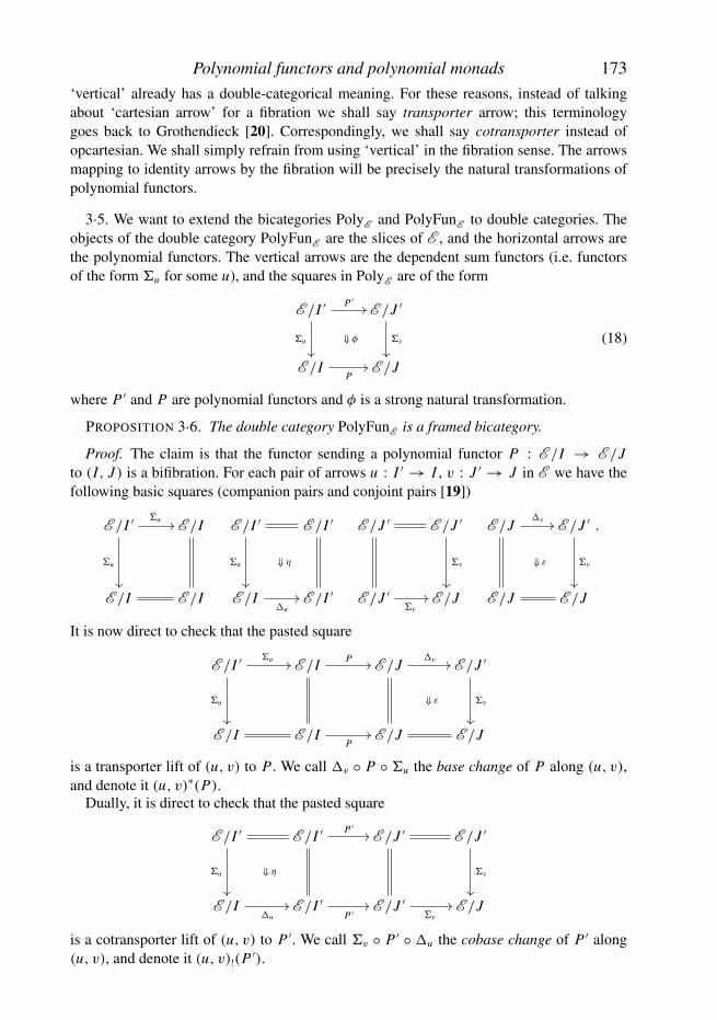
Proof. The claim is that the functor sending a polynomial functor P : E /I → E /Jto (I, J ) is a bifibration. For each pair of arrows u : I ′ → I , v : J ′ → J in E we have thefollowing basic squares (companion pairs and conjoint pairs [19])
E /I ′ �u ��
�u
��
E /I
E /I E /I
E /I ′
�u
��
⇓ η
E /I ′
E /I�u
�� E /I ′
E /J ′ E /J ′
�v
��
E /J ′�v
�� E /J
E /J�v ��
⇓ ε
E /J ′
�v
��
E /J E /J
.
It is now direct to check that the pasted square
E /I ′ �u ��
�u
��
E /I P �� E /J�v ��
⇓ ε
E /J ′
�v
��
E /I E /IP
�� E /J E /J
is a transporter lift of (u, v) to P . We call �v ◦ P ◦ �u the base change of P along (u, v),and denote it (u, v)∗(P).
Dually, it is direct to check that the pasted square
E /I ′
�u
��
⇓ η
E /I ′ P ′�� E /J ′ E /J ′
�v
��
E /I�u
�� E /I ′P ′
�� E /J ′�v
�� E /J
is a cotransporter lift of (u, v) to P ′. We call �v ◦ P ′ ◦ �u the cobase change of P ′ along(u, v), and denote it (u, v)!(P ′).

174 N. GAMBINO AND J. KOCK
The above procedure of getting a framed bicategory out of a bicategory is a general con-struction: one starts with a bicategory C with a subcategory L consisting of left adjointsand comprising all the objects of C , and obtains a framed bicategory by taking as verticalarrows the arrows in L . The details can be found in [55, appendix].
3·7. Via the biequivalence PolyE � PolyFunE between the bicategory of polynomials andthe 2-category of polynomial functors, Proposition 3·6 gives us also a framed bicategory ofpolynomials PolyE , featuring nice diagrammatic representations which we now spell out,extending the results of Section 2. The following result is the double-category version ofTheorem 2·12.
THEOREM 3·8. The squares (18) of PolyFunE are represented by diagrams of the form
P ′ : I ′
u
��
B ′�� �� A′ �� J ′
v
��
·��
��
��
·
��
P : I B�� �� A �� J .
(19)
This representation is unique up to choice of pullback in the middle. It follows that extensionconstitutes a framed biequivalence
PolyE∼→ PolyFunE .
Proof. By Theorem 2·12, diagrams like (19) (up to choice of pullback) are in bijectivecorrespondence with strong natural transformations �v ◦ P ′ ◦�u ⇒ P , which by adjointnesscorrespond to strong natural transformations �v◦P ′ ⇒ P◦�u , i.e. squares (18) in PolyFunE .
3·9. The vertical composition of two diagrams
·
��
·�� �� · �� ·
��
·��
��
��
·
��·
��
·�� �� · �� ·
��
·��
��
��
·
��· ·�� �� · �� ·is performed by replacing the two middle squares
·�� ��
��
·
��· �� ·
·
�� ·
Polynomial functors and polynomial monads 175
by a configuration
· �� ·
·�� ��
��
·
��· �� ·and then composing vertically. The replacement is a simple pullback construction, andchecking that the composed diagram has the same extension as the vertical pasting of theextensions is a straightforward calculation.
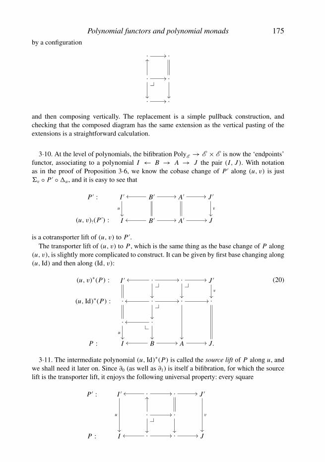
3·10. At the level of polynomials, the bifibration PolyE → E × E is now the ‘endpoints’functor, associating to a polynomial I ← B → A → J the pair (I, J ). With notationas in the proof of Proposition 3·6, we know the cobase change of P ′ along (u, v) is just�v ◦ P ′ ◦ �u , and it is easy to see that
P ′ : I ′
u
��
B ′�� �� A′ �� J ′
v
��
(u, v)!(P ′) : I B ′�� �� A′ �� J
is a cotransporter lift of (u, v) to P ′.The transporter lift of (u, v) to P , which is the same thing as the base change of P along
(u, v), is slightly more complicated to construct. It can be given by first base changing along(u, Id) and then along (Id, v):
(u, v)∗(P) : I ′ ·��
�� ��
��
·��
��
�� J ′
v
��(u, Id)∗(P) : · ·
����
��
�� ·
��
�� ·
·u
��
·����
��
P : I B�� �� A �� J.
(20)
3·11. The intermediate polynomial (u, Id)∗(P) is called the source lift of P along u, andwe shall need it later on. Since ∂0 (as well as ∂1) is itself a bifibration, for which the sourcelift is the transporter lift, it enjoys the following universal property: every square
P ′ : I ′
u
��
·�� �� · �� J ′
v
��
·��
��
��
·
��
P : I ·�� �� · �� J
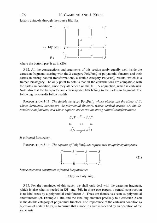
176 N. GAMBINO AND J. KOCK
factors uniquely through the source lift, like
P ′ : I ′ ·�� �� · �� J ′
v
��
·��
��
��
·
��(u, Id)∗(P) : I ′
u��
·����
��
�� ·
��
�� ·
P : I ·�� �� · �� J
where the bottom part is as in (20).
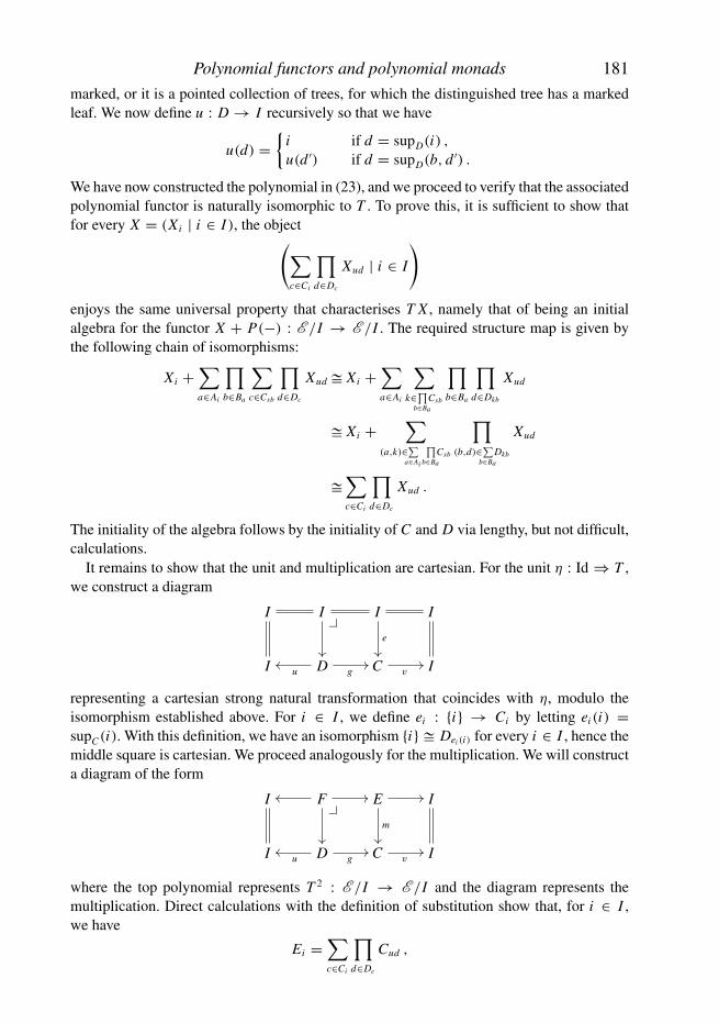
3·12. All the constructions and arguments of this section apply equally well inside thecartesian fragment: starting with the 2-category PolyFunc
E of polynomial functors and theircartesian strong natural transformations, a double category PolyFunc
E results, which is aframed bicategory. The only point to note is that all the constructions are compatible withthe cartesian condition, since they all depend on the � � � adjunction, which is cartesian.Note also that the transporter and cotransporter lifts belong to the cartesian fragment. Thefollowing two results follow readily.
PROPOSITION 3·13. The double category PolyFuncE whose objects are the slices of E ,
whose horizontal arrows are the polynomial functors, whose vertical arrows are the de-pendent sum functors, and whose squares are cartesian strong natural transformations
E /I ′
�u
��
P ′��
⇓ φ
E /J ′
�v
��
E /IP
�� E /J
is a framed bicategory.
PROPOSITION 3·14. The squares of PolyFuncE are represented uniquely by diagrams
I ′
��
B ′��
�� ��
��
A′
��
�� J ′
��
I B�� �� A �� J ,
(21)
hence extension constitutes a framed biequivalence
PolycE
∼→ PolyFuncE .
3·15. For the remainder of this paper, we shall only deal with the cartesian fragment,which is also what is needed in [35] and [36]. In those two papers, a central constructionis to label trees by a polynomial endofunctor P . Trees are themselves seen as polynomialendofunctors (cf. Example 1·10), and the labelling amounts precisely to a cartesian 2-cellin the double category of polynomial functors. The importance of the cartesian condition (abijection of certain fibres) is to ensure that a node in a tree is labelled by an operation of thesame arity.

Polynomial functors and polynomial monads 177
3·16. We finish this section with a digression on the relationship between polynomialfunctors and the shapely functors and shapely types of Jay and Cockett [25, 26], since thedouble-category setting provides some conceptual simplification of the latter notion. Wenow assume E has sums.
A shapely functor [26] is a pullback-preserving functor F : E m → E n equipped witha strength. Since, for a natural number n, the discrete power E n is equivalent to the sliceE /n, where n now denotes the n-fold sum of 1 in E , it makes sense to compare shapelyfunctors and polynomial functors. Since a polynomial functor preserves pullbacks and hasa canonical strength, it is canonically a shapely functor. It is not true that every shapelyfunctor is polynomial. For a counter example, let K be a set with a non-principal filter D ,and consider the filter-power functor
F : Set −→ Set
X �−→ colim D∈D X D ,
which preserves finite limits since it is a filtered colimit of representables. Since every en-dofunctor on Set has a canonical strength, F is a shapely functor. However, F does notpreserve all cofiltered limits, and hence, by (1·18) ((ii)) cannot be polynomial. For ex-ample, � = limD∈D D itself is not preserved. This example is apparently at odds with[2, theorem 8·3].
3·17. Let L : E → E denote the list endofunctor, L(X) = ∑n∈N
Xn , which is the sameas what we called the free-monoid monad in Example 1·9. A shapely type [26] in one vari-able is a shapely functor equipped with a cartesian strong natural transformation to L . Amorphism of shapely types is a natural transformation commuting with the structure map toL . The idea is that the shapely functor represents the template or the shape into which somedata can be inserted, while the list holds the actual data; the cartesian natural transforma-tion encodes how the data is to be inserted into the template. As emphasized in [49], thecartesian strong natural transformation is part of the structure of a shapely type. Since anyfunctor with a cartesian natural transformation to L is polynomial by Lemma 2·2, it is clearthat one-variable shapely types are essentially the same thing as one-variable polynomialendofunctors with a cartesian natural transformation to L , and that there is an equivalenceof categories between the category of shapely types and the category Polyc
E (1, 1)/L .According to Jay and Cockett [26], a shapely type in m input variables and n output vari-
ables is a shapely functor E m → E n equipped with a cartesian strong natural transformationto the functor Lm,n : E m → E n defined by
Lm,n(Xi | i ∈ m) = (L(
∑i∈m Xi ) | j ∈ n
),
and they motivate this definition by considerations on how to insert data into templates.With the double-category formalism, we can give a conceptual explanation of the formula:writing um : m → 1 and un : n → 1 for the maps to the terminal object, the functorLm,n : E m → E n is nothing but the composite
�un ◦ L ◦ �um = (um, un)∗L ,
the base change of L along (um, un). Hence we can say uniformly that a shapely type is anobject in Polyc
E /L with endpoints finite discrete objects.

178 N. GAMBINO AND J. KOCK
4. Polynomial monads
4·1. Let I ∈ E . A polynomial monad on E /I is a monad (T, η, μ) for which T is apolynomial functor and η and μ are cartesian strong natural transformations. From the pointof view of the formal theory of monads [56], a polynomial monad is a monad in the 2-category PolyFunc
E . A basic example of a polynomial monad is the free-monoid monad ofExample 1·9.
4·2. We are interested in the construction of the free monad on a polynomial endofunctor,and start by recalling from [7, 30] some general facts about free monads. Let C be a categoryand P : C → C an endofunctor. The free monad on P is a monad (T, η, μ) on C togetherwith a natural transformation α : P ⇒ T enjoying the following universal property: for anymonad (T ′, η′, μ′) on C and any natural transformation φ : P ⇒ T ′ there exists a uniquemonad morphism φ� : T ⇒ T ′ making the following diagram commute:
Pα ��
φ ��
T
φ�
��
T ′.
The following construction of the free monad on P is standard. Let P-alg denote the cat-egory of P-algebras and P-algebra morphisms. We denote P-algebras as pairs (X, supX )
where X is the underlying object, and supX : P X → X is the structure map, sometimessuppressed from the notation for brevity. If the forgetful functor U : P-alg → C has a leftadjoint, then the monad (T, η, μ) resulting from the adjunction is the free monad on P . IfC has binary sums, a necessary and sufficient condition for the existence of the left adjointto U is that, for every X ∈ C , the endofunctor X + P(−) : C → C has an initial algebra.Indeed, in that case we can construct the free monad as follows. For X ∈ C , we define T Xas the initial algebra for X + P(−) : C → C , and ηX : X → T X as the composite
Xι1−→ X + P(T X)
tX−→ T X
where ι1 is the first sum inclusion and tX is the structure map of T X as an (X + P)-algebra.Finally, since T 2 X is the initial algebra for the functor T X + P(−), we can define μX :T 2 X → T X as the unique map making the following diagram commute:
T X + P(T 2 X)T X+P(μX )
��
tT X
��
T X + P(T X)
��
T X + X + P(T X)
(1T X ,tX )
��
T 2 X μX
�� T X.
Functoriality, naturality, and the monad axioms follow readily from these definitions. Notethat the X -component of the natural transformation α : P ⇒ T is given as the composite
P XP(ηX )
�� P(T X)ι2 �� X + P(T X)
tX �� T X . (22)
4·3. Let us now return to the locally cartesian closed category E , now assumed to be ex-tensive and in particular have finite sums. Recall from [48] that E is said to have W-types

Polynomial functors and polynomial monads 179
if every polynomial functor in a single variable on E has an initial algebra. This termino-logy is motivated by the fact that initial algebras for polynomial functors in a single variableare category-theoretic counterparts of Martin–Lof’s types of wellfounded trees [51]. Everyelementary topos with a natural numbers object has W-types [48]. If E has W-types, thenevery polynomial endofunctor, not just those in a single variable, has an initial algebra [17,theorem 14]. Initial algebras for general polynomial functors are category-theoretic counter-parts of Petersson and Synek’s general tree types [52]; see also [50, chapter 16].
Henceforth, we assume that E has W-types. For any polynomial endofunctor P : E /I →E /I and any X ∈ E /I , the functors X + P(−) : E /I → E /I are again polynomial, hencehave initial algebras. Therefore every polynomial endofunctor admits a free monad.
4·4. Theorem 4·5 below asserts that the free monad on a polynomial functor is polynomial.The proof exploits the possibility of recursively defining maps out of initial algebras forpolynomial functors, and we need first to set up some notation to handle this. Let P : E /I →E /I be the polynomial functor represented by the diagram
Is←− B
f−→ At−→ I.
We regard such a diagram as a generalised many-sorted signature. This point of view is mosteasily illustrated by considering the case of E = Set. The object I provides the set of sortsof the signature. The set of terms of the signature is defined inductively by saying that wehave a term supa(x) of sort t (a) whenever a ∈ A and x = (xb | b ∈ Ba) is a family of termssuch that xb has sort s(b) for all b ∈ Ba . Such a term may be represented graphically as aone-node tree
t (a).
s(b)
xb
sup(a, x)
The incoming edges are indexed by the elements of Ba and further labelled by elements ofI , with the edge indexed by b ∈ Ba labelled by s(b) ∈ I . The outgoing edge is labelled byt (a) ∈ I . We label the node sup(a, x) if the family x = (xb | b ∈ Ba) labels its incomingedges.
Let W be the initial algebra for P , with structure map supW : PW → W . Initiality ofthe algebra means that for any other algebra (X, supX ), there exists a unique algebra mapθ : W → X , thus making the following diagram commute
PWP(θ)
��
supW
��
P X
supX
��
Wθ
�� X .
In the internal language of E , we can represent the structure map of W as the I -indexedfamily
supWi:∑a∈Ai
∏b∈Ba
Wsb → Wi .

180 N. GAMBINO AND J. KOCK
The initiality of W can be expressed by saying that there exists a unique family of mapsθi : Wi → Xi satisfying the recursive equation
θi (supWi(a, h)) = supXi
(a, (λb ∈ Ba) θsb(hb)) ,
where we employ the lambda calculus notation (λb ∈ Ba) θsb(hb) to indicate the functionBa → X sending b to θsb(hb).
THEOREM 4·5. The free monad on a polynomial endofunctor is a polynomial monad.
Proof. Let P : E /I → E /I be the polynomial endofunctor represented by
Is←− B
f−→ At−→ I,
and let (T, η, μ) be the free monad on P . We need to show that T : E /I → E /I is apolynomial functor, and that η : Id ⇒ T and μ : T 2 ⇒ T are cartesian strong naturaltransformations. We shall show that T is naturally isomorphic to the polynomial functorrepresented by the diagram
Iu←− D
g−→ Cv−→ I (23)
whose constituents we now proceed to construct. Intuitively, C is the set of wellfoundedtrees with branching profile given by the polynomial endofunctor 1 + P : E /I → E /I ,while D is the set of such trees but with a marked leaf. We construct these two objects asleast fixpoints. Put Q = 1 + P; in the internal language we have
Q(Xi | i ∈ I ) =(
{i} +∑a∈Ai
∏b∈Ba
Xsb | i ∈ I
).
Let (Ci | i ∈ I ) be the initial algebra for Q. Its structure map is given by the family ofisomorphisms
supCi: {i} +
∑a∈Ai
∏b∈Ba
Csb∼→ Ci , (24)
meaning that a Q-tree is either a trivial tree (of some type i ∈ I ) or a one-node tree whichis a term from P (that is the choice of a ∈ Ai ) and whose incoming edges are labelledby Q-trees (that is the map k : Ba → Csb). We now define the polynomial endofunctorR : E /C → E /C by letting
R(Xc | c ∈ C) = (Xc | c ∈ C
),
where
Xc ={{i} if c = sup(i) ,∑
b∈BaXkb if c = sup(a, k) .
This definition can be seen to be that of a polynomial functor using the isomorphisms in (24)and the extensivity of E . Let (Dc | c ∈ C) be the initial algebra for R. Its structure mapsconsist of the following isomorphisms:
supDsupC (i): {i} ∼→ DsupC (i) , supDsupC (a,h)
:∑b∈Ba
Dhb∼→ DsupC (a,h) .
The idea here is that a tree with a marked leaf is either a trivial tree, with the unique leaf
Polynomial functors and polynomial monads 181
marked, or it is a pointed collection of trees, for which the distinguished tree has a markedleaf. We now define u : D → I recursively so that we have
u(d) ={
i if d = supD(i) ,
u(d ′) if d = supD(b, d ′) .
We have now constructed the polynomial in (23), and we proceed to verify that the associatedpolynomial functor is naturally isomorphic to T . To prove this, it is sufficient to show thatfor every X = (Xi | i ∈ I ), the object(∑
c∈Ci
∏d∈Dc
Xud | i ∈ I
)enjoys the same universal property that characterises T X , namely that of being an initialalgebra for the functor X + P(−) : E /I → E /I . The required structure map is given bythe following chain of isomorphisms:
Xi +∑a∈Ai
∏b∈Ba
∑c∈Csb
∏d∈Dc
Xud �Xi +∑a∈Ai
∑k∈∏
b∈Ba
Csb
∏b∈Ba
∏d∈Dkb
Xud
�Xi +∑
(a,k)∈∑a∈Ai
∏b∈Ba
Csb
∏(b,d)∈∑
b∈Ba
Dkb
Xud
�∑c∈Ci
∏d∈Dc
Xud .
The initiality of the algebra follows by the initiality of C and D via lengthy, but not difficult,calculations.
It remains to show that the unit and multiplication are cartesian. For the unit η : Id ⇒ T ,we construct a diagram
I I��
��
I
e
��
I
I Du��
g�� C v
�� I
representing a cartesian strong natural transformation that coincides with η, modulo theisomorphism established above. For i ∈ I , we define ei : {i} → Ci by letting ei (i) =supC(i). With this definition, we have an isomorphism {i}� Dei (i) for every i ∈ I , hence themiddle square is cartesian. We proceed analogously for the multiplication. We will constructa diagram of the form
I F��
�� ��
��
E ��
m
��
I
I Du��
g�� C v
�� I
where the top polynomial represents T 2 : E /I → E /I and the diagram represents themultiplication. Direct calculations with the definition of substitution show that, for i ∈ I ,we have
Ei =∑c∈Ci
∏d∈Dc
Cud ,

182 N. GAMBINO AND J. KOCK
and that, for (c, k) ∈ Ei , we have
F(c,k) =∑d∈Dc
Dkd .
The family of maps mi : Ei → Ci is defined recursively so that, for (c, k) ∈ Ei , we have
mi(c, k) ={
k(i) if c = supC(i)sup(a, (λb ∈ Ba) msb(hb, kb)) if c = supC(a, h) .
To check that the second clause is well-defined, observe that if supC(a, h) ∈ Ci then, forb ∈ Ba , we have hb ∈ Csb. Furthermore we have∏
d∈Dsup(a,h)
Cud �∏
(b,d ′)∈ ∑b∈Ba
Dhb
Cu(b,d ′) �∏b∈Ba
∏d ′∈Dhb
Cu(d ′) .
Hence, for b ∈ Ba , we can regard kb as an element of∏d ′∈Dhb
Cu(d ′)
so that (hb, kb) ∈ Esb, and therefore msb(hb, kb) ∈ Csb, as required. It is now easy to checkthat, for (c, k) ∈ Ei , we have an isomorphism
Dmi (c,k) � F(c,k) .
It remains to check that the natural transformation induced by the diagram above is indeedthe multiplication of the free monad on P . This involves checking that its components satisfythe condition that determines μX : T 2 X → T X uniquely. This is a lengthy calculation whichwe omit.
4·6. To conclude this section, we derive from Theorem 4·5 a stronger universal propertyof the free monad. Let PolyEndE denote the category whose objects are pairs (I, P) con-sisting of an object I ∈ E and a polynomial endofunctor P on E /I , and whose morphismsfrom (I, P) to (I ′, P ′) consist of a map u : I ′ → I in E and a cartesian strong naturaltransformation
E /I ′ P ′��
�u
��
⇓ φ
E /I ′
�u
��
E /IP
�� E /I .
(25)
The category PolyMndE of polynomial monads in E is defined in a similar way: the objectsare pairs (I, T ) consisting of an object I ∈ E and a polynomial monad T on E /I . Mapsfrom (I, T ) to (I ′, T ′) are as in (25), but required now to satisfy the following monad mapaxioms:
�u�u η′
��
η �u ��
�u T ′
φ
��
T �u
�u T ′2 φ T ′��
�uμ′
��
T �u T ′ T φ�� T 2 �u
μ�u
��
�u T ′φ
�� T �u .
(26)
Let us point out that the monad morphisms defined above are more special than thosethat would arise by instantiating the notion of a monad morphism between monads in a

Polynomial functors and polynomial monads 183
2-category, as defined in [56], to the 2-category PolyFuncE : we allow only functors of the
form �u : E /I ′ → E /I , rather than arbitrary polynomial functors, as vertical maps in thediagram (25). Note also that our direction of 2-cells are the oplax monad maps rather thanthe lax ones.
COROLLARY 4·7. The forgetful functor U : PolyMndE → PolyEndE has a left adjoint.
Proof. Both PolyEndE and PolyMndE are fibred over E via the functors mapping anobject (I, −) to I , and U is a fibred functor. Therefore, to define a left adjoint to U , it issufficient to define left adjoints to the forgetful functors
UI : PolyMndE (E /I ) −→ PolyEndE (E /I ) ,
where PolyMndE (E /I ) and PolyEndE (E /I ) denote the fibre categories over I ∈ E . Buteach UI has a left adjoint, sending P to the free monad on P , cf. Theorem 4·5. It remains toobserve that the canonical natural transformation α : P ⇒ T (‘insertion of generators’) isstrong and cartesian. But we even have a polynomial representation of it: with notation as inthe proof of Theorem 4·5, α is given by the diagram
I B��
�� ��
��
A
α1
��
�� I
I D�� �� C �� I,
cf. (22) for the description of α; the map α1 takes a term in A and interprets it as a tree withone node. The map B → D is described similarly but with a marked leaf.
4·8. Observe that even if the forgetful functor U : PolyMndE → PolyEndE is fibred, itsleft adjoint is not. The situation is analogous to the one represented in the diagram
Cat ��
������
����
Grph
������
����
Set
where Cat is the category of small categories, and Grph is the category of directed, non-reflexive graphs. The forgetful functor, mapping a category to its underlying graph, is afibred functor, but its left adjoint, the free category functor, is not.
5. P-spans, P-multicategories and P-operads
5·1. Let SpanE denote the bicategory of spans in E , as introduced in [8]. Under theinterpretation of spans as linear polynomials (cf. Example 1·7), composition of spans(resp. morphisms of spans) agrees with composition of polynomials (resp. morphisms ofpolynomials), so we can regard SpanE as a locally full sub-bicategory of Polyc
E , and viewpolynomials as a natural ‘non-linear’ generalisation of spans.
5·2. There is another notion of ‘non-linear’ span, namely the P-spans of Burroni [12],which is a notion relative to is a cartesian monad P . This section is dedicated to a system-atic comparison between the two notions, yielding (for a fixed polynomial monad P) anequivalence of framed bicategories between Burroni P-spans and polynomials over P in the

184 N. GAMBINO AND J. KOCK
double-category sense. We show how the comparison can be performed directly at the levelof diagrams by means of some pullback constructions. Considering monads in these categor-ies, we find an equivalence between P-multicategories (also called coloured P-operads) andpolynomial monads over P , in the double-category sense.
In this section, strength plays no essential role: everything is cartesian relative to a fixedP , eventually assumed to be polynomial and hence strong, and for all the cartesian naturaltransformations into P there is a unique way to equip the domain with a strength in such away that the natural transformation becomes strong.
5·3. We first need to recall some material on P-spans and their extension. To avoid clutter,and to place ourselves in the natural level of generality, we work in a cartesian closed cat-egory C , and consider a fixed cartesian endofunctor P : C → C . We shall later substituteE /I for C , and assume that P is a polynomial monad on E /I .
5·4. By definition, a P-span is a diagram in C of the form
P(D) Nd�� c �� C , (27)
A morphism of P-spans is a diagram like
P(D′)
P( f )
��
N ′d ′�� c ��
g
��
C ′
h
��
P(D) N c��
d�� C ,
(28)
We write P-Span for the category of P-spans and P-span morphisms in C .
5·5. Let CartC denote the category whose objects are cartesian functors between slices ofC and whose arrows are diagrams of the form
C /D′ Q′��
�u
��
⇓ ψ
C /C ′
�v
��
C /DQ
�� C /C ,
(29)
for u : D′ → D and v : C ′ → C in C , and ψ a cartesian natural transformation. Underthe identification C = C /1, we can consider P as an object of CartC , so it makes senseto consider the slice category CartC /P: its objects are the cartesian functors Q : C /D →C /C equipped with a cartesian natural transformation
C /DQ
��
��
⇓ φ
C /C
��
CP
�� C .
(30)
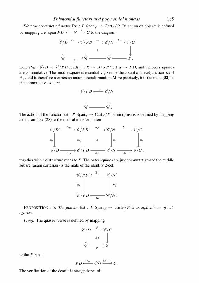
Polynomial functors and polynomial monads 185
We now construct a functor Ext : P-SpanC → CartC /P . Its action on objects is defined
by mapping a P-span P Dd←− N
c−→ C to the diagram
C /DP/D
��
��
C /P D
⇓��
�d �� C /N�c ��
��
C /C
��
CP
�� C C C .
Here P/D : C /D → C /P D sends f : X → D to P f : P X → P D, and the outer squaresare commutative. The middle square is essentially given by the counit of the adjunction �d ��d , and is therefore a cartesian natural transformation. More precisely, it is the mate [32] ofthe commutative square
C /P D
��
C /N�d��
��
C C .
The action of the functor Ext : P-SpanC → CartC /P on morphisms is defined by mappinga diagram like (28) to the natural transformation
C /D′
� f
��
P/D′�� C /P D′
⇓�P f
��
�d′�� C /N ′
�g
��
�c′ �� C /C ′
�h
��
C /DP/D
�� C /P D�d
�� C /N�c
�� C /C ,
together with the structure maps to P . The outer squares are just commutative and the middlesquare (again cartesian) is the mate of the identity 2-cell
C /P D′
�P f
��
C /N ′�d′��
�g
��
C /P D C /N .�d
��
PROPOSITION 5·6. The functor Ext : P-SpanC → CartC /P is an equivalence of cat-egories.
Proof. The quasi-inverse is defined by mapping
C /DQ
��
��
⇓ φ
C /C
��
CP
�� C
to the P-span
P D Q DφD��
Q(1D)�� C .
The verification of the details is straightforward.
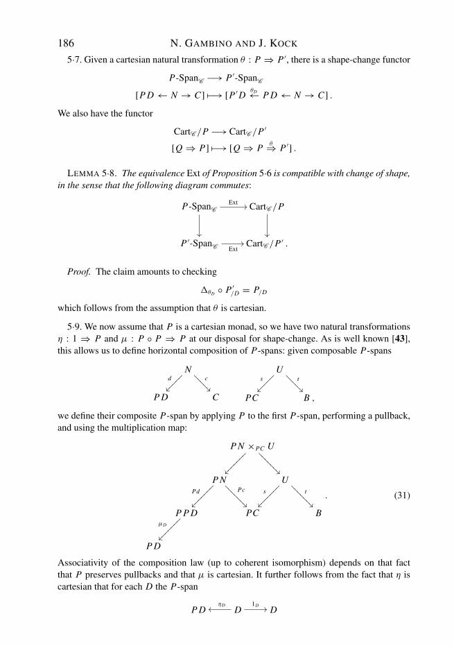
186 N. GAMBINO AND J. KOCK
5·7. Given a cartesian natural transformation θ : P ⇒ P ′, there is a shape-change functor
P-SpanC −→ P ′-SpanC
[P D ← N → C] �−→ [P ′ DθD← P D ← N → C] .
We also have the functor
CartC /P −→ CartC /P ′
[Q ⇒ P] �−→ [Q ⇒ Pθ⇒ P ′] .
LEMMA 5·8. The equivalence Ext of Proposition 5·6 is compatible with change of shape,in the sense that the following diagram commutes:
P-SpanCExt ��
��
CartC /P
��
P ′-SpanC Ext�� CartC /P ′ .
Proof. The claim amounts to checking
�θD ◦ P ′/D = P/D
which follows from the assumption that θ is cartesian.
5·9. We now assume that P is a cartesian monad, so we have two natural transformationsη : 1 ⇒ P and μ : P ◦ P ⇒ P at our disposal for shape-change. As is well known [43],this allows us to define horizontal composition of P-spans: given composable P-spans
Nc
����
���
d
������
�
CP D
Ut
����
���
s
������
�
B ,PC
we define their composite P-span by applying P to the first P-span, performing a pullback,and using the multiplication map:
P N ×PC U
����
����
�
������
���
P NPd
������
��� Pc
����
����
� Us
������
���
t
����
����
�
P P DμD
������
���
PC B
P D
. (31)
Associativity of the composition law (up to coherent isomorphism) depends on that factthat P preserves pullbacks and that μ is cartesian. It further follows from the fact that η iscartesian that for each D the P-span
P D DηD��
1D �� D

Polynomial functors and polynomial monads 187
is the identity P-spans for the composition law (up to coherent isomorphisms). It is clearthat these constructions are functorial in vertical maps between P-spans, yielding alto-gether a double category of P-spans, denoted P-SpanC : the objects and vertical morph-isms are those of C , the horizontal arrows are the P-spans, and the squares are diagramslike (28).
5·10. We also have a double-category structure on CartC /P: the horizontal composite ofQ ⇒ P with R ⇒ P is R ◦ Q ⇒ P ◦ P ⇒ P , and the horizontal identity arrow is Id ⇒ P .Let us verify that the extension of a horizontal composite is isomorphic to the composite ofthe extensions: in the diagram
C /CP/C
������
����
C /N
�c
����������
P/N ������
����
C /PC�s
������
����
C /P D
�d
����������
P/P D
������
����
C /P N
�(Pc)
����������
������
����
B.C. C /U�t
������
����
C /D
P/D
����������
(P P)/D
�� C /P P D
�(Pd)
����������C /P N ×PC U
����������C /B
the top path is the composite of the extension functors, and the bottom path is the extensionof the composite span. The square marked B.C. is the Beck-Chevalley isomorphism for thecartesian square (31), and the other squares, as well as the triangle, are clearly commutative.The following proposition now follows from Proposition 5·6.
PROPOSITION 5·11. The functor Ext : P-SpanC →CartC /P is an equivalence of doublecategories, in fact an equivalence of framed bicategories.
We just owe to make explicit how the double category of P-spans is a framed bicategory: toeach vertical map u : D′ → D we associate the P-span
P D′ ηD′←− D′ u−→ D .
This is a left adjoint; its right adjoint is the P-span
P DηD◦u←− D′ =−→ D′
as follows by noting that their extensions are respectively �u and �u . For this the importantfact is that η is cartesian. With this observation it is clear that the equivalence is framed.
5·12. We now specialise to the case of interest, where C = E /I and P is a polynomialmonad on E /I , represented by
I ←− B −→ A −→ I.

188 N. GAMBINO AND J. KOCK
Since now all the maps involved in the P-spans are over I , a P-span can be interpreted asa commutative diagram
Nd
������
� c
����
���
C
������
�P D
����
���
I .
If C is an object of C , i.e. a map in E with codomain I , we shall write C also for itsdomain, and we have a natural identification of slices C /C � E /C . That P : E /I →E /I is a polynomial monad, means thanks to Lemma 2·2, that all objects in CartE /I /P arepolynomial again, so CartE /I /P � Polyc
E /P , the category of polynomials cartesian over Pin the double-category sense. In conclusion:
PROPOSITION 5·13. The functor Ext : P-SpanE /I → PolycE /P is an equivalence of
framed bicategories.
5·14. It is a natural question whether there is a direct comparison between P-spans andpolynomials over P , without reference to their extensions. This is indeed the case, as wenow proceed to establish, exploiting the framed structure. Given a polynomial over P , like
Q : D
u
��
M��
��
��
�� N
��
�� C
��
P : I B�� �� A �� I .
Consider the canonical factorisation of this morphism through the source lift of P along u(cf. 3·11):
Q : D M�� ��
��
�� Nc ��
d
��
C
��
(u, Id)∗ P : D ·����
��
f�� P D ��
��
I
D
u
��
·��
��
��
P : I B�� �� A �� I .
(32)
Now we just read off the associated P-span:
Nc ��
d
��
C
��
P D �� I .
Conversely, given such a P-span, place it on top of the rightmost leg of P ◦ �α = (u, Id)∗ P(the middle row of the diagram, which depends only on α and P), and let M be the pullbackof N → P(D) along the arrow labelled f . It is easy to see that these constructions arefunctorial, yielding an equivalence of hom categories Polyc
E (D, C)/P � P-SpanE /I (D, C).
Polynomial functors and polynomial monads 189
Example 5·15. Endo-P-spans PC ← N → C , that is, polynomial endofunctors overP , are called C-coloured P-collections. If furthermore C = I we simply call them P-collections. These are just polynomial endofunctors Q : E /I → E /I equipped with acartesian natural transformation to P . This category is itself a slice of E : it is easy to seethat the functor
PolycE (I, I )/P −→ E /P1
Q �−→ [Q1 → P1]is an equivalence of categories.
5·16. Burroni [12], Leinster [43] and Hermida [22] define P-multicategories (also calledcoloured P-operads) as monads in the bicategory of P-spans. P-multicategories are alsomonads in the double category of P-spans — this description also provides the P-multifunctors as (oplax) cartesian monad maps. P-multicategories based at the terminalobject in E /I are called P-operads. If the base monad P is a polynomial monad, the equival-ence of Proposition 5·13 induces an equivalence of the categories of monads, as summarisedin the corollary below.
In the classical example, E is Set and P is the free-monoid monad M of Example 1·9.In this case, M-multicategories are the classical multicategories of Lambek [40], which arealso called coloured nonsymmetric operads. In the one-object case, M-operads are the plain(nonsymmetric) operads. The other standard example is taking P to be the identity monadon Set. Then P-multicategories are just small categories and P-operads are just monoids.Hence small categories are essentially polynomial monads on some slice Set/C with anoplax cartesian double-categorical monad map to Id, and monoids are essentially polynomialmonads on Set with a cartesian monad map to Id. In summary, we have the following result.
COROLLARY 5·17. There are natural equivalences of categories
P-Multicat � PolyMnd/P P-Operad � PolyMnd(1)/P
Multicat � PolyMnd/M PlainOperad � PolyMnd(1)/M
Cat � PolyMnd/Id Monoid � PolyMnd(1)/Id .
5·18. The double category of polynomials is very convenient for reasoning with P-multicategories. The role of the base monad P for P-multicategories is to specify a profilefor the operations. This involves specifying the shape of the input data, and it may also in-volve type constraints on input and output. In the classical case of P = M , the fibres ofN
′ → N (Example 1·9) are finite ordinals, expressing the fact that inputs to an operation in aclassical multicategory must be given as a finite list of objects. In this case there are no typeconstraints imposed by P on the operations.
For a more complicated example, let P : Set/N → Set/N be the free-plain-operad monad,which takes a collection (i.e. an object in Set/N) and returns the free plain operad on it [43,p.135, p.145, p.155]. This monad is polynomial (cf. [36]): it is represented by
Ns←− Tr•
p−→ Trt−→ N ,
where Tr denotes the set of (isomorphism classes of) finite planar rooted trees, and Tr•
denotes the set of (isomorphism classes of) finite planar rooted trees with a marked node.The map s returns the number of input edges of the marked node; the map p forgets the

190 N. GAMBINO AND J. KOCK
mark, and t returns the number of leaves. A P-multicategory Q has a set of objects and a setof operations. Each operation has its input slots organised as the set of nodes of some planarrooted tree, since this is how the p-fibres look like. Furthermore, there are type constraints:each object of Q must be typed in N, via a number that we shall call the degree of theobject, and a compatibility is required between the typing of operations and the typing ofobjects. Namely, the degree of the output object of an operation must equal the total numberof leaves of the tree whose nodes index the input, and the degree of the object associated toa particular input slot must equal the number of incoming edges of the corresponding nodein the tree. All this is displayed with clarity by the fact that Q is given by a diagram
Q : D
α
��
M��
��
��
�� N
β
��
�� D
α
��
P : N Tr•�� �� Tr �� N.
The typing of the operations is concisely given by the map β, and the organisation of theinputs in terms of the fibres of the middle map of P is just the cartesian condition on themiddle square. The typing of objects is encoded by α and the compatibility conditions,somewhat tedious to formulate in prose, are nothing but commutativity of the outer squares.
Finite planar rooted trees can be seen as M-trees, where M : Set → Set is the free-monoidmonad (1·9). Abstract trees, in turn, can be seen as polynomial functors (1·10): to a tree isassociated the polynomial functor
A ←− N ′ −→ N −→ A,
where A is the set of edges, N is the set of nodes, and N ′ is the set of nodes with a markedincoming edge. Formally, an M-tree is a tree over M in Polyc
E , that is to say a diagram
A
��
N ′��
��
��
�� N
��
�� A
��
1 N′�� �� N �� 1 .
Acknowledgments. Both authors have had the privilege of being mentored by AndreJoyal, and have benefited a lot from his generous guidance. In particular, our view on poly-nomial functors has been shaped very much by his ideas, and the results of Section 2 weessentially learned from him. We also thank Anders Kock and Mark Weber for numeroushelpful discussions. Part of this work was carried out at the CRM in Barcelona during thespecial year on Homotopy Theory and Higher Categories; we are grateful to the CRM forexcellent working conditions and for support for the first-named author. The second-namedauthor acknowledges support from research grants MTM2006-11391 and MTM2007-63277of the Spanish Ministry for Science and Innovation.
REFERENCES
[1] M. ABBOTT. Categories of containers. Ph.D. thesis. University of Leicester (2003).[2] M. ABBOTT, T. ALTENKIRCH and N. GHANI. Categories of containers. Foundations of Software
Science and Computation Structures (A. D. Gordon, ed.). Lecture Notes in Computer Science, vol.2620 (Springer, 2003), pp. 23–38.
[3] M. ABBOTT, T. ALTENKIRCH and N. GHANI. Representing nested inductive types using W-types.Automata, languages and programming (J. Dıaz, J. Karhumaki, A. Lepisto, D. Sannella, eds.) Lec-ture Notes in Computer Science, vol. 3142. (Springer, Berlin, 2004), pp. 59–71.

Polynomial functors and polynomial monads 191[4] M. ABBOTT, T. ALTENKIRCH and N. GHANI. Containers: constructing strictly positive types. The-
oret. Comput. Sci. 342 (2005), pp. 3–27.[5] T. ALTENKIRCH and P. MORRIS. Indexed containers. Proceedings of the 24th IEEE Symposium in
Logic in Computer Science (LICS 2009), IEEE Computer Society, 2009.[6] J. C. BAEZ and J. DOLAN. Higher-dimensional algebra III. n-categories and the algebra of opetopes.
Adv. Math. 135 (1998), pp. 145–206.[7] M. BARR and C. WELLS. Toposes Triples and Theories (Springer-Verlag, 1983). Reprinted in Repr.
Theory Appl. Categ. 12 (2005), x+288 pp. (electronic).[8] J. BENABOU. Introduction to bicategories. Reports of the Midwest Category Theory Seminar
(J. Benabou et al., eds.) Lecture Notes in Math., vol. 47 (Springer-Verlag, 1967), pp. 1–77.[9] F. BERGERON, G. LABELLE and P. LEROUX. Combinatorial Species and Tree-Like Structures (Cam-
bridge University Press, 1998).[10] T. BISSON and A. JOYAL. The Dyer-Lashof algebra in bordism. C. R. Math. Rep. Acad. Sci. Canada
17 (1995), pp. 135–140.[11] M. BRUN. Witt vectors and Tambara functors. Adv. Math. 193 (2005), pp. 233–256.[12] A. BURRONI. T-categories (categories dans une triple). Cah. Topol. Geom. Differ. Categ. 12 (1971),
pp. 215–315.[13] A. CARBONI and P. JOHNSTONE. Connected limits, familial representability and Artin glueing. Math.
Structures Comput. Sci. 5 (1995), 441–459, with Corrigenda in Math. Structures Comput. Sci. 14(2004), pp. 185–187.
[14] Y. DIERS. Categories localisables. Ph.D. thesis. Universite de Paris VI (1977).[15] P. CLAIRAMBAULT and P. DYBJER. The biequivalence of locally Cartesian closed categories and
Martin-Lof type theories. Typed lambda calculi and applications. Lecture Notes in Computer Sci-ence, vol. 6690. (Springer, 2011), pp. 91–106.
[16] P. FREYD. Aspects of topoi. Bull. Austral. Math. Soc. 7 (1972), pp. 1–76 and pp. 467–480.[17] N. GAMBINO and M. HYLAND. Wellfounded trees and dependent polynomial functors. Types for
proofs and programs (S. Berardi, M. Coppo, and F. Damiani, eds.), Lecture Notes in ComputerScience, vol. 3085, (Springer, 2004), pp. 210–225.
[18] J.-Y. GIRARD. Normal functors, power series and λ-calculus. Ann. Pure Appl. Logic 37 (1988),pp. 129–177.
[19] M. GRANDIS and R. PARE. Adjoints for double categories. Addenda to “Limits in double categories”.Cah. Topol. Geom. Differ. Categ. 45 (2004), pp. 193–240.
[20] A. GROTHENDIECK. Revetements etales et groupe fondamental (SGA1). Lecture Notes in Mathem-atics, vol. 224 (Springer, 1971).
[21] P. HANCOCK and A. SETZER. Interactive programs and weakly final coalgebras in dependent typetheory. From sets and types to topology and analysis, Oxford Logic Guides, vol. 48. (Oxford Uni-versity Press, 2005), pp. 115–136.
[22] C. HERMIDA. Representable multicategories. Adv. Math. 151 (2000), pp. 164–225.[23] M. HOFMANN. On the interpretation of type theory in locally Cartesian closed categories. Computer
Science Logic (Kasimierz 1994). Lecture Notes in Computer Science, vol. 933 (Springer, 1995),pp. 427–441.
[24] P. HYVERNAT. A logical investigation of interaction systems. Ph.D. thesis. Chalmers University(2005).
[25] C. B. JAY. A semantics for shape. Sci. Comput. Programming 25 (1995), pp. 251–283.[26] C. B. JAY and J. R. B. COCKETT. Shapely types and shape polymorphism, Programming languages
and systems - ESOP ’94 (D. Sannella, ed.) Lecture Notes in Computer Science, vol. 788 (Springer,1994), pp. 302–316.
[27] P. JOHNSTONE. Cartesian monads on toposes. J. Pure Appl. Alg. 116 (1997), pp. 199–220.[28] A. JOYAL. Une theorie combinatoire des series formelles. Adv. Math. 42 (1981), pp. 1–82.[29] A. JOYAL. Foncteurs analytiques et especes de structures. Combinatoire Enumerative
(Montreal/Quebec, 1985), Lecture Notes in Math. vol. 1234 (Springer, 1986), pp. 126–159.[30] G. M. KELLY. A unified treatment of transfinite constructions for free algebras, free monoids, colim-
its, associated sheaves and so on. Bull. Austral. Math. Soc. 22 (1980), pp. 1–83.[31] G. M. KELLY. Basic concepts of enriched category theory. London Mathematical Society Lecture
Note Series, vol. 64 (Cambridge University Press, 1982), Reprinted in Repr. Theory Appl. Categ.10 (2005), vi+137 pp. (electronic).
[32] G. M. KELLY and R. H. STREET. Review of the elements of 2-categories, Category Seminar (Sydney1972/1973) (G. M. Kelly, ed.). Lecture Notes in Mathematics, vol. 420 (Springer-Verlag, Berlin,1974), pp. 75–103.
[33] A. KOCK. Strong functors and monoidal monads. Arch. Math. (Basel) 23 (1972), pp. 113–120.

192 N. GAMBINO AND J. KOCK
[34] A. KOCK and J. KOCK. Local fibered right adjoints are polynomial. arXiv:1005.4236, 2010, to appearin Math. Struct. Comp. Sci.
[35] J. KOCK. Polynomial functors and trees. Internat. Math. Res. Not. 2011 (2011) pp. 609–673.[36] J. KOCK, A. JOYAL, M. BATANIN and J.-F. MASCARI. Polynomial functors and opetopes. Adv.
Math. 224 (2010), pp. 2690–2737.[37] M. KONTSEVICH and Y. SOIBELMAN. Deformations of algebras over operads and the Deligne con-
jecture. Conference Moshe Flato 1999, Vol. I (Dijon) Math. Phys. Stud. vol. 21, (Kluwer AcademicPublishers, 2000), pp. 255–307.
[38] S. LACK and R. STREET. The formal theory of monads. II. J. Pure Appl. Alg. 175 (2002), pp. 243–265.
[39] F. LAMARCHE. Modelling polymorphism with categories. Ph.D. thesis. McGill University (1988).[40] J. LAMBEK. Deductive systems and categories. II. Standard constructions and closed categories. Cat-
egory Theory, Homology Theory and their Applications, I (Battelle Institute Conference, Seattle,Wash. 1968, Vol. One) (Springer, Berlin, 1969), pp. 76–122.
[41] S. MAC LANE and I. MOERDIJK. Sheaves in Geometry and Logic: a First Introduction to ToposTheory (Springer, New York, 1992).
[42] T. LEINSTER. A survey of definitions of n-category. Theory Appl. Categ. 10 (2002), pp. 1–70 (elec-tronic).
[43] T. LEINSTER. Higher operads, higher categories. London Mathematical Society Lecture Note Series,vol. 298 (Cambridge University Press, 2004).
[44] I. G. MACDONALD. Symmetric functions and Hall polynomials. Oxford Mathematical Monographs(The Clarendon Press Oxford University Press, New York, 1979).
[45] M. MAKKAI and G. REYES. First-order categorical logic. Lecture Notes in Mathematics, vol. 611(Springer-Verlag, Berlin, 1977).
[46] E. G. MANES and M. A. ARBIB. Algebraic Approaches to Program Semantics (Springer-Verlag,New York, 1986).
[47] N. MARTINS–FERREIRA. Pseudo-categories. J. Homotopy Relat. Struct. 1 (2006), pp. 47–78.[48] I. MOERDIJK and E. PALMGREN. Wellfounded trees in categories. Ann. Pure Appl. Logic 104 (2000),
pp. 189–218.[49] E. MOGGI, G. BELLE and C. B. JAY. Monads, shapely functors and transversals. Electron. Notes
Theor. Comput. Sci. 29 (1999), pp. 187–208.[50] B. NORDSTROM, K. PETERSSON and J. M. SMITH. Programming in Martin-Lof Type Theory: an
Introduction (Oxford University Press, 1990).[51] B. NORDSTROM, K. PETERSSON and J. M. SMITH. Martin-Lof Type Theory. Handbook of Logic in
Computer Science. Volume V (S. Abramsky, D. M. Gabbay, and T. S. E. Maibaum, eds.) (OxfordUniversity Press, 2001, pp. 1–37).
[52] K. PETERSSON and D. SYNEK. A set constructor for inductive sets in Martin-Lof type theory. Cat-egory Theory and Computer Science (Manchester 1989) (D. E. Rydeheard, P. Dybjer, A. M. Pitts,and A. Poigne, eds.). Lecture Notes in Computer Science, vol. 389 (Springer, 1989, pp. 128–140).
[53] T. PIRASHVILI. Polynomial functors over finite fields (after Franjou, Friedlander, Henn,Lannes, Schwartz, Suslin). Seminaire Bourbaki, Vol. 1999/2000. Asterisque, vol. 276 (SocieteMathematique de France, 2002), pp. 369–388.
[54] R. A. G. SEELY. Locally cartesian closed categories and type theory. Math. Proc. Camb. Phil. Soc.95 (1984), pp. 33–48.
[55] M. SHULMAN. Framed bicategories and monoidal fibrations. Theory Appl. Categ. 20 (2008), pp. 650–738 (electronic).
[56] R. STREET. The formal theory of monads. J. Pure Appl. Alg. 2 (1972), pp. 149–169.[57] R. STREET. The petit topos of globular sets. J. Pure Appl. Alg. 154 (2000), pp. 299–315.[58] N. STRICKLAND. Tambara functors. arXiv:1205.2516, 2012.[59] D. TAMBARA. On multiplicative transfer. Comm. Alg. 21 (1993), pp. 1393–1420.[60] P. TAYLOR. Quantitative domains, groupoids and linear logic. Category theory and computer science
(D. H. Pitt, D. E. Rydeheard, P. Dybjer, A. M. Pitts, and A. Poigne, eds.) Lecture Notes in ComputerScience, vol. 389 (Springer, Berlin, 1989), pp. 155–181.
[61] M. WEBER. Generic morphisms, parametric representations and weakly Cartesian monads. TheoryAppl. Categ. 13 (2004), pp. 191–234 (electronic).
[62] M. WEBER. Familial 2-functors and parametric right adjoints. Theory Appl. Categ. 18 (2007),pp. 665–732 (electronic).
[63] M. WEBER. Polynomials in categories with pullbacks. arXiv:1106.1983, 2011.[64] M. ZAWADOWSKI. Lax monoidal fibrations. Models, logics and higher-dimensional categories.
(American Mathematical Society, 2011), pp. 341–426.