2

SINGLE PARTICLE MOTION

2.1 INTRODUCTION

This chapter will briefly review the issues and problems involved in con-structing the equations of motion for individual particles, drops or bubblesmoving through a fluid. For convenience we shall use the generic name par-ticle to refer to the finite pieces of the disperse phase or component. Theanalyses are implicitly confined to those circumstances in which the interac-tions between neighboring particles are negligible. In very dilute multiphaseflows in which the particles are very small compared with the global dimen-sions of the flow and are very far apart compared with the particle size, itis often sufficient to solve for the velocity and pressure, ui(xi, t) and p(xi, t),of the continuous suspending fluid while ignoring the particles or dispersephase. Given this solution one could then solve an equation of motion forthe particle to determine its trajectory. This chapter will focus on the con-struction of such a particle or bubble equation of motion.

The body of fluid mechanical literature on the subject of flows aroundparticles or bodies is very large indeed. Here we present a summary thatfocuses on a spherical particle of radius, R, and employs the following com-mon notation. The components of the translational velocity of the centerof the particle will be denoted by Vi(t). The velocity that the fluid wouldhave had at the location of the particle center in the absence of the particlewill be denoted by Ui(t). Note that such a concept is difficult to extend tothe case of interactive multiphase flows. Finally, the velocity of the particlerelative to the fluid is denoted by Wi(t) = Vi − Ui.

Frequently the approach used to construct equations for Vi(t) (or Wi(t))given Ui(xi, t) is to individually estimate all the fluid forces acting on theparticle and to equate the total fluid force, Fi, to mpdVi/dt (where mp isthe particle mass, assumed constant). These fluid forces may include forces

52

due to buoyancy, added mass, drag, etc. In the absence of fluid acceleration(dUi/dt = 0) such an approach can be made unambiguously; however, inthe presence of fluid acceleration, this kind of heuristic approach can bemisleading. Hence we concentrate in the next few sections on a fundamentalfluid mechanical approach, that minimizes possible ambiguities. The classicalresults for a spherical particle or bubble are reviewed first. The analysis isconfined to a suspending fluid that is incompressible and Newtonian so thatthe basic equations to be solved are the continuity equation

∂uj

∂xj= 0 (2.1)

and the Navier-Stokes equations

ρC

{∂ui

∂t+ uj

∂ui

∂xj

}= − ∂p

∂xi+ ρCνC

∂2ui

∂xj∂xj(2.2)

where ρC and νC are the density and kinematic viscosity of the suspendingfluid. It is assumed that the only external force is that due to gravity, g.Then the actual pressure is p′ = p− ρCgz where z is a coordinate measuredvertically upward.

Furthermore, in order to maintain clarity we confine our attention torectilinear relative motion in a direction conveniently chosen to be the x1

direction.

2.2 FLOWS AROUND A SPHERE

2.2.1 At high Reynolds number

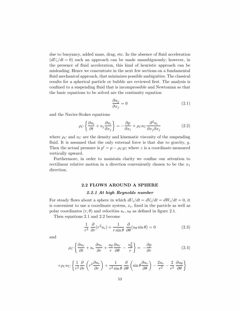
For steady flows about a sphere in which dUi/dt = dVi/dt = dWi/dt = 0, itis convenient to use a coordinate system, xi, fixed in the particle as well aspolar coordinates (r, θ) and velocities ur, uθ as defined in figure 2.1.

Then equations 2.1 and 2.2 become

1r2

∂

∂r(r2ur) +

1r sin θ

∂

∂θ(uθ sin θ) = 0 (2.3)

and

ρC

{∂ur

∂t+ ur

∂ur

∂r+uθ

r

∂ur

∂θ− u2

θ

r

}= −∂p

∂r(2.4)

+ρCνC

{1r2

∂

∂r

(r2∂ur

∂r

)+

1r2 sin θ

∂

∂θ

(sin θ

∂ur

∂θ

)− 2ur

r2− 2r2

∂uθ

∂θ

}

53

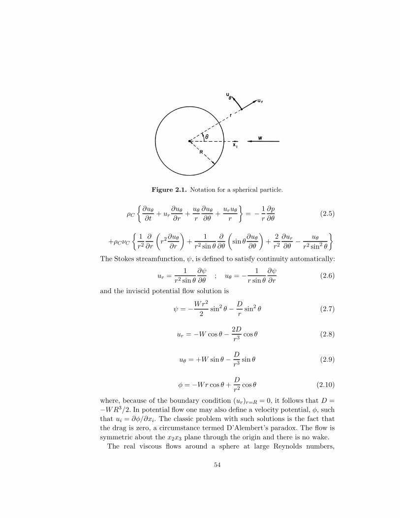
Figure 2.1. Notation for a spherical particle.

ρC

{∂uθ

∂t+ ur

∂uθ

∂r+uθ

r

∂uθ

∂θ+uruθ

r

}= − 1

r

∂p

∂θ(2.5)

+ρCνC

{1r2

∂

∂r

(r2∂uθ

∂r

)+

1r2 sin θ

∂

∂θ

(sin θ

∂uθ

∂θ

)+

2r2∂ur

∂θ− uθ

r2 sin2 θ

}

The Stokes streamfunction, ψ, is defined to satisfy continuity automatically:

ur =1

r2 sin θ∂ψ

∂θ; uθ = − 1

r sin θ∂ψ

∂r(2.6)

and the inviscid potential flow solution is

ψ = −Wr2

2sin2 θ − D

rsin2 θ (2.7)

ur = −W cos θ − 2Dr3

cos θ (2.8)

uθ = +W sin θ − D

r3sin θ (2.9)

φ = −Wr cos θ +D

r2cos θ (2.10)

where, because of the boundary condition (ur)r=R = 0, it follows that D =−WR3/2. In potential flow one may also define a velocity potential, φ, suchthat ui = ∂φ/∂xi. The classic problem with such solutions is the fact thatthe drag is zero, a circumstance termed D’Alembert’s paradox. The flow issymmetric about the x2x3 plane through the origin and there is no wake.

The real viscous flows around a sphere at large Reynolds numbers,

54

Figure 2.2. Smoke visualization of the nominally steady flows (fromleft to right) past a sphere showing, at the top, laminar separation atRe = 2.8 × 105 and, on the bottom, turbulent separation atRe = 3.9 × 105.Photographs by F.N.M.Brown, reproduced with the permission of the Uni-versity of Notre Dame.

Re = 2WR/νC > 1, are well documented. In the range from about 103 to3 × 105, laminar boundary layer separation occurs at θ ∼= 84◦ and a largewake is formed behind the sphere (see figure 2.2). Close to the sphere thenear-wake is laminar; further downstream transition and turbulence occur-ring in the shear layers spreads to generate a turbulent far-wake. As theReynolds number increases the shear layer transition moves forward until,quite abruptly, the turbulent shear layer reattaches to the body, resultingin a major change in the final position of separation (θ ∼= 120◦) and in theform of the turbulent wake (figure 2.2). Associated with this change in flow

55

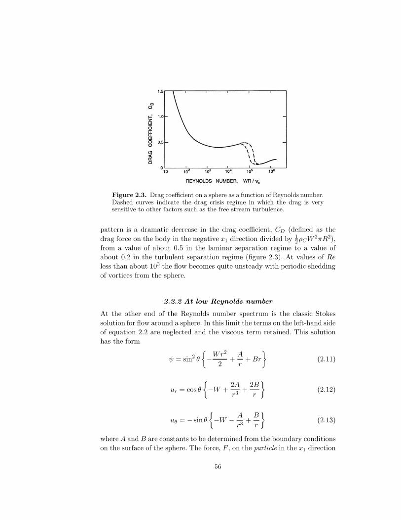
Figure 2.3. Drag coefficient on a sphere as a function of Reynolds number.Dashed curves indicate the drag crisis regime in which the drag is verysensitive to other factors such as the free stream turbulence.

pattern is a dramatic decrease in the drag coefficient, CD (defined as thedrag force on the body in the negative x1 direction divided by 1

2ρCW2πR2),

from a value of about 0.5 in the laminar separation regime to a value ofabout 0.2 in the turbulent separation regime (figure 2.3). At values of Reless than about 103 the flow becomes quite unsteady with periodic sheddingof vortices from the sphere.

2.2.2 At low Reynolds number

At the other end of the Reynolds number spectrum is the classic Stokessolution for flow around a sphere. In this limit the terms on the left-hand sideof equation 2.2 are neglected and the viscous term retained. This solutionhas the form

ψ = sin2 θ

{−Wr2

2+A

r+ Br

}(2.11)

ur = cos θ{−W +

2Ar3

+2Br

}(2.12)

uθ = − sin θ{−W − A

r3+B

r

}(2.13)

where A and B are constants to be determined from the boundary conditionson the surface of the sphere. The force, F , on the particle in the x1 direction

56

is

F1 =43πR2ρCνC

{−4WR

+8AR4

+2BR2

}(2.14)

Several subcases of this solution are of interest in the present context. Thefirst is the classic Stokes (1851) solution for a solid sphere in which the no-slipboundary condition, (uθ)r=R = 0, is applied (in addition to the kinematiccondition (ur)r=R = 0). This set of boundary conditions, referred to as theStokes boundary conditions, leads to

A = −WR3

4, B = +

3WR

4and F1 = −6πρCνCWR (2.15)

The second case originates with Hadamard (1911) and Rybczynski (1911)who suggested that, in the case of a bubble, a condition of zero shear stresson the sphere surface would be more appropriate than a condition of zerotangential velocity, uθ. Then it transpires that

A = 0 , B = +WR

2and F1 = −4πρCνCWR (2.16)

Real bubbles may conform to either the Stokes or Hadamard-Rybczynskisolutions depending on the degree of contamination of the bubble surface,as we shall discuss in more detail in section 3.3. Finally, it is of interest toobserve that the potential flow solution given in equations 2.7 to 2.10 is alsoa subcase with

A = +WR3

2, B = 0 and F1 = 0 (2.17)

However, another paradox, known as the Whitehead paradox, arises whenthe validity of these Stokes flow solutions at small (rather than zero)Reynolds numbers is considered. The nature of this paradox can be demon-strated by examining the magnitude of the neglected term, uj∂ui/∂xj, inthe Navier-Stokes equations relative to the magnitude of the retained termνC∂

2ui/∂xj∂xj. As is evident from equation 2.11, far from the sphere theformer is proportional toW 2R/r2 whereas the latter behaves like νCWR/r3.It follows that although the retained term will dominate close to the body(provided the Reynolds number Re = 2WR/νC � 1), there will always be aradial position, rc, given by R/rc = Re beyond which the neglected term willexceed the retained viscous term. Hence, even if Re� 1, the Stokes solutionis not uniformly valid. Recognizing this limitation, Oseen (1910) attemptedto correct the Stokes solution by retaining in the basic equation an approxi-mation to uj∂ui/∂xj that would be valid in the far field, −W∂ui/∂x1. Thus

57

the Navier-Stokes equations are approximated by

−W ∂ui

∂x1= − 1

ρC

∂p

∂xi+ νC

∂2ui

∂xj∂xj(2.18)

Oseen was able to find a closed form solution to this equation that satisfiesthe Stokes boundary conditions approximately:

ψ = −WR2

{r2 sin2 θ

2R2+R sin2 θ

4r+

3νC(1 + cos θ)2WR

(1 − e

W r2νC (1−cos θ)

)}(2.19)

which yields a drag force

F1 = −6πρCνCWR

{1 +

316

Re

}(2.20)

It is readily shown that equation 2.19 reduces to equation 2.11 as Re→ 0.The corresponding solution for the Hadamard-Rybczynski boundary con-ditions is not known to the author; its validity would be more question-able since, unlike the case of Stokes boundary conditions, the inertial termsuj∂ui/∂xj are not identically zero on the surface of the bubble.

Proudman and Pearson (1957) and Kaplun and Lagerstrom (1957) showedthat Oseen’s solution is, in fact, the first term obtained when the methodof matched asymptotic expansions is used in an attempt to patch togetherconsistent asymptotic solutions of the full Navier-Stokes equations for boththe near field close to the sphere and the far field. They also obtained thenext term in the expression for the drag force.

F1 = −6πρCνCWR

{1 +

316Re+

9160

Re2ln

(Re

2

)+ 0(Re2)

}(2.21)

The additional term leads to an error of 1% at Re = 0.3 and does not,therefore, have much practical consequence.

The most notable feature of the Oseen solution is that the geometry ofthe streamlines depends on the Reynolds number. The downstream flow isnot a mirror image of the upstream flow as in the Stokes or potential flowsolutions. Indeed, closer examination of the Oseen solution reveals that,downstream of the sphere, the streamlines are further apart and the flowis slower than in the equivalent upstream location. Furthermore, this effectincreases with Reynolds number. These features of the Oseen solution areentirely consistent with experimental observations and represent the initialdevelopment of a wake behind the body.

The flow past a sphere at Reynolds numbers between about 0.5 and severalthousand has proven intractable to analytical methods though numerical so-

58

lutions are numerous. Experimentally, it is found that a recirculating zone(or vortex ring) develops close to the rear stagnation point at about Re = 30(see Taneda 1956 and figure 2.4). With further increase in the Reynoldsnumber this recirculating zone or wake expands. Defining locations on thesurface by the angle from the front stagnation point, the separation pointmoves forward from about 130◦ at Re = 100 to about 115◦ at Re = 300. Inthe process the wake reaches a diameter comparable to that of the spherewhen Re ≈ 130. At this point the flow becomes unstable and the ring vor-tex that makes up the wake begins to oscillate (Taneda 1956). However, itcontinues to be attached to the sphere until about Re = 500 (Torobin andGauvin 1959).

At Reynolds numbers above about 500, vortices begin to be shed andthen convected downstream. The frequency of vortex shedding has not beenstudied as extensively as in the case of a circular cylinder and seems to varymore with Reynolds number. In terms of the conventional Strouhal number,Str, defined as

Str = 2fR/W (2.22)

the vortex shedding frequencies, f , that Moller (1938) observed correspondto a range of Str varying from 0.3 at Re = 1000 to about 1.8 at Re = 5000.Furthermore, as Re increases above 500 the flow develops a fairly steadynear-wake behind which vortex shedding forms an unsteady and increasinglyturbulent far-wake. This process continues until, at a value of Re of the orderof 1000, the flow around the sphere and in the near-wake again becomesquite steady. A recognizable boundary layer has developed on the front ofthe sphere and separation settles down to a position about 84◦ from thefront stagnation point. Transition to turbulence occurs on the free shearlayer (which defines the boundary of the near-wake) and moves progressivelyforward as the Reynolds number increases. The flow is similar to that of thetop picture in figure 2.2. Then the events described in the previous sectionoccur with further increase in the Reynolds number.

Since the Reynolds number range between 0.5 and several hundred canoften pertain in multiphase flows, one must resort to an empirical formulafor the drag force in this regime. A number of empirical results are available;for example, Klyachko (1934) recommends

F1 = −6πρCνCWR

{1 +

Re23

6

}(2.23)

which fits the data fairly well up to Re ≈ 1000. At Re = 1 the factor in the

59

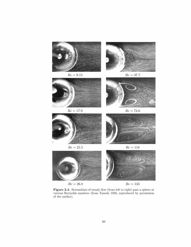
Re = 9.15 Re = 37.7

Re = 17.9 Re = 73.6

Re = 25.5 Re = 118

Re = 26.8 Re = 133

Figure 2.4. Streamlines of steady flow (from left to right) past a sphere atvarious Reynolds numbers (from Taneda 1956, reproduced by permissionof the author).

60

square brackets is 1.167, whereas the same factor in equation 2.20 is 1.187.On the other hand, at Re = 1000, the two factors are respectively 17.7 and188.5.

2.2.3 Molecular effects

When the mean free path of the molecules in the surrounding fluid, λ, be-comes comparable with the size of the particles, the flow will clearly deviatefrom the continuum models, that are only relevant when λ� R. The Knud-sen number, Kn = λ/2R, is used to characterize these circumstances, andCunningham (1910) showed that the first-order correction for small but finiteKnudsen number leads to an additional factor, (1 + 2AKn), in the Stokesdrag for a spherical particle. The numerical factor, A, is roughly a constantof order unity (see, for example, Green and Lane 1964).

When the impulse generated by the collision of a single fluid moleculewith the particle is large enough to cause significant change in the particlevelocity, the resulting random motions of the particle are called Brownianmotion (Einstein 1956). This leads to diffusion of solid particles suspendedin a fluid. Einstein showed that the diffusivity, D, of this process is given by

D = kT/6πμCR (2.24)

where k is Boltzmann’s constant. It follows that the typical rms displace-ment of the particle in a time, t, is given by (kT t/3πμCR)

12 . Brownian

motion is usually only significant for micron- and sub-micron-sized parti-cles. The example quoted by Einstein is that of a 1 μm diameter particlein water at 17◦C for which the typical displacement during one second is0.8 μm.

A third, related phenomenon is the response of a particle to the collisionsof molecules when there is a significant temperature gradient in the fluid.Then the impulses imparted to the particle by molecular collisions on thehot side of the particle will be larger than the impulses on the cold side. Theparticle will therefore experience a net force driving it in the direction of thecolder fluid. This phenomenon is known as thermophoresis (see, for example,Davies 1966). A similar phenomenon known as photophoresis occurs whena particle is subjected to nonuniform radiation. One could include in thislist the Bjerknes forces described in the section 3.4 since they constitutesonophoresis, namely forces acting on a particle in a sound field.

61

2.3 UNSTEADY EFFECTS

2.3.1 Unsteady particle motions

Having reviewed the steady motion of a particle relative to a fluid, we mustnow consider the consequences of unsteady relative motion in which eitherthe particle or the fluid or both are accelerating. The complexities of fluidacceleration are delayed until the next section. First we shall consider thesimpler circumstance in which the fluid is either at rest or has a steadyuniform streaming motion (U = constant) far from the particle. Clearly thesecond case is readily reduced to the first by a simple Galilean transformationand it will be assumed that this has been accomplished.

In the ideal case of unsteady inviscid potential flow, it can then be shownby using the concept of the total kinetic energy of the fluid that the forceon a rigid particle in an incompressible flow is given by Fi, where

Fi = −MijdVj

dt(2.25)

where Mij is called the added mass matrix (or tensor) though the nameinduced inertia tensor used by Batchelor (1967) is, perhaps, more descrip-tive. The reader is referred to Sarpkaya and Isaacson (1981), Yih (1969), orBatchelor (1967) for detailed descriptions of such analyses. The above men-tioned methods also show that Mij for any finite particle can be obtainedfrom knowledge of several steady potential flows. In fact,

Mij =ρC

2

∫volume

of fluid

uikujk d(volume) (2.26)

where the integration is performed over the entire volume of the fluid. Thevelocity field, uij, is the fluid velocity in the i direction caused by the steadytranslation of the particle with unit velocity in the j direction. Note thatthis means that Mij is necessarily a symmetric matrix. Furthermore, it isclear that particles with planes of symmetry will not experience a forceperpendicular to that plane when the direction of acceleration is parallel tothat plane. Hence if there is a plane of symmetry perpendicular to the kdirection, then for i �= k, Mki = Mik = 0, and the only off-diagonal matrixelements that can be nonzero are Mij, j �= k, i �= k. In the special case ofthe sphere all the off-diagonal terms will be zero.

Tables of some available values of the diagonal components of Mij aregiven by Sarpkaya and Isaacson (1981) who also summarize the experi-mental results, particularly for planar flows past cylinders. Other compila-tions of added mass results can be found in Kennard (1967), Patton (1965),

62

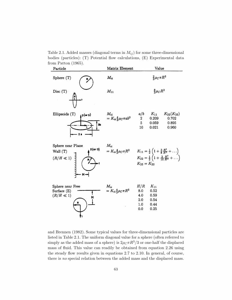
Table 2.1. Added masses (diagonal terms inMij) for some three-dimensionalbodies (particles): (T) Potential flow calculations, (E) Experimental datafrom Patton (1965).

and Brennen (1982). Some typical values for three-dimensional particles arelisted in Table 2.1. The uniform diagonal value for a sphere (often referred tosimply as the added mass of a sphere) is 2ρCπR

3/3 or one-half the displacedmass of fluid. This value can readily be obtained from equation 2.26 usingthe steady flow results given in equations 2.7 to 2.10. In general, of course,there is no special relation between the added mass and the displaced mass.

63

Consider, for example, the case of the infinitely thin plate or disc with zerodisplaced mass which has a finite added mass in the direction normal to thesurface. Finally, it should be noted that the literature contains little, if any,information on off-diagonal components of added mass matrices.

Now consider the application of these potential flow results to real viscousflows at high Reynolds numbers (the case of low Reynolds number flows willbe discussed in section 2.3.4). Significant doubts about the applicability ofthe added masses calculated from potential flow analysis would be justifiedbecause of the experience of D’Alembert’s paradox for steady potential flowsand the substantial difference between the streamlines of the potential andactual flows. Furthermore, analyses of experimental results will require theseparation of the added mass forces from the viscous drag forces. Usuallythis is accomplished by heuristic summation of the two forces so that

Fi = −MijdVj

dt− 1

2ρCACij|Vj|Vj (2.27)

where Cij is a lift and drag coefficient matrix and A is a typical cross-sectional area for the body. This is known as Morison’s equation (see Morisonet al. 1950).

Actual unsteady high Reynolds number flows are more complicated andnot necessarily compatible with such simple superposition. This is reflectedin the fact that the coefficients, Mij and Cij , appear from the experimentalresults to be not only functions of Re but also functions of the reducedtime or frequency of the unsteady motion. Typically experiments involveeither oscillation of a body in a fluid or acceleration from rest. The mostextensively studied case involves planar flow past a cylinder (for example,Keulegan and Carpenter 1958), and a detailed review of this data is includedin Sarpkaya and Isaacson (1981). For oscillatory motion of the cylinder withvelocity amplitude, UM , and period, t∗, the coefficients are functions of boththe Reynolds number, Re = 2UMR/νC , and the reduced period or Keulegan-Carpenter number, Kc = UM t∗/2R. When the amplitude, UM t

∗, is less thanabout 10R (Kc < 5), the inertial effects dominate and Mii is only a little lessthan its potential flow value over a wide range of Reynolds numbers (104 <

Re < 106). However, for larger values ofKc, Mii can be substantially smallerthan this and, in some range of Re and Kc, may actually be negative. Thevalues of Cii (the drag coefficient) that are deduced from experiments arealso a complicated function of Re and Kc. The behavior of the coefficientsis particularly pathological when the reduced period, Kc, is close to that ofvortex shedding (Kc of the order of 10). Large transverse or lift forces can begenerated under these circumstances. To the author’s knowledge, detailed

64

investigations of this kind have not been made for a spherical body, but onemight expect the same qualitative phenomena to occur.

2.3.2 Effect of concentration on added mass

Though most multiphase flow effects are delayed until later chapters it isconvenient at this point to address the issue of the effect on the added massof the particles in the surrounding mixture. It is to be expected that theadded mass coefficient for an individual particle would depend on the voidfraction of the surrounding medium. Zuber (1964) first addressed this issueusing a cell method and found that the added mass,Mii, for spherical bubblesincreased with volume fraction, α, like

Mii(α)Mii(0)

=(1 + 2α)(1 − α)

= 1 + 3α+ O(α2) (2.28)

The simplistic geometry assumed in the cell method (a concentric spheri-cal shell of fluid surrounding each spherical particle) caused later researchersto attempt improvements to Zuber’s analysis; for example, van Wijngaarden(1976) used an improved geometry (and the assumption of potential flow)to study the O(α) term and found that

Mii(α)Mii(0)

= 1 + 2.76α+ O(α2) (2.29)

which is close to Zuber’s result. However, even more accurate and morerecent analyses by Sangani et al. (1991) have shown that Zuber’s originalresult is, in fact, remarkably accurate even up to volume fractions as largeas 50% (see also Zhang and Prosperetti 1994).

2.3.3 Unsteady potential flow

In general, a particle moving in any flow other than a steady uniform streamwill experience fluid accelerations, and it is therefore necessary to considerthe structure of the equation governing the particle motion under thesecircumstances. Of course, this will include the special case of acceleration ofa particle in a fluid at rest (or with a steady streaming motion). As in theearlier sections we shall confine the detailed solutions to those for a sphericalparticle or bubble. Furthermore, we consider only those circumstances inwhich both the particle and fluid acceleration are in one direction, chosenfor convenience to be the x1 direction. The effect of an external force field

65

such as gravity will be omitted; it can readily be inserted into any of thesolutions that follow by the addition of the conventional buoyancy force.

All the solutions discussed are obtained in an accelerating frame of refer-ence fixed in the center of the fluid particle. Therefore, if the velocity of theparticle in some original, noninertial coordinate system, x∗i , was V (t) in thex∗1 direction, the Navier-Stokes equations in the new frame, xi, fixed in theparticle center are

∂ui

∂t+ uj

∂ui

∂xj= − 1

ρC

∂P

∂xi+ νC

∂2ui

∂xj∂xj(2.30)

where the pseudo-pressure, P , is related to the actual pressure, p, by

P = p+ ρCx1dV

dt(2.31)

Here the conventional time derivative of V (t) is denoted by d/dt, but itshould be noted that in the original x∗i frame it implies a Lagrangian deriva-tive following the particle. As before, the fluid is assumed incompressible(so that continuity requires ∂ui/∂xi = 0) and Newtonian. The velocity thatthe fluid would have at the xi origin in the absence of the particle is thenW (t) in the x1 direction. It is also convenient to define the quantities r, θ,ur, uθ as shown in figure 2.1 and the Stokes streamfunction as in equations2.6. In some cases we shall also be able to consider the unsteady effects dueto growth of the bubble so the radius is denoted by R(t).

First consider inviscid potential flow for which equations 2.30 may beintegrated to obtain the Bernoulli equation

∂φ

∂t+P

ρC+

12(u2

θ + u2r) = constant (2.32)

where φ is a velocity potential (ui = ∂φ/∂xi) and ψ must satisfy the equation

Lψ = 0 where L ≡ ∂2

∂r2+

sin θr2

∂

∂θ

(1

sin θ∂

∂θ

)(2.33)

This is of course the same equation as in steady flow and has harmonicsolutions, only five of which are necessary for present purposes:

ψ = sin2 θ

{−Wr2

2+D

r

}+ cos θ sin2 θ

{2Ar3

3− B

r2

}+E cos θ (2.34)

φ = cos θ{−Wr +

D

r2

}+ (cos2 θ − 1

3){Ar2 +

B

r3

}+E

r(2.35)

66

ur = cos θ{−W − 2D

r3

}+ (cos2 θ − 1

3){

2Ar− 3Br4

}− E

r2(2.36)

uθ = − sin θ{−W +

D

r3

}− 2 cosθ sin θ

{Ar +

B

r4

}(2.37)

The first part, which involves W and D, is identical to that for steadytranslation. The second, involving A and B, will provide the fluid velocitygradient in the x1 direction, and the third, involving E, permits a time-dependent particle (bubble) radius. The W and A terms represent the fluidflow in the absence of the particle, and the D,B, and E terms allow theboundary condition

(ur)r=R =dR

dt(2.38)

to be satisfied provided

D = −WR3

2, B =

2AR5

3, E = −R2 dR

dt(2.39)

In the absence of the particle the velocity of the fluid at the origin, r = 0, issimply −W in the x1 direction and the gradient of the velocity ∂u1/∂x1 =4A/3. Hence A is determined from the fluid velocity gradient in the originalframe as

A =34∂U

∂x∗1(2.40)

Now the force, F1, on the bubble in the x1 direction is given by

F1 = −2πR2

π∫0

p sin θ cos θdθ (2.41)

which upon using equations 2.31, 2.32, and 2.35 to 2.37 can be integratedto yield

F1

2πR2ρC= − D

Dt(WR) − 4

3RWA+

23RdV

dt(2.42)

Reverting to the original coordinate system and using v as the sphere volumefor convenience (v = 4πR3/3), one obtains

F1 = −12ρCv

dV

dt∗+

32ρCv

DU

Dt∗+

12ρC(U − V )

dv

dt∗(2.43)

67

where the two Lagrangian time derivatives are defined by

D

Dt∗≡ ∂

∂t∗+ U

∂

∂x∗1(2.44)

d

dt∗≡ ∂

∂t∗+ V

∂

∂x∗1(2.45)

Equation 2.43 is an important result, and care must be taken not to confusethe different time derivatives contained in it. Note that in the absence ofbubble growth, of viscous drag, and of body forces, the equation of motionthat results from setting F1 = mpdV/dt

∗ is(1 +

2mp

ρCv

)dV

dt∗= 3

DU

Dt∗(2.46)

where mp is the mass of the particle. Thus for a massless bubble the accel-eration of the bubble is three times the fluid acceleration.

In a more comprehensive study of unsteady potential flows Symington(1978) has shown that the result for more general (i.e., noncolinear) accel-erations of the fluid and particle is merely the vector equivalent of equation2.43:

Fi = −12ρCv

dVi

dt∗+

32ρCv

DUi

Dt∗+

12ρC(Ui − Vi)

dv

dt∗(2.47)

whered

dt∗=

∂

∂t∗+ Vj

∂

∂x∗j;

D

Dt∗=

∂

∂t∗+ Uj

∂

∂x∗j(2.48)

The first term in equation 2.47 represents the conventional added mass effectdue to the particle acceleration. The factor 3/2 in the second term due tothe fluid acceleration may initially seem surprising. However, it is made upof two components:

1. 12ρCdVi/dt

∗, which is the added mass effect of the fluid acceleration2. ρCvDUi/Dt

∗, which is a buoyancy-like force due to the pressure gradient asso-ciated with the fluid acceleration.

The last term in equation 2.47 is caused by particle (bubble) volumetricgrowth, dv/dt∗, and is similar in form to the force on a source in a uniformstream.

Now it is necessary to ask how this force given by equation 2.47 shouldbe used in the practical construction of an equation of motion for a particle.Frequently, a viscous drag force FD

i , is quite arbitrarily added to Fi to

68

obtain some total effective force on the particle. Drag forces, FDi , with the

conventional forms

FDi =

CD

2ρC |Ui − Vi|(Ui − Vi)πR2 (Re� 1) (2.49)

FDi = 6πμC(Ui − Vi)R (Re� 1) (2.50)

have both been employed in the literature. It is, however, important torecognize that there is no fundamental analytical justification for such su-perposition of these forces. At high Reynolds numbers, we noted in thelast section that experimentally observed added masses are indeed quiteclose to those predicted by potential flow within certain parametric regimes,and hence the superposition has some experimental justification. At lowReynolds numbers, it is improper to use the results of the potential flowanalysis. The appropriate analysis under these circumstances is examined inthe next section.

2.3.4 Unsteady Stokes flow

In order to elucidate some of the issues raised in the last section, it is instruc-tive to examine solutions for the unsteady flow past a sphere in low Reynoldsnumber Stokes flow. In the asymptotic case of zero Reynolds number, the so-lution of section 2.2.2 is unchanged by unsteadiness, and hence the solutionat any instant in time is identical to the steady-flow solution for the sameparticle velocity. In other words, since the fluid has no inertia, it is alwaysin static equilibrium. Thus the instantaneous force is identical to that forthe steady flow with the same Vi(t).

The next step is therefore to investigate the effects of small but nonzeroinertial contributions. The Oseen solution provides some indication of theeffect of the convective inertial terms, uj∂ui/∂xj, in steady flow. Here weinvestigate the effects of the unsteady inertial term, ∂ui/∂t. Ideally it wouldbe best to include both the ∂ui/∂t term and the Oseen approximation tothe convective term, U∂ui/∂x. However, the resulting unsteady Oseen flowis sufficiently difficult that only small-time expansions for the impulsivelystarted motions of droplets and bubbles exist in the literature (Pearcey andHill 1956).

Consider, therefore the unsteady Stokes equations in the absence of theconvective inertial terms:

ρC∂ui

∂t= −∂P

∂xi+ μC

∂2ui

∂xj∂xj(2.51)

69

Since both the equations and the boundary conditions used below are linearin ui, we need only consider colinear particle and fluid velocities in onedirection, say x1. The solution to the general case of noncolinear particle andfluid velocities and accelerations may then be obtained by superposition. Asin section 2.3.3 the colinear problem is solved by first transforming to anaccelerating coordinate frame, xi, fixed in the center of the particle so thatP = p+ ρCx1dV/dt. Elimination of P by taking the curl of equation 2.51leads to

(L− 1νC

∂

∂t)Lψ = 0 (2.52)

where L is the same operator as defined in equation 2.33. Guided by boththe steady Stokes flow and the unsteady potential flow solution, one cananticipate a solution of the form

ψ = sin2 θ f(r, t) + cos θ sin2 θ g(r, t)+ cos θ h(t) (2.53)

plus other spherical harmonic functions. The first term has the form of thesteady Stokes flow solution; the last term would be required if the parti-cle were a growing spherical bubble. After substituting equation 2.53 intoequation 2.52, the equations for f, g, h are

(L1 − 1νC

∂

∂t)L1f = 0 where L1 ≡ ∂2

∂r2− 2r2

(2.54)

(L2 − 1νC

∂

∂t)L2g = 0 where L2 ≡ ∂2

∂r2− 6r2

(2.55)

(L0 − 1νC

∂

∂t)L0h = 0 where L0 ≡ ∂2

∂r2(2.56)

Moreover, the form of the expression for the force, F1, on the sphericalparticle (or bubble) obtained by evaluating the stresses on the surface andintegrating is

F143ρCπR3

=dV

dt+{

1r

∂2f

∂r∂t+νC

r

(2r2∂f

∂r+

2r

∂2f

∂r2− ∂3f

∂r3

)}r=R

(2.57)

It transpires that this is independent of g or h. Hence only the solutionto equation 2.54 for f(r, t) need be sought in order to find the force on aspherical particle, and the other spherical harmonics that might have beenincluded in equation 2.53 are now seen to be unnecessary.

Fourier or Laplace transform methods may be used to solve equation 2.54for f(r, t), and we choose Laplace transforms. The Laplace transforms for

70

the relative velocity W (t), and the function f(r, t) are denoted by W (s) andf(r, s):

W (s) =

∞∫0

e−stW (t)dt ; f(r, s) =

∞∫0

e−stf(r, t)dt (2.58)

Then equation 2.54 becomes

(L1 − ξ2)L1f = 0 (2.59)

where ξ = (s/νC)12 , and the solution after application of the condition that

u1(s, t) far from the particle be equal to W (s) is

f = −Wr2

2+A(s)r

+B(s)(1r

+ ξ)e−ξr (2.60)

where A and B are functions of s whose determination requires applicationof the boundary conditions on r = R. In terms of A and B the Laplacetransform of the force F1(s) is

F143ρCπR3

=dV

dt+

{s

r

∂f

∂r+νC

R

(−4W

r+

8Ar4

+ CBe−ξr

)}r=R

(2.61)

where

C = ξ4 +3ξ3

r+

3ξ2

r2+

8ξr3

+8r4

(2.62)

The classical solution (see Landau and Lifshitz 1959) is for a solid sphere(i.e., constant R) using the no-slip (Stokes) boundary condition for which

f(R, t) =∂f

∂r

∣∣∣∣∣r=R

= 0 (2.63)

and hence

A = +WR3

2+

3WRνC

2s{1 + ξR} ; B = −3WRνC

2seξR (2.64)

so that

F143ρCπR3

=dV

dt− 3

2sW − 9νCW

2R2− 9ν

12C

2Rs

12 W (2.65)

For a motion starting at rest at t = 0 the inverse Laplace transform of this

71

yields

F143ρCπR3

=dV

dt− 3

2dW

dt− 9νC

2R2W − 9

2R(νC

π)

12

t∫0

dW (t)dt

dt

(t− t)12

(2.66)

where t is a dummy time variable. This result must then be written in theoriginal coordinate framework with W = V − U and can be generalized tothe noncolinear case by superposition so that

Fi = −12vρC

dVi

dt∗+

32vρC

dUi

dt∗+

9vμC

2R2(Ui − Vi)

+9vρC

2R(νC

π)

12

t∗∫0

d(Ui − Vi)dt

dt

(t∗ − t)12

(2.67)

where d/dt∗ is the Lagrangian time derivative following the particle. Thisis then the general force on the particle or bubble in unsteady Stokes flowwhen the Stokes boundary conditions are applied.

Compare this result with that obtained from the potential flow analysis,equation 2.47 with v taken as constant. It is striking to observe that the coef-ficients of the added mass terms involving dVi/dt

∗ and dUi/dt∗ are identical

to those of the potential flow solution. On superficial examination it mightbe noted that dUi/dt

∗ appears in equation 2.67 whereas DUi/Dt∗ appears

in equation 2.47; the difference is, however, of order Wj∂Ui/dxj and termsof this order have already been dropped from the equation of motion on thebasis that they were negligible compared with the temporal derivatives like∂Wi/∂t. Hence it is inconsistent with the initial assumption to distinguishbetween d/dt∗ and D/Dt∗ in the present unsteady Stokes flow solution.

The term 9νCW/2R2 in equation 2.67 is, of course, the steady Stokes drag.The new phenomenon introduced by this analysis is contained in the lastterm of equation 2.67. This is a fading memory term that is often named theBasset term after one of its identifiers (Basset 1888). It results from the factthat additional vorticity created at the solid particle surface due to relativeacceleration diffuses into the flow and creates a temporary perturbation inthe flow field. Like all diffusive effects it produces an ω

12 term in the equation

for oscillatory motion.Before we conclude this section, comment should be included on three

other analytical results. Morrison and Stewart (1976) considered the case ofa spherical bubble for which the Hadamard-Rybczynski boundary conditionsrather than the Stokes conditions are applied. Then, instead of the conditionsof equation 2.63, the conditions for zero normal velocity and zero shear stress

72

on the surface require that

f(R, t) ={∂2f

∂r2− 2r

∂f

∂r

}r=R

= 0 (2.68)

and hence in this case (see Morrison and Stewart 1976)

A(s) = +WR3

2+

3WR(1 + ξR)ξ2(3 + ξR)

; B(s) = − 3WRe+ξR

ξ2(3 + ξR)(2.69)

so that

F143πρCR3

=dV

dt− 9WνC

R2− 3

2Ws +

6νCW

R2

{1 + s

12R/3ν

12C

} (2.70)

The inverse Laplace transform of this for motion starting at rest at t = 0 is

F143ρCπR3

=dV

dt− 3

2dW

dt− 3νCW

R2(2.71)

−6νC

R2

t∫0

dW (t)dt

exp{

9νC(t− t)R2

}erfc

{(9νC(t− t)

R2

)12

}dt

Comparing this with the solution for the Stokes conditions, we note that thefirst two terms are unchanged and the third term is the expected Hadamard-Rybczynski steady drag term (see equation 2.16). The last term is signifi-cantly different from the Basset term in equation 2.67 but still represents afading memory.

More recently, Magnaudet and Legendre (1998) have extended these re-sults further by obtaining an expression for the force on a particle (bubble)whose radius is changing with time.

Another interesting case is that for unsteady Oseen flow, which essentiallyconsists of attempting to solve the Navier-Stokes equations with the convec-tive inertial terms approximated by Uj∂ui/∂xj. Pearcey and Hill (1956) haveexamined the small-time behavior of droplets and bubbles started from restwhen this term is included in the equations.

2.4 PARTICLE EQUATION OF MOTION

2.4.1 Equations of motion

In a multiphase flow with a very dilute discrete phase the fluid forces dis-cussed in sections 2.1 to 2.3.4 will determine the motion of the particles that

73

constitute that discrete phase. In this section we discuss the implications ofsome of the fluid force terms. The equation that determines the particlevelocity, Vi, is generated by equating the total force, FT

i , on the particleto mpdVi/dt

∗. Consider the motion of a spherical particle (or bubble) ofmass mp and volume v (radius R) in a uniformly accelerating fluid. Thesimplest example of this is the vertical motion of a particle under gravity,g, in a pool of otherwise quiescent fluid. Thus the results will be writtenin terms of the buoyancy force. However, the same results apply to mo-tion generated by any uniform acceleration of the fluid, and hence g can beinterpreted as a general uniform fluid acceleration (dU/dt). This will alsoallow some tentative conclusions to be drawn concerning the relative mo-tion of a particle in the nonuniformly accelerating fluid situations that canoccur in general multiphase flow. For the motion of a sphere at small rela-tive Reynolds number, Re� 1 (where Re = 2WR/νC and W is the typicalmagnitude of the relative velocity), only the forces due to buoyancy and theweight of the particle need be added to Fi as given by equations 2.67 or 2.71in order to obtain FT

i . This addition is simply given by (ρCv −mp)gi whereg is a vector in the vertically upward direction with magnitude equal to theacceleration due to gravity. On the other hand, at high relative Reynoldsnumbers, Re� 1, one must resort to a more heuristic approach in whichthe fluid forces given by equation 2.47 are supplemented by drag (and lift)forces given by 1

2ρCACij |Wj|Wj as in equation 2.27. In either case it is usefulto nondimensionalize the resulting equation of motion so that the pertinentnondimensional parameters can be identified.

Examine first the case in which the relative velocity,W (defined as positivein the direction of the acceleration, g, and therefore positive in the verticallyupward direction of the rising bubble or sedimenting particle), is sufficientlysmall so that the relative Reynolds number is much less than unity. Then,using the Stokes boundary conditions, the equation governing W may beobtained from equation 2.66 as

w +dw

dt∗+{

9π(1 + 2mp/ρCv)

} 12

t∗∫0

dw

dt

dt

(t∗ − t)12

= 1 (2.72)

where the dimensionless time, t∗ = t/tu and the relaxation time, tu, is givenby

tu = R2(1 + 2mp/ρCv)/9νC (2.73)

74

and w = W/W∞ where W∞ is the steady terminal velocity given by

W∞ = 2R2g(1−mp/ρCv)/9νC (2.74)

In the absence of the Basset term the solution of equation 2.72 is simply

w = 1 − e−t/tu (2.75)

and therefore the typical response time is given by the relaxation time, tu(see, for example, Rudinger 1969 and section 1.2.7). In the general casethat includes the Basset term the dimensionless solution, w(t∗), of equation2.72 depends only on the parameter mp/ρCv (particle mass/displaced fluidmass) appearing in the Basset term. Indeed, the dimensionless equation 2.72clearly illustrates the fact that the Basset term is much less important forsolid particles in a gas where mp/ρCv � 1 than it is for bubbles in a liquidwhere mp/ρCv � 1. Note also that for initial conditions of zero relativevelocity (w(0) = 0) the small-time solution of equation 2.72 takes the form

w = t∗ − 2

π12 {1 + 2mp/ρCv}

12

t32∗ + . . . (2.76)

Hence the initial acceleration at t = 0 is given dimensionally by

2g(1−mp/ρCv)/(1 + 2mp/ρCv)

or 2g in the case of a massless bubble and −g in the case of a heavy solidparticle in a gas where mp � ρCv. Note also that the effect of the Bassetterm is to reduce the acceleration of the relative motion, thus increasing thetime required to achieve terminal velocity.

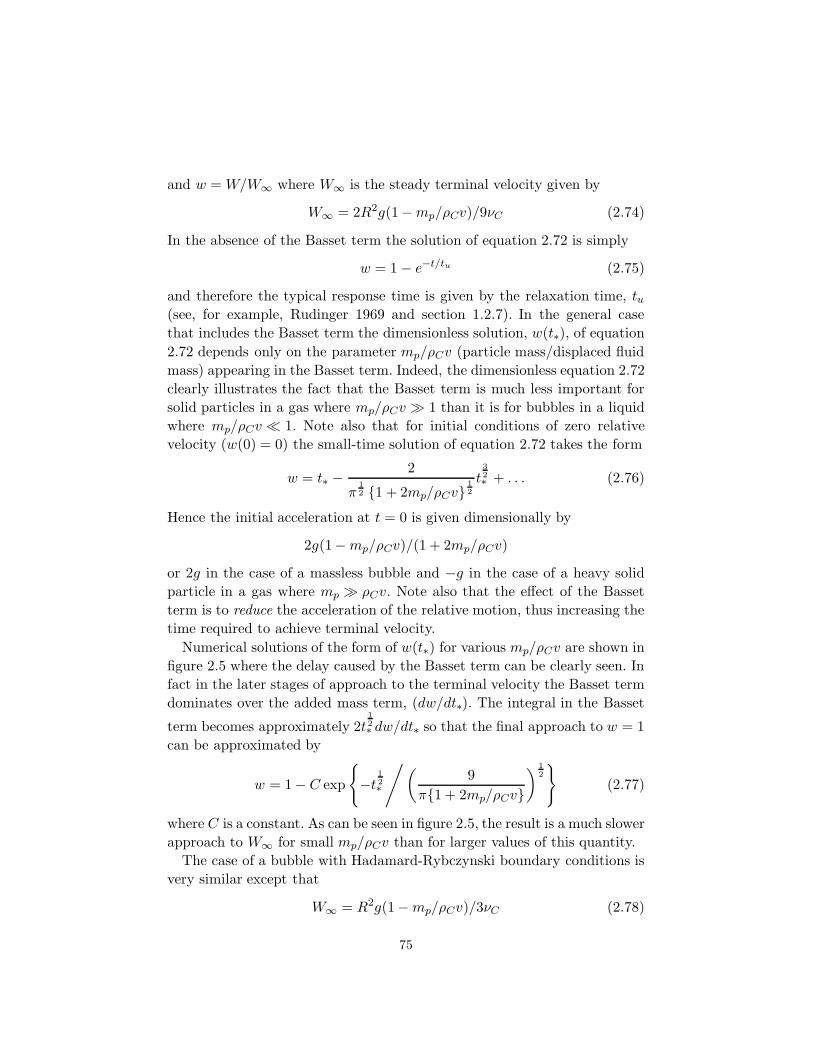
Numerical solutions of the form of w(t∗) for various mp/ρCv are shown infigure 2.5 where the delay caused by the Basset term can be clearly seen. Infact in the later stages of approach to the terminal velocity the Basset termdominates over the added mass term, (dw/dt∗). The integral in the Basset

term becomes approximately 2t12∗ dw/dt∗ so that the final approach to w = 1

can be approximated by

w = 1− C exp

{−t

12∗

/(9

π{1 + 2mp/ρCv}) 1

2

}(2.77)

where C is a constant. As can be seen in figure 2.5, the result is a much slowerapproach to W∞ for small mp/ρCv than for larger values of this quantity.

The case of a bubble with Hadamard-Rybczynski boundary conditions isvery similar except that

W∞ = R2g(1−mp/ρCv)/3νC (2.78)

75

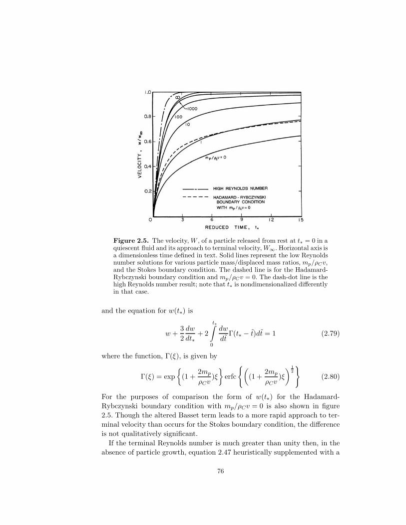
Figure 2.5. The velocity, W , of a particle released from rest at t∗ = 0 in aquiescent fluid and its approach to terminal velocity,W∞. Horizontal axis isa dimensionless time defined in text. Solid lines represent the low Reynoldsnumber solutions for various particle mass/displaced mass ratios, mp/ρCv,and the Stokes boundary condition. The dashed line is for the Hadamard-Rybczynski boundary condition and mp/ρCv = 0. The dash-dot line is thehigh Reynolds number result; note that t∗ is nondimensionalized differentlyin that case.

and the equation for w(t∗) is

w +32dw

dt∗+ 2

t∗∫0

dw

dtΓ(t∗ − t)dt = 1 (2.79)

where the function, Γ(ξ), is given by

Γ(ξ) = exp{

(1 +2mp

ρCv)ξ}

erfc

{((1 +

2mp

ρCv)ξ)1

2

}(2.80)

For the purposes of comparison the form of w(t∗) for the Hadamard-Rybczynski boundary condition with mp/ρCv = 0 is also shown in figure2.5. Though the altered Basset term leads to a more rapid approach to ter-minal velocity than occurs for the Stokes boundary condition, the differenceis not qualitatively significant.

If the terminal Reynolds number is much greater than unity then, in theabsence of particle growth, equation 2.47 heuristically supplemented with a

76

drag force of the form of equation 2.49 leads to the following equation ofmotion for unidirectional motion:

w2 +dw

dt∗= 1 (2.81)

where w = W/W∞, t∗ = t/tu, and the relaxation time, tu, is now given by

tu = (1 + 2mp/ρCv)(2R/3CDg(1−mp/vρC))12 (2.82)

and

W∞ = {8Rg(1−mp/ρCv)/3CD}12 (2.83)

The solution to equation 2.81 for w(0) = 0,

w = tanh t∗ (2.84)

is also shown in figure 2.5 though, of course, t∗ has a different definition inthis case.

The relaxation times given by the expressions 2.73 and 2.82 are partic-ularly valuable in assessing relative motion in disperse multiphase flows.When this time is short compared with the typical time associated with thefluid motion, the particle will essentially follow the fluid motion and thetechniques of homogeneous flow (see chapter 9) are applicable. Otherwisethe flow is more complex and special effort is needed to evaluate the relativemotion and its consequences.

For the purposes of reference in section 3.2 note that, if we define aReynolds number, Re, and a Froude number, Fr, by

Re =2W∞RνC

; Fr =W∞

{2Rg(1−mp/ρCv)}12

(2.85)

then the expressions for the terminal velocities, W∞, given by equations2.74, 2.78, and 2.83 can be written as

Fr = (Re/18)12 , Fr = (Re/12)

12 , and Fr = (4/3CD)

12 (2.86)

respectively. Indeed, dimensional analysis of the governing Navier-Stokesequations requires that the general expression for the terminal velocity canbe written as

F (Re, Fr) = 0 (2.87)

or, alternatively, if CD is defined as 4/3Fr2, then it could be written as

F ∗(Re, CD) = 0 (2.88)

77

2.4.2 Magnitude of relative motion

Qualitative estimates of the magnitude of the relative motion in multiphaseflows can be made from the analyses of the last section. Consider a generalsteady fluid flow characterized by a velocity, U, and a typical dimension, �;it may, for example, be useful to visualize the flow in a converging nozzleof length, �, and mean axial velocity, U . A particle in this flow will experi-ence a typical fluid acceleration (or effective g) of U2/� for a typical timegiven by �/U and hence will develop a velocity, W , relative to the fluid. Inmany practical flows it is necessary to determine the maximum value of W(denoted by Wm) that could develop under these circumstances. To do so,one must first consider whether the available time, �/U , is large or smallcompared with the typical time, tu, required for the particle to reach itsterminal velocity as given by equation 2.73 or 2.82. If tu � �/U then Wm isgiven by equation 2.74, 2.78, or 2.83 for W∞ and qualitative estimates forWm/U would be(

1 − mp

ρCv

)(UR

νC

)(R

�

)and

(1 − mp

ρCv

) 12 1

C12D

(R

�

)12

(2.89)

when WR/νC � 1 and WR/νC � 1 respectively. We refer to this as thequasistatic regime. On the other hand, if tu � �/U , Wm can be estimatedas W∞�/Utu so that Wm/U is of the order of

2(1−mp/ρCv)(1 + 2mp/ρCv)

(2.90)

for all WR/νC . This is termed the transient regime.In practice, WR/νC will not be known in advance. The most meaningful

quantities that can be evaluated prior to any analysis are a Reynolds number,UR/νC , based on flow velocity and particle size, a size parameter

X =R

�|1− mp

ρCv| (2.91)

and the parameter

Y = | 1 − mp

ρCv|/(1 +

2mp

ρCv) (2.92)

The resulting regimes of relative motion are displayed graphically in figure2.6. The transient regime in the upper right-hand sector of the graph is

78

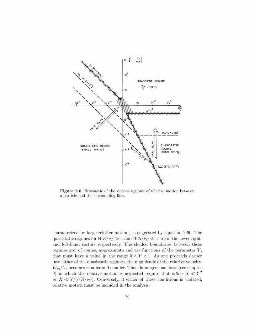
Figure 2.6. Schematic of the various regimes of relative motion betweena particle and the surrounding flow.

characterized by large relative motion, as suggested by equation 2.90. Thequasistatic regimes for WR/νC � 1 and WR/νC � 1 are in the lower right-and left-hand sectors respectively. The shaded boundaries between theseregimes are, of course, approximate and are functions of the parameter Y ,that must have a value in the range 0 < Y < 1. As one proceeds deeperinto either of the quasistatic regimes, the magnitude of the relative velocity,Wm/U , becomes smaller and smaller. Thus, homogeneous flows (see chapter9) in which the relative motion is neglected require that either X � Y 2

or X � Y/(UR/νC). Conversely, if either of these conditions is violated,relative motion must be included in the analysis.

79

2.4.3 Effect of concentration on particle equation of motion

When the concentration of the disperse phase in a multiphase flow is small(less than, say, 0.01% by volume) the particles have little effect on the motionof the continuous phase and analytical or computational methods are muchsimpler. Quite accurate solutions are then obtained by solving a single phaseflow for the continuous phase (perhaps with some slightly modified density)and inputting those fluid velocities into equations of motion for the particles.This is known as one-way coupling.

As the concentration of the disperse phase is increased a whole spectrumof complications can arise. These may effect both the continuous phase flowand the disperse phase motions and flows with this two-way coupling posemany modeling challenges. A few examples are appropriate. The particlemotions may initiate or alter the turbulence in the continuous phase flow;this particularly challenging issue is briefly addressed in section 1.3. More-over, particles may begin to collide with one another, altering their effectiveequation of motion and introducing random particle motions that may needto be accounted for; chapter 13 is devoted to flows dominated by such col-lisions. These collisions and random motions may generate additional tur-bulent motions in the continuous phase. Often the interactions of particlesbecome important even if they do not actually collide. Fortes et al. (1987)have shown that in flows with high relative Reynolds numbers there are sev-eral important mechanisms of particle-particle interactions that occur whena particle encounters the wake of another particle. The following particledrafts the leading particle, impacts it when it catches up with it and thepair then begin tumbling. In packed beds these interactions result in thedevelopment of lateral bands of higher concentration separated by regionsof low, almost zero volume fraction. How these complicated interactionscould be incorporated into a two-fluid model (short of complete and directnumerical simulation) is unclear.

At concentrations that are sufficiently small so that the complicationsof the preceding paragraph do not arise, there are still effects upon thecoefficients in the particle equation of motion that may need to be accountedfor. For example, the drag on a particle or the added mass of a particlemay be altered by the presence of neighboring particles. These issues aresomewhat simpler to deal with than those of the preceding paragraph andwe cover them in this chapter. The effect on the added mass was addressedearlier in section 2.3.2. In the next section we address the issue of the effectof concentration on the particle drag.

80

2.4.4 Effect of concentration on particle drag

Section 2.2 reviewed the dependence of the drag coefficient on the Reynoldsnumber for a single particle in a fluid and the effect on the sedimentation ofthat single particle in an otherwise quiescent fluid was examined as a partic-ular example in subsection 2.4. Such results would be directly applicable tothe evaluation of the relative velocity between the disperse phase (the parti-cles) and the continuous phase in a very dilute multiphase flow. However, athigher concentrations, the interactions between the flow fields around indi-vidual particles alter the force experienced by those particles and thereforechange the velocity of sedimentation. Furthermore, the volumetric flux ofthe disperse phase is no longer negligible because of the finite concentra-tion and, depending on the boundary conditions in the particular problem,this may cause a non-negligible volumetric flux of the continuous phase.For example, particles sedimenting in a containing vessel with a downwardparticle volume flux, −jS (upward is deemed the positive direction), at aconcentration, α, will have a mean velocity,

−uS = −jS/α (2.93)

and will cause an equal and opposite upward flux of the suspending liquid,jL = −jS, so that the mean velocity of the liquid,

uL = jL/(1 − α) = −jS/(1− α) (2.94)

Hence the relative velocity is

uSL = uS − uL = jS/α(1− α) = uS/(1− α) (2.95)

Thus care must be taken to define the terminal velocity and here we shallfocus on the more fundamental quantity, namely the relative velocity, uSL,rather than quantities such as the sedimentation velocity, uS , that are de-pendent on the boundary conditions.

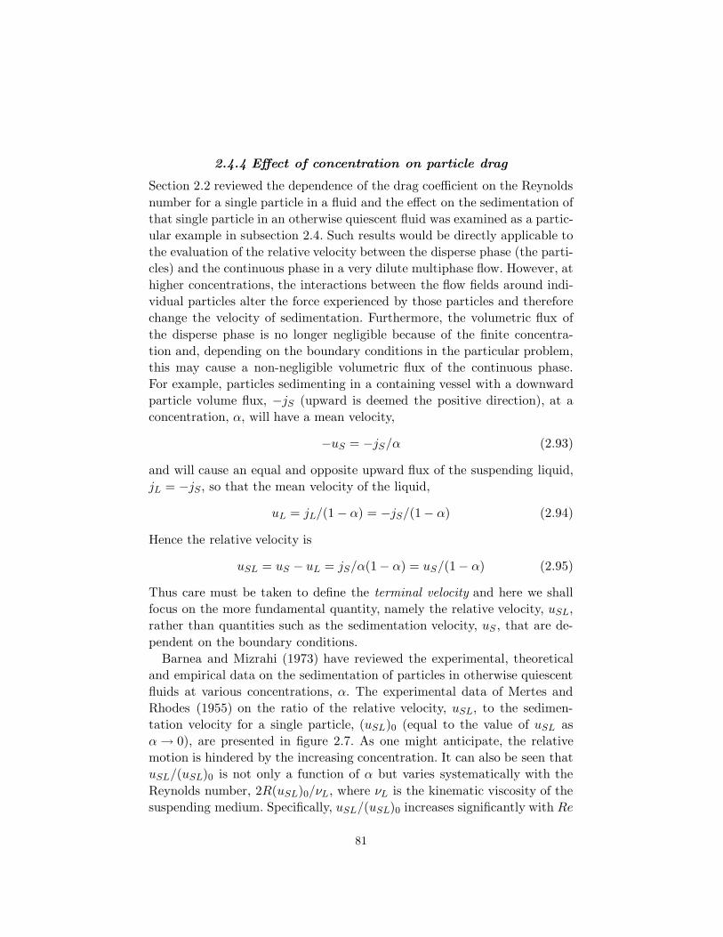
Barnea and Mizrahi (1973) have reviewed the experimental, theoreticaland empirical data on the sedimentation of particles in otherwise quiescentfluids at various concentrations, α. The experimental data of Mertes andRhodes (1955) on the ratio of the relative velocity, uSL, to the sedimen-tation velocity for a single particle, (uSL)0 (equal to the value of uSL asα→ 0), are presented in figure 2.7. As one might anticipate, the relativemotion is hindered by the increasing concentration. It can also be seen thatuSL/(uSL)0 is not only a function of α but varies systematically with theReynolds number, 2R(uSL)0/νL, where νL is the kinematic viscosity of thesuspending medium. Specifically, uSL/(uSL)0 increases significantly with Re

81

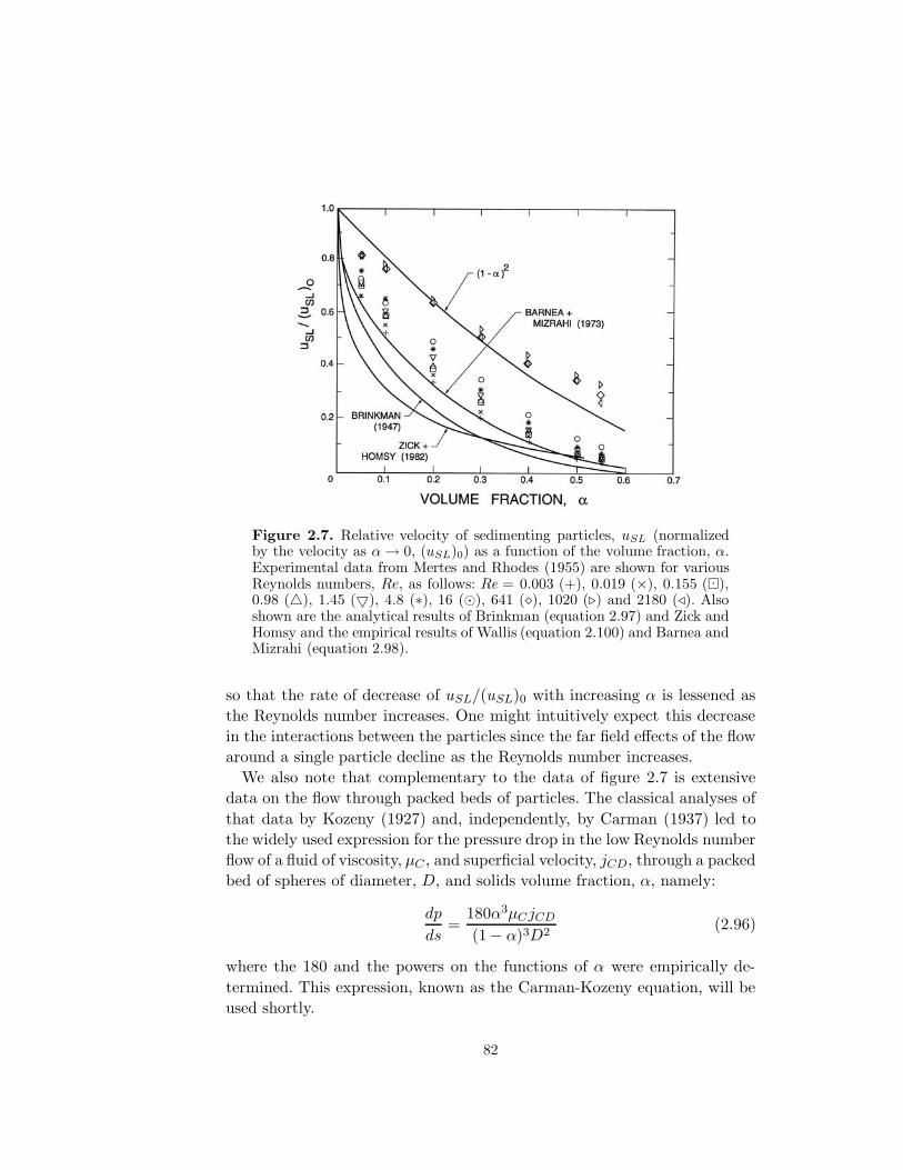
Figure 2.7. Relative velocity of sedimenting particles, uSL (normalizedby the velocity as α→ 0, (uSL)0) as a function of the volume fraction, α.Experimental data from Mertes and Rhodes (1955) are shown for variousReynolds numbers, Re, as follows: Re = 0.003 (+), 0.019 (×), 0.155 (�),0.98 (�), 1.45 (�), 4.8 (∗), 16 (�), 641 (�), 1020 (�) and 2180 (�). Alsoshown are the analytical results of Brinkman (equation 2.97) and Zick andHomsy and the empirical results of Wallis (equation 2.100) and Barnea andMizrahi (equation 2.98).

so that the rate of decrease of uSL/(uSL)0 with increasing α is lessened asthe Reynolds number increases. One might intuitively expect this decreasein the interactions between the particles since the far field effects of the flowaround a single particle decline as the Reynolds number increases.

We also note that complementary to the data of figure 2.7 is extensivedata on the flow through packed beds of particles. The classical analyses ofthat data by Kozeny (1927) and, independently, by Carman (1937) led tothe widely used expression for the pressure drop in the low Reynolds numberflow of a fluid of viscosity, μC , and superficial velocity, jCD, through a packedbed of spheres of diameter, D, and solids volume fraction, α, namely:

dp

ds=

180α3μCjCD

(1− α)3D2(2.96)

where the 180 and the powers on the functions of α were empirically de-termined. This expression, known as the Carman-Kozeny equation, will beused shortly.

82

Several curves that are representative of the analytical and empirical re-sults are also shown in figure 2.7 (and in figure 2.8). One of the first ap-proximate, analytical models to include the interactions between particleswas that of Brinkman (1947) for spherical particles at asymptotically smallReynolds numbers who obtained

uSL

(uSL)0=

(2 − 3α)2

4 + 3α+ 3(8α− 3α2)12

(2.97)

and this result is included in figures 2.7 and 2.8. Other researchers (see,for example, Tam 1969 and Brady and Bossis 1988) have studied this lowReynolds number limit quite closely. Exact solutions for the sedimentationvelocity of a various regular arrays of spheres at asymptotically low Reynoldsnumber were obtained by Zick and Homsy (1982) and the particular resultfor a simple cubic array is included in figure 2.7. Clearly, these results deviatesignificantly from the experimental data and it is currently thought thatthe sedimentation process cannot be modeled by a regular array becausethe fluid mechanical effects are dominated by the events that occur whenparticles happen to come close to one another.

Switching attention to particle Reynolds numbers greater than unity, itwas mentioned earlier that the work of Fortes et al. (1987) and others hasillustrated that the interactions between particles become very complex sincethey result, primarily, from the interactions of particles with the wakes ofthe particles ahead of them. Fortes et al. (1987) have shown this results ina variety of behaviors they term drafting, kissing and tumbling that can berecognized in fluidized beds. As yet, these behaviors have not been amenableto theoretical analyses.

The literature contains numerous empirical correlations but three willsuffice for present purposes. At small Reynolds numbers, Barnea and Mizrahi(1973) show that the experimental data closely follow an expression of theform

uSL

(uSL)0≈ (1 − α)

(1 + α13 )e5α/3(1−α)

(2.98)

By way of comparison the Carman-Kozeny equation 2.96 implies that asedimenting packed bed would have a terminal velocity given by

uSL

(uSL)0=

180

(1 − α)2

α2(2.99)

which has magnitudes comparable to the expression 2.98 at the volumefractions of packed beds.

83

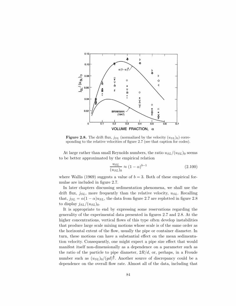
Figure 2.8. The drift flux, jSL (normalized by the velocity (uSL)0) corre-sponding to the relative velocities of figure 2.7 (see that caption for codes).

At large rather than small Reynolds numbers, the ratio uSL/(uSL)0 seemsto be better approximated by the empirical relation

uSL

(uSL)0≈ (1− α)b−1 (2.100)

where Wallis (1969) suggests a value of b = 3. Both of these empirical for-mulae are included in figure 2.7.

In later chapters discussing sedimentation phenomena, we shall use thedrift flux, jSL, more frequently than the relative velocity, uSL. Recallingthat, jSL = α(1 − α)uSL, the data from figure 2.7 are replotted in figure 2.8to display jSL/(uSL)0.

It is appropriate to end by expressing some reservations regarding thegenerality of the experimental data presented in figures 2.7 and 2.8. At thehigher concentrations, vertical flows of this type often develop instabilitiesthat produce large scale mixing motions whose scale is of the same order asthe horizontal extent of the flow, usually the pipe or container diameter. Inturn, these motions can have a substantial effect on the mean sedimenta-tion velocity. Consequently, one might expect a pipe size effect that wouldmanifest itself non-dimensionally as a dependence on a parameter such asthe ratio of the particle to pipe diameter, 2R/d, or, perhaps, in a Froudenumber such as (uSL)0/(gd)

12 . Another source of discrepancy could be a

dependence on the overall flow rate. Almost all of the data, including that

84

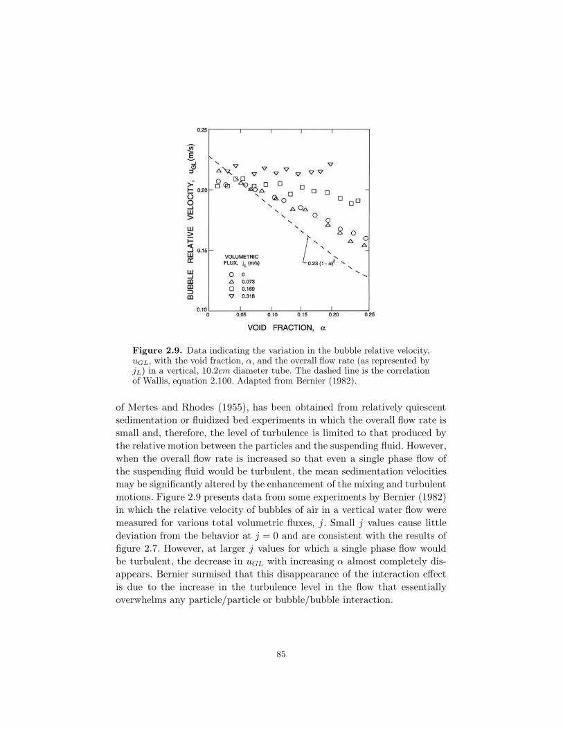
Figure 2.9. Data indicating the variation in the bubble relative velocity,uGL, with the void fraction, α, and the overall flow rate (as represented byjL) in a vertical, 10.2cm diameter tube. The dashed line is the correlationof Wallis, equation 2.100. Adapted from Bernier (1982).

of Mertes and Rhodes (1955), has been obtained from relatively quiescentsedimentation or fluidized bed experiments in which the overall flow rate issmall and, therefore, the level of turbulence is limited to that produced bythe relative motion between the particles and the suspending fluid. However,when the overall flow rate is increased so that even a single phase flow ofthe suspending fluid would be turbulent, the mean sedimentation velocitiesmay be significantly altered by the enhancement of the mixing and turbulentmotions. Figure 2.9 presents data from some experiments by Bernier (1982)in which the relative velocity of bubbles of air in a vertical water flow weremeasured for various total volumetric fluxes, j. Small j values cause littledeviation from the behavior at j = 0 and are consistent with the results offigure 2.7. However, at larger j values for which a single phase flow wouldbe turbulent, the decrease in uGL with increasing α almost completely dis-appears. Bernier surmised that this disappearance of the interaction effectis due to the increase in the turbulence level in the flow that essentiallyoverwhelms any particle/particle or bubble/bubble interaction.

85