the obstacle-restriction method (orm) for reactive … · avoidance in difficult scenarios in...

The Obstacle-Restriction

Method (ORM) for Reactive Obstacle Avoidance in Difficult Scenarios

in Three-Dimensional Workspaces

D A N I E L V I K E N M A R K

Master of Science Thesis Stockholm, Sweden 2006

The Obstacle-Restriction

Method (ORM) for Reactive Obstacle Avoidance in Difficult Scenarios

in Three-Dimensional Workspaces

D A N I E L V I K E N M A R K

Master’s Thesis in Computer Science (20 credits) at the School of Electrical Engineering Royal Institute of Technology year 2006 Supervisor at CSC was Henrik Christensen Examiner was Henrik Christensen TRITA-CSC-E 2006:172 ISRN-KTH/CSC/E--06/172--SE ISSN-1653-5715 Royal Institute of Technology School of Computer Science and Communication KTH CSC SE-100 44 Stockholm, Sweden URL: www.csc.kth.se

Abstract

This master’s project addresses the obstacle avoidance problem in difficult scenarios inthree-dimensional workspaces.

The main contribution of this project is the theoretical extension of the Obstacle-Restriction Method (ORM) in two dimensions to work in 3D workspaces.

This master’s thesis describes a reactive obstacle avoidance technique to drive a robot indense, cluttered and complex environments in three-dimensional workspaces. The methodhas two steps: First a procedure computes instantaneous sub goals in the obstacle structure,second a motion restriction is associated with each obstacle which next are managed tocompute the most promising direction of motion.

The advantage with the ORM, regarding the obstacle avoidance problem, is that itavoids the problems and limitations common in other obstacle avoidance methods, leadingto improved navigation results in difficult scenarios. This is confirmed by simulations madein difficult scenarios in three-dimensional workspaces.

Sammanfattning

Hinderrestriktionsmetoden ORM för reaktiv hinderdetektion i komplicerade scenarion i tre-dimensionella arbetsmiljöer

Det här examensarbetet behandlar hinderdetektionsproblemet i komplicerade scenarion itredimensionella arbetsmiljöer.

Det största bidraget med det här examensarbetet är den teoretiska utökningen av me-toden ORM i aspekten utav restrikterad hinderdetektion i tredimensionella arbetsmiljöer.

Denna rapport beskriver en teknik för att styra en robot i komplexa, tredimensionellaarbetsmiljöer. Metoden har två steg: Först är det en procedur som placerar ut delmålbland hinderstrukturen, sedan associeras en rörelserestriktion till varje hinder vilka till sistbehandlas för att räkna ut den mest lovade rörelseriktningen.

Fördelen med hinderrestriktionsmetoden, med avseende på hinderdetektionsproblemet,är att denna metod löser de problem och begränsningar som andra hinderdetektionsmetoderhar. Detta leder till förbättrade navigeringsresultat i svåra arbetsmiljöer. Dessutom löserden föreslagna metoden hinderdetektionsproblemet i tredimensionella arbetsmiljöer. Dettabekräftas av simuleringar utförda i komplicerade scenarion i tredimensionella arbetsmiljöer.

Acknowledgments

The Department of Signals Sensors and System (S3) and the Centre for AutonomousSystems (CAS) at the Royal Institute of Technology (KTH) in Stockholm have aSTINT sponsored collaboration with the Robotics, Perception and Real Time Group(RoPeRT) at the University of Zaragoza, Spain. This master’s project was donewithin this collaboration at the University of Zaragoza, Spain, during the academicyear 2004/2005.

First of all, I would like to thank my supervisor at RoPeRT, Ph.D JavierMinguez, with whom I have worked very close. Thank you for all the help withthis project.

Also, I would like to thank my examiner at KTH Prof. Henrik I. Christensenand Prof. Bo Wahlberg for giving me the opportunity to do my master’s project inZaragoza; Richard W Carlson and his daughter Hadley for proofreading the thesis;and finally, the Swedish Foundation for International Cooperation in Research andHigher Education (STINT) for the scholarship I recieved for this project.

Contents

1 Introduction 1

2 Related Work 32.1 Potential Field Methods (PFM) . . . . . . . . . . . . . . . . . . . . . 42.2 Vector Field Histogram (VFH) . . . . . . . . . . . . . . . . . . . . . 52.3 Nearness Diagram Navigation (ND) . . . . . . . . . . . . . . . . . . 62.4 Obstacle-Restriction Method (ORM) . . . . . . . . . . . . . . . . . . 82.5 Why the ORM? . . . . . . . . . . . . . . . . . . . . . . . . . . . . . . 9

3 The Obstacle-Restriction Method (ORM) in Three DimensionalWorkspaces 113.1 Problem Representation . . . . . . . . . . . . . . . . . . . . . . . . . 113.2 Sub Goal Selector . . . . . . . . . . . . . . . . . . . . . . . . . . . . . 133.3 Motion Computation . . . . . . . . . . . . . . . . . . . . . . . . . . . 18

3.3.1 Portions of the Space (subspaces) . . . . . . . . . . . . . . . . 183.3.2 The motion constraints . . . . . . . . . . . . . . . . . . . . . 203.3.3 Selecting the direction of motion . . . . . . . . . . . . . . . . 25

3.4 Computing the Robot Motion . . . . . . . . . . . . . . . . . . . . . . 33

4 Simulation Results 354.1 Simulation Settings . . . . . . . . . . . . . . . . . . . . . . . . . . . . 354.2 Simulations . . . . . . . . . . . . . . . . . . . . . . . . . . . . . . . . 35

5 Discussion 41

6 Conclusions 43

Bibliography 45

Appendix A 47

Chapter 1

Introduction

A large section of robotics is currently focused on the development of applicationswhere a vehicle performs in unknown, unstructured and dynamic scenarios. Anexample is in an office where a robot moves among chairs, tables, shelves anddoorways (which locations are unknown for the robot) and humans (who makethe scenario highly dynamic). Another example is a submarine robot exploring anUnderwater canyon (which is an unknown, unstructured and dynamic scenario). Todrive a vehicle in a complex and evolving scenario, like the two examples, the vehicleneeds a reactive system that can adapt the motion to any new contingency or event.The natural choice seems to be the obstacle avoidance methods which react on thesensory information within the control cycle. However, most of these methods runinto difficulties in various scenarios. A classic drawback for the reactive approachesis the local minima situations due to motion between very close obstacles or dueto U-shaped obstacles. This means that most of these methods cannot carry outrobust or trustworthy navigation in complex evolving scenarios.

Recently two methods have been developed, the Nearness Diagram (ND) Nav-igation [16] and the Obstacle Restriction Method (ORM) [15], that overcome thedifficult situations in obstacle avoidance. These methods are both able to success-fully drive a vehicle in an unknown, unstructured and dynamic scenario.

Although there are some techniques that have been used in three dimensionalworkspaces, they inherit the limitations of the two dimensional case. Thus, if onewants to perform 3D obstacle avoidance in complex scenarios, an extension of eitherthe Nearness Diagram or the Obstacle Restriction method would be a good choice.Unfortunately, there is no extension of these methods for 3D workspaces. As aresult the motion problem in the second example (the underwater canyon) cannotbe solved with today’s obstacle avoidance methods. This master’s project addressesthis problem: Reactive obstacle avoidance in very dense, complex and cluttered threedimensional workspaces.

The design is an extension of an already existing method, the ORM, that exhibitsgood results when performing in two dimensions. When extending this method fromtwo dimensions to three dimensions the existing advantages and disadvantages are

1

CHAPTER 1. INTRODUCTION

assumed to be inherited. Therefore the goal of the present work is to develop amethod for 3D navigation with the same results as achieved in 2D. In particular themethod should be able to overcome classical limitations of existing methods suchas:

• avoid trap situations due to the perceived environmental structure, e.g. U-shaped obstacles and very close obstacles

• compute stable and oscillation free motion,

• exhibit a high goal insensitivity, i.e. to be able to choose directions of motionfar away from the goal direction,

• be able to select motion directions towards obstacles.

This project strictly deals with the theoretical aspects of extending the methodto three-dimensional workspaces. Thus, related issues such as shape, kinematicsand dynamics of the vehicle and integration of the method are not within the frameof this work.

The outline of the thesis is as follows: Related work is presented in Chapter 2,the design of the extension of the ORM is presented in Chapter 3, the simulationresults are presented in Chapter 4 which is followed by a discussion in Chapter 5,and in Chapter 6 I draw my conclusions.

2

Chapter 2

Related Work

This chapter presents the obstacle avoidance problem, a classification [13] of obstacleavoidance techniques, some representative methods and a discussion regarding thechoice of the method.

In [13] the obstacle avoidance problem is formulated as:

The obstacle avoidance problem consists of moving a vehicle towardsa target location free of collisions with the obstacles detected by thesensors during the motion execution. This involves the sensor informa-tion within the control cycle adapting to the motion of any contingencyincompatible with initial plans.

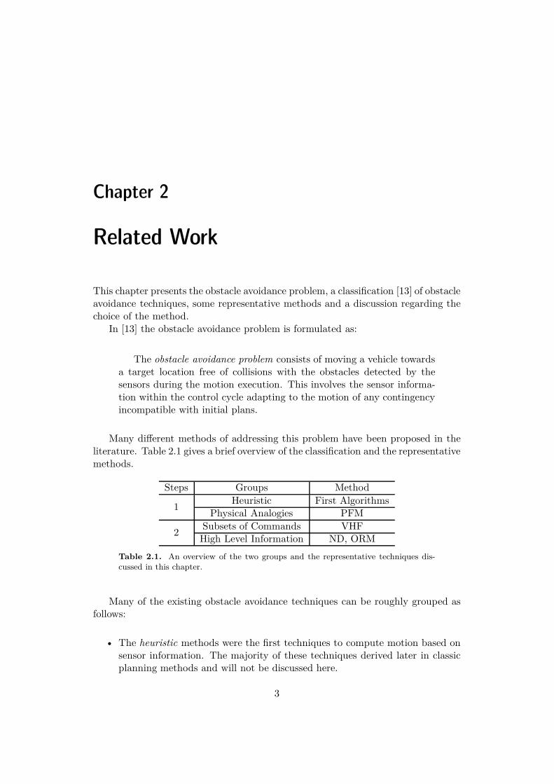
Many different methods of addressing this problem have been proposed in theliterature. Table 2.1 gives a brief overview of the classification and the representativemethods.

Steps Groups Method

1 Heuristic First AlgorithmsPhysical Analogies PFM

2 Subsets of Commands VHFHigh Level Information ND, ORM

Table 2.1. An overview of the two groups and the representative techniques dis-cussed in this chapter.

Many of the existing obstacle avoidance techniques can be roughly grouped asfollows:

• The heuristic methods were the first techniques to compute motion based onsensor information. The majority of these techniques derived later in classicplanning methods and will not be discussed here.

3

CHAPTER 2. RELATED WORK

Ftot

Fatt

Frep

Robot

Obstacle Target

(a)

0 0.5 1 1.5 2 2.5 30

0.5

1

1.5

2

2.5

3

Target

(b)

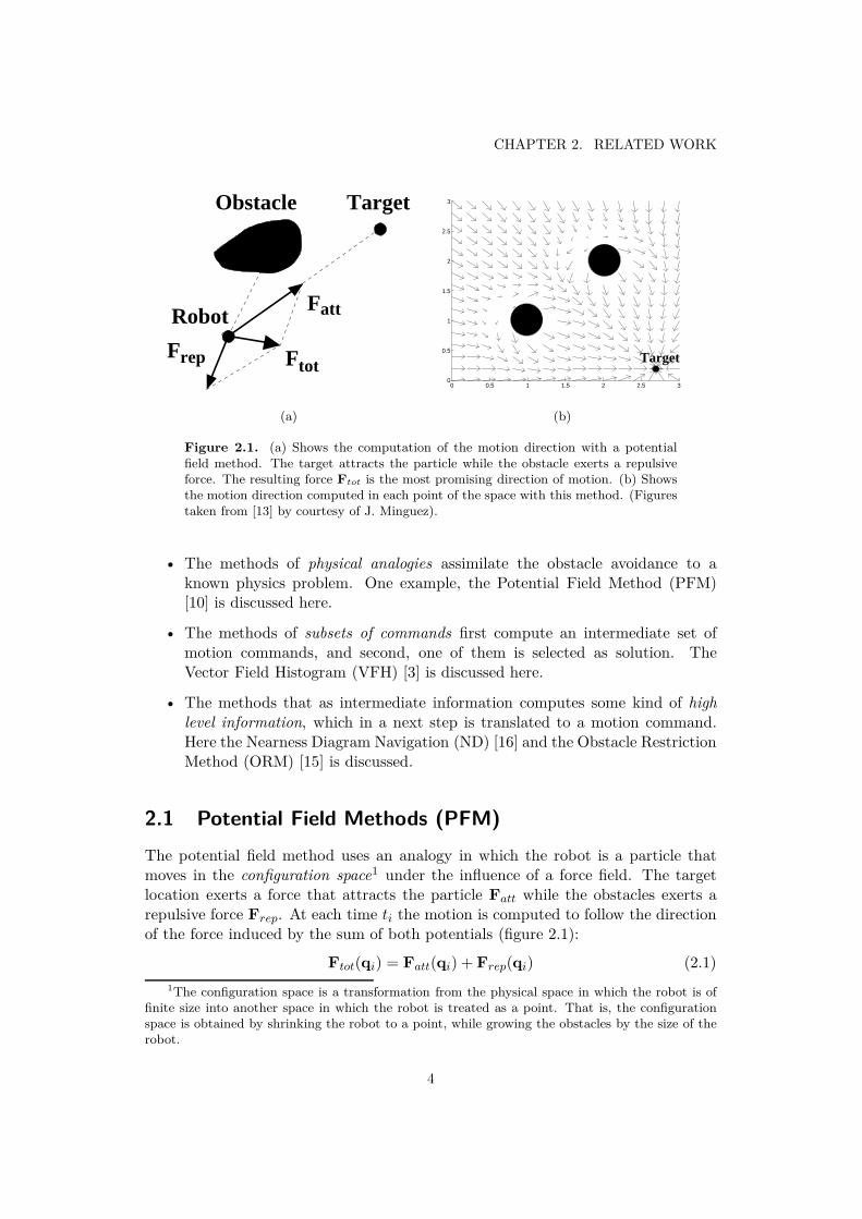
Figure 2.1. (a) Shows the computation of the motion direction with a potentialfield method. The target attracts the particle while the obstacle exerts a repulsiveforce. The resulting force Ftot is the most promising direction of motion. (b) Showsthe motion direction computed in each point of the space with this method. (Figurestaken from [13] by courtesy of J. Minguez).

• The methods of physical analogies assimilate the obstacle avoidance to aknown physics problem. One example, the Potential Field Method (PFM)[10] is discussed here.

• The methods of subsets of commands first compute an intermediate set ofmotion commands, and second, one of them is selected as solution. TheVector Field Histogram (VFH) [3] is discussed here.

• The methods that as intermediate information computes some kind of highlevel information, which in a next step is translated to a motion command.Here the Nearness Diagram Navigation (ND) [16] and the Obstacle RestrictionMethod (ORM) [15] is discussed.

2.1 Potential Field Methods (PFM)The potential field method uses an analogy in which the robot is a particle thatmoves in the configuration space1 under the influence of a force field. The targetlocation exerts a force that attracts the particle Fatt while the obstacles exerts arepulsive force Frep. At each time ti the motion is computed to follow the directionof the force induced by the sum of both potentials (figure 2.1):

Ftot(qi) = Fatt(qi) + Frep(qi) (2.1)1The configuration space is a transformation from the physical space in which the robot is of

finite size into another space in which the robot is treated as a point. That is, the configurationspace is obtained by shrinking the robot to a point, while growing the obstacles by the size of therobot.

4

2.2. VECTOR FIELD HISTOGRAM (VFH)

(a) (b)

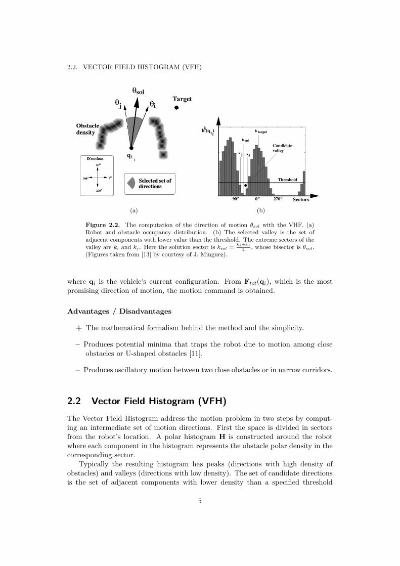
Figure 2.2. The computation of the direction of motion θsol with the VHF. (a)Robot and obstacle occupancy distribution. (b) The selected valley is the set ofadjacent components with lower value than the threshold. The extreme sectors of thevalley are ki and kj . Here the solution sector is ksol =

ki+kj

2, whose bisector is θsol.

(Figures taken from [13] by courtesy of J. Minguez).

where qi is the vehicle’s current configuration. From Ftot(qi), which is the mostpromising direction of motion, the motion command is obtained.

Advantages / Disadvantages

+ The mathematical formalism behind the method and the simplicity.

– Produces potential minima that traps the robot due to motion among closeobstacles or U-shaped obstacles [11].

– Produces oscillatory motion between two close obstacles or in narrow corridors.

2.2 Vector Field Histogram (VFH)The Vector Field Histogram address the motion problem in two steps by comput-ing an intermediate set of motion directions. First the space is divided in sectorsfrom the robot’s location. A polar histogram H is constructed around the robotwhere each component in the histogram represents the obstacle polar density in thecorresponding sector.

Typically the resulting histogram has peaks (directions with high density ofobstacles) and valleys (directions with low density). The set of candidate directionsis the set of adjacent components with lower density than a specified threshold

5


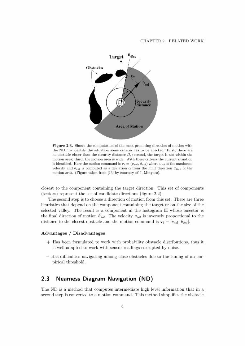
Figure 2.3. Shows the computation of the most promising direction of motion withthe ND. To identify the situation some criteria has to be checked: First, there areno obstacle closer than the security distance Ds; second, the target is not within themotion area; third, the motion area is wide. With these criteria the current situationis identified. Here the motion command is vi = (υsol, θsol) where υsol is the maximumvelocity and θsol is computed as a deviation α from the limit direction θdisc of themotion area. (Figure taken from [13] by courtesy of J. Minguez).

closest to the component containing the target direction. This set of components(sectors) represent the set of candidate directions (figure 2.2).

The second step is to choose a direction of motion from this set. There are threeheuristics that depend on the component containing the target or on the size of theselected valley. The result is a component in the histogram H whose bisector isthe final direction of motion θsol. The velocity vsol is inversely proportional to thedistance to the closest obstacle and the motion command is vi = [vsol, θsol].


+ Has been formulated to work with probability obstacle distributions, thus itis well adapted to work with sensor readings corrupted by noise.

– Has difficulties navigating among close obstacles due to the tuning of an em-pirical threshold.

2.3 Nearness Diagram Navigation (ND)The ND is a method that computes intermediate high level information that in asecond step is converted to a motion command. This method simplifies the obstacle

6

2.3. NEARNESS DIAGRAM NAVIGATION (ND)

x1

x2

x3

x4

x5

x6

xrobot

Obstacles perceivedGoal

(a)

x robot

A B

C−Obstacle

Obstacle perceived

P2R

Tunnelblocked

Goal

(b)

Tunnelblocked

Tunnelnot blocked

x 6

x 1

x robot

(c)

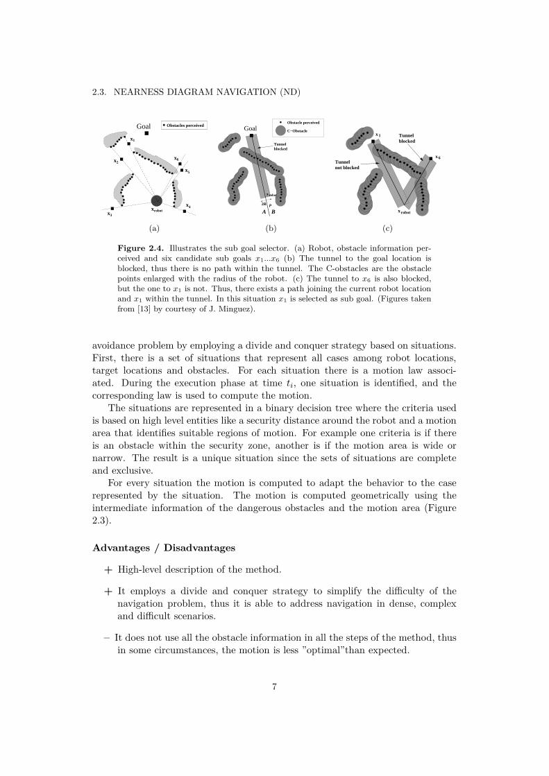
Figure 2.4. Illustrates the sub goal selector. (a) Robot, obstacle information per-ceived and six candidate sub goals x1...x6 (b) The tunnel to the goal location isblocked, thus there is no path within the tunnel. The C-obstacles are the obstaclepoints enlarged with the radius of the robot. (c) The tunnel to x6 is also blocked,but the one to x1 is not. Thus, there exists a path joining the current robot locationand x1 within the tunnel. In this situation x1 is selected as sub goal. (Figures takenfrom [13] by courtesy of J. Minguez).

avoidance problem by employing a divide and conquer strategy based on situations.First, there is a set of situations that represent all cases among robot locations,target locations and obstacles. For each situation there is a motion law associ-ated. During the execution phase at time ti, one situation is identified, and thecorresponding law is used to compute the motion.

The situations are represented in a binary decision tree where the criteria usedis based on high level entities like a security distance around the robot and a motionarea that identifies suitable regions of motion. For example one criteria is if thereis an obstacle within the security zone, another is if the motion area is wide ornarrow. The result is a unique situation since the sets of situations are completeand exclusive.

For every situation the motion is computed to adapt the behavior to the caserepresented by the situation. The motion is computed geometrically using theintermediate information of the dangerous obstacles and the motion area (Figure2.3).


+ High-level description of the method.

+ It employs a divide and conquer strategy to simplify the difficulty of thenavigation problem, thus it is able to address navigation in dense, complexand difficult scenarios.

– It does not use all the obstacle information in all the steps of the method, thusin some circumstances, the motion is less ”optimal”than expected.

7


S1

R+Ds

ObstacleTarget

(a)

2SR+Ds

R+Dsα

R+Ds

(b)

S1

S2x

Left boundφL

Target

(c)

S

SD

Right bound

Left bound

θSolution

θTarget

Rmax

Lmax

φ

φ

nD

(d)

DSRight bound

Left bound

θTarget

Lmax

Rmax

φ

φ

SnD

(e)

θSolution

SD

Right bound

Left boundLmax

Rmax

φ

φ

=

SnD

(f)

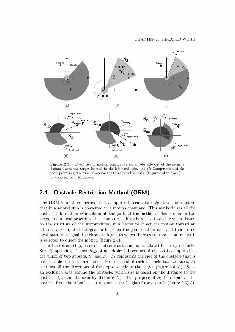
Figure 2.5. (a)–(c) Set of motion constraints for an obstacle out of the securitydistance with the target located in the left-hand side. (d)–(f) Computation of themost promising direction of motion the three possible cases. (Figures taken from [13]by courtesy of J. Minguez).

2.4 Obstacle-Restriction Method (ORM)The ORM is another method that computes intermediate high-level informationthat in a second step is converted to a motion command. This method uses all theobstacle information available in all the parts of the method. This is done in twosteps, first a local procedure that computes sub goals is used to decide when (basedon the structure of the surroundings) it is better to direct the motion toward analternative computed sub goal rather then the goal location itself. If there is nolocal path to the goal, the closest sub goal to which there exists a collision-free pathis selected to direct the motion (figure 2.4).

In the second step, a set of motion constraints is calculated for every obstacle.Strictly speaking, the set SnD of not desired directions of motion is computed asthe union of two subsets, S1 and S2. S1 represents the side of the obstacle that isnot suitable to do the avoidance. From the robot each obstacle has two sides, S1

contains all the directions of the opposite side of the target (figure 2.5(a)). S2 isan exclusion area around the obstacle, which size is based on the distance to theobstacle dobs and the security distance Ds. The purpose of S2 is to remove theobstacle from the robot’s security zone at the height of the obstacle (figure 2.5(b)).

8

2.5. WHY THE ORM?

The set SnD = S1 ∪S2 (figure 2.5(c)). Joining all the sets by all the obstacles givesthe full set of motion constraints SnD.

Finally, depending on the topology of SnD and the target direction there arethree cases (figure 2.5(d)–(f)) and in each of them one action law is executed com-puting the motion θsolution.


+ A strictly geometrical method.

+ Takes into account all the obstacle information in every part of the method.

+ Achieves safe navigation in dense, complex and difficult scenarios.

– ORM is a very young method that needs to be more mature to detect failuresor misbehaviors.

2.5 Why the ORM?The goal of this project is to design an obstacle avoidance method for motion indifficult scenarios in three-dimensional workspaces. The question that follows is:Why extend the Obstacle Restriction Method (ORM)?

There are two important things to consider:

1. The performance in two dimensions. If the method cannot drive a vehicle indifficult environments in two-dimensional workspaces it would not be able todrive it successfully in three-dimensional workspaces. The only two methodscapable of driving a vehicle in difficult environments are the ORM and the ND.The performances of ORM and ND are very similar. They achieve the sameresult when navigating in dense, complex and difficult scenarios, however,preliminarily it seems that ORM achieves better results in open spaces [15].

2. The formulation of the ORM. It is a big advantage if the method is geometricsince it seems possible to address an extension from two to three dimensions.On the other hand, the ND simplifies the obstacle avoidance problem byemploying a divide and conquer strategy based on situations. When extendingthe ND, it seems more intricate to find all the situations formulated in 3Dworkspaces and the formulation of all the associated actions to each situation.

9

Chapter 3

The Obstacle-Restriction Method(ORM) in Three DimensionalWorkspaces

This chapter presents the extension of the ORM to operate in 3D workspaces. Therobot is assumed to be spherical and holonomic. The obstacle information is givenin the form of mathematical points, which usually is the form in which sensor datais given (e.g. laser sensors).

This method like all other obstacle avoidance methods, is based on an iterativeperception – action process. Sensors collect information from the environment, theinformation is processed by the method to compute a motion command, the motionis executed by the robot and the process restarts. For the extension of the ORM,this process has three steps. First a local selector of sub goals decide (based on thestructure of the surroundings) if the motion should be directed toward the goal orif it is better to direct the motion toward another location in the space (subsection3.2). Second, a motion constraint is associated with each obstacle. These constraintsare managed next to compute the most promising direction of motion (subsection3.3). Third, the motion command given to the robot is computed (subsection 3.4).

3.1 Problem RepresentationIn this section we describe mathematical representations that will be used in theremainder of the project.

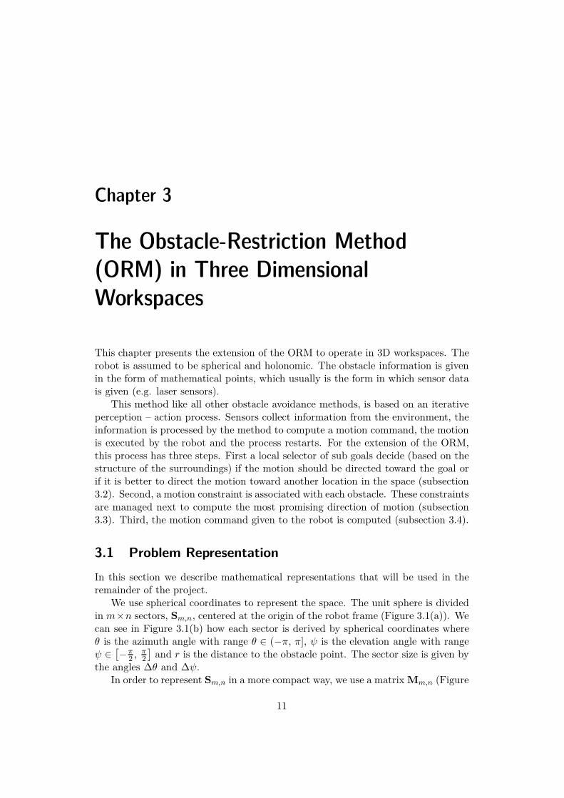
We use spherical coordinates to represent the space. The unit sphere is dividedin m×n sectors, Sm,n, centered at the origin of the robot frame (Figure 3.1(a)). Wecan see in Figure 3.1(b) how each sector is derived by spherical coordinates whereθ is the azimuth angle with range θ ∈ (−π, π], ψ is the elevation angle with rangeψ ∈ [−π

2 ,π2

]and r is the distance to the obstacle point. The sector size is given by

the angles ∆θ and ∆ψ.In order to represent Sm,n in a more compact way, we use a matrix Mm,n (Figure

11

CHAPTER 3. THE OBSTACLE-RESTRICTION METHOD (ORM) IN THREEDIMENSIONAL WORKSPACES

(a) (b)

Figure 3.1. Space representation used by the ORM. (a) The space is divided in m×nsectors, where the sector size is [∆θ, ∆ψ] (in the implementation ∆θ = ∆ψ = 3° whichgives m = 120 and n = 61 with a total of 7320 sectors). (b) Spherical coordinates[θ, ψ, r] are used. θ range from −π to π, ψ range from −π

2to π

2and r is the distance

to the obstacle.

(a)

ex −e

x

ez

−ez

ey −e

y

xz−plane yz−plane

xy−plane

θπ π\2 0 −π\2 −π

ψ

π\2

0

−π\2

xz−plane yz−plane

(b)

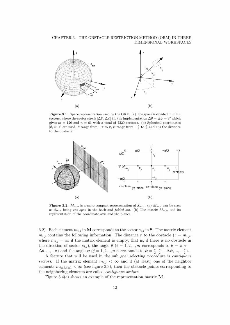
Figure 3.2. Mm,n is a more compact representation of Sm,n. (a) Mm,n can be seenas Sm,n being cut open in the back and folded out. (b) The matrix Mm,n and itsrepresentation of the coordinate axis and the planes.

3.2). Each element mi,j in M corresponds to the sector si,j in S. The matrix elementmi,j contains the following information: The distance r to the obstacle (r = mi,j,where mi,j = ∞ if the matrix element is empty, that is, if there is no obstacle inthe direction of sector si,j), the angle θ (i = 1, 2, ..,m corresponds to θ = π, π −∆θ, ...,−π) and the angle ψ (j = 1, 2, .., n corresponds to ψ = π

2 ,π2 − ∆ψ, ...,−π

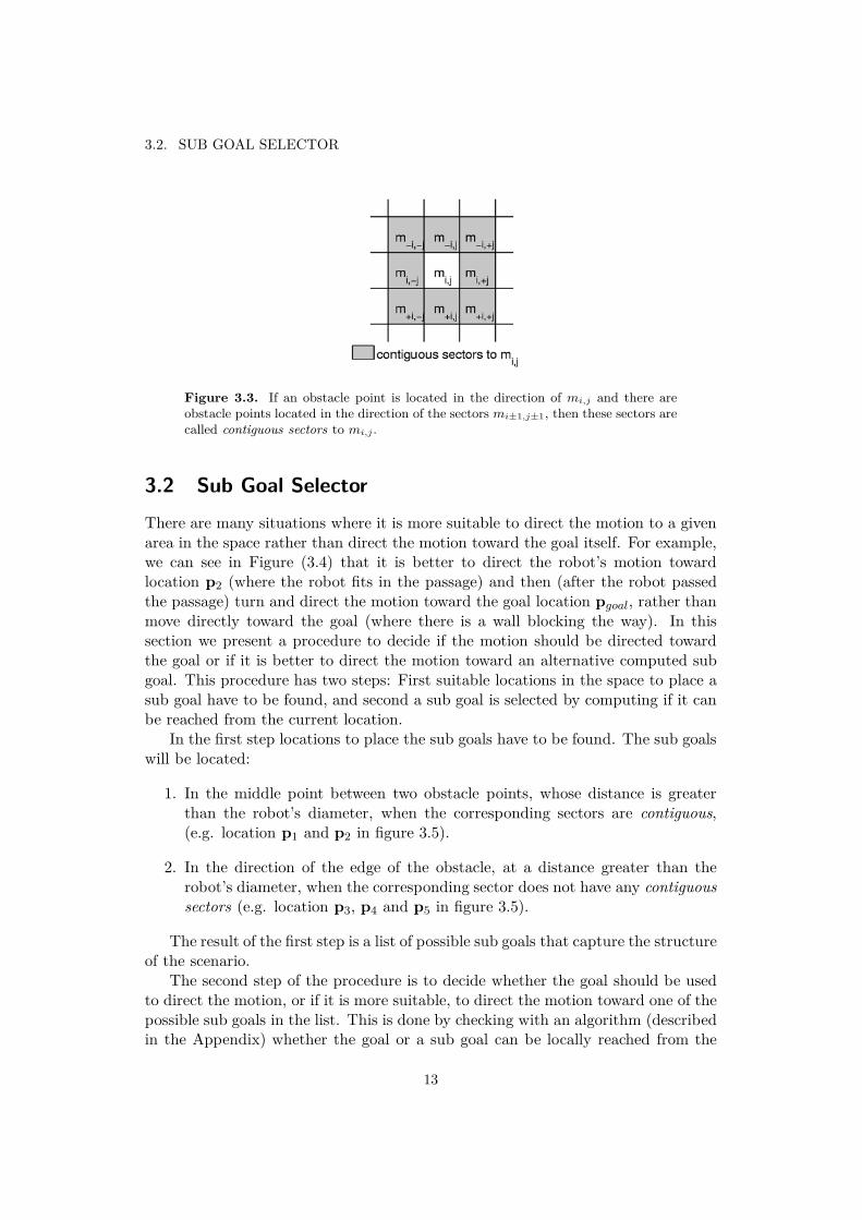
2 ).A feature that will be used in the sub goal selecting procedure is contiguous

sectors. If the matrix element mi,j < ∞ and if (at least) one of the neighborelements mi±1,j±1 < ∞ (see figure 3.3), then the obstacle points corresponding tothe neighboring elements are called contiguous sectors.

Figure 3.4(c) shows an example of the representation matrix M.

12

3.2. SUB GOAL SELECTOR

Figure 3.3. If an obstacle point is located in the direction of mi,j and there areobstacle points located in the direction of the sectors mi±1,j±1, then these sectors arecalled contiguous sectors to mi,j .

3.2 Sub Goal SelectorThere are many situations where it is more suitable to direct the motion to a givenarea in the space rather than direct the motion toward the goal itself. For example,we can see in Figure (3.4) that it is better to direct the robot’s motion towardlocation p2 (where the robot fits in the passage) and then (after the robot passedthe passage) turn and direct the motion toward the goal location pgoal, rather thanmove directly toward the goal (where there is a wall blocking the way). In thissection we present a procedure to decide if the motion should be directed towardthe goal or if it is better to direct the motion toward an alternative computed subgoal. This procedure has two steps: First suitable locations in the space to place asub goal have to be found, and second a sub goal is selected by computing if it canbe reached from the current location.

In the first step locations to place the sub goals have to be found. The sub goalswill be located:

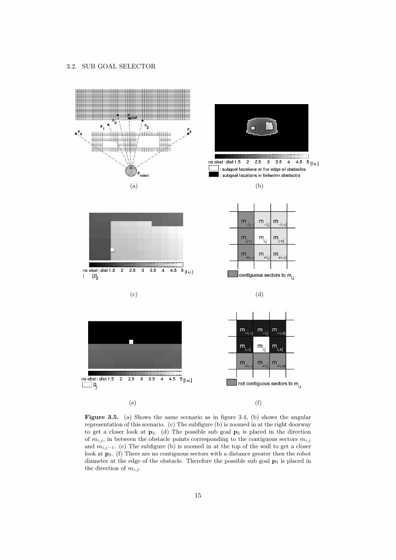
1. In the middle point between two obstacle points, whose distance is greaterthan the robot’s diameter, when the corresponding sectors are contiguous,(e.g. location p1 and p2 in figure 3.5).

2. In the direction of the edge of the obstacle, at a distance greater than therobot’s diameter, when the corresponding sector does not have any contiguoussectors (e.g. location p3, p4 and p5 in figure 3.5).

The result of the first step is a list of possible sub goals that capture the structureof the scenario.

The second step of the procedure is to decide whether the goal should be usedto direct the motion, or if it is more suitable, to direct the motion toward one of thepossible sub goals in the list. This is done by checking with an algorithm (describedin the Appendix) whether the goal or a sub goal can be locally reached from the

13


(a) (b)

(c)

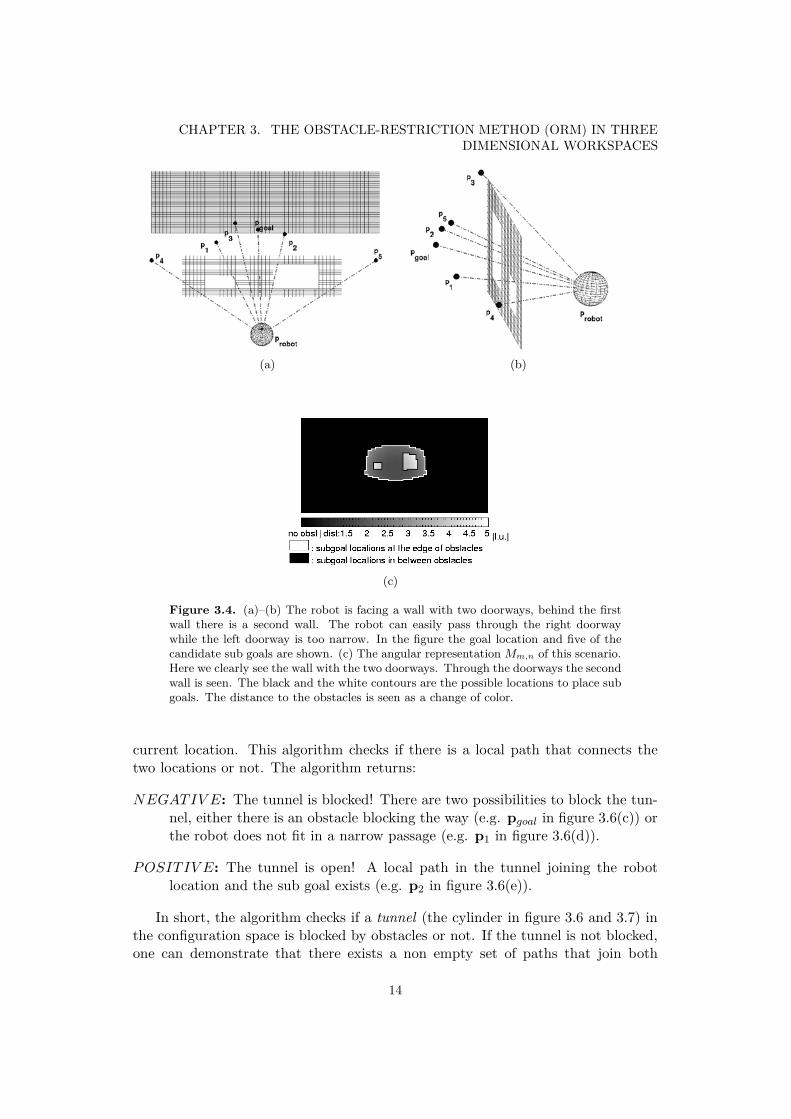
Figure 3.4. (a)–(b) The robot is facing a wall with two doorways, behind the firstwall there is a second wall. The robot can easily pass through the right doorwaywhile the left doorway is too narrow. In the figure the goal location and five of thecandidate sub goals are shown. (c) The angular representation Mm,n of this scenario.Here we clearly see the wall with the two doorways. Through the doorways the secondwall is seen. The black and the white contours are the possible locations to place subgoals. The distance to the obstacles is seen as a change of color.

current location. This algorithm checks if there is a local path that connects thetwo locations or not. The algorithm returns:

NEGATIV E: The tunnel is blocked! There are two possibilities to block the tun-nel, either there is an obstacle blocking the way (e.g. pgoal in figure 3.6(c)) orthe robot does not fit in a narrow passage (e.g. p1 in figure 3.6(d)).

POSITIV E: The tunnel is open! A local path in the tunnel joining the robotlocation and the sub goal exists (e.g. p2 in figure 3.6(e)).

In short, the algorithm checks if a tunnel (the cylinder in figure 3.6 and 3.7) inthe configuration space is blocked by obstacles or not. If the tunnel is not blocked,one can demonstrate that there exists a non empty set of paths that join both

14


(a) (b)

(c) (d)

(e) (f)

Figure 3.5. (a) Shows the same scenario as in figure 3.4, (b) shows the angularrepresentation of this scenario. (c) The subfigure (b) is zoomed in at the right doorwayto get a closer look at p2. (d) The possible sub goal p2 is placed in the directionof mi,j , in between the obstacle points corresponding to the contiguous sectors mi,j

and mi,j−1. (e) The subfigure (b) is zoomed in at the top of the wall to get a closerlook at p3. (f) There are no contiguous sectors with a distance greater then the robotdiameter at the edge of the obstacle. Therefore the possible sub goal p3 is placed inthe direction of mi,j .

15


(a) (b)

(c) (d)

(e)

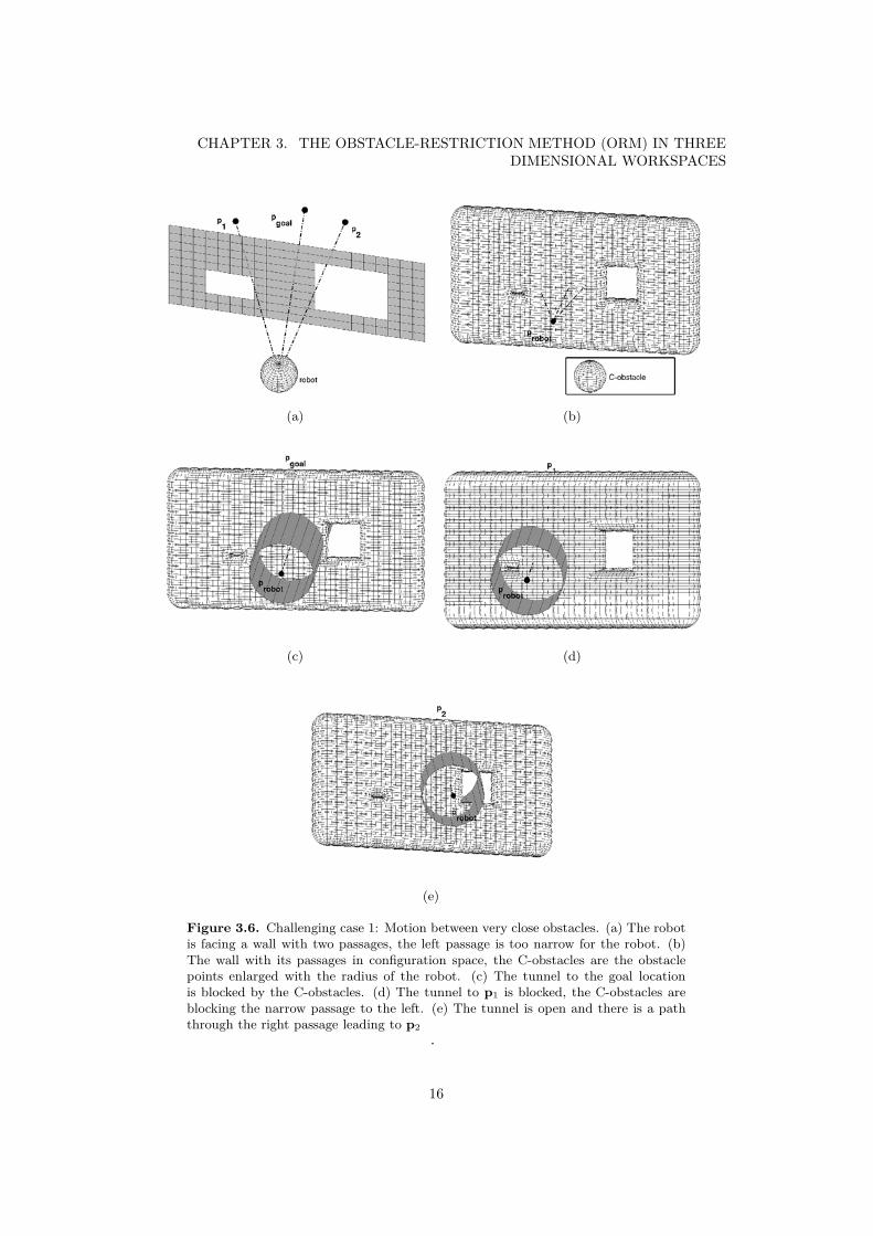
Figure 3.6. Challenging case 1: Motion between very close obstacles. (a) The robotis facing a wall with two passages, the left passage is too narrow for the robot. (b)The wall with its passages in configuration space, the C-obstacles are the obstaclepoints enlarged with the radius of the robot. (c) The tunnel to the goal locationis blocked by the C-obstacles. (d) The tunnel to p1 is blocked, the C-obstacles areblocking the narrow passage to the left. (e) The tunnel is open and there is a paththrough the right passage leading to p2

.

16


(a) (b)

(c) (d)

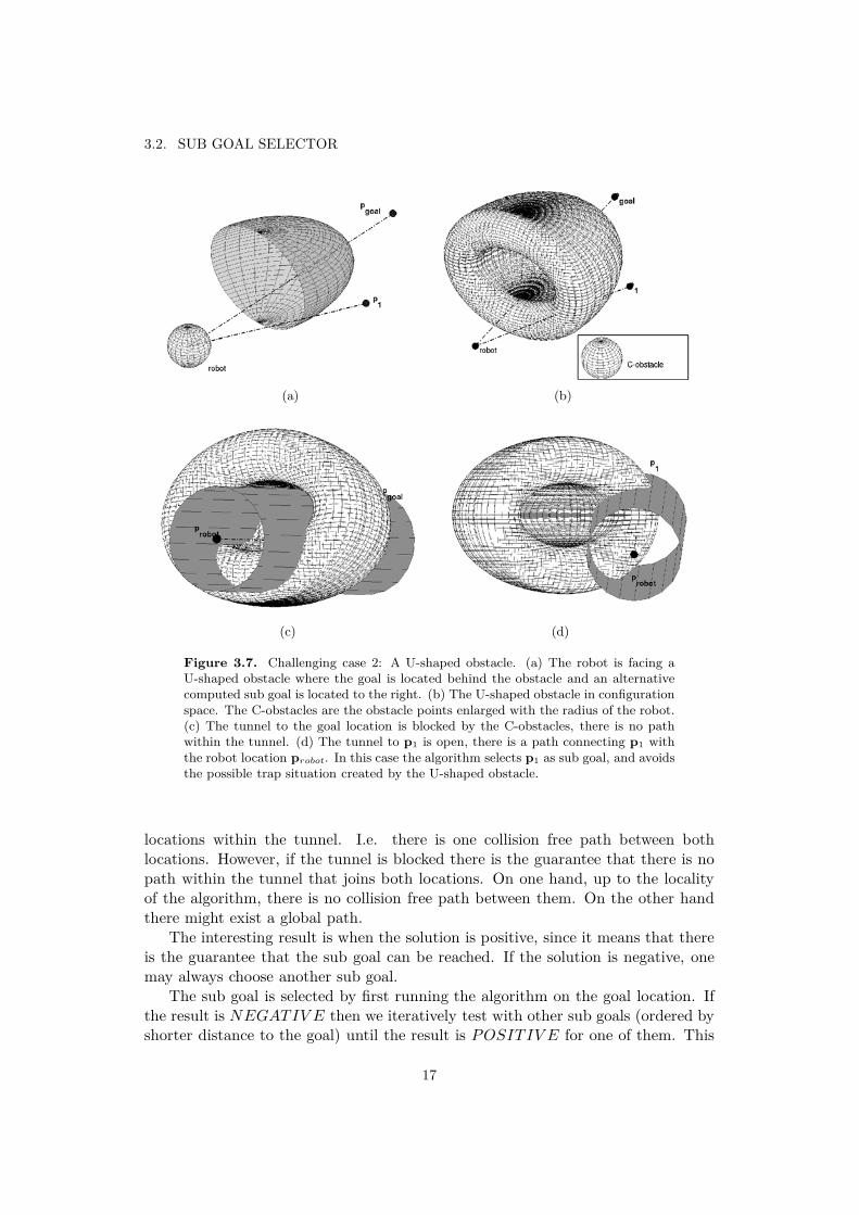
Figure 3.7. Challenging case 2: A U-shaped obstacle. (a) The robot is facing aU-shaped obstacle where the goal is located behind the obstacle and an alternativecomputed sub goal is located to the right. (b) The U-shaped obstacle in configurationspace. The C-obstacles are the obstacle points enlarged with the radius of the robot.(c) The tunnel to the goal location is blocked by the C-obstacles, there is no pathwithin the tunnel. (d) The tunnel to p1 is open, there is a path connecting p1 withthe robot location probot. In this case the algorithm selects p1 as sub goal, and avoidsthe possible trap situation created by the U-shaped obstacle.

locations within the tunnel. I.e. there is one collision free path between bothlocations. However, if the tunnel is blocked there is the guarantee that there is nopath within the tunnel that joins both locations. On one hand, up to the localityof the algorithm, there is no collision free path between them. On the other handthere might exist a global path.

The interesting result is when the solution is positive, since it means that thereis the guarantee that the sub goal can be reached. If the solution is negative, onemay always choose another sub goal.

The sub goal is selected by first running the algorithm on the goal location. Ifthe result is NEGATIV E then we iteratively test with other sub goals (ordered byshorter distance to the goal) until the result is POSITIV E for one of them. This

17


sub goal is selected for motion. For example, in figure (3.6) the algorithm returnsNEGATIV E when tried with pgoal and p1, while the result is POSITIV E whentried with p2.

Many of the obstacle avoidance methods have situations that cause local minima(the trap situation mentioned in the introduction). Next we describe how the subgoal algorithm selects sub goals that direct the motion in such a way that thesesituations are avoided:

1. Motion between very close obstacles (figure 3.6). In the wall, there are twopassages and thus, two different ways to reach the goal. The algorithm returnsNEGATIV E for p1 because the robot does not fit in the narrow passageand thus the tunnel is blocked (figure 3.6(d)). But the algorithm returnsPOSITIV E for p2, which means that the robot fits in this passage (figure3.6(e)). Notice that directing the motion towards p2 avoids the trap situationor collision in the narrow passage.

2. The U-shaped obstacle (figure 3.7). The algorithm returns NEGATIV Ewhen it is used on the goal location pgoal (figure 3.7(c)). When it is used onp1 (figure 3.7(d)) it returns POSITIV E and p1 is selected as alternative subgoal where to direct the motion of the robot. Notice that when choosing p1 assub goal, the robot avoids entering the U-shaped obstacle, and thus the trapsituation is avoided.

Notice that this algorithm is used in combination with a procedure that locatesthe sub goals in the space to capture the structure of the scenario.

3.3 Motion Computation

The sub goal algorithm in the previous section selects a location in the space whereto direct the motion of the robot. This location, the goal or a computed sub goal,is from now on referred to as the target. This section introduces the space divisionthat will be used in the next subsections. Then, we discuss the motion computationthat has two steps: First a set of motion constraints for each obstacle is computed,second, all sets are managed in order to compute the most promising direction ofmotion.

Let the frame of reference from now on be the robot frame, where the origin isp0 = (0, 0, 0), the unitary vectors of the axes (ex, ey, ez) where ex is aligned withthe main direction of motion of the vehicle.

3.3.1 Portions of the Space (subspaces)

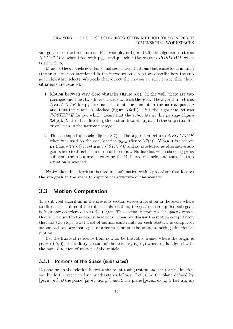
Depending on the relation between the robot configuration and the target directionwe divide the space in four quadrants as follows. Let A be the plane defined by[p0, ex, ez ], B the plane [p0, ez,utarget], and C the plane [p0, ey,utarget]. Let nA, nB

18

3.3. MOTION COMPUTATION

(a) (b)

(c) (d)

(e)

Figure 3.8. Shows step by step how the space is divided into four subspaces. (a)Plane A with normal nA divides the space into the left hand side and the right handside of the robot. (b) Plane B with normal nB divide the space into the left side andthe right side of the target. (c) Plane C with normal nC divide the space into the topside and the down side of the target. (d) Plane A and plane B creates together leftside and right side. (e) Plane C divide left side and right side into the four subspaces:top-left, down-left, top-right and down-right.

19


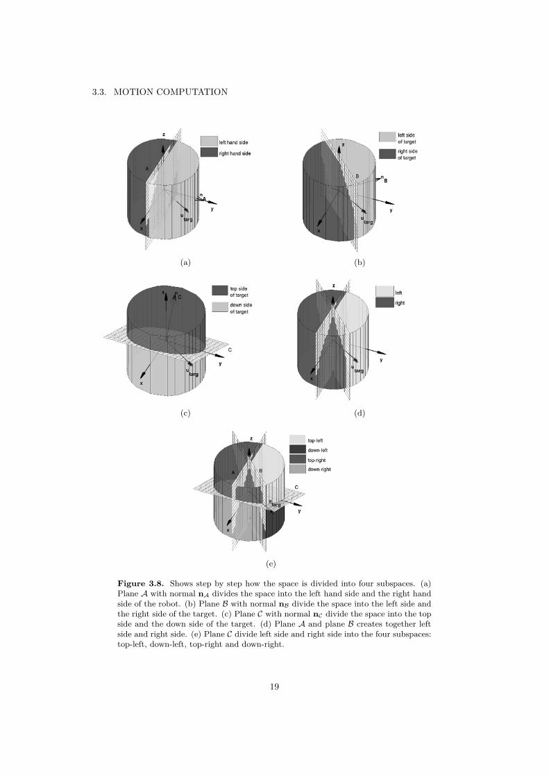
and nC be the normals to these planes respectively, computed by:

nA = ey (3.1)nB = ez ⊗ utarg (3.2)nC = utarg ⊗ ey (3.3)

Then, let u be a given vector, the quadrants are computed by:⎛⎜⎜⎝

TL if (u · nA ≥ 0)& (u · nB ≥ 0)& (u · nC ≥ 0)TR if ((u · nA < 0) | (u · nB < 0))& (u · nC ≥ 0)DL if (u · nA ≥ 0)& (u · nB ≥ 0)& (u · nC < 0)DR if ((u · nA < 0) | (u · nB < 0))& (u · nC < 0)

⎞⎟⎟⎠ (3.4)

where TL, TR, DL and DR are Top-Left, Top-Right, Down-Left, Down-Right re-spectively. Figure 3.8 shows an example.

3.3.2 The motion constraintsThis section describes the computation of a motion constraint for a given obstacle.A motion constraint includes a set of directions SnD ∈ R

3 that are not desired formotion. This set is computed as the union of two subsets S1 and S2. S1 representsthe side of the obstacle, which is not suitable for avoidance, while S2 is an exclusionarea around the obstacle. The first subset of directions S1 is created by the threeplanes described next.

Let uobst be the unitary vector in the direction of the obstacle point pobst. LetD be the plane defined by [p0,uobst,utarget ⊗ uobst], where the normal nD is givenby:

nD = (utarg ⊗ uobst) ⊗ uobst (3.5)

We now define three sets of the space A+, B+ and D+. Given a vector v, wecheck if it belongs to any of these sets as follows:⎛

⎜⎜⎜⎜⎝v ∈ A+ iff nA · v ≥ 0 and (pobst ∈ TL or pobst ∈ DL)v ∈ A+ iff nA · v < 0 and (pobst ∈ TR or pobst ∈ DR)v ∈ B+ iff nB · v ≥ 0 and (pobst ∈ TL or pobst ∈ DL)v ∈ B+ iff nB · v < 0 and (pobst ∈ TR or pobst ∈ DR)v ∈ D+ if nD · v > 0

⎞⎟⎟⎟⎟⎠ (3.6)

where the expression to compute if a direction belongs to a given subspace (TL,DL, TR, DR) is given by expression (3.4). Figure 3.9 and 3.10 shows examples.

Then the motion constraint S1 is computed by:

S1 =

{(A+ ∩ B+) ∩ D+ if pobst ∈ TL or pobst ∈ DL(A+ ∪ B+) ∩ D+ if pobst ∈ TR or pobst ∈ DR

(3.7)

where the expression (3.4) computes whether a point belongs to a given subspace.For example the first case is depicted in figure 3.9 and the second one in figure 3.10.

20


(a) (b)

(c) (d)

(e) (f)

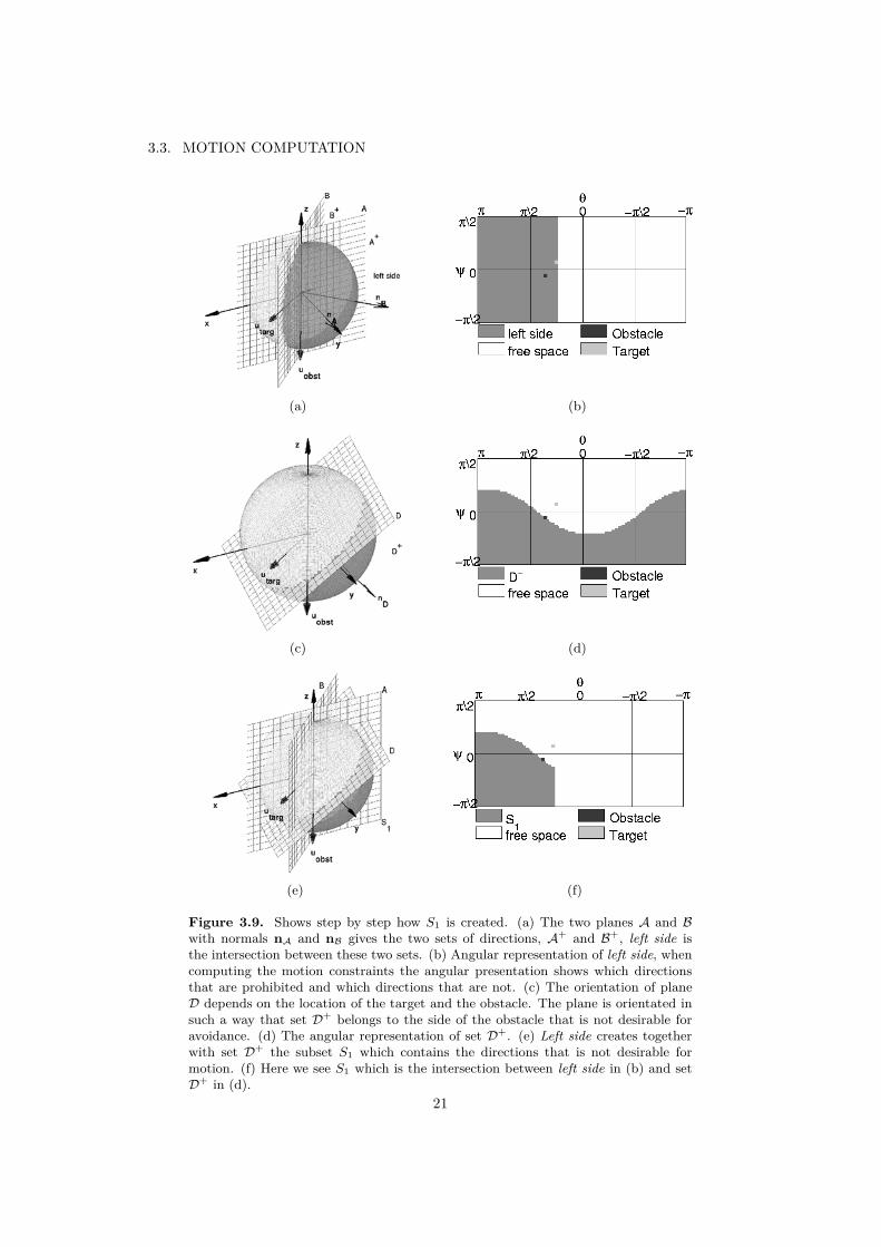
Figure 3.9. Shows step by step how S1 is created. (a) The two planes A and Bwith normals nA and nB gives the two sets of directions, A+ and B+, left side isthe intersection between these two sets. (b) Angular representation of left side, whencomputing the motion constraints the angular presentation shows which directionsthat are prohibited and which directions that are not. (c) The orientation of planeD depends on the location of the target and the obstacle. The plane is orientated insuch a way that set D+ belongs to the side of the obstacle that is not desirable foravoidance. (d) The angular representation of set D+. (e) Left side creates togetherwith set D+ the subset S1 which contains the directions that is not desirable formotion. (f) Here we see S1 which is the intersection between left side in (b) and setD+ in (d).

21


(a) (b)

(c) (d)

(e) (f)

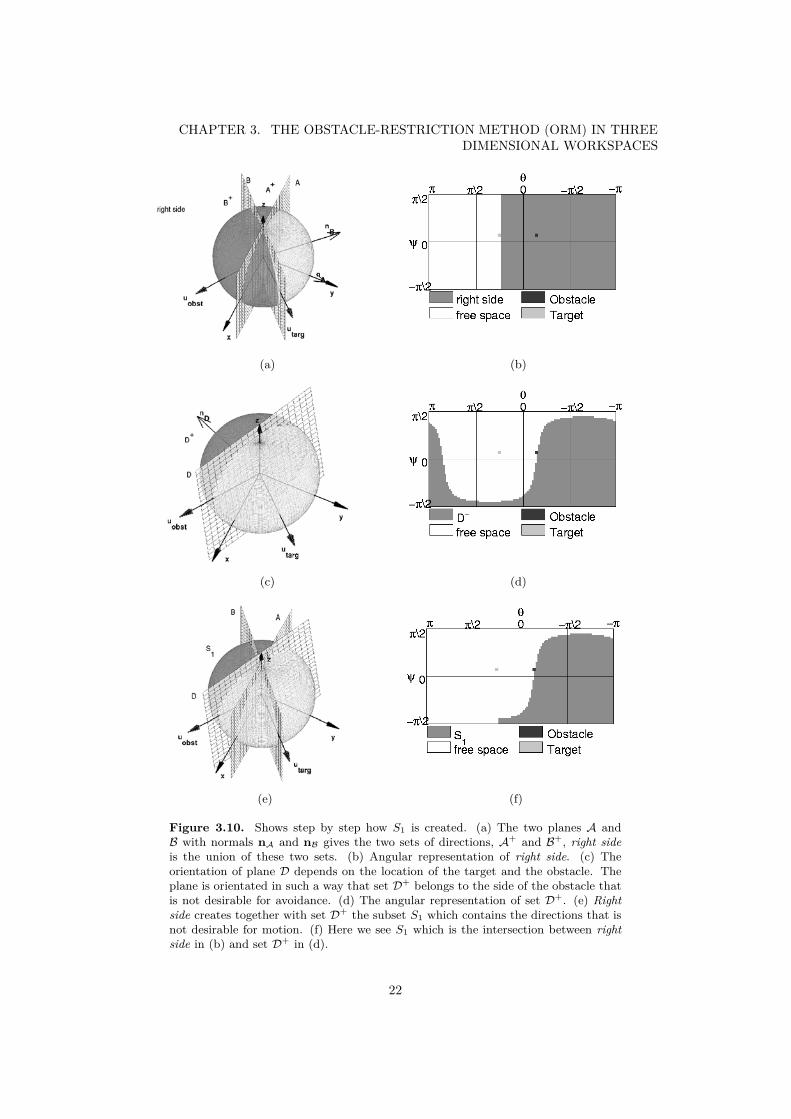
Figure 3.10. Shows step by step how S1 is created. (a) The two planes A andB with normals nA and nB gives the two sets of directions, A+ and B+, right sideis the union of these two sets. (b) Angular representation of right side. (c) Theorientation of plane D depends on the location of the target and the obstacle. Theplane is orientated in such a way that set D+ belongs to the side of the obstacle thatis not desirable for avoidance. (d) The angular representation of set D+. (e) Rightside creates together with set D+ the subset S1 which contains the directions that isnot desirable for motion. (f) Here we see S1 which is the intersection between rightside in (b) and set D+ in (d).

22


The second subset of directions S2 is an exclusion area around the obstacle. LetR be the radius of the robot, Ds a security distance around the robot’s bounds anddobst = ‖pobst‖ the distance to the obstacle. We define S2 as follows:

S2 = {ui | γi ≤ γ} (3.8)

whereγi = arccos

(ui · uobst

‖ui‖ · ‖uobst‖)

(3.9)

andγ = α+ β , 0 < γ < π (3.10)

where α and β is given by,

α = |atan(R+Ds

dobst

)| (3.11)

β =

{(π − α)

(1 − dobst−R

Ds

)if dobst ≤ Ds +R,

0 otherwise(3.12)

Figure 3.11 shows an example. The subset S2 is a cone with the radius R +Ds atthe height of the obstacle. The surface of the cone is the boundary to the subset S2.Moving in any direction of this boundary will remove the obstacle from the robot’ssecurity zone at the height of the obstacle.

The angle is γ = α when the distance to the obstacle is greater than the securitydistance plus the robot’s radius (Figures 3.11(b)–(c)). When the obstacle is withinthe robot’s security zone a term β is added and γ = α + β (Figure 3.11(d)–(e)).The angle γ ranges from 0 to π depending on the distance to the obstacle (γ = 0where the dobst → ∞ and thus there is no deviation, and γ = π when dobst → Rand thus the exclusion area is maximized). Notice that in order to have continuityβ = 0 when the distance to the obstacle is Ds + R (transition limit in expression(3.12)).

Finally, the motion constraint (SnD, set of not desirable directions of motion)for the obstacle is the union of the two subsets: SnD = S1 ∪ S2, Figure 3.12 showsan example.

A feature that will be used latter is the concept of the boundary Sbound to SnD.Let us denote S2−bound the boundary to S2 (i.e. all directions ui such as γi = γ).We define Sbound as:

Sbound = {ui ∈ SnD | ui ∈ S2−bound and ui /∈ S1} (3.13)

In other words, Sbound is the part of the boundary to S2 that does not belong tothe subset S1 (see Figure 3.12). When moving in a direction of this boundary, therobot avoids the obstacle on the desired side while, at the same time, selecting oneof the shorter directions to reach the target.

23


(a)

(b)

θπ π\2 0 −π\2 −π

ψ

π\2

0

−π\2S

2S

2−boundsfree space

ObstacleTarget

(c)

(d)

θπ π\2 0 −π\2 −π

ψ

π\2

0

−π\2S

2S

2−boundsfree space

ObstacleTarget

(e)

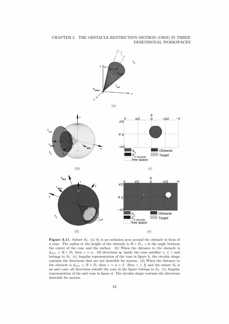
Figure 3.11. Subset S2. (a) S2 is an exclusion area around the obstacle in form ofa cone. The radius at the height of the obstacle is R + Ds, γ is the angle betweenthe center of the cone and the surface. (b) When the distance to the obstacle isdobst > R + Ds then γ = α. All directions ui inside the cone satisfies γi ≤ γ andbelongs to S2. (c) Angular representation of the cone in figure b, the circular shapecontains the directions that are not desirable for motion. (d) When the distance tothe obstacle is dobst < R + Ds then γ = α + β. Here γ > π

2and the subset S2 is

an anti cone, all directions outside the cone in the figure belongs to S2. (e) Angularrepresentation of the anti cone in figure d. The circular shape contains the directionsdesirable for motion.

24


(a)

θπ π\2 0 −π\2 −π

ψ

π\2

0

−π\2S

1S

2S

1 ∩ S

2

Sbound

TargetObstaclesFree space

(b)

(c)

θπ π\2 0 −π\2 −π

ψ

π\2

0

−π\2S

1S

2S

1 ∩ S

2

Sbound

TargetObstaclesFree space

(d)

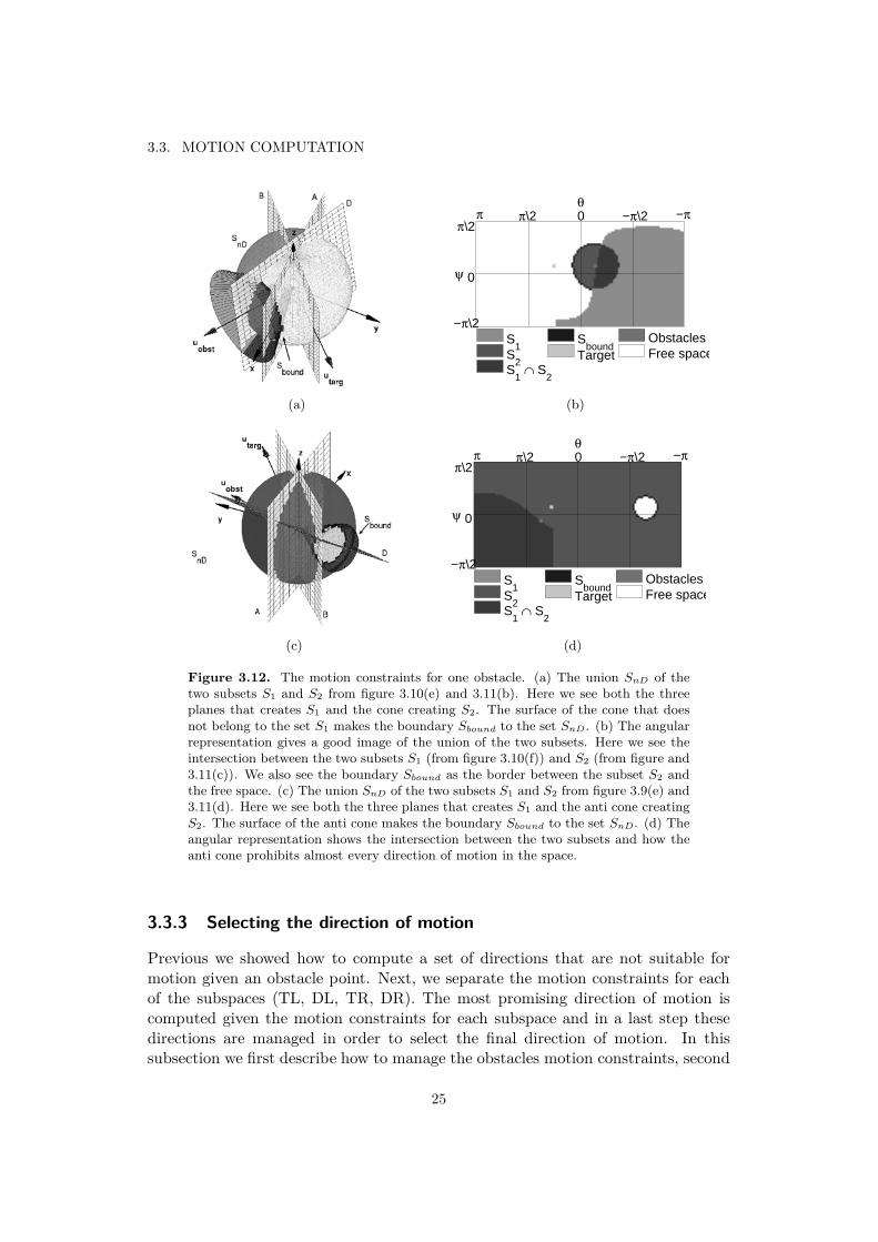
Figure 3.12. The motion constraints for one obstacle. (a) The union SnD of thetwo subsets S1 and S2 from figure 3.10(e) and 3.11(b). Here we see both the threeplanes that creates S1 and the cone creating S2. The surface of the cone that doesnot belong to the set S1 makes the boundary Sbound to the set SnD. (b) The angularrepresentation gives a good image of the union of the two subsets. Here we see theintersection between the two subsets S1 (from figure 3.10(f)) and S2 (from figure and3.11(c)). We also see the boundary Sbound as the border between the subset S2 andthe free space. (c) The union SnD of the two subsets S1 and S2 from figure 3.9(e) and3.11(d). Here we see both the three planes that creates S1 and the anti cone creatingS2. The surface of the anti cone makes the boundary Sbound to the set SnD. (d) Theangular representation shows the intersection between the two subsets and how theanti cone prohibits almost every direction of motion in the space.

3.3.3 Selecting the direction of motion

Previous we showed how to compute a set of directions that are not suitable formotion given an obstacle point. Next, we separate the motion constraints for eachof the subspaces (TL, DL, TR, DR). The most promising direction of motion iscomputed given the motion constraints for each subspace and in a last step thesedirections are managed in order to select the final direction of motion. In thissubsection we first describe how to manage the obstacles motion constraints, second

25


we show how to compute the most promising direction of motion for one subspace,and third how to compute the final direction of motion.

In order to compute the full set of motion constraints we first have to computethe motion constraints for each subspace, and then join them together. For eachobstacle pi in subspace G, we compute the union as:

SG,inD = Si

1 ∪ Si2 (3.14)

then the set of motion constraints for subspace G (e.g. the top-left subspace infigure 3.13) can be written:

SGnD = ∪iSG,i

nD (3.15)

Doing this for each obstacle group gives the four sets STLnD , SDL

nD , STRnD and SDR

nD . Byjoining these four sets together (see example in figure 3.18(b)) we get the full set ofmotion constraints:

SnD = STLnD ∪ SDL

nD ∪ STRnD ∪ SDR

nD (3.16)

SnD contains the directions that are not desired for motion, thus the set of desireddirections is:

SD ={R

3 \ SnD

}(3.17)

We call v a free direction when v ∈ SD. Then we will say that there are freedirections where SD /∈ ∅.

We next describe how to compute the most promising motion direction for eachsubspace. To compute the most promising direction of motion uG

dom for subspacewith SG

nD, we first have to compute the boundary (figure 3.13(b)–(e)). Let SG2−bound

be the boundary to ∪iSi2 for all obstacles pi in obstacle group G, then the boundary

SGbound can be written:

SGbound =

{ui ∈ SnD | ui ∈ SG

2−bound and ui /∈ Si1

}(3.18)

Moving in any direction along this boundary makes sure that all obstacles in Gwill be kept at a distance equal to or greater then the robot’s security distance,at the same time, as one of the shorter directions to reach the target is selected.Therefore when we select uG

dom we choose between the directions in the boundarySG

bound. There are two cases depending on the set of desired directions:

1. There are no free directions, SD ∈ ∅. uGdom is the direction in the boundary

which has the minimum angle to the robot’s current direction of motion, i.e.the x-axis. Let uG

i be all directions in SGbounds and let γi be the angle between

uGi and ex. Let γmin = min(γi) and let uG

min be the direction vector withangle γmin, then:

uGdom = uG

min (3.19)

In this case the robot navigates among close obstacles. Therefore, as smallchanges as possible in the direction of motion is wanted.

26


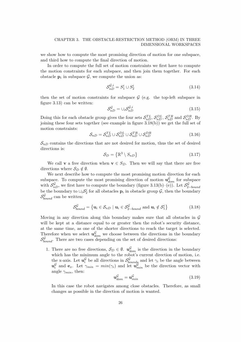
y

obstacles

z

xudom

target

(a) (b)

θπ π\2 0 −π\2 −π

ψ

π\2

0

−π\2S

1S

2S

1∩S

2

Sbound

udom

ObstaclesTargetFree space

(c)

θπ π\2 0 −π\2 −π

ψ

π\2

0

−π\2S

1S

2S

1∩S

2

Sbound

udom


(d)

θπ π\2 0 −π\2 −π

ψ

π\2

0

−π\2S

1S

2S

1∩S

2

Sbound

udom


top left (TL)

(e)

Figure 3.13. Joining the sets. (a) A scenario where the robot is facing two obstaclesthat both belongs to the top-left subspace and creates the top-left motion constraint.(b) This figure shows how the top-left subspace is computed in relation with theconstraints for each obstacle. (c) The angular representation of the set of motionconstraints created by the obstacle located to the left. (d) Angular representationof the set created by the obstacle that is located in above the robot. (e) This figureshows the top-left motion constraint STL

nD which is the union of the two sets in (c)and (d). The boundary Sbounds and the most promising direction of motion udom tothe set is seen in this figure. Notice that the target direction is a free direction, thusthe direction of motion and the target direction is the same.

27


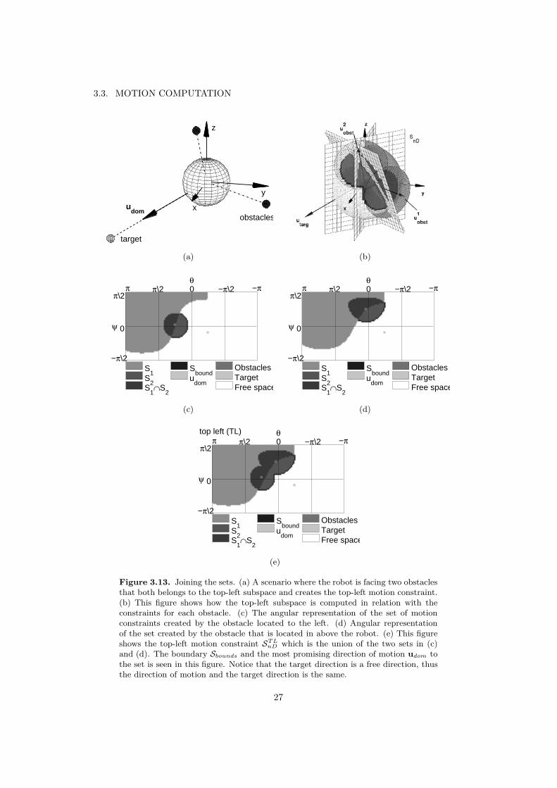
(a)

θπ π\2 0 −π\2 −π

ψ

π\2

0

−π\2S

1S

2S

1∩S

2

Sbound

udom

TargetFree space

SnDTR

(b)

Figure 3.14. Case 2: (a) shows a scenario with obstacles in the the top-rightsubspace. In (b) we see the top-right set of motion constraints which also is the fullset since there are no other obstacles. The target direction belongs to this set andtherefore the most promising direction of motion usol is selected from the directionsin the boundary Sbounds. Free directions exist and thus the direction in the boundaryclosest to the target direction is selected.

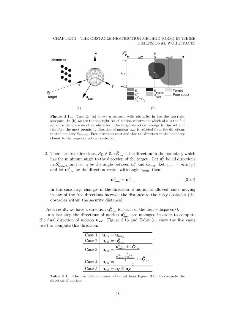
2. There are free directions, SD /∈ ∅. uGdom is the direction in the boundary which

has the minimum angle to the direction of the target . Let uGi be all directions

in SGbounds and let γi be the angle between uG

i and utarg. Let γmin = min(γi)and let uG

min be the direction vector with angle γmin, then:

uGdom = uG

min (3.20)

In this case large changes in the direction of motion is allowed, since movingin any of the free directions increase the distance to the risky obstacles (theobstacles within the security distance).

As a result, we have a direction uGdom for each of the four subspaces G.

In a last step the directions of motion uGdom are managed in order to compute

the final direction of motion usol. Figure 3.15 and Table 3.1 show the five casesused to compute this direction.

Case 1 usol = utarg

Case 2 usol = uGdom

Case 3 usol =uG1

dom + uG2dom

2

Case 4 usol =uG1dom+u

G2dom

2 + uG3dom

2Case 5 usol = nE ⊗ nF

Table 3.1. The five different cases, obtained from Figure 3.15, to compute thedirection of motion.

28


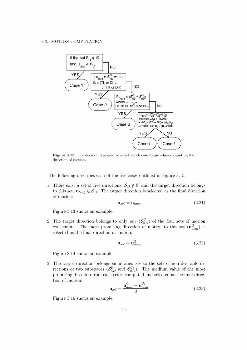
Figure 3.15. The decision tree used to select which case to use when computing thedirection of motion.

The following describes each of the five cases outlined in Figure 3.15.

1. There exist a set of free directions, SD /∈ ∅, and the target direction belongsto this set, utarg ∈ SD. The target direction is selected as the final directionof motion:

usol = utarg (3.21)

Figure 3.13 shows an example.

2. The target direction belongs to only one (SGnD) of the four sets of motion

constraints. The most promising direction of motion to this set (uGdom) is

selected as the final direction of motion:

usol = uGdom (3.22)


3. The target direction belongs simultaneously to the sets of non desirable di-rections of two subspaces (SG1

nD and SG2nD). The medium value of the most

promising direction from each set is computed and selected as the final direc-tion of motion:

usol =uG1

dom + uG2dom

2(3.23)


29


(a)

θπ π\2 0 −π\2 −π

ψ

π\2

0

−π\2

∪S1

∪S2

∩S2

usol

Target

Free space

SnD

(b)

θπ π\2 0 −π\2 −π

ψ

π\2

0

−π\2S

1S

2S

1∩S

2

Sbound

udomDL

TargetFree space

SnDDL

(c)

θπ π\2 0 −π\2 −π

ψ

π\2

0

−π\2S

1S

2S

1∩S

2

Sbound

udomDR

TargetFree space

SnDDR

(d)

Figure 3.16. Case 3: In (a) we have a scenario with obstacles in the the down-leftand the down-right subspaces. There is a space between the two groups of obstacleswhere the robot does not fit, the target is located above and beyond this space. Wealso see the direction of motion from the two sets of motion constraints and themedium value between them usol. The angular representation of the down-left setof motion constraints is seen in (c), here we see the boundary to the set and thedirection of motion uDL

dom. (d) shows the same as in (c) but for the down-right motionconstraints. In (b) we see the full set of motion constraints SnD and the direction ofmotion usol. Notice that the motion is directed higher then the target direction inorder for the robot to avoid the obstacles.

4. The target direction belongs simultaneously to the sets of non desirable motiondirections of three subspaces (SG1

nD, SG2nD and SG3

nD). First the medium value ofthe most promising direction from the two anti symmetric sets (the two antisymmetric sets are either TL–DR or TR–DL) is computed:

uG1−G2dom =

uG1dom + uG2

dom

2(3.24)

Then, the medium value of this direction and the most promising directionfrom the remaining set is computed and selected as the final direction of

30


(a)

θπ π\2 0 −π\2 −π

ψ

π\2

0

−π\2S

1S

2S

1∩S

2

Sbound

udomTR

TargetFree space

SnDTR

(b)

θπ π\2 0 −π\2 −π

ψ

π\2

0

−π\2S

1S

2S

1∩S

2

Sbound

udomDL

TargetFree space

SnDDL

(c)

θπ π\2 0 −π\2 −π

ψ

π\2

0

−π\2S

1S

2S

1∩S

2

Sbound

udomDR

TargetFree space

SnDDR

(d)

θπ π\2 0 −π\2 −π

ψ

π\2

0

−π\2

∪S1

∪S2

∩S2

usol

Target

Free space

SnD

(e)

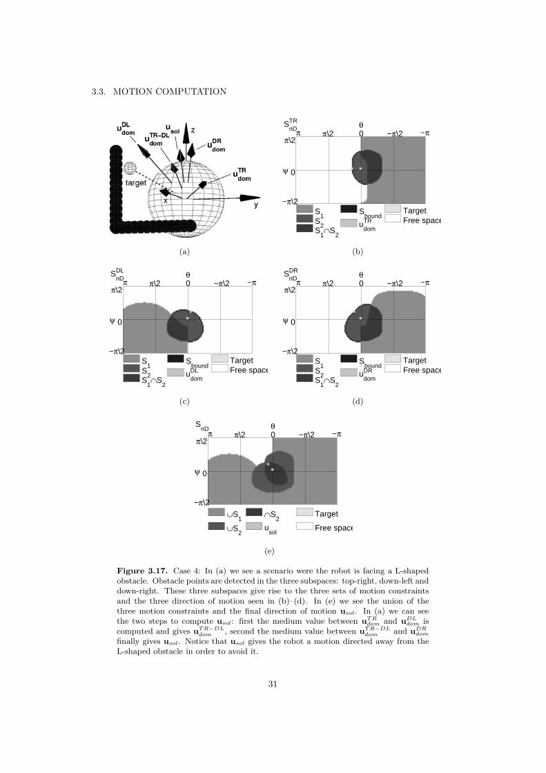
Figure 3.17. Case 4: In (a) we see a scenario were the robot is facing a L-shapedobstacle. Obstacle points are detected in the three subspaces: top-right, down-left anddown-right. These three subspaces give rise to the three sets of motion constraintsand the three direction of motion seen in (b)–(d). In (e) we see the union of thethree motion constraints and the final direction of motion usol. In (a) we can seethe two steps to compute usol: first the medium value between uTR

dom and uDLdom is

computed and gives uTR−DLdom , second the medium value between uTR−DL

dom and uDRdom

finally gives usol. Notice that usol gives the robot a motion directed away from theL-shaped obstacle in order to avoid it.

31


(a)

θπ π\2 0 −π\2 −π

ψ

π\2

0

−π\2

∪S1

∪S2

∩S2

usol

Target

Free space

SnD

(b)

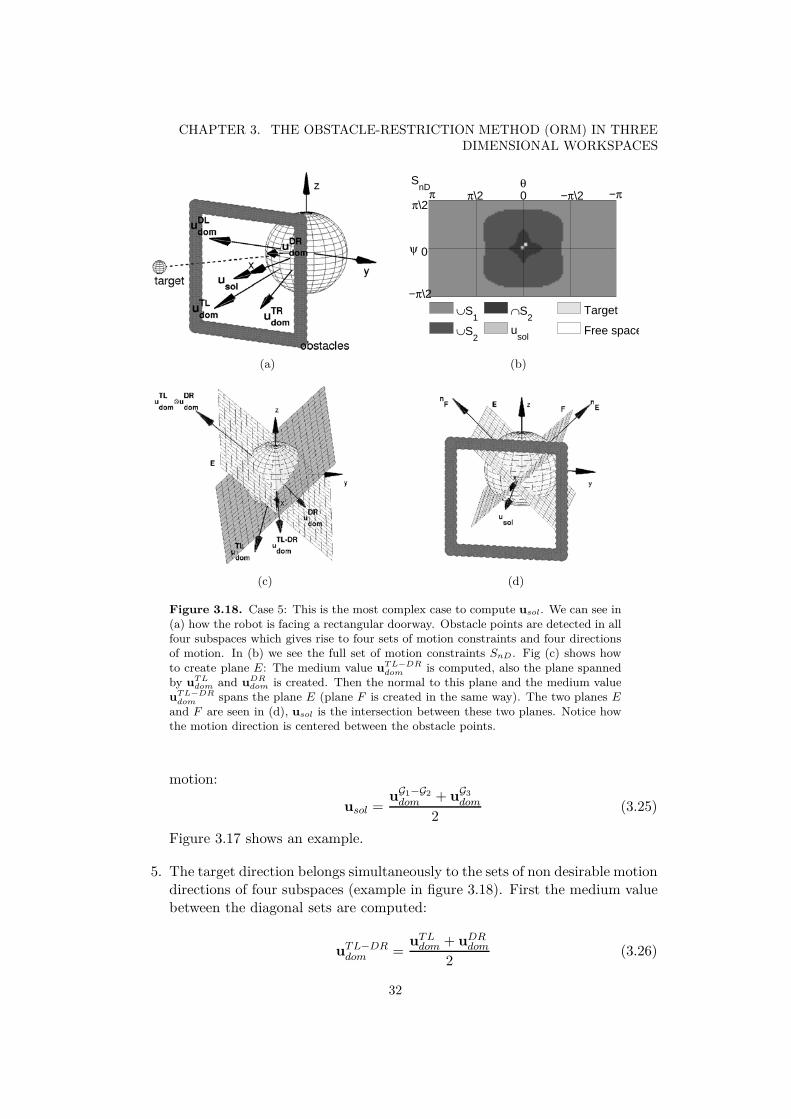
(c) (d)

Figure 3.18. Case 5: This is the most complex case to compute usol. We can see in(a) how the robot is facing a rectangular doorway. Obstacle points are detected in allfour subspaces which gives rise to four sets of motion constraints and four directionsof motion. In (b) we see the full set of motion constraints SnD. Fig (c) shows howto create plane E: The medium value uTL−DR

dom is computed, also the plane spannedby uTL

dom and uDRdom is created. Then the normal to this plane and the medium value

uTL−DRdom spans the plane E (plane F is created in the same way). The two planes E

and F are seen in (d), usol is the intersection between these two planes. Notice howthe motion direction is centered between the obstacle points.

motion:

usol =uG1−G2

dom + uG3dom

2(3.25)


5. The target direction belongs simultaneously to the sets of non desirable motiondirections of four subspaces (example in figure 3.18). First the medium valuebetween the diagonal sets are computed:

uTL−DRdom =

uTLdom + uDR

dom

2(3.26)

32

3.4. COMPUTING THE ROBOT MOTION

uTR−DLdom =

uTRdom + uDL

dom

2(3.27)

Let plane E and F be the planes defined by [p0,uTL−DRdom ,uTL

dom ⊗ uDRdom] and

[p0,uTR−DLdom ,uTR

dom ⊗ uDLdom] respectively. The normals nE and nF are:

nE = (uTLdom ⊗ uDR

dom) ⊗ uTL−DRdom (3.28)

nF = (uTRdom ⊗ uDL

dom) ⊗ uTR−DLdom (3.29)

Moving along the plane E will make the robot centered between the two setsof motion constraints TL and DR. In the same way the robot will be centeredbetween TR and DL when moving along plane F . Therefore, moving along theintersection between these two planes will give the robot a direction of motionwhich keep the robot centered between the four sets of motion constraints.The direction along the intersection between the two planes is selected as thefinal motion of direction:

usol = nE ⊗ nF (3.30)As a result we are able to obtain a promising direction of motion usol in every

situation.

3.4 Computing the Robot MotionIn the previous section the most promising direction of motion usol was determined.This section will show how to compute the motion command that will be given tothe robot. The motion command contains two velocities, the translational velocityυ and the rotational velocity ω. Let us recall that the robot is assumed to beholonomic.

Translational velocity (υ): Let υmax be the maximum translational velocity, dobs

be the distance to the closest obstacle and let Ds be the robot’s securitydistance, then the module of translational velocity:

υ =

⎧⎨⎩υmax ∗ (

π2−|θ|π2

) if dobs > Ds,

υmax ∗ dobsDs

∗ (π2−|θ|π2

) if dobs ≤ Ds.(3.31)

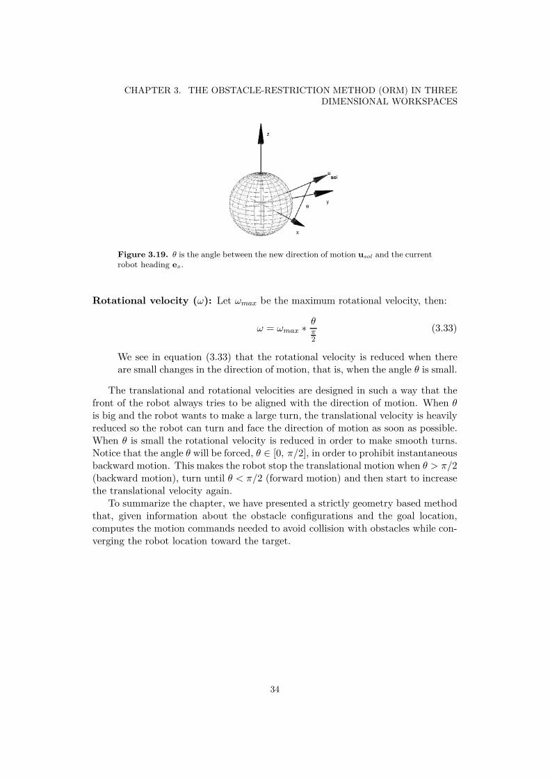
where θ is the angle between the new direction of motion usol and the currentrobot direction of motion, i.e. the x-axis ex (see figure 3.19):

θ = arccos(

usol · ex

‖usol‖ · ‖ex‖)

(3.32)

From equation (3.31) we see that the translational velocity will be reduced ifan obstacle shows up within the security distance. This velocity will also bereduced if there are large changes in the direction of motion, that is, when θis large.

33


Figure 3.19. θ is the angle between the new direction of motion usol and the currentrobot heading ex.

Rotational velocity (ω): Let ωmax be the maximum rotational velocity, then:

ω = ωmax ∗ θπ2

(3.33)

We see in equation (3.33) that the rotational velocity is reduced when thereare small changes in the direction of motion, that is, when the angle θ is small.

The translational and rotational velocities are designed in such a way that thefront of the robot always tries to be aligned with the direction of motion. When θis big and the robot wants to make a large turn, the translational velocity is heavilyreduced so the robot can turn and face the direction of motion as soon as possible.When θ is small the rotational velocity is reduced in order to make smooth turns.Notice that the angle θ will be forced, θ ∈ [0, π/2], in order to prohibit instantaneousbackward motion. This makes the robot stop the translational motion when θ > π/2(backward motion), turn until θ < π/2 (forward motion) and then start to increasethe translational velocity again.

To summarize the chapter, we have presented a strictly geometry based methodthat, given information about the obstacle configurations and the goal location,computes the motion commands needed to avoid collision with obstacles while con-verging the robot location toward the target.

34

Chapter 4

Simulation Results

4.1 Simulation SettingsThe extension of ORM was tested in Matlab where the simulation environmentswere created with points. This because usually the sensor information is given inthis form (i.e. laser rangefinders) or other information can be expressed in this form.The robot was assumed to be spherical and holonomic. We added the constraint thatinstant backwards motion was prohibited. This is because usually robots and sensorshave a main direction of motion. The radius of the robot was set to 0.3m and thesecurity distance to 0.6m. The maximum translational velocity was set to 0.3 m

sec andthe maximum rotational velocity to 0.7rad

sec . The velocities, the security distance andthe size of the robot were set to match the parameters in the Obstacle RestrictionMethod [15], where the application is human transportation. The sampling timewas set to 250ms to match the frequency of the 3D laser scanners available today.

4.2 SimulationsThe five simulations presented here were carried out in unknown and unstructuredscenarios. Only the goal location was given in advance. The simulations weredesigned to verify that the extension of the ORM complies with the goal of thisproject: To safely drive a robot in dense, cluttered and complex scenarios. Further-more, these simulations will allow a discussion in Chapter 5 of the advantages ofthis method. The advantages are briefly summarized next:

• Avoiding trap situations due to the perceived environment structure, e.g. U-shaped obstacles and very close obstacles,

• computing stable and oscillation free motion,

• exhibiting a high goal insensitivity, i.e. to be able to choose a direction faraway from the goal direction,

• selecting motion direction towards obstacles.

35

CHAPTER 4. SIMULATION RESULTS

(a) (b)

(c)

0 5 10 15−0.5

0

0.5

TRANSLATIONAL VELOCITY

time (sec)

Vel

ocity

(m

/sec

)

0 5 10 15−0.5

0

0.5

ROTATIONAL VELOCITY θ

time (sec)Vel

ocity

(ra

d/se

c)

0 5 10 15−0.5

0

0.5

ROTATIONAL VELOCITY ψ

time (sec)Vel

ocity

(ra

d/se

c)

(d)

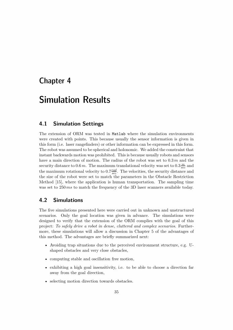
Figure 4.1. Simulation 1. (a) Trajectory of vehicle and scenery. (b),(c) Snapshotsof simulation. (d) Velocity profiles of the simulation.

Simulation 1: Motion in narrow spaces

In this simulation, the robot reached the goal location in a dense scenario withnarrow places, where the space to maneuver was highly reduced (see the scenarioand the robot’s trajectory in figure 4.1(a)). Here the robot managed to enter thenarrow passage (the snapshot in figure 4.1(b)) and travel along it (the snapshotin figure 4.1(c)) with oscillation free motion, which is illustrated in the robot’strajectory and the velocity profiles (the figure 4.1(d)). In the passage the robotmoved among obstacles, distributed all around the robot, to which the distance tothe robot bounds was about 0.2m (the narrow passage had a radius of 0.5m).

The simulation was carried out in 20 sec, and the average translational velocitywas 0.159 m

sec .

Simulation 2: Motion in complex scenario

In this simulation the robot reached the goal location after navigating in a com-plex scenario (see the robot’s trajectory and the scenery in figure 4.2(a)). In some

36

4.2. SIMULATIONS

(a) (b)

(c) (d)

0 5 10 15 20 25 30−0.5

0

0.5


time (sec)

Vel

ocity

(m

/sec

)

0 5 10 15 20 25 30−0.5

0

0.5


time (sec)Vel

ocity

(ra

d/se

c)

0 5 10 15 20 25 30−0.5

0

0.5


time (sec)Vel

ocity

(ra

d/se

c)

(e)

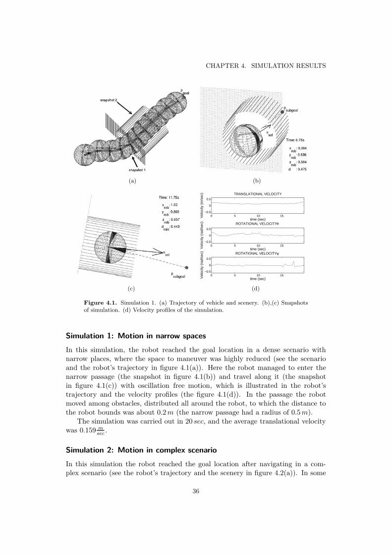
Figure 4.2. Simulation 2. (a) Trajectory of vehicle and scenery. (b)–(d) Snapshotsof simulation. (e) Velocity profiles of the simulation.

parts of the simulation (when passing the doorways) the robot navigated amongclose obstacles (the snapshots in figure 4.2(b) and 4.2(d)). During almost all thesimulation the method had to direct the motion toward obstacles (the snapshotsin figure 4.2(b) and 4.2(c)) in order to converge to the goal location. The method

37


(a) (b)

(c)

0 5 10 15 20−0.5

0

0.5


time (sec)

Vel

ocity

(m

/sec

)

0 5 10 15 20−0.5

0

0.5


time (sec)Vel

ocity

(ra

d/se

c)

0 5 10 15 20−0.5

0

0.5


time (sec)Vel

ocity

(ra

d/se

c)

(d)

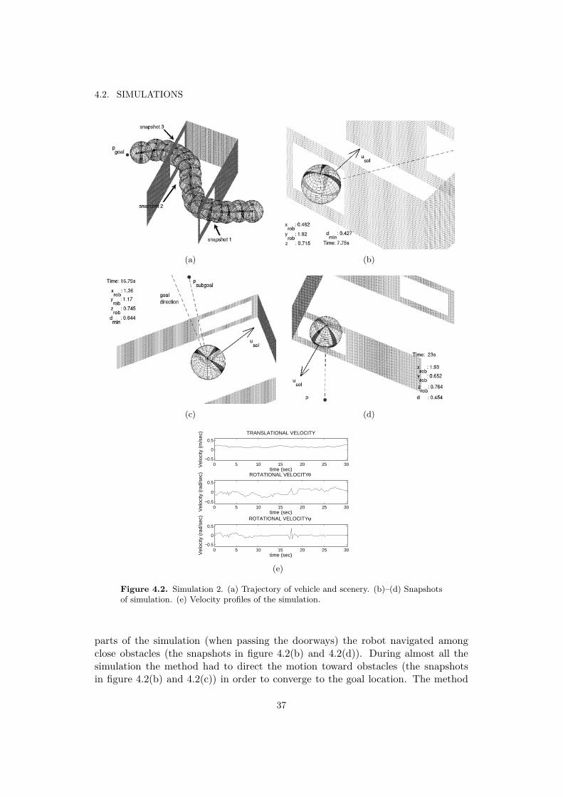
Figure 4.3. Simulation 3. (a) Trajectory of vehicle and scenery. (b),(c) Snapshotsof simulation. (d) Velocity profiles of the simulation.

also selected directions of motions far away from the goal direction (the snapshotin figure 4.2(c)). The velocity profiles is presented in figure (4.2(e)).

The time of the simulation was 30 sec and the average translational velocity was0.153 m

sec .

Simulation 3: Motion avoiding a U-shape obstacle

In this simulation, the robot had to avoid a U-shaped obstacle before it could reachthe goal location (see the trajectory and the scenery in figure 4.3(a)). The methodavoided entering and getting trapped inside the obstacle by directing the motiontoward alternative sub goals that were located on the outside of the U-shapedobstacle (the snapshot in figure 4.3(b)). Motions directed far away from the goaldirection had to be selected (the snapshot in figure 4.3(c)) in order to avoid theU-shaped obstacle. The velocity profiles are presented in figure (4.3(d)).

The time of the simulation was 24 sec, and the average translational velocitywas 0.223 m

sec .

38

4.2. SIMULATIONS

(a) (b)

(c) (d)

0 5 10 15 20 25 30−0.5

0

0.5


time (sec)

Vel

ocity

(m

/sec

)

0 5 10 15 20 25 30−0.5

0

0.5


time (sec)Vel

ocity

(ra

d/se

c)

0 5 10 15 20 25 30−0.5

0

0.5


time (sec)Vel

ocity

(ra

d/se

c)

(e)

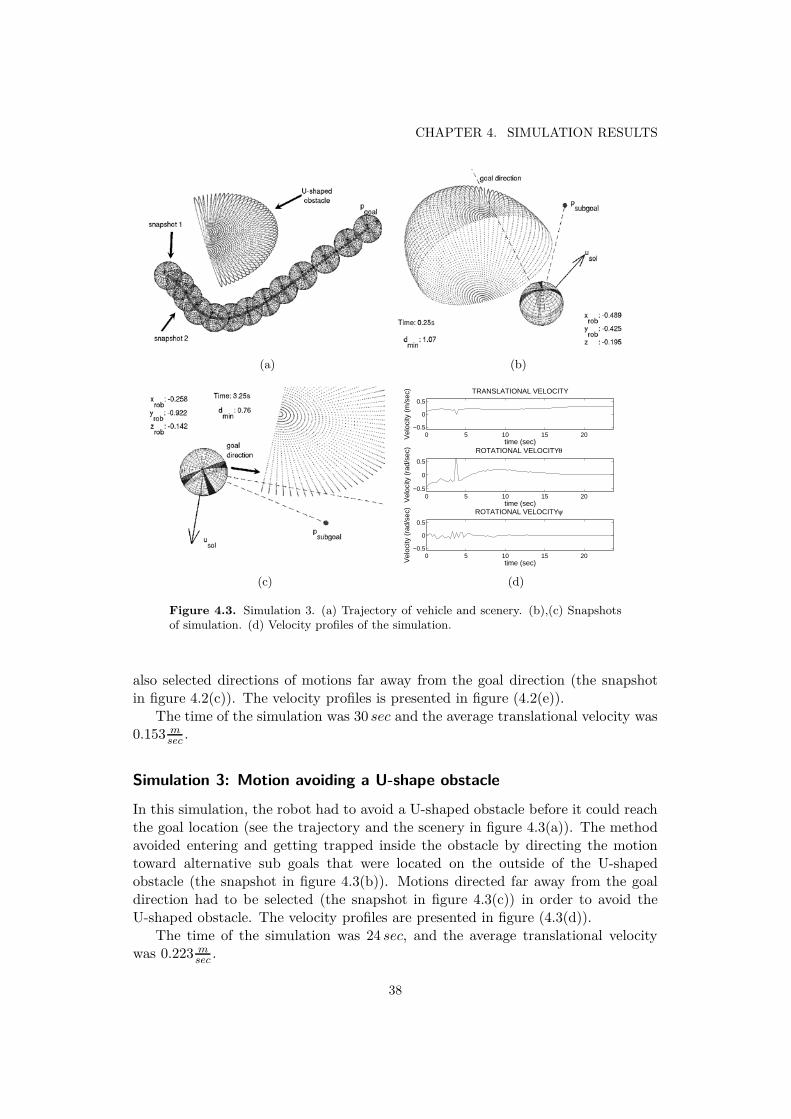
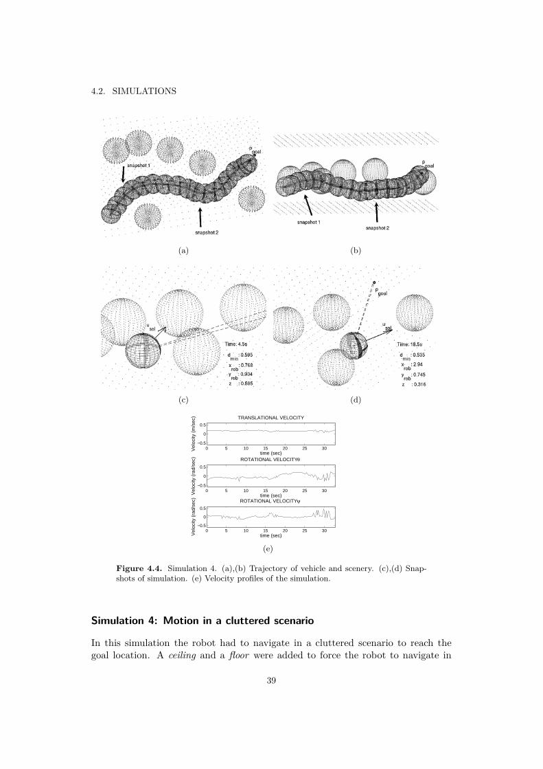
Figure 4.4. Simulation 4. (a),(b) Trajectory of vehicle and scenery. (c),(d) Snap-shots of simulation. (e) Velocity profiles of the simulation.

Simulation 4: Motion in a cluttered scenario

In this simulation the robot had to navigate in a cluttered scenario to reach thegoal location. A ceiling and a floor were added to force the robot to navigate in

39


between the obstacles (see the scenery and the robot trajectory in figure 4.4(a) and4.4(b)). In order to reach the goal the robot had to select motions directed towardthe obstacles (the snapshots in figure 4.4(c) and 4.4(d)) as well as motions directedfar away from the goal direction (the snapshot in figure 4.4(d)). The velocity profilesis presented in figure (4.4(e)).

The simulation was carried out in 33 sec, and the average translational velocitywas 0.162 m

sec .

40

Chapter 5

Discussion

We discuss in this section the advantages of this method with regard to existingtechniques, on the basis of the difficult scenarios shown in the simulation results.Since there is little evidence of obstacle avoidance methods performing in threedimensional workspaces, we assume here that the 3D methods would inherit theproperties of their formulation in 2D.

The local trap situations due to U-shaped obstacles or due to motion amongclose obstacles are overcome with this method. First, the extension of ORM does notdirect the motion within U-shaped obstacles since the sub goal selector places thesub goals outside of these obstacles. However, sometimes while the obstacle is notfully perceived with the sensors, the motion could be directed within an U-shapedobstacle (this is an intrinsic limitation of obstacle avoidance methods). Second, themethod drives the robot among close obstacles because: (i) the sub goal selectorfirst checks whether the robot fits in the narrow passage; (ii) the motion computedcenters the robot among obstacles. This is because, among close obstacles, themotion is obtained as the intersection of the two planes (see Case 5 in section3.3.3) which centers the motion between the four subspaces. In both cases, thePotential Field Methods [10] produce local minima that trap the robot [11]. Alsothe methods based on polar histogram [3], [20], [21] have difficulties navigatingamong close obstacles due to the tuning of an empirical threshold. Traps due to U-shaped obstacle are not avoided by the methods that use constrained optimizations[1], [7], [18], [6]. This occurs because the optimization loses the information of theenvironment structure that is necessary to solve this situation. The methods basedon a given path deformed in real time [9], [17], [5], [4] are trapped when the pathlies within dynamically created U-shaped obstacles.

The extension of ORM has an oscillation free and stable motion whenmoving among close obstacles. This is because information from all obstacles areused to compute the motion, and thus, the difference of the sensor information fromtwo following time cycles is very small. Here the potential field methods can produceoscillatory motion when moving among close obstacles or in narrow corridors [11].

Motion directions far away from the goal direction is obtained with the

41

CHAPTER 5. DISCUSSION

extension of ORM. This is because the sub goals can be placed in any location of thespace, and any direction of the space can be obtained as a solution. The obstacleavoidance methods that makes a physical analogy (e.g. [8], [2], [10], [12], [14] and[19] ) uses the goal location directly in the motion heuristic. The methods thatuse constrained optimizations [6], [18], [7], [1] use the goal direction as one of thebalance terms. Therefore, these methods have high goal sensitivity.

The selection of motions towards the obstacles is obtained by the extensionof ORM. Some methods explicitly prohibit the selection of motion towards obstacles(e.g. [20]).

One difficulty found in almost every obstacle avoidance method is the tuningof internal parameters. The extension of ORM has no internal parameters, onlythe security distance has to be set to a coherent value (in our implementation weset this distance to twice the robot radius).

The presented method overcomes many of the problems and limitations foundin obstacle avoidance methods performing in two dimensional workspaces, whichlead to very good results when driving a vehicle in difficult scenarios. This was theobjective of this experimental validation.

42

Chapter 6

Conclusions

This master’s project addresses obstacle navigation in three dimensional work-spaces. We have presented the design of an obstacle avoidance method that success-fully drives a robot in dense, cluttered and complex environments in three dimen-sional workspaces. The design is an extension of an existing method [15] performingin two dimensions with outstanding results. The proposed method has two steps:First a procedure computes instantaneous sub goals in the obstacle structure; sec-ond a motion restriction is associated with each obstacle which next is managed tocompute the most promising direction of motion.

The advantage with this method is inherited from its precursor: It avoids theproblems and limitations that are common in other obstacle avoidance methods,which leads to very good navigation performance in difficult scenarios.

The disadvantage with this and all the obstacle avoidance methods is that theyare local techniques used to address the motion problem, and thus, the global trapsituations persist (in these cases the robot might never converge to the goal loca-tion). This problem is solved by integrating the obstacle avoidance method witha global motion planning method, but this issue is far beyond the scope of thisproject.

Obstacle avoidance in three dimensions is a very new research area. The maincontribution of this project is the theoretical aspects of obstacle avoidance in difficultthree dimensional workspaces.

43

Bibliography

[1] K. Arras, J. Persson, N. Tomatis, and R. Siegwart. Real-time Obstacle Avoid-ance for Polygonal Robots with a Reduced Dynamic Window. In IEEE Int.Conf. on Robotics and Automation, pages 3050–3055, 2002. Washington, USA.

[2] J. Borenstein and Y. Koren. Real-Time Obstacle Avoidance for Fast MobileRobots. IEEE Transactions on Systems, Man, and Cybernetics, 19(5):1179–1187, 1989.

[3] J. Borenstein and Y. Koren. The Vector Field Histogram - Fast ObstacleAvoidance for Mobile Robots. IEEE Transactions on Robotics and Automation,7(3):278–288, 1991.

[4] O. Brock. Generating Robot Motion: The Integration of Planning and Execu-tion. PhD thesis, Stanford University, 1999. Stanford, CA.

[5] O. Brock and O. Khatib. Real time replanning in high-dimensional configura-tion spaces using sets of homotopic paths. In IEEE Int. Conf. on Robotics andAutomation, pages 550–555, 2000. San Francisco, CA.

[6] W. Feiten, R. Bauer, and G. Lawitzky. Robust Obstacle Avoidance in Unknownand Cramped Environments. In Proc. IEEE Intl. Conference on Robotics andAutomation, pages 2412–2417, 1994. San Diego, CA.

[7] D. Fox, W. Burgard, and S. Thrun. The Dynamic Window Approach to Col-lision Avoidance. In IEEE Robotics & Automation Magazine, volume 4, pages23–33, 1997.

[8] K.Azarm and G.Schmidt. Integrated Mobile Robot Motion Planning and Ex-ecution in Changing Indoor Environments. In Proc. of the IEEE InternationalConference of Intelligent Robots and Systems, pages 298–305, 1994. Munchen,Germany.

[9] M. Khatib. Sensor-based motion control for mobile robots. PhD thesis, LAAS-CNRS, 1996. Tolouse, France.

[10] O. Khatib. Real-Time Obstacle Avoidance for Manipulators and MobileRobots. Int. Journal of Robotics Research, 5:90–98, 1986.

45

BIBLIOGRAPHY

[11] Y. Koren and J. Borenstein. Potential Field Methods and Their Inherent Lim-itations for Mobile Robot Navigation. In Proc. IEEE Int. Conf. Robotics andAutomation, volume 2, pages 1398–1404, 1991. Sacramento, CA.

[12] B. Krogh and C. Thorpe. Integrated Path Planning and Dynamic SteeringControl for Autonomous Vehicles. In Proceedings of the 1986 IEEE Interna-tional Conference on Robotics and Automation, pages 1664–1669, 1986. SanFrancisco, CA.

[13] J.P Laumond and J. Minguez. Motion Planning and Obstacle Avoidance. Hand-book on Robotics, Zaragoza, To appear in 2007.

[14] A. Masoud, S Masoud, and M. Bayoumi. Robot Navigation using a PressureGenerated Mechanical Stress Field, The Biharmonical Potential Approach. InIEEE International Conference on Robotics and Automation, pages 124–127,1994. California, USA.

[15] J. Minguez. The Obstacle Restriction Method for Obstacle Avoidance in Dif-ficult Scenarios. In Proceedings of the Conference on Intelligent Robots andSystems, 2005. Edmonton, Canada.

[16] J. Minguez and L. Montano. Nearness Diagram Navigation (ND): CollisionAvoidance in Troublesome Scenarios. IEEE Transactions on Robotics and Au-tomation, 20(1):45–59, 2004.

[17] S. Quinlan and O. Khatib. Elastic Bands: Connecting Path Planning andControl. In IEEE Int. Conf. on Robotics and Automation, pages 802–807,1993. Atlanta, GA.

[18] R. Simmons. The curvature–velocity method for local obstacle avoidance. InProc. IEEE Intl. Conference on Robotics and Automation, pages 3375–3382,1996. Minneapolis, MN.

[19] R. Tilove. Local obstacle avoidance for mobile robots based on the methodof artificial potentials. In IEEE Int. Conf. Robotics and Automation, pages566–571, 1990. Cincinnati, OH.

[20] I. Ulrich and J. Borenstein. VHF+: Reliable Obstacle Avoidance for FastMobile Robots. In IEEE Int. Conf. Robotics and Automation, pages 1572–1577, 1998.

[21] I. Ulrich and J. Borenstein. VHF*: Local Obstacle Avoidance with Look–Ahead Verification. In Proc. IEEE Int. Conf. Robotics and Automation, pages2505–2511, 2000. San Francisco, CA.

46

Appendix A

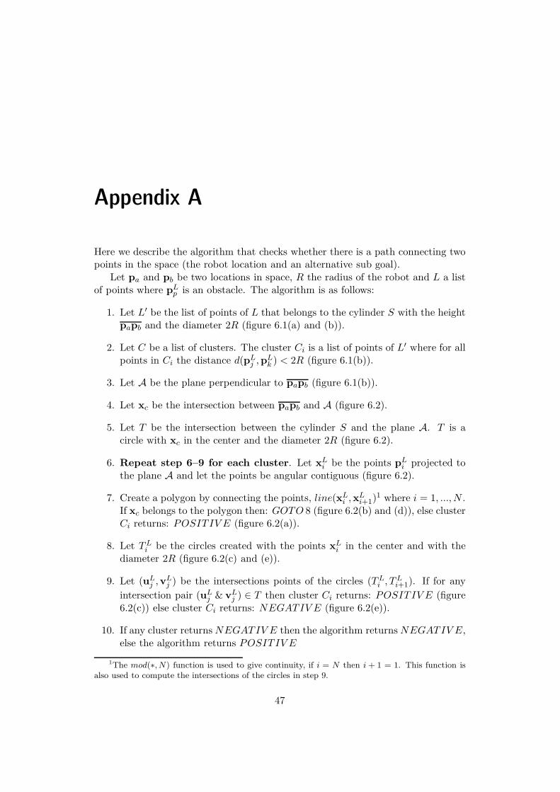
Here we describe the algorithm that checks whether there is a path connecting twopoints in the space (the robot location and an alternative sub goal).

Let pa and pb be two locations in space, R the radius of the robot and L a listof points where pL

p is an obstacle. The algorithm is as follows:

1. Let L′ be the list of points of L that belongs to the cylinder S with the heightpapb and the diameter 2R (figure 6.1(a) and (b)).

2. Let C be a list of clusters. The cluster Ci is a list of points of L′ where for allpoints in Ci the distance d(pL

j ,pLk ) < 2R (figure 6.1(b)).

3. Let A be the plane perpendicular to papb (figure 6.1(b)).

4. Let xc be the intersection between papb and A (figure 6.2).

5. Let T be the intersection between the cylinder S and the plane A. T is acircle with xc in the center and the diameter 2R (figure 6.2).

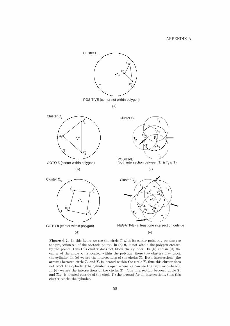
6. Repeat step 6–9 for each cluster. Let xLi be the points pL

i projected tothe plane A and let the points be angular contiguous (figure 6.2).

7. Create a polygon by connecting the points, line(xLi ,x

Li+1)

1 where i = 1, ..., N .If xc belongs to the polygon then: GOTO 8 (figure 6.2(b) and (d)), else clusterCi returns: POSITIV E (figure 6.2(a)).

8. Let TLi be the circles created with the points xL

i in the center and with thediameter 2R (figure 6.2(c) and (e)).

9. Let (uLj ,v

Lj ) be the intersections points of the circles (TL

i , TLi+1). If for any

intersection pair (uLj & vL

j ) ∈ T then cluster Ci returns: POSITIV E (figure6.2(c)) else cluster Ci returns: NEGATIV E (figure 6.2(e)).

10. If any cluster returnsNEGATIV E then the algorithm returnsNEGATIV E,else the algorithm returns POSITIV E

1The mod(∗, N) function is used to give continuity, if i = N then i + 1 = 1. This function isalso used to compute the intersections of the circles in step 9.

47

APPENDIX A

If the algorithm returns:

POSITIV E: there is a local path that connects pa and pb, i.e the final locationcan be reached from the current location.

NEGATIV E: the final location can not be reached within a local area of thespace (the cylinder with radius 2R and height the segment that joins the twolocations). This means that it does not exist a path in this local area of thespace, although there could exist a global one.

48

(a)

(b)

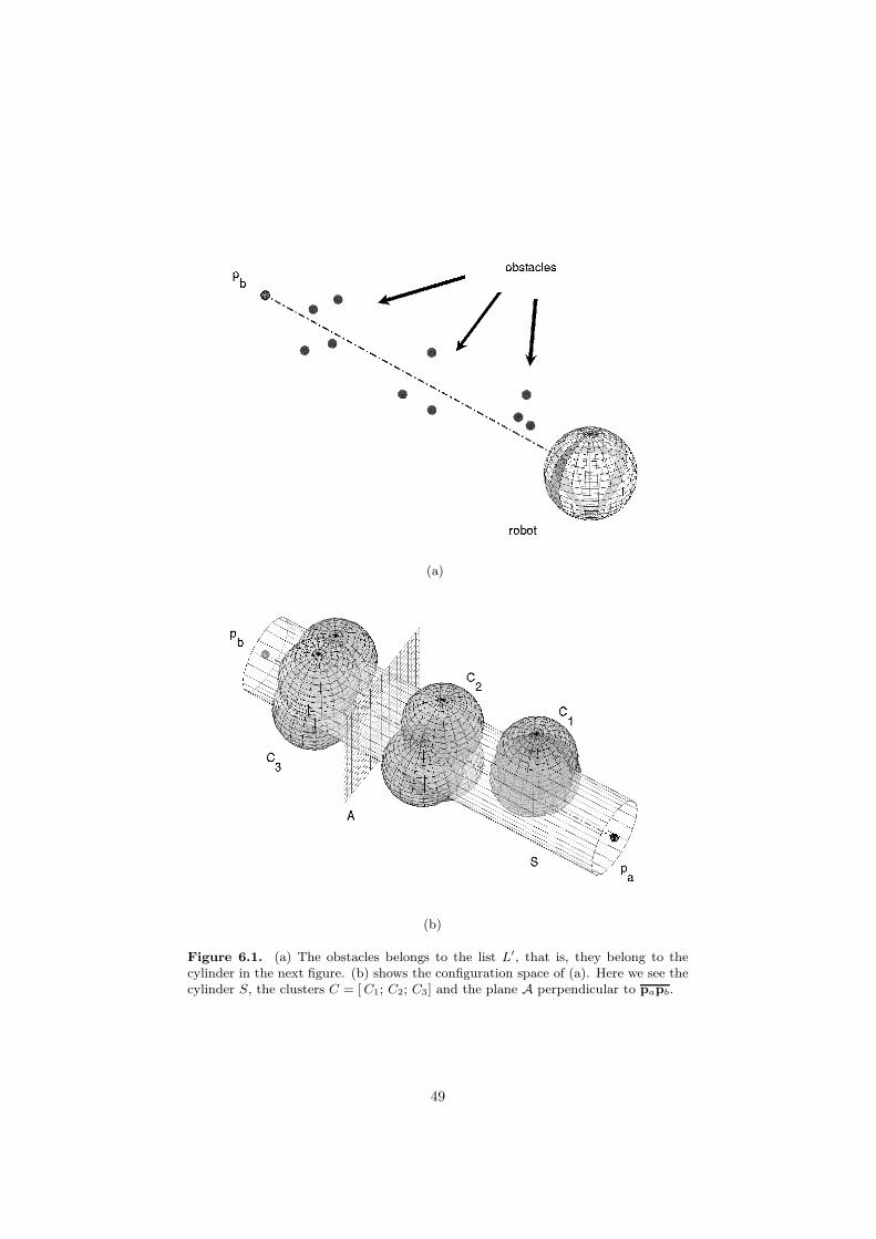
Figure 6.1. (a) The obstacles belongs to the list L′, that is, they belong to thecylinder in the next figure. (b) shows the configuration space of (a). Here we see thecylinder S, the clusters C = [C1; C2; C3] and the plane A perpendicular to papb.

49

APPENDIX A

xc

T

Cluster C1

xL1

xL2

xL3

POSITIVE (center not within polygon)

(a)

xc

T

Cluster C2

xL1

xL2

xL3

GOTO 8 (center within polygon)

(b)

xc

T

Cluster C2

xL1

T1

xL2

T2

xL3

T3

POSITIVE(both intersection between T

1 & T

3 ∈ T)

(c)

xc

T

Cluster C3

xL1

xL2

xL3

xL4

GOTO 8 (center within polygon)

(d)

xc

T

Cluster C3

xL1

T1

xL2

T2

xL3

T3

xL4

T4

NEGATIVE (at least one intersection outside T

(e)

Figure 6.2. In this figure we see the circle T with its center point xc, we also seethe projection xL

i of the obstacle points. In (a) xc is not within the polygon createdby the points, thus this cluster does not block the cylinder. In (b) and in (d) thecenter of the circle xc is located within the polygon, these two clusters may blockthe cylinder. In (c) we see the intersections of the circles Ti. Both intersections (thearrows) between circle T1 and T3 is located within the circle T , thus this cluster doesnot block the cylinder (the cylinder is open where we can see the right arrowhead).In (d) we see the intersections of the circles Ti. One intersection between circle Ti

and Ti+1 is located outside of the circle T (the arrows) for all intersections, thus thiscluster blocks the cylinder.

50

TRITA-CSC-E 2006:172 ISRN-KTH/CSC/E--06/172--SE

ISSN-1653-5715

www.kth.se

the obstacle-restriction method (orm) for reactive … · avoidance in difficult scenarios in...

Documents