using virtual worlds, specifically gta5, to learn...

Using Virtual Worlds, Specifically GTA5, to Learn

Distance to Stop Signs

Artur Filipowicz

Princeton University

229 Sherrerd Hall, Princeton, NJ 08544

T: +01 732-593-9067

Email: [email protected]

corresponding author

Jeremiah Liu



T: +01 202-615-5905


Alain Kornhauser



T: +01 609-258-4657 F: +01 609-258-1563


XXX words + Y figures + Z tables

1

mailto:[email protected]



A. Filipowicz, J. Liu, A. Kornhauser 2

1 ABSTRACT

We examine a machine learning system, convolutional neural network, which mimics hu-

man vision to detect stop signs and estimate the distance to them based on individual images. To

train the network, we develop a method to automatically collect labeled data from Grand Theft

Auto 5. Using this method, we assembled a dataset of 1.4 million images with and without stop

signs across different environments, weather conditions, and times of day. Convolutional neural

network trained and tested on this data can detect 95.5% of the stops signs within 20 meters with

a false positive rate of 5.6% and an average error in distance of 1.2m to 2.4m. We also discovered

that the performance our approach is limited in distance to about 20m. The applicability of these

results to real world driving must be studied further.


2 INTRODUCTION

With increases in automation of the driving task, vehicles are expected to safely navigate

the same roadway environments as human divers. To meet this expectation, future driver assistance

systems and self-driving vehicles require information to determine two fundamental questions of

driving. Those being the location where the vehicle should go next and when it should stop. To

find an answer, a vehicle needs to know its relative position and orientation, not only with respect

to a lane or vehicles, but also with respect to the environment and existing roadway infrastructure.

For example, an autonomous vehicle should be able to recognize the same unaltered stop signs that

are readily recognized by human drivers and slow down and stop, just like human drivers.

In the last decade of autonomous vehicle research, a range of approaches for enabling

vehicles to perceive the environment have emerged depending on the extent to which the existing

roadway infrastructure is augmented from that which exists to serve today’s human drivers and the

amount of historical intelligence that is captured in digital databases and is available in real-time

to the autonomous vehicle system. While humans have recently begun to use turn-by-turn “GPS”

systems that contain historically coded digital map data and freshly captured and processed traffic

and other crowd-sourced intelligence to navigate to destinations, the continuous task of human

driving is accomplished through a purely real-time autonomous approach in which we do not need

any other information from the environment but a picture. In 2005, Princeton University’s entry

in the DARPA Challenge, Prospect 11, followed this idea, using radar and cameras to identify and

locate obstacles. Based on these measurements, the on-board computer would create a world model

and find a safe path within the limits of a desire set of 2D GPS digital map data points (4). Other

projects, such as (27), followed the same approach. Since then the Google Car (14) vastly extended

the use of pre-made digital data by creating, maintaining and distributing pre-made highly detailed

digital 3D maps of existing roadway environments that are then used, in combination with real-

time on-board sensors to locate the vehicle within the existing roadway infrastructure and,

consequently, relative to important stationary elements of that infrastructure such as lanes

markings and stop signs. All of this being accomplished without the need for any augmentation of

the existing roadway infrastructure. Other approaches, motivated by US DoT connected vehicle

research, have proposed the creation of an intelligent infrastructure with electronic elements that

could be readily identified and located by intelligent sensors, thus helping autonomous vehicles

but being of little, if any, direct assistance to existing human drivers (16).

In this paper, we tackle the problem of when the vehicle should stop under the autonomous

approach. More precisely, we examine a machine learning system which mimics human vision to

detect stop signs and estimate the distance to them based purely on individual images. The hope is

that such a system can be designed and trained to perform as well as, if not better, than a human in

real-time while using acceptable computing resources. Importantly, we explore overcoming the

traditional roadblock of training such system: the lack of sufficiently large amounts and variations

of properly labeled training data, by harvesting examples of labeled driving scenes from virtual

environments, in this case, Grand Theft Auto 5 (1; 2; 3).


3 RELATED WORK

In recent years, a wide variety of computer vision and machine learning techniques are

used to achieve high rates of traffic sign detection and recognition. Loy and Barnes use the sym-

metric nature of sign shapes to establish possible shape centroid location in the image and achieve

a detection rate of 95% (22). In (23), the generalization properties of SVMs are used to con- duct

traffic sign detection and recognition. Results show the system is invariant to rotation, scale, and

even to partial occlusion with an accuracy of 93.24%. Another popular technique uses color

thresholding to segment the image and shape analysis to detect signs (9; 21). A neural network is

trained to perform classification on thresholded images obtains an accuracy of around 95% (21; 9).

Lastly, another method employs both single-image and multi-view analysis, where a 97% overall

classification rate is achieved (28).

Research on localization of traffic signs has gained attention more recently. In (19), the

authors describe a real-time traffic sign recognition system along with an algorithm to calculate

the approximate GPS position of traffic signs. There is no evaluation of accuracy regarding the

calculated position. Barth et al. presents a solution for localization of a vehicle’s position and ori-

entation with respect to stop sign controlled intersections based on location specific image features,

GPS, Kalman filtering and map data (5). Based on this method, a vehicle starting 50 m away from

the target intersection can stop within a median distance of 1 cm of the stop line. A panoramic

image-based method for mapping road signs is presented in (15). The method uses mutiple im-

ages for localization and is able to localize 85% of the signs correctly. Accuracy of the calculated

position is not reported.

Similarly, Timofe et al. (28) uses multiple views to locate signs in 3 dimensions with 95%

of the signs located within 3 m of the real location and 90% of signs are located within 50 cm.

Their system uses 8 roof mounted cameras and runs at 2 frames per second. While they do

discuss potential for a real time system running at 16 frames per second, they do not report

localization accuracy (28). Theodosis et al. used a stereo camera for localizing a known size stop

sign by mapping the relative change of pixels to distance. The accuracy of the calculated position

id not discussed in the results (26). Welzel et al. introduced and evaluated two methods for absolute

traffic sign localization using a single color camera and in-vehicle Global Navigation Satellite

System (GNSS). The bearing-based localization approach determines positions of traffic sign

using triangulation on image sequence and the relative localization approach calculates the 3D

position of a traffic sign relative to the host vehicle by calibrating camera matrix and merging with

vehicle position and azimuth obtained from GNSS receiver. (30) The presented algorithms in (30)

are able to provide a reliable traffic sign position with accuracy between 0.2 m and 1.6 m within

the range of 7 m to 25 m from the stop sign.

3.1 Direct Perception

Researchers achieved reasonable accuracy in localization with dependency on additional

sensors such as GNSS or under certain weather and time conditions. We believe that autonomous

driving system can be designed with the camera playing the role of the human eye. For this we

employ direct perception (13) proposed by (8).

Within the autonomous approach to autonomous driving, specific systems can be catego-

rized based on the world model the system constructs. Classical categories include behavior reflex


and mediated perception (29). Behavior reflex (8) approach uses learning models which internal-

ize the world model. Pomerleau used this method to map images directly to steering angles (24).

Mediated perception (9; 7; 29) uses several learning models to detect important features and then

builds a world model based on these features. For example, a mediated perception system would

use a vehicle detector, a pedestrian detector, and a street sign detector to find as many objects as it

can in the driving scene and then estimate the location of all of these objects. As (8) points out,

behavior reflex has difficulties handling complex driving situations while mediated perception often

creates unnecessary complexity in extracting information irrelevant to the driving task.

With considerations of the shortcoming of these approaches, Chen et al. (8) proposed a

direct perception approach. Direct perception creates a model of the world using a few specific

indicators which are extracted directly form the input data. In (8), the computer learns a trans-

formation from images generated in the open source virtual environment TORCS (6), to several

meaningful affordance indicators needed for highway driving. These indicators include distance to

the lane markings and the distances to cars in current and adjacent lanes. Chen et al. showed this

approach works well enough to drive a car in a virtual environment, and generalizes to real images

in the KITTI dataset (12), and to driving on US 1 near Princeton.

4 DEEP LEARNING FOR STOP SIGN RECOGNITION AND LOCAL-

IZATION

Following the direct perception (8; 13) and deep learning (20) paradigms, we construct a

deep convolutional neural network (CNN) (18) and train it to detect and locate stop signs using a

training set of images and ground truths from a video game’s virtual world.

4.1 The Learning Model

Our direct perception convolutional neural network is based on the standard AlexNet archi-

tecture (18) with modifications based on (8). It is built in Caffe (17) and consists of 280 × 210 pixel

input image, 5 convolutional layers followed by 4 fully connected layers with output dimensions

of 4096, 4096, 256, and 2. The two final outputs are a 0/1 indicator which is one when a stop sign

is detected and a continuous distance variable that reflects the estimated distance to the stop sign.

This distance is in the range of 0 to 70 m. If no stop sign is detected, the distance is set to 70 m.

We normalize both outputs to the range of [0.1, 0.9]. The model’s 68.2 million unknown

coefficients are evolved to find the global minimum of the Euclidean loss function using a stochas-

tic gradient decent method with an initial learning rate of 0.01, mini-batches of 64 images, and

300,000 iterations. We call the resulting solution Long Range CNN. We also fine tuned the model

coefficients for short distances by training the final coefficients of Long Range CNN for another

100,000 iterations on examples of stops signs within 40 meters. The output range is redefined to

0.9 representing 40 meters. We refer to this solution as the Short Range CNN.

4.2 Data Collection and Datasets

Large learning models, such as the one we are using, tend to be able to correlate compli-

cated high dimensional input to a small dimensional output given enough data. The rule of thumb


is the larger the model the more data it needs, hence the recent interest in big data. Depending on

the application, collecting large datasets can be very difficult. Often the limiting factor, especially

in datasets of images, is annotating the images with ground truth labels. For our purpose, we would

need a person to indicate if a stop sign is in an image and measure the distance to that stop sign.

This process could be slow and error prone. While a part of this process can be automated by using

measuring tools, such as in (11), this presents additional limitations. Sensors may not function in

all weather conditions, such as rain or fog, and their output may still need to be interpreted by a

human before the desired ground truth is determined. For example lidar measurements will be

noisy during rain and the device outputs a point cloud which a person would need to interpret to

determine the distance to stop sign. We overcome this problem by using a video game called Grand

Theft Auto 5 (GTA5).

Virtual environments have been used by (25) to create a system for construction 3D bound-

ing boxes based on 2D images and (8) to learn distances to road lane markings and cars. For our

application, GTA5 provides a rich road environment from which we can harvest vast amounts of

data. GTA5 has a 259 square kilometers (100 square miles) map (1) with a total population of

4,000,000 people. The game engine populates this world with 262 different types of vehicles (3),

and 1,167 different models of pedestrians and animals. There are 77,934 road segments and 74,530

road nodes (2) which make up a road network of bridges, tunnels, freeways, and intersections in

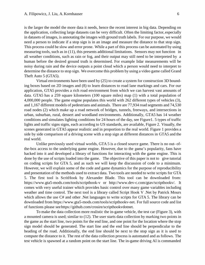
urban, suburban, rural, dessert and woodland environments. Additionally, GTA5 has 14 weather

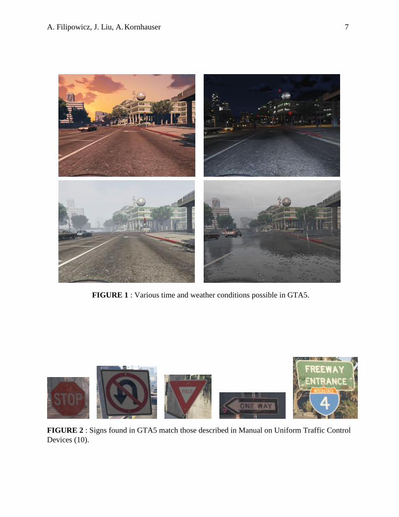
conditions and simulates lighting conditions for 24 hours of the day, see Figure1. 5 types of traffic

lights and traffic signs signs, each according to US standards, are available, Figure 2. Visually, the

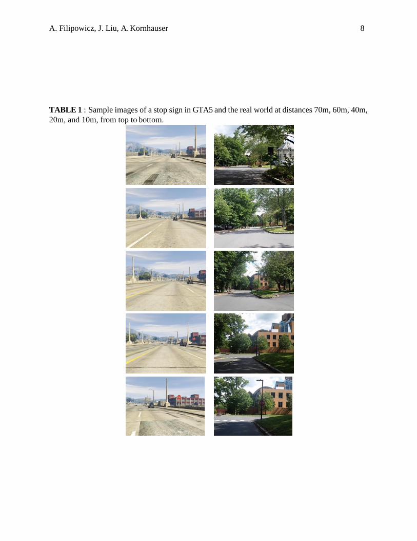
scenes generated in GTA5 appear realistic and in proportion to the real world. Figure 1 provides a

side by side comparison of a driving scene with a stop sign at different distances in GTA5 and the

real world.

Unlike previously used virtual worlds, GTA 5 is a closed source game. There is no out- of-

the-box access to the underlying game engine. However, due to the game’s popularity, fans have

hacked into it and developed a library of functions for interacting with the game engine. This is

done by the use of scripts loaded into the game. The objective of this paper is not to give tutorial

on coding scripts for GTA 5, and as such we will keep the discussion of code to a minimum.

However, we will explain some of the code and game dynamics for the purpose of reproducibility

and presentation of the methods used to extract data. Two tools are needed to write scripts for GTA

5. The first tool is ScritHook by Alexander Blade. This tool can be downloaded from:

https://www.gta5-mods.com/tools/scripthook-v or http://www.dev-c.com/gtav/scripthookv/. It

comes with very useful trainer which provides basic control over many game variables including

weather and time control. The next tool is a library called Script Hook V .Net by Patrick Mours

which allows the use C# and other .Net languages to write scripts for GTA 5. The library can be

downloaded from https://www.gta5-mods.com/tools/scripthookv-net. For full source code and list

of functions please see https://github.com/crosire/scripthookvdotnet.

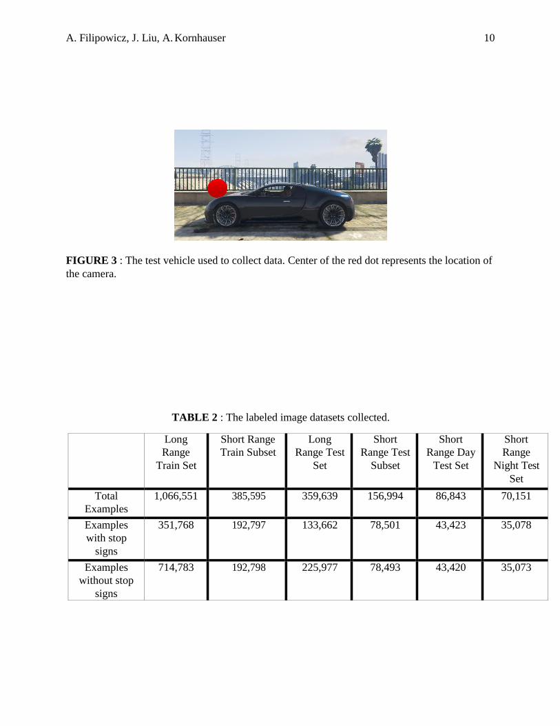
To make the data collection more realistic the in-game vehicle, the test car (Figure 3), with

a mounted camera is used; similar to (12). The user starts data collection by marking two points in

the game as the start line, two points for the end line, and one point for the location where the stop

sign model should be generated. The start line and the end line should be perpendicular to the

heading of the road. Additionally, the end line should be next to the stop sign as it is used to

compute the distance to it. The rest of the data collection process is automated and as follows. The

test vehicle is spawned at a random point on the start line. The in-game driving AI is commanded

http://www.gta5-mods.com/tools/scripthook-v

http://www.dev-c.com/gtav/scripthookv/

http://www.gta5-mods.com/tools/scripthookv-net


FIGURE 1 : Various time and weather conditions possible in GTA5.

FIGURE 2 : Signs found in GTA5 match those described in Manual on Uniform Traffic Control

Devices (10).


TABLE 1 : Sample images of a stop sign in GTA5 and the real world at distances 70m, 60m, 40m,

20m, and 10m, from top to bottom.


to drive the vehicle to a random point on the end line. As the vehicle is driving, pictures of the

game are taken and saved at around 30 frames a second. For each image the ground truth data -

described later - is recorded as well. Once the vehicle reaches the end line, the stop sign model is

turned invisible and the vehicle travels the same route. This helps to create a set of examples with

a clear distinction of what is a stop sign. Once the two passes are made, the hour and weather is

changed and the vehicle is set to travel between another pair of random points. This is repeated for

each of 24 hours and 5 weather conditions; extra sunny, foggy, rain, thunder, and clear. The process

takes about 40 minutes to complete generates about 80,000 properly labeled images.

The ground truth label for each image includes the indicator, the distance, the weather and

the time. The weather, and time are recorded based on the current state of the game. The indicator

is set to 1 if a stop sign is visible in the image, otherwise it is set to 0 and the distance is set to 70m.

When a stop sign is visible, the distance to it is computed as the distance between the center of the

camera’s near clipping plane and the point on the ground next to the stop sign defied by the

intersection of the end line and the heading of the vehicle. While this measure does not take into

account the curvature of the road and thus is not necessarily the road distance to the stop sign, we

chose this measure for three reasons. First, we did not find a way to compute the road distance in

the game. Second, this measure is easier to interpret than the direct distance between the stop sign

and the vehicle. Third, the actual difference in measurement is small. Even in the worst case

scenario, when the stop sign and the road are on the very edge of the field of view, taking our

maximum distance of 70 m and field of view of 60 degrees, the road distance is 60.6 m. In this

situation the vehicle is heading 30 degrees from the heading of the road, and at this angle a standard

lane is only 4.2 meters wide. The discrepancy between the distance does not appear to be of

importance.

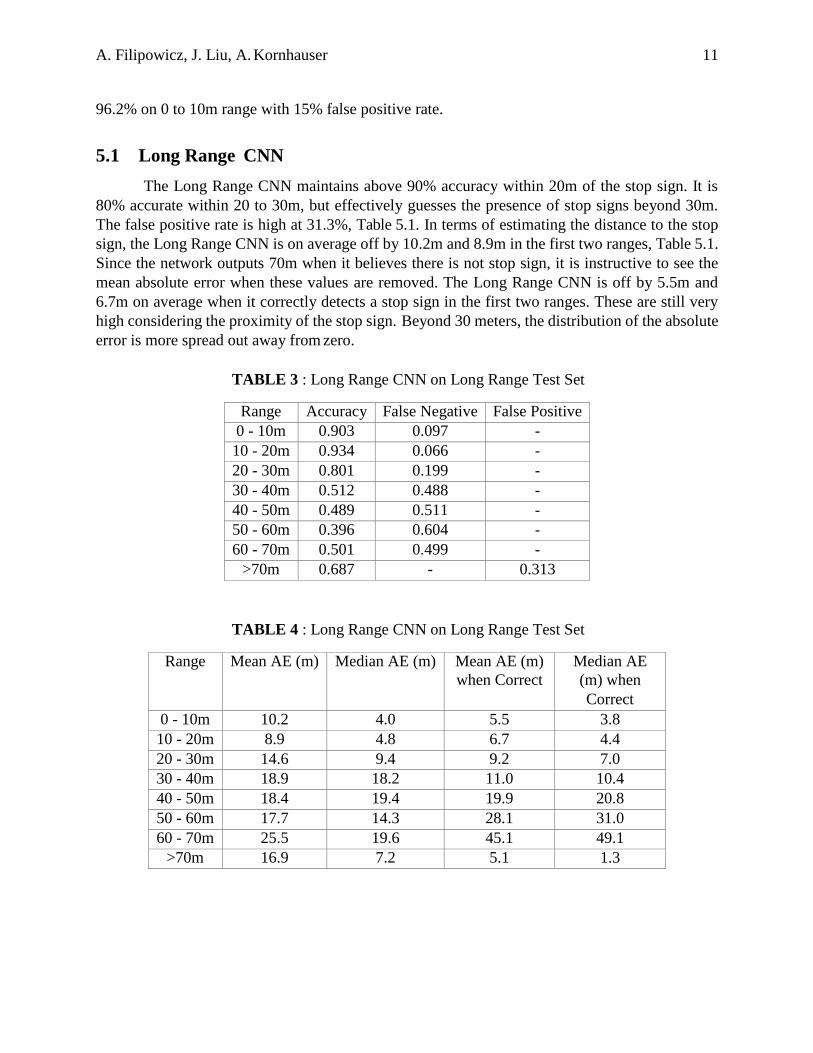
This method collected a total of 1,426,190 images from 25 different locations. We used

over one million images for training and the remainder for testing. Table 4.2 details the number of

images used in the training and test sets. Also created was a data subset for training and testing on

examples of stop signs within 40 meters, as well as subsets for day and night. Training and testing

were performed on completely different locations, and thus the network would be exposed to a

completely new environment. The images are distributed almost uniformly across time and

weather. The total time spent collecting these data was about 10 hours. Collection ceased at 1.4

million images which were used as the basis for quantifying the performance of the Deep Learning

CNN. Table4.2 lists the number of labeled images collected under the various conditions for the

purpose of both training and testing.

5 RESULTS

On GTA5 test examples, The Short Range CNN outperforms the Long Range CNN in both

detection accuracy and absolute error (AE), the absolute value of the difference between the the

network estimated distance and the ground truth distance. It achieves state-of-the-art comparable

accuracy of 96.1% and 94.9% on ranges 0 to 10m and 10 to 20m with an average error in distance

of 2.2m and 3.3m respectively with a 5.6% false positive rate. The performance of both CNNs

degrades substantially beyond 20m, with about a 10% drop in accuracy for range 20 to 30m and

40% drop in accuracy for subsequent ranges. In general, both models perform poorly on our small

real world dataset of 244 images. Although the Short Range CNN did achieve an accuracy of


FIGURE 3 : The test vehicle used to collect data. Center of the red dot represents the location of

the camera.

TABLE 2 : The labeled image datasets collected.

Long

Range

Train Set

Short Range

Train Subset

Long

Range Test

Set

Short

Range Test

Subset

Short

Range Day

Test Set

Short

Range

Night Test

Set

Total

Examples

1,066,551 385,595 359,639 156,994 86,843 70,151

Examples

with stop

signs

351,768 192,797 133,662 78,501 43,423 35,078

Examples

without stop

signs

714,783 192,798 225,977 78,493 43,420 35,073


96.2% on 0 to 10m range with 15% false positive rate.

5.1 Long Range CNN

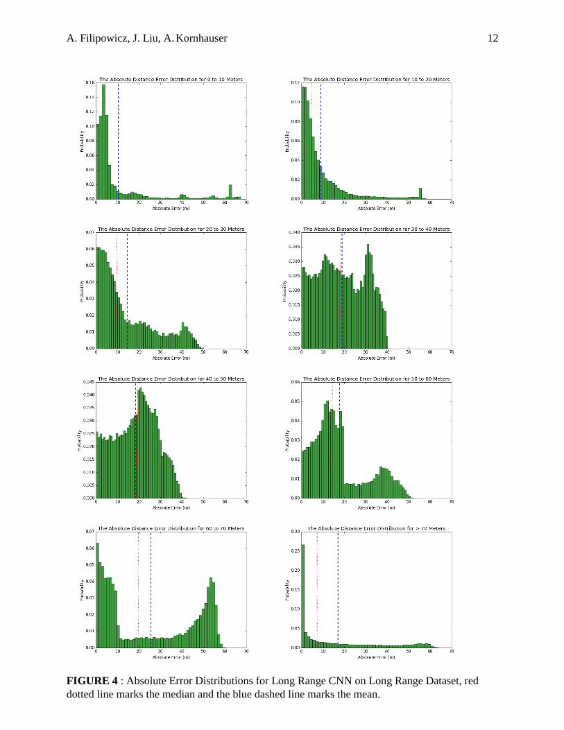
The Long Range CNN maintains above 90% accuracy within 20m of the stop sign. It is

80% accurate within 20 to 30m, but effectively guesses the presence of stop signs beyond 30m.

The false positive rate is high at 31.3%, Table 5.1. In terms of estimating the distance to the stop

sign, the Long Range CNN is on average off by 10.2m and 8.9m in the first two ranges, Table 5.1.

Since the network outputs 70m when it believes there is not stop sign, it is instructive to see the

mean absolute error when these values are removed. The Long Range CNN is off by 5.5m and

6.7m on average when it correctly detects a stop sign in the first two ranges. These are still very

high considering the proximity of the stop sign. Beyond 30 meters, the distribution of the absolute

error is more spread out away from zero.

TABLE 3 : Long Range CNN on Long Range Test Set

Range Accuracy False Negative False Positive

0 - 10m 0.903 0.097 -

10 - 20m 0.934 0.066 -

20 - 30m 0.801 0.199 -

30 - 40m 0.512 0.488 -

40 - 50m 0.489 0.511 -

50 - 60m 0.396 0.604 -

60 - 70m 0.501 0.499 -

>70m 0.687 - 0.313

TABLE 4 : Long Range CNN on Long Range Test Set

Range Mean AE (m) Median AE (m) Mean AE (m)

when Correct

Median AE

(m) when

Correct

0 - 10m 10.2 4.0 5.5 3.8

10 - 20m 8.9 4.8 6.7 4.4

20 - 30m 14.6 9.4 9.2 7.0

30 - 40m 18.9 18.2 11.0 10.4

40 - 50m 18.4 19.4 19.9 20.8

50 - 60m 17.7 14.3 28.1 31.0

60 - 70m 25.5 19.6 45.1 49.1

>70m 16.9 7.2 5.1 1.3


FIGURE 4 : Absolute Error Distributions for Long Range CNN on Long Range Dataset, red

dotted line marks the median and the blue dashed line marks the mean.


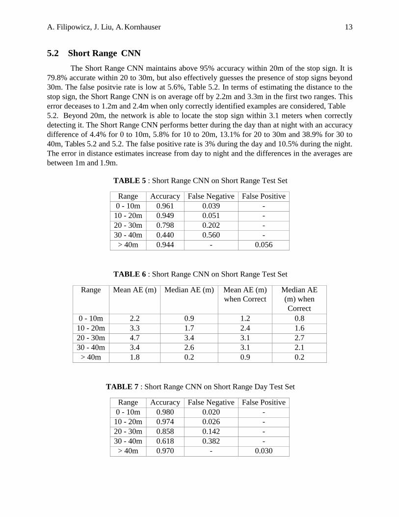
5.2 Short Range CNN

The Short Range CNN maintains above 95% accuracy within 20m of the stop sign. It is

79.8% accurate within 20 to 30m, but also effectively guesses the presence of stop signs beyond

30m. The false positvie rate is low at 5.6%, Table 5.2. In terms of estimating the distance to the

stop sign, the Short Range CNN is on average off by 2.2m and 3.3m in the first two ranges. This

error deceases to 1.2m and 2.4m when only correctly identified examples are considered, Table

5.2. Beyond 20m, the network is able to locate the stop sign within 3.1 meters when correctly

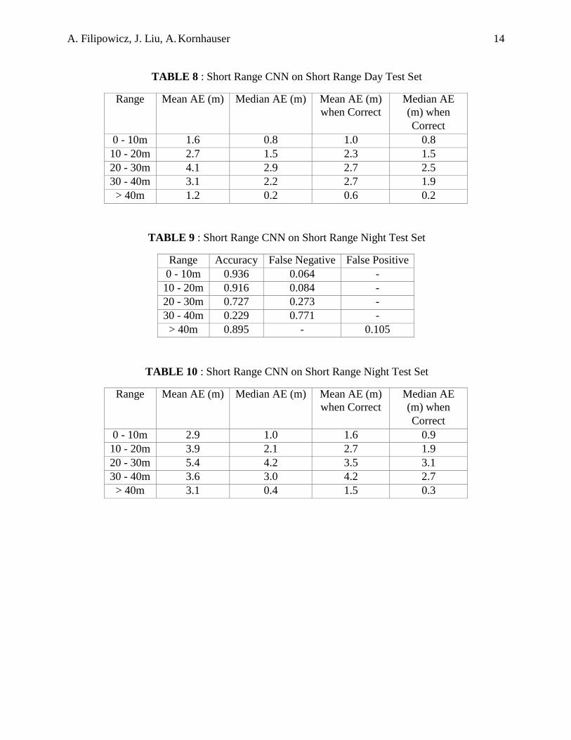
detecting it. The Short Range CNN performs better during the day than at night with an accuracy

difference of 4.4% for 0 to 10m, 5.8% for 10 to 20m, 13.1% for 20 to 30m and 38.9% for 30 to

40m, Tables 5.2 and 5.2. The false positive rate is 3% during the day and 10.5% during the night.

The error in distance estimates increase from day to night and the differences in the averages are

between 1m and 1.9m.

TABLE 5 : Short Range CNN on Short Range Test Set


0 - 10m 0.961 0.039 -

10 - 20m 0.949 0.051 -

20 - 30m 0.798 0.202 -

30 - 40m 0.440 0.560 -

> 40m 0.944 - 0.056

TABLE 6 : Short Range CNN on Short Range Test Set


when Correct

Median AE

(m) when

Correct

0 - 10m 2.2 0.9 1.2 0.8

10 - 20m 3.3 1.7 2.4 1.6

20 - 30m 4.7 3.4 3.1 2.7

30 - 40m 3.4 2.6 3.1 2.1

> 40m 1.8 0.2 0.9 0.2

TABLE 7 : Short Range CNN on Short Range Day Test Set


0 - 10m 0.980 0.020 -

10 - 20m 0.974 0.026 -

20 - 30m 0.858 0.142 -

30 - 40m 0.618 0.382 -

> 40m 0.970 - 0.030


TABLE 8 : Short Range CNN on Short Range Day Test Set


when Correct

Median AE

(m) when

Correct

0 - 10m 1.6 0.8 1.0 0.8

10 - 20m 2.7 1.5 2.3 1.5

20 - 30m 4.1 2.9 2.7 2.5

30 - 40m 3.1 2.2 2.7 1.9

> 40m 1.2 0.2 0.6 0.2

TABLE 9 : Short Range CNN on Short Range Night Test Set


0 - 10m 0.936 0.064 -

10 - 20m 0.916 0.084 -

20 - 30m 0.727 0.273 -

30 - 40m 0.229 0.771 -

> 40m 0.895 - 0.105

TABLE 10 : Short Range CNN on Short Range Night Test Set


when Correct

Median AE

(m) when

Correct

0 - 10m 2.9 1.0 1.6 0.9

10 - 20m 3.9 2.1 2.7 1.9

20 - 30m 5.4 4.2 3.5 3.1

30 - 40m 3.6 3.0 4.2 2.7

> 40m 3.1 0.4 1.5 0.3


FIGURE 5 : Absolute Error Distributions for Short Range CNN on Short Range Test Set, red



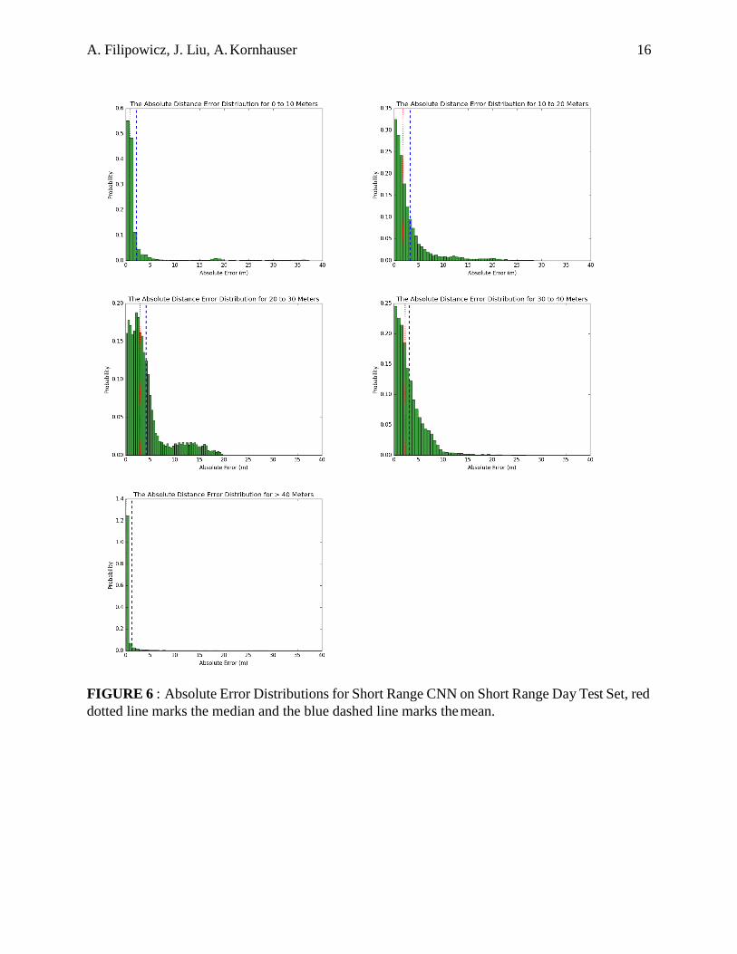
FIGURE 6 : Absolute Error Distributions for Short Range CNN on Short Range Day Test Set, red



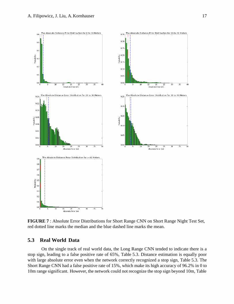
FIGURE 7 : Absolute Error Distributions for Short Range CNN on Short Range Night Test Set,

red dotted line marks the median and the blue dashed line marks the mean.

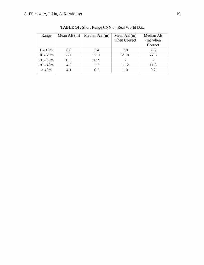
5.3 Real World Data

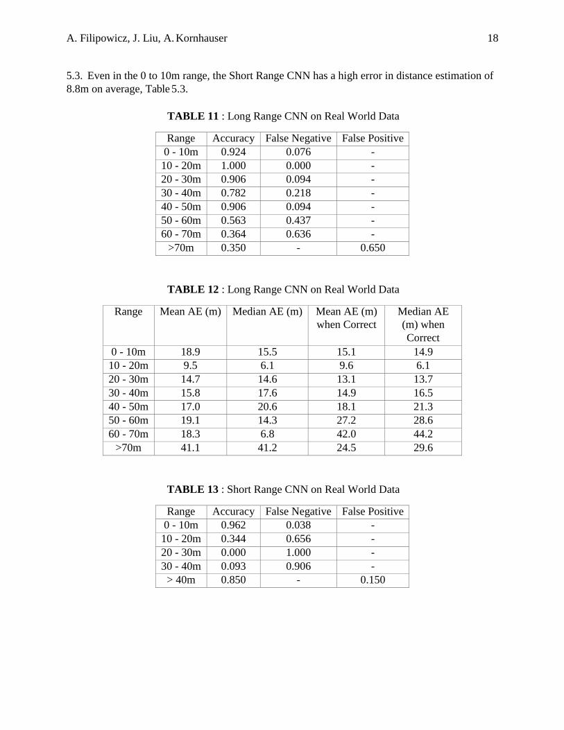
On the single track of real world data, the Long Range CNN tended to indicate there is a

stop sign, leading to a false positive rate of 65%, Table 5.3. Distance estimation is equally poor

with large absolute error even when the network correctly recognized a stop sign, Table 5.3. The

Short Range CNN had a false positive rate of 15%, which make its high accuracy of 96.2% in 0 to

10m range significant. However, the network could not recognize the stop sign beyond 10m, Table


5.3. Even in the 0 to 10m range, the Short Range CNN has a high error in distance estimation of

8.8m on average, Table 5.3.

TABLE 11 : Long Range CNN on Real World Data


0 - 10m 0.924 0.076 -

10 - 20m 1.000 0.000 -

20 - 30m 0.906 0.094 -

30 - 40m 0.782 0.218 -

40 - 50m 0.906 0.094 -

50 - 60m 0.563 0.437 -

60 - 70m 0.364 0.636 -

>70m 0.350 - 0.650

TABLE 12 : Long Range CNN on Real World Data


when Correct

Median AE

(m) when

Correct

0 - 10m 18.9 15.5 15.1 14.9

10 - 20m 9.5 6.1 9.6 6.1

20 - 30m 14.7 14.6 13.1 13.7

30 - 40m 15.8 17.6 14.9 16.5

40 - 50m 17.0 20.6 18.1 21.3

50 - 60m 19.1 14.3 27.2 28.6

60 - 70m 18.3 6.8 42.0 44.2

>70m 41.1 41.2 24.5 29.6

TABLE 13 : Short Range CNN on Real World Data


0 - 10m 0.962 0.038 -

10 - 20m 0.344 0.656 -

20 - 30m 0.000 1.000 -

30 - 40m 0.093 0.906 -

> 40m 0.850 - 0.150


TABLE 14 : Short Range CNN on Real World Data


when Correct

Median AE

(m) when

Correct

0 - 10m 8.8 7.4 7.8 7.3

10 - 20m 22.0 22.1 21.8 22.6

20 - 30m 13.5 12.9 - -

30 - 40m 4.3 2.7 11.2 11.3

> 40m 4.1 0.2 1.0 0.2


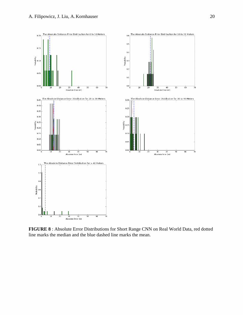
FIGURE 8 : Absolute Error Distributions for Short Range CNN on Real World Data, red dotted

line marks the median and the blue dashed line marks the mean.


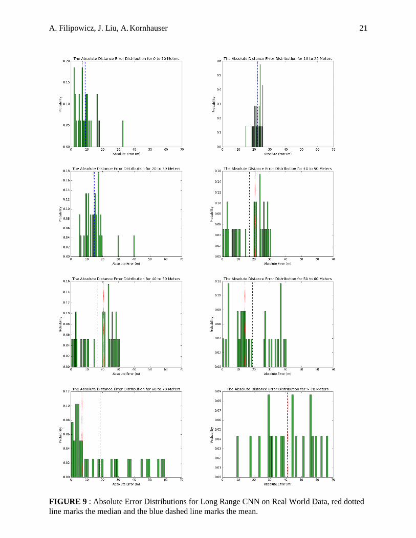
FIGURE 9 : Absolute Error Distributions for Long Range CNN on Real World Data, red dotted

line marks the median and the blue dashed line marks the mean.


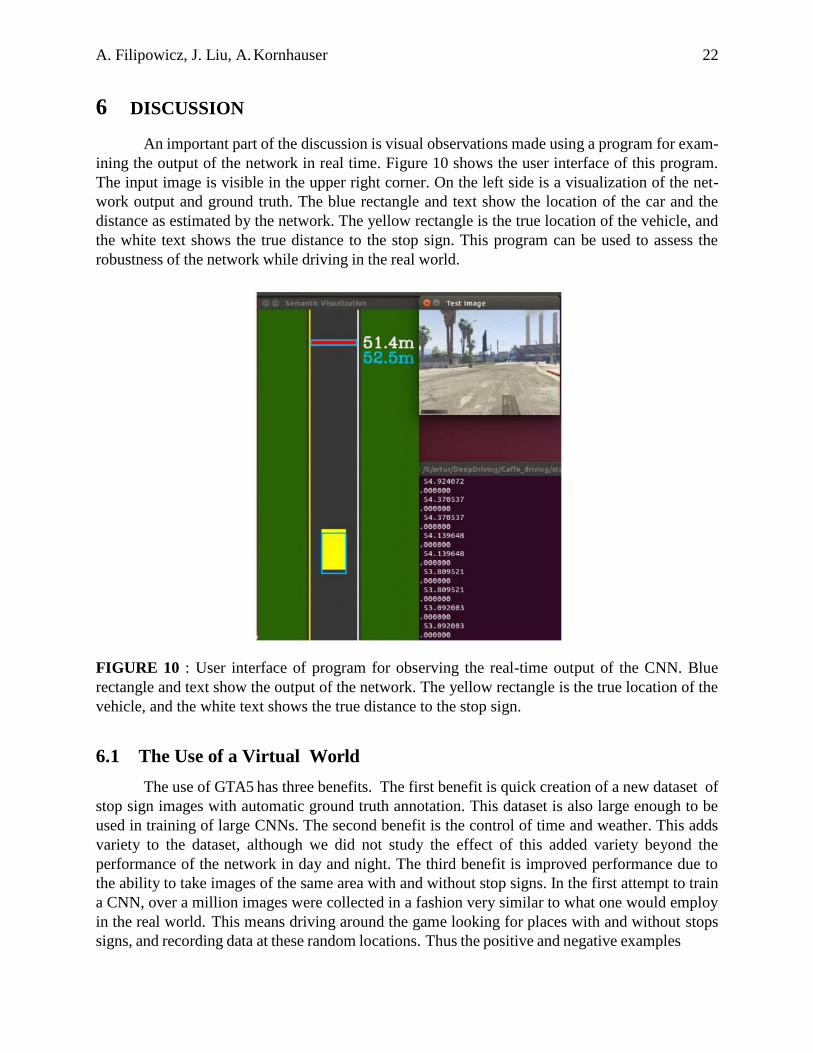
6 DISCUSSION

An important part of the discussion is visual observations made using a program for exam-

ining the output of the network in real time. Figure 10 shows the user interface of this program.

The input image is visible in the upper right corner. On the left side is a visualization of the net-

work output and ground truth. The blue rectangle and text show the location of the car and the

distance as estimated by the network. The yellow rectangle is the true location of the vehicle, and

the white text shows the true distance to the stop sign. This program can be used to assess the

robustness of the network while driving in the real world.

FIGURE 10 : User interface of program for observing the real-time output of the CNN. Blue

rectangle and text show the output of the network. The yellow rectangle is the true location of the

vehicle, and the white text shows the true distance to the stop sign.

6.1 The Use of a Virtual World

The use of GTA5 has three benefits. The first benefit is quick creation of a new dataset of

stop sign images with automatic ground truth annotation. This dataset is also large enough to be

used in training of large CNNs. The second benefit is the control of time and weather. This adds

variety to the dataset, although we did not study the effect of this added variety beyond the

performance of the network in day and night. The third benefit is improved performance due to

the ability to take images of the same area with and without stop signs. In the first attempt to train

a CNN, over a million images were collected in a fashion very similar to what one would employ

in the real world. This means driving around the game looking for places with and without stops

signs, and recording data at these random locations. Thus the positive and negative examples


differed by much more then the presence of a stop sign. The performance of this first long range

CNN was around 55% for all distances on game data and 0% on the real world data. Employing a

strategy of collecting data in the same location with and without a stop sign increased performance

in the range of 0 to 20 meters to around 90% and 80% in the range 20 to 30 meters on in game

data, see Table 5.1. Performance also improved on real world data as well, although a high false

positive rate makes these results less conclusive, see Table 5.2. It is very difficult if not impossible

to obtain these benefits with real world data collection methods.

These unique and useful benefits beg the question of applicability of virtual worlds to real

world situations. Due to time and technological constraints, this study is not able to definitively

answer this question. On the real world data, the Long Range CNN has a false positive rate of

65%, Table 5.3. This is too high to be useful. However, the Short Range CNN has a false positive

rate of only 15%, and a 96% accuracy for 0 to 10 meter, Table 5.3. This is quite promising, but the

errors in distance for this network are very high, Table 5.3, even when the network is accurate. The

reason for the low accuracy may be caused by the lamp post in front of the stop sign, the test

images can be seen in Table 1. Both networks struggled with such occlusions in the game. Low

accuracy would translate to a high error in the distance for examples 20 meters away and further.

In the 0 to 10 meter range where the Short Range CNN is very accurate, there may be a systemic

error caused by differences in the game and real world camera models and data collection setups.

Ultimately, more real world data is necessary to test the CNNs.

6.2 Effects of Distance

According to the test results, the neither CNN cannot reliably detect a stop sign beyond 30

meters. At first, a reason for this may have been the requirement for the network to learn to detect

stop signs 50 and 60 meters away. As seen in Table 1, at those distances and image resolution the

signs are barely visible to the human eye. Requiring the network to correlate these images causes

noisy output at shorter distances as features the network learns from images in the far ranges are

really irrelevant to the task. The results from the Short Range CNN, which was trained on images

where the stop sign is within 40 meters, show that this is true. The false positive rate decreases by

26% and accuracy for 0 to 20 meters increases between 2% and 5%. The average error in distance

deceases by 4 meters when the network correctly identifies a stop sign, Tables 5.1 and

5.2. Interestingly, the accuracy deceased in the ranges of 20 to 30 and 30 to 40 meters while the

error in distance deceased on average 6 to 8 meters when it does identify the stop sign correctly.

This counterintuitive result requires further exploration but a possible cause is the fact that the

Short Range CNN is trained starting with the parameters of the Long Range CNN as oppose to

random parameters. With this approach and image resolution, the signal representing the stop sign

is too small in images beyond 30 meters to be detected reliably.

6.3 Effects of Time and Weather

The CNNs work decisively better during the day. Tables 5.2 and 5.2 detail the differences

in performance of the Short Range CNN during the day and night. The Long Range network has

similar differences. There are two reasons which may be responsible for this difference. Red

taillights might be increasing the false positive rate during the night. The test vehicle’s headlines

do not illuminate the stop sign at distances further than 20 meters. Even at closer distances, the


stop sign may not be illuminated making it difficult to see. It is possible to change the headlights

in the game and a more realistic model of them should be added. On a related note, the networks

appeared to have problems in accurately detecting stops sings at sunsets and sunrises when the

environment have a red hue.

This study does not explore the effects of weather in great detail. Considering that the

number of examples across all the weather conditions have been kept proportional across all the

training and test sets, it does not appear that any one conditions is particularly adverse, at least

when the stop sign is near.

6.4 Effects of Stop Sign Position and Other Observations

There are several important observations made while watching the network outputs in re-

gard to the position and occlusion of the stop sign. The network can detect a stop sign which is

poetically off the screen. However, it is not successful at detecting a stop sign which is partially

occluded by a vehicle. In the design of our dataset, we did not specifically plan occlusions. They

occurred naturally as a consequence of the dynamics of the game engine. Perhaps this is a case

which needs to be more represented in the dataset. Additionally, the network struggles to detect

stop signs on the left side of the road, since they appear mostly on the right side. A source of some

false positives are trees and poles in built environments and a source of some false negatives are

pedestrians. All of these observations suggest that the dataset could be intelligently expended to

increase accuracy.

7 CONCLUSION

We examined a machine learning system approach to stop sign detection and distance es-

timating on individual images. We developed a method to automatically collect labeled data from

Grand Theft Auto 5 and assembled a dataset of 1.4 million images with and without stop signs

across different environments, weather conditions, and times of day. The network can detect 95.5%

of the stops signs within 20 meters with a false positive rate of 5.6% and an average error in dis-

tance of 1.2m to 2.4m on game data. Performance of the CNN degrades beyond 20m and is poor

on real world data requiring further investigation.

This study provides several avenues for future work. One of the most important avenues is

transferring the performance to the real world. This requires the collection of a large dataset of real

world images with measurements. The performance of the model might be improved by expending

the dataset to include more occlusions and stop sign positions. It would also be interesting to

explore the precise effects including weather and time variations has on the performance of the

model. Further research should explore the use a larger images to see if the performance improves

at greater distances and the use of temporal information. Once the limits of this approach for stop

signs are reached and are useful, the scope of the task should be generalized. Instead of just stop

sign detection and localization, the task should be stop object detection and localization, where a

stop object could be stop signs, red and yellow traffic lights, railroad crossings and maybe even

pedestrians, police officers and crosswalks.


8 ACKNOWLEDGMENTS

We gratefully acknowledge the support of NVIDIA Corporation with the donation of the

Tesla K40 GPU used for this research.

References

[1] Gta 5 wiki guide - ign, 2016.

[2] Paths (gta v), 2016.

[3] Vehicles - gta 5 wiki guide - ign, 2016.

[4] Anand R Atreya, Bryan C Cattle, Brendan M Collins, Benjamin Essenburg, Gordon H

Franken, Andrew M Saxe, Scott N Schiffres, and Alain L Kornhauser. Prospect eleven:

Princeton university’s entry in the 2005 darpa grand challenge. Journal of Field Robotics,

23(9):745–753, 2006.

[5] Alexander Barth, Jan Siegemund, and Julian Schwehr. Fast and precise localization at stop

intersections. In Intelligent Vehicles Symposium Workshops (IV Workshops), 2013 IEEE,

pages 75–80. IEEE, 2013.

[6] Christophe Guionneau Christos Dimitrakakis Rémi Coulom Andrew Sumner Bern- hard

Wymann, Eric Espié. TORCS, The Open Racing Car Simulator. http://www.torcs.org, 2014.

[7] Massimo Bertozzi and Alberto Broggi. Gold: A parallel real-time stereo vision system for

generic obstacle and lane detection. IEEE transactions on image processing, 7(1):62–81,

1998.

[8] Chenyi Chen, Ari Seff, Alain Kornhauser, and Jianxiong Xiao. Deepdriving: Learning affor-

dance for direct perception in autonomous driving. In Proceedings of the IEEE International

Conference on Computer Vision, pages 2722–2730, 2015.

[9] Arturo De La Escalera, Luis E Moreno, Miguel Angel Salichs, and José María Armingol.

Road traffic sign detection and classification. IEEE transactions on industrial electronics,

44(6):848–859, 1997.

[10] FHWA. Manual on uniform traffic control devices, 2016.

[11] Andreas Geiger, Philip Lenz, Christoph Stiller, and Raquel Urtasun. Vision meets robotics:

The kitti dataset. International Journal of Robotics Research (IJRR), 2013.

[12] Andreas Geiger, Philip Lenz, and Raquel Urtasun. Are we ready for autonomous driving? the

kitti vision benchmark suite. In Computer Vision and Pattern Recognition (CVPR), 2012

IEEE Conference on, pages 3354–3361. IEEE, 2012.

[13] James J Gibson. The ecological approach to visual perception. Psychology Press, 1979.

http://www.torcs.org/


[14] Erico Guizzo. How google’s self-driving car works. IEEE Spectrum Online, October, 18,

2011.

[15] Lykele Hazelhoff, Ivo Creusen, and Peter HN de With. Robust detection, classification and

positioning of traffic signs from street-level panoramic images for inventory purposes. In

Applications of Computer Vision (WACV), 2012 IEEE Workshop on, pages 313–320. IEEE,

2012.

[16] Christopher J Hill and J Kyle Garrett. AASHTO Connected Vehicle Infrastructure Deployment

Analysis. FHWA-JPO-11-090. FHWA, U.S. Department of Transportation, 2011.

[17] Yangqing Jia, Evan Shelhamer, Jeff Donahue, Sergey Karayev, Jonathan Long, Ross Gir-

shick, Sergio Guadarrama, and Trevor Darrell. Caffe: Convolutional architecture for fast

feature embedding. arXiv preprint arXiv:1408.5093, 2014.

[18] Alex Krizhevsky, Ilya Sutskever, and Geoffrey E Hinton. Imagenet classification with deep

convolutional neural networks. In Advances in neural information processing systems, pages

1097–1105, 2012.

[19] Emil Krsák and Stefan Toth. Traffic sign recognition and localization for databases of traffic

signs. Acta Electrotechnica et Informatica, 11(4):31, 2011.

[20] Yann LeCun, Yoshua Bengio, and Geoffrey Hinton. Deep learning. Nature, 521(7553):436–

444, 2015.

[21] Henry Liu and Bin Ran. Vision-based stop sign detection and recognition system for intel-

ligent vehicles. Transportation Research Record: Journal of the Transportation Research

Board, (1748):161–166, 2001.

[22] Gareth Loy and Nick Barnes. Fast shape-based road sign detection for a driver assistance

system. In Intelligent Robots and Systems, 2004.(IROS 2004). Proceedings. 2004 IEEE/RSJ

International Conference on, volume 1, pages 70–75. IEEE, 2004.

[23] Saturnino Maldonado-Bascon, Sergio Lafuente-Arroyo, Pedro Gil-Jimenez, Hilario Gomez-

Moreno, and Francisco López-Ferreras. Road-sign detection and recognition based on sup-

port vector machines. IEEE transactions on intelligent transportation systems, 8(2):264–278,

2007.

[24] Dean A Pomerleau. Alvinn: An autonomous land vehicle in a neural network. Technical

report, DTIC Document, 1989.

[25] Shuran Song and Jianxiong Xiao. Sliding shapes for 3d object detection in depth images. In

European Conference on Computer Vision, pages 634–651. Springer, 2014.

[26] Paul Theodosis, Lauren Wilson, and SiQi Cheng. Ee368 final project: Road sign detection

and distance estimation in autonomous car application. 2013.

[27] Sebastian Thrun, Mike Montemerlo, Hendrik Dahlkamp, David Stavens, Andrei Aron, James

Diebel, Philip Fong, John Gale, Morgan Halpenny, Gabriel Hoffmann, et al. Stanley: The

robot that won the darpa grand challenge. Journal of field Robotics, 23(9):661–692, 2006.


[28] Radu Timofte, Karel Zimmermann, and Luc Van Gool. Multi-view traffic sign detection,

recognition, and 3d localisation. Machine Vision and Applications, 25(3):633–647, 2014.

[29] Shimon Ullman. Against direct perception. Behavioral and Brain Sciences, 3(03):373–381,

1980.

[30] André Welzel, Andreas Auerswald, and Gerd Wanielik. Accurate camera-based traffic sign

localization. In 17th International IEEE Conference on Intelligent Transportation Systems

(ITSC), pages 445–450. IEEE, 2014.

using virtual worlds, specifically gta5, to learn...

Documents