Karlin and Taylor Ch. 4Reading: Lawler Ch. 3

Resuming from last lecture, why is the nontrivial value of which satisfies the equation

the solution to the extinction probability:

when the mean offspring

One needs to consider what is happening at large epoch by looking at the dynamics.

because probability is continuous

under limits of countable sequences.

But for

so

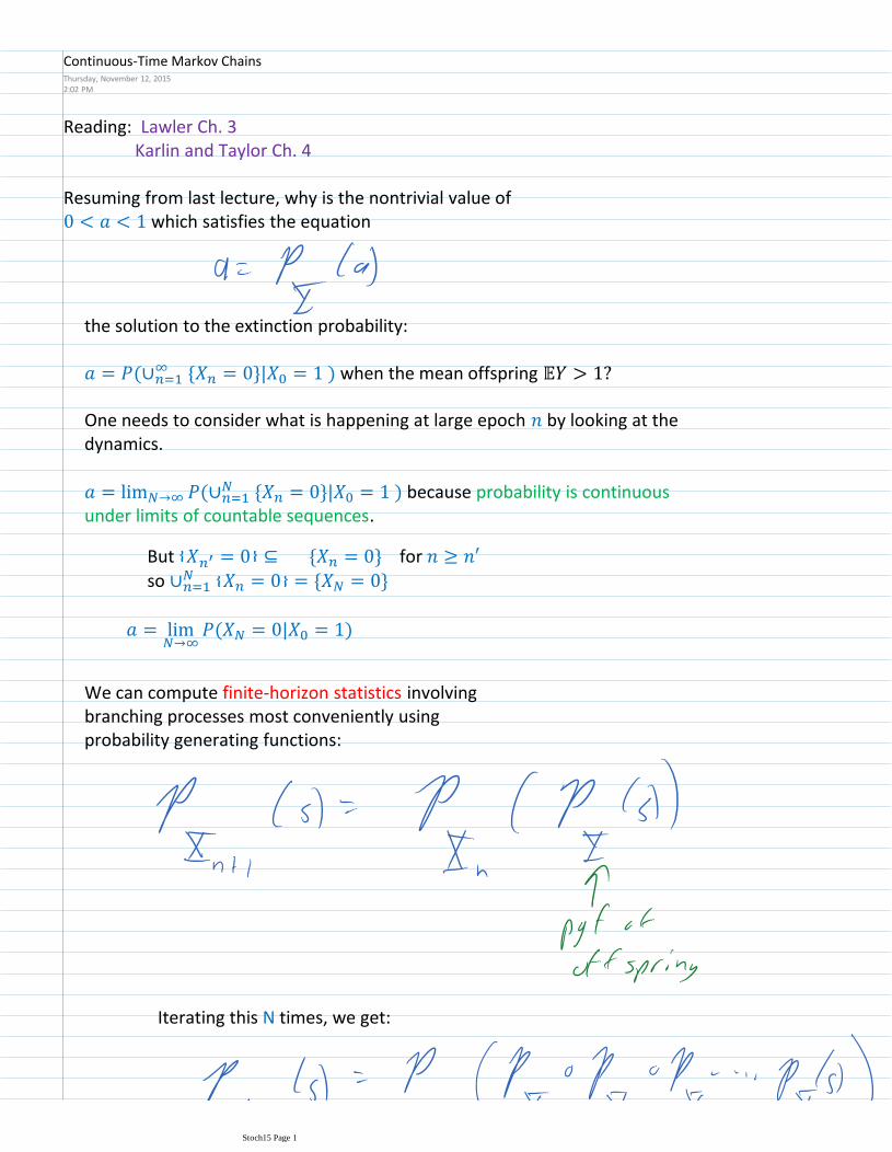
We can compute finite-horizon statistics involving branching processes most conveniently using probability generating functions:

Iterating this N times, we get:

Continuous-Time Markov ChainsThursday, November 12, 20152:02 PM

Stoch15 Page 1

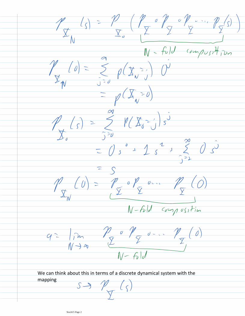
We can think about this in terms of a discrete dynamical system with the mapping

Stoch15 Page 2

One can show, by making appropriate estimates on the behavior of

that the nontrivial fixed point will globally attract all values of . In particularly it attracts the value starting from , so that establishes that the nontrivial solution of

is the correct answer for the probability of extinction starting from one agent.

Continuous-Time Markov Chains

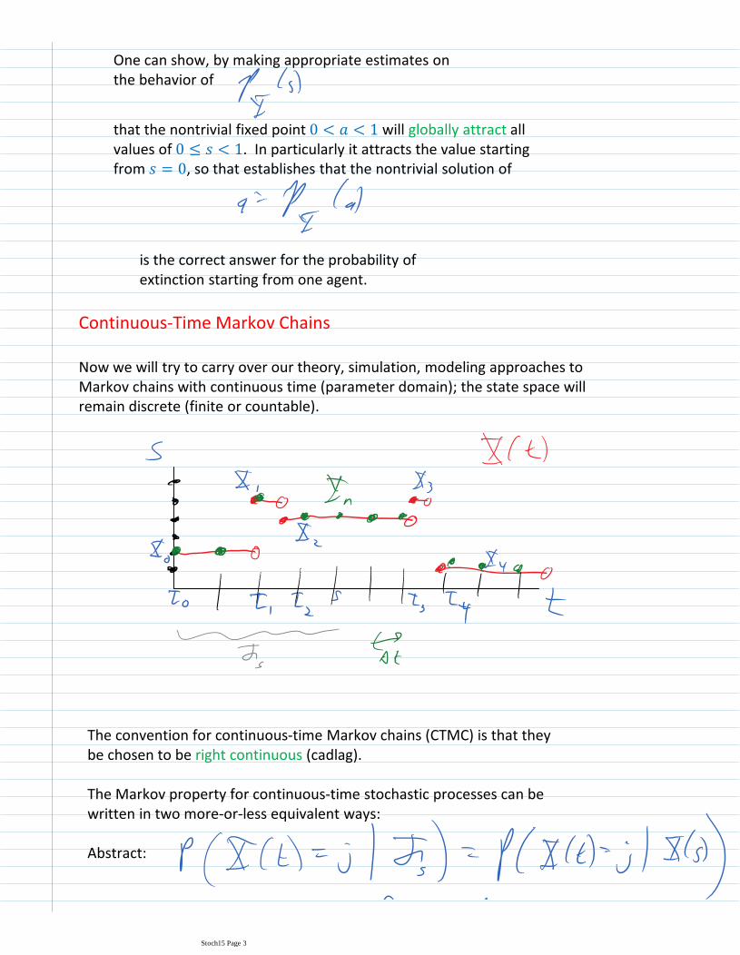
Now we will try to carry over our theory, simulation, modeling approaches to Markov chains with continuous time (parameter domain); the state space will remain discrete (finite or countable).

The convention for continuous-time Markov chains (CTMC) is that they be chosen to be right continuous (cadlag).

The Markov property for continuous-time stochastic processes can be written in two more-or-less equivalent ways:

Abstract:

Stoch15 Page 3

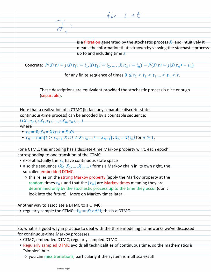
is a filtration generated by the stochastic process , and intuitively it means the information that is known by viewing the stochastic process up to and including time .

Concrete:

for any finite sequence of times

These descriptions are equivalent provided the stochastic process is nice enough (separable).

Note that a realization of a CTMC (in fact any separable discrete-state continuous-time process) can be encoded by a countable sequence:

• for •

where

except actually the have continuous state space•

this relies on the strong Markov property (apply the Markov property at the random times ) and that the are Markov times meaning they are determined only by the stochastic process up to the time they occur (don't look into the future). More on Markov times later…

○

also the sequence forms a Markov chain in its own right, the so-called embedded DTMC

•

For a CTMC, this encoding has a discrete-time Markov property w.r.t. each epoch corresponding to one transition of the CTMC

regularly sample the CTMC: ; this is a DTMC.•Another way to associate a DTMC to a CTMC:

CTMC, embedded DTMC, regularly sampled DTMC•

you can miss transitions, particularly if the system is multiscale/stiff○

the model involves a nonphysical parameter ; the same issue in

Regularly sampled DTMC avoids all technicalities of continuous time, so the mathematics is "simpler" but:

•

So, what is a good way in practice to deal with the three modeling frameworks we've discussed for continuous-time Markov processes

Stoch15 Page 4

the model involves a nonphysical parameter ; the same issue in "simplifying" differential equations to difference equations

○

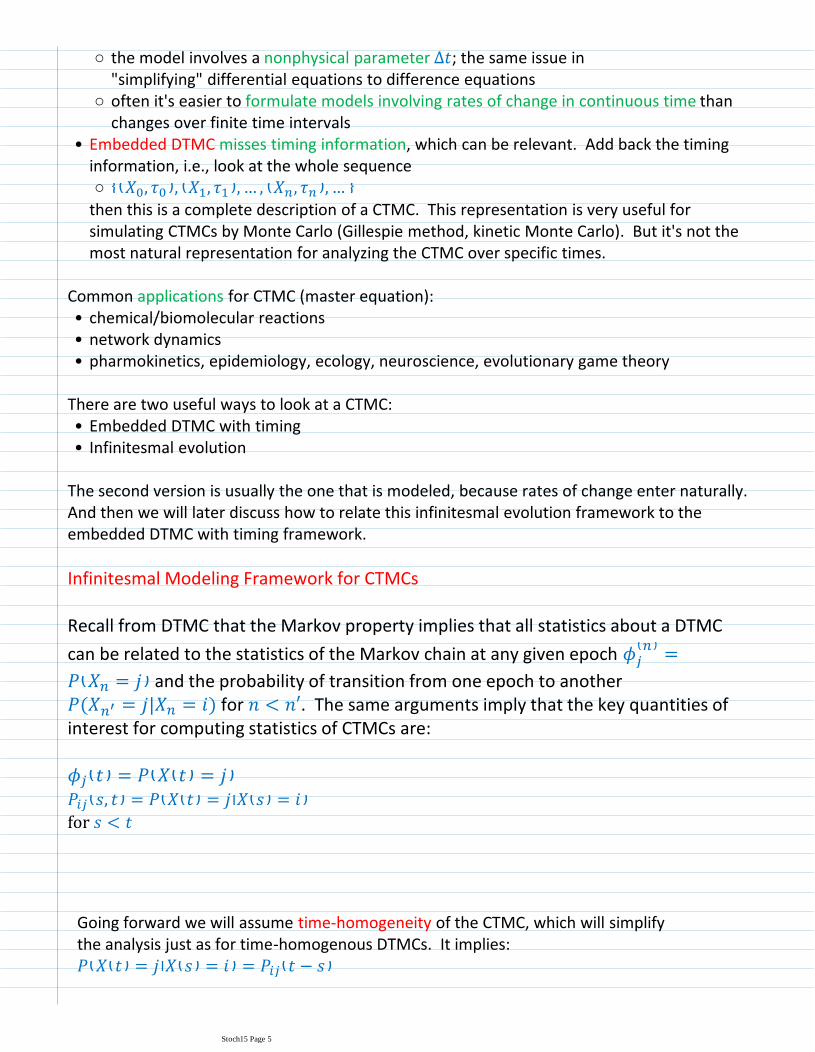
often it's easier to formulate models involving rates of change in continuous time than changes over finite time intervals

○

○

Embedded DTMC misses timing information, which can be relevant. Add back the timing information, i.e., look at the whole sequence

•

then this is a complete description of a CTMC. This representation is very useful for simulating CTMCs by Monte Carlo (Gillespie method, kinetic Monte Carlo). But it's not the most natural representation for analyzing the CTMC over specific times.

chemical/biomolecular reactions•network dynamics•pharmokinetics, epidemiology, ecology, neuroscience, evolutionary game theory•

Common applications for CTMC (master equation):

Embedded DTMC with timing •Infinitesmal evolution•

There are two useful ways to look at a CTMC:

The second version is usually the one that is modeled, because rates of change enter naturally. And then we will later discuss how to relate this infinitesmal evolution framework to the embedded DTMC with timing framework.

Infinitesmal Modeling Framework for CTMCs

Recall from DTMC that the Markov property implies that all statistics about a DTMC

can be related to the statistics of the Markov chain at any given epoch

and the probability of transition from one epoch to another for . The same arguments imply that the key quantities of interest for computing statistics of CTMCs are:

for

.

Going forward we will assume time-homogeneity of the CTMC, which will simplify the analysis just as for time-homogenous DTMCs. It implies:

By discreteness of state we can as we did for DTMCs represent the transition

Stoch15 Page 5

By discreteness of state we can as we did for DTMCs represent the transition probabilities in terms of a matrix, which is now a matrix function which we call the probability transition function

Stoch15 Page 6