real algebraic finite elements and de rham …ccom.ucsd.edu/~agillette/research/kausttalk.pdf ·...

university-logo

Real Algebraic Finite Elements and de RhamCohomology

Andrew Gillette

joint work with

Chandrajit Bajaj

Department of MathematicsInstitute of Computational Engineering and Sciences

University of Texas at Austin

Computational Visualization Center , I C E S (Department of Mathematics Institute of Computational Engineering and Sciences University of Texas at Austin )The University of Texas at Austin KAUST ::: June 2010 1 / 33

university-logo

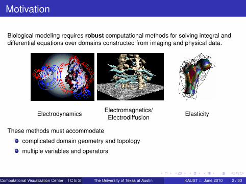
Motivation

Biological modeling requires robust computational methods for solving integral anddifferential equations over domains constructed from imaging and physical data.

Electrodynamics Electromagnetics/Electrodiffusion Elasticity

These methods must accommodate

complicated domain geometry and topology

multiple variables and operators


university-logo

Outline

1 Domain Modeling: Real Algebraic Finite Elements

2 Function Modeling: DEC-deRham Theory

3 Discrete Hodge Stars and Their Inverses


university-logo

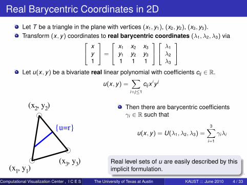
Real Barycentric Coordinates in 2D

Let T be a triangle in the plane with vertices (x1, y1), (x2, y2), (x3, y3).Transform (x , y) coordinates to real barycentric coordinates (λ1, λ2, λ3) via x

y1

=

x1 x2 x3

y1 y2 y3

1 1 1

λ1

λ2

λ3

Let u(x , y) be a bivariate real linear polynomial with coefficients cij ∈ R.

u(x , y) =∑

i+j≤1

cijx iy j

1(x , y )1

2(x , y )2

3(x , y )3

u=r

Then there are barycentric coefficientsγi ∈ R such that

u(x , y) = U(λ1, λ2, λ3) =3∑

i=1

γiλi

Real level sets of u are easily described by thisimplicit formulation.


university-logo

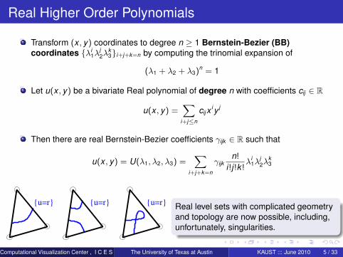
Real Higher Order Polynomials

Transform (x , y) coordinates to degree n ≥ 1 Bernstein-Bezier (BB)coordinates λi

1λj2λ

k3i+j+k=n by computing the trinomial expansion of

(λ1 + λ2 + λ3)n = 1

Let u(x , y) be a bivariate Real polynomial of degree n with coefficients cij ∈ R

u(x , y) =∑

i+j≤n

cijx iy j

Then there are real Bernstein-Bezier coefficients γijk ∈ R such that

u(x , y) = U(λ1, λ2, λ3) =∑

i+j+k=n

γijkn!

i!j!k !λi

1λj2λ

k3

u=r u=r u=r Real level sets with complicated geometryand topology are now possible, including,unfortunately, singularities.


university-logo

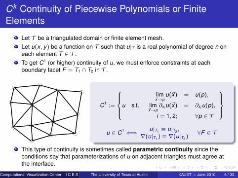
Ck Continuity of Piecewise Polynomials or FiniteElements

Let T be a triangulated domain or finite element mesh.Let u(x , y) be a function on T such that u|T is a real polynomial of degree n oneach element T ∈ T .To get C1 (or higher) continuity of u, we must enforce constraints at eachboundary facet F = T1 ∩ T2 in T .

C1 :=

u s.t.

lim~x→p

u(~x) = u(p),

lim~x→p

∂xi u(~x) = ∂xi u(p),

i = 1, 2; ∀p ∈ T

u ∈ C1 ⇐⇒ u|T1 ≡ u|T2 ,

∇(u|T1 ) ≡ ∇(u|T2 )∀F ∈ T

This type of continuity is sometimes called parametric continuity since theconditions say that parameterizations of u on adjacent triangles must agree atthe interface.


university-logo

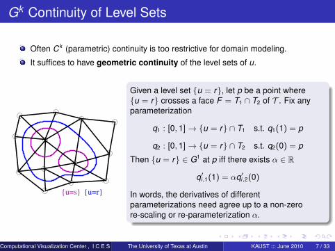
Gk Continuity of Level Sets

Often Ck (parametric) continuity is too restrictive for domain modeling.

It suffices to have geometric continuity of the level sets of u.

u=s u=r

Given a level set u = r, let p be a point whereu = r crosses a face F = T1 ∩ T2 of T . Fix anyparameterization

q1 : [0, 1]→ u = r ∩ T1 s.t. q1(1) = p

q2 : [0, 1]→ u = r ∩ T2 s.t. q2(0) = p

Then u = r ∈ G1 at p iff there exists α ∈ R

q′i,1(1) = αq′i,2(0)

In words, the derivatives of differentparameterizations need agree up to a non-zerore-scaling or re-parameterization α.


university-logo

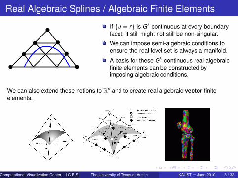
Real Algebraic Splines / Algebraic Finite Elements

If u = r is Gk continuous at every boundaryfacet, it still might not still be non-singular.

We can impose semi-algebraic conditions toensure the real level set is always a manifold.

A basis for these Gk continuous real algebraicfinite elements can be constructed byimposing algebraic conditions.

We can also extend these notions to Rn and to create real algebraic vector finiteelements.


university-logo

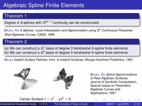
Algebraic Spline Finite Elements

Theorem 1Degree d A-splines with G2d−3 continuity can be constructed.

BAJAJ, XU A-Splines: Local Interpolation and Approximation using Gk Continuous PiecewiseReal Algebraic Curves, CAGD, 1999.

Theorem 2(a) We can construct a G1 basis of degree 3 tetrahedral A-spline finite elements(b) We can construct a G2 basis of degree 5 tetrahedral A-spline finite elements.

BAJAJ Implicit Surface Patches, Intro. to Implicit Surfaces, Morgan Kaufman Publishers, 1997.

Cartan Surface f = x2 − yz2 = 0

BAJAJ, XU Spline Approximationsof Real Algebraic Surfaces,Journal of Symbolic Computation,Special Isssue on ParametricAlgebraic Curves andApplications, 1997


university-logo

Splines and Geometric Modeling

Domain Modeling:Many spline types exist for domain modeling, including A-, B-, NURB- , X, andZ-splines.[SCHONBERG, 1958] and many many others

Real algebraic finite elements provide an efficient method for creating smoothmanifold computational domains with complicated geometry and topology.

The approximation error between a discretization of such domains and theanalytical domain can also be bounded.

Function Modeling:Solutions to PDEs have different, less restrictive continuity requirements than thedomains that support them.

Measuring the error of a function discretized on a discretized domain requiresnew, additional theory.


university-logo

Outline





university-logo

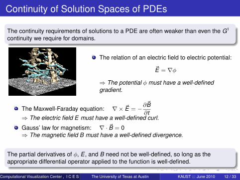
Continuity of Solution Spaces of PDEs

The continuity requirements of solutions to a PDE are often weaker than even the G1

continuity we require for domains.

The relation of an electric field to electric potential:

~E = ∇φ

⇒ The potential φ must have a well-definedgradient.

The Maxwell-Faraday equation: ∇× ~E = −∂~B∂t

⇒ The electric field E must have a well-defined curl.

Gauss’ law for magnetism: ∇ · ~B = 0⇒ The magnetic field B must have a well-defined divergence.

The partial derivatives of φ, E , and B need not be well-defined, so long as theappropriate differential operator applied to the function is well-defined.


university-logo

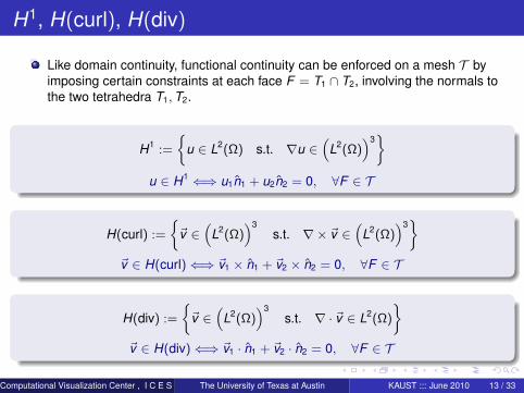
H1, H(curl), H(div)

Like domain continuity, functional continuity can be enforced on a mesh T byimposing certain constraints at each face F = T1 ∩ T2, involving the normals tothe two tetrahedra T1,T2.

H1 :=

u ∈ L2(Ω) s.t. ∇u ∈

(L2(Ω)

)3

u ∈ H1 ⇐⇒ u1n1 + u2n2 = 0, ∀F ∈ T

H(curl) :=

~v ∈

(L2(Ω)

)3s.t. ∇× ~v ∈

(L2(Ω)

)3

~v ∈ H(curl)⇐⇒ ~v1 × n1 + ~v2 × n2 = 0, ∀F ∈ T

H(div) :=

~v ∈

(L2(Ω)

)3s.t. ∇ · ~v ∈ L2(Ω)

~v ∈ H(div)⇐⇒ ~v1 · n1 + ~v2 · n2 = 0, ∀F ∈ T


university-logo

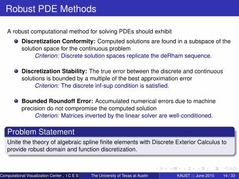
Robust PDE Methods

A robust computational method for solving PDEs should exhibit

Discretization Conformity: Computed solutions are found in a subspace of thesolution space for the continuous problem

Criterion: Discrete solution spaces replicate the deRham sequence.

Discretization Stability: The true error between the discrete and continuoussolutions is bounded by a multiple of the best approximation error

Criterion: The discrete inf-sup condition is satisfied.

Bounded Roundoff Error: Accumulated numerical errors due to machineprecision do not compromise the computed solution

Criterion: Matrices inverted by the linear solver are well-conditioned.

Problem StatementUnite the theory of algebraic spline finite elements with Discrete Exterior Calculus toprovide robust domain and function discretization.


university-logo

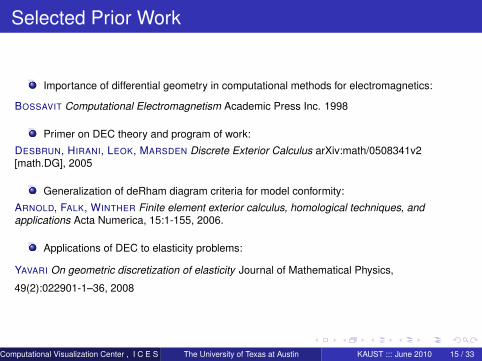
Selected Prior Work

Importance of differential geometry in computational methods for electromagnetics:

BOSSAVIT Computational Electromagnetism Academic Press Inc. 1998

Primer on DEC theory and program of work:

DESBRUN, HIRANI, LEOK, MARSDEN Discrete Exterior Calculus arXiv:math/0508341v2[math.DG], 2005

Generalization of deRham diagram criteria for model conformity:

ARNOLD, FALK, WINTHER Finite element exterior calculus, homological techniques, andapplications Acta Numerica, 15:1-155, 2006.

Applications of DEC to elasticity problems:

YAVARI On geometric discretization of elasticity Journal of Mathematical Physics,

49(2):022901-1–36, 2008


university-logo

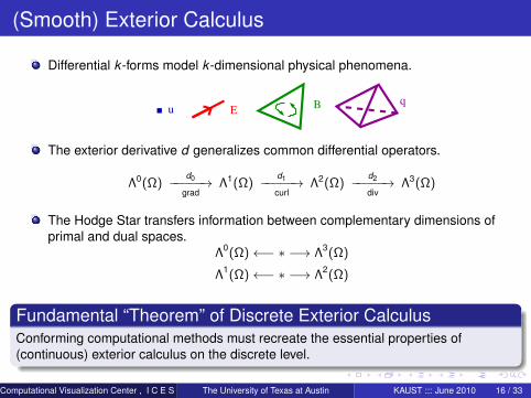
(Smooth) Exterior Calculus

Differential k -forms model k -dimensional physical phenomena.

EB q

u

The exterior derivative d generalizes common differential operators.

Λ0(Ω)d0−−−−−→

gradΛ1(Ω)

d1−−−−−→curl

Λ2(Ω)d2−−−−−→div

Λ3(Ω)

The Hodge Star transfers information between complementary dimensions ofprimal and dual spaces.

Λ0(Ω)←− ∗ −→ Λ3(Ω)

Λ1(Ω)←− ∗ −→ Λ2(Ω)

Fundamental “Theorem” of Discrete Exterior CalculusConforming computational methods must recreate the essential properties of(continuous) exterior calculus on the discrete level.


university-logo

Discrete Exterior Calculus

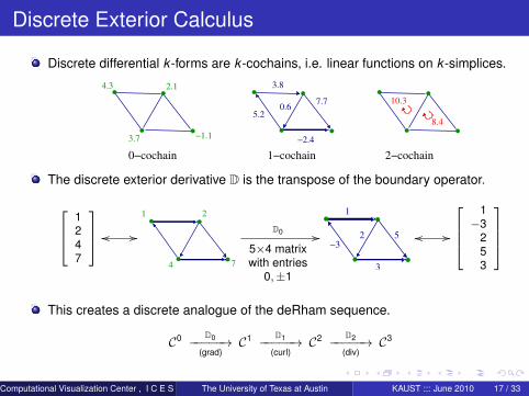
Discrete differential k -forms are k -cochains, i.e. linear functions on k -simplices.

8.4

10.3

3.7

2.14.3

−1.1

0−cochain 1−cochain 2−cochain

3.8

7.7

5.20.6

−2.4

The discrete exterior derivative D is the transpose of the boundary operator.

1247

oo //

1 2

4 7

D0

5×4 matrixwith entries

0,±1

//

1

2

−3

3

5

1−3

253

//oo

This creates a discrete analogue of the deRham sequence.

C0 D0−−−−−→(grad)

C1 D1−−−−−→(curl)

C2 D2−−−−−→(div)

C3


university-logo

The Importance of Cohomology

Λ0d0

grad// Λ1

d1

curl// Λ2

d2

div// Λ3

C0D0 // C1

D1 // C2D2 // C3

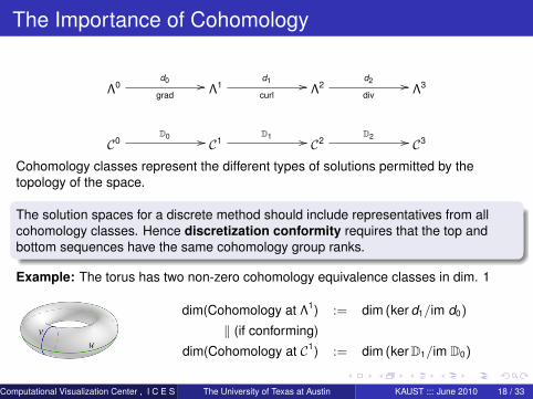
Cohomology classes represent the different types of solutions permitted by thetopology of the space.

The solution spaces for a discrete method should include representatives from allcohomology classes. Hence discretization conformity requires that the top andbottom sequences have the same cohomology group ranks.

Example: The torus has two non-zero cohomology equivalence classes in dim. 1

dim(Cohomology at Λ1) := dim (ker d1/im d0)

‖ (if conforming)

dim(Cohomology at C1) := dim (kerD1/im D0)


university-logo

Finite element methods

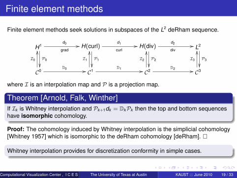
Finite element methods seek solutions in subspaces of the L2 deRham sequence.

H1d0

grad//

P0

H(curl)d1

curl//

P1

H(div)d2

div//

P2

L2

P3

C0

D0 //

I0

OO

C1D1 //

I1

OO

C2D2 //

I2

OO

C3

I3

OO

where I is an interpolation map and P is a projection map.

Theorem [Arnold, Falk, Winther]If Ik is Whitney interpolation and Pk+1dk = DkPk then the top and bottom sequenceshave isomorphic cohomology.

Proof: The cohomology induced by Whitney interpolation is the simplicial cohomology[Whitney 1957] which is isomorphic to the deRham cohomology [deRham].

Whitney interpolation provides for discretization conformity in simple cases.


university-logo

Discrete Exterior Calculus

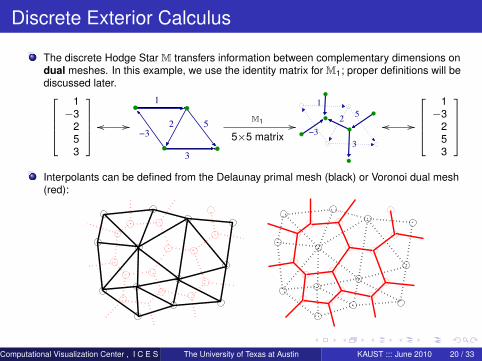
The discrete Hodge Star M transfers information between complementary dimensions ondual meshes. In this example, we use the identity matrix for M1; proper definitions will bediscussed later.

1−3

253

oo //

1

2

−3

3

5M1

5×5 matrix//

3

5

−3

2

1

1−3

253

//oo

Interpolants can be defined from the Delaunay primal mesh (black) or Voronoi dual mesh(red):


university-logo

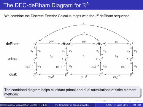
The DEC-deRham Diagram for R3

We combine the Discrete Exterior Calculus maps with the L2 deRham sequence.

deRham: H1grad //

P0

∗

##H(curl) curl //

P1

∗

!!H(div)

div //

P2

L2

P3

primal: C0

D0 //

I0

OO

M0

C1D1 //

I1

OO

M1

C2D2 //

I2

OO

M2

C3

I3

OO

M3

dual: C3

(M0)−1

OO

C2

(D0)Too

(M1)−1

OO

C1

(D1)Too

(M2)−1

OO

C0

(D2)Too

(M3)−1

OO

The combined diagram helps elucidate primal and dual formulations of finite elementmethods.


university-logo

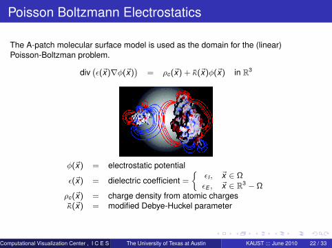
Poisson Boltzmann Electrostatics

The A-patch molecular surface model is used as the domain for the (linear)Poisson-Boltzman problem.

div(ε(~x)∇φ(~x)

)= ρc(~x) + κ(~x)φ(~x) in R3

φ(~x) = electrostatic potential

ε(~x) = dielectric coefficient =

εI , ~x ∈ Ω

εE , ~x ∈ R3 − Ωρc(~x) = charge density from atomic chargesκ(~x) = modified Debye-Huckel parameter


university-logo

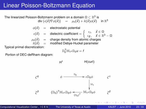
Linear Poisson-Boltzmann Equation

The linearized Poisson-Boltzmann problem on a domain Ω ⊂ R3 isdiv(ε(~x)∇φ(~x)

)= ρc(~x) + κ(~x)φ(~x) in R3

φ(~x) = electrostatic potential

ε(~x) = dielectric coefficient =

εI , ~x ∈ ΩεE , ~x ∈ R3 − Ω

ρc(~x) = charge density from atomic chargesκ(~x) = modified Debye-Huckel parameter

Typical primal discretization:DT

0 M1εD0u = fPortion of DEC-deRham diagram:

H1 H(curl)

C0 φD0 // εD0φ

M1

C1

C3 (D0)TM1εD0φ M1εD0φ(D0)T

oo C2


university-logo

Linear Poisson-Boltzmann Equation

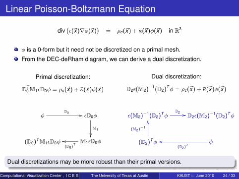
div(ε(~x)∇φ(~x)

)= ρc(~x) + κ(~x)φ(~x) in R3

φ is a 0-form but it need not be discretized on a primal mesh.

From the DEC-deRham diagram, we can derive a dual discretization.

Primal discretization:

DT0 M1εD0φ = ρc(~x) + κ(~x)φ(~x)

φD0 // εD0φ

M1

(D0)TM1εD0φ M1εD0φ

(D0)Too

Dual discretization:

D2ε(M2)−1(D2)Tφ = ρc(~x) + κ(~x)φ(~x)

ε(M2)−1(D2)TφD2 // D2ε(M2)−1(D2)Tφ

(D2)Tφ

(M2)−1

OO

φ(D2)T

oo

Dual discretizations may be more robust than their primal versions.


university-logo

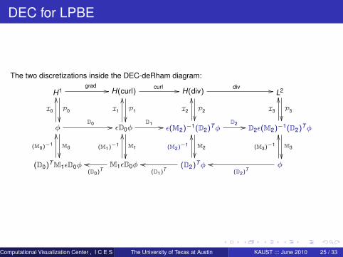
DEC for LPBE

The two discretizations inside the DEC-deRham diagram:

H1grad //

P0

H(curl)curl //

P1

H(div)div //

P2

L2

P3

φ

D0 //

I0

OO

M0

εD0φD1 //

I1

OO

M1

ε(M2)−1(D2)TφD2 //

I2

OO

M2

D2ε(M2)−1(D2)Tφ

I3

OO

M3

(D0)TM1εD0φ

(M0)−1

OO

M1εD0φ(D0)T

oo

(M1)−1

OO

(D2)Tφ

(M2)−1

OO

(D1)Too φ

(D2)Too

(M3)−1

OO


university-logo

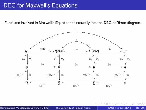
DEC for Maxwell’s Equations

Functions involved in Maxwell’s Equations fit naturally into the DEC-deRham diagram:

H1grad //

P0

∗

##H(curl) curl //

P1

∗

!!H(div)

div //

P2

L2

P3

φ

D0 //

I0

OO

M0

~ED1 //

I1

OO

M1

~BD2 //

I2

OO

M2

q

I3

OO

M3

q

(M0)−1

OO

~B(D0)T

oo

(M1)−1

OO

~E(D1)T

oo

(M2)−1

OO

φ(D2)T

oo

(M3)−1

OO


university-logo

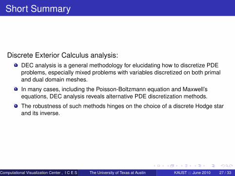
Short Summary

Discrete Exterior Calculus analysis:DEC analysis is a general methodology for elucidating how to discretize PDEproblems, especially mixed problems with variables discretized on both primaland dual domain meshes.

In many cases, including the Poisson-Boltzmann equation and Maxwell’sequations, DEC analysis reveals alternative PDE discretization methods.

The robustness of such methods hinges on the choice of a discrete Hodge starand its inverse.


university-logo

Outline





university-logo

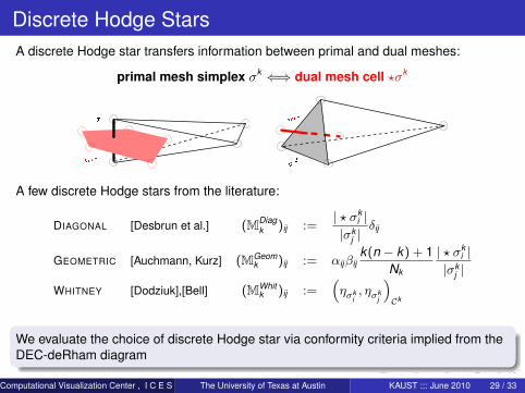
Discrete Hodge StarsA discrete Hodge star transfers information between primal and dual meshes:

primal mesh simplex σk ⇐⇒ dual mesh cell ?σk

A few discrete Hodge stars from the literature:

DIAGONAL [Desbrun et al.] (MDiagk )ij :=

| ? σki |

|σkj |

δij

GEOMETRIC [Auchmann, Kurz] (MGeomk )ij := αijβij

k(n − k) + 1Nk

| ? σki |

|σkj |

WHITNEY [Dodziuk],[Bell] (MWhitk )ij :=

(ησk

i, ησk

j

)Ck

We evaluate the choice of discrete Hodge star via conformity criteria implied from theDEC-deRham diagram


university-logo

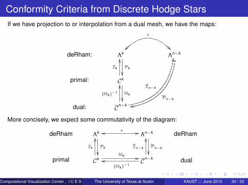
Conformity Criteria from Discrete Hodge StarsIf we have projection to or interpolation from a dual mesh, we have the maps:

deRham: Λk

Pk

∗

Λn−k

Pn−k

qq

primal: Ck

Ik

OO

Mk

dual: Cn−k

(Mk )−1

OO In−k

MM

More concisely, we expect some commutativity of the diagram:

deRham Λk

Pk

oo ∗ // Λn−k

Pn−k

deRham

primal Ck

Ik

OO

Mk //Cn−k

(Mk )−1oo

In−k

OO

dual


university-logo

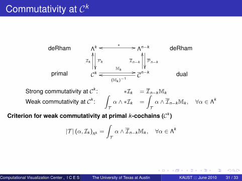
Commutativity at Ck

deRham Λk

Pk

oo ∗ // Λn−k

Pn−k

deRham

primal Ck

Ik

OO

Mk //Cn−k

(Mk )−1oo

In−k

OO

dual

Strong commutativity at Ck : ∗Ik = In−kMk

Weak commutativity at Ck :∫Tα ∧ ∗Ik =

∫Tα ∧ In−kMk , ∀α ∈ Λk

Criterion for weak commutativity at primal k -cochains (Ck )

|T | (α, Ik )Λk =

∫Tα ∧ In−kMk , ∀α ∈ Λk


university-logo

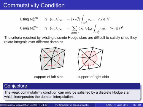
Commutativity Condition

Using MDiag0 : |T | (α, λi )H1 = | ? σ0

i |∫?σ0

i

αµ, ∀α ∈ H1

Using MWhit0 : |T | (α, λi )H1 =

∑vertex j

(λi , λj )H1

∫?σ0

i

αµ, ∀α ∈ H1

The criteria required by existing discrete Hodge stars are difficult to satisfy since theyrelate integrals over different domains.

support of left side support of right side

ConjectureThe weak commutativity condition can only be satisfied by a discrete Hodge starwhich incorporates the domain interpolation.


university-logo

Thank You / Shukran

Thanks for inviting us to visit

Slides available at http://www.ma.utexas.edu/users/agillette


real algebraic finite elements and de rham …ccom.ucsd.edu/~agillette/research/kausttalk.pdf ·...

Documents