real estate booms and endogenous productivity...

Real Estate Booms and Endogenous Productivity Growth∗

Yu Shi†

November 13, 2016JOB MARKET PAPER

Click Here for the Latest Version

Abstract

This paper argues that real estate booms negatively affect productivity growth through an inef-ficient allocation of entrepreneurial talent across sectors. Using matched firm-to-firm shareholdingand balance sheet data, I document that the recent real estate boom in China attracted more talentedmanufacturing entrepreneurs to the real estate sector. These entrepreneurs diverted their resourcesto real estate and away from manufacturing, resulting in lower investments, R&D expenditures, andproductivity growth in their manufacturing businesses. I find empirical evidence that the observedallocation of entrepreneurial talent is driven by more talented manufacturing entrepreneurs beingless financially constrained, and thus able to overcome the entry barrier. I then model the businesschoices of entrepreneurs with heterogeneous talent in an environment where the financial market isimperfect and the real estate sector faces a costly barrier to entry. In my model, more talented man-ufacturers accumulate more wealth through self-financing, and they are therefore less constrainedby the cost of entering the real estate sector in the event of a real estate boom. Inefficient talent al-location arises if more talented manufacturing entrepreneurs do not have a comparative advantagein real estate. A structural estimation of the model confirms the existence of an inefficient allocationof entrepreneurial talent during the Chinese real estate boom.

∗I am extremely grateful to my advisors Daron Acemoglu, Robert Townsend, and Jonathan Parker for their invaluableguidance and support. I thank Ricardo Caballero, Emi Nakamura, Marios Angeletos, Ivan Werning, Jón Steinsson, Alp Sim-sek, Arnaud Costinot, David Berger, Johannes Stroebel, David Atkin, Glenn Ellison, Alberto Abadie, Anna Mikusheva, BillWheaton, and participants in MIT Macro Lunch, MIT Applied Micro Lunch, and MIT Macroeconomics Seminar for helpfulcomments. This paper benefited from numerous discussions with Kai Yan. I also thank Greg Howard, Sebastian Fanelli, Lud-wig Straub, Rachael Meager, Vivek Bhattacharya, John Firth, Otis Reid, Daniel Green, Jie Bai, Yan Ji, Chen Lian, Alex He,Rodrigo Adao, Yao Zeng, Yixin Chen, and Chen Sun for sharing their comments on this paper. I am indebted to Xiaobo Zhangand Wu Zhu for help in processing the confidential data from the China State Administration for Industry and Commerce. Ithank the MIT STL Lab and MIT Economics Department Shultz Fund for financial support. Finally, I thank Xiaowen Yang forhelp in working with the GIS data. Sizhu Lu provided excellent research assistance for this paper. All errors are my own.

†Economics Department, Massachusetts Institute of Technology ([email protected])

1

http://economics.mit.edu/files/12312

1 Introduction

This paper studies the interaction of real estate prices and aggregate productivity. Figure 11 doc-uments the relationship between real estate prices and total factor productivity (TFP) in real estateboom episodes in select countries. As the figure shows, in the real estate booms in Ireland, Aus-tralia, and China, productivity declined significantly while house prices were still rising, well beforethe peak of the boom-bust cycle. I consider the hypothesis that the real estate boom caused the lossin productivity growth, rather than both being caused by a third factor or causation running in thereverse direction. The recent literature emphasizes that rising real estate prices can cause increasesin demand through the relaxation of collateral-based credit constraints (Chaney, Thesmar, and Sraer,2012; Mian and Sufi, 2011; Kerr, Kerr, and Nanda, 2015), or that real estate becomes an asset with arational pricing bubble (Martin and Ventura, 2012). In either situation, an increase in house pricesincreases the efficiency of the talent allocation by allowing unproductive agents to transfer wealth tothe productive ones. Neither approach, therefore, is consistent with a slowdown of TFP during a realestate boom.

Figure 1: Real Estate Prices and Total Factor Productivity

I propose a novel channel through which a real estate boom can cause productivity losses in an

1Data sources: OECD, Penn World Table, St.Louis Fed, the Economist global house price database

2

economy with an imperfect financial market. During a real estate boom, high returns on the realestate market attract entrepreneurs from other sectors to reallocate resources to the real estate sector.Starting up real estate businesses, however, requires a significant investment up front for land pur-chases, thus creating an entry barrier. In the presence of an imperfect financial market, only successfulentrepreneurs who have accumulated enough wealth can overcome such an entry barrier. But theseentrepreneurs have been proven to have a high degree of talent in the non-real estate sector. It is thennatural to believe that entrepreneurs with a comparative advantage outside the construction sectorare those who enter it, leaving low-productivity entrepreneurs in the non-real estate sector and thuslowering aggregate productivity. In sum, the imperfect financial market can create a distortion in theallocation of entrepreneurial talents.

In this paper, I use the unique institutional features in China and rich, disaggregated data to iden-tify this new channel. Since the late 1990s, the Chinese government has lifted a series of regulationsto liberalize the housing market and to privatize the construction of residential housing. In 2002, ur-ban land sales started to open to private real estate developers. During the same period, the urbanpopulation increased by 90% from 1995 to 2010, in contrast to a mere 10% increase in total population.The stimulus for both housing demand and housing supply led to a prolonged housing boom. Theoverall growth in house prices in the past decade was over 10% per annum on a compounded basis(Deng, Gyourko and Wu, 2015). Meanwhile, the overall growth in the quantity of residential housingwas over 20% per annum2.

I first show that the raw patterns in the data are consistent with a significant number of better-performing and also larger manufacturing firms diverting their limited resources to the real estatesector. In my sample, around 20% of the newly established real estate development businesses wereheld by existing companies in industries other than real estate or finance3. Manufacturing companiesthat entered the real estate development industry controlled 30% of the total fixed assets in the manu-facturing sector and also exhibited higher investment rates, R&D intensities, and productivity levelsprior to entry. In addition, entering the real estate development sector resulted in a decline in invest-ment, R&D expenditures, and productivity in these manufacturing companies’ original businesses.This suggests that entrepreneurs redirected their limited resources of physical and human capital tothe real estate sector.

However, the pattern of manufacturing entrepreneurs reallocating their resources is prone to acritical endogeneity challenge: the likelihood of entering the real estate sector is correlated with in-vestment opportunities an entrepreneur has in the manufacturing sector. I provide causal evidencethat the declines in investment, R&D, and productivity are indeed driven by entry into the real estate

2The quantity growth is calculated by the author from an official National Bureau of Statistics publication.3A large number of new entrants in the real estate sector also exists in other real estate booms. For example, Schmalz,

Sraer and Thesmar (2015) document that when France experienced the first wave of their housing boom, over 18% of thenewly created businesses in 1998 were construction companies. Similarly, Corradin and Popov (2015) find that during thegreat housing boom in the US, 15.5% of new business owners choose to operate in the construction industry. In contrast, theconstruction industry only accounts for 0.8% of establishments in the US.

3

sector using two different identification strategies. The first strategy is an instrumental variable (IV)approach. I instrument entrepreneurs’ decisions on entering the real estate sector with the interactionof city-specific land supply inelasticity, firm-specific potential connections with the local land bureauminister, and national real estate prices. The identifying assumption is that when real estate prices areappreciating, the connected firms in a city with a flexible land supply do not necessarily gain more orless advantage in manufacturing compared to a similar firm in a city with an inflexible land supply.The land supply inelasticity, following Saiz (2010) and Mian and Sufi (2011), works as a proxy forreturns in the housing market. This variable is arguably uncorrelated with local income and output.It also has a negative correlation with quantity growth on the housing market, suggesting that landsupply elasticity in China is unlikely to correlate with local housing demand. The potential connec-tions between entrepreneurs and local land bureau ministers serve as a proxy for individual abilityto enter the land market. I construct this variable as an indicator of whether or not a firm executiveshares the same birth county with his local regulators, which eliminates the endogeneity concern inthe formation of a social network. I further control for the two-way interaction terms to capture anypossible differences between politically connected firms and other firms that were not connected. Formy second empirical strategy, I estimate the causal effect using a propensity score matching approach.In particular, I match manufacturing firms based on their size, profitability, and pre-entry investmentactivities to evaluate the effect of entering the real estate sector on manufacturing production. Theestimates from both approaches are comparable in magnitude.

Second, I discuss a theoretical framework that demonstrates how the social efficiency of the ob-served allocation of entrepreneurial talent depends on the comparative advantage of entrepreneurs.In a real estate boom, it is constrained inefficient to reallocate more talented manufacturing en-trepreneurs to the real estate sector if they also have a comparative advantage in the manufactur-ing sector. The financial market imperfection is key to understanding this result. Prior to the realestate boom, the self-financing mechanism results in a positive correlation between wealth and en-trepreneurial talent in the manufacturing sector. With a rapidly appreciating real estate prices, en-trepreneurs face a higher return on capital in the real estate sector. Nevertheless, only entrepreneurswith enough wealth can overcome the entry barrier in the real estate sector. When rich and talentedentrepreneurs without a comparative advantage in real estate enter the real estate market, land pricesrise. The resulting high land prices constrain untalented and poor manufacturing entrepreneurs, whohave a comparative advantage in the real estate sector. A social planner who is aware of the pecu-niary externality imposes lower land prices so entrepreneurs with a comparative advantage in thereal estate sector are less constrained.

I also discuss several policy tools using the theoretical framework, including a liberalization of thefinancial market, a reduction of the entry barrier in the real estate sector, and a taxation on the returnsfrom operating in the real estate sector. Liberalizing the financial market improves social welfare butalso aggravates the social inefficiency. In a more liberalized financial market, the already wealthy

4

entrepreneurs can borrow more, which further increases land prices. As a result, more entrepreneurswith low wealth and the comparative advantages in the real estate sector are constrained by the entrybarrier. A lower entry barrier in the real estate sector has an ambiguous impact on welfare, as moreuntalented entrepreneurs continue operating their businesses. A taxation on real estate returns canimprove both social welfare and efficiency. I also provide quantitative evaluation on the three policytools.

Finally, I provide empirical evidence that talented manufacturing entrepreneurs have both an ab-solute advantage and comparative advantage in the manufacturing sector. Using data that matchesthe real estate business and the manufacturing business of the same entrepreneur, I structurally esti-mate the correlation between the entrepreneurs’ comparative advantage in the real estate sector andtheir absolute advantage (talent) in the manufacturing sector. In my model, it is equivalent to esti-mating the return on capital in the real estate business as a function of the TFP in the manufacturingbusiness. I first employ a Solow-residual type of estimate (Basu and Fernald, 1997) for estimatingthe entrepreneurial talent in the manufacturing sector using firm-level data prior to the land mar-ket reform in 2002. I then regress the entrepreneurs’ returns on capital in the real estate sector onthe estimated manufacturing talents. There are two issues with this structural estimation. First, themanufacturing talent of entrepreneurs are estimated with errors, so there is attenuation bias. Second,selection bias exists because I do not observe the return on capital in real estate for manufacturing en-trepreneurs who did not enter the real estate sector. To correct for the first bias, I impose an empiricalBayes adjustment on the estimates of entrepreneurs’ manufacturing talent, as is commonly used inthe literature on estimating the value added of teachers (Kane and Staiger, 2008; Meghir and Rivkin,2011; Chetty, Friedman, and Rockoff, 2014). For the second bias, I apply a nonparametric approach(Das, Newey, and Vella, 2003) that proxies for the selection bias using a non-parametric function ofthe entrepreneur-specific propensity score for entering the real estate sector. The results indicate thatthe return from housing production is less sensitive to entrepreneurial skills than that from manufac-turing production. Thus, I conclude that a run-up in house prices would lead to an inefficient loss inaggregate productivity.

The new channel I propose and identify in this paper has two appealing theoretical features.First, it does not require a housing bubble to generate an inefficient allocation of entrepreneurialtalents. The recent discussions on misallocations during housing booms focus on the bubble episodes(Charles, Hurst and Notowidigdo, 2015; Chen and When, 2014), and hence inefficiencies exist by defi-nition. In my model, as long as housing construction has a high entry barrier and the financial marketis imperfect, misallocation likely exists. This takes place even if the housing boom is driven by fun-damental factors such as rapid urbanization. Second, the model can be used to study other boomingsectors, as long as they also require a high capital expenditure up front. Another prominent exampleis that countries typically are lacking of the ability to grow following a natural resource boom, as withthe so-called “the Dutch disease” (Rajan and Subramanian, 1994; Torvik, 2001; Allcott and Keniston,

5

2014).This paper is related to several strands of literature. It relates broadly to the literature on the re-

lationship between house prices and the macroeconomy. Previous research outlines several channelsthrough which housing can influence the economy. For example, Mian and Sufi (2011), Mian, Sufiand Rao (2013) and Chaney, Thesmar, and Sraer (2012) propose the household balance sheet channeland firm collateral channel. In linking real estate booms with productivity growth, Anzoategui et al.(2016) argues for an exogenous cycle of R&D activities. This paper proposes another channel throughwhich real estate prices can endogenously affect aggregate productivity growth, namely through thedecisions of entrepreneurs. I argue that when combined with an imperfect financial market, a sig-nificant and rapid price appreciation in the real estate market can result in inefficient entrepreneurialtalent allocation across industries.

In addition, this paper complements the literature that studies the long-run impact of a housingboom from the perspective of entrepreneurs. One strand of the work in this area focuses on howhouse price appreciation promotes new businesses (Hurst and Lusardi, 2004; Schmalz, Sraer andThesmar, 2015; Kerr, Kerr, and Nanda, 2015). They essentially explore the collateral value of real es-tate properties. The paper most similar in spirit to mine is Charles, Hurst, and Notowidigdo (2015).They argue that booming labor demand in the construction sector results in a decline in college atten-dance. This paper, by contrast, emphasizes the distortion on entrepreneurs’ occupation choice and itsconsequences to aggregate productivity.

This paper also relates closely to the discussion on the allocation of talent. Murphy, Shleifer,and Vishny (1991) propose that certain social reward structures may result in more talented peo-ple specializing in unproductive activities such as rent seeking, leading to stagnation. More relatedto my paper, Legros and Newman (2002) argue that certain financial imperfections can lead to thenon-monotonic specialization of entrepreneurs, which corresponds to my empirical observations. Itake their arguments one step further to show that in real estate booms, the misallocation of en-trepreneurial talent inefficiently reduces productivity growth through rising land prices without as-suming real estate production as a rent-seeking behavior. I also show that simple policy tools can beused to correct for such an inefficiency in entrepreneurial talent allocation.

Moreover, this paper makes a significant contribution to the literature on misallocation and eco-nomic growth. The majority of work has studied resource misallocation, which occurs when the mostproductive entrepreneurs do not acquire enough capital input for production, but does not touch di-rectly on the misallocation of entrepreneurial talent (Hsieh and Klenow, 2009; Song et al. 2011; Bueraand Shin, 2013). Other papers document that capital entry barriers prevent productive entrepreneursfrom producing (Buera, Kaboski, and Shin, 2012; Midrigan and Xu, 2014). However, they do not ex-plore the comparative advantage of the entrepreneurs, and thus miss an important channel via theirendogenous selection into different industries. This paper complements the literature by not onlyproviding a theoretical framework, but also by offering substantial empirical evidence on talent mis-

6

allocation and its impact on economic growth. The quantitative exercise of this paper builds on Songet al. (2011) to model the Chinese economy in transition to a balanced growth path. I extend theirquantitative framework by adding a housing boom and heterogeneous entrepreneurs.

Last but not least, this paper fits into the growing literature studying the Chinese real estate mar-ket. Fang et al. (2014) and Deng, Gyourko, and Wu (2015) document a rapid real estate price appre-ciation and large variation in city-level real estate prices in China. Chen et al. (2015), Chen and Wen(2014), and Shi et al. (2016) discuss the misallocation of capital and labor in this real estate, under thehypothesis that the real estate boom is a bubble episode. Given that real estate prices in China are stillgoing strong in the first-tier and second-tier cities, this paper suggests a framework that inefficiencyexists without assuming a bubble episode. I also propose policy tools to reduce the inefficiency inentrepreneurial talent allocation.

The rest of the paper is organized as follows. Section 2 describes the institutional backgroundof the real estate market reform and the housing boom in China. I also provide a comprehensivedescription of the Chinese data sets. Section 3 documents the empirical findings on the allocationof entrepreneurial talent in the recent Chinese real estate boom. In particular, I estimate the causaleffect of entering the real estate sector on manufacturing firms’ original businesses. Section 4 de-scribes a two-period general equilibrium model for evaluating the social efficiency of the observedentrepreneurial talent allocation. I discuss several policy tools that can help with improving the socialefficiency of the entrepreneurial talent allocation. Section 5 generalizes the model to an infinite hori-zon and structurally identifies the inefficient allocation of entrepreneurial talent during the housingboom. I also provide quantitative evaluation for the proposed policy tools. Section 6 concludes thepaper.

2 Institutional Background and Data

2.1 Institutional Background

The recent real estate boom in China provides an ideal environment to examine the allocation of en-trepreneurial talent in real estate booms for three reasons. First, the Chinese real estate boom wasjointly driven by a national urbanization wave and a series of privatization measures in the residen-tial housing market. These structural changes led to the prolonged appreciation of house prices since2004. Because this appreciation happened over a long timespan, entrepreneurs had sufficient time toreact to the boom. Second, I have a complete record of entrepreneurs entering the real estate sectorfrom the Enterprise Registration Database4 (hereafter ERD) because the Chinese Registry Adminis-tration requires companies that participate in land auctions to register and to acquire a license. Lastbut not least, there is a cash deposit requirement for companies to participate in land auctions. There-

4A detailed description of the Enterprise Registration Database is provided in section 2.2.

7

fore, credit market access is crucial in determining an entrepreneur’s ability to enter the real estatesector.

In the past decade in China, the real estate property market and the land market went througha rapid liberalization. During the Maoist era and the early years of reform and opening up, landallocation and real estate construction have been entirely controlled by the state. The local state gov-ernments or state-owned enterprises (SOEs) allocated construction-completed apartments to workersfollowing a priority system. There was neither a privatized market for real estate properties nor amarket for land.

The reforms in the real estate sector began in the late 1990s. In the property market, housingdemand increased as a result of a sequence of policy stimuli. The state-owned banks started issuingmortgage loans to households. Meanwhile, the local governments, SOEs, and private companiescompensated workers on their house purchase out-of-pocket. These major policy changes contributedto buoyant housing demand, leading to a 10% annual 5 growth in both the number of houses and theprices of houses from 1999 to 2010.

In the land market, reform went hand-in-hand with the property market. Since 1986, the landadministration in China has undergone significant modifications (Ding and Knapp, 2005). Accordingto legislation, the state has complete ownership over all urban land. In the 1990’s, private real estatedevelopers and industrial companies were able to purchase the usage rights of land 6 from the state,but mostly through a hidden process. Only companies that had strong connections with local govern-ments could acquire land use rights. In 2002, the central government banned the “negotiated sales”and started allocating land through public auctions, which marked the beginning of a fully privatizedland market. The execution of this reform was completed in 2004. Land bureaus were established incities between 2004 to 2006 to hold responsibility for city planning and all urban land sales.

Although the new policy was designed to establish a market mechanism, corruption persisted inthe land market. On Nov 29, 2010, People’s Daily, the official newspaper of the Chinese CommunistParty, reported 28 out of 78 city land bureau officials in Guangdong received side benefits from theland market. Cai et al.(2013) studied all Chinese land auctions from 2003 to 2007 and found significantevidence of corruption by looking at the selection of land types into different auction types. Havinga connection with the local land bureau would increase the benefit of a land purchase.

Entry to the land market oftentimes entails significant explicit and implicit fixed costs. Twokey constraints make entering the real estate development market particularly difficult for capital-constrained private companies: required capital for obtaining property development licensing and acash deposit of at least 10% of the reservation land value.

5The housing quantity is measured as total floor space sold in square meters. This is because house prices are measuredas price per square meter of floor and because that the National Bureau of Statistics only reports the quantity as in total floorspace sold but not in housing units.

6The length of owning the use rights is determined by the local government. Typically, land for industrial or commercialpurposes rents for 40 or 50 years and land for residential purpose rents for 70 years.

8

Companies participating in land auctions are required to obtain a license for real estate develop-ment. Four types of licenses are issued to real estate development companies, from an A-class toD-class. The D-class license, if granted, allows for property development only in rural lands. BecauseI am primarily concerned with development in urban areas, I omit a discussion of the D-class license.The A-class license is granted by the national Ministry of Housing and Urban-Rural Development. Itrequires registered capital of more than 50 million RMB (7.38 million USD) and an employee count ofmore than 40 people. Upon obtaining the A-class license, real estate developers gain the right to par-ticipate in land auctions country-wide. The B-class and C-class licenses, issued by city ministries ofhousing development, only allow for land development within the city. The minimum requirementfor B-class licenses is 20 million RMB (2.95 million USD) of registered capital and 20 professional em-ployees. The C-class license requires 8 million RMB (1.18 million USD) of registered capital and 10professional employees. The capital cutoffs in any license class are quite high, as an average man-ufacturing company in China made a median profit of 0.56 million RMB in 2005, a mere 7% of therequired registered capital for a C-class license.

The second entry barrier in the land market is the cash deposit requirement. Real estate companiesare required to pay local land bureaus a sizable deposit in cash prior to participating in any landauctions. No other sources of financing substitutes, either bank loans or equities, are allowed. Duringthe initial years of land market reform, the government normally set the cash deposit requirementto be 10% of the reservation land value. From 2005 to 2009, the average cash deposit in the 10 first-and second-tier cities7 reached 27.86 million RMB, amounting to 14.9% of the reservation land valueon average. With rising land prices and a higher entry rate in the real estate sector, the average cashdeposit in the 10 cities increased to 67.79 million RMB in 2012 and 113.25 million RMB in 2015. Again,given the median profit of 0.56 million RMB, the required cash deposit is an almost impossible hurdlefor most Chinese manufacturing firms.

Together, the licensing and cash deposit requirement set a minimum capital requirement for enter-ing the real estate sector, though they likely underestimate the actual capital required for starting anyreal estate projects. To get construction loans, for example, the developer needs a down payment ofat least an extra 20% of the reservation value of land. Corrupt local officials imply additional upfrontexpenditures in the form of bribery.

To summarize, I intend to convey that:

1. The real estate market in China experienced massive liberalizations in a short period. Commer-cializing real estate properties led to a rapid increase in housing demand and a consequentialboom in the real estate sector.

2. The land market reform resulted in local land bureaus having control over land sales. The cor-rupt system suggests that having a connection with the local land bureau could help a company

7Beijing, Shanghai, Shenzhen, Shijiazhuang, Zhengzhou, Sanya, Yinchuan, Ningbo, Nanjing, Chongqing.

9

gain access to the land market.

3. The real estate sector faces a high entry barrier. Potential developers need to possess largeamounts of capital and cash to enter the real estate sector.

Although the institutional setting is specific to China, these processes are applicable in multiple con-texts. Financial innovations, capital flows, and immigration are prevalent factors for rapid hous-ing booms seen around the world. In many countries, real estate development involves corruption,bribery, and intense lobbying. Last but not least, the entry barrier in the real estate sector is also highin many countries with less-developed financial markets.

2.2 Data

Firms are the key units of observation of my analysis. To map the business choices of firms to en-trepreneurs, I focus on privately-owned firms with a single CEO or executive manager. Two firm-leveldata sets provide information on operation and investment activities: the Annual Industrial Survey(hereafter AIS) conducted by the National Bureau of Statistics (hereafter NBS), and the EnterpriseRegistration Database (hereafter ERD). The AIS is a panel survey of all SOEs and privately-ownedenterprises with revenue of at least five million RMB8 from 1995 to 20109. It contains data on annualbalance sheets, income statements, and cash flows of all manufacturing firms. The AIS is ideal forstudying manufacturing firms because the firms sampled in the survey cover over 80% of total assetsin the entire manufacturing industry. I drop SOEs, publicly-owned firms, and foreign branches fromthe sample so the focus of my analysis is on private entrepreneurs. The SOEs are also consideredas less financially constrained and more inefficiently operated10, so they would not fit in my model.This leaves me with a sample of 105,298 firms and 1,368,897 firm-year observations.

I rely on the AIS to construct firm-level variables on R&D intensity, investment expenditure, andlabor productivity. The investment expenditure measure is normalized by one-year lagged fixedasset values, which is equivalent to the “plants, property, and equipment” item in commonly-usedcorporate-level Compustat data. The R&D intensity is measured as the ratio of R&D expenditureto one-year lagged fixed asset values. In this paper, I consider R&D activities as a specific type ofinvestment that creates new profit potential for firms. Therefore, I normalize R&D expenditure inthe same way as capital expenditure. My later empirical results, however, are robust to alternativenormalizations for R&D intensity, including normalization by one-year lagged total output or one-year lagged total asset values. Labor productivity is measured as value added per worker.

8Approximately750 thousands USD.9The survey is still ongoing, but the revenue threshold for reporting increased to 20 million since 2010. I therefore drop

observations after 2010 for consistency’s sake.10Hsieh and Song (2015) compare SOEs and private firms using the AIS from 1998 to 2005. They found that the SOEs have

a significantly lower capital productivity compared to private firms. Song et al. (2011) also document that SOEs do not appearto follow a profit maximizing objective.

10

Other accounting variables from the AIS are used to control for firm-level heterogeneity. A firm’sdebt dependence is proxied by the ratio of total debt outstanding to the lagged book value of totalassets (the debt-to-asset ratio). The total cash holdings are measured as the summation of net cashinflows from operating, financing, and investment. The ROA (return on asset) is the ratio of operatingincome (after depreciation) to the lagged total asset value. I also include total asset value as a proxyfor wealth and the total value of fixed assets to control for capital input. The age of a firm sums up theactive years since its registration. Table 1 provides summary statistics of investment and productivityof privately-owned firms, as well as corporate financial variables used in the empirical analysis. TheAIS also includes the location of each firm’s headquarters. None of the firms in the sample movedtheir headquarters between 1995 to 2010. I utilize this property to explore the variation in local realestate markets in predicting entrepreneurs’ incentives to enter the real estate sector.

I pair the AIS with my second dataset, the ERD, which contains the administrative informationof all enterprises in China. I use the ERD to construct measures of manager characteristics and firm-specific investment activities. At the date of registration, all firms are required to disclose their legalrepresentative, shareholders, board members, executives, and other basic information to the ChinaState Administration for Industry and Commerce. Each firm then has a unique record in the ERD. Iobserve the entry of a manufacturing firm into the real estate sector when it becomes a shareholderof a newly established real estate company. As of 2010, 4.5% of privately-owned manufacturing firmsin the AIS hold equity shares of at least one real estate company. The average shareholding of thesemanufacturing firms is 66.27% of the total amount outstanding, showing that they have absolutecontrol of their real estate subsidiaries. I drop around 3% of the observations where the real estate firmhas the same legal representative as its manufacturing shareholder to ensure that real estate activitiesdo not appear on the manufacturing firms’ balance sheets. I focus only on real estate developers thatspecialize in land acquisition, construction, and sales. Very few real estate developers are involvedin the post-sale property management. Other companies in the real estate sector, including propertyagencies and management companies, are not of interest in this paper. For the remainder of thispaper, “real estate sector” refers to the real estate development industry.

The information about firm executives is used to construct proxies for their potential politicalconnections as well as their talent levels. This information includes the level of education, birth date,whether or not the executives are members of the Communist Party, the first six digits of their socialidentity number, gender, and race. For every Chinese resident, the first six digits of the social identitynumber indicates his or her residence county at the age of 16. There are a total of 2,854 countiesin China, each with an average population of 610 thousand people11. There are also eight levels ofeducation: graduate, undergraduate, post-high school, high school, vocational high school, middleschool, elementary, and not educated.

The AIS is matched to the ERD using the unique registered name of each company. The matching

11Based on the 2010 Population Census.

11

rate is over 80% for the entire data sample. The matching is unlikely to induce a non-random error tomy empirical analysis. I further restrict the sample to firms active in 1997 to guarantee that pre-periodcontrols exist. This leaves me with a sample of 25,513 firms and 382,695 firm-year observations.

[Table 1 about here]

There are several advantages of using the two data sets and the Chinese institutional background.First, the boundary of each firm in these two data sets is determined based on legal dependency. Thecorporate law in China requires each firm to have one legal representative responsible for all litigationagainst the firm. A firm or branch with a different legal representative is considered as a separatebusiness. Thus, a manufacturing firm’s performance in the real estate industry is reported separatelyfrom its main business as long as the two businesses are registered with different legal representatives.This appears to be a standard feature in the data. 97.1% of the manufacturing companies who enteredthe real estate sector registered their real estate subsidiaries as separate firms. This feature gives methe ability to look at the impact of real estate investment on manufacturing firms’ main business.

Second, the shareholding data in the ERD provides a near complete documentation of invest-ments from the manufacturing sector in the real estate sector. Chinese regulation requires that onlyreal estate development firms with a development license can participate in the land auctions, withthe exception that industrial companies can rent industrial land for factory buildings. Given that thepositive demand shocks happened in the residential and commercial real estate market, and that in-dustrial land prices did not increase during the housing boom12, I consider the entries observed in theERD as capturing manufacturing companies’ significant real estate investments13. Such investmentis also isolated from the standard structure investment. In fact, I do not want to take into accountthe property or land holdings of manufacturing firms as they can be for manufacturing productionpurposes. As noted in Chaney, Thesmar, and Sraer (2012), cost-minimizing firms invest more in struc-tures during real estate price run-ups. The entries into the real estate sector identified from the ERDare separated from the businesses in the manufacturing sector.

Finally, most real estate development firms in China are restricted to operating within their cities,with the exception of those operating under an A-class license. These A-class companies, which areless than 1.3% of the industry, are often stand-alone firms without a large institutional shareholder. Ialso observe from the ERD that over 90% of manufacturing firms invested in local real estate compa-nies. Therefore, I can explore the variation in city house prices and land supply constraints to modelthe manufacturing firms’ incentive to enter the real estate sector.

I also collect city-level real estate data from China Real Estate Index System (CREIS), which is con-structed and maintained by Soufun.com, the Chinese equivalent of Zillow. The cities are prefecture-

12The average annual growth rate of industrial land price is 2.62%, which is higher than the average inflation rate by 0.15%.13Gao (2014) matched the manufacturing companies to the final bidders of all land auctions using the 1998-2007 NBS Annual

Industrial Survey and 1987-2012 land auction data. Less than 9 percentage points of the land transactions are associated withindustrial firms purchasing commercial land.

12

level cities, which are based on Chinese administrative divisions. A prefecture-level city must meetthe following three criteria14: an urban center with a non-rural population over 250,000; a total grossoutput value of over 200 million RMB (US$32 million); and a tertiary industry output that contributesover 35% of the GDP, superseding that of primary industry. There are in total 333 prefecture-levelcities in China, with an average geographical size comparable to the metropolitan statistical areas inthe US. CREIS provides monthly data on the residential property market of 122 cities – including thetotal floor area and revenue of houses sold – and property-specific characteristics. I also use houseprice indices in Fang et al. (2014), which relies on mortgage data to construct quality-based houseprice indices for 120 Chinese cities. The CREIS also contains piece-by-piece land transaction infor-mation for the 145 cities since 2005. For each land transaction, the database records its location, totalland area, desired floor space area, required cash deposit reservation land value, and final price. The145 cities are officially divided into three tiers based on their economic activities. Table 2 provides asummary of the real estate data based on the regional location and three-tier divisions of the cities.


To control for local equilibrium outcomes, I supplement these data with city-level demographicdata from city yearbooks. The yearbooks of the 145 cities are available from 1996 and 2013.

3 Empirical Evidence on the Allocation of Entrepreneurial Talent

In this section, I present reduced-form evidence on existing entrepreneurs reallocating resources tothe real estate sector during a real estate boom. In the past decade, the residential house prices inChina increased at an annual rate of 8% to 13% (Fang et al. 2014; Deng, Gyourko, and Wu, 2015).A large fraction of non-real estate and non-financial firms started up businesses in the real estatesector. Figure 2 presents the percentage of entrants15 in the real estate sector run by non-real estatefirms and non-financial firms, or by manufacturing firms only. This percentage increased over theyears. I also observe in the AIS that 4.5% of manufacturing companies opened a new business in thereal estate sector. These manufacturing companies owned 29.6% of the total fixed assets in the entiremanufacturing industry.

14http://www.china.org.cn/english/Political/28842.htm15Figure 2 uses the data from the ERD, which include a complete documentation of all registered companies in China. The

numbers are slightly different from later analysis, when I only use observations from the AIS to study the impact of enteringthe real estate sector on manufacturing production. In addition, the ERD documents well the entry pattern, but not the exitpattern, thus some numbers do not match the cross-sectional summary statistics. This is due to the fact that the exit of a realestate development firm could happen in many forms, including M&A and revocation, which are not all observable in mydata set.

13

Figure 2: The Entrants in the Real Estate Sector

Two main findings suggest that the aggregate productivity could be endogenously affected byreal estate prices:

1. Firms that entered the real estate sector had substantially higher manufacturing productivityand investment prior to entry. After firm-specific financing ability is controlled for, I observedthe reverse relationship — the probability of entering into real estate development industry isnegatively correlated with the productivity of a firm and uncorrelated with R&D expenditure.

2. Entering the real estate sector led to a sizable decline in investment, R&D expenditure, andproductivity in manufacturing firms’ original businesses. I employ two approaches to rule outthe alternative hypothesis that the observed decline is driven by unobserved manufacturing in-vestment opportunities: the propensity-score matching approach and the instrumental variableapproach. Both estimation results suggest a negative causal effect of entry into the real estateon the entrants’ original manufacturing production.

These two facts together indicate that productive manufacturing entrepreneurs reallocated to thereal estate sector in the real estate boom, diverting their resources away from the manufacturingsector. The financial market imperfection is a key contributor to the observed pattern. Because realestate development is capital intensive (as mentioned in section 2)16, the productive manufacturing

16Based on the 2012 National Bureau of Statistics Input-Output Table, the labor share of the real estate development industryis roughly 15%, compared to an average labor share of 45% in the manufacturing sector.

14

entrepreneurs exhaust resources that could have been otherwise used in the manufacturing sector,further decreasing their investment, R&D expenditures, and productivity in the manufacturing sector.As a result, the average productivity and innovation in the manufacturing sector drops.

The reduced-form analyses, however, are inconclusive on the efficiency of productive manufac-turing entrepreneurs diverting to the real estate sector. It could also be efficient if these productivemanufacturing entrepreneurs are even more productive in the real estate sector. In section 4, I de-velop a general equilibrium model to evaluate the social efficiency of the observed allocation of en-trepreneurial talent.

3.1 The Entrepreneurs’ Decisions on Entering the Real Estate Sector

Following the 1998 housing reform and the 2004 land market reform, the real estate sector in Chinaentered a Golden era. There was a threefold increase in real estate development firms from 1998 to2008. Figure 2 above illustrates that a large fraction of newly established real estate companies areheld by privately-owned companies in other industries. Here, I directly investigate the properties ofthese entrants using the datasets described above.

Using firm-level accounting data from AIS, I examine the difference between companies that en-tered the real estate development industry and companies that did not. Table 3 summarizes theirdifferences in productivity, investment, profit margin, size, and other characteristics between 1997and 2002, when the land market was not fully liberalized. Prior to entry, real estate new entrantswere 5.63 times larger in terms of total assets and twice as large in R&D expenditure and capital in-vestment compared to firms that did not enter the real estate sector. They also enjoyed a 23.4% higherprofit margin and have a significantly higher credit score. In addition, older firms with larger assetvalues and larger workforces were more likely to enter the real estate sector.


I then estimate a firm-specific propensity of entering the real estate sector using the followingprobit specification. The panel data of real estate companies are compressed into a cross section, andall firm-level characteristics are measured using their average value between 1997 to 2002, before theland market was fully liberalized:

Prob(Enteri) = α1∆Pc + α2∆wc + β1LPi + β2 Invi + β3RDi + controlsi

Enteri is a dummy variable indicating manufacturing companies’ real estate entry after 2004; ∆Pc

is the average 3-year house price growth of city c (where the headquarter of firm i is located) from2004 to 2010; ∆wc is the average annual local manufacturing wage growth after 2004, when the landmarket reform is finished; LPi is firm i’s average labor productivity prior to 2002; Invi is the average

15

investment rate of firm i before 2002; and RDi is the average R&D intensity of firm i before 200217.Firm-level controls include pre-2002 average values of age, ROA, employment, and debt-to-assetratios, as well as the initial exporting status and two-digit industry. I exclude all companies thatinvested in the real estate sector before the land market reform concluded in 2004. The results aresummarized in column (1) of Table 418. An average firm i’s probability of entering the real estatesector is positively correlated with average local real estate price appreciation and firm-specific laborproductivity, investment rate, and R&D intensity. Column (2) reports the estimates when initial assetvalue in 1997 and credit scores are also controlled in the probit regression. The two controls serveas proxies for a firm’s financing ability. All else equal, a company with a higher initial asset valueand a higher credit score is more likely to have a larger borrowing capacity from the bank. Whilelocal house price appreciation still significantly predicts manufacturing firms entering the real estatesector, a firm with 1% higher pre-entry labor productivity has a 0.094% lower propensity to enter thereal estate sector.


These results suggest that the financial constraint is an important determinant of entrepreneurs’decisions to enter the real estate sector. As summarized in Table 3, entrepreneurs with a higher pro-ductivity in the manufacturing sector are larger and have higher credit scores. Therefore, the financialmarket imperfection increases the probability that more productive manufacturing entrepreneurs en-ter the real estate sector in a real estate boom. With firm-specific financing ability controlled for, thepattern is reversed: the more productive manufacturing entrepreneurs are more likely to stay in themanufacturing sector.

3.2 The Impact of Entering the Real Estate Sector

This section examines whether manufacturing firms downsize the scale of their original business afterentering the real estate sector:

Yit = αi + δt + β · POSTit + ∑k

ηktXik + controlsit + εit (1)

Yit is the outcome of interest, including the R&D intensity, investment rate, and labor productivityof the manufacturing business of firm i in year t. POSTit = 1 if manufacturing firm i has entered thereal estate sector in year t, and POSTit = 0 otherwise. Xi

k are dummies indicating the initial conditionsof firm i, including exporting status, size class, two-digit industry, and five quantiles of age at 1997.They are used to control for group-year fixed effects. Local wages and ROA are also added as controls

17Following the literature, I normalize R&D expenditure and investment by lagged fixed asset value on the firm balancesheet; labor productivity is computed as log value added per worker

18The total number of firms is smaller because I am only able to collect house prices in 96 cities.

16

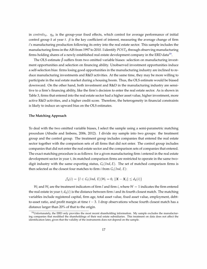
in controlsit. ηkt is the group-year fixed effects, which control for average performance of initialcontrol group k at year t. β is the key coefficient of interest, measuring the average change of firmi’s manufacturing production following its entry into the real estate sector. This sample includes themanufacturing firms in the AIS from 1997 to 2010. I identify POSTit through observing manufacturingfirms holding shares of a newly established real estate development company in the ERD data19.

The OLS estimate β suffers from two omitted variable biases: selection on manufacturing invest-ment opportunities and selection on financing ability. Unobserved investment opportunities inducea self-selection bias: firms losing good opportunities in the manufacturing industry are inclined to re-duce manufacturing investments and R&D activities. At the same time, they may be more willing toparticipate in the real estate market during a housing boom. Thus, the OLS estimate would be biaseddownward. On the other hand, both investment and R&D in the manufacturing industry are sensi-tive to a firm’s financing ability, like the firm’s decision to enter the real estate sector. As is shown inTable 3, firms that entered into the real estate sector had a higher asset value, higher investment, moreactive R&D activities, and a higher credit score. Therefore, the heterogeneity in financial constraintsis likely to induce an upward bias on the OLS estimates.

The Matching Approach

To deal with the two omitted variable biases, I select the sample using a semi-parametric matchingprocedure (Abadie and Imbens, 2006, 2012). I divide my sample into two groups: the treatmentgroup and the control group. The treatment group includes companies that entered the real estatesector together with the comparison sets of all firms that did not enter. The control group includescompanies that did not enter the real estate sector and the comparison sets of companies that entered.The exact matching procedure is as follows: for a given manufacturing firm i entered in the real estatedevelopment sector in year t, its matched comparison firms are restricted to operate in the same two-digit industry with the same exporting status, Gi(Ind, E). The set of matched comparison firms isthen selected as the closest four matches to firm i from Gi(Ind, E):

J4(i) = {l ∈ Gi(Ind, E)|Wl = 0, ‖X − X i‖ ≤ d4(i)}

Wl and Wi are the treatment indicators of firm l and firm i, where W = 1 indicates the firm enteredthe real estate in year t; d4(i) is the distance between firm i and its fourth closest match. The matchingvariables include registered capital, firm age, total asset value, fixed asset value, employment, debt-to-asset ratio, and profit margin at time t− 3. I drop observations whose fourth closest match has adistance larger than 20% of that to the origin.

19Unfortunately, the ERD only provides the most recent shareholding information. My sample excludes the manufactur-ing companies that modified the shareholdings of their real estate subsidiaries. This treatment on data does not affect theidentification later, given that the validity of the instruments does not depend on the sample.

17

Firm i’s potential outcome in year t is computed as:

Yi(0) =

Yi if Wi = 014 ∑i∈J4(i) Yj if Wi = 1

Yi(1) =

14 ∑i∈J4(i) Yj if Wi = 0

Yi if Wi = 1

Figure 3 plots the average R&D intensity, investment rate, and labor productivity of the twogroups around the time when firms in the treatment group entered the real estate development in-dustry. Time trends are taken out by controlling for year-specific effects.

Figure 3: The Effects of Entering the Real Estate Sector

Prior to entering the real estate sector, the treatment and control groups have similar trends inR&D intensity, investment rate, and labor productivity. After treatment firms participated in realestate activities, I observe a sharp decline in production in their original manufacturing businesses.

18

I next apply an instrumental variable approach to provide additional and robust evidence aboutthe causal effect of entering the real estate sector on manufacturing firms’ original businesses.

The Instrumental Variable Approach

I introduce an instrument for firms’ decisions to enter the real estate sector by exploring city-levelland supply elasticity and entrepreneurs’ potential connections with the local land bureaus. The landsupply elasticity is related to land appreciation during the construction period such that it predictsthe return in the real estate sector in a given city. The entrepreneurs’ potential connections with thelocal land bureaus exploit the institutional background in China, given corruptive behaviors in theland market.

I manually construct a land supply elasticity index20 for 145 cities following Saiz (2010), who char-acterizes the supply-side response to housing demand shocks. A city with a land supply elasticityindex of 1 implies that all areas within 30 kilometers of the city center can be developed into residen-tial or commercial properties. Column (1) in Table 5 tests the correlation between residential homeprice appreciations and the land supply elasticity index. When national house prices appreciate by100%, a city with 1% lower land supply elasticity would have a 0.78% faster three-year house pricegrowth. The corresponding estimate with 2-year lagged land prices21 being controlled for is 0.84%,which indicates that the land supply elasticity index can predict returns in the real estate sector. In ad-dition, as discussed in section 2, most real estate companies are restricted to operating locally exceptfor the less than 2% firms with an A-class license. Therefore, I consider the local real estate marketreturn as a key determinant for manufacturing firms’ decision to enter the real estate sector22.


The city land supply elasticity however has a low predictive power for individual firms’ decisionsto enter the real estate sector. The local land supply is in general constrained. From 2005 to 2015, anaverage of 6,713 pieces of land were sold per year, but there are a total of 83,913 real estate devel-opment companies on average23. Assuming a standard development period of two years, over 80%of the real estate companies could not always have a real estate project in development. To ensure astrong first stage in the IV analysis, it is necessary to find a firm-level variable that is correlated withthe decision of entering the real estate sector.

The firm-level variable is the potential connection between the CEO and local land bureau minis-ters. I defined the potential connection between the CEO of a firm and the local land bureau minister

20The index is normalized to a 0 to 1 scale.21Deng, Gyourko, Wu (2015) documents that the average period of housing development is two years and that the construc-

tion costs in China remained almost constant during the housing boom.22In data, I also found almost no manufacturing companies starting a real estate firm in other cities.23The numbers are calculated based on the CREIS statistics.

19

as whether or not they grew up in the same county. The ERD contains the first six digits of the nationalidentification number of CEOs, which indicate their home county at the age of 16. The birthplacesof local land bureau ministers are collected manually based on their official resumes. This variable isinspired by the literature on the impact of social networks on investment (Shue, 2013; Haselmann etal., 2016), but avoids the endogeneity concern in the formation of social networks. Given that mostland bureaus were established after 2004 and that a random sample from the ERD suggested thatfewer than 0.5% firms changed their CEOs, the potential connection variable is arguably not affectedby the investment opportunities of firms.

Figure 4 illustrates the significance of the land supply elasticity and the CEO’s potential connec-tion with local land bureaus in predicting entry to the real estate sector. I divide the manufacturingfirms into four groups based on their connections with the local land bureau and whether their homecity has an elastic land supply. I then plot the fraction of firms that entered the real estate sector ineach group. Over time, the group of firms with local connections and inelastic city-level land sup-ply is significantly more likely to participate in real estate development, compared to all other threegroups.

Figure 4: The Predictive Power of the Two Variables

In further examination, the land supply elasticity and the CEO’s potential connection with localland bureaus also significantly predict local land supply. I discuss related details in Appendix B.

20

The Identification Strategy

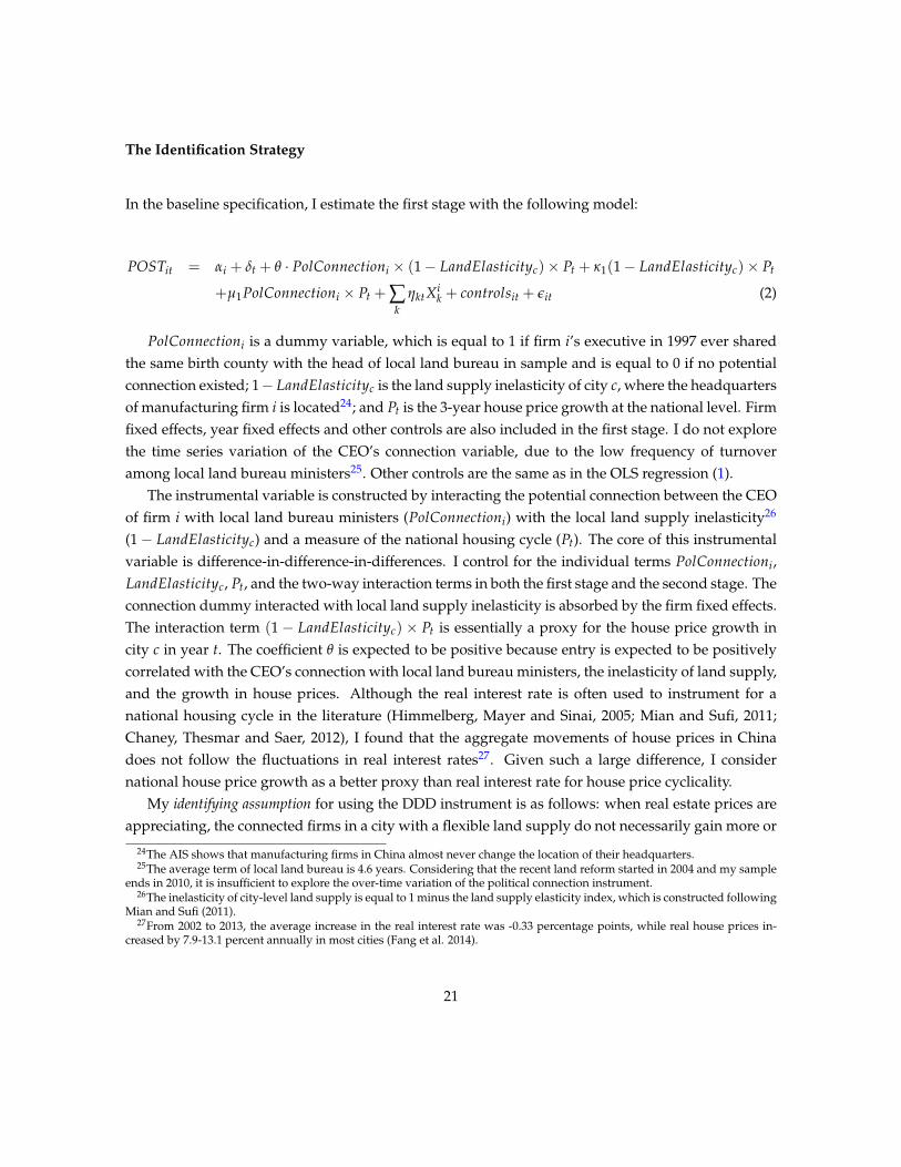
In the baseline specification, I estimate the first stage with the following model:

POSTit = αi + δt + θ · PolConnectioni × (1− LandElasticityc)× Pt + κ1(1− LandElasticityc)× Pt

+µ1PolConnectioni × Pt + ∑k


PolConnectioni is a dummy variable, which is equal to 1 if firm i’s executive in 1997 ever sharedthe same birth county with the head of local land bureau in sample and is equal to 0 if no potentialconnection existed; 1− LandElasticityc is the land supply inelasticity of city c, where the headquartersof manufacturing firm i is located24; and Pt is the 3-year house price growth at the national level. Firmfixed effects, year fixed effects and other controls are also included in the first stage. I do not explorethe time series variation of the CEO’s connection variable, due to the low frequency of turnoveramong local land bureau ministers25. Other controls are the same as in the OLS regression (1).

The instrumental variable is constructed by interacting the potential connection between the CEOof firm i with local land bureau ministers (PolConnectioni) with the local land supply inelasticity26

(1− LandElasticityc) and a measure of the national housing cycle (Pt). The core of this instrumentalvariable is difference-in-difference-in-differences. I control for the individual terms PolConnectioni,LandElasticityc, Pt, and the two-way interaction terms in both the first stage and the second stage. Theconnection dummy interacted with local land supply inelasticity is absorbed by the firm fixed effects.The interaction term (1− LandElasticityc) × Pt is essentially a proxy for the house price growth incity c in year t. The coefficient θ is expected to be positive because entry is expected to be positivelycorrelated with the CEO’s connection with local land bureau ministers, the inelasticity of land supply,and the growth in house prices. Although the real interest rate is often used to instrument for anational housing cycle in the literature (Himmelberg, Mayer and Sinai, 2005; Mian and Sufi, 2011;Chaney, Thesmar and Saer, 2012), I found that the aggregate movements of house prices in Chinadoes not follow the fluctuations in real interest rates27. Given such a large difference, I considernational house price growth as a better proxy than real interest rate for house price cyclicality.

My identifying assumption for using the DDD instrument is as follows: when real estate prices areappreciating, the connected firms in a city with a flexible land supply do not necessarily gain more or

24The AIS shows that manufacturing firms in China almost never change the location of their headquarters.25The average term of local land bureau is 4.6 years. Considering that the recent land reform started in 2004 and my sample

ends in 2010, it is insufficient to explore the over-time variation of the political connection instrument.26The inelasticity of city-level land supply is equal to 1 minus the land supply elasticity index, which is constructed following

Mian and Sufi (2011).27From 2002 to 2013, the average increase in the real interest rate was -0.33 percentage points, while real house prices in-

creased by 7.9-13.1 percent annually in most cities (Fang et al. 2014).

21

less advantage in manufacturing compares to a similar firm in a city with an inflexible land supply.The second stage is similar to the OLS specification, except that the two-way interaction terms are

controlled:

Yit = αi + δt + β · POSTit + κ2(1− LandElasticityc)× Pt

+µ2PolConnectioni × Pt + ∑k


For the robustness of the IV estimates, I also estimate the first stage, allowing year-specific re-sponses to the investment opportunity in the residential property market:

POSTit =αi + δt + θt · PolConnectioni × (−LandElasticityc) + κ1t(1− LandElasticityc)

+ µ1tPolConnectioni + ∑k

ηktXik + controlsit + εit

This specification controls for the heterogeneous effect of entry on a year-to-year basis, whichrequires no modeling of the aggregate housing cycle. The corresponding second-stage regression ismodified as:

Yit = αi + δt + β · POSTit + κ2t(1− LandElasticityc) + µ2tPolConnectioni + ∑k

ηktXik + controlsit + εit

In addition to the two linear specifications, I estimate the first stage non-parametrically by includ-ing in the second-order fractional polynomials of the two instruments and their interaction terms.Because adding the polynomial controls is equivalent to imposing multiple instruments, I conductthe Hausman overidentification test.

The Exclusion Restrictions

My key identification assumption is that when real estate prices are appreciating, the connected firmsin a city with a flexible land supply do not necessarily gain more or less advantage in manufacturingcompared to a similar firm in a city with an inflexible land supply. To test this exclusion restriction,I argue that the two instruments are uncorrelated with local economic trends, so that firms withdifferent exposures to them should not be subject to different aggregate shocks in the real estatebusiness cycle.

The land availability of a city is pre-determined by geographical constraints. Given the large

22

population in China and political considerations, cities are spread relatively evenly across the coun-try28. Table 6 presents the economic activities and spatial distribution of cities in four quartiles of theland supply elasticity measure. The cities in the four quartiles are distributed almost evenly acrosseconomic regions and different city-tier divisions, except that the east region has more cities in thea lowest land supply elasticity category. The average rates of population growth, GDP per capitagrowth, and employment growth are also very similar in the different quartiles. Columns (4) to (6)in Table 5 show that the city-level land supply elasticity interacted with national house price growthcannot significantly predict the growth rate of population, wages, and overall employment at thecity level29. Column (7) estimates the correlation between local export growth (measured as the ratioof the growth in total exports relative to total output) and land supply elasticity times the nationalhouse price growth. Controlling for city and industry fixed effects, the foreign demand for local man-ufacturing firms does not correlate with the instrumented local house price growth. Some inlandcities, which are non-export intensive and experience less economic development than their coastalcounterparts, also have a relatively inelastic supply of land due to geographical restrictions.


To show that local land supply elasticity does not correlate with housing demand, which mightaffect manufacturing demand via a substitution channel, I repeat the analysis in Davidoff (2016) bylooking at how the elasticity index can predict the quantity growth of newly constructed residentialproperties. The results are summarized in Table 7: a 1% higher land supply elasticity is associatedwith a 6.49 percentage points increase in the total floor space purchased per year. These estimatesstay statistically the same after controlling for local population growth and GDP per capita growth(in columns (2) and (3)), which implies that the land supply elasticity index does not correlate withshifts in the housing demand curve.


The potential connections between firm executives and local land bureau ministers are arguablyexogenous to economic trends by construction. Table 8 compares the performance of manufacturingfirms with and without a potential connection with the local land bureau between 1998-2002. Regard-less of city-specific constraints in land supply, firms with and without future connections were similarin size, productivity, investment rate, profit margin, credit score, and age prior to the real estate boom.

[Table 8 about here]28Figure A.1 in Appendix A provides an overview of the land supply elasticity index across China. Most cities that are short

of land are located on the east coast or or in the hilly areas in the west. The coastal region is considered the most economicallyactive in China, while the western region has the least growth potential.

29The local economic variables are computed with both SOEs and private firms in all industries.

23

However, there is not a single sufficient test for the exclusion restriction, given that the firm-specific investment opportunities are not observable to econometricians. In particular, I cannot con-clude that knowing the head of the local land bureau is completely independent from manufacturinginvestment opportunities. I argue that this possibility does not affect the validity of my proposedchannel. First, the supply of industrial land has not been a significant constraint on manufacturingproduction in China30. Cai et al. (2013) discusses that corruption mostly happens among residen-tial and commercial land auctions. Therefore, I consider the connection with local land bureaus ashaving little impact on manufacturing productivity. Second, knowing the head of the local land bu-reau is unlikely to be negatively correlated with the investment opportunities of firms. Therefore, myestimates at least indicate a lower bound of the causal effect. As a robustness check, I also controlfor firm-specific political connections with city mayors and vice-mayors, measured as whether or notthey share the same home county.

External Validity

The causal effects estimated using the instrumental variable approach are local average treatmenteffects (LATE). In a general framework, the relative return on real estate investment and the cost ofentry are two key factors determining if a manufacturing entrepreneur would enter the real estatesector. Therefore, the estimation of average treatment effect would require a random entry assign-ment that is independent of these two factors. In other words, the LATE estimate of this paper is theeffect of entry for firms with a connection with the local land bureau located in cities with constrainedland supply. If such relationships appear in land markets with higher return and lower entry cost,the IV specification estimates the causal effect with more weights on these land markets.

Main Results

Column (2) of Table 9 summarizes the OLS estimates using the sample of privately-owned firmsthat have been in operation since 1997. Following the establishment of a real estate developmentsubsidiary, manufacturing firms on average reduce their R&D expenditure by 0.0056 per RMB of totalassets; the average decline in capital spending is 0.042 per RMB of total assets; and labor productivityon average decreases by 6.4%. The effects on R&D intensity, investment rates, and labor productivityare equivalent to 7%, 25.4% and 5.2% of their respective standard deviation. Given that the accountingdata of the manufacturing firms and their real estate subsidiaries are documented separately, theeffect on labor productivity is unlikely to be driven only by the investment diversion into the realestate development industry.

30Typically, the value of industrial land is 5%-10% of the value of a residential land

24

Column (3) repeats the OLS analysis using firms that are selected using the nearest-neighbormatching estimator in Abadie and Imbens (2006, 2012). With the property development entrantsmatched to its similar non-entrants, the average effect of entry on labor productivity drops from6.4% to 3.83% and the drop in R&D intensity becomes 0.0106, which is nearly twice as much as thefull-sample estimates. The estimate of the coefficient of the investment rate changes the most. Theaverage reduction of firm-level investment rate is 0.125, as opposed to 0.042 when estimating with thefull sample. This is consistent with our previous conjecture: because labor productivity is more rele-vant to unobserved investment opportunity, the full-sample OLS estimates are likely to be downwardbiased. The bias in investment estimates depends on whether they are more sensitive to financial con-straints or the unobserved labor productivity.

Column (4) presents my instrumental variable estimation. The entry decision of manufacturingfirms is instrumented by local political connections to the land officials interacted with local land sup-ply elasticity. The baseline IV estimates are close to the results in column (3): entry to the real estatedevelopment industry results in a reduction of manufacturing R&D by 0.012 and investment by 0.15out of 1 RMB of total assets. This is equivalent to a 0.15 standard deviation drop in R&D intensity anda 0.95 standard deviation drop in the investment rate. In addition, average labor productivity of man-ufacturing firms also declines by 3.98% following entry. The first stage of the baseline specificationis reported in column (1). For a manufacturing firm that has connections with the local land bureau,a 1% increase in instrumented local house price growth would lead to a 0.15% higher probability toenter into the property development business. Column (5) adds controls of the current political con-nection with city mayors and vice-mayors. The estimates are slightly larger than the ones using thebaseline IV approach, but they are statistically indifferent.


The IV estimates using nonlinear first-stage controls are reported in Table 10. Panel A of Table 10reports the results of estimating heterogeneous year-specific responses to the real estate investmentopportunity. The propensity of manufacturing firms to enter the real estate industry increases overtime, except for 2008 when the Chinese economy underwent a severe slowdown. Panel B of Table 10reports the results of adding non-parametric controls into the first stage regressions. The estimatesare comparable with the baseline IV estimates, and the over-identification tests are not violated (witha p-value of 0.11). In the first stage, only the first- and second-order interaction terms are significant,so that the high-order controls do not impose many differences on the estimates.


Figure 5 provides the event study analyses on entering the real estate sector. No pre-trends aredetected in either outcome variable of interest.

25

Figure 5: The Event Study Plots

4 The Social Efficiency of Entrepreneurial Talent Allocation

In the previous section, I provide solid empirical evidence about entrepreneurial talent allocation ina real estate boom: richer, more talented manufacturing entrepreneurs divert their resources from themanufacturing sector to the real estate sector. This section provides a tractable two-period model torationalize the empirical findings and more importantly, to evaluate the efficiency of the observedentrepreneurial talent allocation in a real estate boom. The main purpose of this model is to assesswhether entrepreneurs enter the real estate sector following the criteria of a social planner.

There are three main features of the model: persistent and heterogeneous entrepreneurial talent,an imperfect financial market, and a minimum land requirement to enter the real estate sector. Thepersistence of entrepreneurial talent is crucial for the discussion of talent allocation. If entrepreneursface idiosyncratic productivity shocks but have the same talent distribution a priori31, the allocationof entrepreneurial talent will not generate implications on efficiency ex ante. The imperfect finan-

31This condition also includes the case where the talent of all entrepreneurs follow the same Markov Process.

26

cial market plays two important roles in this model: first, it governs the wealth accumulation ofentrepreneurs with different talents; second, it partially determines the allocation of entrepreneurialtalents in a real estate boom. Finally, the minimum land requirement in the real estate sector cre-ates a friction in entrepreneurs’ business choices. Only entrepreneurs who have accumulated enoughwealth in the first period can overcome the entry barrier created by the minimum land requirement.The entry barrier arises because of the scarcity of land. The entry barrier of the real estate sector istherefore increasing with land price. In a growing economy, the cost of land use increases with totaloutput. Therefore, industries using inflexible land as an input face a larger entry barrier compared toindustries that use a flexible input (capital).

For tractability, I assume that there are only two sectors in the economy: manufacturing and realestate. However, the results of the model can be generalized to an economy with multiple sectors andmultiple periods. For the rest of this section, I refer to the real estate sector as the housing sector fornotational purposes. A dynamic version of the model is discussed in Section 5.

4.1 Model Setup

The economy in the model consists of L workers and entrepreneurs with a measure of 1. Each en-trepreneur is indexed by their talent in the manufacturing sector zM ∈ [0, 1], which is drawn from acumulative distribution function F(zM).

The First PeriodIn the first period, all entrepreneurs operate in the manufacturing sector. This is to model the periodprior to the privatization of real estate construction32. Production in the manufacturing sector isconstant returns to scale and uses capital and labor as inputs:

y(zM, k, l) = (exp(zM)k)αMl1−αM

,

where 1 − αM is the labor share in the manufacturing sector and k and l are the capital and laborinput, respectively.

Each entrepreneur faces a borrowing constraint, which is modeled as a maximum leverage ratio ofλ. Therefore, for a given level of wealth a, the maximum capital input has to satisfy:

k ≤ λa, λ ≥ 1 (4)

The borrowing constraint assumption restricts the maximum of capital input of a firm to increasein entrepreneurs’ wealth. This assumption implies a positive correlation between wealth and en-

32In a more general setting, the model targets the entrepreneurs who operate in other industries prior to a real estate boom.Some of these entrepreneurs are reallocated into the real estate sector during the real estate boom. Therefore, it is reasonableto assume that they do not specialize in the real estate sector in the first stage.

27

trepreneurial talent, as shown in Table 3 and other work (Buera and Shin, 2013; Moll, 2014). It can bemicro-founded by the limited enforcement of borrowing contracts between entrepreneurs and banks(Townsend, 1979; Holmstrom and Tirole, 1998). Such a constraint implies that self-financing is theprimary mechanism for privately-owned firms to accumulate capital, which is well rooted in theliterature. Song et al. (2011) and Hsieh and Klenow (2009) show that Chinese private firms rely heav-ily on self-financing and receive only limited funding from banks and insignificant equity funding.Moreover, a maximum leverage ratio that is independent of capital prices shuts down an additionalinefficiency from capital prices fluctuations (Kiyotaki and Moore, 1997), so the discussion is morefocused on the allocation of entrepreneurial talents. By varying λ, I can trace out all degrees of effi-ciency in the financial market: λ = ∞ implies a perfect financial market, while λ = 1 indicates thatno firms can finance from external sources. The exact form of the borrowing constraint is not impor-tant here as long as the maximum investment is increasing in the entrepreneur’s initial wealth a andnon-decreasing in her talent z. I assume a constant λ across all groups for analytical convenience.

For simplicity, I further assume that all entrepreneurs have the same wealth a0 at the beginningof period 1. This assumption is to emphasize the importance of entrepreneurial talent on wealthaccumulation33.

The Second PeriodIn the second period, the economy experiences an unexpected real estate boom, and entrepreneurshave the option to enter the housing sector34. Production in the housing sector is also constant re-turns to scale. Due to the geographical constraint of land development, the total land supply in theeconomy is fixed at S.

Real estate developers use land and labor to produce housing:

h(zH , s, l) = (exp(zH)s)αHl1−αH

,

where 1− αH is the labor share in the housing sector and s, l are the land and labor input, respectively.The entrepreneurial talent in the housing sector is modeled as a reduced-form function of the

entrepreneurial talent in the manufacturing sector:

zH = c + bzM (5)

Equation (5) can be interpreted as the ex-ante correlation between entrepreneurs’ comparativeadvantage and their absolute advantage. This is a key extension from the literature, where in ex-

33In a more general setting, more talented entrepreneurs accumulate more wealth over time regardless of initial wealthdistributions. I also present evidence in section 3 that more productive private firms in China on average own more assets.Therefore, the assumption is not crucial but simplifies the two-period model.

34The main reason for modeling an unexpected real estate boom is to derive closed-form solutions for policy discussions.The efficiency argument will hold when agents anticipate the real estate boom and adjust their savings for the cost barrier inthe housing sector.

28

pectation b is typically assumed to be 1 (Midrigan and Xu, 2014; Buera, Kaboski, and Shin, 2012).Letting b = 1 is essentially assuming that all entrepreneurs have the same comparative advantageregardless of their talents in the manufacturing sector. Allowing b to differ from 1 generates hetero-geneous comparative advantages of different entrepreneurs. I later show that when b is smaller than1, entrepreneurs with higher talent in the manufacturing sector have both the absolute and the com-parative advantage in producing in the manufacturing sector, and thus should not enter the housingsector in a real estate boom; when b is higher than 1, the talented entrepreneurs in manufacturinghave the comparative advantage in the housing sector, although they are also more productive in themanufacturing sector.

Each entrepreneur is still subject to the maximum leverage ratio of λ, so the maximum capital andland input satisfy:

k + qs ≤ λ, λ ≥ 1, (6)

where q is the unit land price, which is taken as given for each entrepreneur.In addition, there is a minimum operating scale constraint in the housing sector. If an entrepreneur

were to operate in the housing sector, her land input has to be no lower than s.

s ≥ s or s = 0 (7)

This assumption intends to model the inflexible land input and also plays a role for the imperfect fi-nancial market to influence the allocation of entrepreneurs across the two sectors35. If there is no sucha constraint, i.e. s → 0, the borrowing constraint (5) only determines the land input of entrepreneursat the intensive margin, i.e. the scale of investment in the housing sector, but not at the extensivemargin.

The PreferenceBoth the representative worker and entrepreneurs in the economy consume manufacturing goods

only in the first period, and they consume both manufacturing goods and housing in the secondperiod (after the real estate liberalization). Given that the real estate boom is unexpected, the agentsmaximize their utilities in the first period without incorporating the housing sector. Therefore, theutility criteria is:

U1 = log c1 + β log c2,

where c1 is the consumption in the first period and c2 is the expected consumption in the secondperiod.

35This assumption corresponds to the cash deposit requirement in the Chinese land market

29

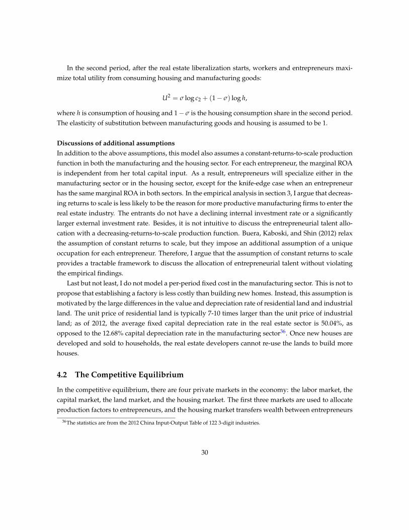
In the second period, after the real estate liberalization starts, workers and entrepreneurs maxi-mize total utility from consuming housing and manufacturing goods:

U2 = σ log c2 + (1− σ) log h,

where h is consumption of housing and 1− σ is the housing consumption share in the second period.The elasticity of substitution between manufacturing goods and housing is assumed to be 1.

Discussions of additional assumptionsIn addition to the above assumptions, this model also assumes a constant-returns-to-scale productionfunction in both the manufacturing and the housing sector. For each entrepreneur, the marginal ROAis independent from her total capital input. As a result, entrepreneurs will specialize either in themanufacturing sector or in the housing sector, except for the knife-edge case when an entrepreneurhas the same marginal ROA in both sectors. In the empirical analysis in section 3, I argue that decreas-ing returns to scale is less likely to be the reason for more productive manufacturing firms to enter thereal estate industry. The entrants do not have a declining internal investment rate or a significantlylarger external investment rate. Besides, it is not intuitive to discuss the entrepreneurial talent allo-cation with a decreasing-returns-to-scale production function. Buera, Kaboski, and Shin (2012) relaxthe assumption of constant returns to scale, but they impose an additional assumption of a uniqueoccupation for each entrepreneur. Therefore, I argue that the assumption of constant returns to scaleprovides a tractable framework to discuss the allocation of entrepreneurial talent without violatingthe empirical findings.

Last but not least, I do not model a per-period fixed cost in the manufacturing sector. This is not topropose that establishing a factory is less costly than building new homes. Instead, this assumption ismotivated by the large differences in the value and depreciation rate of residential land and industrialland. The unit price of residential land is typically 7-10 times larger than the unit price of industrialland; as of 2012, the average fixed capital depreciation rate in the real estate sector is 50.04%, asopposed to the 12.68% capital depreciation rate in the manufacturing sector36. Once new houses aredeveloped and sold to households, the real estate developers cannot re-use the lands to build morehouses.

4.2 The Competitive Equilibrium

In the competitive equilibrium, there are four private markets in the economy: the labor market, thecapital market, the land market, and the housing market. The first three markets are used to allocateproduction factors to entrepreneurs, and the housing market transfers wealth between entrepreneurs

36The statistics are from the 2012 China Input-Output Table of 122 3-digit industries.

30

and workers. Each agent takes prices in the four markets as given to maximizes their total utility. Inext discuss the entrepreneurs’ problems and the representative worker’s problem in detail.

The Entrepreneurs’ ProblemsIn the first period, the entrepreneur with talent zM makes decisions on consumption and savings inorder to maximize her total utility in the two periods:

maxa1(zM)

U1(zM) = log c1(zM) + β log c2(zM)

s.t. c1(zM) + a1(zM) ≤ Γ(λ, w1, R1, exp(zM)) · a0 (8)

c2(zM) ≤ Γ(λ, w2, R2, exp(zM)) · a1(zM), (9)

where w1 and w2 are the real wage in the first and the second period, respectively; and R1 and R2

are the cost of capital in first and the second period. The two budget constraints (8) and (9) areobtained by solving the profit-maximization problem of entrepreneur zM. In period t(t = 1, 2), giveninitial wealth at−1(zM), entrepreneur zM optimizes on labor and capital input subject to a borrowingconstraint in the capital market:

maxk(zM),l(zM)

[exp(zM)k(zM)]αM

l(zM)1−αM − wtl(zM)− Rt[k(zM)− at−1(zM)]

s.t. k(zM) ≤ λat−1(zM)

Lemma 1:The entrepreneurs’ wealth at the end of the first period, a1(zM) , is non-decreasing in zM.

(Proofs are provided in Appendix C). Lemma 1 is the result of the self-financing mechanism37: giventhe initial wealth, entrepreneurs with a higher talent in the manufacturing sector grow at a fasterspeed.

In the second period, when a real estate boom begins, the entrepreneur zM faces the option tooperate in the housing sector. Denoting pH and q as the house price and land price in period 2, theprofit-maximizing problem of entrepreneur zM then becomes:

37The self-financing mechanism can be easily generalized into a model with infinite horizons: in a world without the financialfrictions, only the most productive entrepreneur will participate in manufacturing production. However, when there is a max-imum leverage ratio and the initial wealth of entrepreneurs is not too dispersed, firms with heterogeneous productivity wouldco-exist in the market. Although productive entrepreneurs can generate a higher return than unproductive entrepreneurs, itsgrowth in each period is limited by the maximum borrowing constraint. Over time, the productive entrepreneurs occupy alarger and larger wealth share and eventually produce for all agents in the economy.

31

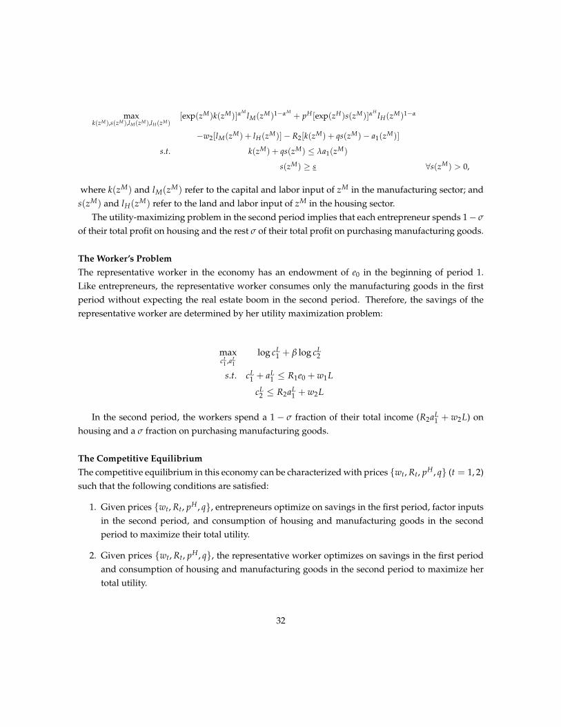
maxk(zM),s(zM),lM(zM),lH(zM)

[exp(zM)k(zM)]αM

lM(zM)1−αM+ pH [exp(zH)s(zM)]α

HlH(zM)1−α

−w2[lM(zM) + lH(zM)]− R2[k(zM) + qs(zM)− a1(zM)]

s.t. k(zM) + qs(zM) ≤ λa1(zM)

s(zM) ≥ s ∀s(zM) > 0,

where k(zM) and lM(zM) refer to the capital and labor input of zM in the manufacturing sector; ands(zM) and lH(zM) refer to the land and labor input of zM in the housing sector.

The utility-maximizing problem in the second period implies that each entrepreneur spends 1− σ

of their total profit on housing and the rest σ of their total profit on purchasing manufacturing goods.

The Worker’s ProblemThe representative worker in the economy has an endowment of e0 in the beginning of period 1.Like entrepreneurs, the representative worker consumes only the manufacturing goods in the firstperiod without expecting the real estate boom in the second period. Therefore, the savings of therepresentative worker are determined by her utility maximization problem:

maxcL

1 ,aL1

log cL1 + β log cL

2

s.t. cL1 + aL

1 ≤ R1e0 + w1L

cL2 ≤ R2aL

1 + w2L

In the second period, the workers spend a 1− σ fraction of their total income (R2aL1 + w2L) on

housing and a σ fraction on purchasing manufacturing goods.

The Competitive EquilibriumThe competitive equilibrium in this economy can be characterized with prices {wt, Rt, pH , q} (t = 1, 2)such that the following conditions are satisfied:

1. Given prices {wt, Rt, pH , q}, entrepreneurs optimize on savings in the first period, factor inputsin the second period, and consumption of housing and manufacturing goods in the secondperiod to maximize their total utility.

2. Given prices {wt, Rt, pH , q}, the representative worker optimizes on savings in the first periodand consumption of housing and manufacturing goods in the second period to maximize hertotal utility.

32

3. The labor market clears in the both periods, such that the total labor input in the economy isequal to L.

4. The capital market clears in both periods. Savers in the capital market include workers andentrepreneurs who have a return on capital lower than Rt; borrowers in the capital market areentrepreneurs who have a return on capital higher than Rt.

5. The land market clears in the second period. The total land used in production in the housingsector is equal to the exogenous land supply S.

6. The housing market clears in the second period. The total supply of housing is equal to the totalhousing demand of entrepreneurs and workers.

Proposition 1:There exists a unique competitive equilibrium in the economy. When the initial endowment of the representativeworker is large enough, the allocation of entrepreneurial talent in the real estate boom can be characterized asfollows:

a) If b ≥ 1, there exists two cutoffs zM and zMh , such that entrepreneurs with talent zM ∈ (zM, zM

h ] operatein the manufacturing sector; entrepreneurs with talent zM ∈ (zM

h , 1] operate in the housing sector; andentrepreneurs with talent zM ∈ [0, zM] exit and only save in the capital market.

b) If b < 1, the allocation of entrepreneurial talents can be characterized with three cutoffs: zM, zMl and zM

h .Entrepreneurs with talent zM ∈ (zM, zM

l ]⋃(zM

h , 1] operate in the manufacturing sector; entrepreneurswith talent zM ∈ (zM

l , zMh ] operate in the housing sector; and entrepreneurs with talent zM ∈ [0, zM]

exit and only save in the capital market.

The structural parameter b pins down the structure of comparative advantage38. When b > 1, en-trepreneurs’ comparative advantages in the housing sector, zH − zM, are increasing in their manufac-turing talents zM. In other words, entrepreneurs with higher talents in the manufacturing sector haverelatively higher returns to capital in the housing sector. Given prices, the talented manufacturing en-trepreneurs should specialize in housing in the second period, leaving two cutoffs for characterizingthe equilibrium: zM as determining whether or not to produce and zM

h as determining the businesschoice. On the other hand, when b < 1, entrepreneurs’ comparative advantages in the housing sectorare decreasing in their manufacturing talents zM. However given the entry barrier in the housing sec-tor, entrepreneurs with low zM’s are not able to accumulate enough wealth to enter the housing sector.As a result, entrepreneurs with talent zM ∈ (zM, zM

l ] could not follow their comparative advantagein producing housing.

38A detailed discussion of the comparative advantage will be provided in section 4.3.

33

4.3 The Social Planner’s Problem

This section examines whether the entrepreneurial talent allocation in the competitive equilibriumis constrained efficient. In doing so, I assume that the social planner faces the same constraints asindividual entrepreneurs: the individual borrowing constraint and the minimum operating scaleconstraint in the real estate sector. In other words, the social planner cannot arbitrarily assign pro-duction factors to entrepreneurs. Given that the real estate boom is unanticipated and that all agentsin the economy have the same utility function, the social planner solves the first period as what en-trepreneurs and workers achieve in a competitive equilibrium. This is a result implied by the secondwelfare theorem.

In the second period, I write the social planner’s objective function following Gorman’s Aggrega-tion Theorem:

U = χ log C + log H,

where C is the total consumption of entrepreneurs and workers and H is the total housing consump-tion in the economy. χ = σ

1−σ is the Pareto weight that corresponds to the competitive equilibrium.I first define the comparative advantage in the planner’s problem. As discussed in Proposition 1,

the entry barrier in the housing sector is the key constraint at the extensive margin. Entrepreneurswithout enough wealth cannot achieve the minimum scale in the real estate sector. The comparativeadvantage is defined as the allocation criteria followed by a social planner, assuming that there is noconstraint at the extensive margin.

Definition of Comparative Advantage:The comparative advantage of an entrepreneur is defined as the ratio of the marginal returns on capital in thetwo sectors. With a monotonic transformation, it is equivalent to zH − zM.

The difference between the social planner’s constrained optimization problem and a competitiveequilibrium is that the social planner is aware that land prices are a function of the allocation ofentrepreneurs. In the social planner’s problem, there also exists the private markets for land, capital,labor, and housing. Solving the social planner’s problem is thus equivalent to solving for the cutoffsdescribed in Proposition 1.

In the first case, when b > 1, entrepreneurs with a higher talent in manufacturing have the com-parative advantage in the housing sector. The social planner solves for the cutoff for producing, zM,and the cutoff for entering the housing sector zM

h :

34

max{zM ,zM

h ,l(zM)}χ log C + log H

s.t. C =∫ zM

hzM [exp(zM)k(zM)]α

Ml(zM)1−αM

dF(zM) (10)

H =∫ 1

zMh[exp(zH)s(zM)]α

Hl(zM)1−αH

dF(zM) (11)

λ∫ zM

hzM a1(zM)dF(zM) =

∫ 10 a1(zM)dF(zM) + aL

1 (12)

λa1(zMh ) ≥

λ∫ 1

zMh

a1(zM)dF(zM)

S s (13)∫ 1zM l(zM)dF(zM) = L (14)

In this problem, equations (10), (11), (12) and (14) refer to the resource constraints on the goodsmarket, housing market, capital market, and labor market, respectively. The constraint (13) combines

the resource constraint on the land market and the minimum operating scale constraint.λ∫ 1

zMh

a1(zM)dF(zM)

Sis the effective land price in this social planner’s problem.

In the second case, when b < 1, entrepreneurs with a lower talent in manufacturing have thecomparative advantage in the housing sector. The social planner solves for three thresholds: one forproducing, zM, and two for operating in the housing sector: zM

l , zMh . The social planner’s problem

can be written as:

max{zM ,zM

l ,zMh ,l(zM)}

χ log C + log H

s.t. C =∫[zM ,zM

l )⋃(zM

h ,1][exp(zM)k(zM)]αM

l(zM)1−αMdF(zM) (15)

H =∫ zM

hzM

l[exp(zH)s(zM)]α

Hl(zM)1−αH

dF(zM) (16)

λ(∫[zM ,zM

l )⋃(zM

h ,1] a1(zM)dF(zM)) =∫ 1

0 a1(zM)dF(zM) + aL1 (µk) (17)

λa1(zMl ) ≥

λ∫ zM

hzMl

a1(zM)dF(zM)

S s (µe) (18)∫ 1zM l(zM)dF(zM) = L (µl) (19)

Similar to the first case, equations (15), (16), (17) and (19) refer to the resource constraints on thegoods market, housing market, capital market, and labor market, respectively. The constraint (18)combines the resource constraint on the land market and the minimum operating scale constraint.

35

Proposition 2:When the least talented manufacturer zM is constrained from entering the housing sector, the competitiveequilibrium is constrained efficient if and only if b ≥ 1. In the case when b < 1, both zM

l and zMh are higher in

the competitive equilibrium than in the social planner’s problem.The socially optimal allocation of entrepreneurs should be determined by their comparative ad-

vantages in the housing and the manufacturing sectors. Whether or not a financial market frictioncan distort the entrepreneurs’ choices at the extensive margin is then determined by the relationshipbetween entrepreneurs’ comparative advantages and their absolute advantages in the manufacturingsector. Panel (a) of Figure 6 illustrates an example of a positive correlation between the compara-tive advantage in the housing sector and the absolute advantage (talent) in the manufacturing sector,meaning that entrepreneurs with high zM’s should switch to the housing sector in the optimal situ-ation. In this case, the entry barrier in housing production does not impose additional distortions ofthe entrepreneurs’ allocation. The productive manufacturing entrepreneurs would have accumulatedenough wealth, so they are in fact unconstrained by the entry barrier in housing production.

Panel (b) of Figure 6 shows an opposite example, in which entrepreneurs with low zM’s shouldoperate in housing production in the optimal situation. The thresholds labeled with ”CE” refer tothe competitive equilibrium, and the thresholds labeled with ”SP” refer to the solution to the socialplanner’s problem. The entry barrier and financial market imperfection prevent these unproduc-tive manufacturing entrepreneurs from entering the real estate sector. According to the empiricalevidence provided in section 3, entrepreneurs entered the real estate sector have a higher talent inmanufacturing. However, when entrepreneur-specific financing ability is controlled, the pattern nolonger exists: unproductive manufacturing entrepreneurs are more likely to enter the real estate sec-tor. This empirical evidence suggests that the entrepreneurs’ comparative advantage is negativelycorrelated with their talent (absolute advantage) in the manufacturing sector, and that the financialmarket imperfection is distorting the allocation of entrepreneurs across sectors.

Two groups of entrepreneurs’ choices at the extensive margin are distorted. First, the entry bar-rier results in a lack of competition in the land market, which extracts monopolistic rents to the landowners. The monopolistic rents attract entrepreneurs with talent in (zM

h,SP, zMh,CE] to enter the hous-

ing sector. Given that the more talented manufacturing entrepreneurs also own more wealth, theland price is higher in the competitive equilibrium than in the planner’s problem. Therefore, a largerfraction of entrepreneurs who have a higher comparative advantage in housing are constrained fromentry. This group refers to entrepreneurs with talent in (zM

l,SP, zMl,CE]. Endogenizing land prices allows

the social planner to allocate entrepreneurs efficiently at the extensive margin. In section 5, I pro-vide more evidence on the negative correlation between comparative advantage in housing and theabsolution advantage in manufacturing.

36

Figure 6: The Entrepreneurs’ Business Choices

(a) b > 1

zM

MRKMRKH

MRKM

aMh,SP = aM

h,CE

(b) b < 1

zM

MRK

MRKH

MRKM

aMl,SP aM

l,CE aMh,SPaM

h,CE

4.4 Discussion of Policy Tools

In this section, I focus on the case when b < 1 and discuss three policy tools for improving socialwelfare: liberalizing the financial market, a more flexible schedule for land supply (or a reducedentry barrier), and taxation on the return on capital in the real estate sector.

The first two policy tools relax the borrowing constraint and the minimum operating scale con-straint, respectively. These changes not only apply to the competitive equilibrium but also relax theconstraints in the planner’s problem. As a result, financial market liberalization and increasing landsupply do not help with alleviating the inefficiency. The taxation on returns in the real estate sector,on the other hand, directly reduces the excess return due to the lack of entry, so that it partly solvesfor the inefficiency in the entrepreneurial talent allocation.

Financial market liberalization:A more liberalized financial market (a higher λ) increases zM and lowers zM

l and zMh , resulting in higher social

welfare but larger inefficiency at the extensive margin.In theory, a more liberalized financial market can be modeled as a marginal increase in the max-

imum leverage ratio λ. A higher λ is welfare-improving from two aspects. First, it directly reducesthe resource misallocation in the economy, given that more productive entrepreneurs are allowed toborrow more. Second, the constrained entrepreneurs who have the comparative advantage in thehousing sector are more capable of acquiring capital, so that they are more likely to overcome theentry barrier in the housing sector.

This result suggests that given existing constraints in the real estate sector, in a developed country

37

where the financial market is less imperfect, the social welfare is higher than in a developing economy.The finding is consistent with the literature, which argues that a more liberalized financial marketimproves resource misallocation. However, the inefficiency (the discrepancy between the competitiveequilibrium and the planner’s solution) at the extensive margin is exacerbated. The already wealthyentrepreneurs are now able to borrow more, which further increases the land prices. As a result,more entrepreneurs with low wealth (and therefore comparative advantages in the housing sector)are constrained by the entry barrier. A detailed proof is provided in Appendix C.

A lower cost barrier to entry:A smaller entry barrier in the real estate sector (a smaller s

S ) lowers zM, zMl , zM

h , and lowers inefficiency at theextensive margin. The welfare consequence is ambiguous.

An increase in land supply in the model is equivalent to a decline in the minimum operatingscale, which effectively lowers s

S . This policy directly targets the origin of the social inefficiency, sothat entrepreneurs are less constrained by the entry barrier in the real estate sector. In reality, theflexibility of land supply is often subject to geographical or political constraints. Lowering the entrybarrier in the real estate market has an ambiguous impact on aggregate welfare. Despite the fact thatthe minimum operating scale in the real estate sector is lower, there are more entries in the real estatesector. Unproductive entrepreneurs, who might have become savers when the entry barrier is large,now produce actively. The aggregate productivity is thus lower.

Taxation on the return from property sales (the stamp duty):Taxing the returns from real estate development lowers zM, zM

l and zMh , resulting in a higher social welfare and

a lower inefficiency at the extensive margin.This policy tool is equivalent to imposing a wedge on the returns from selling houses. Instead of

obtaining pH from selling one unit of housing, the real estate developers now get pH(1− τ). Tax-ing the returns on the real estate market do not change the planner’s problem. It is also an effectivepolicy because it lowers the return from producing in the real estate sector, so the more talentedentrepreneurs in the manufacturing sector lose the incentive to enter. Due to the lack of entry ofwealthy entrepreneurs, the land price is also lower so fewer entrepreneurs with a comparative ad-vantage in housing are constrained from entry. In summary, this policy tool deals with both groupsof entrepreneurs who were inefficiently allocated in the original competitive equilibrium by correct-ing their incentives.

5 Quantitative Evaluation

For the quantitative evaluation, I generalize the two-period model to a life-cycle model with overlap-ping generations. The economy consists of L workers and N groups of entrepreneurs. Each agent in

38

the economy works for 30 years and saves for 20 years after retiring39. While working, both work-ers and entrepreneurs can only save in the capital market. Young workers earn labor compensation,and young entrepreneurs earn manager compensation as a fraction of old entrepreneurs’ investmentreturn through managing their family firms. When agents retire, they can either save in the capitalmarket or old entrepreneurs can invest in their family firms. The technology and preferences are thesame as in the two-period model.

In each period, each old entrepreneur makes decisions on the capital investment into the familyfirm, while the young entrepreneur as the manager decides on the business choices of the company.Each family firm still faces the borrowing constraint and the minimum operating scale constraintin section 4. Therefore, both the entrepreneurial talent of the young manager and the firm-specificfinancing ability determines the business choice of each firm. I assume that there is no agency problembetween the old entrepreneurs and the managers of their family firms. Allowing entrepreneurs tosave in their family firms guarantees that entrepreneurs with different talent accumulate their wealthat different speeds. Therefore, the positive correlation between wealth and talent still holds in thelife-cycle model.

I first focus on the structural estimation of b using data on the manufacturing performance andreal estate performance of the same entrepreneur. From the discussions in section 4, b is the key pa-rameter that governs the relationship between the comparative advantage and absolute advantageof entrepreneurs. The allocation of entrepreneurial talent is inefficient when b < 1, which impliesproductivity manufacturing entrepreneurs are not more productive in the housing sector. The identi-fication of b then answers if the observed allocation of entrepreneurial talent is efficient or not in theChinese real estate boom.

Next, I calibrate the life-cycle model with overlapping generations using aggregate moments fromChina. In the literature, the entry barriers in industries are often calibrated using the average firm size.In my model, however, both the entry barrier and the structural parameter b govern the selection intoreal estate. Therefore, they cannot be jointly identified using the average firm size in the real estatesector. I take the estimated parameter b as given and calibrate the entry barrier s and other parametersof the model by matching empirical moments during 1997 to 2010, which corresponds to the coverageof my sample. Based on the calibration, I conduct policy counterfactuals that focus on the three policytools discussed in section 4.

5.1 Structural Estimation

I structurally estimate the parameter b, which governs the correlation between the comparative ad-vantage and the absolute advantage of entrepreneurs. In the data, entrepreneurs also face idiosyn-cratic productivity shocks. Estimating b at the firm level is not realistic and also subject to large

39The parametrization follows Song et al. (2011)

39

measurement errors. I follow the literature of comparative advantage (Hurst et al. 2013; Adao, 2015)by estimating b at a higher level. I divide entrepreneurs into groups according to their levels of edu-cation and work experience. Because my data covers only the first six years of the real estate boom,I consider the education and work experience of each manager as stable and pre-determined withinthis period. Studying the behavior of entrepreneurs across groups further alleviates the concern aboutthe constant-returns-to-scale assumption. In the model, although each entrepreneur only specializesin one sector, there is partial specialization at the group level, which matches the observation in thedata.

The talent of a given entrepreneur i in group g is assumed to satisfy the following structure:

zMit = zM

g + ξMt + ωit

zHit = zH

g + ξHt + εit

zHg = c + bzM

g

zMg and zH

g are constant group-average productivity in the manufacturing sector and the housingsector; (ξM

t , ξHt ) are aggregate productivity shocks to these sectors; and ωit, νit are idiosyncratic un-

expected productivity shocks40, which do not depend on group g. This structure of entrepreneurialtalents is designed to facilitate the identification of b, which is key to determining the efficiency oftalent allocation as discussed in Proposition 2.

The structural parameter b governs the correlation between the group-specific comparative ad-vantage and absolute advantage. When b > 1, the groups with an absolute advantage in the man-ufacturing sector should specialize more in the real estate sector in the event of a real estate boom;when b < 1, the groups with an absolute advantage in the manufacturing sector should stay in man-ufacturing.

I estimate the structural parameter b using a unique firm-level data set that matches manufactur-ing firms to their real estate subsidiaries. This is equivalent to matching the manufacturing businessand the real estate business of the same entrepreneur. The key structural parameter b cannot be iden-tified using a standard simulated method of moments approach, as usual macro moments (establish-ment scale) cannot distinguish b from the entry barrier s. In other works on misallocation and growthin a multi-sector economy, b is typically assumed to be 1. As a result, the average size of entrants pinsdown the entry barrier parameter. However, if b is not fixed, the size of entrants is determined byboth the entry barrier and the comparative advantage of the entrants. The micro-level data makes it

40In an economy with only idiosyncratic productivity shocks and with zg identical among entrepreneurs, there is also ineffi-cient allocation of talent in the presence of an incomplete financial market and a cost barrier to entry (Burea, Kaboski and Shin,2012). Adding the ex-ante heterogeneity of entrepreneurial talents, however, will likely to create a larger inefficiency (b < 1)or a smaller inefficiency (b > 1). The self-financing mechanism (as shown in Lemma 1) induces a positive correlation betweenwealth and entrepreneurial talent.

40

possible to jointly identify the comparative advantage of entrepreneurs and the entry barrier in thereal estate sector.

Data

The data used for the structural estimation are mainly from three sources: the AIS, the ERD, andthe 2008 Economic Census. The AIS is used to estimate the manufacturing production function andgroup specific average productivity. The ERD contains the shareholding information of all registeredbusinesses in China. Therefore, I can use the registration database to match manufacturing firms totheir real estate development subsidiaries. A detailed introduction of the two data sets is provided insection 3.1.

Given that the AIS only covers industrial firms, I collect the operation information of the real es-tate firms using the National Economic Census. There have been three national economic censuses,which were carried out in 2004, 2008, and 2013 respectively. Given that the housing market reformswere not yet completed by 2004 and that the micro-level data of the 2013 census is still not available,I use the cross section of the 2008 national economic census to estimate the production of real estatedevelopment firms. The second national economic census in 2008 covered over 7,099,000 enterprisesin China’s secondary and tertiary industries, including data about production, management, invest-ment, and corporate structure at the firm level. Table 1 provides a summary of the variables fromthe National Economic Census. In the Economic Census data, 1,299 real estate firms are found to besubsidiaries of manufacturing companies covered by the AIS.

The manager information is obtained from the ERD. I classified the managers into different groupsaccording to their levels of education and work experience, which are pre-determined and not influ-enced by any firm-specific shocks between 1995 and 2010. There are 20 groups based on five levels ofeducation and four quartiles of managers’ work experience. The five education levels include gradu-ate, undergraduate and post-high school, high school and vocational high school, middle school, andelementary school and below. The experience of managers varies from 1 to 48 years. I then divide themanagers into four quartiles based on their managing experience

Estimating the Structural Parameter

The structural estimation of b is equivalent to regressing the marginal return to capital in the realestate sector on the marginal return to capital in the manufacturing sector. As illustrated in Figure 2,the marginal return to capital in the real estate sector is labelled with red, and the marginal return tocapital in the manufacturing sector is labelled with blue. The regression is derived from the followingspecification, which is directly implied by the model:

41

logph

t hitkit− log πH

t = c + bzMg + ξH

t + εit, (20)

where πHt = ( 1−αH

wt)

1−αH

αH p1/αHtqt

and pht hitkit

is the average product of capital. I estimate the group-specifictalent in the manufacturing sector, zM

g , with firm-level data prior to the real estate boom.There are two key challenges for the estimation of b: first, the observed marginal return to capital

in the manufacturing sector has measurement error, which creates attenuation bias; and second, Ido not observe the real estate performance of entrepreneurs who did not enter the real estate sector,which induces selection bias. The selection bias leads to the error term (εit|Hg,t) not centering around0:

E(logph

t hitkit

) = const + bzMg + E(εit|(εit, ωit) ∈ Hg,t), (21)

where Hg,t indicates the group of entrepreneurs in group g that choose to enter the real estate sectorin year t.

The measurement error problem biases the estimate of b towards 0. The selection bias results inthe estimate of b being biased towards 1. When b > 1, more productive manufacturing entrepreneursshould specialize in the real estate sector. The probability of entry into the real estate sector is increas-ing in zM

g , so the correlation between E(εit|(εit, ωit) ∈ Hg,t) and zMg is negative. Therefore, the self-

selection of entrepreneurs induce a downward bias. When b < 1, more productive manufacturingentrepreneurs should specialize more in the manufacturing sector, so that the probability of entry intothe real estate sector is decreasing in zM

g . In this case, the correlation between E(εit|(εit, ωit) ∈ Hg,t)

and zMg becomes positive and the self-selection introduces an upward bias. In summary, the selection

bias would result in b to be biased towards 1.I correct for the attenuation bias using the Empirical Bayes approach, which is often used in the

literature for evaluating the value added from teachers (Kane and Staiger, 2008; Meghir and Rivkin,2011; Chetty, Friedman and Rockoff, 2014). As with the selection bias, I employ the non-parametricbias correction approach following Das, Newey, Vella (2003). The approach is similar to the Heckmantwo-step correction but does not require a normality assumption. The main idea of this approach isto proxy for the selection bias with a non-parametric function of the firm-specific propensity score forentering the real estate sector.

I conduct the estimation of b following a three-step procedure. In the first step, I estimate theaverage talent of each group of entrepreneurs as the average Solow residual, using data prior to 2002.During this period, the manufacturing entrepreneurs have little incentive or ability to enter the realestate development industry, so the estimation is not subject to selection bias. Second, I estimatethe entrepreneur-specific propensity score of entering the real estate industry. The city-specific landsupply elasticity and the entrepreneur’s potential connection with the local land minister are used as

42

instruments for correcting the selection bias. Finally, I plug in the Bayes-adjusted estimate of group-specific manufacturing talent to estimate equation (21). The selection bias, E(εit|(εit, ωit) ∈ Hg,t), isproxied with a non-parametric function of the propensity score of entry, as estimated in the secondstep.

Next I discuss the three-step identification procedure in detail.

Step 1: As discussed in section 2, the Chinese housing market was highly regulated on the thedemand side and the supply side in the 1990s. Prior to the 2002 land market reform, privately-ownedmanufacturing firms had neither the ability nor the incentive to enter into the property developmentindustry. Therefore, manufacturing entrepreneurs focused only on manufacturing production duringthe pre-boom era. I estimate the entrepreneurs’ talent in the manufacturing sector following Basu andFernald (1997)41 by estimating a residual from the production function:

1αM

Indi

log yit − log kit −1− αM

Indi

αMIndi

log lit = α0 + αg + δt + eit, (22)

where αMIndi

is the average capital share of the 4-digit industry to which entrepreneur i belongs andαg is an estimate of the group specific manufacturing talent, zM

g . To correct for the attenuation biasinduced by the measurement errors, I apply an empirical Bayes approach. The group-specific talent,zM

g , is assumed to be drawn from a higher-level distribution:

zMg ∼ G0(z0, σ2

0 ),

where z0 and σ20 are the mean and variance of the higher-level distribution. The estimated group-

specific talent, αg, then follows a lower-level distribution that is centered around zMg :

αg ∼ G1(zMg , σ2

1 ),

where σ21 represents the measurement error. The empirical Bayes estimate of zM

g is thus:

ˆzMg =

σ21

σ20 + σ2

1

z0 +σ2

0

σ20 + σ2

1

αg,

where z0 is estimated as the constant α0 from regression (22); σ20 + σ2

1 is estimated as the variance ofαg, and σ2

1 is estimated as the average within-group variance of each αg.The estimation is conducted with the unbalanced sample of firms from 1997 to 2002.

41The estimation in this paper is a simplified version of Basu and Fernald (1997). First, I assume that the markets are perfectlycompetitive so the markups in both the manufacturing and housing sector are equal to 1. Second, I assume that entrepreneursproduce with only capital and labor so the factor shares for value added is the same as the factor shares for total output.

43

Step 2: The purpose of the second step is to estimate the propensity of entrepreneur i (firm i) enter-ing the real estate sector, i.e. P((εit, ωit) ∈ Hg,t). Due to data availability, I could not observe a dy-namic panel for the real estate development firms. Therefore, the propensity score is estimated as theprobability of entering into the real estate industry between 2004 and 2008, using a semi-parametricspecification:

Entryi,2008 = γ0 + γ1 log wc,2004 + γ2 log pc,2008 + γ3 log qc,2004 + F( ˆzMg , ai,2004, CreditScorei,2004)

, where F(zMg , ai,2004, CreditScorei,2004) is a fractional polynomial function of ˆzM

g , firm i’s total assetvalue in 2004 – ai,2004, firm i’s credit score in 2004, and their interaction terms. The fitted value

ˆEntryi,2008 ≡ Pi is the estimated propensity score for entry.

Step 3: The last step estimates b and tests the structural relationship between b and 1. The identi-fying assumption is that conditional on ˆzM

g and other factors used to estimate the propensity score ofentry, the unobserved εit is orthogonal to zM

g42:

E(εit|(εit, ωit) ∈ Hg,t, wt, pt, qt, ait, ˆzMg , Pi) = 0

With the identifying assumption, the selection bias can be corrected with a non-parametric speci-fication of the estimated propensity score43:

logpH

t hiki

= αc + b( ˆzMg ) + Λ(Pi) + εit,

where t is the year of 2008; αc is city fixed effect to control for local prices in city c; Λ(Pi) is a fractionalpolynomial function of the estimated propensity score Pi, which works as a proxy for the selectionbias E(εit|(εit, ωit) ∈ Hg,t); and b is a consistent estimator of b, so the test of an efficient allocation ofentrepreneurial talent is equivalent to testing the null hypothesis of H0 : b > 1. Following the litera-ture of control functions (Wooldridge, 2007), I conduct the statistical inference based on bootstrappingthe sample at the manager level.

42The methodology would still work if we generalize zHi to be a time-varying Markov process: zH

it = f (zHi,t−1) + εit. In this

case, the identifying assumption is valid as long as managers make their occupation choices for period t before zHit is realized.

The non-parametric propensity score controls for the variation in zHi,t−1 that can be explained by zM

g . The remaining component, together with unexpected shocks εit and εit, would still be orthogonal to zM

g .43A proof and related discussion can be found in Das, Newey and Vella (2003).

44

Main Results

I first provide raw patterns from data that suggest b < 1, i.e. the entrepreneurs with the absoluteadvantage in the manufacturing sector do not also have a comparative advantage in the real estatesector. Figure 744 plots the average return to capital in the two sectors against the entrepreneurs’talent in manufacturing as estimated in step 1.

Figure 7: Average Return to Capital in Two Sectors

Table 11 summarizes the estimation results from the three-step approach. Columns (1) to (3) re-port the coefficients estimated with firm-specific talent, group-specific talent, and the group-leveltalent adjusted with the Empirical Bayes approach. Given the bias induced by the measurement er-rors, columns (1) and (2) are subject to attenuation bias. The null hypothesis of b ≥ 1 is rejected byall three estimations, indicating that there is likely a negative correlation between the comparativeadvantage in real estate and the absolute advantage in manufacturing. This supports the observationthat allocation of entrepreneurial talent in the Chinese real estate boom is constrained inefficient.

[Table 11 about here]44This figure is generated using the “binscatter” function in Stata.

45

5.2 Calibration and Counterfactual Policy Analyses

The calibration is based on the extended life-cycle model with overlapping generations. Given that aseries of deregulations led to the real estate boom in China, I consider them as permanent shocks. Myprimary interest is to calibrate an economy transitioning to a new balanced growth path. The valuefunction of each agent then depends on the entire path of prices, including wage, interest rate, houseprice, and land price. The set of state variables contain talent (zM

it , zHit ), wealth, age, and year. To sim-

plify the computation process, I calibrate the entrepreneurs’ decisions at the group level and assumethat (εit, ωit) are zero. In doing so, I replace the state variable (zM

it , zHit ) with exogenously fixed av-

erage productivity (zMg , zH

g ). The talent distribution of group-specific talent, zMg , follows a truncated

Zeta distribution, which is a discrete approximate to the Pareto distribution. The probability densityfunction of zM

g is:

Pr(zMg ) =

1/gζ

∑Ni=1 1/iζ

, ζ > 1

The total asset value available for each firm is determined by the old entrepreneurs’ savings de-cisions. I further assume that the market for hiring young entrepreneurs as managers is competitive.Given that prior to the housing boom the group with a higher zM

g faces a larger return of capital, themanager compensation is increasing in g. The expected wage of each group mg,t is determined suchthat the incentive compatibility constraint for each young entrepreneur is binding. The parameterdetermining the manager’s compensation is assumed to be ψ, which is the minimum fraction of cap-ital return that managers can steal. The size of ψ determines the overall growth rate of the economy.When ψ is higher, the income dispersion is larger in younger generations so the group of productivefirms in manufacturing accumulate wealth at a faster speed.

To more closely model the Chinese economy, I add the SOEs in my quantitative analysis. Follow-ing Song et al. (2011), I assume that the SOEs are neither financially constrained nor managed by anyentrepreneurs. Their role in the model is to clear the capital market in early years, when entrepreneurshave not accumulated enough wealth. The productivity of SOEs is assumed to be κ fraction of theaverage productivity of privately-owned firms.

There are two stages in the calibration. The first stage, the pre-boom stage, corresponds to the firstperiod in section 4. The second stage models the real estate boom. I consider the real estate boom asdriven by a permanent preference shock, such that agents increase the housing consumption sharefrom 0 to ρ. I estimate parameters on manufacturing talent distribution, manager compensation,and initial wealth using in the first stage and parameters that determine average housing talent andentry barrier in the second stage. The rest of the parameters are set exogenously. Table 12 provides adescription for the exogenously determined parameters.

46

Table 12: Exogenously Determined Parameters

Parameter Description Value Sourceβ The utility discount factor 0.99 Song et al. (2011)λ Maximum leverage ratio 1.35 Buera ans Shin (2013)N Total groups of entrepreneurs 5 Education levels in data

αM Capital input share in manufacturing 0.5Bai, Hsieh, and Qian (2006),

Song et al. (2011)αH Capital input share in housing 0.85 China input-output tableb Comparative advantage parameter - 0.21 Point estimates from section 5.1

δM Capital depreciation rate inmanufacturing 0.1 Song et al. (2011)

δH Land depreciation rate in housing 0.5 2-year construction periodT1 Working age for workers and entrepreneurs 30 Song et al. (2011)T2 The number of year retiring 20 Song et al. (2011)

I assume that the first stage starts from 1992 (following the assumption in Song et al., 2011) andlasts for 10 years, until the 2002 land market liberalization. I calibrate the talent distribution usingthe estimated firm-level productivity between 1997 to 2002. Given the shape parameter ζ = 2, thedistance parameter is estimated to be dM = 0.15. I set SOE productivity κ = 0.397 to match the rela-tive capital-to-output ratio of SOEs and private companies, 2.65. Last but not least, the initial wealthof workers and entrepreneurs is calibrated such that the average share of total fixed assets of privatecompanies during 1997-2002 is close to 31.75% as in my data. The initial life-cycle distribution ofwealth for entrepreneurs and workers is similar to a scaled-up version of the distribution of wealthover the life cycle in the balanced growth paths. Entrepreneurs with different talent groups are as-sumed to start with the same wealth level. The minimum fraction of capital return a manager cansteal (ψ) is estimated as 0.2, which matches the growth rate of the average share of total fixed assetsowned by private companies. The model-based share in 1992 is 17.36%, which is close to 15.12% inthe data.

In the second period, I take the wealth distribution in 2002 as the initial wealth and calibratethree parameters: s, c, and housing consumption share ρ. I calibrate the housing consumption shareρ = 0.4. Assuming an average worker works for 30 years, this yields a price-to-income ratio of10.41, which matches the average price-to-income ratio of 10.2 in the data. Based on the proofs inappendix C, the entry decisions of entrepreneurs do not depend on the average productivity in realestate. Therefore, I calibrate the entry barrier using the average difference in log productivity betweenentrepreneurs who entered the real estate sector and others who did not. In the data, the averagedifference is estimated to be 0.25. This leaves me with an estimate of s = 0.046. I interpret the estimateas follows: in an average city in China, the average startup cost for a real estate project is 4.6% of the

47

total value of land supplied in the city. The parameter c indicates the average log productivity in thehousing sector. I estimate c to match the relative firm size in the manufacturing sector and the realestate sector. In the data, an average manufacturing firm hires 7.54 times more employees than anaverage real estate development firm. The average housing talent c is then estimated to be 0.31. Table13 summarizes the calibrated parameters and corresponding moments in the data.

Table 13: Calibrated Parameters

Target Moments Data Model Parameter Description

Variance of group-level log productivity 0.022 0.022 ζ = 6.07Scale parameter formanufacturing talent

Relative K/Y of SOEs and private firms 2.65 2.38 κ = 0.397 SOE productivityGrowth rate of private capital share 7.87% 8.89% ψ = 0.20 Manager IC parameterShare of capital held by private firms 31.75% 35.44% Initial wealthHouse price to income ratio 10.2 10.41 ρ = 0.40 Housing consumption share

The difference in manufacturing productivitybetween real estate entrants and other firms

0.25 0.23sS= 0.046 Entry barrier in real estate

Relative scale in manufacturing and real estate 8.54 8.06 c = 0.31 Average housing productivity

Panels A-C of Figure 8 compare several macroeconomic outcomes of the model and data. Themost important prediction of this model is on the relative growth rate of land prices to house prices.In early years of the real estate boom, the large preference shock induces a high return from operat-ing in the real estate sector. The unproductive and poor manufacturing entrepreneurs, who have thecomparative advantage in real estate, are initially constrained from participating in the land market.In order to attract the productive and talented manufacturing entrepreneurs, the land price must below enough so their ROA in real estate is higher than their ROA in manufacturing. As entrepreneursaccumulate wealth at a different speed, over time real estate entrepreneurs with the highest manu-facturing talents exit the real estate sector. This not only implies an decreasing relative ROA in thereal estate sector, but also that land prices have to grow faster than house prices. I find a similar pat-tern in the data. In the first 3 years following the land market liberalization, the land price in Chinaincreased more than 20% per year compared to the increase in house price. After 2009, however, theannual growth rate of land price is mostly the same as the annual growth rate of house price.

Panel B compares the average scale of private firms in the manufacturing sector relative to thereal estate sector. Given that land prices increase faster than house prices (and thus total output),more unproductive and poor manufacturing entrepreneurs are constrained from entering the realestate sector. This leads to a larger average scale of real estate firms and a smaller average scale ofmanufacturing firms. Given data constraints, I am only able to recover the relative scale from the three

48

rounds of National Economic Census in 2004, 2008, and 2013. There is a rough pattern indicating thatan average manufacturing firm is becoming smaller compared to an average real estate firm.

Panel C compares the manufacturing TFP growth with and without a real estate boom. An econ-omy experiencing a real estate boom has a smaller TFP growth. This is due to the fact that land marketliberalization changes the composition of entrepreneurs in the manufacturing sector, imposing a neg-ative effect on the productivity growth in the manufacturing sector.

Figure 8: Calibration Results

49

Policy Counterfactual Analyses

In analyzing the effects of the policy tools, I conduct three counterfactual analyses. The manufac-turing TFP growth and land price in the model and the counterfactual cases are presented in Figure9.

I first increase the maximum leverage ratio, λ, from 1.35 to 2 to understand the effect of liberal-izing the financial market. A 48% larger borrowing constraint lead to a higher manufacturing TFPgrowth, as shown in panel A of Figure 9. This policy works indirectly through reallocating more re-sources to entrepreneurs with more talent in manufacturing, as also discussed in related works in theliterature (Hsieh and Klenow, 2009; Buera and Shin, 2013). Given the composition of entrepreneurs inthe manufacturing sector, the productivity growth is higher as productive entrepreneurs accumulatewealth at a faster speed. A more relaxed borrowing constraint, however, also increases land prices somore entrepreneurs are constrained from entering the real estate sector. The larger inefficiency in theallocation of entrepreneurial talent then dampens the effect of liberalizing the financial market.

Second, I study the effect of a smaller entry barrier. In reality, a lower entry barrier can be achievedby increasing the total land supply or improving corporate laws so several entrepreneurs can jointlyoperate a real estate firm without additional principle-agent frictions. As discussed in section 4, thewelfare consequences are ambiguous. Given prices, a lower entry barrier allows more unproductiveentrepreneurs to enter the land market. However, more entries also increase the land price such thata larger fraction of entrepreneurs is needed to clear the land market. As shown in panel B of Figure 9,the land price with a lower entry barrier is strictly higher than the one in the calibrated model. Thisimposes an adverse effect on manufacturing productivity. Overall, the impact of reducing the entrybarrier on manufacturing TFP growth is thus ambiguous.

My last policy counterfactual focuses on the effect of taxing the return from property sales. Inmany countries, it is implemented as the property stamp tax. When real estate developers sell houses,the buyer or the developers pay a 5% - 15% one-time stamp tax. This policy lowers the ROA fromoperating in the real estate sector without affecting land prices. Therefore, it prevents productivemanufacturing entrepreneurs from operating in the real estate sector. Panel A in Figure 9 shows thata 3% property stamp tax increases manufacturing TFP growth in most years. The land price underthis regulation is also always lower than the price in my calibrated model. Without changing theresource constraints, it improves social welfare by lowering land prices.

Regarding the welfare consequences, increasing λ from 1.35 to 2 results in a welfare increase of 6%,while a 3% property stamp tax increases the social welfare by 0.5%. The welfare is higher by less than0.1% when the entry barrier is reduced from 0.046 to 0.016. Liberalizing the financial market is oftencostly and requires improving other related regulations. Collecting a property stamp tax, however,can be easily implemented as all properties on sale are already listed publicly. Policy makers then

50

need to take into account the welfare benefits of the policy tools and their costs.

Figure 9: Policy Counterfactuals

5.3 Limitations and Future Works

The quantitative evaluation in this section is mainly to evaluate the efficiency of entrepreneurial tal-ent allocation in China and conduct policy analyses. The calibrated life-cycle model with overlappinggenerations matches the price dynamics on the land market, as well as the average scale in the man-ufacturing sector relative to the real estate sector. There are several aspects of this quantitative modelthat can be improved in future works.

First, a larger efficiency loss could occur if idiosyncratic productivity shocks are added back tothe model. In this case, the wealth of entrepreneurs depends not only on their talent group but alsoon their productivity shocks in history. On the other hand, their comparative advantage only de-pends on the talent group and current productivity shocks. Therefore, adding back the idiosyncraticproductivity shocks creates a larger gap between the incentive to entry (the comparative advantage)and the ability to entry (wealth). I am working on estimating a model that includes within-groupmean-reverting productivity shocks for additional policy evaluations.

Second, the size and nature of the real estate boom also matter for my inefficiency argument.Imagine that China did not experience a large real estate boom following the deregulations. The

51

talented manufacturing entrepreneurs would not be incentivized to enter the real estate sector. Theland price would also remain at a relatively low level, such that unproductive manufacturing en-trepreneurs with the comparative advantage in real estate are not constrained from entry into theland market. However, if a real estate bubble exists in addition to the increasing demand for housing,the entry barrier in real estate creates a larger distortion on the allocation of entrepreneurial talent.Moreover, the growing investment in bubble assets yields an additional loss in social welfare, as theseinvestments produce neither more housing nor more manufacturing goods.

Finally, I do not model the occupation choice of workers, so that the impact of real estate priceson entrepreneurship via the collateral channel is not considered here. Several empirical works (Hurstand Lusardi, 2004; Schmalz, Sraer and Thesmar, 2015; Kerr, Kerr, and Nanda, 2015) document thatrising real estate prices may help alleviate the financial constraints of potential entrepreneurs. Whilemy focus is on the business choices of existing entrepreneurs, I also argue that this is unlikely to matterfor the Chinese real estate boom. Prior to the housing market reform, most households in Chinawere not homeowners. Therefore, the increasing house prices do not help households in startingup new businesses. The effect of the collateral channel also depends on the correlation betweenhomeownership and workers’ comparative advantage in operating a firm. If the two factors areindependent, the collateral channel should not have a sizable impact on welfare at the aggregatelevel.

6 Concluding Remarks

In this paper, I have proposed a new channel that links real estate booms and the aggregate produc-tivity with a focus on the decisions of entrepreneurs and firms. I proved that an inefficient allocationof entrepreneurial talent could exist in a real estate boom using a neoclassical model that featuresex-ante heterogeneity in entrepreneurial talent, an imperfect financial market, and a cost barrier inthe real estate sector. The model is consistent with the new facts from the recent real estate boomin China: more productive manufacturing entrepreneurs diverted their resources to the real estatesector, resulting in a decline in R&D, investment, and productivity growth in their manufacturingbusinesses. The positive correlation between manufacturing productivity and entering the real estatesector can be fully explained by more productive manufacturing entrepreneurs being wealthier. Mydata also suggests that more productive manufacturing entrepreneurs do not have the comparativeadvantage in the real estate sector. Therefore, the imperfect financial market, together with the entrybarrier in real estate, create an inefficient allocation of entrepreneurial talent, resulting in an inefficientloss of aggregate productivity.

The new channel highlighted in my paper adds new insights on the role of real estate booms. Iargue that productivity loss may exist even without a real estate bubble, which differs from relatedworks (Charles, Hurst, and Notowidigdo, 2015; Chen and Wen, 2014; Mian, Sufi, and Rao, 2013). In

52

addition, the key feature of the real estate sector is that production of properties uses a scarce andinflexible factor: land. As an economy grows, the supply of capital is increasing while the supply ofland is fixed. Eventually, the entry barrier only exists in the real estate sector. The real estate sector,however, is not the only sector that produces with scarce factors. The model can be used to studyother booming sectors, as long as they also require a costly barrier to entry and that entrepreneursreallocate from other sectors to the booming sectors. For instance, my model would help examinethe natural resource booms (the “Dutch disease”) observed when countries with abundant naturalresources experience a significant productivity slowdown following a positive shock to commodityprices.

I have also discussed three policy tools that may improve social welfare in real estate booms:financial market liberalization, reducing the entry barrier in real estate, and taxation on real estatereturns. An ideal policy should provide subsidies to entrepreneurs constrained by the entry barrierin real estate and tax entrepreneurs with no comparative advantage in the real estate sector. Taxationon real estate returns appears to play a similar role to the ideal policy without the requirement inidentifying the talent of individual entrepreneurs. Liberalizing the financial market is also welfareimproving. However, it changes the planner’s problem without directly targeting the inefficient al-location of entrepreneurial talent. In fact, the financial market liberalization would result in a largeefficiency loss. Reducing the entry barrier in the real estate sector yields an ambiguous welfare con-sequence. A calibrated version of the model has been provided to evaluate the TFP gains of the threepolicy tools.

53

Tables:

Table 1: Firm-level Summary Statistics

Mean Median Std. Dev25th

Percentile75th

PercentileObservations

Investment And Productivity:R&D Intensity 0.025 0 0.080 0 0.011 355,562Investment Rate 0.07 0 0.16 0 0.02 294,262Log(Labor Productivity) 3.69 3.63 1.23 2.96 4.37 382,031

Firm Accounting Data:Age 12.63 12 6.28 8 17 358,241Net Long-term Debt Outstanding 0.43 0.24 0.53 0.05 0.60 293,759Net Debt Outstanding 0.67 0.66 0.41 0.41 0.09 379,507Log (Total Asset Value) 9.05 9.01 1.28 8.27 9.81 382,369Log (Total Fixed Assets) 7.85 7.86 1.57 6.88 8.82 382,693Employment 403.98 195 905.2 99 400 382,690Net Cash Inflows 40.23 0 889.09 0 3.04 102,005Return on Asset 0.10 0.03 0.27 0.00 0.13 382,675

Property Development Firm Data:Operation Income 8.18 8.34 2.56 6.48 10.07 77,186Employment 21.66 12 53.63 5 23 82,047Log (Total Asset Value) 9.77 9.95 2.32 8.52 11.38 78,291

Manager Data:Schooling Years 9.91 9 5.76 6 15 19,432Experience 25.53 25 10.49 18 29 12,867Minority 38.94% 14,704Male 86.12% 21,359Communist Party Member 14.98% 12,243

Notes: This table summarizes the main variables used in the empirical exercises. The data are from the NBS Annual IndustrialSurvey, the Enterprise Registration Database, and the 2008 National Economic Census. The R&D intensity is measured asR&D expenses normalized by the lagged value of total fixed asset (including properties, plant and equipment), followingOECD measurement on relative degree of investment in generating new knowledge. The labor productivity is defined as thelogarithm of value added per worker, and the investment rate is capital investment normalized by total fixed assets in theprevious year. The age of a firm is the number of years since registration. The debt issuance variable is computed as the ratioof outstanding debt to total asset value. The net cash inflows is defined as the net cash inflows from financing, operation,and investment, normalized by the lagged book value of total fixed asset. Return on asset is measured as operation income(after depreciation) of the total book value of assets. For variables in the manager data, minority, male, and Communist partymember are three 0-1 dummy variables, so I only report their mean values.

54

Table 2: Summary Statistics of the Real Estate Data

# of

Cities

House Price Land Price Land Supply Elasticity Index

Mean MedianStd.

DevMean Median

Std.

DevMean Median

Std.

Dev

City Tier:

First Tier 4 10.93 10.75 2.22 10.02 9.01 3.86 0.720 0.815 0.286

Second Tier 35 4.77 3.97 1.97 3.96 3.28 2.95 0.717 0.819 0.295

Third Tier 105 3.40 2.83 1.51 2.17 1.84 1.11 0.770 0.852 0.254

Economic Region:

Northeast 10 3.31 2.98 1.01 1.68 1.52 1.01 0.810 0.925 0.334

Costal 70 5.03 4.23 2.50 4.79 3.58 3.65 0.661 0.753 0.309

Middle 45 2.73 2.67 0.70 2.37 2.07 0.77 0.847 0.880 0.134

West 18 3.14 3.10 0.58 2.25 2.12 1.20 0.853 0.899 0.161

Notes: This table summarizes the real estate data of the four economic regions and three tiers of cities in China. The house price, in thousands ofYuan, is the average price per square meter floor. The city-level average house price is computed by dividing total home value by the total floorarea sold using National Bureau of Statistics (NBS) publishment from 2003 to 2013. The land price, in thousands of Yuan, is the average price persquare meters of land area. The land market data is obtained from China Real Estate Index System (CREIS). The land supply elasticity index isconstructed manually by the author, following Saiz (2010). The range of the land supply elasticity is from 0 to 1 .

55

Table 3: Comparison Between Real Estate Entrants and Other Firms

Real Estate Development Entrants OthersMean Median Std. Dev Mean Median Std. Dev

R&D Intensity 0.011 0.000 0.047 0.006 0.000 0.040Log (Labor Productivity) 3.62 3.65 1.23 3.49 3.42 1.53Investment Rate 0.14 0.03 0.22 0.07 0.00 0.18Profit Margin 0.19 0.17 0.15 0.16 0.13 0.14Log (Total Fixed Assets) 10.29 10.22 1.84 8.36 8.32 1.69Log (Total Asset Value) 11.43 11.30 1.78 9.51 9.39 1.37Employment 1,198 495 2,496 376 190 781Net Cash Inflow 29.76 0.00 421.48 5.35 0.00 500.51Credit Score 634.02 641 590 575.98 583 522Age 14.46 14 6 11.78 11 6.18

Fraction of Firms 5.24% 94.76%Fraction of Fixed Assets 29.96% 70.01%Fraction of Asset Value 22.19% 77.81%

Notes: This table compares the manufacturing firms that entered the real estate development industry with firms that did not.The total fixed assets and asset value are in millions of Yuan. The fraction of firms is computed as a ratio of the total number offirms in sample. The fraction of fixed assets (asset value) are also computed as a ratio of the summation of the total fixed assets(total asset value) of all firms in sample.

56

Table 4: Determinants of Entering the Real Estate Development Industry

(1) (2) (3) (4) (5) (6) (7) (8)

Log (Labor Productivity) 0.078*** -0.094*** 0.066*** -0.097***(4.11) (3.73) (3.41) (3.81)

Investment Rate 1.21*** 0.64*** 1.17*** 0.63**(13.67) (5.66) (13.08) (5.54)

R&D Intensity 0.89** 0.44 0.75** 0.38(2.25) (1.06) (2.25) (0.85)

Log (Pre-period Total Asset Value) 0.25*** 0.20*** 0.21*** 0.23***(9.12) (7.87) (8.51) (8.50)

Log (Credit Score) 1.60*** 1.42*** 1.47*** 1.53***(9.94) (9.03) (9.36) (9.46)

Number of Firms 16,055 15,171 15,810 15,257 15,958 15,257 15,694 15,169Pseudo R-squared 0.109 0.152 0.106 0.153 0.106 0.147 0.113 0.158City FE YES YES YES YES YES YES YES YES2-digit Industry FE YES YES YES YES YES YES YES YESControls YES YES YES YES YES YES YES YES

Notes: This table presents the determinants of entering the real estate development industry. Columns (1), (3), (5), (7) report thecorrelations between entry and investment and productivity without controlling for firm-specific financing ability. Columns(2), (4), (6) and (8) add the average pre-period total asset value and credit score as proxies for firm-specific financing ability.Control variables include five quantiles of employment, age, ROA, and exporting status. City fixed effects and 2-digit industryfixed effects are also included in all specifications. T-stats are reported in parentheses.

*** Significant at the 1 percent level** Significant at the 5 percent level* Significant at the 10 percent level

57

Table 5: The Validity of Instruments - Land Supply Elasticity and Local Economic Activities

(1) (2) (3) (4) (5) (6) (7)

Dependent Variables House Price GrowthGDP per

capitaGrowth

WageGrowth

EmploymentGrowth

ExportIntensity

Land Supply Elasticity *3-Year National HousePrice Growth

-0.776** -0.843*** -0.548** -0.057 -1.544 -0.643 0.009

(0.440) (0.313) (0.247) (0.604) (1.961) (0.546) (0.011)Land Price Growth 0.106***

(0.038)

Observations 1,213 808 600 810 1,285 1,299 1,460R-squared 0.194 0.425 0.380 0.014 0.033 0.035 0.0188Number of Cities 138 87 86 125 137 137 146Year FE YES YES YES YES YES YES YESCity FE YES YES YES YES YES YES YES

Notes: This table presents evidence that supports the validity of using the land supply elasticity index for IV analysis. Columns(4) - (7) examine whether cities with different land supply elasticities experience significantly different economic activitiesin the national housing cycle. The local economic conditions are obtained from China city statistical yearbooks (2002-2013).Columns (1) - (3) test if house prices in cities with lower land supply elasticities grow faster than house prices in other cities.Column (1) uses the average house price from the NBS; column (2) adds average land price as controls; column (3) uses thehouse price indices constructed by Fang et.al (2014). All specifications control for year and city fixed effects. Standard errorsare reported in parentheses and are clustered at city level.


58

Table 6: The Validity of Instruments - Land Supply Elasticity and Economic Activities, Cont’d

1st Quartile 2nd Quartile 3rd Quartile 4th Quartile

First Tier 2.7% 2.8% 5.6% 0.0%Second Tier 24.3% 30.6% 27.8% 13.9%Third Tier 73.0% 66.7% 66.7% 86.1%Total 100% 100% 100% 100%

Northeast Region 2.7% 5.6% 8.6% 10.8%Costal Region 78.4% 41.7% 34.3% 37.8%Central Region 16.2% 36.1% 40.0% 35.1%West Region 2.7% 16.7% 17.1% 16.2%Total 100% 100% 100% 100%

Population Growth 1.26% 0.57% 1.02% 1.02%GDP per capita Growth 13.72% 13.94% 14.01% 12.95%Employment Growth 7.68% 7.04% 6.59% 6.06%

Notes: For this table, I divide cities into four quartiles according to their land supply elasticities and compare the geographicallocation and the economic activities of the four quartiles. The population, GDP, and employment data are from China citystatistical yearbooks from 2002 to 2013.

59

Table 7: The Validity of Instruments - Land Supply Elasticity and Quantity Growth

(1) (2) (3)The Growth Rate of Total Home Space

Land Supply Elasticity 0.0649*** 0.0620*** 0.0668***(0.023) (0.024) (0.024)

Population Growth -0.132 0.279(0.408) (0.418)

GDP per capita Growth 0.16 0.137(0.232) (0.250)

Second Tier 0.124***(0.038)

Third Tier 0.118***(0.037)

Costal -0.0572**(0.025)

Middle -0.0686***(0.025)

West -0.0722**(0.028)

Number of Cities 138 138 138R-squared 0.054 0.059 0.182

Notes: This table reports the correlation between the land supply elasticity of cities and the quantity growth in the housingmarket. The table replicates Table 6 in Davidoff (2016).


60

Table 8: The Validity of Instruments - Local Connection with Land Bureau

With Potential Connectionswith Land Bureau

No Potential Connections withBureau

Mean Median Std. Dev Mean Median Std. Dev

R&D Intensity 0.006 0.000 0.034 0.007 0.000 0.040Log (Labor Productivity) 3.53 3.49 1.08 3.53 3.48 1.01Investment Rate 0.042 0.000 0.128 0.039 0.000 0.131Profit Margin 0.175 0.150 0.150 0.181 0.157 0.183Total Fixed Assets 20.56 5.22 12.84 22.79 5.91 9.55Total Asset Value 113.35 20.66 862.46 138.23 27.60 662.64Employment 732 487 1,126 803 540 1,254Credit Score 576.37 583 103 578.93 590 108Age 8.78 7.00 5.88 8.32 7.00 5.27Fraction of Firms 25.83% 74.17%

Notes: This table compares the firms with and without a potential connection with the local land bureau in my sample, de-pending on the value of the PolConnection dummy. The total asset value and the total fixed asset is in millions of Yuan.

61

Table 9: Real Estate Investment and Manufacturing Productivity, Investment

First Stage OLS IV(1) (2) (3) (4) (5)

FullSample

MatchedSample

Panel A: Dependent Variable: R&D IntensityPotential Connection with Local LandBureau * (1-Land Supply Elasticity) *3-year National House Price Growth

0.157***

(5.79)Post-entry Effect -0.0056* -0.0107** -0.0119* -0.0234**

(1.76) (1.98) (1.67) (2.01)F-Value 33.03

Panel B: Dependent Variable: Labor ProductivityPost-entry Effect -0.064*** -0.0383* -0.0398** -0.0507*

(3.87) (1.80) (2.36) (1.90)

Panel C: Dependent Variable: Investment RatePost-entry Effect -0.042*** -0.1246*** -0.151** -0.177**

(7.63) (2.43) (2.04) (1.95)

Number of Observations 58,961 39,000 53,212 42,690Current Linkage with Mayor NO NO NO NO YESInitial Controls * Year FE YES YES YES YES YESYear FE YES YES YES YES YESFirm FE YES YES YES YES YES

Notes: This table tests the effects of entering the real estate development industry on manufacturing production at the firmlevel. Columns (2) and (3) report the estimates with ordinary least squares, using the full sample and the sample selectedby matching firms on observables, respectively. Column (4) reports the estimates using a three-way interaction instrument:local land inelasticity interacts with firm-specific potential connection with the local land bureau and the national house pricegrowth. All two-way interactions are controlled in the regressions. The relevant first stage is reported in column (1). Column(5) adds firm-specific connection with city mayor as an additional control. All specifications control for age, local wage, yearfixed effects, firm fixed effects, and firm-level initial conditions (exporter dummy, size classified according to employment,two-digit industry, economic region of location and credit rating) interacted with year fixed effects. T-stats are reported inparentheses with standard errors clustered at the firm level.


62

Table 10: Real Estate Investment and Manufacturing Productivity, Investment - Robust Specifications

(1) (2) (3) (4)

First Stage R&D Intensity Investment RateLog(Labor

Productivity)

Panel A: Heterogeneous Response to Real Estate Investment OpportunityPast Local Land Bureau Connection * 0.0263***Land Supply Elasticity (2004) (4.95)~ (2005) 0.0287***

(5.40)~ (2006) 0.0316***

(5.94)~ (2007) 0.0377***

(7.09)~ (2008) 0.0309***

(5.89)~ (2009) 0.0406***

(7.72)Average Post-entry Effect -0.048** -0.179* -0.0563*

(2.08) (1.70) (1.89)First-stage F-Value 42.89Number of Observations 34,734 34,734 34,734

Panel B: High-order Polynomial First-stage SpecificationFirst-stage F-Value 27.34

Post-entry Dummy -0.0113** -0.1104* -0.0598**(1.96) (1.84) (2.10)

Hausman Test Statistic 2.49

Number of Observations 38,598 38,598 38,598Initial Controls * Year FE YES YES YES YESYear FE YES YES YES YESFirm FE YES YES YES YES

Notes: This table tests the relationship between entering the real estate development sector and manufacturing productionusing alternative IV specifications. Panel A instruments for the entry decision with year-specific responses to the real estateinvestment opportunity. Panel B employs a high-order polynomial (up to the second orders) to estimate the first-stage proba-bility of entry. The F-values of the first stage and the Hausman Test statistic is reported in Column (1). All specifications controlfor age, local wage, firm fixed effects, year fixed effects, and firm-level initial conditions (exporter dummy, size classified ac-cording to employment, two-digit industry, economic region of location, and credit rating) interacted with year fixed effects.T-stats are reported in parentheses with standard errors clustered at the firm level.


63

Table 11: Quantitative Evaluation - Comparative Advantage and Absolute Advantage

(1) (2) (3)

Firm-specificGroup-specific

Estimation

EmpiricalBayes-adjusted-specific

Estimation

b -0.163 -0.199 -0.214(0.25) (0.68) (0.66)

P-Value (H0 : b ≥ 1) <0.001 0.039 0.034

Notes: This table reports the structural estimators of b and the T-test statistics for the sufficient and necessary condition inproposition 2. Columns (1) to (3) report the coefficients estimated using the three-step approach. The entrepreneurial talent inthe manufacturing sector is estimated at firm-level, group-level, and by applying an empirical Bayes adjustment at the grouplevel, respectively.

References

[1] Alberto Abadie. Semiparametric difference-in-differences estimators. The Review of EconomicStudies, 72(1):1–19, 2005.

[2] Alberto Abadie and Guido W Imbens. Large sample properties of matching estimators for aver-age treatment effects. Econometrica, 74(1):235–267, 2006.

[3] Alberto Abadie and Guido W Imbens. Bias-corrected matching estimators for average treatmenteffects. Journal of Business & Economic Statistics, 2012.

[4] Daron Acemoglu, Suresh Naidu, Pascual Restrepo, and James A Robinson. Democracy doescause growth. Technical report, National Bureau of Economic Research, 2014.

[5] Rodrigo Adão. Worker heterogeneity, wage inequality, and international trade: Theory andevidence from brazil. Technical report, mimeo, 2015.

64

[6] Diego Anzoategui, Diego Comin, Mark Gertler, and Joseba Martinez. Endogenous technologyadoption and r&d as sources of business cycle persistence. Technical report, National Bureau ofEconomic Research, 2016.

[7] Abhijit V Banerjee and Andrew F Newman. Occupational choice and the process of develop-ment. Journal of political economy, pages 274–298, 1993.

[8] Susanto Basu and John G Fernald. Returns to scale in us production: Estimates and implications.Journal of political economy, 105(2):249–283, 1997.

[9] Shai Bernstein. Does going public affect innovation? The Journal of Finance, 70(4):1365–1403,2015.

[10] Francisco J Buera, Joseph P Kaboski, and Yongseok Shin. Finance and development: A tale oftwo sectors. The American Economic Review, 101(5):1964–2002, 2011.

[11] Francisco J Buera and Yongseok Shin. Financial frictions and the persistence of history: A quan-titative exploration. Journal of Political Economy, 121(2):221–272, 2013.

[12] Hongbin Cai, J Vernon Henderson, and Qinghua Zhang. China’s land market auctions: evidenceof corruption? The Rand journal of economics, 44(3):488–521, 2013.

[13] Thomas Chaney, David Sraer, and David Thesmar. The collateral channel: How real estateshocks affect corporate investment. The American Economic Review, 102(6):2381–2409, 2012.

[14] Kerwin Kofi Charles, Erik Hurst, and Matthew J Notowidigdo. Housing booms and busts, labormarket opportunities, and college attendance. Technical report, National Bureau of EconomicResearch, 2015.

[15] Kaiji Chen and Yi Wen. The great housing boom of china. FRB St Louis Paper No. FEDLWP2014-022, 2014.

[16] Ting Chen, Laura Xiaolei Liu, and Li-An Zhou. The crowding-out effects of real estate shocks–evidence from china. Available at SSRN 2584302, 2015.

[17] Raj Chetty, John N Friedman, and Jonah E Rockoff. Measuring the impacts of teachers i: Eval-uating bias in teacher value-added estimates. The American Economic Review, 104(9):2593–2632,2014.

[18] Stefano Corradin and Alexander Popov. House prices, home equity borrowing, and en-trepreneurship. Review of Financial Studies, page hhv020, 2015.

[19] Arnaud Costinot. An elementary theory of comparative advantage. Technical report, NationalBureau of Economic Research, 2009.

65

[20] Mitali Das, Whitney K Newey, and Francis Vella. Nonparametric estimation of sample selectionmodels. The Review of Economic Studies, 70(1):33–58, 2003.

[21] Thomas Davidoff. Supply constraints are not valid instrumental variables for home prices be-cause they are correlated with many demand factors. Available at SSRN 2400833, 2015.

[22] Thomas Davidoff et al. Supply constraints are not valid instrumental variables for home pricesbecause they are correlated with many demand factors. Critical Finance Review, 5(2):xxx–xxx,2016.

[23] Chengri Ding and Gerrit Knaap. Urban land policy reform in chinaâs transitional economy.Emerging land and housing markets in China, 2:32, 2005.

[24] Bai Chong En, Chang Tai Hsieh, and Yingyi Qian. the return to capi-tal in china. NBER workingpaper, 12755, 2006.

[25] Hanming Fang, Quanlin Gu, Wei Xiong, and Li-An Zhou. Demystifying the chinese housingboom. In NBER Macroeconomics Annual 2015, Volume 30. University of Chicago Press, 2015.

[26] Jie Gan. Collateral, debt capacity, and corporate investment: Evidence from a natural experi-ment. Journal of Financial Economics, 85(3):709–734, 2007.

[27] Rainer Haselmann, David Schoenherr, Vikrant Vig, et al. Rent-seeking in elite networks. Tech-nical report, Research Center SAFE-Sustainable Architecture for Finance in Europe, Goethe Uni-versity Frankfurt, 2016.

[28] Charles Himmelberg, Christopher Mayer, and Todd Sinai. Assessing high house prices: Bubbles,fundamentals and misperceptions. The Journal of Economic Perspectives, 19(4):67–92, 2005.

[29] Chang-Tai Hsieh, Erik Hurst, Charles I Jones, and Peter J Klenow. The allocation of talent andus economic growth. Technical report, National Bureau of Economic Research, 2016.

[30] Chang-Tai Hsieh and Peter J Klenow. Misallocation and manufacturing tfp in china and india.Technical report, National Bureau of Economic Research, 2007.

[31] Chang-Tai Hsieh and Zheng Michael Song. Grasp the large, let go of the small: the transfor-mation of the state sector in china. Technical report, National Bureau of Economic Research,2015.

[32] Erik Hurst and Annamaria Lusardi. Liquidity constraints, household wealth, and entrepreneur-ship. Journal of political Economy, 112(2):319–347, 2004.

66

[33] Thomas J Kane and Douglas O Staiger. Are teacher-level value-added estimates biased? anexperimental validation of non-experimental estimates. In National Conference on Value-AddedModeling, Madison, WI, 2008.

[34] Nobuhiro Kiyotaki, John Moore, et al. Credit chains. Journal of Political Economy, 105(21):211–248,1997.

[35] Katharina Knoll, Moritz Schularick, and Thomas Michael Steger. No price like home: Globalhouse prices, 1870-2012. 2014.

[36] Patrick Legros and Andrew F Newman. Monotone matching in perfect and imperfect worlds.The Review of Economic Studies, 69(4):925–942, 2002.

[37] Alberto Martin and Jaume Ventura. Economic growth with bubbles. The American EconomicReview, 102(6):3033–3058, 2012.

[38] Costas Meghir, Steven Rivkin, et al. Econometric methods for research in education. Handbookof the Economics of Education, 3:1–87, 2011.

[39] Atif Mian and Amir Sufi. House prices, home equity–based borrowing, and the us householdleverage crisis. The American Economic Review, 101(5):2132–2156, 2011.

[40] Atif R Mian, Kamalesh Rao, and Amir Sufi. Household balance sheets, consumption, and theeconomic slump. Chicago Booth Research Paper, (13-42), 2013.

[41] Virgiliu Midrigan and Daniel Yi Xu. Finance and misallocation: Evidence from plant-level data.The American Economic Review, 104(2):422–458, 2014.

[42] Benjamin Moll. Productivity losses from financial frictions: can self-financing undo capital mis-allocation? The American Economic Review, 104(10):3186–3221, 2014.

[43] Kevin M Murphy, Andrei Shleifer, and Robert W Vishny. The allocation of talent: Implicationsfor growth. The Quarterly Journal of Economics, 106(2):503–530, 1991.

[44] Emi Nakamura, Jón Steinsson, and Miao Liu. Are chinese growth and inflation too smooth?evidence from engel curves. Technical report, National Bureau of Economic Research, 2014.

[45] Charles G Nathanson and Eric Zwick. Arrested development: Theory and evidence of supply-side speculation in the housing market. Technical report, Working paper, 2014.

[46] Sari Pekkala Kerr, William Kerr, and Ramana Nanda. House money and entrepreneurship. Tech-nical report, Harvard Business School, 2015.

67

[47] Raghuram G Rajan and Arvind Subramanian. Aid, dutch disease, and manufacturing growth.Journal of Development Economics, 94(1):106–118, 2011.

[48] Albert Saiz. The geographic determinants of housing supply. quarterly Journal of Economics,125(3), 2010.

[49] Martin C Schmalz, David A Sraer, and David Thesmar. Housing collateral and entrepreneurship.Technical report, 2015.

[50] Jing Shi, Yongxiang Wang, Weixing Wu, et al. The crowding-out effect of real estate markets oncorporate innovation: Evidence from china. In Asian Finance Association (AsianFA) 2016 Confer-ence, 2016.

[51] Kelly Shue. Executive networks and firm policies: Evidence from the random assignment ofmba peers. Review of Financial Studies, 26(6):1401–1442, 2013.

[52] Zheng Song, Kjetil Storesletten, and Fabrizio Zilibotti. Growing like china. The American Eco-nomic Review, 101(1):196–233, 2011.

[53] Ilke Van Beveren. Total factor productivity estimation: A practical review. Journal of economicsurveys, 26(1):98–128, 2012.

[54] Jeffrey M Wooldridge. Inverse probability weighted estimation for general missing data prob-lems. Journal of Econometrics, 141(2):1281–1301, 2007.

[55] Jing Wu, Joseph Gyourko, and Yongheng Deng. Real estate collateral value and investment: Thecase of china. Journal of Urban Economics, 86:43–53, 2015.

68

Appendix

Appendix A: The Land Supply Elasticity of Chinese Cities

Employing Geography Information System (GIS), we precisely calculated exogenously undevelopableland within 30 kilometer radii from central point of each city. Eliminating area lost to steep slope,ocean, inner water body, territory boundary and special district boundary which prohibits urbansprawl, we build a comprehensive measurement of urban land flexibility for all major China cities.

Steep slope significantly constrains residential development. Utilizing GIS software, we calcu-lated area exhibits slope over 10% within 30km meter radii of city central point. Based on nationalcontour lines map, we generated national-wide slope map at resolution of 1000 by 1000 meter. Thedata source of contour lines map is 1:1 Million Topographic map of China compiled by National Bu-reau of Surveying and Mapping (NBSM, PRC). Considering most residential construction projectstake more than 1 square kilometer land and small pieces of flat land within mountain area are expen-sive for developing, we choose 1000-meter resolution as the grid size for calculating slope.

There are several classifications about slope and urban construction suitability and we set slopeover 10% as unsuitable for urban housing development. The most popular standard for slope andurban construction suitability is set by Urban Planning Theory(the third edition), which is nationaltext book for urban planning major. In this textbook, slope between 0.3% - 10% are considered to besuitable for residential land use. However, according to the Code for Vertical Planning on Urban Fieldpublished at 1999, the maximum slope allowed to be used for residential land use is 25%(P.6). Thethreshold is increased to cover most land in China45. Considering construction and maintenance costwill increase significantly for residential development on land with slope over 8%, and most Chinacities are built upon plain, we choose to use the general guideline of slope below 10% instead of themaximum limit of 25% as the threshold for land considered suitable for housing development.

Residential development is also constrained by water body, country territory boundary and spe-cial district administration boundary. For example, Shenzhen housing development cannot cross theborder with Hong Kong. By intersecting the polygon of coastline, inner water body, country terri-tory boundary and special district administration boundary with the 30 km radii circle of each city,we can eliminate all undevelopable area caused by these factors. Data for coastline, territory bound-ary and special district boundary comes from “Administrative Division Map of China” compiled byChina Cartographic Publishing House and ESRI. Data for inner water body comes from hydrographic

45Code for Vertical Planning on Urban Field(CJJ 83-99): http://wenku.baidu.com/view/504c9a10227916888486d79a.html

69

map, 1:1 Million Topographic map of China compiled by National Bureau of Surveying and Mapping(NBSM, PRC).

Figure Appendix A.1 below illustrates the city-specific land supply elasticity index for 129 Chinesecities.

Figure A.1: The Land Supply Elasticity Index in China

70

Appendix B: Additional Empirical Analyses

The Strength of Instrumental Variable

Table B.1 shows the strength of the two variables by examining their correlations with local landsupply. Column (1) and (2) report how reservation land value depends on local land supply elasticityand private firms’ connections with the local land bureau. On average, a city with 1% higher landsupply elasticity has a 0.72% lower reservation land value when normalized by the total land area, ora 0.89% lower reservation land value when normalized by the total floor area. The land reservationvalue is also positively correlated with the fraction of private companies that have a connection withthe local land bureau. The land reservation value declines by 0.13% (normalized by total land area)or 0.4% (normalized by total floor area) when 1% more private firms are politically connected withthe local land bureau. Column (3) and (4) present the correlation between the two instruments andthe total area supplied on the land market. The total land area and total floor area can be significantlypredicted by the local land supply elasticity. A city with 1% more developable land has a 0.5% moreland supply in terms of the total land area, and a 0.55% more land supply in terms of the total floorarea. The political connection variable is insignificant in predicting the quantity of land transaction.These results match the institutional features of the Chinese land market. Given that the urban landplanning is conducted by an independent committee, the land supply relies more on the geographicalconstraints rather than the political constraints. On the other hand, the local land bureau involves inthe land sales, so that both the geographical constraints and the political environment matter for landreservation values.

71

Table B.1: The Validity of Instruments - Government Land Supply

(1) (2) (3) (4)

Dependent Variables:Unit Land Area

Reservation PriceUnit Floor Area

Reservation PriceTotal Land Area

SuppliedTotal Floor

Area Supplied

Land Supply Elasticity -0.723*** -0.887*** 0.499** 0.550***(4.00) (4.84) (0.04) (2.90)

Fraction of Firms with -0.126* -0.403* -0.24 -0.284Political Connection (1.65) (1.77) (0.98) (0.12)

Observations 348 344 348 334R-squared 0.25 0.45 0.39 0.45Year FE YES YES YES YES

Notes: This table presents the correlation between local government land supply and the two instruments, land supply elasticityindex and the political connection with the local land bureaus. The unit prices are computed by dividing the reservation landvalue by total land area and total desired floor area, respectively. All prices and quantities are analyzed in log terms. Allspecifications control for year fixed effects. Standard errors are reported in parentheses and standard errors are clustered atcity level.


Alternative Hypotheses

The reduced-from estimates document that entering the real estate market will lead to a slowdownon R&D, investment and labor productivity growth. The empirical findings in this section seem to in-dicate that a real estate boom lead to the diversion of resources from productive entrepreneurs in themanufacturing sector. These productive entrepreneurs with large capital stocks allocate their capitalto real estate development, therefore tightening capital constraints on their manufacturing business.As a result, the investment, R&D and productivity growth in their manufacturing segment expe-rienced a reduction. Before proposing a dynamic framework to assess the inefficiencies associatedwith such behavior, I would first rule out several alternative hypotheses.

One alternative hypothesis is the reverse causality, which is the major threat of my empiricalresults. It stipulates that manufacturing firms enter the real estate industry because they lack op-portunities in the manufacturing industry. More specifically, the future investment opportunities ofalready productive firms can be limited due to a mean reversion of productivity or these firms reach-ing to technological frontier. Their investment activities and productivity growth will slowdownirrespective of their entrance to the real estate market. Despite that there is no perfect way to control

72

for unobserved manufacturing investment opportunities, I dealt with the concern of reverse causal-ity using the matching estimators and the instrumental variable estimator. The matching estimatorsimply that manufacturing firms that entered the real estate industry exhibit declines in investment,R&D and productivity, in comparison with their ex-ante similar comparison firms. The instrumen-tal variable estimators show that, for two firms otherwise similar, a firm located in a city with lesselastic land supply and simultaneously have closer connections with the local land bureaus are morelikely to enter the real estate market. For these firms, their productivity and investment declines moreduring the housing boom. I argue that my two instruments, local land supply elasticity and firms’ex-ante potential connections with the local land bureaus, are uncorrelated with aggregate economicshocks. Therefore, firms with different loadings on the two instruments are unlikely to be differen-tially affected by the housing cycle. At the least, if the ex-ante potential connections of local landbureau would have an impact on manufacturing investment opportunities, such impact would by nomeans be a negative one. In other words, the IV approach estimate a lower bound of the negativeimpact of entering the real estate sector on the manufacturing companies’ production in their originalbusinesses.

A second alternative hypothesis is the bank-lending channel. The bank-lending channel impliesthat in regions with a booming real estate sector, the manufacturing borrowings could be crowdedout by real estate borrowings, so that investment of manufacturing firms would decline. As a result,manufacturing firms in regions with inelastic land supply might have experienced a larger declinein investment. However, this channel will dampen my story only if the firms entered the real estatesector are more affected than neighboring firms that did not enter. Column (1) - (4) in Table B.2compare the debt growth of the real estate entrants and others. Both OLS and IV estimates indicatethat firms entered the real estate sector had a larger increase in long-term debt (normalized by totalfixed asset), in comparison with other firms. These result suggest that the bank-lending channel isless of a concern for my empirical analysis.

73

Table B.2: Testing the Alternative Hypotheses - the Bank Lending Channel

Long Term Debt-to-asset RatioOLS IV

(1) (2) (3) (4)

Post-entry Dummy 0.033*** 0.015 0.110* 0.090(2.42) (1.10) (1.69) (0.80)

Lagged Debt-to-asset 0.230 0.211 0.284 -0.390(1.13) (1.04) (0.78) (0.45)

Number of Firms 19,896 19,893 17,830 17,830Year FE YES YES YES YESFirm FE YES YES YES YES2-digit Industry * Year FE NO YES NO YESRegion * Year FE NO YES NO YES

Notes: This table presents the evidence that rules out the effect of local equilibrium feedback on manufacturing production.Column (1) - (4) provide evidence against the bank-lending channel, i.e. the decline in manufacturing innovation results froma decline in bank lending to the manufacturing industry. My estimates show that long-term debt-to-asset ratio does not declineafter a manufacturing firm entered into real estate. Column (5) - (8) show that the employment at original establishments doesnot decline after a manufacturing firm entered into real estate. All specifications controlled for year and city fixed effects.Standard errors in parentheses are clustered at city level.


Last but not least, I rule out the alternative hypothesis of decreasing return to scale. One maysuspect that larger firms are more likely to invest in the real estate market as they suffer more fromdecreasing return to scale in their manufacturing businesses. I argue that decreasing return to scalecould not solely explain my findings from the following two aspects: firstly, the firms that entered thereal estate development industry on average have a higher investment rate, a higher R&D intensity,and also a higher profit-to-sales ratio than firms that did not. It is difficult to argue that firms withhigher investment rates and R&D intensities are the ones reaching their optimal scales than firms withlower investment rates. Secondly, I look at the external investment of manufacturing firms using theEnterprise Registration Database. This data set records the shareholders of all registered firms inChina, which can be transformed into firm-level investment portfolio. Burnstein (2015) argues thata more matured company is more likely to involve in mergers and acquisitions rather than internalinvestment activities. By this standard, we should observe firms entered the real estate developmentindustry investing more in other companies, in order to argue these firms reaching or beyond theiroptimal operating scales. I do not find such evidence from the Enterprise Registration Database.

74

Table B.3 presents results from regressing the total external investment expenditure of each companyon whether or not they entered the real estate industry. The estimates show that companies involvedin real estate development do not spend more capital on external investment activities. Therefore, thedecreasing return to scale should not be an explanation for my empirical findings.

Table B.3: Testing the Alternative Hypotheses - Decreasing Return to Scale

(1) (2)Dependent Variables: Total External Investment External Investment Rate

Entrants in the Real Estate -2.889 -0.0415Development Industry (0.82) (1.01)Net Debt Issuance 0.475 0.003

(1.61) (1.49)Credit Score 9.52* 0.314

(1.65) (1.39)

Observations 94,109 94,438R-squared 0.0212 0.002Size FE YES YESRegion FE YES YES

Notes: This table presents the evidence that rules out the decreasing return to scale hypotheses by looking at the external in-vestment of manufacturing firms. The total external investment is measured as the total capital investment in other companiesfrom the Enterprise Registration Database. The investment share is the external investment normalized by the lagged bookvalue of total fixed assets. All specifications controlled for firm size and region fixed effects. Standard errors in parentheses areclustered at firm level.


75

Appendix C: Proofs

Proof of Lemma 1:The entrepreneur with talent zM solves for the following utility-maximizing problem in the first pe-riod:

maxa1(zM)

U1(zM) = log c1(zM) + β log c2(zM)

s.t. c1(zM) + a1(zM) ≤ Γ(λ, w1, R1, exp(zM)) · a0 (23)

c2(zM) ≤ Γ(λ, w2, R2, exp(zM)) · a1(zM) (24)

The first-order condition satisfies:

1c1(zM)

=βΓ(λ, w2, R2, exp(zM))

Γ(λ, w2, R2, exp(zM))a1(zM)

=βΓ(λ, w2, R2, exp(zM))

Γ(λ, w2, R2, exp(zM))a1(zM)=

β

a1(zM)

Therefore, we solve for a1(zM) as:

a1(zM) =β

1 + βΓ(λ, w1, R1, exp(zM)) · a0

Given that Γ(λ, w1, R1, exp(zM)) is non-decreasing in zM, a1(zM) is non-decreasing in zM.

Proof of Proposition 1:The competitive equilibrium in the second period is characterized by price {w2, ph, q, R2} such thateach entrepreneur z maximizes its total consumption:


[exp(zM)k(zM)]αM

lM(zM)1−αM+ pH [exp(zH)s(zM)]α

HlH(zM)1−α


s.t. k(zM) + qs(zM) ≤ λa1(zM) (η(zM))

s(zM) · [s(zM)− s] ≥ 0 (δ(zM))

where η(zM), δ(zM) are the Lagrangian multipliers for the two constraints.

76

The first-order conditions of entrepreneur zM’s problem are:

(1− αM)[exp(zM)k(zM)

lM(zM)]α

M= w2 (25)

(1− αH)ph[exp(zH)s(zM)

lH(zM)]α

H= w2 (26)

αM exp(αMzM)[lM(zM)

k(zM)]1−αM − R2 = η(zM) (27)

αH ph exp(αHzH)[s(zM)

lH(zM)]1−αH − qR2 − (2s(zM)− s)δ(zM) = qη(zM) (28)

Combining with equation (25) and (26), equation (27) and (28) can be written as:

αM exp(zM)(1− αM

w2)

1−αM

αM − R2 = η(zM)

αH ph exp(zH)(1− αH

w2)

1−αH

αH − qR2 − (2s(zM)− s)δ(zM) = qη(zM)

η(zM), δ(zM) in equilibrium indicate the marginal return to capital and the marginal return toland of entrepreneur zM, respectively. Therefore, η(zM) is increasing in zM. Although without theexact functional form of a1(·), the closed-form of this new equation is not available, we can still provethe uniqueness of the equilibrium and derive policy implications. We discuss the solution to the com-petitive equilibrium in the two cases, b > 1 and b < 1. Recall that b governs the relationship betweenthe comparative advantage in housing, zH − zM, and the absolute advantage in manufacturing zM.

Case 1: b ≥ 1:When b ≥ 1, the entrepreneurs with high talent in the manufacturing sector should specialize inreal estate. Therefore, there are two cutoffs that characterize the entrepreneurs’ business choices: zM

decides if an entrepreneur produces or saves in the capital market; zMh decides if an entrepreneur

operates in the real estate sector or in the manufacturing sector. The lower cutoff zM is pinned downby the free-entry condition:


w2)

1−αM

αM − R2 = 0

The higher cutoff zMh should satisfy the following two inequalities:

77

αM exp(zMh )(

1− αM

w2)

1−αM

αM ≤ αH pH

qexp(zH

h )(pH(1− αH)

w2)

1−αH

αH (29)

λa1(zMh ) ≥ qs (30)

The land price in equilibrium is determined by the land market clearing condition:

λ∫ 1

zMh

a1(zM)dF(zM) = qS

The capital market clearing condition indicates that:

λ∫ zM

h

zMa1(zM)dF(zM) =

∫ 1

0a1(zM)dF(zM) + aL

1 (31)

The goods market clearing conditions further imply the relationship between wage, house priceson the total output of the two sectors:

pH =σ

1− σ· C

H(32)

w2 = (1− αM + (1− αH)σ

1− σ) · C

L(33)

The total output in the manufacturing sector and the real estate sector can be further written as:

C = λ∫ zM

h

zM(

1− αM

w2)

1−αM

αM exp(zM)a1(zM)dF(zM)

H = λ∫ 1

zMh

1q(

pH(1− αH)

w2)

1−αH

αH exp(zH)a1(zM)dF(zM)

Plugging the above two equations and (32) into (29), we get that

const · exp(zMh )

∫ 1

zMh

exp(zH)a1(zM)dF(zM) ≤ · exp(zHh )

∫ zMh

zMexp(zM)a1(zM)dF(zM)

Assuming this equation (29) holds with equality, and defining I as the LHS minus the RHS, wecan derivate the following first-order derivative using the Implicit Function Theorem:

78

∂zMh

∂zM = −∂I/∂zM

∂I/∂zMh

=exp(c + bzM

h ) exp(zM)a1(zM) f (zM)

(1 + const) exp(c + bzMh ) exp(zM

h )a1(zMh ) f (zM

h ) + (b− 1) exp(zHh − zM

h )∫ zM

hzM exp(zM)a1(zM)dF(zM)

<a1(zM) f (zM)

a1(zMh ) f (zM

h )

If instead equation (30) holds with equality, given that zM is not part of the constraint, we knowthat:

∂zMh

∂zM = 0

Given that the slope ∂zMh

∂zM from either (29) or (30) is flatter than from (31), the competitive equilib-rium is unique upon existence.

Case 2: b < 1:In the case of b < 1, when the representative worker’s endowment is large so that all entrepreneursproduce in the first period, there are three cutoffs zM, zM

l and zMh . δ(zM) > 0 for all z ≤ zM

l , so that:

λa1(zMl ) = qs (34)

Two free entry conditions determine the other two cutoffs zM, zMh :


w2)

1−αM

αM = R (35)

αM exp(zMh )(

1− αM

w2)

1−αM

αM = αH exp(zHh )

pH

q(

pH(1− αH)

w2)

1−αH

αH (36)

zM is the entrepreneur indifferent from saving and producing, and zMh is the entrepreneur indif-

ferent from producing in the real estate sector and producing in the manufacturing sector.The land market clearing condition implies that:

λ∫ zM

h

zMl

a1(zM)dF(zM) = qS (37)

Combining equation (34) and (37), the least talented entrepreneur and the most talented en-trepreneur in the real estate sector follow:

79

sS

∫ zMh

zMl

a1(zM)dF(zM) = a1(zMl ) (38)

The capital market clearing condition implies that all capital used for manufacturing productionshould be the same as the total wealth of the economy. So that:

λ[∫ zM

l

zMa1(zM)dF(zM) +

∫ 1

zMh

a1(zM)dF(zM)] =∫ 1

0a1(zM)dF(zM) + aL

1

⇒ λ[∫ 1

zMa1(zM)dF(zM)−

∫ zMh

zMl

a1(zM)dF(zM)] =∫ 1

0a1(zM)dF(zM) + aL

1

⇒ λ[∫ 1

zMa1(zM)dF(zM)− S

sa1(zM

l )] =∫ 1

0a1(zM)dF(zM) + aL

1 (39)

Since the left hand side of the equation is increasing in both zM and zMl , (39) indicates that zM

l isdecreasing in zM.

The housing market clearing condition imply that

ph H =σ

1− σC

⇒ w2L = (1− αM)Y + (1− αH)pH H = (1− αM + (1− αH)σ

1− σ)C

Where ρ is the housing consumption share of workers. Therefore, we can re-write the prices wand ph as functions of manufacturing output Y and housing output H:

pH =σ

1− σ· C

H(40)

w2 = (1− αM + (1− αH)σ

1− σ) · C

L(41)

The free-entry condition of equation (36) can then be written as:

αM exp(zMh )(

1− αM

w2)

1−αM

αM = αH exp(c + bzMh )

pH

q(

pH(1− αH)

w2)

1−αH

αH

= αH exp(c + bzMh )

1q· σ

1− σ· Y

H(

pH(1− αH)

w2)

1−αH

αH

Re-writing the total output in manufacturing and housing sector, we get:

80

C =∫[zM ,zM

l )⋃(zM

h ,1]exp(zM)(

1− αM

w2)

1−αM

αM k1(zM)dF(zM)

⇒ C · ( w2

1− αM )1−αM

αM = λ∫[zM ,zM

l )⋃(zM

h ,1]exp(zM)a1(zM)dF(zM) (42)

pH H =∫ zM

h

zMl

exp(c + bzMh )pH(

pH(1− αH)

w2)

1−αH

αH s(z)dF(z)

⇒ qH · ( w2

pH(1− αH))

1−αH

αH = λ∫ zM

h

zMl

exp(c + bzM)a1(zM)dF(zM) (43)

Plugging the two equations back to (36), we can further derive the free entry condition as:

1− σ

σ·

αM exp(zMh )

λ∫[zM ,zM

l )⋃(zM

h ,1] exp(zM)a1(zM)dF(zM)=

αH exp(c + bzMh )

λ∫ zM

hzM

lexp(c + bzM)a1(zM)dF(zM)∫ zM

h

zMl

[1− σ

σ· αM

αH · e(1−b)zM

h exp(bzM) + exp(zM)]a1(zM)dF(zM) =∫ 1

zMexp(zM)a1(zM)dF(zM) (44)

Recall that equation (38) specifies zMh as a function of zM

l :

sS

∫ zMh

zMl

a1(zM)dF(zM) = a1(zMl )

From the above equation above, it’s easy to see that zMh is increasing in zM

l . In addition, using theImplicit Function Theorem, we can calculate the derivative of ∂zM

h /∂zMl :

∂zMh

∂zMl

= −∂I1/∂zM

l∂I1/∂zM

h

=a1(zM

l ) f (zMl ) + S

s a′1(zMl )

a1(zMh ) f (zM

h )

where I1 = sS∫ zM

hzM

la1(zM)dF(zM)− a1(zM

l ) = 0 is the corresponding implicit function. Plugging

the above relationship between zMh and zM

l into equation (44), we can derive another equation be-tween zM and zM

l . Writing the implicit function between zM and zMl as:

81

I2 =∫ zM

h

zMl

[1− σ

σ· αM

αH · e(1−b)zM

h exp(bzM) + exp(zM)]a1(zM)dF(zM)−∫ 1


≡∫ zM

h

zMl

[χ · αM

αH · e(1−b)zM

h exp(bzM) + exp(zM)]a1(zM)dF(zM)−∫ 1


The derivate of ∂zMl /∂zM can be obtained using again the Implicit Function Theorem:

∂zMl

∂zM = −∂I2/∂zM

∂I2/∂zMl

= −exp(zM)a1(zM) f (zM)

∂I2∂zM

h· ∂zM

h∂zM

l+ ∂I2

∂zMl

The denominator of this equation can be expressed as:

∂I2

∂zMh·

∂zMh

∂zMl

+∂I2

∂zMl

= [χαM

αH · (1− b)∫ zM

h

zMl

exp(bzM)a1(zM)dF(zM) + (χαM

αH + 1) exp(zMh )a1(zM

h ) f (zMh )] ·

∂zMh

∂zMl

−χαM

αH e(1−b)zMh +bzM

l a1(zMl ) f (zM

l )− exp(zMl )a1(zM

h ) f (zMh )

= χαM

αH · (1− b)∫ zM

h

zMl

exp(bzM)a1(zM)dF(zM)∂zM

h∂zM

l+ (χ

αM

αH + 1) exp(zMh )[a(zM

l ) f (zMl ) +

Ss

a′1(zMl )]

−χαM

αH e(1−b)zMh +bzM

l a1(zMl ) f (zM

l )− exp(zMl )a1(zM

h ) f (zMh )

> χαM

αH · (1− b)∫ zM

h

zMl

exp(bzM)a1(zM)dF(zM)∂zM

h∂zM

l+ exp(zM

h )Ss

a′1(zMl ) > 0

The last inequality utilizes the assumption that zMh > zM

l > zM. Given the last line is strictlyhigher than 0, equation (44) specifies also zM

l as decreasing in zM.Next we show that upon the existence of an competitive equilibrium, the equilibrium must be

unique. From equation (39),

λ[∫ 1

zMa1(zM)dF(zM)− S

sa1(zM

l )] =∫ 1

0a1(zM)dF(zM) + aL

1

By the Implicit Function Theorem,

∂zMl

∂zM = − a1(zM) f (zM)Ss a′1(z

Ml )

(45)

82

The slope is strictly increasing in zM and decreasing in zMl .

For a given (zMl , zM), the slope ∂zM

l∂zM from equation (44) can be computed as:

∂zMl

∂zM = −exp(zM)a(zcp) f (zcp)

∂I2∂zM

h· ∂zM

h∂zM

l+ ∂I2

∂zMl

> −exp(zM)a(zcp) f (zcp)

exp(zMh ) S

s a′1(zMl )

> − a1(zM) f (zM)Ss a′1(z

Ml )

Therefore, zMl as a function of zM specified from (39) is strictly flatter than the function specified

from (44), which guarantees the uniqueness of the equilibrium upon existence.The rest of the equilibrium can be solved as follows:

• The third cutoff zMl can be solved by plugging in zM

h into equation (38).

• The land price q is determined by the land market clearing condition: λ∫ zM

hzM

la1(zM)dF(zM) = qS

• The equilibrium wage w2 and output Y are jointly determined by (41) and (42)

• The equilibrium interest rate R2 is pinned down by equation (35)

• The equilibrium house price pH and housing output H are jointly determined by (40) and (43).

Proof of Definition 1:The comparative advantage is defined through solving the planner’s problem without the constraintat the extensive margin. Among the two firm-level constraints in production, the minimum operatingscale constraint creates frictions at the extensive margin. Therefore, no matter b > 1 or b < 1, thesolution to the planner’s problem can be characterized with two thresholds. One is determined bythe free-entry condition in producing, and the other is determined by the free-entry condition inswitching between the real estate sector and the manufacturing sector. Here we walk though the casewhen b > 1, the proof to the other case follows the same logic.

When b > 1, there are two cutoffs that characterize the entrepreneurs’ business choices: zM de-cides if an entrepreneur produces or saves in the capital market; zM

h decides if an entrepreneur op-erates in the real estate sector or in the manufacturing sector. The planner’s problem without theminimum operating scale constraint can be written as:

83

max{zM ,zM

h ,l(zM),k(zM),s(zM)}χ log C + log H

s.t. C =∫ zM

hzM [ezM

k(zM)]αM

l(zM)1−αMdF(zM)

H =∫ 1

zMh[ezH

s(zM)]αH

l(zM)1−αHdF(zM)∫ zM

hzM k(zM)dF(zM) =


1 (µk) (46)∫ 1zM l(zM)dF(zM) = L (µl) (47)∫ 1zM

hs(zM)dF(zM) = S (µs) (48)

The µ’s in the parenthesis are the Lagrangian multipliers for the three factor market clearing con-ditions. The first-order condition with respect to zM

h implies that:

χ

C[exp(zM

h )k(zMh )]α

Ml(zM

h )1−αM − 1H[exp(zM

h )s(zMh )]α

Hl(zM

h )1−αH+ µkk(zM

h )− µss(zMh ) = 0

It is easy to show46 that [exp(zMh )k(zM

h )]αM

l(zMh )1−αM

, k(zMh ) ∝ exp(zM

h )a1(zMh ) and that [exp(zM

h )s(zMh )]α

Hl(zM

h )1−αH, s(zM

h ) ∝exp(zH

h )a1(zMh ). Therefore, the above equation can be re-written ad:

const1 exp zMh − const2 exp zH

h = 0

where const1, const2 are three constant numbers that depend on the exogenous parameters andthe Lagrangian multipliers.

The social planner allocate entrepreneurs into different sectors according to the difference betweenconst1 exp zM

h and const2 exp zHh . When const1 exp zM − const2 exp zH > 0, the entrepreneur zM is

allocated to the manufacturing sector; when const1 exp zM − const2 exp zH < 0, the entrepreneur zM

is allocated to the real estate sector.

const1 exp zM − const2 exp zH < 0

⇔ const1 exp zM < const2 exp zH

⇔ exp(zH − zM) > const1/const2

With a monotonic transformation, we define an entrepreneur’s comparative advantage in the realestate sector as:

46The detailed derivation can be found in the proof of Proposition 1.

84

zH − zM

Proof of Proposition 2: The social planner assign inputs (labor, land, capital) to entrepreneurs tomaximize a weighted average of the entrepreneurs’ utilities and the workers’ utilities:

maxk(zM),l(zM),s(zM)

χ log C + log H

In proving Proposition 2, we discuss the two scenarios that specify different correlation betweenthe entrepreneurs’ comparative advantages and the absolute advantages separately.

Case 1: b ≥ 1:In this case, the comparative advantage of entrepreneurs in the real estate sector is increasing in theirabsolute advantage in the manufacturing sector, zM. The social planner solves for the two cutoffs asof in the competitive equilibrium. Thus the social planner’s problem can be written as:

max{zM ,zM

h ,l(zM)}χ log C + log H

s.t. Y =∫ zM

hzM [ezM

k(zM)]αM


H =∫ 1

zMh[ezH

s(zM)]αH

l(zM)1−αHdF(zM) (50)

λ∫ zM

hzM a1(zM)dF(zM) =


1 (µk) (51)

λa1(zMh ) ≥

λ∫ 1

zMh

a1(zM)dF(zM)


Given the imperfect financial market, each entrepreneur participating in production would ex-haust its borrowing capacity:

k(zM) = λa1(zM) ∀z ∈ [zM, zMh ]

s(zM) = λa1(zM)

λ∫ 1

zMh

a1(zM)dF(zM)S ∀z ∈ (zM

h , 1]

If the entry barrier in the real estate sector is binding for zMh , zM

h is determined by the pre-periodwealth a1(·), and that the social planner cannot increase or decrease zM

h . If (52) is not binding, endo-

85

genizing the land price q =λ∫ 1

zMh

a1(zM)dF(zM)

S does not generate different first-order conditions fromthe competitive equilibrium.

As a result, the solution to the planner’s problem is the same as the competitive equilibrium. Sothat the equilibrium allocation of entrepreneurial talent under b > 1 is constrained efficient.

Case 2: b < 1:The social planner assign inputs (labor, land, capital) to entrepreneurs to maximize a weighted aver-age of the entrepreneurs’ utilities and the workers’ utilities:

maxk(zM),l(zM),s(zM)

χ log C + log H

Solving for the planner’s problem is equivalent to solve for the allocation of entrepreneurs. Fromthe competitive equilibrium, we know that there exits three cutoffs: zM, zM

l , zMh . zMis the thresh-

old where entrepreneurs are indifferent from saving or producing; zMl is the threshold where the

entrepreneurs are unconstrained from entering the real estate sector; zMh is the threshold such that

entrepreneurs are indifferent from producing in the housing and the real estate sector. As a result, theplanner’s problem can be written as:

max{zM ,zM

l ,zMh ,l(zM)}

χ log C + log H

s.t. Y =∫[zM ,zM

l )⋃(zM

h ,1][exp(zM)k(zM)]αM


H =∫ zM

hzM

l[exp(c + bzM)s(zM)]α

Hl(zM)1−αH

dF(zM) (55)

λ(∫[zM ,zM

l )⋃(zM

h ,1] a1(zM)dF(zM)) ≤∫ 1

0 a1(zM)dF(zM) + aL1 (µk) (56)

λa1(zMl ) ≥

λ∫ zM

hzMl

a1(zM)dF(zM)


Given the imperfect financial market, each entrepreneur participating in production would ex-haust its borrowing capacity:

k(zM) = λa1(zM) ∀zM ∈ [zM, zMl )

⋃(zM

h , 1]

s(zM) = λa1(zM)

λ∫ zM

hzMl

a1(zM)dF(zM)

S ∀zM ∈ [zMl , zM

h ]

86

The Lagrangian equation of the planner’s problem can be written as:

L = χ log C + log H − µk(∫ 1

0a1(zM)dF(zM) + aL

1 − λ(∫[zM ,zM

l )⋃(zM

h ,1]a1(zM)dF(zM)))

+µe(λa(zMl )−

λ∫ zM

hzM

la1(zM)dF(zM)

Ss) + µl(L−

∫ 1

zMl(zM)dF(zM))

The first-order conditions of the planner’s problem are:

∂L∂zM = − χ

C(λ exp(zM)a1(zM))αM

l(zM)1−αM − µkλa1(zM) + µl l(zM) = 0

∂L∂zM

l=

χ

C(λ exp(zM

l )a1(zMl ))αM

l(zMl )1−αM − 1

H(

exp(c + dzMl )a1(zM

l )S∫ zMh

zMl

a1(zM)dF(zM))αH

l(zMl )1−αH − µkλa1(zM

l )

+µeλa′1(zMl ) +

(1− χ)αH∫ zMh

zMl

a1(zM)dF(zM)a1(zM

l ) + µeλa1(zMl )

sS︸︷︷︸

general equilibrium feedback

= 0

∂L∂z2

= − χ

C(λ exp(zM

h )a1(zMh ))αM

l(zMh )1−αM

+1H(

exp(c + dzMh )a1(zM

h )S∫ zMh

zMl

a1(zM)dF(zM))αH

l(zMh )1−αH

+µkλa1(zMh )− (1− χ)αH∫ zM

hzM

la1(zM)dF(zM)

a1(zMh )− µeλa(zM

h )sS︸︷︷︸

general equilibrium feedback

= 0

∂L∂l(zM)

=χ

C(1− αM)(

λ exp(zM)a(zM)

l(zM))αM − µl = 0 ∀zM ∈ [zM, zM

l )⋃(zM

h , 1]

∂L∂l(zM)

=1H(1− αM)(

exp(c + bzM)a(zM)S∫ zMh

zMl

a1(zM)dF(zM)l(z))αH − µl = 0 ∀zM ∈ [zM

l , zMh ]

In an environment with b < 1, the difference between the social product of capital in H and C isincreasing as zM

l ↓, and the difference between the social product of capital in C and H is increasingas zM

h ↑. Therefore, the general equilibrium feedbacks result in lower zMl and zM

h in the planner’sproblem:

87

1H(

exp(c + dzMl )a1(zM

l )S∫ zMh

zMl

a1(zM)dF(zM))αH

l(zMl )1−αH − χ

C(λ exp(zM

h )a1(zMh ))αM

l(zMh )1−αM

= µeλa′1(zMl )− µkλa1(zM

l ) +(1− χ)αH∫ zM

hzM

la1(zM)dF(zM)

a1(zMl ) +µeλa1(zM

l )sS︸︷︷︸

Externality

> µeλa′1(zMl )− µkλa1(zM

l ) +(1− χ)αH∫ zM

hzM

la1(zM)dF(zM)

a1(zMl ) (59)

χ

C(λ exp(zM

h )a1(zMh ))αM

l(zMh )1−αM − 1

H(

exp(c + dzMh )a1(zM

h )S∫ zMh

zMl

a1(zM)dF(zM))αH

l(zMh )1−αH

= µkλa1(zMh )− (1− χ)αH∫ zM

hzM

la1(zM)dF(zM)

a1(zMh )−µeλa(zM

h )sS︸︷︷︸

Externality

< µkλa1(zMh )− (1− χ)αH∫ zM

hzM

la1(zM)dF(zM)

a1(zMh ) (60)

The competitive equilibrium inefficiently allocated more talented and wealthy entrepreneurs intothe real estate sector, resulting a higher land price and a lower total welfare.

Combining the two cases, we show that the competitive equilibrium is constrained efficient if andonly if b ≥ 1.

Proof of Policy Discussions - Financial Market Liberalization: Liberalizing the financial market isequivalent to increasing λ, therefore we compute the following comparative statics:

∂(χ log C + log H)

∂λ

Holding the initial wealth distribution a1(·) as fixed, the marginal increase in λ does not affectequation (44). Intuitively, equation (44) captures the business choice of unconstrained entrepreneurs,which depends on the marginal product of capital in both the real estate and the manufacturing sectorbut not on the marginal entrepreneurs’ wealth. The capital market clearing condition indicates that(39) is shifted to the right.

Given that equation (44) specifies a downward-sloping relationship between zMl and zM, the shift

leads to a higher zM and a lower zMl .

The manufacturing output follows (42) and (41):

88

C1

αM ∝ λ∫[zM ,zM

l )⋃(zM

h ,1]exp(zM)a1(zM)dF(zM) ≡ λC (61)

Similarly, the housing output follows (43), (41) and (32):

qH1

αH ∝ λ∫ zM

h

zMl

exp(c + bzM)a1(zM)dF(zM) ≡ λH (62)

Thus the comparative statics can be computed in two parts:

∂ log C∂λ

=αM

λ+

αM

C· [− exp(zM

h )a1(zMh ) f (zM

h )∂zM

h∂zM

l

∂zMl

∂λ+ exp(zM

l )a1(zMl ) f (zM

l )∂zM

l∂λ

− exp(zM)a1(zM) f (zM)∂zM

∂λ]

∂ log H∂λ

=αH

λ+

αH

H· [exp(c + bzM

h )a1(zMh ) f (zM

h )∂zM

h∂zM

l

∂zMl

∂λ− exp(c + bzM

l )a1(zMl ) f (zM

l )∂zM

l∂λ

]

−a′1(z

Ml )

a1(zMl )

∂zMl

∂λ

The optimization conditions in the competitive equilibrium imply that zMh has the same marginal

return to capital in both sectors, so that:

αH

H· exp(c + bzM

h )a1(zMh ) f (zM

h ) =αM

C· exp(zM

h )a1(zMh ) f (zM

h )

Given that the zMl is the marginal entrepreneur who is constrained from entering the housing

sector,

αH

H· exp(c + bzM

l )a1(zMl ) f (zM

l ) >αM

C· exp(zM

l )a1(zMl ) f (zM

l )

In addition, condition (39) implies that

89

∂zMl

∂zM > − a1(zM) f (zM)Ss a′1(z

Ml )

⇒ a1(zM) f (zM)∂zM

∂λ= a1(zM) f (zM)

∂zMl /∂λ

∂zMl /∂zM

> −Ss

a′1(zMl )

∂zMl

∂λ= −a′1(z

Ml )

∫ zMh

zMl

a1(zM)dF(zM)

a1(zMl )

∂zMl

∂λ

Taking into account that zM is also constrained from entering the real estate sector, and that ∂zM

∂λ >

0,

−αM

Cexp(zM)a1(zM) f (zM)

∂zM

∂λ>

αH

Hexp(c + bzM)a1(zM) f (zM)

∂zM

∂λ

>αH

Hexp(c + bzM)

∫ zMh

zMl

a1(zM)dF(zM)

a1(zMl )

∂zMl

∂λ

>a′1(z

Ml )

a1(zMl )

∂zMl

∂λ

Therefore, the first-order derivative ∂(χ log C+log H)∂λ is strictly higher than 0. As a result, the social

welfare is increasing in λ.The discrepancy between the marginal return to increasing zM

l , zMh are µeλa1(zM

l ) sS and µeλa1(zM

h ) sS ,

respectively. Therefore, the inefficiency is worse off when λ is higher.

Proof of Policy Discussions - Reducing the Entry Barrier in the Real Estate Sector: Reducing theentry barrier is equivalent to reducing the ratio of s to S. For given z, both equation (39) and equation(44) requires a lower z1, so that the two curves between z and z1 are shifted to the left. In addition,for both curves, ∂z1

∂z < 1 so that the shifts lead to a lower z and also a lower z1 . It is also easy to seethat z2 increases as s

S decreases, otherwise the land price will be strictly lower and that the marketclearing conditions will not hold.

Similar to our discussions in financial market liberalization, the policy impact can be written as:

χ∂ log C∂( s

S )+

∂ log H∂( s

S )

Looking at the manufacturing sector and the real estate sector separately,

90

∂ log C∂( s

S )=

αM

C· [− exp(zM

h )a1(zMh ) f (zM

h )∂zM

h∂( s

S )+ exp(zM

l )a1(zMl ) f (zM

l )∂zM

l∂( s

S )− exp(zM)a1(zM) f (zM)

∂zM

∂( sS )

]

∂ log H∂( s

S )=

1H[exp(c + bzM

h )a1(zMh ) f (zM

h )∂zM

h∂( s

S )− exp(c + bzM

l )a1(zMl ) f (zM

l )∂zM

l∂( s

S )]

−a′(zM

l )

a(zMl )

∂zMl

∂( sS )

+Ss

Similar to our discussions for the previous policy,

αH

H· exp(c + bzM

h )a1(zMh ) f (zM

h ) =αM

C· exp(zM

h )a1(zMh ) f (zM

h )

αH

H· exp(c + bzM

l )a1(zMl ) f (zM

l ) >αM

C· exp(zM

l )a1(zMl ) f (zM

l )

Given that ∂zMl

∂(s/S) > 0 and ∂zMh

∂(s/S) > 0, the welfare implication of reducing the entry barrier isambiguous. If s→ 0, it is welfare-improving to increase the entry barrier in the real estate sector.

In considering the differences between the planner’s solution and the competitive equilibrium,both µeλa1(zM

l ) sS and µeλa1(zM

h ) sS are decreasing in s

S . Therefore, the inefficiency is better off whenthe entry barrier is lower.

Proof of Policy Discussions - Taxation on Real Estate Returns: When the social planner imposesa tax τ on the return from operating in the real estate sector, the profit-maximizing problem of en-trepreneur with talent zM becomes:


[exp(zM)k(zM)]αM

lM(zM)1−αM+ pH(1− τ)[exp(zH)s(zM)]α

HlH(zM)1−α


s.t. k(zM) + qs(zM) ≤ λa1(zM)

s(zM) ≥ s ∀s(zM) > 0

Thus the first-order conditions implies that for zMh who is indifferent from operating in the real

estate or the manufacturing sector,

91

αM exp(zMh )(

1− αM

w2)

1−αM

αM = αH exp(zHh )

pH(1− τ)

q(

pH(1− αH)

w2)

1−αH

αH

With a small τ, both zMl and zM

h become smaller so that the inefficiency is improved in the com-petitive equilibrium.

92

real estate booms and endogenous productivity...

Documents