NASA/CR- 1998-208712

ICASE Report No. 98-42

Real Gas Computation Using an Energy Relaxation

Method and High-order WENO Schemes

Philippe Montarnal and Chi-Wang Shu

Brown University, Providence, Rhode Island

Institute for Computer Applications in Science and Engineering

NASA Langley Research Center

Hampton, VA

Operated by Universities Space Research Association

National Aeronautics and

Space Administration

Langley Research Center

Hampton, Virginia 23681-2199

Prepared for Langley Research Centerunder Contract NAS 1-97046

September 1998

https://ntrs.nasa.gov/search.jsp?R=19980236872 2018-05-25T09:18:45+00:00Z

Available from the following:

NASA Center for AeroSpace Information (CASI)7121 Standard Drive

Hanover, MD 21076-1320

(301) 621-0390

National Technical Information Service (NTIS)

5285 Port Royal Roat

Springfield, VA 221_ 1-2171(703) 487-4650

REAL GAS COMPUTATION USING AN ENERGY RELAXATION

METHOD AND HIGH-ORDER WENO SCHEMES

PHILIPPE MONTARNAL * AND CHI-WANG SHU t

Abstract. In this paper, we use a recently developed energy relaxation theory by Coquel and Perthame

and high order weighted essentially non-oscillatory (WENO) schemes to simulate the Euler equations of

real gas. The main idea is an energy decomposition into two parts: one part is associated with a simpler

pressure law and the other part (the nonlinear deviation) is convected with the flow. A relaxation process is

performed for each time step to ensure that the original pressure law is satisfied. The necessary characteristic

decomposition for the high order WENO schemes is performed on the characteristic fields based on the first

part. The algorithm only calls for the original pressure law once per grid point per time step, without the

need to compute its derivatives or any Riemann solvers. Both one and two dimensional numerical examples

are shown to illustrate the effectiveness of this approach.

Key words. Euler equations, real gas, weighted essentially non-oscillatory schemes.

Subject classification. Applied and Numerical Mathematics

1. Introduction. In this paper we consider the Euler equations for a real compressible inviscid fluid,

Otp+div(pu)=O, t _0, xEIR d,

Otpu + div (pu ® u + p) = O,

(1.1) cOtE + div ((E + p)u) = O,1

= 2P[U[ 2 + p_,E

where the quantities p, u, p, E and E represent the density, velocity, pressure, total energy and specific internal

energy, respectively. In addition, there is an equation of state (EOS) of the form p = p(p, s) associated with

a strictly convex entropy ps(p, ¢) which satisfies the following entropy inequalities

(1.2) Otps + div (psu) <_ O.

The pressure law is furthermore assumed to satisfy

(1.3) P,c(P, ¢) > 0, p(p, 0) = 0 and p(p, oc) = oo.

In the literature research has been done in order to extend classical schemes designed for perfect gas to

real gases. Collela and Glaz [1] extended the numerical procedure for obtaining the exact Riemann solution

to a real-gas case, Grossman and Walters [7], Liou, van Leer and Shuen [13] extended the method of flux-

vector splitting and flux-difference splitting, Montagn6, Yee and Vinokur [16] developed second-order explicit

*Division of Applied Mathematics, Brown University, Providence, RI 02912. Current address: Commissariat

l'Energie Atomique, Centre d'@tude de Bruy_res-le-ChAtel, BP 12 - 91680 Bruy_res le Ch_tel, France. E-mail:

philippe.montarnal@bruyeres.cea.fr. Research supported by an INRIA post-doctoral grant while this author was in residence

at Brown University.

tDivision of Applied Mathematics, Brown University, Providence, RI 02912. E-marl: shu_cfm.brown.edu. Research of this

author was supported in part by ARO grant DAAG55-97-1-0318, NSF grant DMS-9500814, NASA Langley grant NAG-l-

1145 and Contract NAS1-97046 while in residence at ICASE, NASA Langley Research Center, Hampton, VA 23681-2199, and

AFOSR grant F49620-96-1-0150.

shock-capturing schemes for real gas, Glaister [5] presented an extension of approximate linearized Riemann

solver with different averaged matrices, while Loh and Liou [15_ used the generalization of their Lagrangian

approach (originally proposed for perfect gas) to obtain the real gas Riemann solution.

Most of the previous proposed methods would require a computation of the pressure law and its deriva-

tives, or a Ricmann solver. This is not only costly but also problematic when there is no analytical expressions

of the pressure law (for example if we have only table values).

Recently Coquel and Perthame [2] have introduced an energy relaxation theory for Euler equations of

real gas. The main idea is to introduce a relaxation of the nonlinear pressure law by considering an energy

decomposition under the form e -- 61 + 62. The internal energy 61 is associated with a simpler pressure law

Pl (which is taken as the _/-law in this paper), while e2 stands for the nonlinear perturbation and is simply

convected by the flow. These two energies are also subject to a relaxation process and in the limit of an

infinite relaxation rate, one recovers the initial pressure law p.

From this general framework, Coquel and Perthame have also deduced the extension to general pressure

laws of classical schemes for polytropic gases, which only uses a single call to the pressure law per grid point

and time step. No derivatives of the pressure law or any Riemann solvers need to be computed. Another

advantage of their approach is that its implementation does not depend on the particular expression of

the equation of states. For the first order Godunov scheme, they have shown that this extension satisfies

stability, entropy and accuracy conditions. Numerical examples have been provided using first order schemes

by A. In [9].

For Euler equations of polytropic gas, high order ENO (essezLtially non-oscillatory) and WENO (weighted

ENO) schemes [8, 18, 19, 20, 14, 10, 21] have been quite successful in providing high resolution results for

complicated flow structures and shocks. The idea of ENO schemes is to adaptively choose local stencils so that

interpolation across a discontinuity is avoided as much as possible. WENO uses a nonlinear combination of all

stencils to improve upon accuracy and smoothness of numerical fluxes while maintaining the non-oscillatory

behavior of ENO near a discontinuity.

The aim of this paper is to study the implementation of this relaxation method with high order WENO

schemes [10] for real gases. One and two dimensional numerica examples will be given.

In Section 2 we provide the general framework of the energy relaxation theory of [2], followed by a short

description of high order WENO schemes [10]. We then give the details of the construction of the relaxed

WENO schemes for general gases. In Section 3 numerical examples are given. We start with a description

of the different equations of states used in this paper, followed by one dimensional shock tube test problems.

Two dimensional test cases of a smooth vortex, to test the accuracy of the schemes, and of the double Mach

reflection problem, are then presented. Concluding remarks m e given in Section 4. In the appendices, we

give the expressions of the Roe matrices for the relaxation systcm (A) and the two molecular vibrating gas

(B).

2. Implementation of the energy relaxation method with WENO.

2.1. Energy relaxation theory. The principle of the erergy relaxation theory developed by Coquel

and Perthame [2] is to find a pressure law pl(pA,¢_) (simpler than p, typically a polytropic law) and an

internal energy ¢(pA,6_) so that the system (1.1) and the entr)py inequality (1.2) can be recovered, in the

limit of an infinite relaxation rate A (called the equilibrium l:mit), from the following system (called the

relaxation system):

Otp :_ +div(p:_u _) --0, t > O, x E ]R d,

Otp_u _ + div (p_u _ ® u _ + p_) = O,

(2.1) OtE_ + div ((E_ +p))u _) = Ap x (e2_ - ¢(p_,e))),Ao,p _2 + div(p_u_) = -ap_ (_ - _(p_, _))),

E1_ = _p_lu_l2 + p_),

where Pl (p_, ¢1_) = (71 - 1)PX¢) with 71 a given constant greater than 1. One can prove [2] that the relaxation

system (2.1) can be supplemented by entropy inequalities under the form

O_p_ + div(p_u _) _< RED _ := -Ap_(_,,lsl_ - _,_)(e2 - ¢(p_,_))

where sl(p, ¢1) = p_-I/E1 and the specific entropy _ denotes an arbitrary function in C 1(jR 2) such that

p_ is convex in (p, p¢1, P¢2) and that can be written under the form _ = _(sl(p, ¢1), ¢2). RED X represents

the Rate of Entropy Dissipation.

Formally, the original Euler system (1.1) will bc recovered at A --+ +c_ with

(2.2) ¢ ---- el -_-E2 _--- E1 -_- (_(p, El),

provided that we have the following condition (called the consistency condition)

(2.3) p(p, el + ¢(P,¢1)) = Pl(P,¢I) = (71 -- 1)p_l.

This last condition can bc fulfilled for any given choice of 71 > 1.

But in addition to the conservative system (1.1), one also wants to recover at the limit the entropy

inequality (1.2). The following result, due to Coquel and Perthame [2], gives this last condition under a

characterization of the admissible 71.

THEOREM 2.1. Assuming that 71 satisfies

P,*71 > SUpp,¢ r(p, E) where F(p,¢) = 1 + -_,(2.4)_1 > supp,_7(p, c) where 7(P,E) = ep,_+ 7'

provided that 71 is finite, we then have

(i) there exists a (unique) specific entropy _(sl, e2) such that at equilibrmm (e = el + ¢(P, _1))

s(p,_) = _(s,(p,_),¢(p,_)),

(ii) this entropy is uniformly compatible with the relaxation procedure, i.e.:

RED _ <_ O, for all A > O.

2.2. WENO schemes. We use the fifth order WENO scheme in [10]. For a scalar conservation law

(2.5) at + f(u)_ = 0

the derivative f(u)_ at the grid point x = xj is approximated by a conservative flux difference

1(2.6) f(u)_l_=_ _ Ax "

The WENO numerical flux ]j+½ is computed as follows. For a positive wind direction f'(u) > O, we first

define 3 third order numerical fluxes:

(2.7)

fl+ ½ 1 7 11_ = _/(Uj-2) -- _f(uj-1) _-'-6-f(uj),

f2 1 1 _ 1jq_i = --_f('lZj--1) -_- /(Uj) + _/(Uj+I) ,

^ 5 1= s(uj) + j(Uj+l)- j(uj+ )

(2.8)

with

^3

(2.10)

with w_ dcfined by

(2.11)

and

13 1

_1 = -_(f(ui-2) - 21(ui-1) + f(ui)) 2 + _(f(ui-2) - 4f(ui-1) + 3f(u_)) 2,

13 1(2.12) D2 = _(f(ui-1) -- 2f(ui) + f(ui+l)) 2 + _(f(ui-1) - f(ui+l)) 2,

13_3 = -_(f(ui) - 2f(ui+l) + f(ui+2)) 2 + (3f(ui) - 4f(ui+l) + f(ui+2)) 2.

• in (2.11) is taken as 10 -6 in all our numerical examples, as was done in [10]. The weights in (2.11) are

chosen so that in smooth regions (including at smooth extrer[a), the WENO flux (2.10) behaves similarly

as the linear flux (2.8) and is uniformly fifth order accurate. ?:car shocks, however, the WENO flux (2.10)

behaves similarly as an ENO flux, in the sense that any stekcil crossing a discontinuity has a near zero

weight. For details of the derivation, see [10, 21].

If the wind direction is negative, f_(u) < O, the procedure is symmetric to the case with f_(u) > 0, with

respect to the location xj+½. In general, a flux splitting is used

(2.13) f(u) = f+(u) + f-( z)

such that f+ (u) has a positive wind direction and f-(u) has a negative wind direction:

(2.14) f+(u) > 0, -_uf-{u) < O.

The procedure described above can then be applied to f+(v) and f-(u) separately. The simplest flux

splitting is the Lax-Friedrichs splitting:

1(2.15) f+ (u) = _ (f(u) ± ou)

1 3 3

(2.9) dl = 1-0' d2= _, d3= 1-0"

The fifth order WENO scheme results if we choose the numerical flux as

03 i --

c_i di3 ' Cgi--

A third order ENO scheme will result if we choose one of the three third order fluxes in (2.7) adequately,

according to the size of divided differences [19]. On the other hand, a fifth order linear scheme will result if

we choose the flux as

where

c_= max If'(u)I.u

Notice that while first and second order schemes with a Lax-Friedrichs splitting is quite dissipative, higher

order schemes based on the Lax-Friedrichs fluxes usually give very good results. We use Lax-Friedrichs fluxes

in this paper.

For systems of conservation laws in this paper, we use both a component-wise version, where the pro-

cedure described above is applied to each equation in the system separately, and a characteristic version,

where locally we apply the procedure described above on characteristic projections. For details about how

to perform a local characteristic procedure, see for example [18, 19, 10].

2.3. Construction of the relaxed WENO scheme. The procedure to solve the Eulcr system (1.1)

within the framework of the energy relaxation theory is the following. Given the numerical equilibrium

solution at the time level t n

(2.16) p(x, :), u(x, :), _(x, tn),

this approximation is advanced to the next time level t n+l = tn + At in two steps.

• First step: relaxation. The two internal energies el(x,t n) and c2(x, tn) are obtained by (2.2) and

the consistency condition (2.3):

(2.17) cl (x, t n) = p (p(x, tn), ¢(x, tn))(_1 - 1)p(_,t_) '_2(_,tn) = _(_, tn) - _1(x, t_).

Notice that this step involves just one call to the pressure law per grid point and does not involve

any derivatives of the pressure law or any iterations.

• Second step: evolution in time. For t _ < t < t n+l , we solve the Cauchy problem for the relaxation

system (2.1), with zero on the right side:

cgtpx+div(pxu_) =0, t>0, xe]R d,

OtpXu "_+ div (p;_u _ ® u _ + pf ) = O,

(2.18) OtEf + div ((E_ + pf)u ;_) = O,x A

Otp s2 + div(p_u_c2 _) = 0,

= _-p_lu_t2 + p_,E_

and the initial data

(2.1o)

and we obtain at time t n+l-

p(x,t_),u(x, tn),_l(x,t_),c2(x,t_),

(2.20) p(x, tn+l-),u(x,t_+l-),_l(x, tn+l-),_2(x, tn+l- ).

At last, we compute the equilibrium solution at time t _+1 by

p(x,t n+l) = p(x, tn+l-),

(2.21) u(x,t_+l)=u(x, tn+l-),

_(x, tn+l)=_l(x,t_+l- ) +E2(x, tn+l-).

REMARK 1.

ODE problem for t >_ tn

(2.22)

The first step is clearly a relaxation phase, as 2_.is equivalent to the solution of the following

with initial data at time level tn

dtp :_ = O,

dtp_u _ = O,

drEW1 = XP_' (¢_2 - ¢(pX, ¢_)),

= _xp -

p(=,t"-),

We now describe the numerical method we will use for the step of evolution in time. Although our

numerical results concern both one and two dimensional problems, for simplicity of presentations we shall

restrict our description to one space dimension. As we are using the finite difference version of WENO

schemes in [10], extensions to two and more spatial dimensions are simply done dimension by dimension.

Essentially, the two dimensional code is the one dimensional code with an outside "do loop".

We have to solve for t n < t < tn+l the following system of four equations

OtU + O=F(U) = O,

+ initial conditions given by (2.19),(2.24)

where

(2.25) U = (p, pu, El, p¢2) T ,F(U) = (pu, pu 2 -}-Pl, (El -_-P;)U,p_C2) T.

In order to solve the ordinary differential equation

d(2.26) --U ----L(U),

dt

where L(U) is a discretization of the spatial operator, we use a third-order TVD Runge-Kutta scheme [18].

REMARK 2. We have two possibilities for the placement of the relaxation step: each Runqe-Kutta

inner stage or each time step. With the first example of sectio _ 3.3, we show that the two approaches give

nearly identical results in accuracy. Of course the second appr _ach is less costly. We thus perform all our

calculations using the second approach.

We now discretize the space into uniform intervals of size LXx and denote xj = jAx. Various quantities

at xj will be identified by the subscript j.

We use the WENO procedure described in the previous subsection to obtain the spatial operator Lj(U)

which approximates -OxF(U) at xj. We have tested several possibilities for the definition of L(U) based

on WENO schemes. The first one is to use a WENO Lax-_iedrichs scheme with a full characteristic

decomposition. For this purpose we need to compute a Roe ma ,rix for the system (2.24) and its eigenvalues

and eigenvectors. The details of this derivation are included in Appendix A.

The other possibility is to compute the first three componmts of the numerical flux £-1 _2 ]_3

by using a WENO Lax-Friedrichs scheme with a decomposition on the Euler system charactcristics and to

obtain the last numerical flux _j4+ ½ with a scalar WENO Lax Fricdrichs scheme. This is possible because

the first three equations of system (2.24) are independent from the last one.

REMARK3. We have also tried to compute the last numerical flux by using a first order scheme specially

designed in order to preserve the maximum principle for e2 [11]. But with this approach, we lose the accuracy

of the high-order WENO scheme also for the other variables.

REMARK 4. In order to make comparisons in the numerical results we have also implemented a WENO

Lax-Friedrichs scheme with a full characteristic decomposition for a two molecular vibrating gas (see next

section for a description of the related EOS). For this purpose we need a definition of the corresponding Roe

average matrix. We give it in Appendix B. For the numerical comparisons for the other real gases we use a

component-wise WENO Lax-Friedrichs scheme which requires only the computation of the sound velocity

(2.27) c _/p,p + P'----_= V P p2 '

3. Numerical results.

3.1. Description of the different equations of states. We present here several equations of states

which we will use in the computation. We find the second one in the paper of In [9], while the third one

comes from Glaister [4]).

• Polytropic ideal gas. The cquation of states for a polytropic ideal gas (also called perfect gas) is the

following

(3.1) p(p,e)=(7 - 1)pc.

Then we have

(3.2) p,p=(7-1)e, p,_=(_-l)p.

Air under normal conditions (p and T moderate enough) can be considered as a perfect gas with 3_= 7/5 = 1.4

(approximately a mixture of two diatomic molecular species: 20% of 02, 80% of N2).

• Two molecular vibrating gas. When the temperature increases the vibrational motion of oxygen and

nitrogen molecules in air becomes important, and specific heats vary with temperatures. So that one must

consider the following thermally perfect, calorically imperfect model for two molecular vibrating gas

(3.3) p(p, ¢) = rpT(E)

where the temperature T is given by the implicit expression

(3.4) pc tr OlOvib

=c_T+Pexp(__)_ 1'

with r = 287.086 J. kg -1 • K -I, Cvtr = r/(_tr - 1), _tr = 1.4, Ovib = 10 3 K, a = r. Then we have

_ rp(3.5) p,p = rT(¢), p,_ ¢'(T(¢))'

• Osborne model. R. K. Osborne from the Los Alamos Scientific Laboratory has developed a quite

general equation of states in the following form [17]

1

(3.6) P(P' £) _-- E -_- _)o (¢(al -4- a2¢) -[- E (b0 Jr- ¢(bl + b2_) + E(c0 + c1_)))

where E = poe and _ = 2_ _ 1 and the constants P0, al, a2, b0, bl, l>2,co, cl, ¢0 depend on the material inpo

question. The typical values for water are P0 -- 10 -2, al --- 3.84 "< 10 -4, a2 ----1.756 x 10 -3, b0 = 1.312 x 10 -2,

bl = 6.265 x 10 -2, b2 = 0.2133, co = 0.5132, cl -- 0.6761 and ¢c = 2. x 10 -2. Then we have

(3.7)

1p,, ---- _ ((al A- 2a2¢) A- E(bl --2b2_ Jr ECl)),

po (b0 -4-_(bl + b.2_) ÷ 2E(co -t- c1_))P,e = -- E+q_opA- E+¢o

3.2. One dimension cases.

s Example 1. 1D Riemann problems with perfect gas.

We consider here two well-known problems which have the following Riemann typc initial conditions:

f UL if x < 0,u(x, 0) / uR ifx >0.

The first one is Sod's problem [22]. Thc initial data are

(pL,UL,PL) = (1,0, 1), (pR, uR, pR) = (0.125,0,0.1).

The second one is proposed by Lax [12] with

(PL, UL,PL) = (0.445, 0.698, 3.528), (pR, uR,pR) = (0.5, 0, 0.571).

Of course for this perfect gas situation there is no need to use the relaxation model in practice. The

purpose of this test problem is to test the behavior of different relaxation models (different 71's) and differ-

ent ways of treating the relaxed system (fully characteristic a,.ld partially characteristic for the first three

equations only).

For this example, a uniform grid of 100 points are used and every 2 points are drawn in the figures.

We first give, in Table 3.1, a CPU time comparison among the traditional WENO characteristic scheme

for the perfect gas, and the WENO scheme applied to the relaxation system, both with a fully characteristic

decomposition and with a partially characteristic decomposition for the first three equations only. The

calculation is done on a SUN Ultral workstation. We can see tl_at while a fully characteristic decomposition

is significantly more costly, the partially characteristic decomposition is only slightly more costly than the

WENO scheme applied to the original perfect gas Euler equations.

Case WENO Relaxed WENO with Relaxed WENO with

with characteristic full characteristic partial characteristic

Sod Shock 2.28 3.49 2.91

Lax Shock 3.32 4.93 4.08TABLE 3.1

CPU time (in seconds) of different schemes for the Sod and Lax shock tube problems for a perfect gas.

In Figures 3.1 and 3.3, we present the comparison for the Sod's and Lax's shock tube problems, of the

fifth order WENO schemes, applied directly to the perfect gas ]']uler equations using a characteristic decom-

position, and applied to the relaxation model with _/a = 3 using only partial characteristic decomposition of

the first 3 equations. We can see that the results arc very close except for the slight over- and under-shoots

in entropy for the relaxation model calculation. This indicates the feasibility of using the relaxation model.

1.1

1

0.9

0.8

0.7

0.6

_ 0.5

04

0.3

0.2

0.1

0

1

0,9

08

0.7

e o.e

0.2

0,1

0

WENO charac.

I\ mkL¢ WEN O

, i .... i , _ , i , , , i .... i _ ,

-4 -2 0 2 4x

...... exact

o WENO chamc.

- - • mlmL WENO

1.1

1

0.9

0.8

07

0.5

0.4

0.3

02

01

0

o.0 }

0.7}

o.6 }

OSi

• 0.3_

02 I.

, i , , _ i .... i .... i .... i , ,-4 -2 0 2 4

x

/elmer

= WENO cham¢.

• relax. WENO

, , i .... i .... i , i .... i , ,-4 -2 0 2 4

x

0.1 I'

O;

mmct

= WENO chara¢.

• mile WENO

" , i .... i .... i .... i .... i ,-4 -2 0 2 4

X

FIG. 3.1. Sod's shock tube problem unth WENO-LF-5 characteristic and relaxed WENO-LF-5 partial characteristic with

3'1 = 3.0.

In Figures 3.2 and 3.4, we present the comparison for the Sod's and Lax's shock tubc problems, of

the fifth order WENO schemes. The top lcft figure compares the full charactcristic decomposition for the

relaxation model, with a partial characteristic decomposition for the first 3 equations only, for Yl = 3.

We can see that the results are quite close, again indicating the feasibility of using the less costly partial

characteristic decomposition for the relaxation model. The top right figure compares the effect of different "71's

in the relaxation model. Apparently bigger _fl corresponds to larger numerical dissipation. This indicates

that one should always choose the smallest possible _1 subject to stability considerations. The bottom

figure compares the relaxation WENO results for _1 = 3 and a partial characteristic decomposition, with

a component-wise WENO scheme applied directly on thc original perfect gas Euler equations. Although

neither uses the correct characteristic information, apparently the relaxation model results are better than

the component-wise results, especially for the Lax's problem in Figure 3.4.

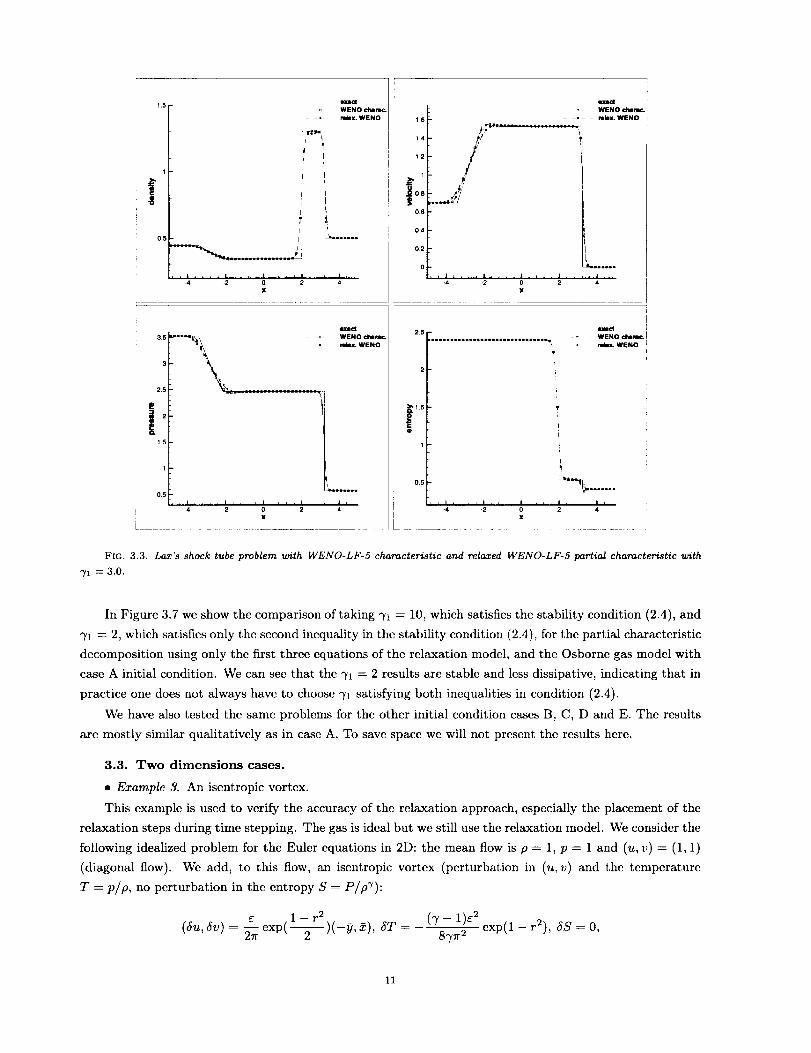
• Example 2. 1D Riemann problems with real gases.

In this example we compute the solutions to the Riemann shock tube problem, for the two molecular

vibrating gas (3.3)-(3.5) and the Osborne model (3.6)-(3.7), with the following initial conditions in Table

3.2.

For this examplc, a uniform grid of 200 points are used and every 4 points are drawn in the figures.

(a)

':i o =,-o

0,8 "

0.7 -

p.i

IM

11

1

09

08

0,7

,,_ 0.8

,_ 0.5

0.4_

0.3

0.2

0,1

0

" /

pmmal _30.0

2

x

11 _-

*It

0.8

0.7

0.6

f

O , I ......... , I ,-4 -2 0 2 4

FIG. 3.2. Sod's shock tube problem with WENO-LF-5. Comparisons of partial and full characteristic decompositions ]or

the relaxation model with _1 -_ 3 (top lcf2); "Y1= 3 and "_z = 30 for the relaxation model with partial characteristic decomposition

(top right); and the relaxation model w_th partial charactemstic decomposition with "Yz = 3 versus the component-wise WENO

applied to the original perfect gas Euler equations.

Also, the "exact solution" in the figures are obtained with the )cst scheme using 2000 points.

We first give a CPU time comparison between the full chara, :teristic decomposition for the original model

and the partial characteristic decomposition using only the first three equations of the relaxation model, for

the two molecular vibrating gas model, in Table 3.3. Wc can see that the partial characteristic decomposition

for the relaxed model is usually more than twice less costly than the full characteristic version for the original

system. Although the relaxed model has one more equation, it does not require the computation of the

complicated derivatives of the EOS.

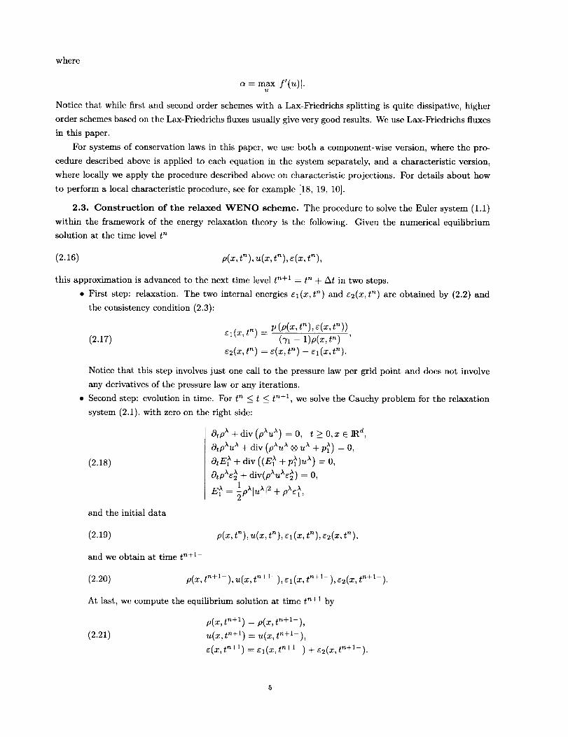
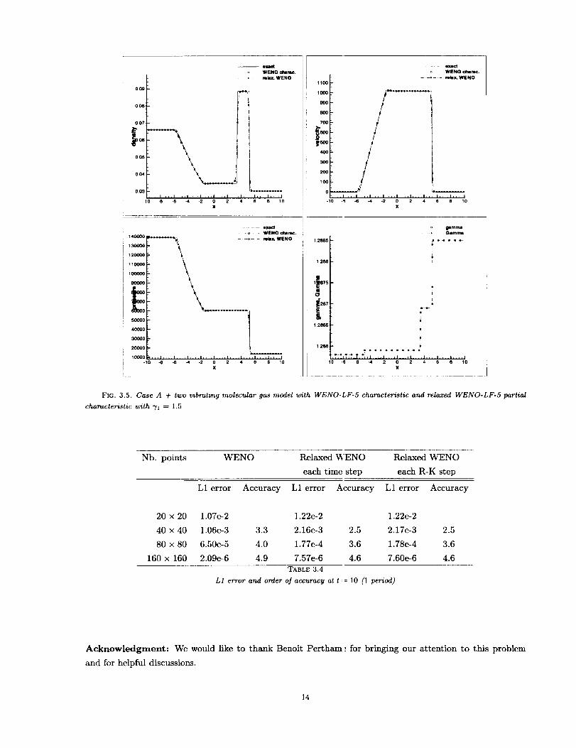
In Figure 3.5 we show the comparison of the full characterk, tic decomposition for the original model and

the partial characteristic decomposition using only the first three equations of the relaxation model, for the

two molecular vibrating gas model, with case A initial condition. The results are almost identical, indicating

that the relaxation model with a partial characteristic decomp(.sition works well with a much reduced cost.

In Figure 3.6 we show the comparison of the component W:_NO scheme on the original system, and the

partially characteristic WENO scheme on the relaxed system with "Yl = 2.0, for the Osborne gas model with

case A initial condition. We can see that the result of the related model is much better, especially for the

density. This indicates that the relaxation model is a good one for the computation of real gases.

10

15

1

|

mmct

WENO charm,

• relax. WENO

• , i .... I .... i , , , i .... I ,-2 0 2 4

x

, .)lmx. WENO

x

2s "f

1.5

1

0.5. i .... i , , , i .... i .... i , ,

-4 -2 0 2 4x

1.6

1.4

1.2

1

0.6

04

0.2

0

2.5

2

1.5

e

1

e]mct

WENO chin mr..

• mime. WENO

F'-----i

t!__4

, i .... i .... ! .... i . .-4 -2 0 2

x

exad

-_ WENO chrome.!

, m;mx. WENO

05l .4 -2 0 2 4

FIc. 3.3. Lax's shock tube problem with WENO-LF-5 characteristic and relaxed WENO-LF-5 partial characteristic with

",/]. = 3.0.

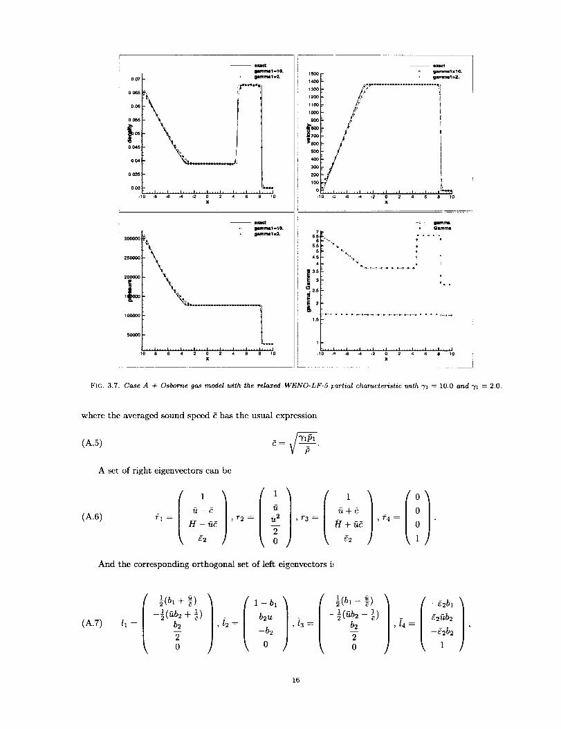
In Figure 3.7 we show the comparison of taking 71 = 10, which satisfies the stability condition (2.4), and

7z = 2, which satisfies only the second inequality in the stability condition (2.4), for the partial characteristic

decomposition using only the first three equations of the relaxation model, and the Osborne gas model with

case A initial condition. We can see that the 71 = 2 results are stable and less dissipative, indicating that in

practice one does not always have to choose 71 satisfying both inequalities in condition (2.4).

We have also tested the same problems for the other initial condition cases B, C, D and E. The results

are mostly similar qualitatively as in case A. To save space we will not present the results here.

3.3. Two dimensions cases.

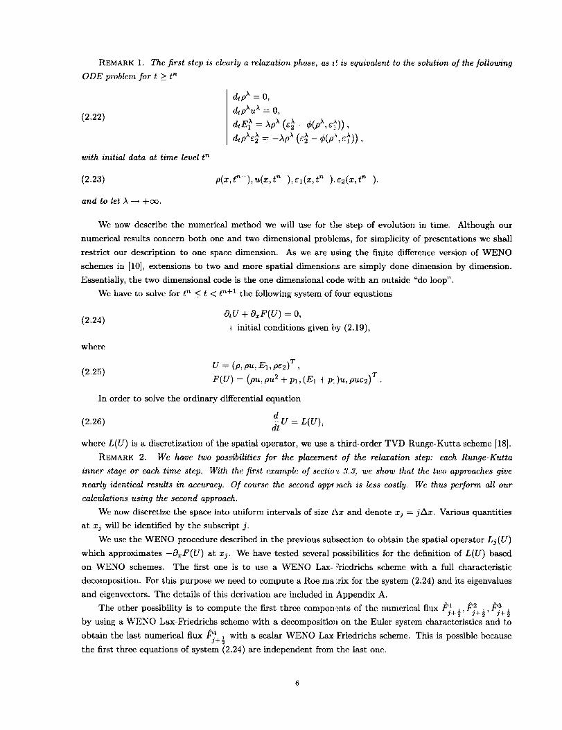
• Example 3. An isentropic vortex.

This example is used to verify the accuracy of the relaxation approach, especially the placement of the

relaxation steps during time stepping. The gas is ideal but we still use the relaxation model. We consider the

following idealized problem for the Euler equations in 2D: the mean flow is p = 1, p -- 1 and (u, v) = (1, 1)

(diagonal flow). We add, to this flow, an isentropic vortex (perturbation in (u, v) and the temperature

T = p/p, no perturbation in the entropy S = PIp'Y):

c 1 - r 2 (7 - 1) C2 exp(1 - r2), 5S = O,(Su,_v) = _-exp(_)(-y, 2), _T-8_r 2L7F _

11

15

I05

md

lilllil¢i'iilm¢..

, lull ctillm_

LIJ

, _ I .... i .... i .... i .... i , ,

-4 -2 0 2 4X

(Is)

1.5

1

I0.5

Ji

, i .... i .... i .... i

-,1. -2 0 2II

(e)

15

1

|05

, , i < , , i .... i , , , i ,

-4 -2 0 2

x

WENO m)ml_. !

- • mix. WENO J

I! =' i'j1

i I i i4

exl(:t

gamrnlll=3.0

• lamm|l=30.O

!! b;I i!:

P _

'L.... i , ,

4

FIC. 3.4. Lax's shock tube problem with WENO-LF-5. Comparisons of partial and lull characteristic decompositions for

the relaxation model with _1 = 3 (top le_t); _1 = 3 and ?z = 30 ]or the relaxation model with partial characteristic decomposition

(top right); and the relaxation model with partial characteristic decornposztion with ?1 = 3 versus the component-wise WENO

applied $o the original perfect gas Euler equations.

where (_,/)) = (x - 5, y - 5), r 2 = _2 +/)2, and the vortex stre]igth E = 5. See [21].

The computational domain is taken as [0, 10, ] × [0, 10], ex ;ended periodically in both directions. This

allows us to perform long time simulation without having to de al with a large domain.

It is clear that the exact solution of the Euler equation wit h the above initial and boundary conditions

is just the passive convection of the vortex with the mean velocity.

In Table 3.4 we show the accuracy result at t -- 10 (one time period). We can see that WENO for the

relaxed model with Yl = 3 gives a somewhat larger error than _-ENO applied directly to the original system,

but the order of accuracy is correct. Moreover, to place the rela::ation step for each Runge-Kutta inner stage

or just for each time step seems to give almost identical results. We have thus used the less costly version of

putting the relaxation step for every time step in all the numez ical examples in this paper.

• Example 4. Double Mach reflection.

The computational domain is chosen to be [0, 4] × [0, 1], altl ough only part of it ([0, 3] × [[0, 1]) is shown.

The reflecting wall lies at the bottom of the computational dormin starting from x = 1/6. Initially a right-

moving Mach 10 shock is positioned at (x,y) = (1/6,0) and :hakes a 60 ° angle with the x-axis. For the

bottom boundary, the exact post-shock condition is imposed for the part from x = 0 to x = 1/6 and a

12

Case State Density Velocity Specific intcrnal

energy

A Left 0.066 0.0 7.22e6

Right 0.030 0.0 1.44e6

B Left 1.40 0.0 2.22e6

Right 0.14 0.0 2.24e6

C Left 1.2900 0.0 1.95e6

Right 0.0129 0.0 2.75e6

D Lcft 1.00 0.0 2.00e6

Right 0.01 0.0 2.50e5

E Left 0.01 2200.0 1.44e5

Right 0.14 0.0 4.00e5

TABLE 3.2

Initial conditions for the test cases for real gases

Case WENO Relaxed WENO with

with characteristic partial characteristic

A 12.68 5.21

B 4.8 2.63

C 12.53 4.87

D 15.0 5.35

E 15.0 7.84

TABLE 3.3

CPU time (in seconds) depending on full or partial characteristic decomposition with a two vibrating molecular gas.

reflective boundary condition is used for the rest. At the top boundary of our computational domain, the

flow values are set to describe the exact motion of the Mach 10 shock. See [23] for a detailed description of

this problem.

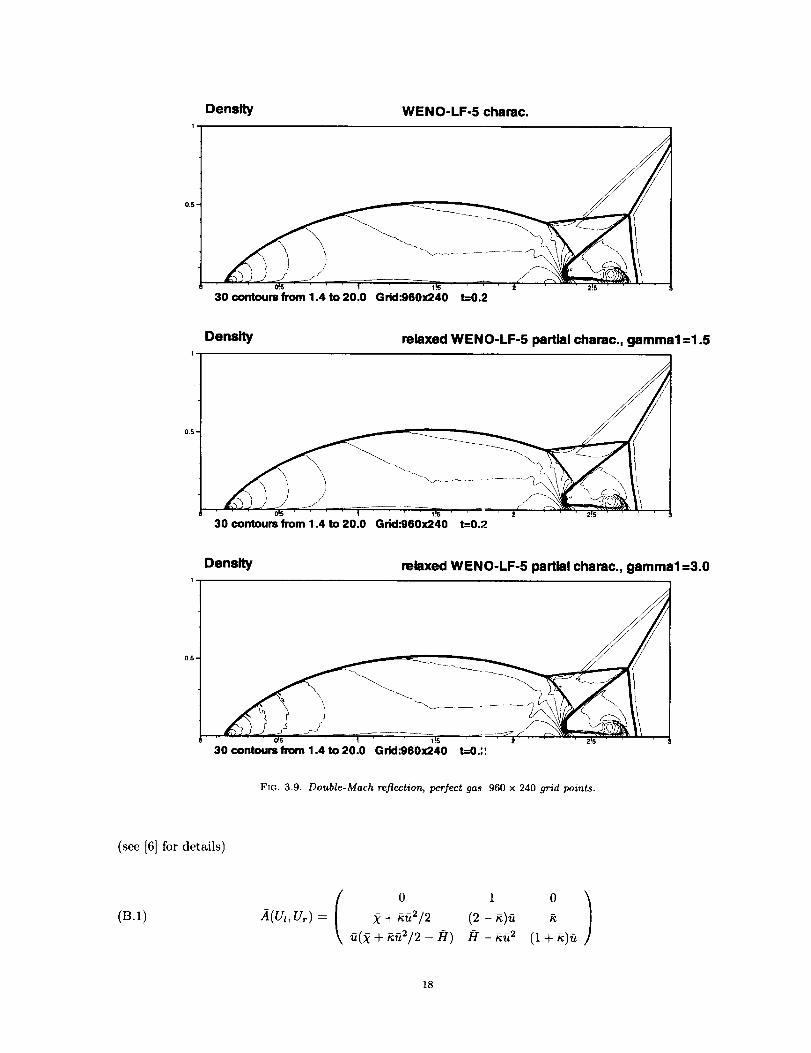
First we present the results for a perfect gas. We compare the results using WENO directly on the

original system [10], and using it on the relaxed model with _1 -- 1.5 and "_1 = 3.0, in Figure 3.8 for a mesh

of 480 x 120 points and Figure 3.9 for a mesh of 960 x 240 points. We can see that the relaxed model results

are quite satisfactory, although a bigger "Y1 results in some small oscillations.

Next, we show the results of the same problem with the two vibrating molecular gas. The purpose here

is to show that thc relaxation model based algorithm does work, rather than on the details of the flow with

more physical models. The results with both a 480 × 120 grid and a 960 x 240 grid are shown in Figure 3.10.

Comparing with the results in [3], we can see that the main features such as the main shock being closer to

the bottom boundary, and the shock below the triple point being bent, are also observed here.

4. Concluding Remarks. Wc have applied the fifth order WENO schemes to a relaxation model

to compute the Euler equations of real gases. The algorithm does not depend on the specific form of the

equation of states and does not need to compute the derivatives of the pressure law. One and two dimensional

examples are shown to illustrate the accuracy and robustness of the algorithm.

13

-- e]md

WENO ¢hamc,

mklx. WENO

0.09 _"%'

0.09'

005 I

003,,,i .... i .... i ,,i .... | .... l, ,,I .... i .... i .... i

-10 -0 _ -4 -2 0 2 4 6 8 10

X

[

140000

" 130(]00

120000

110000

100000

9o0oo

50000

30OOO

20O00

10O0O-10

exit

o WENO ¢hamc.

.... _ WENO

I

,,,i .... i .... l, ,L[ .... i .... i .... i .... i .... i .... i

-8 -6 -4 -2 0 2 4 6 0 10

x

1100

exact

WENO ¢hnraK:.

...... relax. WENO

1000

9oo

BOO

7OO

P

IO0

o _,,_1 .... i .... i L ' ' I .... I .... I .... I .... _ .... _ .... /

o-10 -_ -6 -4 -2 0 2 4 6 0 1X

91ram• Gamma

1.28851- .p - _ - - *v

I

1.280 I- i

I

'I_875

II Lo !

if,o,F ....:E [ ,

1 2885 I-" I

1.286t*gl*_OI04*

-10 "_ -8 ",4 -2 0 2 4 6 8 10

X

FIG. 3.5. Case A + two vibrating molecular gas model with WENO-LF-5 characteristic and relaxed WENO-LF-5 partial

characteristic with _[1 = 1.5

Nb. points WENO Relaxed V_'ENO Relaxed WENO

each time step each R-K step

L1 error Accuracy L1 error Accuracy L1 error Accuracy

20 × 20 1.07c-2 1.22e-2 1.22e-2

40 × 40 1.06c-3 3.3 2.16e-3 2.5 2.17c-3 2.5

80 × 80 6.50e-5 4.0 1.77e-4 3.6 1.78e-4 3.6

160 × 160 2.09e-6 4.9 7.57e-6 4.6 7.60e-6 4.6

TABLE 3.4

L1 error and order of accuracy at t := 10 (1 period)

Acknowledgment: We would like to thank Benoit Pertham,_ for bringing our attention to this problem

and for helpful discussions.

14

0.07

0.065

0.06

0.055

t_05

0.045

0.03

-10

-- ezl_

WENO compo,

, mbuL WENO

,,:1 .... ! .... i .... i .... a .... I .... i .... ! .... lll,,I-8 -6 _I -2 0 2 4 6 8 10

1500

14001

13O0 I

1200 I

11001

10001

9001

lboo]

5001

4001

300 I

200 I

1001

-_ WENO ¢ompo,

• mlmL WENO

...... :-: .... :-:-:-: ....... :

/:,,,,i .... i .... i .... | .... i .... z .... ! .... i .... i,

-I0 "8 -6 -4 -2 0 2 4 6 8 10

X

-- exact

- WENO c_mpo.- -.- relax. WENO

300000

25OOO0

T °

100_ _50OOO

,,,i .... i .... i .... i .... i ,,i .... i .... i .... i .... /0-10 -8 -6 -4 -2 0 2 4 6 8 1

x

FIG. 3.6. Case A + Osborne gas model with component-unse WENO-LF-5 Jor the original system and relaxed WENO-LF-5

partial characteristic with _/] = 2.0.

Appendix A. Roe matrix for the relaxation system.

Let us consider two states Ut and Ur, then the Roe matrix for the relaxation system (2.24) is the following

(A.1) A(UI, U,-) =

0 1 0 0 /

fi2(9"1-- _- --('T1 -- 3)fi'_ (9'1 -- 1) 0

3) ,_

U(--/_I -Jr- (_1 -- 1)_-) /_1 -- (9"1 -- 1)U 2 9"1 _ 0

--g2u g2 0 0,

where the averaged state fi, fi,/-I1 are defined by

(A.2)

with

H1 = alHz, + a_.Hl_, g2 ---- O/l_'l, -[- O_rel.,

(A.3)H1 = (el + Pl)/P,

4-f+4_' a,- = 1 --oq -- v_- ,,_+,/_;.

The four eigenvalues of .zi are

(A.4) 0"1 -_- U -- C_ a2 : u, a3 ----u -{- C-, a4 : "a,

15

0.07

0.065

0.06

0065

0.045

0,114

0035

0,03,,,i .... n .... i .... i .... n .... i .... i .... ! .... i,

-1o `8 -6 -4 -2 o 2 4 6

x

T7lO

-- ixact

-o gammal=lO.

-,- • Bmmmalm2.

250000 _

200111111

1 _000 .

-10 -8 -6 _, -2 0 2 4 6 8 10X

-- exlDct

1500 _- g11_I)11 =10.gamma1 =2.

1400 F-

'=r '71'°°I: #1100 F

O_,,.L .... i .... ! ,,i ,,! .... | .... ! .... i .... n_

-10 -_ _ 4 -2 0 2 4 6 8 10

X

gamma• Gllmma

6.5 _ _ _

5. • , I

51 "-4.51 _" , I"_ ? Y

41 " e I

13-slE _f ,.,

.2.5

i'1.51

lb

,,L| .... I .... I .... I ,,,I .... I .... I .... I .... I,,ll |"10 "8 -8 "4 --2 0 2 4 6 8 10

x iL................ 1

FIc. 3.7. Case A + Osborne gas model with the relaxed WENO-LF-5 partial characteristic w/th "/] ---- 10.0 and "Yl = 2.0.

where the averaged sound speed _ has the usual expression

(A.5)

A set of right eigenvectors can be

(A.6) /1/l i/ //°/---- r2 ---- _2 , r3 ---- ----_ /_-u_ ' -_- h_+_e ,_4 o "

_2 0 g2 1J

And the corresponding orthogonal set of left eigenvectors i,'

(A.7)

(bl + _) 1 - bl

l/fib -- 1_--_l 2 T c/ b2_2

' -b2

0 0

_(bl - c) -_2bl1 - 1

- _(ub2 - c) [4 ---- g2ub2

b2 , ,

k 0 1

16

0.5

Density WENO-LF-5 charac.I

0,5

Density relaxed WENO-LF-5 partial charac., gamma1 =1.5

0.5'

Density relaxed WENO-LF-5 partial charac., gamma1=3.0

where

(A.s)

FIG. 3.8. Double-Mach reflection, perfect gas, 480 x 120 grid points.

bl- (_l-1)u 2 b2- (_/1-1)2_2 ' C_2

Appendix B. Roe matrix for a two molecular vibrating gas.

Let us considcr two states Ul and Ur, then the Roe matrix for an Euler system of real gas is the following

17

0.5

Density WENO-LF-5 chamc.1

30 contours from 1.4 to 20.0 Grid._60x240 t=0.2

05

Density reiaxed WENO-LF-5 partial charac., gamma1 =1.5

30 contours from 1.4 to 20.0 Grid:060x240 t=0.2

DensltyI

relaxed WENO-LF-5 partial charac., gamma1 =3.0

0.5,

.... 4 ...... _ _ 1 _5 I r _ 2 5

30 contours from 1.4 to 20.0 Grid:960x240 t=0.:!

FIc. 3.9. Double-Mach reflection, per]ect gas 960 × 240 grid points.

(see [6] for details)

(B.1)0 1 0 /

A(_]_,ur) = _ + _/2 (2 - _)_

_(2 + _2/2 - H) //- _ (1 + _)_

18

Density Real gas relaxed WENO-LF-5 partial chamc., gamma1 =1.5I

0,5,

1-

0_5-

Density Realgas relaxed WENO-LF-5 partial chamc., gamma1 =1.5

/

30 contour_rom 1.4to3110 Grid:960x_0' t=0.2 ' ' .... 2_ ....

FIG. 3.10. Double-Mach reflection, two vibrating molecular gas.

where _,/t are the Roe-average values of the velocity and the total specific enthalpy (H = E + 1/2u 2 + p/p)

(B.2) u = v_Ut + v/_u_v_ + v_; '

(B.3) /t = x/_Hl + x/_Hrv_ + v'_ '

and _ and _ are two parameters which must satisfy

(B.4) Ap = kApe + ](Ap

with Ap = p_ - Pl, ApE = pre_ -- ptel and Ap = p(p_, er) - P(Pt, et).

(B.5)

(B.6)

The definitions for _ and _ proposed by In [9] for a two molecular vibrating gas are

r(T(e")--T(eO) if e_ # el,Er --e l

k = a (p • (re,e) + p,. (p_,e) _ r2_ m _j = _ ifer =et =e,

Ap

l(p,p(p, _) _ 9p,_(p, e_)+ pap, er) - 9p,_(p, _))= ½r(T(et)- tiT'(el)+ T(er) - e_T'(e_))

if Pr # Pt,

ifpr :Pt :P.

19

The definitions of the eigenvalues and right and left eigenvectors are easy to obtain and arc omitted

here.

REFERENCES

[1] P. COLELLA AND H. M. GLAZ, Et_cient solution algorithms for the Riemann problem for real gases,

J. Comput. Phys., 59 (1985), pp. 264-289.

[2] F. COQUEL AND B. PERTHAME, Relaxation of energy and approximate Riemann solvers for general

pressure laws in fluid dynamics equations, SIAM J. Numer. Anal., to appear.

[3] R.L. DESCHAMBAULT AND I.I. GLASS, An update on non-stationary oblique shock-wave reflections:

Actual isopycnics and numerical experiments, J. Fluid Mech., 131 (1983), pp. 27 57.

[4] P. GLAISTER, An eI_cient numerical method for compressible flows of a real gas using arithmetic

averaging, Comput. Math. Appl., 28 (1994), pp. 97 113.

[5] --, An analysis of averaging procedures in a Riemann solver for compressible flows of a real gas,

Comput. Math. Appl., 33 (1997), pp. 105 119.

[6] E. GODLEWSKI AND P.-A. RAVlART, Numerical approximation of hyperbolic systems of conservation

laws, Springer, 1996.

[7] B. CROSSMAN AND R. W. WALTERS, Analysis of flux-split algorithms for Euler's equations with real

gases, AIAA J., 27 (1989), pp. 524- 531.

[8] A. HARTEN, B. ENGQUIST, S. OSHER AND S. CHAKRAVARTHY, Uniformly high order essentially non-

oscillatory schemes, III, J. Comput. Phys., 71 (1987), pp. 231 303.

[9] A. IN, Numerical evaluation of an energy relaxation method for inviscid real fluids, EDF research report

HT-13/97/032/A, submitted for publication.

[10] G.-S. JIANG AND C.-W. SHU, Efficient implementation of weighed ENO schemes, J. Comput. Phys.,

126 (1996), pp. 202 228.

[11] B. LARROUTUROU, How to preserve the mass fractions l_sitivity when computing compressible multi-

component flows, J. Comput. Phys., 95 (1991), pp. 59 84.

[12] P. D. LAX, Weak solutions of non-linear hyperbolic equations and their numerical computations, Com-

mmun. Pure Appl. Math., 7 (1954), pp. 159 193.

[13] M. S. LIOU, B. VAN LEER, AND J.-S. SHUEN, Splitting of inviscid fluxes for real gases, J. Comput.

Phys., 87 (1990), pp. 1 24.

[14] X.-D. LIu, S. OSHER, AND W. CHAN, Weighed essentially non-oscillatory schemes, J. Comput. Phys.,

115 (1994), pp. 200 212.

[15] C.-V. LOH AND M. S. LIOU, Lagrangian solution of supersonic real gas flows, J. Comput. Phys., 104

(1993), pp. 150 161.

[16] J.-L. MONTAGNE, H. C. YEE, AND M. VINOKUR, Comparative study of high-resolution shock-capturing

schemes for a real gas, AIAA Journal, 27 (1989), pp. 1332-1346.

[17] T. D. RINEY, Numerical evaluation of hypervelocity impcct phenomena, in High-velocity impact phe-

nomena, R. Kinslow, ed., Academic Press, 1970, ch. V pp. 158 212.

[18] C.-W. SHU AND S. OSHER, Efficient implementation 6f essentially non-oscillatory shock-capturing

schemes, J. Comput. Phys., 77 (1988), pp. 439 471.

[19] C.-W. SHU AND S. OSHER, El_icient implementation cf essentially non-oscillatory shock-capturing

schemes, II, J. Comput. Phys., 83 (1989), pp. 32 78.

2o

REPORT DOCUMENTATION PAGEFormApprovedOMB No. 0704-0188

Pubtlcreportingburdenfor thiscollectionofinformationisestimatedtoaverage1hourperresponse,includingthetimeforreviewinginstructions,searchingexistingdatasources,gatheringandmaintainingthedataneeded,andcompletingandreviewingthecollectionofinformationSendcommentsregardingthisburdenestimateor anyotheraspectofthiscollectionofinformation,includingsuggestionsfor reducingthisburden,toWashingtonHeadquartersServices.Directoratefor InformationOperationsandReports,1215JeffersonDavisHighway,Suite1204.Arlington,VA222024302,andto the Officeof ManagementandBudget,PaperworkReductionProject(0704-0188),Washlng-ton,DC20503.

1. AGENCY USE ONLY(Leaveblank) 2. REPORT DATE 3. REPORT TYPE AND DATES COVEREDSeptember 1998 Contractor Report

4. TITLE AND SUBTITLE 5. FUNDING NUMBERS

Real gas computation using an energy relaxation method and high-order WENO schemes

6. AUTHOR(S)

Philippe Montarnal

Chi-Wang Shu

7. PERFORMING ORGANIZATION NAME(S) AND ADDRESS(ES)

Institute for Computer Applications in Science and Engineering

Mail Stop 403, NASA Langley Research Center

Hampton, VA 23681-2199

9. SPONSORING/MONITORING AGENCY NAME(S) AND ADDRESS(ES)

National Aeronautics and Space Administration

Langley Research Center

Hampton, VA 23681-2199

C NAS1-97046

WU 505-90-52-01

8. PERFORMING ORGANIZATIONREPORT NUMBER

ICASE Report No. 98-42

10, SPONSORING/MONITORINGAGENCY REPORT NUMBER

NASA/CR-1998-208712

ICASE Report No. 98-42

11. SUPPLEMENTARY NOTES

Langley Technical Monitor: Dennis M. Bushnell

Final ReportSubmitted to Journal of Computational Physics

12a. DISTRIBUTION/AVAILABILITY STATEMENT

Unclassified Unlimited

Subject Category 64

Distribution: Nonstandard

Availability: NASA-CASI (301)621-0390

12b. DISTRIBUTION CODE

13. ABSTRACT (Maximum200 words)In this paper, we use a recently developed energy relaxation theory by Coquel and Perthame and high order weighted

essentially non-oscillatory (WENO) schemes to simulate the Euler equations of real gas. The main idea is an energy

decomposition into two parts: one part is associated with a simpler pressure law and the other part (the nonlineardeviation) is convected with the flow. A relaxation process is performed for each time step to ensure that the originalpressure law is satisfied. The necessary characteristic decomposition for the high order WENO schemes is performedon the characteristic fields based on the first part. The algorithm only calls for the original pressure law once pergrid point per time step, without the need to compute its derivatives or any Riemann solvers. Both one and twodimensional numerical examples are shown to illustrate the effectiveness of this approach.

14. SUBJECT TERMS

Euler equations; real gas; weighted essentially non-oscillatory schemes

17. SECURITY CLASSIFICATION 18. SECURITY CLASSIFICATIOI_ 19. SECURITY CLASSIFICATIONOF REPORT OF THIS PAGE OF ABSTRACTUnclassified Unclassified

_/SN 7540-01-280-5500

15. NUMBER OF PAGES

26

16. PRICE CODEA03

20. LIMITATIONOF ABSTRACT

'Standard Form298(Rev. 2-89)PrescribedbyANSIStd Z39-18298-102

[20] C.-W. SHU, T.A. ZANG, a. ERLEBACHER, D. WHITAKER, ,_ND S. OSHER, High order ENO schemes

applied to two- and three- dimensional compressible flow, _ppl. Numer. Math., 9 (1992), pp. 45 71.

[21] C.-W. SHU, Essentially non-oscillatory and weighted essentia;ly non-oscillatory schemes for hyperbolic

conservation laws, in Advanced Numerical Approximation o] Nonlinear Hyperbolic Equations, A.

Quarteroni, Editor, Lecture Notes in Mathematics, CIME subseries, Springer-Verlag, to appear.

[22] G. SOD, A survey of several finite difference methods for systems o] non-linear hyperbolic conservation

laws, J. Comput. Phys., 27 (1978).

[23] P. WOODWARD AND P. COLELLA, The numerical simulation of two-dimensional fluid flow with strong

shocks, J. Comput. Phys., 54 (1984), pp. 125-160.

21