1

Real Options in Offshore Oil Field Development Projects

Morten W. LundNatural Gas Marketing & Supply, Statoil

N-4035 Stavanger, Norway

e-mail: mowlu@statoil.com

Abstract

The average size of discovered petroleum reserves on the Norwegian continental shelf has declined steadily over

the last years. As a consequence, the fields have become economically more marginal, and new and flexible

development strategies are required. This paper describes a stochastic dynamic programming model for project

evaluation under uncertainty, where emphasis is put on flexibility and its value. Both market risk and reservoir

uncertainty are handled by the model, as well as different flexibility types. The complexity of the problem is a

challenge and calls for simple descriptions of the main variables in order to obtain a manageable model size.

Results from a case study reveal significant value of flexibility, and clearly illustrate the shortcoming of today’s

common evaluation methods. Particularly capacity flexibility should not be neglected in future development

projects where uncertainty surrounding the reservoir properties is substantial.

1 Introduction

Since the first discovery of oil on the Norwegian continental shelf back in 1968, the Norwegian

offshore activity has evolved rapidly. In the early years only a handful of companies took interest in

the exploration for and production of oil and gas, and the effect on the mainland activity was minor.

But, as the discovery of vast resources took place, the offshore industry gave nourishment to both

increased employment and sub supplies. Today a total of 17 operators and 10 other licensees are

operating on the shelf, and the oil and gas activity provides approximately 15% of the gross national

product of Norway. In 1997 the production of oil reached 187 million Sm3 oe1, making Norway the

7th largest oil producer in the world. The high rate of activity has made the oil and gas industry a very

important element of the Norwegian economy. Consequently it has lead to a substantial effort directed

towards the search for efficient and cost effective development strategies.

The focus on improved development strategies has strengthened over the last 10-15 years, and can

partially be traced back to the decrease in field size that has been experienced. While the size (5 year

moving average) of discovered reserves in the beginning of the 80’s was between 80 and 100 million

Sm3 oe, the corresponding figures since 1990 has been below 20 million Sm3 oe. The reduced size has

made new fields become economically more marginal, and has put emphasis on the need for so-called

flexible development strategies.

1 oe - oil equivalent.

2

A number of contributions have addressed the subject of investment under uncertainty in the oil

industry. Especially the development of contingent claims analysis and its applications to real

investments have provided increased insight into this topic. However, these contributions typically

assess one type of flexibility, ignoring the interrelations between different flexibility types (Ekern

(1988), McDonald and Siegel (1986), Olsen and Stensland (1988), Pickles and Smith (1993),

Stensland and Tjøstheim (1991), Triantis and Hodder (1990)). Most of the published examples also

greatly simplify the project description, by including only one stochastic variable. As a consequence,

it is hard to discern the benefit of flexibility in a realistic oil field development project from

contributions reported in the literature.

Worth mentioning is also that the presence of technical (e.g., reservoir properties) as well as market

(e.g., oil price) uncertainty challenges the foundation for use of option pricing theory. However, by

assuming the existence of certain market and preference conditions Smith and McCardle (1998) show

that technical (and market) uncertainty can be included in a valuation procedure integrating option

pricing and decision analysis approaches. Compared to the contributions relying solely on contingent

claims analysis, they develop an extended continuous time model for valuation of an oil property in

which the decision maker has the flexibility to terminate the project or accelerate production by

drilling additional wells. Two stochastic variables are captured, the well production rate and the oil

price.

Finding the value of flexibility in an offshore oil field development project by use of stochastic

dynamic programming represents an alternative approach to project assessment under uncertainty.

Few examples though of models covering the complete project, from inception to abandonment, exist.

Bjørstad et al (1989) analyse the value of an oil prospect given that four decisions (develop, explore,

wait and stop) can be made at each stage. The oil price and the recoverable volume are assumed

stochastic, while the cash flow profile is based on expected values. A similar model is given in

Tennfjord (1990). Smith and McCardle (1996) present a model where the decisions to wait, abandon,

invest in tankers and tie in nearby fields provide the operator with flexibility. In addition to price and

cost uncertainty, the reservoir production is uncertain. A common trait of these models is that

managerial flexibility during the production phase is neglected. For most projects this flexibility is an

important feature which allows the operator to make corrective adjustments and changes to the

depletion strategy as new knowledge is acquired. As an example, consider a field where the well rate

suddenly drops. Being able to adjust the depletion rate, e.g., by drilling new production wells, might

then be of significant value. This value should be included in project assessments.

The model described in this paper seeks to capture the main types of flexibility present in oil field

development projects. These are initiation, termination, start/stop, information and capacity

flexibility. Of particular interest is the capacity flexibility, i.e., the option to change the scale of the

project. This may be achieved by changing the production capacity of the production unit, and/or by

changing the production capacity of the reservoir. Compared to related models, as given by Bjørstad

et al (1989) and Smith and McCardle (1996), the presented framework represents a significantly

extended approach. Both the degree of decision making freedom and the number of stochastic

variables are increased, implying a much more computationally demanding model. The associated

3

value of using the extended model is identified by the results from a case study based on an ongoing

development of an oil reservoir.

The paper is organised as follows. Section 2 of the paper presents the problem, and gives the main

assumptions made in the analysis. In section 3 the model is outlined. The modelling of the stochastic

variables is addressed, and the operator’s flexibility is described. Size and computational performance

are also assessed. The following section, section 4, illustrates the benefit of flexibility in an oil field

development project. Section 5 contains some final remarks and comments to the proposed model.

2 Valuing offshore oil field development projects

The development of an offshore oil field is a task characterised by its versatility and high degree of

uncertainty. The selection of the development strategy is made early in the project’s lifetime, and at

the time the decision is made the information concerning the field is often scarce. For instance is

neither the future production nor sales prices known with certainty. The problem facing the decision

maker is therefore a problem with imperfect information. This makes the decision making process a

challenging one, and the methods applied should offer adequate support for evaluation under

uncertainty. The criticality of good decision making at this stage is further stressed by the fact that the

choice of a development strategy is of great consequence for the profitability of the project.

Several decades may pass between inception and completion of the project, and throughout this time

many disciplines are involved. A model that aims to cover the complete development must therefore

be based on rather crude approximations in order to get a solvable model. The requirement for a

compact representation of the problem is of course not unique to an oil field development project, but

the inherent complexity makes this demand a critical one. To facilitate the modelling the project is

thus depicted by a simple phasing (figure 1). The four phases cover the complete development project

from the time before the PDO (Plan for Development and Operation) is submitted to the government

to the abandonment.

Engineering and construction

Exploration Conceptual study Production

time

Fig. 1 Phases of an oil field development project.

The operator bases the PDO on information about the reservoir properties retrieved by seismic

surveys and exploration well drilling. It is however still possible to obtain further information by

additional well drilling, as captured by the exploration phase. Having completed the appraisal of the

reservoir the conceptual study is carried out. The choice of concept involves, in addition to the

selection of a production unit, a choice of flexibility. As any possibility to alter the configuration of

4

the production unit is restricted by its free space and carrying capacity, the concept design is essential

to the development strategy. Following the choice of concept is the engineering and construction of

the production unit. This may either be the construction of a new unit, or the modification of an

existing unit. Finally the depletion of the field is captured in the production phase.

The value of flexibility is closely related to the uncertainty. An analysis of flexibility must therefore

be made together with an assessment of the uncertainty surrounding the project. Hence, the selection

of stochastic variables should support the flexibility of interest. Based on previous studies and

discussions with Norwegian operators three variables are considered stochastic in the model; the oil

price, the reservoir volume, and the well rate. These variables are of major importance to the

production profile and the cash flow of the field.

To find the optimal development strategy for the field it is assumed that the operator is risk neutral2.

Considering the size of most oil companies this is a reasonable assumption. The objective is thus to

maximise the expected net present value of the project. The scope of the analysis is a single field, and

the economic assessment is made before tax. It is also assumed that the field is developed by a

moveable production platform (a semi-submersible), even though this is not a requirement for the

model. The moveable platform is merely a choice of convenience.

3 Outline of the model

In the discussion below the phasing given in figure 1 is followed. Emphasis is put on the structure to

provide an intuitive understanding of the model’s layout and properties. For a more thorough

discussion of the model and its features the reader is referred to Lund (1997).

The model is an optimisation model of discrete stages, where sequential decision making is made in a

stochastic environment. It is assumed that the transition probability from the current to the next state

of the process (the field development project) only depends upon the current state. Hence, the model

is a Markov decision process. Since Norwegian regulations specify that the licencee must develop

(and produce) the field within a period of maximum 40 years after the production licence is awarded

(NOE (1997)), the problem is of finite horizon.

2 A risk neutral attitude implies that a person considers the utility of a certain prospect of money to be equal to the expectedutility of an uncertain prospect of equal expected monetary value

5

A period of 40 years is in this context regarded as long, in the sense that an approximation by an

infinite horizon might yield acceptable results. However, the limit of 40 years represents a maximum,

and the operator may face a shorter horizon. For instance can scheduled activities in neighbouring

areas restrict the field development horizon. Thus in order to develop a robust model which can be

applied also for shorter horizons the assumption of a finite horizon is kept.

Each stage in the model is a decision epoch that represents a time lag for the consequence of an action

to materialise. To keep the model at a manageable size, a maximum of 20 stages (and epochs) is

applied. The length of the decision epochs is a parameter in the model, and should be set to a suitable

value for the field development project considered. All costs and incomes are related to the start of the

decision epochs.

3.1 Exploration

Exploration constitutes a substantial share of the investment activity at the Norwegian continental

shelf. The typical cost of an exploration well is today USD 15 million, and in the last decade the

exploration has amounted to 10 to 30 percent of the accrued investment costs. Including exploration

in the model should therefore improve the analysis significantly.

The basis for the reservoir assessment is the operator’s a priori probability distributions of the

(technically recoverable) reservoir volume and the well rate. These distributions are typically obtained

through seismic surveys (the volume) and wildcat wells. However, it is possible for the operator to

obtain more information about the reservoir volume before the development starts (i.e., the operator

has what is here termed information flexibility). In the model this is achieved by drilling of additional

exploration wells.

Drilling of additional exploration wells is restricted to periods before the conceptual choice is made.

The wells are drilled in clusters of predetermined size, where a cluster may comprise one or several

wells. Information received from the well(s) is assumed binary, and either indicates a low volume or a

high volume. (Perfect information about the reservoir volume is only obtained through production.)

The indication of a low volume corresponds to the well(s) not hitting oil, while indication of a high

volume is obtained if the well(s) hits oil. The probability of receiving a given well information is

conditional upon the true reservoir volume, and the information is used to update the operator’s

probability distribution in a standard Bayesian manner (see e.g., Pratt, Raiffa and Schlaifer (1995)).

3.2 Conceptual study

A concept is here defined by the installed production capacity of the platform and the option to

increase this capacity during the production phase. The production capacity of the platform should in

this context be conceived of as a combined measure of the platform’s production, processing and

storing facilities. Hence, the production capacity specifies the total well stream that can be handled by

the platform. In the conceptual study phase the operator thus decides the initial production capacity of

the concept, as well as the possibility of increasing the capacity at later stages (capacity flexibility). A

concept where the production capacity can be increased at subsequent stages, i.e., during the

6

production phase, requires both additional space, e.g., on the platform deck, and extra carrying

capacity. This induces additional costs, which can be considered costs of obtaining flexibility. Where

convenient the production capacity will be referred to as simply the capacity of the platform.

The conceptual study phase also includes the decision of pre-drilling of production wells. This to

make sure that the production of oil can start immediately after the production unit is located at the

field. Without pre-drilled wells the operator might experience a delay due to drilling of production

wells after the production unit has been constructed. (It is not possible to convert exploration wells to

production wells in the model.) It is further assumed that the first production well reveals perfect

information about the well rate for the first production period.

3.3 Engineering and construction

The engineering and construction phase does not contain any decisions, but carries out the decisions

made in the conceptual study phase. Any pre-drilling of production wells decided in the conceptual

study phase is done during this phase.

It is assumed that the time spent on engineering and construction is independent of the selected

concept (cf. Wallace et al (1985a)), and any differences between various concepts are therefore

limited to the construction and operating cost, the installed capacity and the flexibility to increase the

capacity. Construction cost for the production unit (the semi-submersible) is related to the installed

capacity and the possibility to expand the capacity at subsequent stages. The cost is positively related

with both. That is, the higher the installed capacity is, the higher is the construction cost, and the more

capacity flexibility the platform offers, the more costly is the concept.

3.4 Production

During the production phase the flexibility arises from the operator’s option to decide the level of

production, the drilling of production wells and, if possible, any increase in production capacity of the

production unit. Both the drilling of production wells and any increase of the platform’s production

capacity are examples of capacity flexibility.

Reservoirs are by nature three-dimensional, and should be modelled by three-dimensional models.

However, the computational demand of such models (cf. Lia et al (1995)) inevitably hampers their

usefulness in a comprehensive framework. Thence, a much simpler approach is proposed, in which

the maximum production level is described by a zero-dimensional tank model with perfect

communication throughout the reservoir. The complete tank model is described in Appendix A.

Compared to the complex realism of a reservoir a model without spatial variations necessarily

represents a crude approximation. However, the tank model is able to depict a typical production

profile (cf. Lund (1997)), and has been widely applied in analysis of field developments (Aronofsky

and Williams (1963), Frair and Devine (1975), Beale (1983), McFarland et al (1984)). The tank

model used here is described in Wallace et al (1985b), and defines the maximum production from the

field at time t, qmax,t, by (1).

7

{ }q N q q qt t w t p t r tmax, , , ,min � , ,= ⋅ (1)

where Nt: number of producing wells at time t

� ,qw t: production capacity of a well at time t

qp,t: production capacity of the platform at time t

qr,t: maximum reservoir depletion rate at time t (productivity of the reservoir at time t)

The well rate, and thence the production capacity of a well (see appendix A), follows a Markov

process, where transition takes place if the field is producing. The capacity of the wells for the next

production period is revealed at the end of the present production period. Hence, the production

capacity is assumed known when the production decision is taken. Without any production the

production capacity of a well remains the same.

By modelling the reservoir volume and the well rate as stochastic variables the (originally

deterministic (cf. Wallace et al (1985b)) tank model provides a production profile with stochastic

escalation, plateau level and duration, and decline. This is considered adequate to describe the

uncertainty surrounding the reservoir at an early stage of the development. Note that the assumption

of a stochastic well rate is not in accordance with the foundation for the tank model, which requires a

homogenous and well behaved reservoir. The tank model should therefore be considered a convenient

framework for development of a simple relationship between important reservoir parameters and the

production profile, rather than a strict condition.

To curtail the model size the production decision is implemented as a binary choice, where the

platform either produces at maximum level or it does not produce at all. This is similar to enforcing a

so-called “bang-bang” solution (cf. Dixit and Pindyck (1994)).

Production wells can be drilled at all stages in the production phase, and the possible number of wells

is independent of platform concept. As for the exploration wells, the production wells are assumed

drilled in clusters of predetermined size, and in a predetermined sequence. The total number of

clusters that can be drilled at the field is restricted by an upper limit. The production wells have

infinite lifetimes, i.e., each well can produce throughout the entire production period.

It is further assumed that the platform capacity can be increased at all stages. Naturally this requires

that the platform concept is designed for optional capacity, and that available space has not been

utilised by previous installations of additional capacity. The increase is only limited by the available

space. Hence, it is possible to use all expansion area at one stage. Capacity expansions are made in

steps of predetermined size. The cost of increasing the capacity is dependent upon the magnitude of

the expansion and (generally) the concept.

During the production phase, the platform incurs fixed operating costs. These are dependent on the

installed capacity and the platform concept, but independent of the production level. In addition there

is a variable cost associated with the production of oil. This cost is given per produced barrel.

8

3.5 Initiation, start/stop and termination

The flexibility described so far is confined to the respective phases. In addition, two decisions that

provide flexibility are available in all phases. First, the operator is allowed to abandon the project at

all stages (termination flexibility). Abandonment implies a cost, which is dependent upon the phase

the project has reached and the number of production wells that must be plugged.

Second, the operator may always choose to just wait (i.e., temporarily stop the development) and not

pick a certain action (initiation flexibility and start/stop flexibility). This can be favourable if the oil

price fluctuates heavily, since by waiting the operator might get a higher price. There is no direct cost

associated with the decision to wait, but if the platform has been constructed the fixed operating cost

accrues.

Based on the preceding discussion of the options available to the operator as the project develops, the

decision space can now be summarised by figure 2. As pointed out the decision making freedom of

the operator depends on the phase of the project, and except for the start/stop flexibility and the

termination flexibility the other flexibility types are phase dependent.

Engineering and construction

Exploration Conceptual study Production

· produce oil · expand platform capacity · drill production wells · start/stop · terminate

· start/stop · terminate

· select concept · pre-drill production wells · start/stop · terminate

· drill exploration wells · start/stop · terminate

· initiate

Fig. 2 Decision space related to phases in the oil field development project.

3.6 Model size and performance

The size of the model, measured by its state space, the number of alternative decisions and the number

of stages, depends on the field development project being addressed as well as the choice of stochastic

process for the oil price. To indicate the performance of the model figure 3 shows solution times for

runs made on two different computers. The reported figures refer to a model with a maximum state

space (last stage) of 1.4 million and a decision space of 38.

As seen from the figure the solution time for the Sun Ultra 2 is less than half the solution time for the

Pentium PC. The gain of going from a PC to a Unix platform (Sun Ultra 2) is mainly related to the

9

faster processor of the latter, which reduces the solution time by approximately 49%. The additional

reduction of 8% is due to a more efficient memory utilisation and less input/output activity.

0

5

10

15

20

25

Pentium,166 MHz

Sun Ultra 2,model 1200

Sol

utio

n tim

e [m

inut

es]

Fig. 3 Solution times for different computers. Maximum state space of 1 404 000.

The reported solution times are considered acceptable for practical decision making situations, and

should not represent a major obstacle for a successful implementation in an oil company. And,

compared to commercially available decision analysis software (DPL™), the efficiency of the

recursive solution procedure is evident. For a much smaller problem described by a decision tree with

approximately 52 500 endpoints Smith and McCardle (1996) report solution times of about 90

minutes. Using this software to solve the model outlined in this paper would yield prohibitive solution

times.

4 The value of flexibility in a small oil field development project

To illustrate the qualities of the developed framework the model has been implemented for a small oil

field about to be developed on the Norwegian continental shelf. The project considered is inspired by

the ongoing development of the Midgard oil reservoir, which is a part of the Åsgard3 field. Project

data are, however, somewhat modified in order not to reveal any restricted information, and the

project described in the following should not be conceived of as the Midgard development. The case

is therefore artificial, but the salient features resemble those of the Midgard oil reservoir.

The addressed oil field consists of a single reservoir which is located at Haltenbanken in the

Norwegian Sea. It will be produced by a semi-submersible, and produced oil is loaded from the

10

platform via a loading buoy onto a crude oil tanker. Offshore loading and unloading at the terminal is

made in a shuttle traffic manner.

Due to scheduled activities in the neighbouring area the field must be developed and depleted within a

maximum time period of 10 years. A total of 20 decision epochs, each of length 0.5 year, is thus used.

Three stochastic variables are considered in the model; the oil price, the well rate and the reservoir

volume. For the considered project these variables and the applied rate of return are specified as

follows:

Oil price. The oil price, P, is modelled as a geometric Brownian motion (2). It has an assumed drift

rate, α, of zero and a volatility, σ, of 0.204. The present price is 18 USD/barrel.

dP

Pdt dz= +α σ (2)

where P : oil price

α: drift rate

t: time

σ: volatility

dz: increment of a Wiener process. E[dz] = 0, Var[dz] = dt

The approximation of the geometric Brownian motion used in the model is a binomial model first

proposed by Cox, Ross and Rubinstein (1979). It has later been widely used to find approximate

solutions to continuous time problems (see e.g., Hull (1993) and Pickles and Smith (1993)). Let P be

the initial oil price. In the binomial model the oil price can then either move up to uP or go down to

dP during the time interval ∆t (fig. 4). The probability of a movement up or down is p and 1 - p,

respectively.

3 The Åsgard field was discovered in the period 1981 to 1985. It consists of three deposits; Midgard, Smørbukk andSmørbukk Sør. The operator of the field is Statoil.4 The volatility reported in the literature is typically in the range of 0.15 and 0.25, depending on the time series used forestimation (Paddock et al (1988), Pindyck (1988), Bjerksund and Ekern (1990)). As a basis, the mean value, 0.20, is usedhere.

11

∆t

P

uP

dP

p

1-p

Fig. 4 Binomial price process.

The parameters of the approximation is determined by the drift rate, α, and the volatility, σ, of the

geometric Brownian motion as follows

u e du

e pe d

u dt t

t

= = = =−

−−σ σ

α∆ ∆

∆

, ,1

(3)

The Brownian motion lends itself to evaluation methods based on options pricing theory. However,

the existence of spanning assets5 (cf. Dixit and Pindyck (1994), p. 117) is a prerequisite for the

evaluation procedure in its original form. The introduction of uncertainty surrounding the reservoir

makes this an unattainable assumption and removes the theoretical foundation for the approach.

Nevertheless, as previously mentioned it is possible to extend the option pricing theory to handle both

hedgeable risk (market risk) and unhedgeable risk (private risk) given that certain market and

preference assumptions are present (Smith and Nau (1995), Smith and McCardle (1998)). Though the

extended approach utilises market information to value market risk, the analysis still requires the use

of subjective preferences and beliefs. The advantage offered by this extended approach compared to a

decision theoretic approach is thus moderate, and taking into account the preference restrictions the

net gain is dubious. Consequently a traditional decision theoretic approach is selected for the model at

hand.

Well rate. Two well production capacities can be realised. One being a low capacity of 0.4 million

Sm3 per year, the other a high capacity of 1.2 million Sm3 per year. The ratio of well production

capacity to maximum well potential, γ, is 0.75 (see appendix A), and the well rates corresponding to

the capacities are then 0.53 and 1.60 [million Sm3/year], respectively.

The operator has a uniform a priori probability distribution of the well rate, i.e., before any production

wells are drilled. The initial well rate uncertainty may seem high, but is reasonable provided that no

test production has taken place. During production the well rate fluctuates between the two states, but

5 This is also known as the “complete markets” assumption, and ensures that an investor is able to perfectly hedge everyproject risk by trading existing securities.

12

the stability is high (table 1). The possible change in rate from one production period to the next

reflects both variations in physical reservoir conditions that may occur (flow barriers, water-coning,

etc.), as well as the operator’s possibility of successfully counteracting such undesirable events. (The

transition of going from well rate i to well rate j is possible once a period.)

Tab. 1 Transition probabilities, pij, of going from

well rate i to well rate j.

Low rate High rate

Low rate 0.9 0.1

High rate 0.1 0.9

Reservoir volume. The reservoir volume has an expected value of 6 million Sm3, with probability

distribution as shown in table 2. The distribution is the operator’s a priori distribution, that is before

any exploration is carried out.

Tab. 2 A priori probability distribution of reservoir volume.

Volume [million Sm3] 2 6 12

Probability 0.3 0.5 0.2

Rate of return. The annual rate of return is commonly recognised as one of the most important factors

for the net present value of a project. Nevertheless, in most operations research contributions the

discount factor is introduced into the problem with little or no discussion regarding its model

implications. A typical example is found in Ross (1983), who states that "The use of a discount factor

is economically motivated by the fact that a reward to be earned in the future is less valuable than one

earned today.". A similar assessment is given in Dixit and Pindyck (1994). They recognise the

problem by saying that "It is not clear where this discount rate should come from, or even that it

should be constant over time.".

It is not within the scope of this paper to make an extensive discussion of the determination of the rate

of return. However, an important point to be made is that without spanning assets (as discussed

above) it is not possible to mirror the uncertainty of the project perfectly in the market. A risk free

portfolio that contains the project can then not be obtained, and there is in general no theory for

determining the "correct" value for the discount rate6. This is the case for this model. (The topic is

elaborated further in Lund (1995).)

Generally, the discount rate should capture the risk free time preference of money and (market) risk

adjustment for projects in the relevant risk category. The major oil companies can conveniently be

conceived of as risk neutral, and it is therefore reasonable to apply a risk free rate in the model. The

risk free rate, measured by the 6-Month LIBOR (London Interbank Offer Rate), has over the last 10

6 For instance, the CAPM (see e.g., Brennan (1989)) would not hold (cf. Dixit and Pindyck (1994)) .

13

years fluctuated between 3 and 11 percent. In the model an annual rate of return of 7 percent is used.

This corresponds roughly to the rate applied by Norwegian oil companies today

The above given descriptions of the stochastic variables and the rate of return constitute the core part

of the model. In addition the input data include the major technical specifications of the semi-

submersibles and the most important cost elements, e.g., drilling costs and platform modification

costs, of the field development. These are given in appendix B, which describes the complete data set

for the considered project. To distinguish these data from data later used in sensitivity analyses the

data set is henceforth referred to as a base case.

4.1 The value of flexibility in the base case

For the base case the value of flexibility is identified in table 3. Four versions of the model are run to

illustrate the importance of including flexibility in the evaluation.

In the deterministic version of the model, all stochastic variables are replaced by their expected values

and considered deterministic. This is similar to the classical NPV method, and can be regarded as a

very simple approach to project evaluation under uncertainty. The second version of the model

applies a stochastic representation of the three uncertain variables, but does not include the operator’s

possibility to take actions during the project. Version three has the features of the model outlined in

the previous section, except the flexibility to drill an exploration well. Finally, the fourth version is

identical to the proposed model. That is, the volume, the well rate, and the oil price are stochastic, and

the operator has full flexibility to make corrective adjustments as the project proceeds.

Tab. 3 Expected value of oil field development project. [USD million]

Project evaluation

model

Expected value

(NPV)

Optimal initial

decision

Expected value,

“deterministic decision”

Deterministic

model 202

“Small platform,

no capacity expansion,

2 pre-drilled wells”

202

Stochastic model,

no flexibility 155

“Small platform,

no capacity expansion,

2 pre-drilled wells”

155

Stochastic model,

full flexibility

except exploration

175

“Small platform,

one capacity expansion,

2 pre-drilled wells”

156

Stochastic model,

full flexibility 176 “Drill exploration well” 156

14

The last column in the table (Expected value, “deterministic decision”) shows the expected value of

the project for the four different models, given that the initial decision is found by a deterministic

model. The figures thus correspond to a situation where a deterministic model is applied to select the

initial decision, but where the operator may have flexibility to make adjustments during the project.

This is a realistic description of today’s practice, where field development projects are evaluated by

deterministic models. The values can therefore be used to assess the loss incurred by assuming that

the problem is deterministic, even if the operator in fact has some flexibility.

The results reveal several interesting consequences of going from a deterministic to a stochastic

evaluation of the oil field development project. First, it is clear that a deterministic model gives a

higher project value than a stochastic model. Comparing the deterministic version with the stochastic

model without any flexibility, we see that the optimal initial decision is the same. However, the

project value in the stochastic model is approximately 23% (USD 47 million) lower than in the

deterministic case. The reduced value is partly a consequence of the discounting. Since, ceteris

paribus, an increased volume implies a longer production period, the marginal gain in present value

from additional units is diminishing w.r.t. the reservoir volume. The project’s NPV is thus a concave

function of the reservoir volume, and the present value of the expected volume is higher than the

expected present value of the (uncertain) volume. For the project considered, this effect is

strengthened by the fact that a high reservoir volume implies a loss of reserves if a too small platform

capacity is selected (due to a limited project horizon of 10 years).

By including flexibility, two changes are observed. First consider the model without the possibility to

drill an exploration well.

The first change is the shift in optimal initial decision. It is now optimal to choose a platform design

where the capacity can be increased by one step. Hence, it is preferable to pick a so-called flexible

concept. The second change is a rise in expected value by USD 20 million, from 155 million to 175

million. This represents the net value of flexibility, i.e., the added value after subtracting the cost of

acquiring the flexibility.

For the model with full flexibility, the optimal initial decision is to drill an exploration well. The

increase in project value associated with the shift in initial decision is however minor and only adds

USD 1 million to the value. The exploration well cost (USD 15 million) is thus close to the maximum

amount the operator will be willing to pay for additional information about the reservoir volume.

The error made by using a simple deterministic evaluation method for the case study is thus twofold.

First of all it leads to a non-optimal initial decision. By choosing a concept without the possibility to

increase the capacity, the project value is USD 156 million. Hence, the decision found by a

deterministic analysis implies an expected “loss” of (176 - 156 =) USD 20 million. In addition, the

deterministic evaluation reports a too high value for the project. If the value is used to compare

alternative projects, there is a risk of not selecting the best project. At worst it might lead to the

initiation of an unprofitable field development. The benefit of an adequate assessment of the project’s

flexibility and its value is thus evident.

15

4.2 Value of different flexibility types

The value of flexibility as identified by table 3 is due to the combined effect of all the decisions and

flexibility types available to the operator. However, by excluding a single flexibility type, or

combinations of two or more flexibility types, from the model, it is possible to assess the value of the

different options. Relating the added value to the separate flexibility types7 analyses (not reported

here) reveal that the capacity flexibility provides almost 95% of the increase in value. The remaining

value of flexibility is due to information flexibility and termination flexibility. In other words, for the

base case the project does not benefit from initiation flexibility and/or start/stop flexibility. Based on

the addressed project alone, it is therefore reasonable to conclude that these two flexibility types are

of minor importance.

Even though oil companies commonly acknowledge the importance of capacity flexibility on an

intuitive basis, the reported results do not necessarily extend to other projects whose properties

deviate from the analysed case. The obstacle, in terms of generalising the results, is a consequence of

the fact that a typical oil field development hardly exists. In spite of the long record of the Norwegian

offshore industry, most development projects still represent a new challenge. This implies that

technical and financial properties typically are distinctive to each project. Correspondingly the value

of different types of flexibility is closely connected to the features of the problem at hand. The

connection is illustrated by the following sensitivity analyses.

In the sensitivity analyses the benefit of flexibility is measured by the relative change in project value

as defined by (4). Net present value for the project without flexibility (NPV(no flex.)) is calculated by

using the stochastic model with no flexibility in table 3.

Relative change in value=−NPV full flex NPV no flex

NPV no flex

( .) ( .)

( .)(4)

The sensitivity analyses are partial, in the sense that only one parameter is changed at a time. All other

parameters are fixed at their base case values. To obtain a compact exposition let S(L)/X/Y denote

development by a small, S (large, L), platform with X pre-drilled wells, and optional capacity

expansion in Y steps.

Reservoir volume uncertainty

Figure 5 shows the project’s sensitivity to reservoir volume uncertainty. The volume uncertainty,

measured by the variance, is altered by making adjustments to the operator’s initial probability

distribution of the reservoir volume (table 2). The probabilities are changed in such a way that the

expected volume is unaltered and, hence, equal to 6 million Sm3.

7 Initiation flexibility, termination flexibility, start/stop flexibility, information flexibility and capacity flexibility.

16

0

50

100

150

200

250

-100

%

-80

%

-60

%

-40

%

-20

%

+0

%

+20

%

+40

%

+60

%

+80

%

+10

0 %

Variance - deviation from base case

NP

V [U

SD

mill

ion]

0

10

20

30

40

50

60

70

Rel

ativ

e ch

ange

in p

roje

ct v

alue

[%] NPV stochastic model

(no flexibility)

Full flexibility

Production well drilling +Platform capacity expansion

Production well drilling

Platform capacity expansion

S/2/0 S/2/1 Explore

Fig. 5 Relative change in NPV of the project for alternative flexibility types.

In the figure the relative change in project value for different flexibility types (right axis) and the

value of the project without any flexibility (left axis) are depicted as functions of the variance of the

reservoir volume. Optimal initial decisions (shown below the horizontal axis title) correspond to the

full flexibility model. The vertical line in the figure indicates the base case. (The intersection between

the vertical line and the line depicting the value of the project without any flexibility corresponds to

the project value (USD 155 million) in table 3). Note that a deviation of the variance of -100%

implies a variance of zero, and thus corresponds to a certain reservoir of 6 million Sm3.

As noted the value of flexibility for the base case is essentially related to the capacity flexibility, i.e.,

the possibility to increase the production rate. Either by drilling of production wells, or by expansion

of the platform’s production capacity. For the base case the capacity flexibility increases the project

value by 12.6% (USD 19 million), while the increase associated with full flexibility is only marginally

higher (13.1%, USD 1 million). Capacity flexibility is of no value if the variance of the reservoir

volume is reduced by 60%8, but as the variance increases, the value of the capacity flexibility

increases monotonically.

Observe that the project clearly illustrates the lack of additivity of flexibility value. Consider for

instance the options to expand the platform’s capacity and to drill additional production wells. For the

base case the sum of the values of flexibility, if the two options are assessed separately, is less than

the (joint) value of flexibility if these two options are given a combined assessment. The under-

estimation of separate assessments is however not a general result. Assuming the variance is increased

by 70% we experience an opposite situation. Now the sum of the values of flexibility, if the options

8 A reduction of 60% corresponds to a distribution with probabilities 0.12, 0.80 and 0.08 for a reservoir volume of 2, 6 and12 [million Sm3], respectively.

17

are assessed separately, is higher than the (joint) value of flexibility if they are given a combined

assessment. Separate assessments of different flexibility types may thus both under-estimate and over-

estimate the combined benefit of the flexibility types. Separate assessments should therefore be

applied with great care, and may lead to sub-optimal decisions.

We also observe from the figure that the pattern of optimal initial decisions has intuitive properties.

With a low degree of uncertainty the best choice is a concept without any flexibility (S/2/0). As the

variance increases, it becomes optimal to select a platform with an optional expansion of the capacity

in one step (S/2/1). Thereafter, when the variance is equal to or above the base case variance, it is

advantageous to obtain more information by exploration (Explore). This illustrates the three

fundamental ways of handling uncertainty. First, by accepting the uncertainty without making any

adaptations. Second, by accepting the uncertainty, but taking precautionary actions to limit any

undesirable consequences. And, third, by trying to reduce the uncertainty.

The value of flexibility identified in figure 5 is related to the benefit of faster depletion and a higher

recovery factor for the high reservoir volume (12 million Sm3). No value is associated with the

flexibility to postpone the initiation, or to temporarily shut down the production. Looking at the

project data this is no surprise. With an initial oil price of 18 USD/barrel and a drift rate of zero for

the geometric Brownian motion, there is no (expected) benefit of waiting to initiate the project. It is

neither advantageous to stop the production temporarily if the price is low, since the fixed operating

costs, and the loss related to a postponement of the subsequent cash flow, more than offset the

potential gain. In addition comes the fact that the project horizon is restricted by the scheduled

activities in neighbouring areas. This further limits any value of initiation and start/stop flexibility,

since time soon becomes a scarce resource.

Initial oil price

The sensitivity to the initial oil price, i.e., the price the operator observes when making the project

evaluation, is shown in figure 6. To assess the sensitivity of the project value and the value of

flexibility to the price, the initial price is altered over the range 1 to 25 [USD/barrel]. The parameters

of the geometric Brownian motion are identical to those of the base case. As before the vertical line

indicates the base case. If the project was evaluated without including any flexibility, the critical price

would be 11.8 USD/barrel. A lower price would imply that the project would be rejected. If flexibility

is included in the assessment, the picture is different.

18

0

50

100

150

200

250

300

350

400

1 3 5 7 9 11 13 15 17 19 21 23 25

Initial oil price [USD/barrel]

NP

V [U

SD

mill

ion]

NPV stochastic model (no flexibility)

Full flexibility

Production well drilling +Platform capacity expansion

Initiation flexibility

Stop "Wait and see" Explore

Fig. 6 Project value as a function of initial oil price.

By including initiation flexibility the project has a positive value for initial prices above

3 USD/barrel. The additional value compared to the reference case without flexibility, is due to the

possibility of a future price increase. This value increases as the volatility increases (cf. Copeland and

Weston (1988), p. 245). For the project the value of initiation flexibility is present for initial prices

between 3 and 16 USD/barrel. An initial price of 16 USD/barrel and above makes it optimal to drill an

exploration well, hence, making the option to wait and observe the price before initiation worthless.

This observation is in accordance with the standard results presented by contributions that rely on

option pricing theory to value initiation flexibility (see e.g., Bjerksund and Ekern (1990), Dixit and

Pindyck (1994), ch. 6).

If capacity flexibility is included, the project value is further increased. The value of flexibility at an

initial oil price of 11.8 USD/barrel (the critical price without any flexibility) is now USD 41 million.

Apart from a small benefit of having the option to terminate the project at any time, these two

flexibility types are the ones of value at this price level. As the initial price increases above 16

USD/barrel, the option of exploration well drilling adds value to the project. This is reflected in the

optimal initial decision, which shifts from a “wait and see” strategy (prices between 3 and 16

USD/barrel) to exploration (prices above 16 USD/barrel). At higher prices, the value of flexibility is

almost entirely due to the exploration possibility and the capacity flexibility. For the given price

range, the maximum value of flexibility (USD 48 million) occurs for an initial price of 25 USD/barrel.

Once again the start/stop flexibility is without value, and the termination flexibility is only of minor

importance.

19

5 Concluding remarks

In spite of the aggregate level of the analysis it is obvious from the case study that flexibility and its

value can be of substantial value in ongoing and future offshore development projects. And while

previous contributions to a large degree have neglected the operator’s flexibility during the operating

phase this flexibility can play a major role to the overall value of the project. Particularly this is true

when the uncertainty surrounding the reservoir is high, as is the common situation at early stages of

the development. Future assessments of offshore oil field development projects should therefore give

due attention to the operator’s decision making freedom in the project’s different phases.

The reported results also help to explain the reluctance of Norwegian oil companies to accept analyses

based on option pricing theory, which typically emphasise the value of waiting. A decision to “wait”,

instead of immediate development, has been, and is, considered counterintuitive. If the cost structure

of the case is mirrored by previous field developments, the initiation flexibility has most likely been

worthless in the majority of projects considered the last 10 - 15 years (given the oil price level for the

same period). The error made by the companies by neglecting this opportunity is thus believed to be

minor. A similar conclusion is also obtained if the price is assumed to follow a mean reverting

pattern9 (see Lund (1997)). However, one should note that these results are not general. Different

assumptions and, in particular, reduced oil prices may alter the picture and give substantial value to

the option to wait.

The model outlined in this paper represents a first approach to provide a comprehensive decision

support model for oil field development projects. It should be conceived of as a prototype, and the

possibilities for refinement and expansion are thus abundant10. However, such refinements do not

come free of charge, and will in most cases imply a larger and computationally more demanding

model. Bearing in mind the well-known “curse of dimensionality” this is a major challenge for future

research and development. Several treatments for this curse exist, including compression methods,

aggregation methods and state space relaxation. In addition approximations by e.g., infinite horizons,

or use of a so-called forecast horizon, may reduce the computational workload. An assessment of

these methods with respect to their ability to simplify the model, the importance of any induced

errors, and the expected computational benefit, is left for future research.

9 The price was assumed to follow an arithmetic Ornstein-Uhlenbeck process with a mean reverting factor of 0.25 and a meanof 18 USD/barrel.10 For instance is the applied tank type reservoir model not suitable for reservoirs that consists of multiple segments, whichtypically require different depletion strategies. An expansion in order to handle several segments would enhance theapplicability of the model.

20

References

Aronofsky, J.S., Williams, A.C. (1963): "The Use of Linear Programming and Mathematical Models

in Underground Oil Production", Management Science, v. 8, p. 394-407

Beale, E.M.L (1983): "A Mathematical Programming Model for the Long-Term Development of an

Off-Shore Gas Field", Discrete Applied Mathematics, v. 5, p. 1-9

Bjerksund, P., Ekern, S. (1990): "Managing Investment Opportunities Under Price Uncertainty: From

"Last Chance" to "Wait and See" Strategies", Financial Management, Autumn, p. 65-83

Bjørstad, H., Hefting, T., Stensland, G. (1989): "A model for exploration decisions", Energy

Economics, v. 11, p. 189-200

Brennan, M.J. (1989): "Capital Asset Pricing Model", In Finance, Eatwell, J., Milgate, M., Newman,

P. (eds.), p. 91-102, Macmillan Press Ltd., London

Copeland, T.E., Weston, J.F. (1988): Financial Theory and Corporate Policy, 3rd ed., Addison-

Wesley, Reading, Mass.

Cox, J.C., Ross, S.A., Rubinstein, M. (1979): "Option Pricing: A Simplified Approach", Journal of

Financial Economics, v. 7, p. 229-263

Dixit, A.K., Pindyck, R.S. (1994): Investment Under Uncertainty, Princeton University Press, NJ

Ekern, S. (1988): "An option pricing approach to evaluating petroleum projects", Energy Economics,

April, p.91-99

Frair, L., Devine, M. (1975): "Economic Optimization of Offshore Petroleum Development",

Management Science, v. 21, p. 1370-1379

Hull, J.C. (1993): Option, Futures, and Other Derivative Securities. 2nd ed., Prentice-Hall,

Englewood Cliffs, NJ

Lia, O., Omre, H., Tjelmeland, H., Holden, L., Egeland, T., Andersen, T., MacDonald, A., Hustad,

O.D., Qi, Y. (1995): "The Great Reservoir Uncertainty Study - GRUS" In PROFIT - Project Summary

Report, Olsen, J., Olaussen, S., Jensen, T.B., Landa, G.H., Hinderaker, L. (eds.), The Norwegian

Petroleum Directorate, Stavanger

Lund, M.W. (1995): "Stochastic Dynamic Programming - Determination of Rate of Return",

Conference Proceedings, NOAS ’95, 18-19 August 1995, University of Iceland, Reykjavík, Iceland

21

Lund, M.W. (1997): The Value of Flexibility in Offshore Oil Field Development Projects, Doktor

ingeniør thesis, The Norwegian University of Science and Technology, Trondheim

McDonald, R., Siegel, D. (1986): "The Value of Waiting To Invest", The Quarterly Journal of

Economics, November, p. 707-727

McFarland, J.W., Lasdon, L., Loose, V. (1984): "Development Planning and Management of

Petroleum Reservoirs Using Tank Models and Nonlinear Programming", Operations Research, v. 32,

p. 270-289

NOE (1997): Norwegian Petroleum Activity ‘97. Fact Sheet, Royal Ministry of Petroleum and

Energy, Oslo

Nystad, A.N. (1985): Petroleum-Reservoir Management: Reservoir Economics, Dr. Tech. thesis,

NTH, University of Trondheim, Norway

Olsen, T.E., Stensland, G. (1988): "Optimal Shutdown Decisions in Resource Extraction", Economic

Letters, v. 26, p. 215-218

Paddock, J.L., Siegel, D.R., Smith, J.L. (1988): "Option Valuation of Claims On Real Assets: The

Case of Offshore Petroleum Leases", The Quarterly Journal of Economics, August, p. 479-508

Pickles, E., Smith, J.L. (1993): "Petroleum Property Valuation: A Binomial Lattice Implementation of

Option Pricing Theory", The Energy Journal, v. 14, p. 1-26

Pindyck, R.S. (1988): "Options, Flexibility and Investment Decisions", M.I.T. Center for Energy

Policy Working Paper No. EL-88-018WP, March 1988

Pratt, J.W., Raiffa, H., Schlaifer, R. (1995): Introduction to Statistical Decision Theory, The MIT

Press, Cambridge

Smith, J.E., McCardle, K.F. (1996): "Valuing Oil Properties: Integrating Option Pricing Theory and

Decision Analysis Approaches", Working Paper, Fuqua School of Business, Duke University

Smith, J.E., McCardle, K.F. (1998): "Valuing Oil Properties: Integrating Option Pricing and Decision

Analysis Approaches", ", Operations Research, v. 46, p. 198-217

Smith, J.E., Nau, R.F. (1995): "Valuing Risky Projects: Option Pricing Theory and Decision

Analysis", Management Science, v. 41, p. 795-816

Stensland, G., Tjøstheim, D.B. (1991): "Optimal Decisions With Reduction of Uncertainty over Time

- An Application to Oil Production", In Stochastic Models and Option Values, Lund, D. and

Øksendal, B. (eds.), p. 267-291, North-Holland, Amsterdam

22

Tennfjord, B.S. (1990): "Verdien av prøveproduksjon på eit oljefelt", (“The Value of Test Production

of an Oil Field”) (In Norwegian) Beta 1/90, p. 35-44

Triantis, A.J., Hodder, J.E. (1990): "Valuing Flexibility as a Complex Option", The Journal of

Finance, v. XLV, p. 549-565

Wallace, S.W., Helgesen, C., Nystad, A.N. (1985a): Optimal Development of An Oil Field, CMI

report no. 852310-9, Chr. Michelsen Institute, Bergen

Wallace, S.W., Helgesen, C., Nystad, A.N. (1985b): Production Profiles for Oil Fields, CMI report

no. 852310-8, Chr. Michelsen Institute, Bergen

23

Appendix A

The reservoir description used in this study is a zero-dimensional model, in which the reservoir is

homogenous. This model is commonly termed a tank model, and describes a reservoir without spatial

variations. Due to the homogeneity the locations of the production wells are of no consequence for the

production. As a result it is theoretically possible to deplete the reservoir from one single well, and

the tank model can conveniently be conceived of as a ball filled with oil, where each production well

is a straw that can be used to suck up the entire volume.

In spite of its simplicity the tank model has been frequently applied in models aiming to find the best

development strategy for a field. The choice of a tank model can be traced back to computational

considerations, but also to the fact that this simple model has been shown to reflect the structural form

of reservoir production profiles for petroleum provinces around the world (Nystad (1985)).

The reservoir uncertainty is captured through uncertain parameters of the tank model. The tank model

used in this study is outlined in Wallace et al (1985b), and rests on the following assumptions

( )P PR R

RP Pw t w

tw min, , ,= −

−⋅ −0

0

00

(A.1)

and

q N qP P

P Pr t t w tw t min

w min, ,

,

,

= ⋅ ⋅−−

0

(A.2)

where Pw,0: initial well (reservoir) pressure

Pw,t: well (reservoir) pressure at time t

Pmin: abandonment pressure

R0: initial reservoir volume

Rt: (remaining) reservoir volume at time t

qr,t: maximum reservoir depletion rate at time t (productivity of the reservoir at time t)

qw,t: well rate at time t

Nt: number of producing wells at time t

Equation (A.1) states that the reservoir pressure drops linearly with accumulated production. Equation

(A.2) gives the proportional relationship between the number of producing wells, the well rate, and

the relative well pressure above minimum. Since the tank-type model has perfect communication

throughout the reservoir, the well rate will be identical for all wells.

By combining (A.1) and (A.2) the maximum reservoir depletion rate is given as follows

24

q N qR

Rr t t w tt

, ,= ⋅ ⋅0

(A.3)

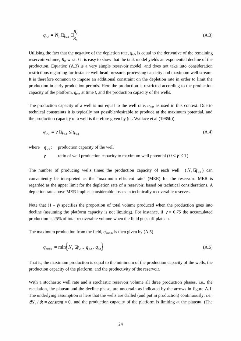
Utilising the fact that the negative of the depletion rate, qr,t, is equal to the derivative of the remaining

reservoir volume, Rt, w.r.t. t it is easy to show that the tank model yields an exponential decline of the

production. Equation (A.3) is a very simple reservoir model, and does not take into consideration

restrictions regarding for instance well head pressure, processing capacity and maximum well stream.

It is therefore common to impose an additional constraint on the depletion rate in order to limit the

production in early production periods. Here the production is restricted according to the production

capacity of the platform, qp,t, at time t, and the production capacity of the wells.

The production capacity of a well is not equal to the well rate, qw,t, as used in this context. Due to

technical constraints it is typically not possible/desirable to produce at the maximum potential, and

the production capacity of a well is therefore given by (cf. Wallace et al (1985b))

� , , ,q q qw t w t w t= ⋅ ≤γ (A.4)

where � ,qw t : production capacity of the well

γ: ratio of well production capacity to maximum well potential (0 1< ≤γ )

The number of producing wells times the production capacity of each well (N qt w t⋅ � , ) can

conveniently be interpreted as the “maximum efficient rate” (MER) for the reservoir. MER is

regarded as the upper limit for the depletion rate of a reservoir, based on technical considerations. A

depletion rate above MER implies considerable losses in technically recoverable reserves.

Note that (1 - γ) specifies the proportion of total volume produced when the production goes into

decline (assuming the platform capacity is not limiting). For instance, if γ = 0.75 the accumulated

production is 25% of total recoverable volume when the field goes off plateau.

The maximum production from the field, qmax,t, is then given by (A.5)

{ }q N q q qt t w t p t r tmax, , , ,min � , ,= ⋅ (A.5)

That is, the maximum production is equal to the minimum of the production capacity of the wells, the

production capacity of the platform, and the productivity of the reservoir.

With a stochastic well rate and a stochastic reservoir volume all three production phases, i.e., the

escalation, the plateau and the decline phase, are uncertain as indicated by the arrows in figure A.1.

The underlying assumption is here that the wells are drilled (and put in production) continuously, i.e.,

∂ ∂N t constantt / = > 0, and the production capacity of the platform is limiting at the plateau. (The

25

plateau level is uncertain because the reservoir productivity may fall below the platform capacity, due

to a drop in the well rate.)

If the platform capacity is not limiting, the production profile can still have a plateau level. This

happens if the drilling of production wells are completed some time before the productivity of the

reservoir becomes the limiting capacity. Then, due to the ratio γ, the production capacity of the wells

will determine the maximum production from the field and establish a temporary plateau level.

p,tq

t

?

?

?

?

?

?

? ?

Fig. A.1 General production profile for the tank model with stochastic parameters.

The foundation for the tank model implies that each reservoir volume has a unique decline rate. As a

consequence the operator learns the true reservoir volume when the production leaves the plateau and

starts to decline. Note that without restrictions on the production capacity of the wells, i.e., γ = 1, this

will happen immediately after start of production if the platform capacity is not limiting. By setting γless than 1 a plateau level is enforced, and a time lag for the unveiling of the true reservoir volume is

provided.

26

Appendix B

• Financial data

Annual rate of return: 7 %

Initial oil price: 18 USD/barrel

Parameters of the geometric Brownian motion:

drift rate, α: 0volatility, σ: 0.2

• Reservoir related data

A priori probability distribution of reservoir volume:

Volume [million Sm3]: 2 6 12Probability: 0.3 0.5 0.2

A priori probability distribution of well rate:

Well rate [million Sm3/year]: 0.53 1.60Probability: 0.5 0.5

The ratio of well production capacity to maximum well potential, γ = 0.75

Probability of a shift in well rate (between production periods): 10%

Possible production well combinations: 2,3,4,5,6

Maximum number of exploration wells: 1

Conditional probability of exploration well information:

Pr (information = “low volume” | reservoir volume is 2 million Sm3/year): 0.60Pr (information = “low volume” | reservoir volume is 6 million Sm3/year): 0.50Pr (information = “low volume” | reservoir volume is 12 million Sm3/year): 0.40

The indication obtained from the well is rather uncertain, and corresponds to one possible well

location at the field. The low content of information from the well is chosen deliberately in order to

facilitate the analysis of the qualities of the model.

• Concepts

A small or a large platform, according to the platform’s initial production capacity can develop the

field. Each platform can have three designs, specified by the possibility to increase the production

capacity after the engineering and construction phase is completed. The three designs are; no

possibility for subsequent capacity expansions, the possibility to increase the capacity in one step, and

the possibility to increase the capacity in two steps. For the considered platforms each step is 0.8

million Sm3/year.

27

Capacity, initial and potential, of platforms [million Sm3/year]:

Initial capacityInitial capacity

+ 1 step increaseInitial capacity

+ 2 steps increaseSmall platform: 0.8 1.6 2.4

Large platform: 1.6 2.4 3.2

• Investments and operating costs

Both platforms are assumed leased, and the construction cost is therefore limited to the cost of

required modifications. The construction/modification costs are given below.

Platform modification costs, small platform:

Possible capacity increase [million Sm3/year]: 0 0.8 1.6Modification costs [USD million]: 54 72 91

Platform modification costs, large platform:

Possible capacity increase [million Sm3/year]: 0 0.8 1.6Modification costs [USD million]: 100 106 117

Cost of increasing the platform’s capacity by one step (0.8 million Sm3/year): USD 38 million

Cost of increasing the platform’s capacity by two steps (1.6 million Sm3/year): USD 76 million

Fixed operating costs, small platform:

Installed capacity [million Sm3/year]: 0.8 1.6 2.4Fixed operating costs [USD million]: 24 26 28

Fixed operating costs, large platform:

Installed capacity [million Sm3/year]: 1.6 2.4 3.2Fixed operating costs [USD million]: 30 31 32

Variable production costs (including transportation): 2 USD/barrel.

Cost of drilling a production well (including well completion): USD 17 million

Cost of drilling an exploration well: USD 15 million

Production system costs11: USD 38 million

Abandonment cost (before contract is made for platform): USD 0.15 million

Abandonment cost (after contract is made for platform): USD 3 million

Cost of plugging a production well: USD 3 million

Sales value of subsea template: USD 9 million

11 Installation of a subsea template, offshore loading facilities, control systems, installation costs.