real-space pairing in an extended t j modelth- · standardowa metoda typu pola ´sredniego dla...
TRANSCRIPT

Real-space pairing in an extended t-J model
Jakub Jedrak
Rozprawa doktorska
Promotor: Prof. dr hab. Jozef Spa lek
Uniwersytet Jagiellonski
Instytut Fizyki im. Mariana SmoluchowskiegoZak lad Teorii Materii Skondensowanej i Nanofizyki
Krakow, kwiecien 2011

Abstract
High-temperature superconductivity in copper oxides (cuprates, e.g. La2−xSrxCuO4,YBa2Cu3O6+δ or Bi2Sr2CaCu2O8+δ) remains among the most spectacular phenomenain condensed matter physics. Since its discovery in 1986, an enormous number (∼ 105)of papers on the subject have appeared. So far, there is no single, commonly acceptedtheory of high-temperature superconductivity. However, it is widely believed that a basicdescription of this phenomenon can be provided by a single-band Hubbard model or itsderivative, the t-J model. The latter model is regarded as a minimal microscopic model,capable of describing the essential aspects of the complex physics of the cuprates.
Unfortunately, in general case, neither of those two models can be solved exactly andtherefore various approximate methods are used. Among them, the so-called mean-fieldmethods provide a simple, yet fairly reasonable description of the cuprates. In particular,some of the main qualitative features of the phase diagram and the essential features ofelectronic spectrum are roughly reproduced.
A standard mean-field approach to the t-J model, known under the name of renor-malized mean-field theory (RMFT) goes beyond the Hartree-Fock approximation. Conse-quently, its fully consistent treatment requires a novel theoretical approach. This has beenour original motivation to develop a general approach to the mean-field models, which isbased on the maximum entropy (MaxEnt) principle. The method is presented in detailin Part II of this Thesis, and in Part III it is applied to study RMFT of the t-J model.First, we compare the results obtained within our formalism with those of the frequentlyused non-variational approach based entirely on the self-consistent equations. Also, vari-ous versions of RMFT are compared, and the most satisfactory of them is selected. Thisoptimal version is subsequently used to study different versions of the original t-J Hamil-tonian. As a result, upper critical concentration and doping dependence of the selectedphysical quantities (e.g. the superconducting gap and the Fermi velocity) is determined atlow temperatures and in the absence of external magnetic field. We compare our findingsboth with theoretical results obtained from the Variational Monte Carlo (VMC) methods,as well as with the experimental data for selected cuprates. We show that the version ofRMFT approach formulated in this Thesis provides a reasonable qualitative and in somecases semiquantitative rationalization of the principal characteristics of the hole-dopedhigh-temperature superconductors at the optimal doping and in the overdoped regime.
Possible extensions of the proposed analysis are mentioned at the end.
Keywords: High-Tc superconductivity, cuprates, phase diagram for high-Tc compounds, strongly
correlated fermions, resonating valence-bond (RVB) state, t-J model, Gutzwiller projection, Gutzwiller
approximation, Maximum Entropy (MaxEnt) principle, mean field theory.
Streszczenie
Nadprzewodnictwo wysokotemperaturowe w tlenkach miedzi (krotko: miedzianach, np. La2−xSrxCuO4,
YBa2Cu3O6+δ lub Bi2Sr2CaCu2O8+δ) pozostaje jednym z najbardziej spektakularnych zjawisk w
fizyce materii skondensowanej. Od jego odkrycia w roku 1986, ukaza la sie ogromna liczba (∼ 105) prac
poswieconych tej tematyce. Do tej pory nie istnieje jedna, powszechnie akceptowana teoria nadprze-
wodnictwa wysokotemperaturowego. Niemniej jednak, uwaza sie prawie powszechnie, iz prawid lowy
opis tego zjawiska mozna uzyskac w ramach jednopasmowego modelu Hubbarda lub wywodzacego sie
zen modelu t-J . Ten ostatni jest uwazany takze za minimalny model mikroskopowy, zdolny opisac
istotne aspekty struktury stanow elektronowych i zwiazanej z nia z lozonej fizyki zwiazkow na bazie
tlenku miedzi.
Niestety, w ogolnym przypadku, zadnego z wyzej wymienionych modeli nie mozna rozwiazac w
sposob scis ly, i dlatego tez uzywa sie roznych metod przyblizonych. Miedzy innymi, tzw. metody pola
sredniego stanowia rozsadny kompromis pomiedzy prostota opisu a jego dok ladnoscia. W szczegolnosci,
z grubsza odtworzone zostaja g lowne cechy diagramu fazowego, a takze struktura elektronowa nad-
przewodnikow na bazie tlenku miedzi.
Standardowa metoda typu pola sredniego dla modelu t-J , znana pod nazwa zrenormalizowanej
teorii pola sredniego (ang. renormalized mean-field theory, RMFT), wykracza poza przyblizenie
Hartree-Focka. Z tego powodu, w pe lni wewnetrznie spojne potraktowanie zrenormalizowanej teorii
pola sredniego wymaga nowego podejscia teoretycznego.
Idea takiego podejscia stanowi la w tej rozprawie motywacje do rozwiniecia ogolnego podejscia
do metod typu pola sredniego, podejscia opartego na zasadzie maksimum entropii, (MaxEnt) (ang.
maximum entropy principle). Podejscie to jest szczego lowo przedstawione w czesci II rozprawy, zas w
czesci III zostaje zastosowane do badania zrenormalizowanej teorii pola sredniego dla modelu t-J . W
czesci III zaczynamy od porownania wynikow otrzymanych w ramach naszego formalizmu z wynikami
czesto uzywanego podejscia niewariacyjnego, opartego w ca losci na tzw. rownaniach samouzgod-
nionych Bogoliubowa-de Gennesa. Porownane zostaja takze rozne wersje RMFT, a nastepnie jedna z
nich, o najbardziej z punktu widzenia eksperymentu zadowalajacych w lasnosciach, zastosowana jest
do badania roznych wersji pe lnego Hamiltonianu t-J . W rezultacie, w temperaturach bliskich zera
bezwzglednego i przy braku zewnetrznego pola magnetycznego, wyznaczona zostaje gorna koncentracja
krytyczna i zaleznosci wybranych w lasnosci fizycznych (np. przerwy nadprzewodzacej oraz predkosci
Fermiego) od stopnia domieszkowania uk ladu. Nasze wyniki teoretyczne sa nastepnie porownane z
wynikami podejscia typu ’Variational Monte Carlo’ (VMC), a takze z danymi doswiadczalnymi dla
wybranych miedzianow. Pokazujemy, iz wersja RMFT sformu lowana w tej rozprawie prowadzi do
rozsadnego opisu g lownych cech wysokotemperaturowych nadprzewodnikow miedziowych domieszko-
wanych dziurowo, oraz jakosciowej, a w pewnych przypadkach po lilosciowej, zgodnosci z doswiadcze-
niem, tak przy domieszkowaniu optymalnym, jak i wiekszym od optymalnego.
Mozliwe uogolnienia zaproponowango tu podejscia sa przedstawione na koncu rozprawy. Poza
tym, w ca lej rozprawie staramy sie omowic krytycznie zasadnicze cechy opisywanego podejscia.
Contents
List of frequently used abbreviations 10
List of frequently used symbols 11
I Introduction 13
1 High-temperature superconductivity of cuprate compounds and its basic the-oretical models 131.1 General characteristics . . . . . . . . . . . . . . . . . . . . . . . . . . . . . . . . 13
1.1.1 Microscopic models of electronic states . . . . . . . . . . . . . . . . . . . 141.1.2 Resonating valence bond (RVB) state . . . . . . . . . . . . . . . . . . . . 14
1.2 Mean-field description of high-Tc superconductors . . . . . . . . . . . . . . . . . 151.2.1 Slave-boson theories of the t-J model . . . . . . . . . . . . . . . . . . . . 161.2.2 RMFT versus VMC method . . . . . . . . . . . . . . . . . . . . . . . . . 171.2.3 Nonstandard character of RMFT approach . . . . . . . . . . . . . . . . . 17
2 Aim and a scope of the Thesis 18
II Application of maximum entropy principle to mean-field mod-els 20
3 Synopsis: qualitative aspects of mean-field theory 203.1 General remarks on mean-field approach . . . . . . . . . . . . . . . . . . . . . . 20
3.1.1 Introductory remarks . . . . . . . . . . . . . . . . . . . . . . . . . . . . . 203.1.2 Spontaneous symmetry breaking . . . . . . . . . . . . . . . . . . . . . . . 203.1.3 Landau theory . . . . . . . . . . . . . . . . . . . . . . . . . . . . . . . . 213.1.4 Mean-field approach as a semi-classical description . . . . . . . . . . . . 213.1.5 MF formalism as a result of saddle-point approximation . . . . . . . . . . 233.1.6 Mean-field approach as a description based on restricted class of quantum
observables . . . . . . . . . . . . . . . . . . . . . . . . . . . . . . . . . . 233.1.7 Statistical mechanics and spontaneous symmetry breaking . . . . . . . . 233.1.8 Method of quasi-averages . . . . . . . . . . . . . . . . . . . . . . . . . . . 243.1.9 ’More is different’ . . . . . . . . . . . . . . . . . . . . . . . . . . . . . . . 24
3.2 How to solve mean-field models? . . . . . . . . . . . . . . . . . . . . . . . . . . . 253.2.1 Variational principle based on Bogoliubov-Feynman inequality and its
generalizations . . . . . . . . . . . . . . . . . . . . . . . . . . . . . . . . 253.2.2 Mean-field description involving only a mean-field Hamiltonian . . . . . . 253.2.3 Approach based on Bogoliubov-de Gennes equations . . . . . . . . . . . . 263.2.4 Maximum entropy principle . . . . . . . . . . . . . . . . . . . . . . . . . 263.2.5 Optimal effective mean-field picture . . . . . . . . . . . . . . . . . . . . . 273.2.6 Zero temperature situation . . . . . . . . . . . . . . . . . . . . . . . . . . 27
3.3 Summary of synopsis . . . . . . . . . . . . . . . . . . . . . . . . . . . . . . . . . 27
4 Formalism and method 294.1 Mean-field Hamiltonian . . . . . . . . . . . . . . . . . . . . . . . . . . . . . . . 294.2 MaxEnt principle and statistical mechanics . . . . . . . . . . . . . . . . . . . . . 304.3 Maximum entropy principle in the context of mean-field theory . . . . . . . . . . 31
4
4.3.1 Mean-field density operator and self-consistency conditions . . . . . . . . 314.3.2 Incomplete treatment . . . . . . . . . . . . . . . . . . . . . . . . . . . . . 314.3.3 An attempt to eliminate mean-fields . . . . . . . . . . . . . . . . . . . . 324.3.4 Complete treatment: method of Lagrange multipliers . . . . . . . . . . . 324.3.5 Trivial time dependence of equilibrium mean-field Hamiltonian and den-
sity operator . . . . . . . . . . . . . . . . . . . . . . . . . . . . . . . . . 334.4 Explicit form of mean-field density operator and the optimal (equilibrium) values
of mean fields . . . . . . . . . . . . . . . . . . . . . . . . . . . . . . . . . . . . . 344.4.1 Variational parameters of a non- mean-field character . . . . . . . . . . . 354.4.2 Explicit form of functional dependence of mean-field density operator on
~A,~λ and ~b variables . . . . . . . . . . . . . . . . . . . . . . . . . . . . . . 364.4.3 Generalized grand potential . . . . . . . . . . . . . . . . . . . . . . . . . 364.4.4 Grand-canonical (equilibrium) mean-field Hamiltonian and density operator 374.4.5 Approach based solely on Bogoliubov-de Gennes self-consistent equations 38
4.5 Non-equilibrium situation and relation of the present approach to Landau theoryof phase transitions . . . . . . . . . . . . . . . . . . . . . . . . . . . . . . . . . . 384.5.1 Self-consistency conditions for arbitrary values of mean-fields . . . . . . . 384.5.2 Interpretation of Fz( ~A,~b) function as Landau potential . . . . . . . . . . 394.5.3 Incorrect construction of Landau potential . . . . . . . . . . . . . . . . . 404.5.4 Final remarks . . . . . . . . . . . . . . . . . . . . . . . . . . . . . . . . . 41
4.6 Equilibrium thermodynamics . . . . . . . . . . . . . . . . . . . . . . . . . . . . 414.6.1 Grand potential . . . . . . . . . . . . . . . . . . . . . . . . . . . . . . . . 414.6.2 First derivatives of grand potential . . . . . . . . . . . . . . . . . . . . . 424.6.3 Second derivatives of grand potential . . . . . . . . . . . . . . . . . . . . 434.6.4 Specific heat . . . . . . . . . . . . . . . . . . . . . . . . . . . . . . . . . . 444.6.5 Other thermodynamic potentials . . . . . . . . . . . . . . . . . . . . . . 444.6.6 Equilibrium thermodynamics: final remarks . . . . . . . . . . . . . . . . 45
4.7 Additional remarks on chemical potential . . . . . . . . . . . . . . . . . . . . . . 464.8 Equivalence classes of mean-field Hamiltonians . . . . . . . . . . . . . . . . . . 47
4.8.1 Universality classes of mean-field Hamiltonians . . . . . . . . . . . . . . . 484.8.2 Equivalence relation . . . . . . . . . . . . . . . . . . . . . . . . . . . . . 484.8.3 Special case of transformations (4.71) . . . . . . . . . . . . . . . . . . . . 494.8.4 Reduced form of mean-field Hamiltonian . . . . . . . . . . . . . . . . . . 504.8.5 Present approach and formalism of Reference [79] . . . . . . . . . . . . . 514.8.6 Generalization of transformations (4.77) to arbitrary form of mean-field
Hamiltonian . . . . . . . . . . . . . . . . . . . . . . . . . . . . . . . . . . 524.8.7 Present approach and formalism of References [162, 163, 164] . . . . . . . 534.8.8 Transformations (4.71) in presence of variational parameters of a non
mean-field character . . . . . . . . . . . . . . . . . . . . . . . . . . . . . 544.8.9 Vector character of mean-fields and Lagrange multipliers . . . . . . . . . 55
4.9 Mean-field Hamiltonians of Hartree-Fock form . . . . . . . . . . . . . . . . . . . 564.10 Relation of the present method to variational principle of Bogoliubov and Feyn-
man . . . . . . . . . . . . . . . . . . . . . . . . . . . . . . . . . . . . . . . . . . 574.11 Formalism interpretations . . . . . . . . . . . . . . . . . . . . . . . . . . . . . . 60
4.11.1 Observables with a priori known expectation values . . . . . . . . . . . . 604.11.2 Time dependence of mean-field variables . . . . . . . . . . . . . . . . . . 604.11.3 Super-selection rules . . . . . . . . . . . . . . . . . . . . . . . . . . . . . 614.11.4 Internal consistency of mean-field approach . . . . . . . . . . . . . . . . . 614.11.5 Physical and statistical aspects of MF statistical mechanics . . . . . . . . 624.11.6 Generalized entropies . . . . . . . . . . . . . . . . . . . . . . . . . . . . . 63
5
4.11.7 Lagrange multipliers as molecular fields . . . . . . . . . . . . . . . . . . . 63
5 Summary and discussion of Part II 64
III Mean-field theory of t-J model 65
6 t-J model 65
6.1 t-J Hamiltonian . . . . . . . . . . . . . . . . . . . . . . . . . . . . . . . . . . . . 65
6.2 General remarks on t-J model . . . . . . . . . . . . . . . . . . . . . . . . . . . . 66
6.2.1 Effective Hamiltonians: a broader perspective . . . . . . . . . . . . . . . 66
6.2.2 t-J model as a minimal model of cuprate superconductors . . . . . . . . 67
6.2.3 Nontrivial role of higher-order terms . . . . . . . . . . . . . . . . . . . . 67
6.2.4 Mean-field treatment of Hubbard model . . . . . . . . . . . . . . . . . . 68
6.2.5 t-J-U model . . . . . . . . . . . . . . . . . . . . . . . . . . . . . . . . . . 68
6.2.6 Other possible extensions of t-J model . . . . . . . . . . . . . . . . . . . 68
7 Renormalized mean-field theory (RMFT) 70
7.1 Concept of resonating valence bond (RVB) state and correlated variational wavefunctions . . . . . . . . . . . . . . . . . . . . . . . . . . . . . . . . . . . . . . . 70
7.2 Mean-field treatment of Gutzwiller projected state . . . . . . . . . . . . . . . . 71
7.2.1 Exact evaluation of correlated averages and rigorous upper bound forexact ground state energy . . . . . . . . . . . . . . . . . . . . . . . . . . 72
7.2.2 Projected versus unprojected quantities . . . . . . . . . . . . . . . . . . . 73
7.3 Standard formulation of renormalized mean-field theory . . . . . . . . . . . . . . 73
7.3.1 RMFT Hamiltonian . . . . . . . . . . . . . . . . . . . . . . . . . . . . . 73
7.4 Solving renormalized mean-field theory: application of MaxEnt-based variationalapproach . . . . . . . . . . . . . . . . . . . . . . . . . . . . . . . . . . . . . . . . 75
7.4.1 Finite temperature and mixed correlated states . . . . . . . . . . . . . . 75
7.4.2 Formalism of Part II: application to t-J model . . . . . . . . . . . . . . . 76
7.4.3 Alternative formulation of renormalized mean-field theory . . . . . . . . 77
7.4.4 Choice of relevant mean-fields . . . . . . . . . . . . . . . . . . . . . . . . 79
7.5 Renormalization schemes used in the present work . . . . . . . . . . . . . . . . 80
7.5.1 The simplest from of renormalization factors . . . . . . . . . . . . . . . . 80
7.5.2 Renormalization scheme of Fukushima . . . . . . . . . . . . . . . . . . . 80
7.5.3 Renormalization scheme of Sigrist et al. . . . . . . . . . . . . . . . . . . . 81
7.5.4 Renormalization scheme of Ogata and Himeda . . . . . . . . . . . . . . . 81
7.5.5 Renormalized superconducting order parameter . . . . . . . . . . . . . . 82
8 Results I: Comparison of two methods of approach and different renormal-ization schemes 83
8.1 Superconducting d-wave (dSC) solution . . . . . . . . . . . . . . . . . . . . . . . 83
8.1.1 Numerical results . . . . . . . . . . . . . . . . . . . . . . . . . . . . . . . 84
8.2 Staggered flux solution . . . . . . . . . . . . . . . . . . . . . . . . . . . . . . . . 88
8.2.1 Numerical results . . . . . . . . . . . . . . . . . . . . . . . . . . . . . . . 90
8.3 Pomeranchuk instability . . . . . . . . . . . . . . . . . . . . . . . . . . . . . . . 91
8.3.1 Numerical results . . . . . . . . . . . . . . . . . . . . . . . . . . . . . . . 92
6
9 Results II: Optimal renormalization scheme and its application to t-J model 949.1 Non-standard formulation of RMFT approach . . . . . . . . . . . . . . . . . . . 94
9.1.1 RMFT Hamiltonian . . . . . . . . . . . . . . . . . . . . . . . . . . . . . 949.1.2 Generalized Landau potential and equations (4.34) . . . . . . . . . . . . 969.1.3 Characteristics of the model: qualitative analysis . . . . . . . . . . . . . 96
9.2 Numerical results . . . . . . . . . . . . . . . . . . . . . . . . . . . . . . . . . . . 969.2.1 Hole concentration x = 0.175 . . . . . . . . . . . . . . . . . . . . . . . . 979.2.2 Doping dependence of mean-field quantities . . . . . . . . . . . . . . . . 989.2.3 Dependence of upper critical concentration on value of exchange integral
J . . . . . . . . . . . . . . . . . . . . . . . . . . . . . . . . . . . . . . . 101
10 Summary and discussion 10210.1 Summary . . . . . . . . . . . . . . . . . . . . . . . . . . . . . . . . . . . . . . . 102
10.1.1 Comparison of present variational method and non-variational approachbased on self-consistent equations . . . . . . . . . . . . . . . . . . . . . . 102
10.1.2 Comparison of different renormalization schemes . . . . . . . . . . . . . . 10210.1.3 Optimal renormalization scheme . . . . . . . . . . . . . . . . . . . . . . . 10310.1.4 Limitations of RMFT approach . . . . . . . . . . . . . . . . . . . . . . . 103
10.2 Outlook and possible extensions of present work . . . . . . . . . . . . . . . . . . 10410.2.1 Approximation-free evaluation of correlated averages . . . . . . . . . . . 10410.2.2 Other trial correlated states . . . . . . . . . . . . . . . . . . . . . . . . . 10410.2.3 Higher-order corrections to t-J Hamiltonian . . . . . . . . . . . . . . . . 10510.2.4 Analysis a nonzero temperature . . . . . . . . . . . . . . . . . . . . . . . 10510.2.5 More complex symmetry-broken states, lattice geometry, and band struc-
ture . . . . . . . . . . . . . . . . . . . . . . . . . . . . . . . . . . . . . . 10510.2.6 Ginzburg-Landau potential . . . . . . . . . . . . . . . . . . . . . . . . . . 106
IV Appendices and supplementary material 107
11 Appendices 10711.1 Appendix A: Deficiencies of approach not based on the method of Lagrange
multipliers . . . . . . . . . . . . . . . . . . . . . . . . . . . . . . . . . . . . . . . 10711.2 Appendix B: Equivalence of two alternative expressions for the second derivative
of thermodynamic grand potential Ω . . . . . . . . . . . . . . . . . . . . . . . . 10811.3 Appendix C: Generalized thermodynamic potentials and Legendre transforma-
tions . . . . . . . . . . . . . . . . . . . . . . . . . . . . . . . . . . . . . . . . . . 10911.4 Appendix D: Renormalization scheme of Fukushima . . . . . . . . . . . . . . . 110
12 Supplements 11212.1 Supplement A: Thermodynamic fluctuations and internal limitations of mean-
field description . . . . . . . . . . . . . . . . . . . . . . . . . . . . . . . . . . . . 11212.1.1 Probability of a non-equilibrium MF configuration . . . . . . . . . . . . . 11212.1.2 ’Classical’ and ’quantum’ probability distributions . . . . . . . . . . . . . 11312.1.3 Degenerate minima of Fz( ~A) . . . . . . . . . . . . . . . . . . . . . . . . . 11312.1.4 Dual nature of fluctuations . . . . . . . . . . . . . . . . . . . . . . . . . . 11412.1.5 Classical fluctuations: some definitions and notation . . . . . . . . . . . . 11412.1.6 Constant number of mean-fields . . . . . . . . . . . . . . . . . . . . . . . 11512.1.7 Spatial dependence of mean-fields: general case . . . . . . . . . . . . . . 11612.1.8 Quantum fluctuations . . . . . . . . . . . . . . . . . . . . . . . . . . . . 118
7
12.1.9 Fluctuations: summary and final remarks . . . . . . . . . . . . . . . . . . 11912.2 Supplement B: Zero temperature limit of mean-field approach . . . . . . . . . . 119
12.2.1 Introductory remarks . . . . . . . . . . . . . . . . . . . . . . . . . . . . . 11912.2.2 Assumptions . . . . . . . . . . . . . . . . . . . . . . . . . . . . . . . . . . 12012.2.3 Incomplete approach . . . . . . . . . . . . . . . . . . . . . . . . . . . . . 12012.2.4 The method of Lagrange multipliers . . . . . . . . . . . . . . . . . . . . . 12112.2.5 ~A,~λ - independent eigenstates of Hλ( ~A) . . . . . . . . . . . . . . . . . . 12212.2.6 Non-analytical minima . . . . . . . . . . . . . . . . . . . . . . . . . . . . 12212.2.7 Excited states . . . . . . . . . . . . . . . . . . . . . . . . . . . . . . . . . 12312.2.8 Summary: deficiencies of zero-temperature MF approach . . . . . . . . . 123
12.3 Supplement C: Mean-field model of the spin system as an illustrative examplefor application of the MaxEnt-based variational approach . . . . . . . . . . . . 12412.3.1 Construction of mean-field Hamiltonian . . . . . . . . . . . . . . . . . . . 12412.3.2 Free energy functional and equilibrium situation . . . . . . . . . . . . . . 12512.3.3 Non-equilibrium situation . . . . . . . . . . . . . . . . . . . . . . . . . . 12512.3.4 Limit of zero temperature . . . . . . . . . . . . . . . . . . . . . . . . . . 12712.3.5 Generalization to m-dependent exchange integral J . . . . . . . . . . . . 12812.3.6 General solution with non-uniform magnetization . . . . . . . . . . . . . 12812.3.7 Quantum fluctuations . . . . . . . . . . . . . . . . . . . . . . . . . . . . 130
References 131
8

Podziekowania
Profesorowi Jozefowi Spa lkowi, promotorowi niniejszej rozprawy, jestem bardzo wdziecznyza zaproponowanie tematyki badan, za cenne dyskusje oraz za wszelkie otrzymane uwagi,zarowno merytoryczne, jak i jezykowe. Dziekuje Mu takze za wsparcie, wyrozumia losc i cier-pliwosc, jakimi darzy mnie w ciagu wielu lat naszej wspo lpracy.
Profesorowi Krzysztofowi Rosciszewskiemu bardzo dziekuje za cenne uwagi i wskazowki,ktore otrzyma lem od Niego na wczesnym etapie pracy nad zagadnieniami przedstawionymi wniniejszej rozprawie.
Chcia lbym podziekowac Wszystkim, ktorzy w mniejszym lub wiekszym stopniu przyczynilisie do powstania niniejszej pracy swoimi radami, zacheta, uwagami i dyskusjami, jak rowniezwszelakiego rodzaju pomoca: Marcinowi Abramowi, doktorowi Andrzejowi Biborskiemu, PaniDanucie Goc-Jag lo doktorowi Micha lowi Hellerowi, Oldze Howczak, Janowi Kaczmarczykowi,doktorowi Andrzejowi Kapanowskiemu, Ma lgorzacie Kaliszan, Micha lowi K losowi, MagdalenieKoz lowskiej, Jaromirowi Krzyszczakowi, doktorowi Romanowi Marcinkowi, doktorowi Marci-nowi Raczkowskiemu, doktor Joannie Sapetowej, Zygmuntowi Starypanowi, Katarzynie Tar-gonskiej, doktorowi Krzysztofowi Wohlfeldowi oraz Marcinowi Wysokinskiemu.
Pragne takze goraco podziekowac Profesorowi Ehudowi Altmanowi i Jego Wspo lpracowni-kom, w szczegolnosci doktor Lilach Goren, za zyczliwa goscine, cenne dyskusje i krytyczne uwagijakie otrzyma lem w trakcie mojego krotkiego pobytu w Instytucie im. Chaima Weizmanna wRehovot.
Jestem bardzo wdzieczny Profesorowi Florianowi Gebhardowi i doktorowi Jorgowi Bune-mannowi, za uwagi i dyskusje, ktore mia ly miejsce podczas konferencji ’Korrelationstage 2011’w Instytucie im. Maksa Plancka w Dreznie.
Moja ogromna wdziecznosc nalezy sie rowniez Autorom biblioteki GSL (Gnu Scientific Li-brary), w oparciu o ktora wykonane zosta ly wszystkie obliczenia numeryczne przedstawione wniniejszej rozprawie.
Niniejsza rozprawa by la czesciowo finansowana z grantu (N N 202 128 736) MinisterstwaNauki i Szkolnictwa Wyzszego Rzeczpospolitej Polskiej.
9

List of frequently used abbreviations
AF antiferromagneticARPES angle resolved photoemission spectroscopyBCS Bardeen-Cooper-SchriefferFFLO Fulde-Ferrell-Larkin-OvchinnikovFS Fermi surfaceGA Gutzwiller approximationGC grand canonicalGWF Gutzwiller wave functionHF Hartree-FockMaxEnt maximum entropyMF mean-fieldPG pseudogapPI Pomeranchuk instabilityRMFT renormalized mean-field theoryRS renormalization schemeRVB resonating valence bondSBMFT slave-boson mean-field theorySC superconductingSF staggered fluxs-c self-consistentvar variational
10
List of frequently used symbols
〈A〉 average value of operator A (Eqn. (4.2))A1, A2, . . . , AM mean fields~A = (A1, A2, . . . , AM) vector of mean fields
H( ~A) ≡ H mean-field (MF) Hamiltonian (Eqn. (4.1))
DA domain of a MF model, i.e., those ~A, for which H( ~A)is well-defined
DS spatial dimension of the crystal latticeDH dimension of the Hilbert space
N particle number operatorΛ number of lattice sites
He, ρe ’exact’, i.e., non-MF Hamiltonian and the correspondingdensity operator (Eqn. (4.6))
µ, T , β = 1/kBT chemical potential, temperature and inverse temperatureSe entropy functional for ρe (Eqn. (4.3))SvN (ρ) von Neumann entropy for density operator ρ (Eqn. (4.4))S MF entropy functional (Eqn. (4.9))∑M
s=1 λs(Tr[ρλAs] − As) self-consistency preserving constraints (Eqn. (4.13))λ1, λ2, . . . , λM Lagrange multipliers~λ = (λ1, λ2, . . . , λM) vector of Lagrange multipliersSλ MF entropy functional S (4.9) supplemented with
the self-consistency-preserving constraints (Eqs. (4.14), (4.21)).
Hλ = H −∑Ms=1 λs(As −As) H( ~A) (4.1) supplemented with the constraint terms (Eqn. (4.15))
Kλ ≡ Hλ − µN MF grand Hamiltonian corresponding to Hλ (Eqn. (4.16))
ρλ = Z−1λ exp
(
− βKλ
)
MF density operator (Eqn. (4.29))
Z−1λ = Tr[exp
(
− βKλ
)
] MF partition function (Eqn. (4.29))pi, qi probability of i-th microstateb1, b2, . . . , bP variational parameters of a non-MF character
(b1, b2, . . . , bP ) ≡ ~b vector of bl parameters
F( ~A,~λ,~b) ≡ −β−1 lnZλ( ~A,~λ,~b) generalized grand potential (Eqn. (4.33))~A0, ~λ0, ~b0 optimal (equilibrium) values of ~A, ~λ, and ~b, respectively
Kλ0 = Kλ( ~A0, ~λ0,~b0) equilibrium MF grand Hamiltonian (Eqn. (4.36))
ρλ0 = Z−1λ0 exp(−βKλ0) equilibrium (canonical) MF density operator (Eqn. (4.37))
~A(0)sc Optimal solution of the self-consistent equations obtained
within the non-variational approach (Eqn. (4.38))~λ( ~A) solution of the self-consistent equations obtained within
the approach proposed in the present Thesis (Eqn. (4.41))
Hz( ~A) ≡ Hλ( ~A,~λ( ~A)) self-consistent MF Hamiltonian (Eqn. (4.42))
ρz( ~A) = ρλ( ~A,~λ( ~A)) self-consistent MF density operator (Eqn. (4.43))
Fz( ~A,~b) ≡ F( ~A,~λ( ~A,~b),~b) Landau potential (Eqn. (4.44))
Ω(T, V, µ,~h) thermodynamic grand potential (Eqn. (4.47))
F (T, V,N,~h) = Ω + µN free energy (Helmholtz free energy) (Eqn. (4.58))
11
~Ri position vector of the i-th lattice site
|~Ri − ~Rj | = d(i, j) distance between i-th and j-th lattice sites
HtJ Hamiltonian of the t-J model (Eqs. (6.127), (6.132), (6.136))
Ht kinetic energy part of the t-J Hamiltonian
HJ exchange part of the t-J Hamiltonian (Eqn. (6.128))
H3 three-site term part of the t-J Hamiltonian (Eqn. (6.130))
HtU Hubbard Hamiltonian (Eqn. (6.133))
HtJU t-J-U Hamiltonian (Eqn. (6.137))
tij hopping integral between lattice sites labeled by ~Ri and ~Rj
Jij exchange integral between lattice sites labeled by ~Ri and ~Rj
P =∏
i(1 − ni↑ni↓) Gutzwiller projection operator (Eqn. (6.129))|BCS〉 Bardeen-Cooper-Schrieffer (BCS)-type state (Eqn. (7.139))
|RVB〉 = P |BCS〉 resonating valence bond state (Eqn. (7.138))
|Ψ〉 = PC |Ψ0〉 general correlated trial state (Eqn. (7.140))
PC general correlation operator (correlator)|Ψ0〉 eigenstate of some single-particle Hamiltonian
〈O〉C ≡ 〈Ψ|O|Ψ〉/〈Ψ|Ψ〉 correlated average of operator O (Eqn. (7.145))
〈O〉 ≡ 〈Ψ0|O|Ψ0〉 uncorrelated average of OgO renormalization factor for operator O (Eqn. (7.148)).gt
ij renormalization factor for the kinetic energygJ
ij renormalization factor for the spin exchange interactionρ0 grand canonical single-particle mixed state
ρC = PC ρ0PC correlated mixed state
HR RMFT Hamiltonian (Eqn. (7.153))
HRλ RMFT Hamiltonian supplemented with the constraint terms (Eqn. (7.164))
H(∼)R = W (χijσ,∆ij , niσ)1DH
alternative form of HR
H(∼)Rλ alternative form of HRλ (Eqn. (7.165))
W (χijσ,∆ij, niσ) = 〈HR〉 = 〈He〉appC exact expectation value of HR
(approximate expectation value of He)
χijσ ≡ 〈c†iσcjσ〉 hopping amplitude (bond order parameter)∆ij ≡ 〈ciσcjσ〉 = 〈cjσciσ〉 superconducting gap parameter
∆Cij ≡ 〈∆ij〉C superconducting order parameter
c†iσ (ciσ) creation (annihilation) operator for electron with spin σ = ±on the site labeled by ~Ri
n = 〈N〉/Λ = N/Λ average number of electrons per lattice sitex = 1 − n hole dopingk quasimomentumξk quasiparticle energy in the normal state (Eqn. (9.215))Dk superconducting gap (Eqn. (9.215))Ek quasiparticle energy (Eqn. (9.215))vF Fermi velocity (Eqn. (9.221))
12
Part I
Introduction
1 High-temperature superconductivity of cuprate com-
pounds and its basic theoretical models
1.1 General characteristics
High-temperature (high-Tc) superconductivity, in particular that of the cuprate compounds(cuprates)1, is one of the most puzzling and challenging subjects in condensed matter physics[1, 2, 4, 5, 6, 7, 8]. Since its discovery by Bednorz and Muller in 1986 [9], there is still a largeinterest in this field. It is partly due to potentially revolutionary technological applications - formost of high-Tc cuprate compounds the critical temperature (Tc) exceeds 77K, i.e., the boilingtemperature of liquid nitrogen. From the point of view of a physicist, cuprates are exciting dueto their complex structure and unusual properties.
We should mention right at the beginning that it is not our aim here to analyze in detailthe large number of the existing experimental data for the cuprates. Rather, we invoke onlythe basic facts and focus on properties, which can be described or even predicted by simpletheoretical models and methods we use.
A number of high-Tc cuprate compounds have been discovered. The most notable areLa2−xSrxCuO4 (LSCO), with the maximal critical temperature Tc (which however depends onthe hole doping x) equal 36K, YBa2Cu3O6+δ (YBCO) with Tc ≤ 91K, and Bi2Sr2CaCu2O8+δ
(BSCCO or more precisely, Bi2212) with Tc ≤ 89K [2]. As suggested by their chemical for-mulas, all cuprate compounds have one or more CuO2 plains, separated by atoms of otherelements. All exhibit strong tetragonal anisotropy in the c-axis direction, and their quasi-twodimensional structure seems to be responsible for many of the essential properties of those ma-terials. Additionally, for some high-Tc compounds, a weaker in-plane anisotropy between a andb axes may appear (orthorhombic structure). The doping-temperature (x-T ) phase diagram ofall hole-doped2 high-Tc compounds (cf. Fig. 1) have a similar structure [1, 2, 4, 8]. Upon thehole doping, with the hole concentration x & 0.02−0.05, a generic antiferromagnetic (AF) Mottinsulating state of the undoped parent compound [10, 11] eventually transforms (for x ≈ 0.05)into a superconducting (SC) state of a dx2−y2 (d-wave) symmetry [12]. Still, even in absenceof the long-range antiferromagnetic (AF) order, the antiferromagnetic correlations seem to bepresent in the SC state. The latter, in turn, after reaching a maximal transition temperatureat x ≈ 0.15−0.2, disappears at the upper critical concentration xc ≈ 0.25−0.35, depending onthe compound [13, 14]. In the overdoped regime x & 0.15 − 0.2 the system evolves graduallyfrom a non-Fermi liquid into a quantum liquid that can be regarded as an unconventional Fermiliquid [15].
The region of the x-T phase diagram where superconductivity appears is called a ’dome’due to its characteristic shape. For some cuprate compounds, antiferromagnetic and supercon-
1Apart from the cuprates, the class of high-temperature superconductors encompasses also the recentlydiscovered iron-based superconductors, like pnictides, e.g. Ba1−xKxFe2As2 or oxypnictides, e.g. GdFeAsO0.85.It should be also noted, that organic superconductors, e.g. (TMTSF)2PF6, although having Tc ∼ 1 − 10K,share many properties with both copper and iron superconductors [4].
2There exist also electron-doped high-Tc cuprate compounds, e.g. Nd2−xCexCuO4 (Tc = 23K). The genericx-T phase diagram of electron-doped compounds exhibits remarkable quantitative differences as compared tothat of its hole-doped counterpart [2, 3]. Although here we concentrate on the hole-doped case, please notethat essentially the same theoretical methods which are developed in this Thesis may also be used to study theelectron-doped compounds.
13

La Sr CuO2–x x 4
non-Fermi liquid
Tp
Tcte
mp
era
ture
pseudogap
an
tife
rro
ma
gn
etic
superconducting
Fermi liquid
0 0.02 0.06 0.2 0.32
doping level (holes per CuO )2
underdoped optimally doped overdoped
Figure 1: Schematic hole doping (x) - temperature (T ) phase diagram of La2−xSrxCuO4, takenas an example of a generic hole-doped cuprate superconductor. The vertical solid line marksqualitatively the division into underdoped and the overdoped regimes.
ducting orders occur simultaneously, i.e., we have the AF-SC phase coexistence. For others,the AF and SC regions of the phase diagram are separated by a disordered (’glassy’) state.
Finally, one of the most intriguing features of the cuprates is the existence of an unconven-tional normal state, called ’pseudogap’ (PG) or ’spin gap’ [6, 8]. Pseudogap phase is visible invarious experiments [16, 17, 18] above the superconducting dome in the underdoped regime.In this phase, the gaped behavior in the temperature dependence of the NMR relaxation rateis observed [8]. Also, both NMR and ARPES experiments show that magnetic excitations aresuppressed in the temperature range Tc < T < T ∗, and that the energy gap is gradually formedin one-particle excitations below T ∗. The pseudogap behavior is often interpreted as an offsetof the pre-formed pairs with the dx2−y2 -like quasimomentum (k) -dependence as in the SCphase [8].
1.1.1 Microscopic models of electronic states
In order to provide a theoretical description of the cuprate superconductivity, the Hubbardmodel is often invoked. Both the simplest, single-band form [19, 20, 21], as well as the morerealistic three band (d-p model, see [8] and References therein) are used. The former modelresults from ascribing a passive role to the electrons on px and py oxygen orbitals and retainingonly the dynamics of electrons on the copper 3dx2−y2 orbitals. In the strong-coupling limit (i.e.,with the Coulomb interaction dominant over the kinetic energy of the electrons), the single-band Hubbard model can be transformed into the t-J model [8, 22, 23, 24, 25, 26, 27, 28, 29,30, 31], which is often regarded as a minimal, purely electronic microscopic model of high-Tc
superconductivity. Unfortunately, as for the most of the realistic models of interacting electrons,exact solutions of the t-J model are limited to very special choice of the model parameters or tovery small clusters [32]. Consequently, approximate methods of various kinds must be invoked.
1.1.2 Resonating valence bond (RVB) state
A theoretical concept which also seems to be important for the description of high-Tc supercon-ductivity is that of the resonating valence bond (RVB) state [33]. As mentioned in the latterReference, the notion of resonating valence bonds has been introduced by Pauling in the early
14
years of quantum chemistry [34, 35], e.g. to explain the nature of the electronic structure ofbenzene. In condensed matter physics, the RVB state has been originally used as a possiblevariational ground state of the Heisenberg Hamiltonian on frustrated lattices [36, 37]. Later,it has been proposed by Anderson [38] (cf. also Refs. [39, 40]) as a candidate for the groundstate of a generic strongly-correlated two-dimensional superconductor.
RVB state is a coherent superposition of electron spin-singlets residing on different pair ofsites (bonds); hence the name. Due to the lack of the long-range magnetic order, it is an exam-ple of a spin-liquid state. On the other hand, RVB state is a Bardeen-Cooper-Schrieffer (BCS)state [41, 42, 43, 44] with doubly occupied configurations in the real space being excluded viathe so-called Gutzwiller projection [8, 20, 33]. In other words, RVB state may be expected toplay (at least to some extent) a similar role for a description of the high-Tc superconductors,as its uncorrelated counterpart, i.e., the BCS state plays in the theory of conventional super-conductivity. The original RVB state may be generalized in several ways, e.g. by including thecorrelation effects in a more sophisticated manner or by implementing more complex patternsof the symmetry breaking [8, 33].
In one dimension (DS = 1), at the half-filling (x = 0), a chain of singlets has lower energythan the Neel antiferromagnetic state. For DS = 2 this is no longer the case; simple ’static’singlet covering yields the energy higher than the antiferromagnetic state, nevertheless, the trueRVB state remains competitive to the Neel-ordered state [33]. Consequently, in two dimensions,the RVB state seems to be a reasonable variational Ansatz for the ground state of t-J andrelated models. On the technical level, this idea may be realized in two different ways. First,the expectation value of any operator (in particular, of the t-J Hamiltonian) in the RVB statemay be computed by means of the Variational Monte Carlo (VMC) method [45, 46, 47, 48,49, 50, 51, 52, 53, 54, 56, 57]. Alternatively, RVB picture may be implemented by using anappropriate form of the mean-field (MF) approach.
1.2 Mean-field description of high-Tc superconductors
In this Thesis, we focus on a particular mean-field (MF) approach to the t-J model, knownunder the name of the renormalized mean-field theory (RMFT) [8, 33, 58]. RMFT is an effectof applying Gutzwiller approximation (GA) [20, 59, 60], originally devised for the Hubbardmodel, to the t-J model. The resulting single-particle picture is widely used due to its ’clarityand directness’ [39, 61]. Moreover, RMFT is capable of reproducing the basic qualitative, andeven some quantitative features of phase diagram of the cuprates [8, 33, 39]. This may be quitesurprising, because in contrast to conventional superconductors, such as Al, Sn or Pb, welldescribed by the BCS theory of a mean-field character, for the cuprates the MF approximationseems to be less adequate, for the following reason. Namely, conventional superconductors arecharacterized by a large coherence length. Therefore, the average distance between Cooperpairs is much smaller then the pair size (∼ 1000A), and each pair is immersed in, and interactswith many other pairs. This is the physical cause of the striking success of the Hartree-Fockapproximation and BCS theory in those systems. On the other hand, high-Tc cuprates arecharacterized by a small coherence length, the average pair size is in the range ∼ 10− 30A [7],i.e., it is only moderately greater then the average distance between electrons in the CuO2 plane.For that reason, some authors even argue, that no theory of a mean-field type is applicable tocuprates. For example, Kadanoff [132] states that the mean-field theory ”does not work for high-Tc superconductors”. In our opinion, however, this means only that we cannot invoke the samephysical arguments for the validity of the MF approach as in the case of BCS superconductors,and MF treatment of the cuprates requires an alternative justification.
The basic question is then whether we can regard RMFT as a satisfactory theoretical de-scription of high-Tc compounds, despite its simplistic nature and apparent shortages. This point
15
of view has been advocated strongly by Anderson and coworkers [39, 40, 61], and RMFT hasbeen, and still is, widely used in studies of the cuprates, cf. e.g. [33, 40, 58, 60, 61, 62, 63, 64,65, 66, 67, 68, 69, 70, 71, 72, 73, 74, 75, 76, 77, 78, 79, 80, 81, 82, 83, 84]. However, it has beenalso pointed out that RMFT can be placed in the Fermi-liquid paradigm (cf. e.g. [59, 85]), and,as such, is not expected to provide a correct description of the whole x-T phase diagram of thecuprates, but may work well around and above the optimal doping [86]. Intuitively, with theincreasing doping, charge carriers (holes) become more mobile, and single particle descriptionshould work better. On the other hand, with the decreasing doping, charge fluctuations aresmaller, and eventually vanish in the Mott-insulating limit (x = 0). Consequently, one mayexpect large phase fluctuations in the wave function describing the superconducting groundstate. However, phase fluctuations are not included in the standard RMFT approach. Finally,similarly to the original approach of Gutzwiller, RMFT is devised only for T = 0.
Nonetheless, let us note that RMFT possess two generic properties of the MF approach,which turn to be important also for the description of the cuprates. Namely, first, it allowsfor a natural and relatively simple description of various coexisting or competing symmetry-broken states, which are encountered in the cuprates. Stripe phases [73, 74, 75] or valence-bond solid [78] are good examples of the complex symmetry broken patterns that can bedescribed within RMFT. Second, within this independent-particle picture, a Fermi surface(FS) appears in a natural manner, and the single-particle spectral properties can be easilyaddressed. Interestingly, the notion of the Fermi surface, being one of the most importantconcepts in solid state physics, is not limited to the non-interacting or weakly interactingsystems. It is known from numerous photoemission experiments [87, 88, 89, 90, 91, 92, 93],that FS or FS-like structures are present in the cuprates, despite the presence of strong electroncorrelations.3
The important question is how to modify the basic form RMFT in order to reproduce moreaccurately the physical properties of the cuprates. Several attempts to improve the originalformulation of RMFT have been made, cf. e.g. [63, 66, 71, 76].
1.2.1 Slave-boson theories of the t-J model
At this point we ought to mention another type of the MF approach, which is frequently usedin the context of the t-J model, namely that based on the slave-boson formalism, i.e., theslave-boson mean-field theory (SBMFT). Historically, SB approach in general, and SBMFT inparticular, where applied to the t-J model as early as in 1987 by Baskaran, Zou, and Anderson[94], by Baskaran, Anderson, Hsu and Zou [95], and Baskaran and Anderson [96], and laterby Kotliar and Liu [97], and Suzumura, Hasegawa, and Fukuyama [98]. SMBFT techniquesgained popularity, and those early papers were soon followed by many Authors.
Similarly to the RMFT, SBMFT provides a simple way for implementation of the RVBconcept. Also, most versions of SBMFT lead to the predictions similar to those of the simplestrealizations of RMFT approach. Moreover, the standard SBMFT approach is in fact equivalentto the properly treated corresponding version of RMFT, as discussed in Refs. [99, 100, 101]and also recently [102].4 SBMFT is apparently a finite-temperature approach, in contrast to
3We should rather say that the results of ARPES measurement may be consistently interpreted in terms ofFS existence, e.g. by fitting the tight binding dispersion relation to the experimental data.
4Strictly speaking, this is the case for the RMFT [59] and the corresponding SBMFT [103] for the Hubbardmodel. In case of the t-J model, some differences between those two approaches appear, e.g. the kinetic energyis renormalized in a different way, i.e., ∼ x within SBMFT and ∼ 2x/(1 + x) within RMFT resulting fromthe simplest version of Gutzwiller approximation (GA). However, this technical detail is inessential. Whatis important here is that we can construct a MF model completely equivalent to that resulting from SBMFTwithout invoking sophisticated field-theoretic techniques and concepts (e.g. field quantization in the presenceof constraints).
16

RMFT, which was devised to examine the ground state properties of the system. Yet, RMFTmay be formally extended to T > 0, where, however, for various reasons both approachesare not expected to lead to physically meaningful results [100]. Therefore, SBMFT have noadvantage over RMFT, and will not be discussed here.
Beyond the mean-field level, slave boson models provide a valuable tool for studying stronglycorrelated systems, as they form a basis for the effective gauge theories for the cuprates andheavy fermions [104, 105, 106]. However, this topic is outside the scope of the present Thesis.
1.2.2 RMFT versus VMC method
The results of RMFT are often compared with those of VMC approach. VMC method providesa valuable tool for studying strongly-correlated systems; applied to the cuprate superconductorsit is known to yield a good semiquantitative description of the SC correlated state, cf. Refs.[45, 46, 47, 48, 49, 50, 51, 52, 53, 54, 56, 57]. Within VMC one treats the double occupancyexclusion in an essentially exact way, and hence this method is often regarded as being superiorto any MF treatment. However, properly constructed and solved RMFT may, at least inprinciple, lead to the results similar to those of the VMC. Moreover, RMFT has also someadvantages over VMC approach. First, its results are not limited to small clusters (i.e., smallnumber of lattice sites). Second, it offers an analytic insight into the physical contents of themodel and its relevance to the experiment.
1.2.3 Nonstandard character of RMFT approach
It is important to emphasize at this point, that the RMFT of the t-J model is not of the formof the standard Hartree-Fock (HF) MF approach. Therefore, a proper solution of RMFT, inparticular of its more advanced versions (cf. e.g. [63, 66, 71, 76]), constitutes a nontrivial task.For the MF Hamiltonians of the HF form (cf. Section 4.9 for the precise definition of thisterm), minimization of the appropriate MF thermodynamic potential (the ground-state energyin particular) is equivalent to the approach based on the self-consistent equations (in the theoryof superconductivity known under the name of Bogoliubov-de Gennes (BdG) equations). Thelatter express the basic requirement of the internal consistency of the mean-field model. TheBCS theory [41, 42] is a good example of this equivalence. Also, for the HF MF Hamiltonians,the solutions of the MF model (i.e., the ground states of the MF Hamiltonian, corresponding todifferent patterns of symmetry breaking) provide us with the upper bounds on exact free energy(or the ground state energy in the T → 0 limit). This is ensured by the Bogoliubov-Feynmaninequality [107] and its generalizations [108] (cf. Section 4.10).
In general, neither of the last two statements is true for the RMFT approach. First, theunwary application of the variational method, i.e., direct minimization of the MF free or ground-state energy may lead to results that differ from those obtained by solving the self-consistentBdG equations. Moreover, by applying the Gutzwiller approximation, we may obtain values ofthe energy which are lower then the exact ground state energy of the original t-J model.
In such a situation, a non-variational treatment based solely on the BdG equations is fre-quently selected [63, 68, 73, 74, 75, 78]. However, as will be discussed in detail, this way ofapproach cannot be regarded as fully satisfactory.
17

2 Aim and a scope of the Thesis
A need for a consistent treatment of RMFT motivated us to develop a general method of solvingmean-field (MF) models. Our approach is based on the Maximum entropy principle (MaxEnt)[109, 110, 111, 112], and may be regarded as a natural extension of the original formulation ofthis principle to the non-standard case of the MF approach. Construction of this formalism isthe first principal aim of the present Thesis.
The formal method of our approach is proposed in Part II, which is organized as follows.In Section 3 we comment on the origin, role and the nontrivial nature of MF methods in ageneral context. In Section 4 we present in detail the MaxEnt-based approach to MF models.In particular, in short Subsection 4.1, a notion of the MF model and MF Hamiltonian isformally introduced. Relation between the MaxEnt principle and a standard, non-MF statisticalmechanics is reminded in Subsection 4.2, whereas the application of this principle in the contextof MF statistical mechanics is discussed in Subsection 4.3. In Subsection 4.4 the optimal(equilibrium) values of mean-field variables and the correct form of the grand-canonical MFdensity operator are obtained. Next, in Subsection 4.5 we establish a conection between thepresent approach and Landau theory of phase transitions. Namely, we show how to constructLandau potential (generalized thermodynamic potential) for a given microscopic MF model.Subsection 4.6 is devoted to construction of MF equilibrium thermodynamics. In Subsection 4.7we analyze the role of chemical potential within MF description. In Subsection 4.8 we introducea notion of equivalence class of the MF Hamiltonians. This and related concepts allow us, inparticular, to reproduce formal results of other Authors within our approach. Subsection 4.9 isdevoted to the important class of Hartree-Fock MF Hamiltonians, whereas in Subsection 4.10 wecomment on relationship of the present MaxEnt-based variational principle to the variationalprinciple based on the Bogoliubov-Feynman inequality. Subsection 4.11 contains additionalremarks, which are intended to clarify certain aspects of the present formalism. Section 5contains summary of Part II.
In Part III, the results of Part II are applied to the RMFT of the t-J model. We begin withthe introduction of different forms of the t-J Hamiltonian and discussion of some of its generalproperties (Section 6). Next, in Section 7 we present various trial variational wave functionsused as approximate ground states of the t-J Hamiltonian. It is shown, that a special classof such wave functions (so-called correlated states) leads in a natural manner to an effective,single-particle mean-field description in the form RMFT.
In Section 8, on the example of the simplest form of the t-J Hamiltonian, and by usingdifferent versions of RMFT approach, we compare first the results of the present variationalapproach with those of the non-variational treatment based on Bogoliubov-de Gennes self-consistent equations. The following MF states are analyzed: nonmagnetic, homogeneous su-perconducting state of a d-wave symmetry (dSC), (cf. e.g. Refs. [33, 39, 40, 58, 66, 61, 73,74, 75, 82, 83], to mention just a few), staggered-flux non-superconducting solution (SF) (cf.e.g. [8, 33, 62, 75, 114, 115, 116, 117, 118, 119, 120, 121, 122, 123, 124]), and the so-calledPomeranchuk instability (PI) of the normal state, i.e., the spontaneous breakdown of the C4v
symmetry [33, 125, 126, 127, 128, 129, 130], cf. also Ref. [82].
On the example of those three states we show non-trivial differences between the resultsobtained by either different method, or different variant of RMFT. Next, the optimal form ofRMFT is selected and applied within the framework of our method to study various forms ofthe t-J model (Section 9). It is also shown, that by making use of the RMFT based on theoriginal formalism of Ref. [76], we can produce the results comparable to those of VMC andwhich are also in reasonable agreement with the experiment. This is the second principal aimof the present Thesis.
Some supplementary material is provided in Appendices and Supplements (Part IV). In
18
Appendix A (Subsection 11.1) we show, that in the case of mean-field models, the method ofLagrange multipliers is indispensable for application of the MaxEnt principle. In AppendixB (Subsection 11.2) we provide the proof of equivalence of two alternative formulas for thesecond derivative of the thermodynamic grand potential. In Appendix C (Subsection 11.3) weexplain the way in which different Landau potentials can be constructed for a given mean-field model. In Appendix D (Subsection 11.4) we present briefly some details of the formalismof Ref. [76]. Supplement A (Subsection 12.1) is devoted to the analysis of some aspects ofthe non-equilibrium situation, not discussed in Section 4.5. In particular, we discuss boththermodynamic and quantum fluctuations and the internal consistency of the present mean-field approach. In Supplement B (Subsection 12.2), we analyze zero-temperature formulationof the MF approach. Finally, in Supplement C (Subsection 12.3), we illustrate the formalismdeveloped in Section 4 on the example of the MF approach to Ising model.
As mentioned previously, RMFT description is not expected to be an equally legitimateapproach within the entire x-T phase diagram of the cuprates. Consequently, we focus hereonly on the low-temperature situation and on the optimally-doped and overdoped regimes whichare believed to exhibit a nonstandard, but essentially Fermi-liquid-type behavior. Therefore,we neglect any long-range magnetic order, in particular, simple antiferromagnetic (Neel) order.We also neglect any effects of the external magnetic field.
Within the model considered here, only a single CuO2 layer is treated. In most cases (withthe exception of the PI phase, analyzed in Section 8.3) we assume the presence of a discrete C4v
rotational symmetry. The superconducting order parameter ∆(kx, ky) is taken to be a singlet ofdx2−y2 symmetry, i.e., changes sign after a rotation of π/2 radians.5 Therefore, we concentraterather on generic features of the cuprates in the vicinity of the upper critical concentration xc,although attempts to obtain material-specific results (by taking appropriate values of the modelparameters) are also made. We analyze mainly the doping dependence of a gap magnitude andselected features of the quasiparticle spectrum in the superconducting state. The particularemphasis is put on xc, which value is quite correctly predicted for the realistic values of themodel parameters. This is the first such prediction within RMFT.
Although a consistent treatment of the RMFT of the t-J model was our original motivation,the formalism presented in Part II is of a general applicability, and may be used to treatwide class of the mean-field models. It has a number of advantages, not present in standardformulation of the MF theory. We hope than this method will be found useful in the condensedmatter physics or even beyond the field. A work along these lines is being continued in ourgroup.
Present Thesis is an extension of our earlier works [82, 83, 84, 113]. It contains (in amodified and refined form) main part of [113], large parts of [83] and essentially the wholematerial presented in [82]. Also, in Ref. [102] the formalism developed here has been used toshow the equivalence of the mean-field approach resulting from the Gutzwiller approximationto the Hubbard model, with the corresponding slave-boson mean-field theory.
5Despite this particular form of ∆(kx, ky), the MF Hamiltonian, and hence the thermodynamic potentials,are still C4v-symmetric.
19
Part II
Application of maximum entropyprinciple to mean-field models
3 Synopsis: qualitative aspects of mean-field theory
3.1 General remarks on mean-field approach
3.1.1 Introductory remarks
A rigorous treatment of even simple models of many interacting particles is usually too difficult.In such a situation, various approximate methods are to be developed.
We focus here on the so-called mean-field (MF) approach. Within the MF approach, theoriginal, many-body Hamiltonian is replaced by its simplified MF counterpart, which becomestractable. Instead of interacting with each other via full many-body potentials, the particles(or spins) are allowed to interact only with various ’mean fields’ of semi-classical6 character.Additionally, mean fields usually have an interpretation of average values of certain operatorsappearing in the MF Hamiltonian. Numerical values of such averages are not a priori knownand are to be determined when solving a MF model.
From a historical perspective, methods of an essentially MF character were used first byvan der Waals to derive equation of state for non-ideal gas (1873) [131, 132, 133], and next byWeiss to describe paramagnetic - ferromagnetic transition (1908) [132, 134, 135], both examplespredate modern quantum mechanics (1925-1927). Probably the best-known example of thequantum MF approach is the Hartree-Fock (HF) approximation [136, 137], which has been used,in particular, in the Bardeen-Cooper-Schrieffer (BCS) theory of superconductivity (1957) [41].However, mean-field methods (mainly in the form of the HF approximation) found numerousapplications not only in the field of solid-state physics, but also in atomic [138], high-energy[139, 140, 141], and nuclear physics [137, 142], as well as in astrophysics (cf. e.g. [143]) and inquantum chemistry [144].
MF approach is still widely used, despite the fact, that other approximate methods exist,with the help of which we are able to treat interactions in a more accurate manner. This ispartly due to the circumstance, that the MF approach is more direct and intuitive then mostof the more sophisticated methods, which usually involve a greater emphasis on numericalanalysis. Presence of explicit analytical formulas (e.g. for the ground state energy) frequentlyallows to make certain qualitative predictions, even before the MF model is completely solved.Also, MF methods are practically not limited by the system size. Therefore, MF approach isfrequently the simplest available tool at hand, even if the proper solution of the MF modelmay also turn out to be a highly nontrivial task. However, apart from relative simplicity, thereexist other, deeper and more subtle reasons determining the importance of the MF theory.This is discussed below, where we also invoke certain facts from both quantum and statisticalmechanics.
3.1.2 Spontaneous symmetry breaking
By spontaneous symmetry breaking we understand a situation, when symmetry of the actualstate of the system is lower then the symmetry of the Hamiltonian. In general, this means thatthe symmetry of the ground state is a subgroup of the total symmetry group of the Hamiltonian.
6An attempt to ascribe more precise meaning to this term will be made in what follows.
20
This concept plays a central role in many areas of modern physics [132, 133, 145, 146]. Apartfrom condensed matter physics, it is also widely used in the realm of high-energy physics andeven in cosmology [147].
To describe spontaneous symmetry breaking in a quantitative manner, Landau introduceda concept of order parameter [148, 149]. By this term we understand any physical quantity,which has nonzero value in an ordered, i.e., less symmetric phase, and vanishes on the oppositeside of the transition point or line. Magnetization (i.e., magnetic moment of a given volume ofa specimen) may serve as a good example in the case of ferromagnetic-paramagnetic transitionin the system of interacting spins.
3.1.3 Landau theory
A notion of an order parameter is fundamental for the theory of phase transitions, developedby Landau in the years 1936-1937 [148, 149]. Within this theory, generalized thermodynamicpotential is introduced, which global minimum with respect to order parameter(s) correspondsto the equilibrium situation. In contrast to ordinary thermodynamic potentials encountered instandard thermodynamics (e.g. free energy or grand potential), generalized potentials of Lan-dau theory7 may depend on some thermodynamic variable and its conjugate variable (relatedby the Legendre transformation) at the same time. For example, in the case of magneticallyordered systems, generalized potential depends on both magnetization (an order parameter)and the external magnetic field. Only after the minimization is carried out (with respect toe.g. magnetization), the conjugate variables are no longer independent, e.g. the equilibriumvalue of magnetization is a function of magnetic field (and of other thermodynamic variables,such as the volume or temperature).
Landau theory, even if soon recognized to be quantitatively inaccurate (i.e., it predicts in-correct values of the critical exponents), had a great impact on theoretical physics [132]. Itwas later generalized by Ginzburg and Landau in order to provide a description of supercon-ductivity [151]. Both Landau and Ginzburg - Landau theories in the original formulation havephenomenological character, which means that they make almost no assumptions about theunderlying microscopic picture.
However, it may be expected, that there exists a close connection between Landau orGinzburg - Landau theory and the microscopic MF models. Mean-field variables frequentlyplay the role of order parameters, and the results of microscopic MF formulation, before themean-fields optimization, are interpreted in terms of the Landau theory, cf. [146]. Also, devel-opment of Landau approach seems to have been (at least partly) motivated by the microscopicmean-field models existing at that time, e.g. the Bragg-Williams treatment (1934) of order-disorder transition in binary alloys [152]. On the other hand, following Gorkov (cf. e.g. [44]),one may start from the microscopic MF model and derive the corresponding Ginzburg-Landaufunctional by applying Green’s function technique within the BCS theory.
In the present Thesis a natural connection between phenomenological description in thespirit of Landau and Ginzburg, and the microscopic MF models will be established from adifferent perspective.
3.1.4 Mean-field approach as a semi-classical description
Apparently, there exists some relationship between spontaneous symmetry breaking and emer-gence of the classical world from the laws of quantum mechanics.8
7Here by ’Landau theory’ we always understand the theory of phase transitions, and not the theory of Fermiliquids [150]. For the latter, the full name ’Landau theory of Fermi liquids’ is always used.
8Highly non-trivial relationship between quantum and classical physics is still not resolved. There are manyattempts to solve this problem, e.g. by invoking environmental decoherence (cf. [153] and References therein).
21

Obviously, symmetries of classical, macroscopic objects are very different from those whichare present on the quantum level. Following Ref. [157], consider an example of crystallinestate. Microscopic quantum Hamiltonian describing a collection of atoms (or ions) and electronsexhibits full translational invariance, yet in crystals the full translational symmetry is broken,and the atoms can form a regular structure.9
Apart from appearance of the crystalline state, for which symmetry-breaking is evident,essentially the same situation appears in the cases of magnetic ordering or appearance of su-perconductivity. For example, let us consider Neel state, characterized by a static, long-rangeantiferromagnetic order. This state is obviously not an exact eigenstate of the HeisenbergHamiltonian (cf. (6.128) in Section 6.136 and (12.283) in Section 12.3), regarded as a minimalmicroscopic model of real antiferromagnetically ordered materials. As another example, wemay consider a ferromagnet, which may also be described by a ground state of the HeisenbergHamiltonian, with the opposite (negative) sign of the exchange integral. However, the point is,that in the absence of an external magnetic field, this ground state is highly (strictly speaking,infinitely) degenerate. By selecting a direction of the spontaneous magnetic moment we breakthe SU(2) symmetry of the quantum model.
Using the above examples, we conclude, that the standard (i.e., without the concept of thesymmetry breaking) quantum-mechanical treatment may be inconvenient, or even insufficient todescribe various symmetry-broken states of matter, frequently encountered in condensed matterphysics. Such states, whose existence is experimentally evident, do not correspond to eigenstates(or at least to unique eigenstates) selected out of the states of those quantum Hamiltonians,which are regarded as defining correct and essentially complete microscopic models of thesystems in question. Now, it should become more clear, why the symmetry-broken states aresometimes termed ’(semi-) classical’ states or ’classical condensates’ [157, 158].10 They exhibitpeculiar properties, in particular long-range order and ’rigidity’, i.e., robustness with respectto external perturbations.
Interestingly, ’classical condensates’ can be modeled using eigenstates of the appropriateMF Hamiltonians. Existence of long-range order(s) is build into such description in a naturalmanner, and existence of the ’classical domain’ is a priori assumed. This means, that whensolving a MF model, we determine the actual optimal values of mean-fields, which may indeeddiffer from zero. By doing so, we usually break some of the unitary symmetries originallypresent in the microscopic MF Hamiltonian.
Non-zero values of mean-fields may imply that there exists a finite gap in the spectrumof the MF Hamiltonian. The presence of the gap, in turn, explains the rigidity; the systemremains in the ground state despite the external perturbations, as long as the latter are weakenough (i.e., characterized by the energy scale smaller than a gap).11
Due to non-zero value of the gap, a difference between pure, single-determinant groundstate of the MF Hamiltonian, and a mixed thermal state is insignificant at low temperatures.However, mean-field models could be also used to describe the symmetry-broken states at non-zero temperature, and then obviously both the ground state, and the excited states of the MFHamiltonian are required. In the present Thesis, we propose an approach to MF models validfor arbitrary T > 0.
However, the latter point of view has been critically examined [154, 155, 156]. This fascinating topic is outsidethe scope of the present work.
9Obviously, the existence of crystals, or any other macroscopic objects localized in space, also breaks trans-lational symmetry.
10In Ref. [157] a precise distinction between classical and semi-classical states is made, but we do not followthis terminology strictly.
11It should be noted that the gap existence is not the necessary, but rather the sufficient condition for therigidity of the broken symmetry state. For example, there exist zero-gap superconductors, in which the phaserigidity of the macroscopic wave function is the principal factor.
22
3.1.5 MF formalism as a result of saddle-point approximation
There exits yet another aspect of the classical character of the MF approach. Namely, it is well-known, that the quantum-mechanical description of a single, spinless particle may be formulatedin terms of path integrals [159]. Conversely, given a quantum-mechanical propagator, we maydistinguish a stationary path, corresponding to the classical trajectory (i.e., one making theclassical action stationary). Similarly, making use of the coherent states of spin, Bose orFermi operators, one may express the partition function of a many-body system as a pathintegral [160]. Following Fradkin [161], let us consider Hubbard model as an example. Onemay apply Hubbard-Stratonovich (HS) transformation when determining the relevant partitionfunction. This step leads to an equivalent problem, expressed in terms of both fermionic andauxiliary bosonic fields. Importantly, the partition function expressed in this way is quadraticin fermionic degrees of freedom, therefore the latter can be integrated out, and one obtains aneffective (Euclidean) action in terms of auxiliary Bose fields introduced by HS transformation.It turns out, that a saddle-point approximation applied to such an effective action is equivalentto the Hartree-Fock mean-field approximation [158]. In analogy to the single-particle case,the path, singled out by means of the saddle-point approximation, is said to correspond to a’classical’ situation. This is less obvious in the case of many-body system, than for a singleparticle, but it still seems to be justified to call the Hartree-Fock approach a ’semi-classicaltheory’ [158].
Following Refs. [157, 158], we want to point out here, that it is not the weakness of theinteraction, which justifies MF approach, but rather the existence of a non-zero value of certainorder parameter(s) and a subsequent ability to include the fluctuations around the mean-fieldsolution to obtain a complete description. In other words, description in terms of the MF statesmay be regarded as more than just an approximation to the proper ground- or equilibrium-statedescription of some many-body Hamiltonian in the weak-coupling regime, even if this is therole the MF states often play.
3.1.6 Mean-field approach as a description based on restricted class of quantumobservables
As pointed out in Refs. [162, 163, 164], mean-field theory may also be regarded as an attemptto describe a physical system by using only quantum operators, which belong to some restrictedclass. In the case of fermionic system encountered in the condensed-matter physics, this usuallymean that we use operators which are bilinear in creation or annihilation operators, i.e., our MFHamiltonians are of single-particle nature. The latter choice is privileged in connection withthe application of Wick’s theorem [136, 165], but other classes of operators may be preferablee.g. for the mean-field models of bosonic systems (e.g. for bosons in optical lattices [166]) orthe mean-fields models used in nuclear physics [162, 164].
3.1.7 Statistical mechanics and spontaneous symmetry breaking
It is well known, that for finite systems, standard statistical mechanics does not predict neithertemperature-driven phase transitions, nor the spontaneous symmetry-breaking. Indeed, at thephase transition point the thermodynamic potentials must be non-analytic functions of theinverse temperature β ≡ 1/kBT . On the other hand, partition function of the finite systemis a sum of finite number of terms of the form exp(−βEi) or exp(−β(Ei − µNi)). Each suchterm, as well as their finite sum is an analytic function of the inverse temperature, thereforewe can never obtain true, ’sharp’ phase transition [132]. Also, in the absence of an external,symmetry-breaking field, all the micro-states related by the symmetry transformations, withrespect to which the Hamiltonian is invariant, have the same energies and enter the partition
23
function with the same weight. As a consequence, order parameters, which are averages ofcertain microscopic quantities, cannot retain non-zero values. Ising model [167] in the absenceof the external magnetic field may serve as an example. Because each micro-state has itsspin-reversed partner with exactly the same energy, total magnetization is equal zero.
Therefore, within a standard statistical mechanics, phase transitions and the symmetry-broken states of matter seem to be intrinsically related to the presence of large, or strictlyspeaking, infinite number of microscopic constituents of the system, i.e., to the thermodynamiclimit [132].
3.1.8 Method of quasi-averages
Symmetry-broken quantum states may be obtained by means of the method of quasi-averagesproposed by N. N. Bogoliubov [168, 169]. Quasi-averages are defined in a thermodynamiclimit, and in the presence of an additional, external symmetry-breaking field. Eventually, thisfield is turned off after the thermodynamic limit is taken. Importantly, the order of those twooperations cannot be interchanged [145, 168, 169, 170, 157].
However, for many exact (non-MF) models of particular interest, it may be rigorouslyshown, that depending on the spatial dimensionality DS and temperature T , the method ofquasi-averages does not yield the symmetry-broken states with a true long-range order. Notableexamples are: a lack of the long range superfluid (superconducting) order in Bose (Fermi)liquids for DS = 1 and DS = 2 at T > 0 [171], or a lack of antiferro- and ferromagneticordering in the Heisenberg model in DS = 1 (at T ≥ 0) and DS = 2 (at T > 0) [172].Moreover, various symmetries of the superconducting order parameter are excluded in the two-dimensional Hubbard model [173, 174, 175]. Also, as pointed out in [176], there is even nosuperconductivity of a dx2−y2-wave symmetry in the two-dimensional t-J model, commonlyregarded as a correct minimal model of the high-temperature cuprate superconductors.
Interestingly, in each of the above mentioned cases, the corresponding MF approximationsyield the symmetry-broken solutions easily, and quite insensitively to the system size, dimen-sionality or temperature. In general, MF approach overestimates range of ordered phases, e.g.it yields critical temperatures which are far too high. On the other hand, MF methods allow usto describe symmetry breaking in real systems using simple, low-dimensional models. As dis-cussed above, this usually would not be case for an exact treatment of full many-body problem,even if such treatment was technically feasible.
3.1.9 ’More is different’
We may look at the previous discussion, concerning the existence of the ’classical conden-sates’ and insufficiency of quantum mechanics to describe such states, from even more generalperspective. Namely, following Anderson [145], let us note that it may be technically or con-ceptually impossible to predict the collective behavior of complex systems, even if we have acomplete knowledge about the interactions between their microscopic constituents. Existenceof a non-zero dipole moment of certain molecules, like ammonia NH3 and its heavier analogs,(e.g. phosphine, PH3) is a striking example given by Anderson. However, this situation isencountered not only in chemistry or in solid state physics. Even apparently more fundamentaltheories have some phenomenological ingredient build in [145, 157]. For example, in quantumchromodynamics (QCD), a kind of a MF approach is used to explain the origin of mass ofnucleons (’chiral condensate’) [139].
24
3.2 How to solve mean-field models?
Before we may answer this question, first let us define what we mean by ’solution of the MFmodel’. Namely, MF model is solved once the optimal values of mean-fields are determinedand the explicit form of the MF density operator is known. Obviously, these two goals areclosely related. MF density operator is required in order to compute expectation value ofany operator, which may be relevant to the problem at hand. At the same time, MF densityoperator depends functionally on the mean-field variables. Note, usually the diagonalization ofthe MF Hamiltonian is rather straightforward. However, it may be quite problematic, what dowe understand by ’the optimal values of mean-fields’.
3.2.1 Variational principle based on Bogoliubov-Feynman inequality and its gen-eralizations
At T > 0, MF density operators are frequently used as trial variational states within thevariational principle based on the Bogoliubov-Feynman inequality [107] and its generalizations[108], cf. also Subsection 4.10. Using the Bogoliubov-Feynman inequality, we obtain an upperbound for the grand potential Ωe or free energy Fe of the system described by some non-MF(’exact’) Hamiltonian He.
12 In other words, from such point of view, MF Hamiltonians andMF states play only an auxiliary role. However, if the mean-field variables are treated asvariational parameters, their optimal values obtained from Bogoliubov-Feynman principle arein general not equal to the averages of the corresponding operators, contrary to basic definitionsof mean-fields (we comment more on this point in Subsection 4.10).
One may argue, that what should mainly concern us is the optimal upper bound for thecorresponding thermodynamic potential. Therefore, the internal self-consistency of the MFmodel would be of secondary importance and may be ignored. However, in our opinion, thispoint of view is unacceptable.
On the other hand, even if the value of free (or the ground state) energy of the MF model isclose to the exact one, it is not guaranteed at all, that the original many-body (’exact’) modeland its MF counterpart are similar with respect to any other property. In such a situation, onemay try to use a dedicated variational principle suited to the optimization of each quantity ofinterest [177]. However, in such a case we simultaneously deal with several different variationalprinciples; one of them is variational principle for the free energy, based on the Bogoliubov-Feynman inequality. Therefore, in the context of the MF theory, the formalism of Ref. [177]leads to situation which is qualitatively similar (though technically more complicated) to thatresulting from the application of Bogoliubov-Feynman principle. This route thus not seem tobe the preferable way of solving MF models.
3.2.2 Mean-field description involving only a mean-field Hamiltonian
In the previous paragraphs we have discussed some non-trivial features of the MF formalism.Namely, we have pointed out that MF models are able to provide a description of the symmetry-broken phases, which is frequently not the case for the corresponding non-MF models. In otherwords, MF models should be considered as being more than just crude approximations tointractable non-MF models. Therefore, it seems legitimate to consider a situation, when thesystem is described entirely in terms of the MF Hamiltonian. Namely, although some ’exact’(non-MF) Hamiltonian He may be initially postulated for the problem, (and even being usedto construct the MF Hamiltonian in question), it is eventually disregarded and should not berequired to solve the MF model. In particular, neither the Bogoliubov-Feynman inequality nor
12In T → 0 limit, the Bogoliubov-Feynman principle reduces to the variational principle of quantum mechan-ics, and we obtain upper bound for the ground state energy.
25

its generalizations (T > 0), nor the minimization of the expectation value of He computedwith respect to the mean-field quantum state (T = 0), should be invoked. Our motivation forsolving the mean-field models ’on their own’ partly comes from the Landau theory. However,this way of dealing with the MF theory seems to be logical and consistent in its own right.
We are aware, that such point of view on the MF approach may be not convincing to all oreven regarded as questionable. Namely, one may argue, that without a non-MF HamiltonianHe we have neither real basis nor a reference point for the analysis of the physical system.For example, depending on the MF Hamiltonian as well as the way we solve a MF model, theresulting value of the MF free (ground-state) energy may be even lower then the correspondingenergy of this He, which is considered as realistic and correct microscopic model of the system inquestion. Nonetheless, apart from the arguments given previously, please note that approachesbased de facto entirely on the MF Hamiltonian are still widely applied to study various systemsencountered in condensed matter physics. In particular, the MF models based on the Gutzwillerapproximation (GA) [20, 59] are frequently used to provide an approximate treatment of themodels of strongly correlated fermions, i.e., various forms of the Hubbard model, the related t-Jmodel within the RMFT picture [33, 58], or of the Anderson model. Similar situation is presentin case of the saddle-point (MF) approximation to various forms of the slave-boson formalism[33, 103], which also leads to an effective, single-particle picture. In this Thesis, most of thejust raised points are subject of detailed analysis on example of a concrete model.
3.2.3 Approach based on Bogoliubov-de Gennes equations
RMFT of the t-J model may serve as an example of the mean-field theory which is not of thestandard Hartree-Fock form (as defined in Subsection 4.9). In result, the Bogoliubov-Feynmanvariational principle is not equivalent to the minimization of the MF grand-potential potentialwith respect to the mean-field variables (cf. discussion in Subsection 4.10). Moreover, formore advanced versions of RMFT, both variational procedures spoil the self-consistency of themodel. In that situation, RMFT is frequently solved by invoking the basic self-consistencyconditions, leading to the self-consistent equations (in the case of the mean-field treatmentof superconductivity termed also Bogoliubov-de Gennes equations) for the values of mean-fields (cf. Eqs. (4.8) of Subsection 4.3), and no variational procedure is used. However,this non-variational way of solving MF models, although internally consistent, suffers frommany drawbacks. In fact, a need for a more satisfactory treatment of RMFT was the originalmotivation for the construction of the general formalism presented in this Thesis.
3.2.4 Maximum entropy principle
If we decide to base our description entirely on the MF Hamiltonian, its eigenstates representall available micro-states of the system. In other words, we try to ’mimic’ an exact descriptionof the system, originally based on some non-MF many-body Hamiltonian He, by means of theproperly chosen MF Hamiltonian. In order to solve MF model at T > 0, we need to determineprobability distribution for the microstates of the system. We are concerned mainly with theequilibrium properties. Accordingly, we construct appropriate canonical or grand canonicalensemble for the MF situation.
We base our approach on the maximum entropy (MaxEnt) principle [109, 111, 110]. Ingeneral, the MaxEnt principle is one of the cornerstones of Bayesian mathematical statistics. Itallows to construct the optimal probability distribution on the basis of incomplete information[109, 111, 110]. In particular, it may also be regarded as the basis of statistical physics,and the latter is treated then as a special case of statistical inference. From this point ofview, canonical density operators of equilibrium statistical mechanics are derived using MaxEnt
26
principle [109, 112, 178, 179]. In fact, this route is not only the most convenient, but alsothe most general one. It could be relatively easily generalized to treat various non-standardsituations, e.g. the non-equilibrium statistical mechanics [178]. We argue that the MaxEntprinciple should be also used in the case of a mean-field description of the system. However, inorder to carry out the whole procedure, a standard formulation of the MaxEnt principle mustbe modified.
It turns out, that such approach to the MF models has a number of attractive features.First, it allows for a natural interpretation of a given microscopic MF model in terms of theLandau theory of phase transitions. Namely, for each MF Hamiltonian, a corresponding Landaupotential may be constructed explicitly. Consequently, not only the MF equilibrium thermody-namics is defined in a consistent manner, but the non-equilibrium situation can also be studied.Although we consider only the stationary, i.e., time-independent situation, such analysis mayhelp to reveal the internal limitations of the present MF approach.
We may hope that our description of the equilibrium situation is, by its construction, optimalfrom the point of view of mathematical statistics. Any other probability distribution one mayfind for a given MF model would be biased, i.e., would contain information which we in fact donot possess, or some available information would be ignored.
Let us note here, that an approach to MF theory based on the maximum entropy inference,has been also addressed in the series of papers [162, 163, 164]. Existence of those Referencesapparently has not been noticed by a condensed matter community. We too became aware ofit only after completing the main parts of the present work. Formalism of those Referencesdiffers from ours, nonetheless, both approaches share also some common features. We providesome discussion of that point in Section 4.8 and in the Summary of Part II.
3.2.5 Optimal effective mean-field picture
It is important to note here, that although the method we propose has been initially devised toprovide the unbiased solution of an a priori given MF model, it may be also used to constructthe optimal (from the point of view of MaxEnt inference) approximation to a given non-MFmany-body Hamiltonian He. In this manner the rigorous upper bound on the exact free energy,or (in the T → 0 limit) the ground state energy of He may be obtained in principle. Also, ourapproach may be combined with the one based on the Bogoliubov-Feynman inequality, in sucha way, that the self-consistency of the MF approach is preserved.
3.2.6 Zero temperature situation
Finite-temperature MaxEnt-based formalism constructed here offers also a convenient startingpoint for the analysis of T = 0 situation. The latter may be recovered as the T → 0 limitof the T > 0 case. Such an approach omits many of the difficulties of pure zero-temperaturetreatment, as discussed in detail in Sec. 12.2 (Supplement B).
Several examples of zero-temperature, self-consistent variational MF approach can be foundin the literature, cf. e.g. [66, 69, 70, 71, 85]. In each of those References, the Authors make useof the variational principle of quantum mechanics (minimization of the expectation value of anappropriate Hamiltonian) for the MF case, and MaxEnt principle is not invoked. Moreover,the results of Refs. [66, 69, 70, 71, 85] may be obtained within our formalism in the T → 0limit.
3.3 Summary of synopsis
In summary, the general character and the deductive nature of the modified MaxEnt approachjustifies, in our opinion, its detailed exposition in this Thesis before concrete models are tackled
27

explicitly. Most of the results presented in the next Section will be later utilized in Part III.Topics less related to the contents of Part III are presented in the Appendices and Supplements(Part IV).
28

4 Formalism and method
4.1 Mean-field Hamiltonian
By a mean-field (MF) Hamiltonian,
H(A1, A2, . . . , AM) ≡ H( ~A), (4.1)
we understand any Hamiltonian which depends on a finite number (M) of parameters called
mean fields A1, A2, . . . , AM , (A1, A2, . . . , AM) ≡ ~A.13 Each As has an interpretation of expec-tation value of the corresponding operator,
As ≡ 〈As〉 = Tr[Asρ] = Tr[ρAs]. (4.2)
In above, ρ is a MF density operator, the explicit form of which is not specified as yet, andhas to be subsequently determined. We assume that As operators are time-independent in theSchrodinger picture, i.e., ∂As/∂t = 0. Also, without loss of generality, we may assume thateach As is real, ∀s : As ∈ R, as this can always be achieved by an appropriate choice of As
operators. Finally, we always assume that the explicit form of H( ~A) (4.1) is a priori known.MF Hamiltonian, together with the lattice of spatial dimension DS and particular geometry
define a MF model. Those ~A, for which H( ~A) is well-defined will be called a domain of the MFmodel and denoted by DA.
In order to avoid inessential mathematical difficulties, we assume that dimension of theHilbert space (DH) of our MF model is finite, DH < ∞. Such restriction is acceptable, as weare mainly interested in the fermion- or spin models defined on finite (albeit arbitrary large)
lattices.14 We also assume that H( ~A) does not depend explicitly either on time, or on purelystatistical quantities like temperature or chemical potential, unless explicitly stated otherwise.At this point we impose no further restrictions on H( ~A), and we are not concerned with theproblem of derivation or physical justification of its particular form. However, it turns out thatthe method developed here may be useful also for that purpose, see Subsection 4.8.
Our aim here is to describe a physical system only by making use of the mean field Hamil-tonian H( ~A). We assume that the system is in contact with a heat bath and possibly withsome particle reservoir.15 Therefore, we will need grand-canonical (GC) ensemble for the caseof MF description of the system. Obviously, GC ensemble is preferred for the correspondingnon-MF models of lattice fermions or bosons. This feature is even more pronounced in the caseof MF models, because the average particle number 〈N〉 ≡ A1 is usually one of the relevantmean-fields.16
Other cases, i.e., micro-canonical and canonical ensembles may be treated analogously (e.g.in Section 12.3, where the MF model of the spin system is analyzed within MF canonicalensemble). Moreover, MF approximations to classical lattice models (e.g. Ising model) may bestudied using a formally quantum-mechanical approach developed here, for the special case ofMF Hamiltonians constructed from mutually commuting observables.
13We denote mean-fields as a components of a vector ~A mainly in order to have a compact notation. Nontrivialvector character of ~A will be discussed only at the end of Subsection 4.8.
14An extension to the case of infinite, but countable Hilbert space is possible in principle. This would allowus to treat also the lattice-boson systems. In contrast, the case of uncountable basis cannot be treated withinthe present formulation of the method, as then the maximum entropy principle itself must be modified then.
15For simplicity, we assume that only one kind of (fermionic) particles is present. General case may be treatedanalogously.
16To avoid confusion, in what follows 〈N〉 will be denoted by A1, and not by N ; the latter symbol will beused only for the equilibrium value of the average particle number, appearing in thermodynamic relations.
29

4.2 MaxEnt principle and statistical mechanics
Before turning to the MF situation, let us briefly discuss the case of a standard (non-MF)statistical mechanics. As pointed out by Jaynes [109, 110, 111], canonical density operatorsmay be derived by invoking maximum entropy principle (MaxEnt) (see also Refs. [112, 178]).For example, consider grand-canonical (GC) ensemble. If He is the Hamiltonian of a systemunder consideration, then the following functional
Se = Tr(
− ρe ln ρe − βρeHe + µβρeN − ωρe
)
, (4.3)
has the maximum value for true GC density operator ρe. The first term on the r.h.s. of (4.3)is the von Neumann entropy
SvN (ρ) = −Tr(ρ ln ρ), (4.4)
whereas the other terms are related to expectation value of the Hamiltonian, 〈He〉e ≡ Tr[ρeHe],and particle number operator 〈N〉e ≡ Tr[ρeN ]. The last term (−Tr[ωρe]) ensures correct nor-malization (Tr[ρe] = 1). The inverse temperature β = 1/kBT , and the chemical potential µ playrole of the Lagrange multipliers, enforcing the constraints for 〈He〉e and 〈N〉e, respectively.17
In equilibrium, density operator ρe should be a constant of motion, ∂ρe/∂t ≡ ˙ρe = 0. It isalso natural to assume that He does not depend explicitly on time, ∂He/∂t = 0. Consequently,from the quantum Liouville equation (von Neumann equation) [112],
˙ρe(t) = −i~−1[He, ρe(t)] (4.5)
it follows that ρe commutes with He. Together with the condition [He, µN ] = 0, which usuallyholds for non-MF Hamiltonians, this implies that there exist a common eigenbasis of ρe andHe. Next, one varies Se (4.3) with respect to the diagonal elements of density operator, i.e.,probabilities, and obtain the necessary conditions for the extremum of Se (4.3) with respect toρe. This yields GC density operator of the form
ρe = Z−1e−β(He−µN), Z = Tr[e−β(He−µN)]. (4.6)
It turns out that ρe (4.6) indeed corresponds to the maximum of (4.3).Now, let us consider any operator A which does not depend on time explicitly in the
Schrodinger picture, i.e., ∂A(t)/∂t = 0. It could be easily verified, that then the averagevalue of A in the mixed state (4.6) is time-independent. Indeed,
〈A〉t =∑
i
〈i(t)|ρeA|i(t)〉 =∑
i
〈i(0)|eiHet/~ρeAe−iHet/~|i(0)〉 (4.7)
=∑
i
〈i(0)|e−iHet/~eiHet/~ρeA|i(0)〉 =∑
i
〈i(0)|ρeA|i(0)〉 = 〈A〉t=0.
Above we have used the fact, that ρe commutes with He and is time-independent. This holds,in particular, when ρe is an operator-valued function of the time-independent Hamiltonian, asin the present case.
17When applying the MaxEnt principle in general inference problems of Bayesian statistics, we usually en-counter the following situation. A prior information about averages of certain functions (or operators in thequantum case) is available, and taken into account by imposing appropriate constraints. The Lagrange mul-tipliers are determined from the requirement, that the resulting probability distribution is consistent with theknowledge we a priori have. This is exactly the case of 〈N〉 and µ. However, for 〈He〉e and β a situationis different due to the physical interpretation of the latter quantity. Namely, for an open system in thermalequilibrium, it is usually the temperature, and not the average energy which is experimentally accessible andtherefore a priori known. However, those two ways of approach (i.e., either by fixing 〈He〉e or β) are equivalent.More detailed discussion of this point may be found in [109].
30
In summary, let us note that application of the MaxEnt principle may be regarded asthe most general and most convenient way to derive density operators describing canonicalstatistical ensembles. It can be also applied within the MF statistical meachanics. This is ourtask in the next Subsection.
4.3 Maximum entropy principle in the context of mean-field theory
Now we come back to the mean-field formalism. Information-theoretic point of view on statisti-cal meachanics, as briefly presented above, may be also expected to be particularly convenientin the case of the MF models. Before we begin to construct ’subjective’ mean-field statisticalmeachanics, a remark is in place here.
4.3.1 Mean-field density operator and self-consistency conditions
It may be expected, that a nontrivial ~A-dependence of the MF Hamiltonian H( ~A) (4.1) is
inherited by MF density operator ρ = ρ( ~A). Regardless the detailed form of ρ( ~A), using Eqs.(4.2) we should be able to determine the allowed values of each of the mean-fields A1, A2, . . . , AM
appearing in ρ. Explicitely, we have to solve the following set of equations
As = Tr[Asρ(A1, A2, . . . , AM)], s = 1, 2, . . . ,M. (4.8)
which are termed self-consistency equations.18 They guarantee that mean-fields are indeedaverage values of the corresponding operators. Obviously, the basic requirement expressed byEqs. (4.8) should not be ignored, even if this is sometimes the case.
4.3.2 Incomplete treatment
One may expect, that MF grand-canonical (GC) density operator should be of the form (4.6),
but with He replaced by H( ~A). However, this is not necessarily the case. Namely, below weshow that a construction leading to such form of GC ρ is inconsistent in the general.
In order apply the MaxEnt principle, we proceed analogously to the standard, non-MF case,i.e., we rewrite19 (4.3) with ρe replaced by MF density operator ρ, i.e.,
S = Tr
(
−ρ ln ρ− βρH( ~A) + νρN − ω(
ρ− 1
DH
)
)
, (4.9)
At first, let us forget for a moment about the interpretation of mean-fields as provided byEqs. (4.8) and treat each As as a variable independent from the probabilities. Additionally, we
assume that for all ~A ∈ DA, [ρ( ~A), K( ~A)] = 0, where K( ~A) ≡ H( ~A) − µN .20 Then (4.9) may
be rewritten in the common eigenbasis of ρ( ~A) and K( ~A), denoted here by |i〉Di=1. We obtain
S =
DH∑
i=1
− pi ln pi − βpi
(
[H( ~A)]ii − µ[N ]ii
)
− ω(
pi −1
DH
)
. (4.10)
For any operator O, by [O]ii ≡ 〈i|O|i〉. Next, we maximize (4.10) with respect to each pi,i = 1, . . . , D, with the condition
∑
j pj = 1 imposed (through ∂ωS = 0). In effect, we indeed
obtain a density operator of the form (4.6) but with H( ~A) replacing He,
ρ( ~A) = Z−1 exp(
− β(H( ~A) − µN))
, Z = Tr[exp(
− β(H − µN))
]. (4.11)
18In the context of the mean-field models used to describe superconductivity, those equations are usuallycalled Bogoliubov - de Gennes (BdG) equations. This term will be also used in the present Thesis.
19We have changed the form of the normalization constraint as compared to (4.3).20This assumption will be discussed in more detail in what follows.
31

Eventually, after (4.11) is obtained, we may come back to the interpretation of each mean-fieldA1, A2, . . . , AM as the average value of the corresponding operator As. Then, those parametershave to be determined self-consistently by using Eqs. (4.8). The latter equations may havemore then one solution; the solution for which S (4.10) has a maximum value, denoted here
as A1 = A(0)1sc, A2 = A
(0)2sc, . . . , AM = A
(0)Msc, i.e., ~A = ~A
(0)sc , should be considered as optimal.
However, the point is that (4.11) with ~A = ~A(0)sc , i.e., ρ( ~A
(0)sc ) is not true grand-canonical
MF density operator for H( ~A(0)sc ), even it has an apparent GC form. Obviously, this is because
(4.11) has been obtained by neglecting the implicit dependence of ~A (hence, also a dependence of
H( ~A)) on ρ due to (4.8). This step is often (implicitly) made (cf. e.g. [68, 73, 74, 75, 78, 132, 146]and [63] for the corresponding approach at T = 0), making the whole approach not fullyconsistent from the point of view of the MaxEnt principle.
4.3.3 An attempt to eliminate mean-fields
In order to fix the incompleteness of the approach discussed above, we may try to expressthe expectation values As through the corresponding matrix elements of As operators and theprobabilities p1, p2, . . . pDH
, using Eqs. (4.8), i.e.,
〈As〉 = As =∑
i
pi〈i|As|i〉. (4.12)
The probabilities become then the only independent variables present in the problem (modulothe normalization constraint). However, the mean-fields can be explicitly eliminated in favor
of the probabilities only if the eigenbasis of ρ, |i〉DH
i=1, is ~A-independent. Even if this is thecase, such route is very inconvenient. S given by Eqn. (4.9) is then no longer of the canonical
(Gibbs) form due to the term ∼ 〈H( ~A)〉, which is nonlinear in pi. Consequently, the necessaryconditions for S to have an extremum lead to a set of nonlinear equations, which usually cannotbe solved analytically. Apart from facing a problem of the numerical solution of large systemof the nonlinear equations, we have no analytical formulas at our disposal, and thus, no deeperinsight into the general properties of such constructed MF formalism. Moreover, in a generalsituation, the ~A-dependence of |i〉DH
i=1 makes things even more complicated (some furtherdetails of this subject are provided in Appendix A, Subsection 11.1).
4.3.4 Complete treatment: method of Lagrange multipliers
The above discussion shows, that in the case of the MF models, MaxEnt principle cannot beapplied exactly in a way it is applied in the standard statistical mechanics. We have to searchfor the probability distribution that maximizes (4.10), and which additionally fulfills the self-consistency requirements expressed by Eqs. (4.8). However, the implicit dependence of themean-field parameters on probabilities makes the problem nontrivial. In consequence, here wetake an alternative route. We postulate that (4.9) should be maximized also with respect to
mean-fields ~A. Such an approach is motivated by both the Hartree-Fock MF approach, as wellas by the Landau theory of phase transitions.
In order to preserve self-consistency of the approach, we make use of the method of Lagrangemultipliers. Namely, we supplement (4.9) with the constraint term of the form
−βTr[Qλ] =M∑
s=1
βλs(Tr[ρλAs] − As). (4.13)
This step indeed ensures that once the constraints are fulfilled, the components of ~A, i.e.,A1, . . . , AM , are the average values of the corresponding operators A1, . . . , AM . At the same
32
time, it allows us to treat DH diagonal matrix elements of ρλ, M mean-fields As, and M justintroduced Lagrange multipliers λs as independent variables. In (4.13), ρλ is a new MF densityoperator; its form will be subsequently determined with the help the following functional
Sλ = Tr(
− ρλ ln ρλ − βρλH +
M∑
s=1
βλsρλ(As − As) + βµρλN − ω(
ρλ −DH−1)
)
. (4.14)
Note, that (4.14) has a canonical form, i.e., all the constraints are linear in ρλ. Also, introductionof additional constraints (4.13) may be regarded as a redefinition of the original MF HamiltonianH according to the prescription
H → Hλ = H + Qλ = H −M∑
s=1
λs(As − As). (4.15)
For Hλ (4.15) we define also the corresponding grand Hamiltonian Kλ,
Kλ( ~A,~λ) ≡ Hλ( ~A,~λ) − µN. (4.16)
From (4.14) and (4.15) we infer that Kλ (4.16), and not K ≡ H − µN should be regarded as atrue MF grand Hamiltonian of the system.
4.3.5 Trivial time dependence of equilibrium mean-field Hamiltonian and densityoperator
MF density operator ρλ appearing in (4.14) should be a constant of motion for the equilibrium
situation, i.e., for the optimal values of mean-fields ~A and Lagrange multiplier ~λ (denoted
from now on as ~A = ~A0 and ~λ = ~λ0). Also, in equilibrium we must have ∂ ~A0/∂t = 0,
∂~λ0/∂t = 0. Note also, that at the very beginning (Subsection 4.1) we have assumed thatneither As operators, nor the MF Hamiltonian depend explicitly on time. Additionally, weassume that Eqn. (4.5) with ρe → ρλ( ~A0, ~λ0; t) and He → Kλ( ~A0, ~λ0; t) still holds, i.e.,
˙ρλ( ~A0, ~λ0; t) = −i~−1[Kλ( ~A0, ~λ0; t), ρλ( ~A0, ~λ0; t)]. (4.17)
Because ˙ρλ( ~A0, ~λ0; t) = 0, true grand-canonical density operator ρλ( ~A0, ~λ0; t) commutes with
the corresponding equilibrium MF grand Hamiltonian Kλ( ~A0, ~λ0; t).However, here we make much stronger assumption, which is crucial for the subsequent
construction of the present formalism. Namely, we assume first that for any initial values of ~Aand ~λ and for any s = 1, . . . ,M we have
∂〈As〉t∂t
=∂As(t)
∂t= 0,
∂λs(t)
∂t= 0. (4.18)
In other words, variables ~A and ~λ play role of state labels, and have no dynamics (in Sub-subsection 4.11.2 we give some additional arguments, that such assumption is indeed internallyconsistent). Secondly, we assume that
[Kλ( ~A,~λ; t), ρλ( ~A,~λ; t)] = 0. (4.19)
In particular, the above condition is satisfied for any ρλ which is an operator-valued functionof Kλ. Note, that in general we have [K, ρλ] = [H − µN, ρλ] 6= 0, as well as [Hλ, N ] 6= 0, so
consequently, [Hλ, ρλ] 6= 0. Nonetheless, Eqn. (4.19) guarantees, the for any ~A and ~λ there
33
exist common eigenbasis of Kλ and ρλ, denoted |i( ~A,~λ)〉Di=1. As a consequence of (4.18) and
(4.19), for each ~A, ~λ we should have
˙ρλ( ~A,~λ; t) = 0. (4.20)
Note, that we do not claim that the time evolution of an arbitrary MF density operator ρMF( ~A; t)
must be governed by Eqn. (4.5) with ρe → ρMF( ~A; t) and He → KMF( ~A; t) (where by KMF( ~A; t)we denote the corresponding (grand) Hamiltonian). The problem of time-dependent mean-fieldformalism is beyond the scope of the present Thesis. However, from Eqs. (4.18), (4.19), and
(4.20) it follows that for each ~A and ~λ we deal with a steady (time-independent) situation.
4.4 Explicit form of mean-field density operator and the optimal
(equilibrium) values of mean fields
In order to obtain an explicit form of the grand-canonical MF density operator, we have to finda maximum of Sλ (4.14) subject to the constraints. First, we rewrite (4.14) using the eigenbasis
of Kλ, |i( ~A,~λ)〉DH
i=1 (from now on for simplicity denoted |i〉DH
i=1), i.e.,
Sλ =
DH∑
i=1
− qi ln qi − βqi
(
[H]ii − µ[N ]ii −M∑
s=1
λs
(
[As]ii − As
)
)
− ω(
qi −1
DH
)
. (4.21)
In the above, we have [N ]ii = 〈i|N |i〉 etc., and qi = [ρλ]ii. Also, we have
[H ]ii − µ[N ]ii −M∑
s=1
λs
(
[As]ii − As
)
= Kλ(i). (4.22)
where Kλ(i) is an eigenvalue of Kλ, i.e., Kλ|i〉 = Kλ(i)|i〉.Next, we assume, that at least one maximum of (4.21) subject to the constraints exists,
and that it corresponds to a vanishing gradient of Sλ. Then, the necessary conditions for suchmaximum of Sλ are the following. First,
∂Sλ
∂ω= 1 −
DH∑
j=1
qj = 0, (4.23)
is the normalization condition. Next, for each j = 1, 2, . . . , DH we have
∂Sλ
∂qj= −(1 + ω) − ln qj − β[H]jj + βµ[N ]jj +
M∑
s=1
βλs
(
[As]jj − As
)
= 0. (4.24)
Also, for each w = 1, 2, . . . ,M we have
∂Sλ
∂Aw= −β
DH∑
i=1
qi
(
∂[H ]ii∂Aw
+ λw
)
= 0, (4.25)
and∂Sλ
∂λw= β
DH∑
i=1
qi(
[Aw]ii − Aw
)
= 0. (4.26)
In (4.25) and (4.26), in the terms [Kλ]ii = 〈i|Kλ|i〉 = Kλ(i) we have ignored the possible
explicit ~A- and ~λ- dependence of the (normalized) eigenvectors |i〉. This is justified due to theHellmann-Feynman theorem [180]. Also, let us point out once more that due to the presenceof Lagrange multipliers λs, the averages As (mean-fields), and probabilities qi = 〈i|ρλ|i〉 aretreated here as independent variables.
34

4.4.1 Variational parameters of a non- mean-field character
Apart from the mean-fields ~A, mean-field Hamiltonian H( ~A) (4.1) may also depend on some
extra variables b1, b2, . . . , bP , (b1, b2, . . . , bP ) ≡ ~b, which are not expectation values of operatorsappearing in the MF Hamiltonian. For example, for lattice fermion systems, this usually meansthat bl are not averages of operator expressions bilinear in fermion creation or annihilation op-erators. A variable distances between the lattice sites (bond lengths) or variational parameterspresent in Gutzwiller [20] or Jastrow - Feenberg [33, 181] correlated trial wave functions mayserve as examples. Certain parameters of the MF Hamiltonian, e.g. hopping integrals betweenmore distant neighbors may be also treated as variational parameters of the same type. If valuesof b1, b2, . . . , bP are not a priori known, and are to be predicted within our model, we may treatthem as additional variational parameters, with respect to which Sλ is maximized. Clearly, nocorresponding Lagrange multipliers are required in such case. Explicitly, if the maximum ofSλ with respect to each bl corresponds to a stationary point21 (i.e., point of vanishing gradientof Sλ), using Eqn. (4.21) we obtain, apart from Eqs. (4.23)-(4.26), P additional necessaryconditions of the form
1
β
∂Sλ
∂bl= −
DH∑
i=1
qi∂[Hλ]ii∂bl
= −DH∑
i=1
qi∂[H ]ii∂bl
= 0. (4.27)
The last equality holds as long as the constraint part Qλ of Hλ does not depend on bl, whichis usually the case.
Note that, similarily to the case of As variables, maximization of (4.14) with respect to ~bvariables leads us beyond the standard formulation of the MaxEnt principle, where only theprobabilities play role of variational parameters. Nonetheless, such an extension seems to belegitimate. According to the MaxEnt philosophy, we look for the maximum of SvN (4.4) priorto constraints of given 〈H〉 and 〈N〉. This procedure leads to the one-to-one correspondencebetween 〈H〉 and β. Alternatively, we work with fixed β and variable 〈H〉. In any case, thesame necessary conditions (4.27) for the extremum follow.
Also, it will be shown, that maximization of Sλ with respect to ~b is equivalent to the morefamiliar procedure, namely to minimization of the corresponding generalized grand potential. Itis well-known, that for given T, V, µ and other thermodynamic variables, e.g. external electric ormagnetic field, in the equilibrium situation the thermodynamic grand potential Ω (4.47) reachesits minimal value. In the β → ∞ limit, the entropic part of Sλ becomes of no importance and weare left with minimization of the ground-state energy, i.e., the variational principle of quantummechanics for the MF (grand) Hamiltonian.
Sλ (4.14) depends on parameters ~b only through the MF Hamiltonian H( ~A,~b), similarly to
the dependencies of Sλ on volume V or an external (electric or magnetic) field ~h. However, in
contrast to V or ~h, values of b1, b2, . . . are not specified until the model is solved (one can think
of a family of MF Hamiltonians labeled by ~b). Note, that in general, [H( ~A,~b1), H( ~A,~b2)] 6= 0
for ~b1 6= ~b2.On the other hand, if the value of some of b1, . . . , bP parameters (say, of bl) becomes known
(which is the case for the standard parameters of the Hamiltonian, like particle mass, Coulombor hopping integrals, external fields etc.), we obviously no longer treat such bl as a variational
21Obviously, this may be not the case. As an example, we may invoke MF models describing Fulde-Ferrel-Larkin- Ovchinnikov (FFLO) type of superconducting state (cf. e.g. Refs. [182, 183] and References therein).The corresponding MF Hamiltonians depend on the center-of-mass wave vector ~q of the Cooper pairs, whichappear as a quantum number labeling creation and annihilation operators. In such case it would be veryunnatural to employ the conditions (4.27). Rather, we have to examine each value of ~q separately and selectthe one corresponding to maximum of Sλ.
35
parameter. Obviously, then Eqn. (4.27) does not have to be fulfilled, and we obtained lowervalue of Sλ, i.e., more informative probability distribution. In such case, for the sake of claritywe first change the notation, i.e., bl → αl as in Ref. [109]. The following quantity
φl0 =
⟨
∂H
∂αl
⟩
0
= − 1
β
(
∂S∂αl
)
0
(4.28)
corresponds to the optimal MaxEnt estimate of φl ≡ 〈∂H/∂αl〉. In the above, subscript ’0’indicates, that we use values of pi, As and λs which are the solution of Eqs. (4.23)-(4.26). Inthat way we may determine the value of pressure (then αl = V , the volume of a specimen)
or the magnetic moment (magnetization) with αl = ~hz, the z-the component of the externalmagnetic field.
Fianlly, let us note, that if parameters ~b are present in a problem, formulas (4.1), (4.2) and(4.8)-(4.26), as well as all definitions given in the previous Subsections may be generalized in astraightforward manner.
4.4.2 Explicit form of functional dependence of mean-field density operator on~A,~λ and ~b variables
Eqs. (4.23) and (4.24) can be easily solved, and qi and ω may be expressed in terms of ~A, ~λ
and ~b.22 Together with the condition (4.20), this yields a basis-independent form of the MF
density operator ρλ( ~A,~λ,~b) and the corresponding partition function Zλ( ~A,~λ,~b), namely
ρλ( ~A,~λ,~b) = Z−1λ exp
(
− β(Hλ( ~A,~λ,~b) − µN))
,
Zλ( ~A,~λ,~b) = Tr[exp(
− β(Hλ( ~A,~λ,~b) − µN))
]. (4.29)
Note, that without the assumption (4.20), which allows to match the algebraic structure of theHilbert space with Eqs. (4.23) and (4.24), the above form of ρλ could not be obtained. Next,we rewrite Eqs. (4.25) and (4.26) as
− 1
β
∂Sλ
∂Aw= Tr
[
ρλ
( ∂H
∂Aw+ λw
)
]
≡⟨
∂H
∂Aw
⟩
+ λw =
⟨
∂Hλ
∂Aw
⟩
= 0, (4.30)
1
β
∂Sλ
∂λw= Tr[ρλ(Aw − Aw)] ≡
⟨
Aw
⟩
− Aw =
⟨
∂Hλ
∂λw
⟩
= 0. (4.31)
Similarly, Eqs. (4.27) can be given the form
− 1
β
∂Sλ
∂bl= Tr
[
ρλ∂H
∂bl
]
≡⟨
∂H
∂bl
⟩
=
⟨
∂Hλ
∂bl
⟩
= 0. (4.32)
In the above, and in what follows by⟨
. . .⟩
we understand23 Tr[ρλ(. . .)].
4.4.3 Generalized grand potential
We define the generalized grand potential as
F( ~A,~λ,~b) ≡ −β−1 lnZλ( ~A,~λ,~b) ≡ −β−1Sλ(~p( ~A,~λ,~b), ~A,~λ,~b), (4.33)
22The latter variables are explicitly present only in some of the following formulas.23Note that this corresponds to 〈. . .〉λ in the notation of Ref. [113].
36
with Zλ( ~A,~λ,~b) given by (4.29) and Sλ(~p, ~A,~λ,~b) by (4.14). Note, that F( ~A,~λ,~b) is a function
of the standard thermodynamic variables T, µ, V, . . . , the mean-field variables ~A, ~λ and othervariables of non-MF character,24 i.e., ~b introduced in Subsection 4.4.1. From now on we willwork with F rather then with Sλ. Equations (4.30)-(4.32) may be thus given the form
∇AF = ~0M , ∇λF = ~0M , and ∇bF = ~0P . (4.34)
In above, ∇A ≡(
∂∂A1
, ∂∂A2
, . . . , ∂∂AM
)
, and analogously for ∇λ and ∇b. ~0M (~0P ) denotes the M-
(P -) dimensional zero vector, i.e., ~0 = (0, 0, . . . , 0). Despite the fact, that derivatives of Kλ
with respect to As, λs or bl does not have to commute with Kλ, Eqs. (4.34) and (4.30)-(4.32)are equivalent. This is, first, a consequence of the following identity (cf. Ref. [178])
∂
∂xeC(x) =
∫ 1
0
dτeτC(x)( ∂
∂xC(x)
)
e(1−τ)C(x), (4.35)
where C(x) is an arbitrary operator, as well as of the invariance of trace with respect to cyclicpermutation of the operators.25
The form of Eqs. (4.30)-(4.32) and (4.34) guarantees that they are valid regardless theparticular choice of the basis states, but it is usually most convenient to work in the eigenbasisof Kλ.
In contrast to the non-MF case, where the MaxEnt principle yields a unique solution, bysolving (4.34), for given β, µ, V, . . . (or given the number of lattice sites Λ instead of the volumeV ) and parameters of the Hamiltonian, we usually obtain a finite number26 of stationary pointsof F . Nonetheless, some of those stationary points may not correspond to the physically relevantsituations, as will be discussed later.
Next, we select the solution of (4.34), which is characterized by the lowest value of F . How-ever, in the absence of external, symmetry-breaking fields, such solution is usually not unique.In that situation we proceed in a way well known from any MF-type of approach. Namely, weexplicitly break the existing symmetry ’by hand’, i.e., among the equivalent minima we selectthe one characterized by well-defined values of the mean-fields, ~A ≡ ~A0, Lagrange multipliers~λ ≡ ~λ0, and other variational parameters, ~b ≡ ~b0, which corresponds to thermodynamic equi-librium. It should be noted, that for the most cases of interest, Eqs. (4.34) are not analyticallysoluble and we must rely on numerical analysis (see Part III for concrete applications).
Moreover, Eqs. (4.34) provide only the necessary, not the sufficient conditions for theexistence of the minimum of F (maximum of Sλ (4.14)). Note, that in contrast to the non-MFcase, here the stationary points of F do not have to correspond to the minimum. The explicitanalytical conditions for the existence of maximum of Sλ prior to constraints can be provided,but in practice it is more convenient to analyze the character of each stationary point separately.
4.4.4 Grand-canonical (equilibrium) mean-field Hamiltonian and density operator
True grand-canonical (equilibrium) mean-field grand Hamiltonian, invoked in Sub-subsection4.3.5, is given by
Kλ0 = Kλ( ~A0, ~λ0,~b0) = Hλ( ~A0, ~λ0,~b0) − µN. (4.36)
24within the notation for F we use here, both the thermodynamic parameters, e.g. temperature T or volumeV , as well as the bl variables of Sub-subsection 4.4.1 are usually omitted, i.e., we write F( ~A,~λ).
25Instead of using Eqn. (4.35), one may also expand exponents of (4.29) in the Taylor series, computederivative, and then make use of the properties of trace operation with respect to each such obtained term.
26This may be not the case e.g. for the superconducting order parameter, represented by a complex numberAs + iAs+1 = ∆ = |∆|eiϕ. Then, value of F does not depend on ϕ, which expresses unbroken U(1) symmetry.Therefore, there exist infinitely many solutions parameterized by ϕ (’flat direction’). Nonetheless, we mayrestrict ourselves to real ∆ from the beginning, and then only a simple degeneracy with respect to sign of anorder parameter is present.
37

Consequently, grand-canonical MF density operator, denoted ρλ0, is now given by Eqn. (4.29)
with ~A = ~A0, ~λ = ~λ0, and ~b = ~b0, i.e.,
ρλ0 = Z−1λ0 exp(−βKλ0), Zλ0 = Tr[exp(−βKλ0)]. (4.37)
Due to the particular choice of the Hamiltonian parameters, H( ~A) may cease to depend onat least one of the mean fields, say As ∈ A1, . . . , AM. Then, from (4.30) it follows that thecorresponding Lagrange multiplier vanishes in the equilibrium situation, λs0 = 0. On the otherhand, it is possible that Tr[Asρλ0] 6= 0, even that neither As nor As appears in H( ~A).
4.4.5 Approach based solely on Bogoliubov-de Gennes self-consistent equations
The results of a non-variational self-consistent approach based on BdG equations (4.8) may beobtained easily within the present formalism. Namely, by equating the derivatives of F withrespect to all λs to zero, i.e., ∇λF = 0, and then subsequently putting ~λ = ~0, we recover Eqs.(4.8) with MF density operator ρ( ~A) ≡ ρλ( ~A,~λ = ~0). If additional variational parameters of
non-mean field character, b1, b2, . . . , bP are present, we also minimize F( ~A,~0,~b) with respect tothe latter variables, in order to find their optimal values (cf. the corresponding Eqs. (4.27)for the MaxEnt-based fully variational approach). In such a situation, we have to solve thefollowing set of equations
∇λF( ~A,~0,~b) = ~0M , ∇bF( ~A,~0,~b) = ~0P . (4.38)
The optimal solution of Eqs. (4.38), i.e., ~A and ~b, for which F( ~A,~0,~b) has a minimal value,
will be denoted ~A(0)sc and ~b
(0)sc , respectively. Therefore, the optimal MF (grand) Hamiltonian,
corresponding to Kλ0 (4.36) of the variational approach reads
K(0)sc = Kλ( ~A(0)
sc ,~0,~b(0)sc ) = H( ~A(0)
sc ,~b(0)sc ) − µN. (4.39)
The optimal MF density operator, corresponding to ρλ0 (4.37), has now the following form
ρ(0)sc =
(
Z(0)sc
)−1exp(−βK(0)
sc ), Z(0)sc = Tr[exp(−βK(0)
sc )]. (4.40)
Note, that ρ(0)sc = ρ( ~A
(0)sc ,~b
(0)sc ) for ρ( ~A,~b) given by Eqn. (4.11).27
4.5 Non-equilibrium situation and relation of the present approach
to Landau theory of phase transitions
4.5.1 Self-consistency conditions for arbitrary values of mean-fields
So far, our aim has been to construct the MF density operator (4.29), and, by solving Eqs.
(4.34), to obtain the optimal values of mean-fields ( ~A = ~A0), the Lagrange multipliers (~λ = ~λ0),
and additional variational parameters (~b = ~b0); ~A0, ~λ0, and ~b0 correspond to the equilibrium
situation. Here, we will consider a non-equilibrium situation, i.e., DA ∋ ~A 6= ~A0.28
Within any MF approach without the constraint terms (4.13) present in the MF Hamilto-nian, a set of permitted values of mean-fields DA reduces usually to a small number (nα) of
isolated points, ~A ∈ ~A(0)sc , ~A
(1)sc , . . . , ~A
(nα−1)sc , determined by solutions of the self-consistency
equations (4.8). In contrast, within the present approach it is fully legitimate to consider any
27~b variables are not explicitly present in (4.11).28For simplicity, in what follows, the variational parameters ~b will be omitted in some formulas. They can be
easily reintroduced if necessary.
38

~A ∈ DA. In order to do that, for each ~A and ~b, values of ~λ have to be chosen in a way thatguarantees, that the self-consistency conditions (4.8) are fulfilled for each point ~A. Explicitly,we have to solve Eqs. (4.8) or, equivalently, M of equations (4.34), i.e.,
∂F∂λ1
= 0,∂F∂λ2
= 0, . . . ,∂F∂λM
= 0. (4.41)
Note, that Eqs. (4.41) may have no solution. This implies that the particular value of ~A cannot
be obtained consistently within a model under consideration, and consequently, ~A /∈ DA.29
Next, Eqs. (4.41) may have an unique solution. Finally, there may exist p different solutions,~λ1( ~A,~b), . . . , ~λp( ~A,~b). In such case, we select this solution (denoted simply by ~λ( ~A,~b)), for
which F has the lowest value. In the two latter cases, for each ~A ∈ DA we can define aself-consistent MF Hamiltonian
Hz( ~A,~b) ≡ Hλ( ~A,~λ( ~A,~b),~b), (4.42)
the corresponding density operator,
ρz( ~A,~b) = ρλ( ~A,~λ( ~A,~b),~b) = Z−1z e−β(Hz−µN), Zz = Tr[e−β(Hz−µN)], (4.43)
and the self-consistent grand potential
Fz( ~A,~b) ≡ F( ~A,~λ( ~A,~b),~b) = −β−1 lnZz( ~A,~b). (4.44)
Note, that in order to obtain Fz( ~A,~b) and ρz( ~A,~b), we have to maximize Sλ with respect to the
probabilities only, with the values of all mean-fields ~A and~b variables being fixed. Therefore, fora given H( ~A,~b), ρz( ~A,~b) represents an optimal probability distribution prior to M constraints
〈As〉 = As (which, if expressed in terms of the generalized grand potential F( ~A,~λ,~b) are givenby Eqs. (4.41). The latter conditions determine values of the Lagrange multipliers.
Fz( ~A,~b) depends both on the standard thermodynamic variables T, V, µ,~h, . . . (by ~h we
denote the external either magnetic or electric field), as well as on the mean-fields ~A and ~bvariables.30 For simplicity, the former variables, as well as e.g. the number of the lattice sitesΛ are omitted, in analogy with the notation for F( ~A,~λ,~b) used in the previous Section. More
precise notation, namely F (Λ)z (T, V, µ,~h; ~A,~b) will be used only when the distinction between
those two kinds of variables is crucial, e.g. in Sec. 4.6.
4.5.2 Interpretation of Fz( ~A,~b) function as Landau potential
Some of the mean-fields and~b variables have usually a natural interpretation of order parameters(e.g. superconducting gap magnitude (As = ∆ij), magnetization (As = mi), average numberof doubly occupied lattice sites (bl = Λd) in the mean-field treatment of the Hubbard model
within Gutzwiller approximation, etc.). Therefore it is tempting to identify Fz( ~A,~b) (4.44) withLandau (grand) potential (generalized thermodynamic potential) [148, 149] related to a given
microscopic MF Hamiltonian H( ~A,~b). We argue, that such identification is justified and hencewe may try to incorporate the thermodynamic fluctuation into a generalized Landau scheme
29Apart from DA, i.e., set of those ~A, for which H( ~A) is well-defined, one may define also another set, D∗A
,
by the condition that if ~A ∈ D∗A
, then at least one solution of Eqs. (4.41) exists. Obviously, D∗A
⊆ DA andusually D∗
A6= DA, but we will not distinguish between those two sets.
30For a given N , chemical potential µ is determined by Eqs. (4.34), cf. also discussion in Section 4.7.
39

(details are provided in Supplement A, Subsection 12.1). First, note that we have
∂Fz( ~A,~b)
∂As=
∂F( ~A,~λ( ~A,~b),~b)
∂As+
M∑
t=1
∂F( ~A,~λ( ~A,~b),~b)
∂λt· ∂λt( ~A,~b)
∂As,
∂Fz( ~A,~b)
∂bl=
∂F( ~A,~λ( ~A,~b),~b)
∂bl+
M∑
t=1
∂F( ~A,~λ( ~A,~b),~b)
∂λt
· ∂λt( ~A,~b)
∂bl. (4.45)
Therefore, if for some s we have ∂Fz( ~A,~b)/∂As = 0, then from Eqs. (4.41) and (4.45) it follows
that we also have ∂Fλ( ~A,~λ( ~A,~b),~b)/∂As = 0. The same argument applies for ∂Fz( ~A,~b)/∂bl.
If this is the case for each s = 1, . . . ,M and l = 1, . . . , P , then Eqs. (4.34) are fulfilled for ~A,~b and ~λ = ~λ( ~A,~b). Conversely, if ~A, ~λ = ~λ( ~A,~b), and ~b form a solution of (4.34), for each s we
have ∂Fz( ~A,~b)/∂As = 0. Then, each stationary point of F( ~A,~λ,~b) as given by (4.34) is in a
one-to-one correspondence to a stationary point of Fz( ~A,~b). Consequently, one may repeat part
of the discussion of the previous Section using Fz( ~A,~b) instead of F( ~A,~λ,~b). Namely, only the
minima of Fz( ~A,~b) (both global and local) correspond to acceptable solutions (stable and meta-stable, respectively), whereas the maxima and saddle points should be regarded as unphysical.
Exactly as in the original Landau approach, the global minimum of Fz( ~A), (which in an absenceof the symmetry-breaking terms must be selected ’by hand’ out of many equivalent minima)corresponds to the equilibrium situation.
However, strictly speaking, ∂Fz( ~A,~b) of the present formalism differs with some respectsfrom the generalized thermodynamic potential appearing in the original Landau theory (thelatter quantity will be denoted here FL). First, mean-fields which do not have a naturalinterpretation of order parameters (e.g. average (total) particle number, or average kinetic
(band) energy) are usually present in a problem. Second, Taylor expansion of ∂Fz( ~A) is usuallyan infinite power series, whereas in the original formulation of Landau only the lowest powers oforder parameters are present, i.e. FL is a polynomial. Obviously, the latter could be recoveredif one expands Fz( ~A,~b) up to the fourth or the sixth order.31 However, this apparently purelytechnical difference between the present approach and Landau theory has much deeper reason.Namely, within the Landau theory, we assume that values of the order parameter are small, i.e.,we are in the vicinity of a phase transition; this justifies the expansion of the FL in powers of theorder parameter(s). Here, quite contrary, we must assume, that absolute value of each of themean-fields is not too small, otherwise MF picture looses its validity. This will be discussed inmore detail in Supplement A (Subsection 12.1). Yet, despite of the above mentioned differences
we will call Fz( ~A,~b) Landau (grand) potential from now on.
Unfortunately, the explicit form of ~λ( ~A,~b), i.e., the analytical solution of (4.41) is rarely
available. Consequently, the explicit form of Fz( ~A) is usually not feasible either, and one mustrely on numerical analysis (the notable exception is analyzed in Sec. 12.3.)
4.5.3 Incorrect construction of Landau potential
If the self-consistency preserving constraints 4.13 are not present in the MF Hamiltonian,conditions (4.8) are usually not fulfilled for arbitrary ~A. As a consequence, such MF model is
well-defined only for a finite number of points, ~A ∈ ~A(1)sc , ~A
(2)sc , . . . , ~A
(R)sc , i.e., solutions of the
latter equations. For other values of ~A, the model is not internally consistent. However, this
31If a mean-field represents physical quantity invariant with respect to the point-symmetry transformations(i.e., particle density ni on the given site or sub-lattice), also the odd powers of such order parameter appear
in the expansion of Fz( ~A,~b).
40
fact is sometimes ignored, and it is assumed that the following function of mean fields,
Fn( ~A,~b) ≡ F( ~A,~0,~b), (4.46)
in which the self-consistency requirements are disregarded, can play a role of the Landau poten-tial. Clearly, Fn( ~A,~b) is distinct from Fz( ~A,~b), even for the MF Hamiltonians of the Hartree-Fock form (cf. Eqs (12.301) and (12.303) in Section 12.3). Needless to say, it is not legitimate
to use Fn( ~A,~b) instead of Fz( ~A,~b).
4.5.4 Final remarks
Further analysis of the nonequilibrium situation, as understood here (with the emphasis onthe thermodynamic fluctuations), its relation with the equilibrium situation, as well as furtherdiscussion of the properties of Landau potentials constructed within the present approach, areprovided in Appendix C (Subsection 11.3) and Supplement A (Subsection 12.1).
We have decided to move large part of this material to the Appendices, because it neitherutilized in Part III, nor directly related to its contents. However, the material presented inthe Appendices constitutes indispensable part of the whole formalism, and therefore we havedecided to include it in this Thesis for the sake of completeness.
4.6 Equilibrium thermodynamics
Now we come back to the analysis of thermodynamic equilibrium and discuss the mean-fieldthermodynamics. In Subsection 4.4 we have pointed out, that ~A = ~A0, ~λ = ~λ0 and ~b0 = ~b0,given by the solution of Eqs. (4.34) characterized by the lowest value of F (4.33), correspond
to the equilibrium situation. Clearly, ~A0, ~λ0, and ~b0 usually depend in a non-trivial way onstandard thermodynamic variables like temperature T , volume V , chemical potential µ, andthe external field ~h.
In Supplement A (Subsection 12.1) we show, that for the most cases of interest, in particularwhen the number of mean-fields does not depend on the system size (number of lattice sites) Λ,the equilibrium mean-field description is expected to be internally consistent (in a sense thatfluctuations may be neglected) in the thermodynamic limit, i.e., Λ, N, V → ∞, N/Λ = n =const.
4.6.1 Grand potential
Making use of the generalized grand potential F(T, V, µ,~h; ~A,~λ,~b) or Landau grand poten-
tial Fz(T, V, µ,~h; ~A,~b), we proceed in a direct analogy with Landau theory and define true
thermodynamic grand potential Ω = Ω(T, V, µ,~h) as
Ω(T, V, µ,~h) = F(T, V, µ,~h; ~A0(T, V, µ,~h), ~λ0(T, V, µ,~h),~b0(T, V, µ,~h))
= Fz(T, V, µ,~h; ~A0(T, V, µ,~h),~b0(T, V, µ,~h)). (4.47)
In what follows we use of F(T, V, µ,~h; ~A,~λ,~b) instead of Fz(T, V, µ,~h; ~A,~b), because usually theexplicit analytical form of Fz can rarely be obtained.
41
4.6.2 First derivatives of grand potential
Let y ∈ T, V, µ,~h.32 We have33
∂Ω
∂y=
(
∂F∂y
)
0
+∑
s
(
∂F∂As
)
0
∂As0
∂y+
(
∂F∂λs
)
0
∂λs0
∂y
. (4.48)
In the above, subscript ′0′ indicates that we insert the equilibrium values and Lagrange multi-pliers of mean-fields after computing the respective derivatives.Terms in curly brackets in Eqn.(4.48) vanish due to (4.34), therefore the implicit dependence of Ω on y via ~A0(y) and ~λ0(y)does not contribute to (4.48), and we recover the same situation as in a standard, non-MFstatistical mechanics. This is true, as long as Hλ does not depend explicitly on T or µ. As aconsequence of Eqn. (4.48), proper statistical-mechanical expressions for the entropy, pressure,average particle number, magnetization and other quantities given by the first derivatives of Ωare recovered. Note again, that the same situation is encountered in Landau theory. It maybe instructive also to show this directly, i.e., by using the corresponding statistical-mechanicaldefinitions. For concreteness, consider y = T . We have
(
∂Ω
∂T
)
V,µ
= β2∂β
(
β−1 lnZλ0
)
= βZ−1λ0 ∂βZλ0 − lnZλ0
= −βZ−1λ0 Tr[(β∂βKλ0 + Kλ0)e−βKλ0] − lnZλ0
= −β2〈∂βKλ0〉 − β〈Kλ0〉 − lnZλ
= −β2〈∂βKλ0〉 + 〈ln ρλ0〉 = −β2〈∂βKλ0〉 − S. (4.49)
In the above, Kλ0, ρλ0, and Zλ0 are given by (4.36) and (4.37). Also, we have lnZλ0 = −βΩ,and 〈Kλ0〉 = U − µN . Note, that we have implicitly made use of the identity (4.35), as well aslinearity of trace and its invariance with respect to cyclic permutation of operators. In effect,we obtain a desired result, provided that the term 〈∂βKλ0〉 vanishes. Indeed, we have
⟨
∂Kλ0
∂β
⟩
=
(
∂Kλ
∂β
)
0
+
⟨
M∑
s=1
(
∂Kλ
∂As
∂As0
∂β+∂Kλ
∂λs
∂λs0
∂β
)⟩
0
=
(
∂Hλ
∂β
)
0
+
M∑
s=1
(⟨
∂Hλ
∂As
⟩
0
∂As0
∂β+
⟨
∂Hλ
∂λs
⟩
0
∂λs0
∂β
)
.
(4.50)
If (∂Kλ/∂β)0 = (∂Hλ/∂β)0 = 0, which is usually the case, and as has been also assumed inSubsection 4.1, the above expression vanishes due to Eqs. (4.30) and (4.31), equivalent to
Eqs. (4.34). In such a situation, the y-dependence of ~A0 and ~λ0 does not spoil the standardthermodynamic relations. Consequently, there is a complete equivalence between the MF sta-tistical mechanics and MF thermodynamics at the level of the first derivatives of the grandpotential Ω. However, it is sometimes convenient to work with Hλ, which depends explicitlyon β. Then, if the β-dependent part of Hλ is proportional to the unit matrix, it constitutesadditional contribution to total entropy (apart from the single-particle entropy given by SvN
(4.4) with ρ = ρλ). In certain situations, such modification may be required for a more realisticdescription of the system.
32By ~h we denote three-dimensional vector of the external magnetic or electric field; we usually understand,that the field is directed along the z axis, i.e. ~h = (0, 0, h). By ∂Ω/∂~h we understand, as usual, a vector of
partial derivatives of Ω with respect to the components of ~h.33In this and the following formulas we do not include non-MF variational parameters b1, . . . , bP explicitly.
As previously, the results provided below can be easily generalized if such variables are present.
42
4.6.3 Second derivatives of grand potential
Second derivatives of Ω require greater care. Let x1, x2 ∈ T, V, µ,~h. We may use (4.48) tocompute ∂Ω/∂x1, i.e.,
∂Ω
∂x1
=
(
∂F∂x1
)
0
. (4.51)
Next, we take the derivative with respect to x2, and finally put ~A = ~A0, ~λ = ~λ0 again. Thisyields
∂2Ω
∂x2∂x1
=∂
∂x2
(
∂F∂x1
)
0
=
(
∂2F∂x2∂x1
)
0
+
+∑
s
(
∂2F∂x1∂As
)
0
∂As0
∂x2+
(
∂2F∂x1∂λs
)
0
∂λs0
∂x2
. (4.52)
The above formula is apparently asymmetric with respect to x1 and x2. However, it couldbe shown (cf. Appendix B, i.e., Subsection 11.2) that (4.52) is equivalent to the followingexpression
∂2Ω
∂x2∂x1=
∂
∂x2
[
(
∂F∂x1
)
0
+∑
s
(
∂F∂As
)
0
∂As0
∂x1+
(
∂F∂λs
)
0
∂λs0
∂x1
]
=
=
(
∂2F∂x1∂x2
)
0
+∑
s
(
∂2F∂x1∂As
)
0
∂As0
∂x2+
(
∂2F∂x1∂λs
)
0
∂λs0
∂x2
+∑
s
(
∂2F∂x2∂As
)
0
∂As0
∂x1+
(
∂2F∂x2∂λs
)
0
∂λs0
∂x1
+∑
s,t
(
∂2F∂At∂As
)
0
∂As0
∂x1
∂At0
∂x2+
(
∂2F∂As∂λt
)
0
∂As0
∂x1
∂λt0
∂x2
+
(
∂2F∂As∂λt
)
0
∂As0
∂x2
∂λt0
∂x1+
(
∂2F∂λs∂λt
)
0
∂λs0
∂x1
∂λt0
∂x2
+∑
s
(
∂F∂As
)
0
∂2As0
∂x1∂x2
+
(
∂F∂λs
)
0
∂2λs0
∂x1∂x2
. (4.53)
Note, that the last line of the above formula vanishes due to (4.34), but it is explicitly providedfor completeness. Eqn. (4.53) may be also obtained if we assume that instead of As0(x1, x2, . . .)and λs0(x1, x2, . . .), we have some arbitrary functions of x1 and x2, say Asa(x1, x2, . . .) andλsa(x1, x2, . . .), which are not necessarily the solutions of Eqs. (4.34). Only after computingthe second derivative, we eventually put Asa(. . .) = As0(. . .) and λsa(. . .) = λs0(. . .).
The first term on the r.h.s. of (4.52) has a structure familiar from standard, non-MF withstatistical mechanics. On the other hand, terms in curly brackets are of a purely MF character.
A symmetric form of Eqs. (4.53), together with Eqn. (4.48) and (4.52) imply that thestandard Maxwell relations, e.g.
(
∂S
∂V
)
T,µ,~h
=
(
∂p
∂T
)
V,µ,~h
,
(
∂N
∂V
)
T,µ,~h
=
(
∂p
∂µ
)
T,V,~h(
∂N
∂T
)
V,µ,~h
=
(
∂S
∂µ
)
T,V,~h
,
(
∂ ~M
∂V
)
T,µ,~h
=
(
∂p
∂~h
)
T,V,µ(
∂ ~M
∂T
)
V,µ,~h
=
(
∂S
∂~h
)
T,V,µ
,
(
∂ ~M
∂µ
)
T,V,~h
=
(
∂N
∂~h
)
T,V,µ
, (4.54)
are valid also in the present case.
43
4.6.4 Specific heat
For a constant volume V and chemical potential µ, specific heat is defined by
CV µ
T=
(
∂S
∂T
)
V µ
= −(
∂2Ω
∂T 2
)
V µ
. (4.55)
Using an ’asymmetric’ Eqn. (4.52) with x1 = x2 = T , we obtain(
∂S
∂T
)
V µ
= −(
∂2F∂T 2
)
0
+∑
s
(
∂2F∂T∂As
)
0
∂As0
∂T+
(
∂2F∂T∂λs
)
0
∂λs0
∂T
. (4.56)
First term on the r.h.s of (4.56), i.e., −(∂2F/∂T 2)0 corresponds to the expression for CV /Tencountered in a standard statistical mechanics. In the MF case, we have
(
∂2F∂T 2
)
0
∼ 〈K2λ0〉 − 〈Kλ0〉2 (4.57)
This part of (4.56) is related to a change of the population of fixed MF energy levels, i.e.,eigenstates of Kλ0. The second term on the r.h.s of (4.56) is a genuine MF contribution tospecific heat. It is related to the change of the equilibrium MF Hamiltonian and its eigenvalueswith the varying temperature. This term is present both in the original Landau formulation[148], where it is responsible for the discontinuity of a specific heat at the phase transitionpoint, as well as in various MF microscopic models. The notable examples include Bragg -Williams approximation [152, 184], or the BCS theory [41, 42, 43, 44].
Note, that Kλ and its derivatives with respect to As and λs usually do non commute.Therefore, if we want to express the second part of (4.56) in analogy to (4.49), i.e., by invokingexplicitly averages of the relevant operators, the resulting formula, which requires multipleapplication of Eqn. (4.35), becomes quite complicated, and therefore will not be presentedhere. However, such form is not necessary either, as long as we have an analytical formula forF at our disposal.
4.6.5 Other thermodynamic potentials
Having defined grand potential Ω (Eqn. 4.47), we may obtain other thermodynamic potentialsin a standard manner. Helmholtz free energy F is defined as
F (T, V,N,~h) = Ω(
T, V, µ(T, V,N,~h))
+ µ(T, V,N,~h)N. (4.58)
Note, that in the above formula and in what follows, by N we denote equilibrium value of theparticle number, i.e., N = As0 for s = 1. By computing the derivatives of (4.58) with respect to
all thermodynamic variables, i.e. T , V , N , ~h, etc., it may be verified that the above, standarddefinition of the free energy is indeed consistent. Namely, having in mind that for equilibriumsituation we have N = −(∂F/∂µ)0, and Eqs. (4.34) are fulfilled (in particular, 0 = (∂F/∂N)0),we obtain
∂F
∂N=
(
∂F∂µ
)
0
(
∂µ
∂N
)
0
+
(
∂µ
∂N
)
0
N + µ
+∑
s
(
∂F∂As
)
0
∂A(F )s0
∂N+
(
∂F∂λs
)
0
∂λ(F )s0
∂N
= µ. (4.59)
Superscript (F ) indicates that after the Legendre transform µ ↔ N is made, the equilibrium
values of mean-fields A(F )s0 and Lagrange multipliers λ
(F )s0 depend on T, V,N,~h, and not on
44
T, V, µ,~h. Derivatives with respect to y = T, V,~h may be computed analogously to ∂F/∂NEqn. (4.59). In this manner we obtain formulas for the entropy, pressure and magnetization,respectively. The latter quantities can be also defined as average values of the correspondingoperators. Both ways are equivalent; this follows from the analogous relations for Ω. Moreover,Eqn. (4.59) shows, that indeed µ is the proper chemical potential. This issue is also discussedin. Sec 4.7.
If in Eqs. (4.52) and (4.53) we replace Ω by F , such obtained expressions (now with
x1, x2 ∈ T, V,N,~h) will still be equivalent. This is because µ does depend neither on the
components of ~A (apart from N = A(0)1(0)), nor on ~λ. When N , and not µ is an independent
variable, the latter is obtained, together with A(F )2(0), . . . , A
(F )M(0) and ~λ
(F )(0) , i.e. the remaining
components of ~A0 and ~λ0, from Eqs. (4.34). Specific heat is now given by
CV N
T=
(
∂S
∂T
)
V N
= −(
∂2F∂T 2
)
0
+
(
∂2F∂T∂µ
)
0
∂µ
∂T
+∑
s
(
∂2F∂T∂As
)
0
∂A(F )s0
∂T+
(
∂2F∂T∂λs
)
0
∂λ(F )s0
∂T
. (4.60)
Because in the present situation N and T are independent variables, for s = 1 we have∂A
(F )1(0)/∂T = ∂N/∂T = 0. As in a non-MF statistical mechanics, F is more convenient then Ω,
because we usually work with fixed N , and not µ. Moreover, working with the lattice models,it is convenient to define a particle density as n ≡ N/Λ (where Λ is a number of lattice sites),and not as ≡ N/V . For constant V (rigid lattice), we may put the volume of the unit cellequal unity, then V = Λ and = n. However, if we want to study thermal expansion of thelattice, it is much more convenient to work with variable V and the constant pressure andparticle number. In complete analogy to the standard thermodynamics, we can make anotherLegendre transform and obtain Gibbs potential (free enthalpy) G as
G(T, p,N,~h) = F (T, V,N,~h) + pV = Ω(
T, V (T, p,N,~h), µ(T, p,N,~h),~h)
+ µ(T, p,N,~h)N + pV (T, p,N,~h). (4.61)
In such situation, T, p,N and ~h are independent thermodynamic variables. Again, one can easilycheck that definition (4.61) is consistent, e.g. all standard relations for the first derivatives ofG remain valid.
4.6.6 Equilibrium thermodynamics: final remarks
It should be noted, that application of MF thermodynamics requires always some care. Namely,certain relations, encountered in standard thermodynamics and statistical mechanics, may ceaseto be valid in the MF case. For example, it is well-known that the following conditions,
(
∂p
∂V
)
T
< 0, Cp > CV > 0. (4.62)
expressing the stability of matter, should be fulfilled. This is indeed always the case for anon-MF Hamiltonians. However, for MF models, due to presence of additional terms in thesecond derivatives of thermodynamic potentials (cf. the second line of Eqn. (4.52)), at least oneof the above inequalities may be violated. Similar situation is present e.g. in the famous vander Walls description of the hard-sphere gas, or Bragg-Williams model of binary alloy; in bothcases we must invoke Maxwell construction to cure the unphysical predictions of the model (cf.[146]).
45
Finally, let us note, that the mutual consistency of statistical mechanics and thermodynam-ics within the MF description has been analyzed also in Ref. [185], nonetheless, from a differentperspective then presented here.
4.7 Additional remarks on chemical potential
Within the grand canonical ensemble, a number of particles is fluctuating, but its average valueis fixed and a priori given. In analogy to the case of non-mean-field formalism, also in thepresent situation we have achieved this by introducing the chemical potential µ. On the otherhand, MF Hamiltonians frequently depend on the average particle number, i.e., the latter is oneof the relevant mean-fields (denoted A1), and is treated as a variational parameter within ourmethod. Consequently, the corresponding Lagrange multiplier λ1 ≡ λN must be introduced.Hence, in order to obtain the solution corresponding to the equilibrium situation, F (whichdepends on µ, A1, and λN ) has to be minimized also with respect to A1. Here we provide someadditional arguments for the correctness of such formulation.
Among 2M equations34 (4.34), we have to solve the following
(
∂F∂N
)
0
= 0,
(
∂F∂λN
)
0
= 0 ⇔ Tr[N ρλ]0 = A1(0)(µ) = N(µ). (4.63)
Solution of (4.63) yields N(µ), which corresponds to the minimum of F and which at the sametime, according to Eqs. (4.8), is the average of the corresponding operator. µ is determinedfrom the condition, that N(µ) should be equal to the a priori given value.
As discussed above, µ is true chemical potential, i.e., it appears in thermodynamic relations.Explicitly, invoking (4.48) for y = µ, we have
∂Ω
∂µ=
(
∂F∂µ
)
0
+
(
∂F∂ ~A
)
0
~A0 +
(
∂F∂~λ
)
0
~λ0 =
(
∂F∂µ
)
0
= −N, (4.64)
where ~A0 ≡ ∂ ~A0/∂µ and ~λ0 ≡ ∂~λ0/∂µ. Similarly, for F = Ω + µN , treated as a function of itsnatural variable N , it can easily be shown that ∂F/∂N = µ, cf. Eqn. (4.59). Neither λN , norµ ≡ µ+ λN have this property. Note also, that among 2M equations (4.34), only one, i.e.,
(
∂F∂A1
)
0
=
⟨
∂H
∂A1
⟩
+ λN = 0, (4.65)
contains λN not in the combination µ + λN = µ. After change of variables (µ, λN) → (µ, λN),the remaining 2M − 1 equations which contain only µ may be solved separately, and the valueof λN (and, consequently, also µ) may be found using (4.65).
Alternatively, if A1 was not treated as a variational parameter, in order to ensure self-consistency it is sufficient to introduce only one Lagrange multiplier µ related to A1. Then wedeal with the reduced problem involving 2M − 1 equations (4.34), but without Eqn. (4.65).Consequently, the resulting equilibrium values of the remaining mean fields A2(0), . . . , AM(0) and~λ0 are the same as in the former case. However, the latter way is less satisfactory, as withoutmaking use of (4.65) we obtain additional terms in the standard thermodynamic relations, (e.g.Eqn. (4.64) is no longer valid).
Now, let us consider briefly non-equilibrium situation. Although for A1 the thermodynamicfluctuations should be usually insignificant, such analysis may also clarify the relation between
34Once again, for simplicity, we assume b1 = . . . = bP = 0.
46

µ and λN . For a given value of A1 and µ we solve (4.41), this yields λN = λN ( ~A). The lattercondition, however, obviously does not determine the value of µ, as we have one equation
N =Tr[N exp
(
− β(Hλ − (µ+ λN)N)
]
Tr[exp(
− β(Hλ − (µ+ λN)N)
], (4.66)
from which we can determine only µ + λN = µ. On the other hand, even if the factorexp(−βλNA1) cancels out in ρz( ~A), and does not appear in (4.66), λN is necessary to ob-tain the value of F . The natural solution of this problem is to use value of µ given by (4.34)
solved for µ, and not for N . Then, the chemical potential becomes ~A-independent quantity.Note, however, that it is µ, not µ, which appears as a pre-factor multiplying N in Kλ,
and consequently, in Eqn. (4.66).35 In some situations the symmetry arguments may allowto determine value of µ, but not µ. For example, in the case of a single-band lattice-fermionmodels with symmetric dispersion relation and at half-filling (one electron per site), it followsthat µ = 0, unlike the standard situation when µ = 0.
The arguments similar to those given above would remain valid in case of any other ob-servable, which average value is a priori known. On the technical level, this prior informationmay be taken into account by using a chemical potential -like term. In particular, the abovediscussion may be easily generalized to the situation with more then one kind of particles ispresent.
4.8 Equivalence classes of mean-field Hamiltonians
In Subsection 4.5 we have introduced self-consistent MF Hamiltonian Hz( ~A) (4.42). It turns
out, that analysis of the properties of both Hz( ~A) and the related density operator ρz( ~A) (4.43)provides deeper insight into the structure of the present formalism.36 Let us now consider aMF Hamiltonian H( ~A) (4.1) of the following form
H( ~A) = He0 + C0( ~A) · 1D +M∑
s=1
Cs( ~A)As +M ′∑
w=1
Gw( ~A)Bw. (4.67)
In the above, 1D is an unit operator, He0 is an ~A-independent part, whereas C0( ~A), Cs( ~A) and
Gw( ~A) are complex-valued functions of mean-fields ~A. We make a distinction between As and
Bw operators, H( ~A) does not depend on the average values of the latter, i.e., ∀w, Bw ≡ 〈Bw〉 /∈A1, . . . , AM. From (4.15) and (4.16), for H( ~A) (4.67) we obtain
Kλ( ~A,~λ) = H( ~A) −M∑
s=1
λs(As − As) − µN
= Ke0 + Cλ0 ( ~A,~λ) · 1D +
M∑
s=1
Cλs ( ~A,~λ)As +
M ′∑
w=1
Gw( ~A)Bw, (4.68)
with Ke0 = He0 − µN , and
Cλ0 ( ~A,~λ) = C0( ~A) +
M∑
s=1
λsAs, Cλs ( ~A,~λ) = Cs( ~A) − λs. (4.69)
35This is true as long as the MF Hamiltonian H( ~A) does not contain a term ∼ N . On the other hand, if such
term (say C1( ~A)N) is present, then in the corresponding Kλ, N is multiplied by C1( ~A) + µ.36For simplicity, again, in the following discussion, we usually ignore variational parameters ~b of a non-MF
character. However, modifications caused by the presence of such variables are briefly analyzed in Sub-subsection4.8.8.
47
For a given ~A, the self-consistency equations (4.41) may be rewritten as
At = Tr[Atρλ( ~A,~λ)] = 〈At〉
=Tr[At exp
(
− β(Ke0 +∑M
s=1Cλs ( ~A)As +
∑M ′
w=1Gw( ~A)Bw))
]
Tr[exp(
− β(Ke0 +∑M
s=1Cλs ( ~A)As +
∑M ′
w=1Gw( ~A)Bw
)
]. (4.70)
for t = 1, 2, . . . ,M . Note also, that the Cλ0 ( ~A,~λ)1D term cancels out. When Eqs. (4.70) are
solved37 for ~λ, we have ~λ = ~λ( ~A), and hence we obtain Cλs ( ~A,~λ( ~A)) ≡ Cλ
s ( ~A). In other words,
in the 2M-dimensional space of the mean-field variables ( ~A,~λ), we remain on the hyper-surface
defined by Eqs. (4.41), with ~A ∈ DA.
4.8.1 Universality classes of mean-field Hamiltonians
Let us change the original form of the Cs( ~A) coefficients, according to
Cs( ~A) → Cs( ~A) s = 0, 1, . . . ,M, (4.71)
but without modifying any of the M ′ functions Gw( ~A). Such step leads to new MF Hamiltonian,
H(∼)( ~A), for which the corresponding Hamiltonian (4.15), denoted here as H(∼)λ ( ~A,~λ), may be
constructed according to (4.68). Next, we may rewrite Eqs. (4.70) with this new H(∼)λ ( ~A,~λ), and
solve for λ1, . . . , λM , which yields λ1 = λ1( ~A), . . . , λM = λM( ~A). Note, that in order to fulfillEqs. (4.70), numerical values of the Cλ
s coefficients must remain unchanged by transformations(4.71), i.e., for s = 1, . . . ,M we must have
Cλs ( ~A) ≡ Cs( ~A) − λs( ~A) = Cs( ~A) − λs( ~A) ≡ Cλ
s ( ~A). (4.72)
In result, the ~A-dependence of all Cλs ( ~A) coefficients is completely determined by the choice of
operators He0, AsMs=1, and BwM ′
w=1, as well as the functional form of the Gw( ~A) functions.
The only ~A-dependent part of such obtained Hz( ~A) ≡ Hλ( ~A,~λ( ~A)) (4.42), that may be non-
trivially modified by (4.71), is the Cλ0 ( ~A,~λ( ~A))·1D ≡ Cλ
0 ( ~A)·1D term. Therefore, F( ~A,~λ( ~A)) ≡Fz( ~A) (4.44) is usually also altered by transformations (4.71). However, density operator ρz( ~A)
(4.43) is invariant under (4.71). Consequently, for a given ~A, all the averages, also the averagesof the He0 and Bw operators are invariant, too.
We will say that all H( ~A) MF Hamiltonians (4.67) (hence also all the corresponding Hλ( ~A,~λ)
and Hz( ~A) Hamiltonians), which are constructed from the same set of operators (He0, AsMs=1,
and BwM ′
w=1), and by using the same set of Gw( ~A) functions, belong to the same universality
class.38 MF Hamiltonians Hz( ~A) from the same universality class may differ only by the termproportional to unit an operator.
4.8.2 Equivalence relation
Let us consider now two MF Hamiltonians, H( ~A) and H(∼)( ~A), which both belong to the sameuniversality class. In the previous Sub-subsection we have shown, that after Eqs. (4.70) are
solved, the corresponding self-consistent Hamiltonians Hz( ~A) and H(∼)z ( ~A) may differ only by
37We assume that the solution is unique, or if there exist a finite number of solutions, and one of them maybe unambiguously selected, cf. Subsection 4.5.
38This term should not be confused with the one appearing in the renormalization group theory, cf. e.g. [132].
48
a Cλ0 ( ~A) = Cλ
0 ( ~A,~λ( ~A)) term. However, we have also
Cλ0 ( ~A) ≡ C0( ~A) +
M∑
s=1
λs( ~A)As =M∑
s=1
(
λs( ~A)As − Cs( ~A)As
)
+ C0( ~A) +M∑
s=1
Cs( ~A)As = C0( ~A) +M∑
s=1
Cs( ~A)As −M∑
s=1
Cλs ( ~A)As. (4.73)
Because for s > 0, the coefficients Cλs ( ~A) are invariants of transformations (4.71), cf. Eqn.
(4.72), it follows that Hz( ~A) = H(∼)z ( ~A) if only
C0( ~A) +
M∑
s=1
Cs( ~A)As = C0( ~A) +
M∑
s=1
Cs( ~A)As. (4.74)
As a consequence of (4.74), we have also
U( ~A) ≡ 〈Hz( ~A)〉z ≡ Tr[ρz( ~A) · Hz( ~A)] = U( ~A) (4.75)
as well as
Fz( ~A) ≡ −β−1 ln(Tr[e−β(Hz−µN)]) = F (∼)z ( ~A) (4.76)
Note, that µ is treated as independent variable, and its value (as well as the value of µ〈N〉 = µA1
term) is identical for all such transformed grand Hamiltonians. Consequently, equilibrium valuesof mean fields are invariants of those transformations (4.71), for which the condition (4.74) isobeyed. In other words, all MF Hamiltonians constructed from the same set of operators He0,AsM
s=1 and BwM ′
w=1 by using the same set of Gw( ~A) functions, and additionally characterized
by the same ~A-dependence of 〈Hz( ~A)〉z = U( ~A), are equivalent. In this manner we haveidentified the equivalence relation, which divides MF Hamiltonian into equivalence classes.Transformations (4.71) may be viewed in analogy to gauge transformations, not changing thephysical contents of the model.
Let us also note at this point, that for different Hamiltonians from the same equivalenceclass, we would obtain, in general, different Bogoliubov-de Gennes equations (4.38), leading
to different optimal values of mean-fields ( ~A(0)sc ). This is another serious drawback of the BdG
non-variational method.
4.8.3 Special case of transformations (4.71)
For our purposes, it is sufficient to consider a special class of transformations (4.71), given by
Cs( ~A) = κsCs( ~A), C0( ~A) = C0( ~A) + (1 − κs)Cs( ~A)As,
Ct( ~A) = Ct( ~A) for t = 1, . . . ,M, t 6= s, (4.77)
and denoted by Rs(κs). For each s, transformations Rs(κs), s = 1, . . . ,M form an Abeliangroup, Gs. Indeed, it may be easily shown that Rs(κs)Rs(ωs) = Rs(κsωs), the unity of thegroup is es = Rs(1) and that R−1
s (ωs) = Rs(ω−1s ). The complete group of transformation is
a direct product of M groups Gs, s = 1, 2, . . . ,M . Obviously, for each Rs(κs), as well as forthe composition of arbitrary number of such transformations, the condition (4.74) is fulfilled,
therefore also U( ~A) = 〈Hz( ~A)〉 remains unchanged.
49
4.8.4 Reduced form of mean-field Hamiltonian
Let us consider now a MF Hamiltonian (4.67), for which
He0 = 0, and ∀w : Gw = 0. (4.78)
We can apply a sequence of M transformations Rs(κs) (4.77), s = 1, . . . ,M , with κs = 0, i.e.,
Cs( ~A) → Cs( ~A) = 0, s 6= 0, C0( ~A) → C0( ~A) = C0( ~A) +∑
s
Cs( ~A)As. (4.79)
This yields H(∼)( ~A) proportional to the unit matrix, H(∼)( ~A) = W ( ~A)1D, where
W ( ~A) = 〈H( ~A)〉 = C0( ~A). (4.80)
Consequently, we obtain Kλ (4.16) of the following form
K(∼)λ ( ~A,~λ) = H
(∼)λ ( ~A,~λ) − µN = −
M∑
s=1
λs(As − As) +W ( ~A)1D − µN. (4.81)
Next, using K(∼)λ ( ~A,~λ), the corresponding density operator ρλ( ~A,~λ) = ρ
(∼)λ ( ~A,~λ) and partition
function Zλ( ~A,~λ) = Z(∼)λ ( ~A,~λ) (4.29), as well as generalized grand potential F( ~A,~λ) (4.33)
may be constructed. From the previous discussion it follows, that if the conditions (4.41) arefulfilled, then Kλ (4.68) for which the conditions (4.78) are fulfilled, is completely equivalent to
(4.81). Namely, those two Hamiltonians lead to identical Hz( ~A), ρz( ~A) and Fz( ~A), therefore
they also yield the same optimal values of mean fields ~A0 and ~λ0 = ~λ( ~A0) ( ~A0 may be formally
obtained from the minimization of Fz( ~A)), and the same equilibrium MF (grand) HamiltoniansKλ0.
Above, we have formally determined the optimal values of the mean-fields using a two-stepprocedure. First, for a fixed value of ~A, we have eliminated λ1, . . . , λM using Eqs. (4.31),
which yields ~λ ≡ ~λ( ~A). Then, we have subsequently solved Eqs. (4.30) in order to obtain~A = ~A0. However, because the complete solution is determined by both (4.30) and (4.31),or, equivalently, by 2M equations39 (4.34), we may have solved first Eqs. (4.30). For theHamiltonian (4.81), we obtain then
λs = λ⋆s(~A) = −∂W ( ~A)
∂As
, s = 1, 2, . . . ,M, (4.82)
because ∂W ( ~A)/∂As = ∂〈H( ~A)〉/∂As = 〈∂H( ~A)/∂As〉 if only Cs( ~A) 6= 0. In contrast to the
case of Eqs. (4.31), the analytic solutions of Eqs. (4.82) (denoted by λ⋆s(~A)) may be easily
obtained, if only an explicit form of W ( ~A) is known. Using ~λ⋆( ~A) ≡ (λ⋆1(~A), . . . , λ⋆
M( ~A)) and
H(∼)λ ( ~A,~λ) (4.81), we define
H(⋆)λ ( ~A) = H
(∼)λ ( ~A,~λ⋆( ~A)) =
M∑
s=1
∂W ( ~A)
∂As(As − As) +W ( ~A) · 1D. (4.83)
Next, this Hamiltonian may be used to obtain the following density operator
ρ(⋆)λ ( ~A) ≡ ρλ( ~A,~λ⋆( ~A)), (4.84)
39For simplicity, ~b variables have been ignored.
50

for ρλ( ~A,~λ) (4.29). Using ρ(⋆)λ ( ~A), in turn, we may determine the equilibrium values of ~A by
solving (usually by means of numerical analysis) the remaining self-consistent equations (4.8).
Summarizing, we may eliminate ~λ in favor of ~A by solving Eqs. (4.30), i.e., Eqs. (4.70).
This yields M functions λs = λs( ~A), s = 1, . . . ,M . However, usually an explicit analytic
form of ~λ( ~A) ≡ (λ1( ~A), . . . , λM( ~A)) cannot be obtained. Alternatively, we may eliminate ~λusing another condition, i.e., Eqs. (4.30), and for MF Hamiltonian of the form (4.81) we
obtain λs = λ⋆s(~A) (4.82). For H( ~A) of the form (4.78), by using transformations (4.79), we
arrive at the equivalent Hamiltonian H(∼)( ~A) = W ( ~A)1D, and the corresponding Hamiltonian
H(⋆)λ ( ~A) (4.83), i.e. Hλ( ~A,~λ) (4.81) with λs = λ⋆
s( ~A) given by (4.82). Obviously, in general,
λs( ~A) 6= λ⋆s(~A). Consequently, H
(⋆)λ ( ~A) (4.83) differs from Hz( ~A) (4.42). H
(⋆)λ ( ~A) may be used
only in order to obtain the equilibrium values of mean-fields, but has no interpretation for~A 6= ~A0. Nevertheless, we have
λs( ~A0) = λ⋆s(~A0) = −
(
∂W ( ~A)
∂As
)
0
= λs0. (4.85)
Transformations (4.79), leading to Hamiltonian of the form (4.81) are very convenient, as theyreduce (by a factor of two) the number of equations to be solved numerically. Also, we have
an explicit analytical expression for W ( ~A) = U( ~A) at our disposal. Therefore, some of theproperties of the MF model may be inferred solely from the analysis of functional dependenceof W ( ~A) on mean-fields ~A. Moreover, transformations (4.79) allow to compare our formalismwith alternative approaches proposed by other Authors.
4.8.5 Present approach and formalism of Reference [79]
In the (β → ∞) limit, the present finite-temperature approach becomes equivalent to thetrue T = 0 analysis, and we may compare it directly e.g. with the formalism of Ref. [79].Hamiltonian of that Reference rewritten in our notation may be recast in the following generalform
H(K)λ ( ~A) =
M∑
s=1
∂W ( ~A)
∂As
As = −M∑
s=1
λ⋆s(~A)As. (4.86)
H(K)λ ( ~A) differs from H⋆
λ( ~A) (4.83) only by the term proportional to the unit matrix, i.e.,
(∑M
s=1 λ(⋆)s ( ~A)As + 〈H( ~A)〉) · 1D. Consequently, both (4.83) and (4.86) have the same eigen-
vectors. Presence of −µN term does not change this argument, moreover, when applyingtransformations (4.79) we may either transform this term according to µN → µN , or leave it
in the initial form; both ways are equivalent. W ( ~A) ≡ W (K)( ~A) of Ref. [79] has the followingform
W (K)( ~A) ≡ 〈HtJ〉appC = 〈Ψ0|H(ren)
tJ |Ψ0〉 ≈〈Ψ0|PCHtJ PC |Ψ0〉
〈Ψ0|P 2C |Ψ0〉
, (4.87)
with H(ren)tJ given by (7.149). The optimal values of the mean-fields ( ~A = ~A0) are obtained by
solving the self-consistency conditions (4.8). In order to do this, it is legitimate to extend thetreatment of Ref. [79] to finite, albeit very low temperatures. The grand-canonical mean-field
density operator ρ⋆λ( ~A) (4.84), constructed either with the help of our H⋆
λ( ~A) (4.83) or H(K)λ ( ~A)
(4.86) are identical, because the term proportional to unit matrix cancels out. Therefore, both
approaches lead to the same values of ~A0.Finally, let us note, that in Ref. [79], H
(K)λ ( ~A) (4.86) has been derived by invoking variational
principle of quantum mechanics, i.e., by varying W (K)( ~A) (4.87) with respect to 〈Ψ0| with the
51
normalization condition 〈Ψ0|Ψ0〉 = 1 imposed with the help of the Lagrange multiplier ǫ,and also by using the identities 〈Ψ0|As|Ψ0〉 = As. In that manner, the following Schrodingerequation is obtained,
∂W (K)( ~A)
∂〈Ψ0|=∑
s
∂W (K)( ~A)
∂As
∂As
∂〈Ψ0|=∑
s
∂W (K)( ~A)
∂As· As|Ψ0〉 = ǫ|Ψ0〉, (4.88)
in which H(K)λ ( ~A) (4.86) plays the role of an effective MF Hamiltonian with eigenvalue ǫ . Note,
that ǫ = ǫ0 corresponding to the ground state of H(K)λ ( ~A) is not equal W (K)( ~A).
4.8.6 Generalization of transformations (4.77) to arbitrary form of mean-fieldHamiltonian
Apparently, if the conditions (4.78) are not fulfilled, then Eqs. (4.30) are not equivalent to Eqs.(4.82), and we cannot eliminate Lagrange multipliers in an analytic fashion by solving Eqs.
(4.30). However, any H( ~A) (4.67) may be easily given the form (4.78). In order to do that,
we introduce M ′ + 1 new mean-fields B1, B2, . . . , BM ′, BM ′+1, (B1, B2, . . . , BM ′, BM ′+1) ≡ ~B.Similarly as in the case of As mean-fields, we demand that after the self-consistency conditionsare fulfilled, Bw ≡ 〈Bw〉 for w = 1, . . . ,M ′ and BM ′+1 ≡ 〈He0〉, where the averages 〈. . .〉 aredefined with the help of a density operator, which will be subsequently specified. Therefore, forthe newly introduced mean-fields we should repeat the step leading from H to Hλ (4.15), i.e.,
introduce M ′ + 1 Lagrange multipliers l1, l2, . . . , lM ′, lM ′+1 and supplement H( ~A) (4.67) withthe constraint terms (4.13). We obtain
Hgλ( ~A, ~B,~λ,~l) ≡ H( ~A) −M∑
s=1
λs(As − As) −M ′+1∑
w=1
lw(Bw −Bw). (4.89)
Now, M +M ′ + 1 Eqs. (4.30) and M +M ′ + 1 Eqs. (4.31) for Hgλ can be written respectivelyas
⟨∂Hgλ(. . .)
∂As
⟩
=⟨∂Hλ(. . .)
∂As
⟩
= 0, s = 1, . . . ,M ;
⟨∂Hgλ(. . .)
∂Bw
⟩
= 0, w = 1, . . . ,M ′ + 1, (4.90)
⟨∂Hgλ(. . .)
∂λs
⟩
=⟨∂Hλ(. . .)
∂λs
⟩
=⟨
As
⟩
−As = 0, s = 1, . . . ,M ;
⟨∂Hgλ(. . .)
∂lw
⟩
=⟨
Bw
⟩
− Bw = 0, w = 1, . . . ,M ′ + 1. (4.91)
In the above, all averages 〈Bw
⟩
are defined with the help of ρgλ( ~A, ~B,~λ,~l) given by Eqn. (4.29),
in which Hλ is replaced by Hgλ (4.89). Please note, that first M equations of both (4.90) and
(4.91) are identical with the corresponding equations for Hλ( ~A,~λ) (4.68). The former may be
solved for ~λ, this yields ~λ ≡ ~λvAB( ~A, ~B) ≡ ~λvA( ~A). On the other hand, for w = 1, 2, . . . ,M ′ +1,we have
⟨∂Hgλ(. . .)
∂Bw
⟩
= lw +⟨∂H( ~A)
∂Bw
⟩
= lw = 0. (4.92)
Consequently, for each w, we have also lw0 = 0. Using the latter result, we obtain
Hgλ( ~A, ~B,~λAB( ~A, ~B),~l0) = Hgλ( ~A, ~B,~λA( ~A),~0) = Hλ( ~A,~λA( ~A)). (4.93)
52
This implies, that the second part of Eqs. (4.91), i.e., M ′ + 1 equations⟨
Bw
⟩
= Bw (which
are just definitions of each of mean fields Bw) have identical solutions for both Hλ( ~A,~λ) (4.68)
and the corresponding density operator ρλ( ~A,~λ) (4.29) as well as for Hgλ( ~A, ~B,~λ,~l) (4.89) and
the corresponding ρgλ( ~A, ~B,~λ,~l). Therefore, those two MF Hamiltonians lead to the sameoptimal values of all mean-fields and Lagrange multipliers, hence also to identical equilibriumMF Hamiltonians, i.e.,
Hgλ( ~A0, ~B0, ~λ0,~l0) = Hλ( ~A0, ~λ0). (4.94)
However, in contrast to Hλ( ~A,~λ), Hgλ( ~A, ~B,~λ,~l) is of the form (4.78), and we can apply to
it the transformations (4.79). This yields MF Hamiltonian H(∼)gλ ( ~A, ~B,~λ,~l) of the form (4.81),
equivalent to (4.89). In order to use all the results obtained up to this point, it is enough tore-label mean-fields, Bw → As, s = M + 1, . . . ,M + M ′ + 1, M + M ′ + 1 → M . Nonetheless,for completeness, we provide explicit formulas in terms of Bw and lw variables. We have
H(∼)gλ ( ~A, ~B,~λ,~l) = −
M∑
s=1
λs(As −As) −M ′+1∑
w=1
lw(Bw − Bw) +W ( ~A, ~B) (4.95)
with
W ( ~A, ~B) = BM ′+1 + C0( ~A) +
M∑
s=1
Cs( ~A)As +
M ′∑
w=1
Gw( ~A)Bw. (4.96)
Now, we eliminate Lagrange multipliers λs and lw using Eqs. (4.30), i.e., for each ( ~A, ~B) ∈ DABwe have40
λs = λ⋆s(~A, ~B) = −∂Wg( ~A, ~B)
∂As, lw = l⋆w( ~A, ~B) = −∂Wg( ~A, ~B)
∂Bt. (4.97)
From Eqs. (4.97) we obtain l⋆w( ~A, ~B) = −Gw( ~A), l = 1, 2, . . . ,M ′, and l⋆M ′+1(~A, ~B) = −1.
Therefore we may define H(⋆)gλ ( ~A, ~B) ≡ H
(∼)gλ ( ~A, ~B,~λ⋆( ~A, ~B),~l⋆( ~A, ~B)) as
H(⋆)gλ ( ~A, ~B) =
M∑
s=1
∂Wg( ~A, ~B)
∂As(As − As) +
M ′+1∑
w=1
Gw( ~A)(Bw − Bw) +W ( ~A, ~B),
(4.98)
The corresponding density operator is given by
ρ(⋆)gλ ( ~A, ~B) =
exp(
− β(H(⋆)gλ ( ~A, ~B) − µN)
)
Tr[exp(
− β(H(⋆)gλ ( ~A, ~B) − µN)
)
]. (4.99)
Finally, making use of ρ(⋆)gλ ( ~A, ~B) (4.99), we solve the remaining M + M ′ + 1 self-consistency
equations in order to determine the equilibrium values of all the M +M ′ + 1 mean-fields, i.e.,components of ~A0 and ~B0.
4.8.7 Present approach and formalism of References [162, 163, 164]
The formal results obtained so far allow us also to compare the present formalism with thatof References [162, 163, 164]. A detailed discussion of the differences and similarities betweenthose two approaches is outside the scope of this Thesis, and will be provided in a separate
40By DAB we denote the set of M + M ′ + 1 dimensional vectors (A1, A2, . . . , AM , B1, . . . , BM ′+1), for whichHamiltonian (4.89) is well defined.
53
publication. However, for completeness, below we comment briefly on some formal aspects ofboth methods.
In Refs. [162, 163, 164], expectation values of certain operators, Oi, i.e., Oi = Tr(ρappOi)(Eqn. (3.3) of [162]) with respect to the mixed states ρapp (Eqn. (3.1) of [162]) are considered.ρapp serves as approximation to the intractable density operator ρ (Eqs. (2.8) of of [162]),
constructed from Oi operators.Note, that if we assume that the MF Hamiltonian, and consequently, the MF density opera-
tor we consider are of the single-particle character (i.e., bilinear in creation and/or annihilationoperators), then, by applying Wick’s theorem [136, 165] we are able compute (at least in princi-ple) expectation value of each of the Oi operators. The case of single-particle MF Hamiltoniansand density operators seems to be the most important from the point of view of applications ofthe MF theory in condensed matter physics, which is our main interest. However, single-particlecharacter of the MF Hamiltonian is not necessary, and e.g. in [162], other types of operatorsare considered as well (cf. Section V of the latter Reference). Also within our approach, thesingle-particle character of the MF Hamiltonian has not been utilized as yet, and the resultsobtained so far remains valid also in the general case.
Assume now, that one of the Oi operators is some many-body Hamiltonian He, and that theρapp (Eqn. (3.1) of [162]) is constructed using single-particle operators only. To compare ourapproach with that of References [162, 163, 164], we may choose the initial MF Hamiltonian
H( ~A) in a way that the following condition
〈He〉 = 〈H( ~A)〉 ≡W ( ~A), (4.100)
is fulfilled (cf. equation (4.80) of the present Thesis). In such a situation, density operatorρapp (Eqn. (3.7) of [162]) and the ’effective’ MF Hamiltonian (Eqn. (3.8) of [162]) seems to
correspond to our ρ(⋆)gλ (4.99) and H
(⋆)gλ (4.98), respectively (H
(⋆)gλ differs form formula (3.8) of
[162] only by the terms proportional to unit operator, which cancel out in ρ(⋆)gλ ). This observation
suggests, that at least in certain limits, both approaches should lead to the same results.Nonetheless, within our approach, W ( ~A) may be an arbitrary function of mean-fields, e.g.
the expectation value of He with respect to a trial state, which is not a simple mean-field(uncorrelated) state. The latter case is crucial for the construction of MF approach to the t-Jmodel, discussed in Part III of the present Thesis. It is unclear to us, if the same is achievablewithin the formalism of References [162, 163, 164].
4.8.8 Transformations (4.71) in presence of variational parameters of a non mean-field character
For completeness, now we are going to discuss, how the results obtained so far in this Sectionare modified in the presence of the ~b variables of a non mean-field character, introduced inSub-subsection 4.4.1. In the present situation, the coefficients Cs, Gw, as well as the He0 partof (4.67) may depend on ~b in a nontrivial way. Therefore, the optimal solution of (4.70), i.e.,~λ = ~λ( ~A,~b) is also ~b-dependent, and for s = 1, . . . ,M we obtain
Cλs ( ~A,~λ( ~A,~b),~b) = Cs( ~A,~b) − λs( ~A,~b) ≡ Cλ
s ( ~A,~b). (4.101)
Using the same arguments as previously, we see that for a given ~A and ~b, transformations (4.71)
applied to some MF Hamiltonian Hz( ~A,~b) ≡ Hλ( ~A,~λ( ~A,~b),~b) lead to MF Hamiltonians, whichmay differ from each other only by the term proportional to unit operator. Therefore, all suchMF Hamiltonians lead to the identical density operator ρz( ~A,~b). Again, the functional formof the latter is unambiguously defined by the choice of He0, AsM
s=1, BwM ′
w=1 operators, as
54
well as of Gw( ~A,~b) functions. Moreover, for transformations (4.77), in particular for (4.79),
we obtain equivalent MF Hamiltonians, leading to identical Fz( ~A,~b) ≡ F( ~A,~λ( ~A,~b),~b), hence
also to identical ~A0, ~λ0 and ~b0, identical equilibrium MF Hamiltonian Hλ0 (4.37) and densityoperator ρλ0 (4.37).
Also, the arguments for equivalence of Kλ( ~A,~λ) (4.68) and Hgλ( ~A, ~B,~λ,~l) − µN (4.89)
remain unchanged in the presence of ~b variables. To see this, it is enough to notice thatbecause ~b appears only in H( ~A) part of Kλ( ~A,~λ), Eqs. (4.28) have the same form for both
Hλ( ~A,~λ,~b) (4.68) and Hgλ( ~A, ~B,~λ,~l,~b) (4.89). However, for MF Hamiltonian of the form (4.78),
the coefficients Cλs (4.101) for s = 1, . . . ,M do not depend on~b, and only the term W (. . .) (4.80)
may remain non-trivially ~b-dependent.
4.8.9 Vector character of mean-fields and Lagrange multipliers
In the present Thesis, from the very beginning we have been using vector notation for both themean-fields ~A = (A1, A2, . . . , AM) and the Lagrange multipliers, ~λ = (λ1, λ2, . . . , λM). Yet, sofar we have not exploited the vector character of those quantities.
Frequently, it is convenient to use linear combinations of the original mean fields. Suchtransformation of the MF variables, denoted ~X = ~X( ~A) (with the inverse transformation~A = ~A( ~X)) is related to the corresponding transformation of As operators
Xu =∑
u
Uwu Aw ≡ Uw
u Aw, As =∑
t
(U−1)tsXt ≡ (U−1)t
sXt. (4.102)
Obviously, (4.102) implies that mean-fields,
Xu =∑
u
Uwu Aw ≡ Uw
u Aw, As =∑
t
(U−1)tsXt ≡ (U−1)t
sXt. (4.103)
Now let us consider the coefficients Cλs ( ~A,~λ) (4.69) appearing in Hλ( ~A,~λ) (4.68). Even without
applying transformations (4.79), i.e., without assuming Hλ( ~A,~λ) of the form (4.78), we may
formally solve Eqs. (4.30), which yields solution denoted here as ~λ ≡ ~λv( ~A). It is easy to checkthat
Cλs ( ~A,~λv( ~A)) =
∂〈H( ~A)〉∂As
=∂W ( ~A)
∂As. (4.104)
In particular, this remains true for H(⋆)λ ( ~A) (4.83), for which we obtain ~λv( ~A) = ~λ⋆( ~A). After
transformation (4.103) is made, we have W ( ~A) → WX( ~X) ≡ W ( ~A( ~X)), and ~λ → ~λX . The
term ~X · ~λX transforms according to (we use Einstein summation convention)
Xu∂WX( ~X)
∂Xu
= Uwu Aw
∂W ( ~A( ~X))
∂As
∂As
∂Xu
= Uwu Aw
∂W ( ~A)
∂As
(U−1)us (4.105)
= Uwu (U−1)u
sAw∂W ( ~A)
∂As= δw
s Aw∂W ( ~A)
∂As= As
∂W ( ~A)
∂As.
In above, δws is the Kronecker delta symbol. We see, that in equilibrium, the mean-fields and the
corresponding operators transform as contravariant vectors, whereas the Lagrange multiplierstransform as covariant vectors.41 Therefore, the equilibrium MF Hamiltonian is invariant withrespect to transformations (4.103), as the scalar product-like notation of the terms like ~X · ~λX
or ~A ·~λ suggests. The MF Hamiltonian is constructed only from such invariants (clearly, W ( ~A)also transforms as a scalar), cf. Eqs. (4.81) and (4.83).
41We do not care much about this ’tensor notation’, e.g. we write λs instead of λs.
55
4.9 Mean-field Hamiltonians of Hartree-Fock form
In the present Thesis we repeatedly refer to ’Hartree-Fock’ (HF) type of MF Hamiltonians.Below we explain precisely what we mean by this term. In this Subsection, in order to constructMF Hamiltonian H( ~A), we use non-MF Hamiltonian He of the following form
He = H0e +∑
κ,γVκγOκOγ . (4.106)
We assume that each Oκ operator is bilinear in creation and/or annihilation operators, and thesummation is taken over all pairs κ, γ of multi-indices.
We may decouple the interaction term in (4.106) (i.e., replace it by its MF counterpart)according to42 (cf. Ref. [136])
OκOγ → AsAt + AsAt − AsAt. (4.107)
As = 〈As〉 and At = 〈As〉 are given by (4.8) for the appropriate MF density operator, ands = s(κ, γ), t = t(κ, γ). In result, we obtain mean-field Hamiltonian of the following form
H( ~A) = HHF ( ~A) = H0e +∑
s,tVst
(
AsAt + AsAt − AsAt
)
. (4.108)
In above, H0e does not depend on ~A, and Vst are linear combinations of matrix elements Vκγ.
Depending on the choice of As and At operators, H( ~A) of the form (4.108) is termed the Hartree
or Hartree-Fock (HF) type MF Hamiltonian.
Within the framework of the present method, we add the constraint terms to HHF ( ~A), andobtain Hλ (4.15) of the form
HHFλ ( ~A,~λ) = H0e +
∑
s,tVst
(
AsAt + AsAt − AsAt
)
−∑
s
λs(As − As). (4.109)
Then, one can easily find that Eqs. (4.30) read now
λt0 = −⟨∂HHF ( ~A)
∂At
⟩
0= −
⟨
∑
s
Vst
(
As −As
)
⟩
0, t = 1, . . . ,M. (4.110)
From Eqs. (4.31), with H( ~A) given by (4.108), and from (4.109) it follows that for any t,λt0 = 0. Also, for Hamiltonian of such form, the solution of M self-consistent equations (4.8)
or (4.31) coincide with the solutions of M equations ∇AF = 0, ~λ = ~0 of the unconstrainedvariational approach. This is true, provided that the matrix Vst is nonsingular (which can bealways achieved by adding arbitrary small numbers ǫst to Vst), as then the only solution ofthe set of equations (4.110) is 〈As〉 = As, s = 1, . . . ,M (a related discussion of this problemmay be found in [136]). Therefore, for MF Hamiltonian of the Hartree-Fock type, applicationof our method for the equilibrium situation is not necessary. Still, it is required to constructthe Landau potential Fz( ~A) and to analyze the non-equilibrium situation, cf. Section 4.5 andSupplement D (Subsection 12.1).
Obviously, MF Hamiltonian may be of the HF form with respect to only some of its mean-field variables. The equilibrium values of Lagrange multipliers corresponding to such variables
42The OκOγ term may be decoupled in more than one way (which correspond to different possible contractionsappearing in Wick’s theorem), but this does not change the arguments presented here. Also, e.g. for the Bose-Hubbard model [166], it is not the interaction term which is decoupled according to (4.107), but the kineticenergy part. Still, the present conclusions remain valid for the latter case.
56
are equal zero. The above discussion shows also, that the form (4.108) of H( ~A) seems tobe a privileged one, because such choice automatically yields the self-consistent variationalmean-field scheme without introducing any constraints. On the other hand, in the previousSubsection it has been shown, that within the framework of the present approach, apparentlyvery different MF Hamiltonians are in fact completely equivalent, if only they are related bytransformations (4.77). If we apply (4.77) to (4.108), for κ 6= 1 the resulting MF Hamiltonianwill be no longer of the HF form. Consequently, unconstrained variational scheme will be nolonger equivalent to that based on the BdG non-variational treatment, i.e., ∇AF = 0, ~λ = ~0 isnot equivalent to ∇λF = 0, ~λ = ~0. Different values of κ lead to different decoupling schemes,and none of them is privileged from the point of view of the present method. For example,instead of (4.107) one may postulate a decoupling scheme given by
OκOγ → 1
2(AsAt + AsAt). (4.111)
Note, that both (4.107) and (4.111) are symmetric in s and t, and both yield identical ex-pectation value of the interaction term as a function of mean fields, i.e., 〈OκOγ〉 = AsAt.Additionally, both prescriptions avoid ’double counting’ of the interactions. Therefore, if onlythe self-consistency of the variational approach is ensured by the presence of appropriate con-straint terms, there is no obvious reason why (4.107) should be preferred over (4.111). Asdiscussed in Subsection 4.8, within our approach the MF model with interaction term givenby (4.111) yields results identical to those obtained for (4.107). Clearly, this would be not thecase for the non-variational treatment based on BdG equations.
Summarizing, a construction of the MF Hamiltonian from its non- MF counterpart He isapparently not unique. However, the equivalence of different such obtained MF Hamiltoniansis in fact guaranteed in the framework of our method. Clearly, this is a desired feature. Itis reassuring, that the results do not depend on the choice of the decoupling scheme, whichis quite arbitrary, but only on the set of operators used to construct MF Hamiltonian (whichdetermines the universality class of this MF Hamiltonian, cf. Sec. 4.8), and on the form of the
functional dependence of W ( ~A) (4.80) on ~A (which determines the equivalence class).
4.10 Relation of the present method to variational principle of Bo-
goliubov and Feynman
In the previous Subsections we have been considering a situation, when the description ofthe system is based solely on the MF Hamiltonian, in the sense, that no many-body non-MFHamiltonian He has been required to determine the optimal values of mean-fields, althoughHe may has been used to obtain the MF Hamiltonian. However, MF density operators aresometimes used as trial states within the variational principle based on the Bogoliubov-Feynmaninequality [107, 108] and its generalizations [108]. Therefore, we would like to comment on therelation between the latter approach and the present MaxEnt-based method.
The Bogoliubov-Feynman inequality may be written as
Ωe ≤ 〈Ke − Ka〉a + Ωa = Tr[ρa(Ke − Ka)] + Ωa. (4.112)
In the above, Ha is a trial (’approximate’) Hamiltonian and 〈. . .〉a ≡ Tr[ρa(. . .)]. We have alsoKe = He − µeN , (Ka = Ha − µaN), with µe (µa) being the respective chemical potentials. Ωe
and Ωa are the corresponding grand potentials,
Ωe = −β−1 ln Tr[e−β(He−µeN)], Ωa = −β−1 ln Tr[e−β(Ha−µaN)]. (4.113)
57
To prove (4.112), one may use Klein inequality,
Tr[ρ ln ρ] ≥ Tr[ρ ln σ], (4.114)
which holds for arbitrary normalized density operators ρ and σ [186]. Inserting
ρ = ρa = Z−1a e−β(Ha−µaN), Za = Tr[exp(−β(Ha − µaN))],
σ = ρe = Z−1e e−β(He−µeN), Ze = Tr[exp(−β(He − µN))],
into (4.114), we obtain (4.112). If one wishes to work with the chemical potential as an inde-pendent variable, then we have µe = µa ≡ µ, and (4.112) reduces to
Ωe ≤ 〈He − Ha〉a + Ωa = Tr[ρa(He − Ha)] + Ωa. (4.115)
However, usually it is more convenient to have particle number N as an independent variable.In that case the value of N is assumed to be the same both for the ’exact’ and ’approximate’model. Also, µa and the unknown µe are not equal in general, as the former quantity isdetermined from different condition then the latter, i.e., 〈N〉a = N and 〈N〉e ≡ Tr[ρeN ] = N ,respectively. Inequality (4.112) may be then rewritten as
Fe = Ωe + µeN ≤ 〈He − Ha〉a + Ωa + µaN = 〈He − Ha〉a + Fa. (4.116)
Bogoliubov-Feynman inequality provide us with the upper bound for the exact grand potentialΩe or free energy Fe of the system described by He. The best trial state ρa is the one minimizingr.h.s. of (4.115), or (4.116), depending on the choice of independent thermodynamic variable,µ or N , respectively.
Let us consider now trial density operator ρa depending on some mean-field variables. Forexample, we may take ρa = ρ( ~A) (4.11). However, if the mean-fields are treated as variationalparameters in an unwary manner, there is no certainty that the basic self-consistency conditions(4.8) are satisfied. One may do not consider this fact as an important drawback, arguing thatthe only role of ρa is to provide the optimal (i.e., the lowest) upper bound for Ωe or Fe.Therefore, one may not care too much about the internal consistency of the description basedon such obtained MF density operator, and the latter is treated then as an auxiliary quantity.Still, in our opinion this point of view is unacceptable. Rather, the r.h.s. of (4.115) or (4.116)with ρa = ρ given (4.11) may be minimized only with respect to the variables of a non-MFcharacter, b1, . . . , bP , if they are present in a problem at hand.43 In such case, values of themean-fields should be obtained in a self-consistent fashion through (4.8).
Still, mean fields can be treated as variational parameters, provided that we are able toensure the self-consistency conditions (4.8). The simplest way to achieve this is to use the trial
MF density operators of the form (4.43), with the trial Hamiltonian Ha = Hz( ~A), yet bearing
no relation to the He appearing in (4.115) or (4.116). Consequently, ρa = ρz( ~A) (4.43) and
then Ωa = Ωa( ~A) = Fz( ~A) = Fz(T, V, µa,~h; ~A) (4.44). For such choice of ρa, conditions (4.8)
are fulfilled automatically for any value of ~A. Now, again we have to distinguish between thetwo cases, i.e., either we choose µe = µa ≡ µ, or 〈N〉a = 〈N〉e = N ; in the latter case we putµa ≡ µ. In the former case, we can rewrite (4.115) as
Ωe ≤ Tr[
ρz( ~A)(
He − Hz( ~A))]
+ Fz( ~A) ≡ Bµ(β, µ, . . . ; ~A), (4.117)
whereas for 〈N〉a ≡ 〈N〉z = 〈N〉e = N , from (4.116) we obtain
Fe ≤ Tr[
ρz( ~A)(
He − Hz( ~A))]
+ Fz( ~A) + µA1 ≡ BN (β, µ, . . . ; ~A) = Bµ(. . .) + µA1. (4.118)
43In what follows the presence of such variables is ignored for simplicity, but extension to the general case isstraightforward.
58
Note, that before the minimization procedure is carried through, both A1 = 〈N〉z (being usuallyone of the relevant mean-fields) and µ are independent variables of Fz, Bµ and BN . This remainsin a full analogy to the situation encountered in Subsection 4.8.
To obtain the optimal upper bound for Ωe or Fe, we minimize the r.h.s. of (4.117) or (4.118)
with respect to mean fields. For Bµ, the 2M necessary44 conditions for Bµ(β, µ, . . . ; ~A) to havea minimum acquire the form
∇ABµ(β, µ, . . . ; ~A) = 0. (4.119)
On the other hand, minimization of BN must be performed in a slightly different manner.Namely, due to the presence of (−µA1) term, the r.h.s. of (4.118) depends on µ and λ1 only viaµ = µ+ λ1. Therefore, we minimize BN with respect to all mean-fields except A1. We obtain
∂BN (β, µ, . . . ; ~A)
∂A2= 0, . . . ,
∂BN (β, µ, . . . ; ~A)
∂AM= 0. (4.120)
To find a relation between the solutions of Eqs. (4.119) and Eqs. (4.120), let us first note, that
the self-consistency conditions (4.41) determine only µ( ~A), but not µ and λ1( ~A) separately.Therefore, the optimal values of the latter two variables cannot be found by solving (4.120).
However, µ may determined from Eqs. (4.119); equation ∂Bµ(β, µ, . . . ; ~A)/∂A1 = 0, not ap-
pearing in (4.120), can be solved either for µ or for N . Because µ is an ~A-independent quantity(cf. related discussion in Section 4.7), the remaining equations of (4.119) and (4.120) are clearlyidentical. Therefore, if we use the same value of µ (e.g. determined from (4.119) for a givenA1 = N) in (4.119) and (4.120), the solutions of the former set of equations would be identical
to those of the latter. The optimal solution, i.e. values of ~A and ~λ( ~A), for which the r.h.s. of
either from (4.115) or (4.116) has the minimal value, will be denoted ~ABF0 and ~λBF
0 = ~λ( ~ABF0 ).
Remembering that Hz( ~A) = Hλ( ~A,~λ( ~A)), we can rewrite (4.115) and (4.116) as
Ωe ≤ Tr[
ρλ( ~ABF0 , ~λBF
0 )(
He − Hλ( ~ABF0 , ~λBF
0 ))]
+ F( ~ABF0 , ~λBF
0 ) (4.121)
andFe ≤ Tr
[
ρλ( ~ABF0 , ~λBF
0 )(
He − Hλ( ~ABF0 , ~λBF
0 ))]
+ F( ~ABF0 , ~λBF
0 ) + µN. (4.122)
The above discussion remain valid for other inequalities (i.e., various generalizations of (4.112)),and the corresponding variational principles built upon them, [108]. In such case, one mayalso use density operators ρz (4.43) as convenient variational Ansatze. Nonetheless, Sλ (4.14)together with the corresponding variational principle play a special role, as they determine thefunctional form (4.29) and (4.43) of the proper GC MF density operator. If the additionalvariational parameters of non-MF character, b1, . . . , bP , are present, we simply minimize ther.h.s. of (4.115) with respect to each of bl, this step contributes with the additional P equationsappearing in Eqs. (4.119) or (4.120).
A hybrid approach leading to (4.119) and (4.120) is an attempt to find a compromise be-tween two entirely different points of view on the MF approach. Therefore it cannot be regardedas fully satisfactory from either side. First, obviously, such approach yields higher upper boundfor Ωe or Fe, than the one resulting from the unconstrained variational procedure with no self-consistency conditions imposed. Also, note that the exact evaluation of 〈He − Ha〉a may beimpossible in practice, but any approximate ways of evaluating this term may invalidate theBogoliubov-Feynman inequality. Consequently, the whole formalism is less natural and trans-parent than the one founded on MaxEnt principle and based entirely on the MF Hamiltonian.In particular, natural definitions of the MF thermodynamic potentials as well as connectionwith Landau theory of phase transitions are obscured or even lost.
44We assume, that the minimum corresponds to a stationary point.
59
If Bµ( ~A) 6= Fz( ~A), then usually also ~ABF0 6= ~A0 and ~λBF
0 6= ~λ0, with ~A0 and ~λ0 being the
solutions of Eqs. (4.34). Consequently, ρz( ~ABF0 ) = ρλ( ~ABF
0 , ~λBF0 ) is no longer a true grand-
canonical MF density operator for Hλ. However, for any pair (He, Hλ), for which
〈He − Ha〉a = 〈He − Hz〉z = 0, (4.123)
we have Ωa( ~A) = Fz( ~A) = Bµ( ~A). In such case the Bogoliubov - Feynman and MaxEnt
variational principles coincide, and the MF density operator ρz( ~A0) = ρλ( ~A0, ~λ0), which isoptimal from the point of view of the MaxEnt inference, provides us also with the upper boundfor exact grand potential Ωe or free energy Fe of He. This follows immediately from (4.119).
4.11 Formalism interpretations
Before we summarize this part of the Thesis, some additional remarks, both of a general, aswell as of a more technical character, ommited in the previous Subsections, are in place here.
4.11.1 Observables with a priori known expectation values
Apart from the average particle number, i.e., 〈N〉 ≡ 〈A1〉, expectation values of some other As
operators may be a priori known. For simplicity, assume that we have one such operator, sayA2. In that situation, instead of inserting the numerical value of 〈A2〉 into H( ~A), in order toensure that the value of 〈A2〉 is consistent with the prior information we have, we add to Kλ
the term (−ξ2A2) (analogous to the (−µN) term). If we ignore available information aboutthe value of 〈A2〉, we obtain less informative probability distribution. Note, that even if itsvalue becomes known, A2 = 〈A2〉 is still treated as a variational parameter (as discussed inSubsection 4.7) and Sλ is still maximized with respect to all variables As. This is in contrast tothe case of bl parameters, discussed in the previous Sub-subsection. The asymmetric treatmentof those two types of variables is simply caused by the fact, that for the bl variables there areno corresponding operators.
4.11.2 Time dependence of mean-field variables
At the early stage of the construction of the present formalism, we have assumed that both meanfields and Lagrange multipliers are time-independent quantities, and also that [ρλ, Kλ] = 0, cf.Eqs. (4.19). This condition allowed us to obtain an explicit form (4.29) of the density operator
ρλ ≡ ρλ( ~A,~λ,~b). Now we should make an a posteriori check, that the assumptions we havemade, are consistent.
First, we have to assume that the apparently natural form of the evolution equation forpure MF quantum states (T = 0), i.e.
|Ψ(t)〉 = e−itKλ( ~A,~λ)/~|Ψ(0)〉. (4.124)
is applicable to eigenvectors |i( ~A,~λ)〉 ≡ |i〉 of Kλ( ~A,~λ) of Kλ( ~A,~λ). However, we do not claim(and fortunatelly, we do not need to), that Eqn. (4.124) is univesally valid. Therefore, whereasthe time dependence of each of |i〉 states is trivial (mutiplication by a phase factor), withinthe present approach it is not legitimate to analyze non-trivially time-dependent situation, i.e.,time evolution of a general state |Ψ(t)〉, not being an eigenvector of Kλ( ~A,~λ).
Next, using Eqn. (4.8) with ρe → ρλ, He → Kλ, and A → As for each s = 1, . . . ,M , we
60
obtain the following time evolution of the average values
As(t) =∑
i
〈i(t)|ρλAs|i(t)〉 =∑
i
〈i(0)|eitKλ/~ρλAse−itKλ/~|i(0)〉
=∑
i
〈i(0)|e−itKλ/~eitKλ/~ρλAs|i(0)〉 =∑
i
〈i(0)|ρλAs|i(0)〉 (4.125)
In principle, depending on the MF model, there may exist solutions of Eqs. (4.125) for which∂〈As〉/∂t = ∂As(t)/∂t 6= 0 and ∂λs(t)/∂t 6= 0. If this was the case, such solutions shouldbe rejected within the present approach. However, it is always legitimate to assume constantAs(t) = As and λs(t) = λs, and then check if such assumption is consistent, namely if Eqs.
(4.125) have any solution, i.e., if ~A ∈ DA. Then, both sides of (4.125) are obviously time -independent, because we also assume that ∂As/∂t = 0.
Therefore, we may only stationary situations, and the time scales on which changes of orderparameters occur should much larger then the characteristic time scale of the experiment. Then,it is legitimate to assume that components of ~A are practically time-independent. Obviously,this ceases to be valid if the fluctuations are too strong, i.e. near the crtical point. We alsocomment on this point in Supplement A (Subsection 12.1).
Apparently, it would be tempting to have at our disposal a MF approach which allows fora non-trivial time dependence of the non-equilibrium values of both ~A and ~λ. For example,some mechanism, by which the system is driven to the thermodynamic equilibrium during thetime evolution may possibly be build into such formalism. However, compared to the presentformulation, such MF theory would be much more complicated, and its construction is beyondthe scope of this Thesis. Still, we may hope, that within a more complete time-dependent MFtheory, description of the equilibrium situation should be the same as the present one.
4.11.3 Super-selection rules
As mentioned in Section 3, an interpretation of mean-fields as semi-classical quantities seems toimpose some restrictions on the validity of the superposition principle within the MF formalism.Namely, it seems natural to postulate that the coherent superpositions of quantum statescorresponding to different values of at least one of the mean-fields are forbidden, and that suchstates belong to different and mutually orthogonal Hilbert spaces. In other words, we postulatethe existence of certain super-selection rules. Similar situation is encountered in some non-MFmodels, but only in the thermodynamic limit. For example, in the absence of the external field,the (degenerate) ground state of the Heisenberg ferromagnet [147] (as well as all of its stateshaving finite number of excitations, i.e., finite number of reversed spins), related to differentdirections of the magnetization, are orthogonal. In contrast, for the MF models, numerical valueof a scalar product of two quantum states, each of which is characterized by different values ofmean-fields, does not have to be (and is usually not) equal to zero. However, if additionallythe model is supplemented with the above provided interpretation, then for a finite system wemay obtain a situation similar to that encountered in the thermodynamic limit for non-MFHamiltonians.
4.11.4 Internal consistency of mean-field approach
MF Hamiltonian H( ~A) (4.1), the self-consistent Hamiltonian Hz( ~A) (4.42) and the related MF
density operator ρz( ~A) (4.43) are operator-valued function of the mean-fields A1, . . . , AM , i.e.,
they are characterized by a single, well defined ~A = (A1, A2, . . . , AM) - there is no averaging
over different values of ~A. This simple fact has important consequences for the properties ofthe present MF formalism and its physical interpretation.
61
As pointed out above, when treating mean-fields as semi-classical objects, we should notmake coherent superpositions of the states differing by ~A or ~λ. In fact, we have to exclude any,either coherent or statistical, mixing of the states characterized by a macroscopically distin-guishable values of ~A (of course, we have to define precisely what we mean by ’macroscopicallydistinguishable’). Therefore, to assure internal consistency of the MF description, each As
should correspond to a weakly-fluctuating physical quantity. Only if the latter condition isfulfilled, application of the MF approach in the present form is legitimate. This, in turn, im-poses certain restrictions on the choice of As operators. This problem will be discussed also inSupplement A (Subsection 12.1).
4.11.5 Physical and statistical aspects of MF statistical mechanics
According to Jaynes, the only place where the non-MF statistical mechanics makes contactwith the laws of physics, is the choice of a microscopic Hamiltonian. The remaining part ofthe standard statistical-mechanical formalism is just the maximum-entropy inference, ’whichprinciples are independent of any physical properties’ [109]. A distinction between ’physical’and ’statistical’ aspects of the MaxEnt-based statistical mechanics can also be made in thecase of the mean-field approach. However, such distinction is not as sharp as in the non-MFcase. Here, the ’physical’ part contains also the choice of the mean fields ~A, which are relevantfor the problem at hand, and therefore required in order to construct the MF Hamiltonian.Nonetheless, equilibrium values of mean fields ( ~A = ~A0) and Lagrange multipliers (~λ = ~λ0),
and consequently, the equilibrium MF grand Hamiltonian, Kλ0 = Kλ( ~A0, ~λ0,~b0) (4.36) aredetermined using MaxEnt principle, so they depend on the ’statistical’ aspects of the formalism.Consequently, eigenstates of Kλ0 (being pure quantum states) may also depend on temperature,chemical potential and other quantities of purely statistical origin. This is legitimate, as longas the formulation is explicitly time-independent.
Note also, that within the standard statistical mechanics, some interaction with the envi-ronment is usually necessary in order to ensure thermalization. It is also assumed, that suchinteraction is weak enough and does not modify energy levels of the system, and therefore itis not explicitly present in the Hamiltonian [109, 112]. Also in the case of a finite-temperaturemean-field description of the system, some interaction with the environment must be assumedfor the same reason as in the standard situation. Yet, in contrast to the former case, here alsothe quantum micro states of the system are affected by such interaction.
It has been claimed that for ~A = ~A0, ~λ = ~λ0 and ~b = ~b0, a density operator ρλ0(β, µ) (4.37),
i.e., ρλ(β, µ; ~A0, ~λ0,~b0), is a proper grand-canonical (GC) MF density operator corresponding
to MF Hamiltonian H( ~A,~b). This is not the case for ρ(0)sc (4.40), which has only an apparent
GC form. Here we would like to provide further comments on this issue.
If we choose a concrete value of 〈Hλ〉 = 〈H〉 = E and 〈N〉 = N , we have to determine
Lagrange multipliers β and µ appearing in ρλ0(β, µ) (say β = βλ, µ = µλ) and ρ(0)sc (β, µ)
(β = βsc, µ = µsc), respectively. Obviously, in general case, βλ 6= βsc and µλ 6= µsc. From theway both probability distributions are constructed, it should be clear, that for SvN (4.4) wehave
SvN
(
ρλ0(βλ, µλ))
≥ SvN
(
ρ(0)sc (βsc, µsc)
)
, (4.126)
with equality for the density matrices of the Hartree-Fock MF models. Also, apart fromρ
(0)sc (βsc, µsc), any other density operator leading to the same 〈H〉, obeys inequality (4.126).
The point is that true GC MF density operator, ρλ0(βλ, µλ) (4.37) (from now on denotedas ρλ0(β, µ)) establishes one-to-one correspondence between E and β, similarly as in the caseof a standard (non-MF) statistical mechanics [109]. Therefore, we can make the Legendretransformation E ↔ β, and work with a fixed β and variable E instead of fixed E and variable
62
β. However, In such a situation, depending on the choice of N or µ as an independent variable,we select the optimal density operator by comparing values of free energy F or grand potentialΩ = F( ~A0, ~λ0,~b0) (4.47), and not of the entropy. Clearly, for fixed β, ρλ0(β, µ) and ρ
(0)sc (β, µ)
may yield different values of E.The above conclusions are valid both when [H( ~A), Hλ( ~A,~λ)] = 0, i.e., when H and Hλ
have common eigenbasis, as well as in the opposite case, when application of MaxEnt principlemodifies algebraic structure of the model, and when the common eigenbasis of H and Hλ nolonger exists.
4.11.6 Generalized entropies
Originally, MaxEnt principle has been founded on Shannon entropy (in classical case) or onthe von Neumann entropy (in quantum case) [109]. However, MaxEnt principle is sometimesformulated in a more general form, which makes use of other entropies [187]. In particular,Tsallis entropy [188], leading to the so-called non-extensive statistical mechanics, gained aconsiderable interest in the last decades. The mean-field statistical mechanics may be alsobased on one of those alternative definitions of entropy, and this step requires only a smallmodification of the present formalism.
4.11.7 Lagrange multipliers as molecular fields
The form of the constraint terms (4.13) suggests an interpretation of Lagrange multipliers asa kind of molecular fields, coupled to the corresponding mean-fields. However, as shown inSection 4.8, apparently very different MF Hamiltonians are in fact completely equivalent, andlead to the same values of all physical quantities that can be computed within a given MFmodel.
In contrast to mean-fields, Lagrange multipliers acquire different equilibrium values fordifferent equivalent MF Hamiltonians. Only certain combinations of λs with the mean-fieldsAs are invariant, i.e., Cλ
s ( ~A,~λ) (4.69) have the same equilibrium value for all equivalent MFHamiltonians. This bears some analogy with the gauge-invariance; only the gauge-invariantquantities may be given physical interpretation. Similarly, here the only invariant quantitiescorrespond to observables, e.g. the quasi-particle energies. Equilibrium values of Lagrangemultipliers depend not only on the physical contents of the model but also on its particularformulation (out of many possible equivalent formulations).
63
5 Summary and discussion of Part II
To summarize this part of the Thesis, we have presented a method of solving mean-field (MF)lattice models. Our approach, founded on the maximum-entropy (MaxEnt) principle, hasbeen devised for the situation, when description of the system is based entirely on the MFHamiltonian. For that purpose, the original formulation of MaxEnt principle must be suitablygeneralized. Namely, both the probabilities (diagonal elements of the density operator), as wellas the mean-fields (and possibly also other variables of a non-MF character) are treated asvariational parameters. This step requires an introduction of the additional constraints, which,first, ensure the self-consistency of the mean-field model, and second, allow to treat mean-fieldaverages and probabilities as independent variables. By self-consistency we understand thatthe optimal values of mean-fields, obtained from the variational procedure, are also expectationvalues of the corresponding operators, evaluated by using MF density operator. For an arbitraryMF model, this is not guaranteed a priori. Quite contrary, variational procedure which consistsof minimization of an appropriate MF thermodynamic potential leads to self-consistent resultsonly for important, but narrow class of Hartree-Fock MF Hamiltonians.
Modification of the standard MF formalism, which has been proposed here, is fairly straight-forward, but carries out important consequences. First, from the point of view of Bayesianmathematical statistics, our method represents an optimal way of solving MF models. Second,a natural connection between microscopic MF models and Landau theory of phase transitionsis established. On the other hand, within the standard formulation of the mean-field approach,the requirements of self-consistency are not fulfilled for non-equilibrium values of mean-fields.This, strictly speaking, does not allow for a consistent interpretation of the results of MF modelsin terms of Landau theory, even if this fact is sometimes ignored.
It also becomes possible to analyze the internal limitations of the present MF formalism, andto estimate, at least in the qualitative manner, the range of its applicability (this is discussedin Supplement A, i.e., Subsection 12.1).
The underlying variational principle guarantees that the thermodynamic quantities givenby the first derivatives of the equilibrium free energy (or grand potential), i.e., the entropy,the pressure or the average particle number, are identical with their statistical-mechanicaldefinitions based on the MF density operator. However, this can no longer hold for the secondderivatives of thermodynamic potentials, i.e., specific heat, magnetic suspectibility, etc., whereadditional terms of the mean-field origin appear. Such situation is natural, but also unavoidablewithin any MF approach; similar situation is encountered both in the Landau theory andmicroscopic mean-field theories (e.g. BCS theory).
Finally, let us note, that in certain situations (e.g. for the approximate treatment of thesystem based on the correlated variational states), our approach provides also a simple andunique way of constructing the optimal MF approximation for a given non-MF (many-body)Hamiltonian. For a wide class of many-body Hamiltonians, this clarification may be achievedby invoking, apart from the present formalism, only Wick’s theorem.
64
Part III
Mean-field theory of t-J model
6 t-J model
In this Section we discuss the t-J model, describing correlated fermions in a single narrow band,and analyze its different forms. Its relationship to the Hubbard model, the relevance for thephysics of the high-temperature superconducting cuprates as well as its possible extensions andgeneralizations, are also discussed. This Chapter represents the principal application of theoriginal formal method presented in Part II to the model composing the title of the presentThesis.
6.1 t-J Hamiltonian
Hamiltonian of the t-J model [8, 22, 23, 24, 25, 26, 27, 28, 30, 31, 33] reads
HtJ = P
∑
ijσ
tijc†iσcjσ +
∑
〈ij〉Jij
(
Si · Sj −c14ninj
)
+ c2H3
P . (6.127)
The first term, Ht ≡ P∑
ijσ tijc†iσcjσP , is the projected kinetic (band) energy part, the second
HJ ≡∑
〈ij〉Jij
(
Si · Sj −c14ninj
)
, (6.128)
expresses the kinetic exchange interaction, whereas the third (H3) is the so-called correlated
hopping or three-site term. By∑
ij we denote the double summation over sites, with i 6= j,whereas by
∑
〈ij〉 summation over the nearest-neighbor bonds (each bond is counted once).Coefficients c1 and c2, equal either 0 or 1, allow us to select a particular limiting form of thet-J model. The Gutzwiller projection operator (projector)
P =∏
i
(1 − ni↑ni↓), (6.129)
eliminates double occupied sites. An explicit form of H3 reads
H3 =∑
ijk
∑
σ
tijtjkU
(
b†iσSσj bkσ − b†iσnjσbkσ
)
, (6.130)
with biσ ≡ (1 − niσ)ciσ, νiσ ≡ (1 − niσ)niσ, νi =∑
σ νiσ, and Sσi ≡ b†iσbiσ. Hamiltonian (6.127)
in its complete form, i.e., with c1 = c2 = 1 can be recast to the equivalent, more compact andintuitive form involving real space pairing operators Bij (cf. Ref. [27]), defined as
Bij ≡1
2(bi↑bj↓ − bi↓bj↑) . (6.131)
Namely, we can combine both two- and three- site interactions to obtain
HtJ =(
∑
ijσ
tijb†iσbjσ −
∑
ijkσ
2tijtjkU
B†ijBjk
)
. (6.132)
65
Note, that due to the presence of P in (6.127), H3 (6.130) and Bij operators may be equivalently
expressed in terms of bare electron operators ciσ instead of biσ, etc. HtJ (6.127) with c1 = c2 = 1has been derived [22] from the single-band Hubbard Hamiltonian [19, 20, 21, 190]
HtU =∑
ijσ
tijc†iσcjσ + U
∑
i
ni↑ni↓, (6.133)
where U∑
i ni↑ni↓ is the on-site Coulomb repulsion term. Namely, by applying canonical trans-
formation (CT) [22, 23, 24, 25, 191, 192] to HtU , i.e.,
HtU → e−iSHtUeiS ≡ HCT , (6.134)
with S† = S, expanding e±iS and retaining the terms up to k-th order (up to Sk), we obtainapproximate form of HCT ,
HCT → H(k)tJ ≡
(
1 − iS + . . .+(−i)k
k!Sk)
HtU
(
1 + iS + . . .+(i)k
k!Sk)
. (6.135)
H(k)tJ is an extended t-J model, in which only the terms up to those of order |t|k/Uk−1 appear.45
The resulting higher-order terms are either the so-called ring-exchange terms [190, 193] or havea form similar to that of H3, though more complicated [25]. Higher-order corrections changealso values of Jij parameters, as they include additional contributions to the two-site virtualhopping.
In the |tij| ≪ U limit, one may keep in HCT only the terms proportional to tij , |tij|2/Uand tijtjk/U , and obtain H
(2)tJ , i.e., the full t-J Hamiltonian (6.127) with c1 = c2 = 1 and
Jij = 4|tij|2/U [22, 23, 27, 28]. On the other hand, Hamiltonian (6.127) with c1 = c2 = 0, i.e.,of the following simplified form
HtJ ≡ Ht + HJ = P
∑
i,j,σ
tijc†iσcjσ +
∑
〈ij〉Jij Si · Sj
P . (6.136)
has been proposed in Ref. [29] as an effective model describing the low-energy physics of thecuprates. Both (6.136), or (6.127) with c1 = 1, c2 = 0 are used to study high-Tc superconduc-tivity, and three-site terms are usually disregarded. However, the role of H3 has not been fullyelucidated [8], and some Authors (cf. e.g. [61, 194, 195]) include also this term. This issue isdiscussed in detail below.
Summarizing, the t-J model may be regarded as an effective Hamiltonian, describing theproperties of the Hubbard model with large U at low energies. Due to the exclusion of doublyoccupied sites, the Hilbert space dimension DH is equal 3Λ (strongly correlated metal), andDH = 2Λ for the limiting case of the Mott-Hubbard insulator (with Λ being a number of latticesites) as compared to DH = 4Λ for the original Hubbard model.
6.2 General remarks on t-J model
6.2.1 Effective Hamiltonians: a broader perspective
According to Ref. [191], canonical transformation (6.134) may be regarded in an analogy tothe Foldy - Wouthuysen (FW) transformation [196], used to derive the effective Schrodinger-Pauli equation from the Dirac equation. The effective Hamiltonian obtained in this manner
45With t = tij .
66

from Dirac Hamiltonian, apart from the local external vector and scalar potentials, containsalso terms which are nonlocal, i.e., which involve derivatives of the scalar potential, e.g. theZeeman, the spin-orbit and the Darwin terms. In the present case, the non-local (namely,involving at least two sites) terms, like kinetic exchange or H3, emerge from purely local (on-site) Coulomb interaction. This is the price to pay for dealing with the Hilbert space of reduceddimensionality. On the other hand, in both cases a transparent physical interpretation maybe ascribed to the effective Hamiltonian resulting from CT. For example, for half-filled lattice(n = 1), in the t≪ U limit, charge fluctuations are frozen, and the Hamiltonian (6.127) reducesto the Heisenberg Hamiltonian (HtJ ≡ HJ (6.128) with c1 = 1 and c2 = 0), which is a minimalmodel of correlated magnetic insulators [8, 190, 197, 198]. From the form of HJ it should beclear, that in the limit in question, the original electron system behaves like a collection ofinteracting spins (charge degrees of freedom are frozen out). This can be deduced in muchmore difficult manner by a direct analysis of the original Hubbard Hamiltonian (6.133).
6.2.2 t-J model as a minimal model of cuprate superconductors
As mentioned in the Introduction, HtJ , even in its incomplete form, i.e., either (6.136) or(6.127), with c1 = 1 and c2 = 0, is frequently regarded as a minimal electronic model of thehigh Tc compounds [8, 30, 31, 33, 39, 61]. Namely, this Hamiltonian contains all the necessaryingredients required to explain the physics of a lightly doped Mott-Hubbard insulator. First,the correlated hopping part Ht is responsible for a charge (hole) transport for a nonzero doping.Next, the kinetic exchange term (6.128) is regarded as the cause of the antiferromagnetism inthe undoped parent compound and at low doping level; here also as a source of the real-space
pairing. Indeed, within the mean-field approach both antiferromagnetism and superconductiv-ity emerge in a natural manner from the presence of this particular term. Finally, the three-siteterm H3 may be interpreted as a kinetic energy operator for real-space pairs of electrons in aspin-singlet state, described by Bij operators [27].
6.2.3 Nontrivial role of higher-order terms
Note, that even if the reasonable value of |tij |/U in the cuprate compounds is 1/10 or smaller,
it is not obvious that we can neglect the higher-order terms appearing in H(k)tJ . Some of those
terms disappear for half-filling (n = 1), and their influence is weak for small doping. Indeed,within the MF approach, many terms contain (1 − n)k′
pre-factors, where k′ ≤ k. However,even if such terms are small for n ≈ 1, they can still affect behavior of the system at largerdoping, e.g. near the upper critical concentration nc = 1 − xc ≈ 0.7 − 0.8. Also, the numberof higher-order terms in H
(k)tJ is usually large [24, 25]. Even if the terms of a similar structure
frequently appear with the opposite signs, and therefore their influence is weakened, a net effectcan still be non-negligible.
Moreover, after the MF decomposition of H(k)tJ is made, many different terms in the resulting
MF Hamiltonian are usually related to each term of H(k)tJ . Such terms may partly cancel each
other, but it is hard to estimate the overall effect without detailed calculations. In other words,factors of combinatorial origin may overcome the smallness of the |tij |/U parameter as well asthe influence of the (1 − n)k′
pre-factors.According to Ref. [193], the higher-order terms (in particular, the ring-exchange terms), are
important for a successful description of the undoped and lightly doped high-Tc compounds. Ifsuch point of view was accepted, then all the terms up to at least ∼ |t|4/U3 should be included
in an extended t-J Hamiltonian (H(4)tJ ). Next, one may perform the MF analysis of H
(4)tJ , at least
for the simplest MF states. It would be interesting to check if the respective MF solutions havea proper asymptotic behavior with increasing order k of the canonical transformation (6.135).
67
This would make the whole MF-approach for the t-J model more formally correct. On the otherhand, there is no certainty, that such procedure ’converges’, i.e., that the smallness of |t|/Ufactor eventually overcomes the influence of the large number of terms in the MF Hamiltonian.Obviously, the inclusion of ’fourth-order’ (∼ |t|4/U3) and omission of the higher-order termsmay still be insufficient.
As pointed above, the MF analysis of the higher-order terms is very tedious and to ourknowledge, has never been fully carried through. Also in this Thesis, our aim is to comparethe results of MF treatment of both HtJ (6.127) with c1 = 1, c2 = 1, as well as its simplified
versions: c1 = 0, c2 = 0 and c1 = 1, c2 = 0. Therefore, in what follows we ignore H(k)tJ for k > 2
altogether.
6.2.4 Mean-field treatment of Hubbard model
The above discussion shows that it is not completely clear, which particular form of the t-Jmodel or its higher-order extensions should be used. Also, MF treatment of a more complicatedversions the t-J model may be very tedious. Moreover, there are certain issues, which areobviously beyond the domain of applicability of the t-J model (i.e., the interaction-tuned Mott-Hubbard transition).46 Also, on the MF level dimensionality of the Hilbert space (DH) is nota limiting factor, and with this respect the t-J model has no advantages over the Hubbardmodel. Therefore, one may ask why we do not simply use the latter model instead of theformer? The answer to this question is direct. Namely, in contrast to the t-J model, nosimple MF-treatment of the Hubbard Hamiltonian with positive U0 leads in a natural mannerto the pairing of required d-wave symmetry and a stable superconducting solution. On thetechnical level, this is caused by the absence of the exchange term in the starting Hubbardmodel. Therefore a MF description of the superconducting state in the cuprates based on thet-J model is preferred.
6.2.5 t-J-U model
Apart from the Hubbard and the t-J models, the hybrid t-J-U model, defined by the followingHamiltonian
HtJU =∑
ijσ
tijc†iσcjσ +
∑
〈ij〉Jij Si · Sj + U
∑
i
ni↑ni↓, (6.137)
has been proposed by Zhang [200], cf. also [201]. In contrast to t-J Hamiltonian, HtJU cannotbe rigorously derived from any standard microscopic model of correlated fermions. However,it has been argued (cf. e.g. [202]), that on the MF level, phenomenologically motivated t-J-Umodel provides a better description of correlated systems than either the Hubbard or the t-Jmodel. Note, that the MF treatment of HtJU can be formulated in a similar manner to that ofHtJ .
6.2.6 Other possible extensions of t-J model
The form of the t-J model, regarded as the derivative of the Hubbard model, depends cruciallyon the details of the Hubbard Hamiltonian. The point is, that single-band Hubbard model(6.133) may be by itself generalized in several ways. Namely, inter-site interactions of variouskind, e.g. density-density Coulomb interaction, direct exchange, and more exotic correlated(Coulomb-assisted) hopping and pair-hopping terms may be also included [190, 203, 204]. In
46Undoped (n = 1) cuprates are well in the Mott-insulating regime, and we do not have to worry about theissue the interaction-tuned Mott-Hubbard transition. However, this may be important for other systems, e.g.organic superconductors [4].
68

such a situation, an effective model derived from such extended Hubbard model in the limit ofstrong correlations may significantly differ from (6.127). It should be noted, that the additionalterms in the Hubbard Hamiltonian, for example inter-site Coulomb interaction, may be ofcomparable magnitude to those which are present in Hamiltonian (6.127). Therefore, suchterms may be important for the physics of strongly correlated systems, cuprate superconductorsin particular. Analysis of the such extended t-J model is also beyond the scope of the presentThesis (for a simple estimate of the role of intersite Coulomb interaction see [204].
69

7 Renormalized mean-field theory (RMFT)
At the beginning of this Section, we discuss quantum states, which are candidates for theapproximate ground state of the t-J model. We show, that particular class of such variationaltrial states leads to an effective mean-field description, called the renormalized mean-field theory
(RMFT).First, we analyze RMFT in its standard formulation, i.e., in the case when the so-called
Gutzwiller renormalization factors gt and gJ can be defined. Next, this formulation is appliedonly to the simplest form of the t-J Hamiltonian (6.136), i.e., (6.127) with c1 = 0 and c2 = 0.
Our second aim here is to compare some of the various renormalization schemes proposedin the literature and eventually, to select the optimal one. In Section 7.4.3 we provide analternative formulation of the RMFT approach, based on our original approach of Section 4.8.
7.1 Concept of resonating valence bond (RVB) state and correlatedvariational wave functions
In the preceding Section, the t-J model has been introduced as a purely electronic microscopicmodel of high-Tc cuprate superconductors. Unfortunately, exact solutions of this model arelimited to very special cases. This is both due to the interaction terms, as well as to the presenceof the projection operator P . Even in the J = 0 limit, HtJ (6.136) is not an independent-particleHamiltonian. In such a situation, one may try to search for a proper trial wave function, beingan acceptable approximation to the ground state of the t-J model. Such variational state hasbeen proposed by Anderson [38, 39] in the form
|Ψ〉 ≡ P |Ψ0〉 =∏
i
(1 − ni↑ni↓)|BCS〉. (7.138)
In above, |BCS〉 is the Bardeen-Cooper-Schrieffer (BCS)-type state [41], i.e.,
|BCS〉 =∏
k
(uk + vkc†k↑c
†−k↓)|0〉, (7.139)
with |uk|2 + |vk|2 = 1. Explicit form of uk and vk, being the Bogoliubov coherence factors inthe paired state, depends on the manner in which the BCS state is constructed. |Ψ〉 of theform (7.138) is termed resonating valence bond (RVB) state and denoted |RVB〉. To keep ourdiscussion more general, we will consider trial states of the following form
|Ψ〉 = PC |Ψ0〉. (7.140)
Uncorrelated state |Ψ0〉 is an eigenstate of a noninteracting, single-particle Hamiltonian HR (notyet specified). |Ψ0〉 may be of a more complicated form then the simple BCS state. Namely, itmay be characterized also by magnetic (in particular, antiferromagnetic) or charge order, or evenmore exotic type of ordering (e.g. staggered flux phase (SF), stripe order [54, 73, 74, 75, 199]or valence-bond solid [78]) Operator PC introduces many-body effects (correlations), hence itis termed the correlator. States of the form (7.140) represent thus a natural generalization of(7.138) [33]. They will be called correlated states or correlated wave functions.
Each choice of either |Ψ0〉 or PC defines different |Ψ〉. One possible form of |Ψ〉 is thevariational state originally proposed by Gutzwiller [20] for the Hubbard model (6.133), i.e.,
|Ψ〉 = PG(α)|Ψ0〉 =∏
i
(
1 − (1 − α)ni↑ni↓
)
|FS〉. (7.141)
70
In above, |Ψ0〉 = |FS〉 is the Fermi-sea wave function. Contrary to P = PG(0) appearing in(7.138), PG(α) projects doubly occupied configurations only partially, to a degree dependenton the value of the variational parameter α.
Another important class of correlated trial states |Ψ〉, generalizing (7.138) are those withPC being in the form of a product of various Jastrow correlators [52, 53, 181], cf. also Eqs.(25)-(28) of Ref. [33]. Here, we are mainly interested in the generalization of (7.138) proposedby Fukushima [76]
|Ψ〉 = P (F )(λFi↑, λ
Fi↓)|Ψ0〉 =
∏
i
(λFi↑)
ni↑2 (λF
i↓)n
i↓2 (1 − ni↑ni↓)|Ψ0〉. (7.142)
In above, the Gutzwiller projector (6.129) has been replaced by correlator PC = P (F ), differingfrom P by the presence of the so-called fugacity factors47 λF
iσ [76]. For λFiσ = 1, P (F ) = P and
then |Ψ〉 (7.142) reduces to (7.138) if only |Ψ0〉 = |BCS〉. However, within the formalism ofRef. [76], λF
iσ are determined from the additional conditions, e.g. that the projection does notchange the (local) average particle density or particle density and the local magnetic moment(for more details, see Appendix D, Subsection 11.4.
Finally, let us note, that when the Hubbard model is a starting point of analysis, apart frompartially projected states (7.141), |Ψ〉 of the form
|Ψ〉 = exp (iS)|Ψ〉 = exp (iS)
(
∏
i
(1 − ni↑ni↓)
)
|BCS〉, (7.143)
is sometimes used instead |Ψ〉 (7.138), [48, 61]. Doubly occupied sites in |Ψ〉 are perturbativelyreintroduced by means of the unitary operator exp (iS) appearing in canonical transformation(6.134).
Here, because our point of departure is the t-J model, we study only the fully projectedstates (7.142). However, note that within the formalism of Ref. [76], extension to the generalcase with nonzero double occupancies is also possible, leading to the correlated state of theform
|Ψ〉 = P(F )G (α, λF
i↑, λFi↓)|Ψ0〉 =
∏
i
(λFi↑)
ni↑(λFi↓)
ni↓(1 − (1 − α)ni↑ni↓)|Ψ0〉, (7.144)
which combines features of (7.141) and (7.142). |Ψ〉 of the form (7.144) allows to study boththe Hubbard and the t-J-U model 6.137.
7.2 Mean-field treatment of Gutzwiller projected state
As mentioned in Introduction, the RVB concept may be implemented either by means of theVariational Monte-Carlo (VMC) methods or by using an appropriate form of mean-field ap-proach. The latter way is partly motivated by the fact, that expectation values with respect to|Ψ0〉, and therefore also with respect to |Ψ〉 (7.140) may be evaluated, at least in principle, usingWick’s theorem [136, 165]. In such case, |Ψ0〉 is an eigenstate of the effective single-particleRMFT Hamiltonian HR, and the latter is obtained from the mean-field treatment of (6.127),cf. e.g. [33, 58, 63, 66]. This point of view is also taken up here.
The crucial point in the construction of RMFT is an analytic evaluation of expectationvalue of arbitrary operator O with respect to the correlated variational state |Ψ〉 (7.140), i.e.,
〈O〉C ≡ 〈Ψ|O|Ψ〉〈Ψ|Ψ〉 =
〈Ψ0|PCOPC |Ψ0〉〈Ψ0|P 2
C |Ψ0〉≡ 〈PCOPC〉
〈P 2C〉
. (7.145)
47λFiσ in (7.142) should not be confused with the Lagrange multipliers appearing within our method.
71
Both HR and |Ψ0〉 will be subsequently constructed, but are not required at this point. Here,it is only important, that HR is bilinear in fermion creation and/or annihilation operators. Inprinciple, this feature allows us, by applying Wick’s theorem, to express the correlated averages〈. . .〉C appearing in (7.147) through the uncorrelated ones, 〈. . .〉. However, usually the latterstep cannot be performed exactly, due to large number (MW ) of all possible contractions, i.e.,different uncorrelated averages, appearing in the full Wick’s decomposition of 〈O〉C (7.145).Consequently, we evaluate 〈O〉C in an approximate way. First, we have to choose M relevantsingle-particle operators As = A1, . . . , AM (M ≪ MW ), the uncorrelated expectation values(mean fields) of which, i.e.,
〈A1〉 ≡ A1, . . . , 〈AM〉 ≡ AM , 〈As〉 ≡ 〈Ψ0|As|Ψ0〉, (7.146)
are assumed to have a non-zero value. We may now rewrite (7.145) as
〈O〉C ≈ 〈O〉appC ≡ fO( ~A). (7.147)
Note, that even after selecting the set of relevant mean-fields (again denoted as the components
of the vector ~A), there exist still many different possible forms of fO( ~A), corresponding todifferent ways of approximate evaluation of 〈O〉C . Each prescription of the form (7.147) will betermed the renormalization scheme (RS). In some cases, 〈O〉app
C (7.147) may be given a morespecific form
〈O〉C ≈ 〈O〉appC = gO( ~A)
〈Ψ0|O|Ψ0〉〈Ψ0|Ψ0〉
≡ gO( ~A)〈O〉, (7.148)
where gO( ~A) is termed the renormalization factor for O operator (cf. Eqn. (15) of Ref. [33]).Many different renormalization schemes has been proposed, most of them have a form of
Eqn. (7.148). The simplest take into account only the local (site-dependent) mean fields (e.g.local charge density or magnetization), [33, 78]. Within the more complicated ones, inter-sitecontractions (i.e., the mean-field quantities defined on bonds, e.g. the pairing amplitude) arealso included, cf. Refs. [76, 63, 79]. Some renormalization schemes, important from the pointof view of the present work, will be listed and briefly discussed in the next Subsection.
Approximate way of computing correlated averages (7.145) or (7.148) is well known underthe name of Gutzwiller approximation (GA) [20, 33, 59]. It must be noted here, that in mostcases GA is an essentially uncontrolled procedure. Namely, as a consequence of approximateevaluation of 〈O〉C for O = He (e.g. with He = HtJ), it is no longer guaranteed, that fO( ~A)(7.147) provides an upper bound for the ground state energy of He. This fact is regarded asthe principal weakness of any GA-based approach.
7.2.1 Exact evaluation of correlated averages and rigorous upper bound for exactground state energy
It should be mentioned at this point, that in some cases it is possible to evaluate the correlatedaverages (7.145) in an approximation-free manner. Metzner and Vollhardt [205, 206] were ableto compute analytically 〈O〉C (7.145) for |Ψ〉 (7.141), O = HtU (6.133), and DS = 1, i.e for theHubbard chain (a detailed discussion and some additional comments to the original papers areprovided also in Ref. [207]). Later, Gebhard [99, 100] developed further the ideas of Metznerand Vollhardt and proposed a systematic and controlled way of evaluating correlated averagesby means of the so-called 1/DS expansion. Similar approach is being currently developed byBunemann, Schickling and Gebhard [208].
Let us also note, that it is much more difficult (or even impossible) to evaluate the numerator(or denominator) of (7.145) separately, than to compute the whole correlated average. This is
72
because only in the latter case, the linked cluster theorem may be applied, which makes thetask executable.
If (7.145) with O = He is computed with no approximations, fO( ~A) provides an exact
upper bound for the ground state energy of He. Then, (A1, A2, . . . , AM) ≡ ~A may be treatedas variational parameters, with respect to which the r.h.s of (7.147) is being maximized, underthe proviso, that the self-consistency constraints are imposed. From the conditions (7.146) itshould become evident, that the presence of such constraints is necessary.
7.2.2 Projected versus unprojected quantities
Any approach based on the correlated trial wave functions (7.140) has an unavoidable dualcharacter, in the following sense. Namely, for each physical quantity O, represented by anoperator O, a careful distinction should be made between correlated (projected) 〈O〉C (7.145)and uncorrelated (unprojected) 〈O〉 averages. Usually, the former have physical interpretationof e.g. true long-range superconducting order parameter or correlated average kinetic (band)energy. On the other hand, the unprojected (bare) averages are merely elements of the mathe-matical formalism. They are the building blocks of the projected averages, they also appear inquasiparticle spectrum of the resulting RMFT Hamiltonian.
7.3 Standard formulation of renormalized mean-field theory
7.3.1 RMFT Hamiltonian
After the particular RS is selected, our next task is to construct an appropriate single-particleHamiltonian HR, which is necessary in order to obtain an explicit form of |Ψ0〉. Here wepresent the main steps of the standard RMFT approach, i.e., with RS that can be given theform (7.148), and with λF
iσ = 1 in (7.142). Modifications caused by application of the variationalapproach of Part II will be discussed subsequently.
The standard RMFT scheme may be summarized as follows (cf. Fig. 27 of Ref. [33])
1. We start from HtJ (6.127), usually in the simplest form (6.136).
2. Next, as an intermediate step, we introduce Hamiltonian, in which the exact projectionhas been replaced by renormalization factors gt
ij and gJij, but with the kinetic-exchange
term kept intact, i.e.,
H(ren)tJ =
∑
i,j,σ
gtijtijc
†iσcjσ +
∑
〈ij〉gJ
ijJij Si · Sj . (7.149)
In the above formula, renormalization factors gtij and gJ
ij are given by Eqn. (7.148), with
O = (c†iσcjσ + H.c.) or O = Si · Sj , respectively. Their explicit form depends on theapproximation used to obtain r.h.s. of (7.148).
Obviously, Hamiltonian (7.149) is constructed in such way, that within the approximation(7.148) its expectation value with respect to |Ψ0〉 is the same as expectation value of thet-J Hamiltonian (6.136) evaluated with respect to the correlated state |Ψ〉
〈Ψ0|H(ren)tJ |Ψ0〉 ≡ 〈HtJ〉app
C ≈ 〈HtJ〉C . (7.150)
Nonetheless, due to the presence of the Si · Sj terms, H(ren)tJ is still intractable, and must
be simplified further.
73
3. The renormalized mean-field t-J Hamiltonian HR is obtained from (7.149) by the Hartree-Fock (HF) -type decoupling (4.107) of the Si · Sj terms. This involves the particle-hole
channel, i.e., the bond-order parameter 〈c†iσcjσ〉, but it may also involve the particle-particle channel 〈ciσcjσ〉, i.e., possibility for a nonzero pairing (superconducting solutions).
Finally, in the presence of spin or charge ordering, quantities 〈∑σ σc†iσciσ〉 ≡ mi and
n− 〈∑σ c†iσciσ〉 ≡ n− ni, where ni is the local electron density, may also acquire nonzero
values. In what follows, we focus on the case with neither magnetic nor charge ordering(general case may be treated analogously). Explicitly, exchange interaction reads
Si · Sj = Sxi S
xj + Sy
i Syj + Sz
i Szj =
1
2(S+
i S−j + S−
i S+j ) + Sz
i Szj . (7.151)
For the Sσi S
σj part of Si · Sj (with σ = −σ = ±), HF decoupling (4.107) leads to
Sσi S
σj = c†iσciσc
†jσcjσ → (7.152)
− 〈c†iσcjσ〉c†jσciσ − 〈c†jσciσ〉c†iσcjσ + 〈c†iσcjσ〉〈c†jσciσ〉− 〈c†iσc†jσ〉ciσcjσ − 〈ciσcjσ〉c†iσc†jσ + 〈ciσcjσ〉〈c†iσc†jσ〉.
HF decoupling of the Szi S
zj = 1
4
(
c†i↑ci↑ − c†i↓ci↓)(c†i↑ci↑ − c†j↓cj↓) term may be performed
analogously. In the above expressions, c†iσ (cjσ) are ordinary fermion creation (annihila-
tion) operators. As a consequence of approximations made above, HR may be taken in aform [63, 68, 73, 74, 75, 78]
HR( ~A) =∑
〈ij〉σ
(
tijgtijc
†iσcjσ + H.c.
)
− 3
4Jijg
Jij(χjic
†iσcjσ + H.c. − |χij|2)
−∑
〈ij〉σ
3
4Jijg
Jij(∆ijc
†jσc
†iσ + H.c. − |∆ij |2). (7.153)
The mean-fields (A1, . . . AM) = ~A are now respectively, the local electron densities ni, thehopping amplitudes (bond-order parameter) χijσ, and the RVB gap parameters, ∆ij , bothtaken for the nearest neighbors (〈ij〉). Explicitly, in the case of no magnetic or chargeorder, two latter quantities are defined as
χijσ ≡ 〈c†iσcjσ〉, ∆ij ≡ 〈ciσcjσ〉 = 〈cjσciσ〉. (7.154)
Renormalization factors gtij and gJ
ij appearing in HR( ~A) depend on ni, but may alsodepend on χijσ and ∆ij .
4. The ground state |Ψ0〉 of HR( ~A) (7.153) is used next in Eqn. (7.148) to obtain therenormalization factors gO appearing in (7.149). By construction, for 〈Ψ0|Ψ0〉 = 1, wehave
〈HtJ〉appC ≡ 〈Ψ0|HR|Ψ0〉. (7.155)
The last step completes construction of HR. What remains, is the solution of the just con-structed MF model; we have to determine the optimal values of the mean-fields and the explicitform of the equilibrium MF density operator. This is discussed in the next Subsection.
74

7.4 Solving renormalized mean-field theory: application of MaxEnt-
based variational approach
With an appropriate single-particle mean-field Hamiltonian HR at our disposal, we are facedwith the problem of finding the optimal (equilibrium) values of mean-fields appearing in themodel. What is crucial for the present discussion, is that due to the MF treatment of theGutzwiller projection, the RMFT Hamiltonian is not of the Hartree-Fock form with respect tothose of its mean-field variables, which appear in the renormalization factors gO. In such case,the unwary application of the variational procedure is in conflict with the basic requirementof self-consistency (cf. discussion in the Introduction and in the Section 4.3 of Part II). Con-sequently, RMFT is frequently solved by invoking a non-variational self-consistent approachbased on the Bogoliubov-de Gennes (BdG) equations [63, 68, 74, 75].
However, this route, apart from its inherent drawbacks, discussed in detail in Part II, en-counters a difficulty in the case of RMFT formalism of Ref. [76], in the following sense. Namely,the renormalization scheme of the latter Reference is not of the form (7.148), but of a moregeneral form (7.147). In general case, this feature does not allow for an unambiguous identifica-tion of the renormalization factors and hence for the unique construction of an effective RMFTHamiltonian within the standard scheme presented above. Obviously, in such a situation, dif-ferent choices of the renormalization factors yield different RMFT Hamiltonians. Consequently,within the non-variational self-consistent approach we obtain also different BdG equations 4.8),and in effect, different predictions of obtained models.
Another possibility is to treat HR within the self-consistent MF variational approach intro-duced in the Part II. Interestingly, in such case the MF Hamiltonian is always uniquely defined(cf. Subsection 4.8), hence in particular also for the RS of Ref. [76].
7.4.1 Finite temperature and mixed correlated states
Gutzwiller approximation in a form (7.147) or (7.148) is devised to study the ground stateproperties of the Hubbard or t-J Hamiltonian at T = 0. However, as discussed in Subsection12.2, it is legitimate study T = 0 situation as the T → 0 (β → ∞) limit of the T > 0 case.In order to apply the present finite-temperature formalism to study RMFT of the t-J model,we have to replace all the pure states appearing in the previous formulas by the correspondingmixed states, i.e.,
|Ψ0〉〈Ψ0| → ρ0, |Ψ〉〈Ψ| → ρC = PC ρ0PC . (7.156)
The explicit form of ρ0 will be provided below. Similarly to its pure counterpart |Ψ〉, densityoperator ρC is not normalized, i.e., Tr[ρC] 6= 1.
Note, that we do not claim that the RMFT formalism is valid and physically relevant atarbitrary high temperatures. Here, introduction of the nonzero temperature is a purely formalstep, which is necessary in order to use the present approach based on the MaxEnt principle.However, solutions obtained for non-zero, but sufficiently low T are for all practical purposesidentical to those of the true T = 0 analysis based on the ground state wave function. Therefore,all the results obtained in this Thesis refer in fact to the T = 0 situation.
However, let us note, that attempts to generalize the Gutzwiller approximation to finitetemperatures have also been made [202, 209, 210, 211]. In particular, in a recent paper [202],a finite-temperature treatment of the t-J-U model (6.137) has been proposed. Within thisapproach, projected density operator ρC (7.156) is treated as a proper finite-temperature coun-terpart |Ψ〉. Using ρC, both the entropy and the free energy are computed. Some commentson the formalism of Ref. [202] are provided in [83]; a more detailed analysis and possibleimplementation of TRMFT within our approach is postponed for further studies [212].
75
7.4.2 Formalism of Part II: application to t-J model
Now we are ready to apply the formalism developed in Part II to the RMFT of the t-J model.To make the subsequent discussion self-contained, we recall the key points of our method.
1. We start from a given initial MF Hamiltonian H( ~A) ≡ H (4.1), which in the present caseis given by HR (7.153). Next, we supplement H = HR with the constraint terms (4.13).As mentioned previously, non-Hartree-Fock character of HR is caused by the presenceof the renormalization factors gt
ij and gtij . Consequently, in order to obtain Hλ (4.15)
corresponding to HR (and from now on denoted by HRλ) we introduce the constraintterms, which involve the mean fields appearing in gt
ij and gJij . Therefore, from (7.153) we
obtain
HRλ = HR −∑
i
λ(n)i
(
∑
σ
c†iσciσ − ni
)
−∑
〈ij〉σ
(
λ(χ)ij (c†iσcjσ − χij) + H.c.
)
−∑
〈ij〉σ
(
λ(∆)ij (ci−σcjσ − ∆ij) + H.c.
)
. (7.157)
In above, ’H.c.’ stands for ’Hermitian conjugate’.
2. As a next step, MF density operator ρλ ≡ ρRλ is constructed (cf. Eqn. (4.29)). We have
ρRλ = Z−1Rλe
−β(HRλ−µN), ZRλ = Tr[e−β(HRλ−µN)]. (7.158)
ρRλ will play the role of ρ0 appearing in (7.156).
3. We define generalized Landau grand potential (cf. Eqs. (4.33)), i.e.,
F( ~A,~λ) ≡ −β−1 lnZRλ( ~A,~λ). (7.159)
Next, F( ~A,~λ) is used to obtain the optimal values of ~A, and ~λ, i.e., ~A = ~A0, ~λ = ~λ0.There are two possibilities:
(a) Within the present variational (var) approach, ~A0 and ~λ0 are given by those solutionof Eqs. (4.34), i.e.,
∇AF = ~0M , ∇λF = ~0M , (7.160)
for which F( ~A,~λ) has the lowest value.
(b) By taking the derivatives with respect to ~λ only, and subsequently putting ~λ = ~0,
∇λF = ~0M , ~λ0 = ~0M , (7.161)
we obtain Bogoliubov-de Genes (BdG) self-consistent (s-c) equations (cf. Eqs. 4.38).
In such case, we denote the optimal values of mean-fields by ~Asc, and the chemicalpotential by µ = µsc. The latter quantity corresponds to µ = µ + λ within the var
method.
4. Thermodynamic grand potential Ω(T, V, µ) (4.47) and the free energy F (T, V,N) (4.58)are defined respectively as
(a) Within the var method we have (cf. Eqs. 4.47 and 4.58)
Ω(T, V, µ) = F(T, V, µ; ~A0(T, V, µ), ~λ0(T, V, µ)), F = Ω + µN. (7.162)
76
(b) For the non-variational s-c approach, we have
Ωsc(T, V, µsc) = F(T, V, µ; ~Asc(T, V, µ),~0), Fsc = Ωsc + µscN. (7.163)
Because we work with fixed total particle number N , we mainly use F , and not Ω.
If the Landau potential F (Λ)z (T, V, µ; ~A) (4.44) is required, it may be constructed, at least
in principle, according to the prescription given in Section 4.5. This task usually have to beaccomplished by means of the numerical analysis. We will not use F (Λ)
z in the subsequentpresentation of the numerical results, but let us note that plots of Landau potential may helpto distinguish the character of the phase transition. This may be difficult from the sole analysisof the behavior of the order parameter near the transition point. Also, variational parametersof the non-MF character (~b) will not be used here, consequently we have omitted ~b in Eqs.(7.162) - (7.157)
Even without a numerical analysis, it can be shown that for most of the choices of gtij and
gtij, at least one of the Lagrange multipliers appearing in (7.157) has nonzero equilibrium value,
i.e., ~λ0 6= ~0 [113]. Therefore, from the very beginning we may be sure the present variationalapproach yields results that differ from those of the non variational s-c treatment.
Summarizing, we modify the standard RMFT scheme as follows. Instead of HR (7.153),we use HRλ (7.157). In (7.145) we replace pure by mixed states according to (7.156), withρ0 = ρRλ. Next, the generalized Landau potential F (7.159) is constructed, and subsequentlyused to obtain Eqs. (7.160). The solution of the latter equations, characterized by the lowestvalue of F , provides the optimal set of the mean-fields.
The above scheme may be regarded as a both natural and necessary extension of the stan-dard RMFT. It allows for the consistent application of the variational method based on themaximum entropy principle. Also, it allows us to implement both variational (var, Eqs. 7.160)and non-variational (s-c) approach based on BdG equations, Eqs. (7.161) within a single frame-work. Therefore, this particular formulation is convenient for a comparison of the var and s-c
methods. This composes our main task in the next Section.
7.4.3 Alternative formulation of renormalized mean-field theory
By making use of the results of Section 4.8, we may formulate RMFT of the t-J model in analternative way, which is simpler, more transparent and in many cases better adaptable forapplications. First, let us note that the grand Hamiltonian HR − µN corresponding to HR
(7.153) is of the form (4.78). Therefore, we may apply transformations (4.77) to HR and obtain
new MF Hamiltonian H(∼)R , according to
H(∼)R ≡ 〈HR〉1DH
= 〈He〉appC 1DH
≡W (χijσ,∆ij, niσ)1DH. (7.164)
In above, 1DHdenotes a unit matrix, which will be omitted for simplicity in the following
formulas. Thus, H(∼)λ (4.81) (denoted from now on as ≡ H
(∼)Rλ ), is given by
H(∼)Rλ = −
∑
〈ij〉σ
(
ηijσ
(
c†iσcjσ − χijσ
)
+ H.c.)
−∑
iσ
λ(n)iσ
(
niσ − niσ
)
)
−∑
〈ij〉
(
γij
(
∆ij − ∆ij
)
+ H.c.)
+W (χijσ,∆ij, niσ). (7.165)
In above, again we have niσ = 〈niσ〉, χijσ = 〈c†iσcjσ〉. However, now the d-wave pairing operators
∆ij are defined in a symmetric form (cf. Eqn. (6.131)), from which their singlet character isexplicit
∆ij =1
2(ci↑cj↓ − ci↓cj↑) . (7.166)
77

Consequently, superconducting gap parameter is defined as ∆ij = 〈∆ij〉, but this differencewith the previously given one is inessential. The averages 〈. . .〉 in (7.165) are defined with thehelp of density operator ρλ = ρ0, and not by the ground state |Ψ0〉. Note, that a nontrivial(i.e., not proportional to 1DH
) operator part is provided only by the constraint terms.
Having H(∼)Rλ (7.165) at our disposal, we may easily proceed along the lines of analysis
given in Section 4.8. We can simply use H(∼)Rλ instead of HRλ within the standard scheme
supplemented with the MaxEnt variational method (see the previous Subsection).Formulation of the RMFT of the t-J model presented above may be generalized to other
lattice-fermion models, defined by an arbitrary non-MF ’exact’ many-body Hamiltonian He,and to arbitrary trial correlated state ρC (7.156). Therefore, for the sake of completeness andgenerality, we summarize below the main steps of this prescription without referring to anyparticular Hamiltonian or variational state. Later, this formulation will be used for He = HtJ
and ρC (7.156), with PC = P(F )C appearing in (7.142). The steps are
1. We begin with a given non-MF Hamiltonian He and the correlator PC . Next, we anticipatethe existence of (not yet specified) MF single-particle density operator ρ0 (7.156); thisallows us to apply Wick’s theorem [136, 165] in order to compute the following quantity
W (e) ≡ 〈He〉C ≡ Tr[ρCHe]
Tr[ρC ]=
Tr[PC ρ0PCHe]
Tr[PC ρ0PC ]=
Tr[ρ0PCHePC ]
Tr[PC ρ0PC ]=
〈PCHePC〉〈P 2
C〉. (7.167)
Here, from the very the beginning we use mixed states, ρ0 and ρC (7.156), instead oftheir pure correspondents |Ψ0〉 and |Ψ〉 . As discussed in Subsection 7.2, due to the largenumber (MW ) of the possible contractions, i.e., uncorrelated averages of the operatorsbilinear in fermion creation and/or annihilation operators, 〈He〉C (7.167) usually haveto be computed in an approximate manner. When doing this, we select the relevantsingle-particle operators As = A1, . . . , AM , and the corresponding mean-fields, A1 ≡〈A1〉, A2 ≡ 〈A2〉, . . . , AM ≡ 〈AM〉, (A1, A2, . . . , AM) ≡ ~A, M ≪ MW . In effect, W (e) is
approximated by W ( ~A),
W (e) = 〈He〉C ≈ 〈He〉appC ≡W ( ~A), (7.168)
which is a function of the selected mean-fields. Again, for given He, different choices ofPC , as well as various ways of evaluating W ( ~A) yield different RS (7.147) or (7.148).
2. Next, W ( ~A) is supplemented with an operator constraint term for each As ∈ A1, . . . , AM.First, this step allows to treat each As as variational parameters. Second, it yields theMF Hamiltonian of the form (4.81), and the corresponding grand Hamiltonian
K(∼)Rλ ( ~A,~λ) = H
(∼)Rλ ( ~A,~λ) − µN =
M∑
s=1
λs(As − As) +W ( ~A) − µN. (7.169)
Note, that the µN term may be included in (7.167) as well, and then its expectation
value appears in W ( ~A), but is no longer present on the operator level in (7.169). This isa special case of transformations (4.79), which lead to the equivalent MF Hamiltonian,differing only with respect to the equilibrium value of the Lagrange multiplier λ1, coupledto A1 = N .
3. Making use of K(∼)Rλ (7.169), we construct single-particle density operator ρλ (4.29) in a
standard manner, i.e.,
ρRλ = Z−1Rλe
−βK(∼)Rλ . (7.170)
ρRλ plays the role of ρ0 in (7.167). This step closes the whole scheme.
78
Please note, that if 〈He〉appC ≡W ( ~A) is computed exactly, it may be regarded as an exact upper
bound for the ground-state energy also in the present case with T > 0. This is because atsufficiently low T , the entropic part of the free energy is very small, and there is practically nodifference between the ground state energy and the free energy.
The above formulation is particularly convenient in case of the formalism of Ref. [76], whichconsist certain prescriptions for the evaluation of (7.167) with He = HtJ . However, in Ref. [76]a problem of construction of the single-particle effective Hamiltonian was only outlined, thoughnot fully accomplished. It has been mentioned, that in order to construct and solve RMFTbased on RS of [76], one may utilize formalism of Ref. [71]. Relation of the latter formalism tothe present treatment has been discussed in Subsection 4.8.
Also, as pointed out in Section 4.8, the advantage of the RMFT formulation given by Eqs.(7.167)-(7.170) is that one can solve half of Eqs. (7.160), (∇AF = 0) analytically, and eliminateLagrange multipliers in favor of the mean-fields. Only the latter half of Eqs (7.160), i.e.,∇λF = 0 must be solved numerically for the mean-fields. However, this particular formulationcannot be used to obtain the non-variational self-consistent BdG equations. Therefore, it isapplied only in Section 9, after the comparison of the numerical results for both variational andthe non-variational approach is made in Section 8.
7.4.4 Choice of relevant mean-fields
So far, we have made no restriction on the choice of mean-fields 〈As〉 = As, s = 1, 2, . . . ,M rel-evant for the problem at hand. However, as mentioned in Section 7.2, within any approximatemethod of computing correlated average values (7.145), the number of mean fields (M), ap-
pearing in W ( ~A) is usually much smaller than MW , the number of all possible different Wick’scontractions, i.e., averages of fermionic bilinears. If we assume a priori that some mean-fieldaverages do not appear in W ( ~A), i.e., At = 0 for t = M + 1, . . . ,MW , we may encounter twosituations.
First, after the MF model is solved, it may turn out that indeed At0 = 0, i.e., that theequilibrium value of At vanishes. This situation may correspond to some unbroken symmetrypresent in our model, e.g. the translational symmetry (∀i, j : i ≡ j), or to absence of thesuperconducting order (∀i, j : ∆ij = 0). As another examples of such situation, we may invokelack of magnetic order (∀i : mi = 0), or the vanishing expectation value of a ’spin flip’ terms,i.e., Sσ
ij ≡ 〈c†iσcjσ〉 = 0, either with i = j or i 6= j (this assumption corresponds to an unique,i.e., site independent choice of the quantization axis).
However, as already mentioned in Subsection 4.4.4, it may happen, that even if certain As
does not appear in W ( ~A) (i.e., we put As = 0 ’by hand’ when computing W ( ~A)), we maystill obtain nonzero equilibrium value of such mean field, As0 ≡ 〈As〉0 6= 0. As an example,let us consider average hopping of electrons with a given spin σ to the nearest (〈ij〉) andnext-nearest (〈〈ij〉〉) neighbors, χ(1) ≡ ∑
〈ij〉〈c†iσcjσ〉 and χ(3) ≡ ∑
〈〈ij〉〉〈c†iσcjσ〉, respectively.On a square lattice, assuming translational invariance of the mean-field solution, we haveχ(m) = 〈∑k ǫ
(m)c†kσckσ〉 with m = 1, 3; ǫ(1) = 2(cos kx + cos ky) and ǫ(3) = 4(cos kx cos ky). Itshould be clear, that in general we should have χ(1) 6= 0 and within any RMFT approach to thet-J model this mean-field is always present. On the other hand, in order to simplify W ( ~A), onemay assume χ(3) = 0 from the very beginning. Indeed, χ(3) is rarely present as an independentmean-field variable in RMFT Hamiltonians. Nonetheless, still, for an arbitrary filling n weusually obtain χ
(3)0 6= 0. This property of the model follows solely from the geometry of the
Fermi surface and the particular form of the dispersion relation. Similar remark should be validfor the hopping or pairing amplitude between further neighbors, but also for the local pairingamplitude, ∆∗
ii = 〈c†i↑c†i↓〉.
79
7.5 Renormalization schemes used in the present work
7.5.1 The simplest from of renormalization factors
In the simplest case, renormalization factors (7.148)) for the kinetic energy (gtij) and the spin-
exchange interaction (gJij) depend only on the local hole densities xi ≡ 1 − ni, cf. [33, 58, 64,
65, 67, 68, 70, 72, 73, 78],
gtij =
√
4xixj
(xi + 1)(xj + 1), gJ
ij =4
(xi + 1)(xj + 1). (7.171)
In the framework of our method, the constraint terms of the following form
Q(n)i = −λ(n)
iσ
(
(ni↑ + ni↓) − ni
)
(7.172)
should be added to HR( ~A) (7.153) in order to obtain HRλ (7.157) (cf. also Ref. [70]). HoweverLagrange multiplier λ(n) = λ1 coupled to the total particle number, and distinct from thechemical potential µ should be introduced even in the homogeneous case (n = ni). Note,that this is a generic feature of MF models with n-dependent MF Hamiltonian, as discussedin Subsection 4.7, and in the context of RMFT it has been noticed e.g. in Refs. [58, 70, 85].Still, for gt and gJ (7.171), and in the case of nonmagnetic, homogeneous states, both var ands-c methods leads to the same equilibrium values of mean-fields (see the related discussion inSubsection 4.7).
If magnetic order is present, and renormalization factors depend also on the local magneti-zation,48 we have to add the constraints of the form
Q(m)i = −λ(m)
i
(
(ni↑ − ni↓) − (ni↑ − ni↓))
or∑
σ
Q(n)iσ = −
∑
σ
λ(n)iσ (niσ − niσ), (7.173)
depending on the choice of independent MF variables (ni and mi = ni↑ − ni↓ or ni↑ and ni↓).Also, from Eqn. (4.30), with Aw equal χij or ∆ij , it follows, that for RS (7.171) we have
λ(χ)ij0 = λ
(∆)ij0 = 0. This is because neither χij nor ∆ij appear in gt
ij and gJij.
If, apart form ni (and possibly mi), gt and gJ depend also on the inter-site mean-field
variables ([63, 66, 74, 75, 76]), the MF Hamiltonian HR has to be modified further. Namely,
the constraint terms λ(χ)ij (c†iσcjσ − χij) and λ
(∆)ij (ci−σcjσ − ∆ij) have to be added to HR (7.153)
in such case (cf. Eqs. (7.157)), and after the model is solved, we obtain λ(χ)ij0 6= 0, λ
(∆)ij0 6= 0.
7.5.2 Renormalization scheme of Fukushima
As pointed out previously, Gutzwiller approximation used Ref. [76] does not reduce to a simplemultiplication of operators by the corresponding renormalization factors (7.148), but is providedin a more general form (7.147). For example, for the hopping amplitude for spin-up electronswe have (Eqn. (15) of Ref. [76], but here written using our own notation), i.e.,
〈c†i↑cj↑〉C ≈√
1 − ni
1 − ni↑
√
1 − nj
1 − nj↑
(
χij↑ − χij↓χij↑χ
∗ij↓ + ∆ji∆
∗ij
(1 − ni↓)(1 − nj↓)
)
, (7.174)
The above form of 〈c†i↑cj↑〉C does not allow for a straightforward identification of the renormal-ization factor gt. However, we want to compare the variational and non-variational approaches
48We assume, that there exist a unique (global) quantization axis, say z axis. The case of non-collinearmagnetic ordering leads to further modifications.
80
also on the example of RMFT based on Ref. [76]. Making use of (7.174) for a simple non-magnetic states (ni↑ = ni↓ = ni/2, 〈c†i↑cj↑〉 = χij↑ = χij↓ ≡ χij) and real superconducting
pairing amplitude of a singlet character, ∆ij = ∆ji = ∆∗ji, we may define gt and gJ as
gt(I)ij =
√
2(1 − ni)
2 − ni
√
2(1 − nj)
2 − nj
(
1 − 4χ2
ij + ∆2ij
(2 − ni)(2 − nj)
)
, (7.175)
gJ(I)ij =
4
(2 − ni)(2 − nj). (7.176)
The prescription given by Eqs. (7.175) and (7.176) will be referred to as a RS (I). Furthercomments on the formalism of Ref. [76] are provided in Appendix D (Subsection 11.4). Note,that within our method, and in contrast to the case of the s-c approach, different possible choicesof gt
ij and gJij are equivalent, if only they lead the same functional form of W (χijσ,∆ij , niσ)
(7.164).
7.5.3 Renormalization scheme of Sigrist et al.
Renormalization scheme (I) will be compared with that based on renormalization factors takenfrom Ref. [63], namely
gt(II)ij =
√
4xixj(1 − xi)(1 − xj)
(1 − x2i )(1 − x2
j ) + 8(1 − xixj)|χij|2 + 16|χij|4, (7.177)
gJ(II)ij =
4(1 − xi)(1 − xj)
(1 − x2i )(1 − x2
j ) + 8xixj(|∆ij|2 − |χij|2) + 16(|∆ij|4 + |χij|4), (7.178)
and referred to as RS (II). This RS has been used, among others, in Refs. [63, 74] and [75] andalso in our previous work, [82].
7.5.4 Renormalization scheme of Ogata and Himeda
We want to comment also on the RS proposed by Ogata and Himeda [66]. RMFT based onthis RS has been used to study the coexistence of the d-wave superconductivity and antiferro-magnetism, and yields the results similar to those of VMC approach. However, this particularRS has also a serious drawback, as explained below. In the absence of antiferromagnetic order(m = 0), renormalization factors gt and gJ (Eqs. (2.12)-(2.16) of Ref. [66]) take the form
gt(III) =
2(1 − n)
2 − n· (2 − n)2 − 4(∆2 + χ2)
(2 − n)2, (7.179)
gJ(III)xy = gJ
z = gJ =4
(2 − n)2· a−7(n, χ,∆; p), (7.180)
where
a(n, χ,∆; p) = 1 +8(1 − n)2(∆2 − χ2) + 16
p(∆2 + χ2)2
n2(2 − n)2. (7.181)
In the above equation, p = 1 corresponds to the original version of the formalism (cf. Eqs. 2.14of Ref. [66]), whereas p = 2 refers to what Authors call a ’slight adjustment’ (Eqs. 2.15). Thosetwo choices will be denoted here as IIIa and IIIb, respectively. Please note, that even before anynumerical analysis is carried out, it seems very likely that such change seriously modifies thefinal results. Namely, although the factor 1/p multiplies an expression 16(∆2 + χ2)2, which is
81
expected to be of order of at most 10−3, and the difference between a(n, χ,∆; 1) and a(n, χ,∆; 2)should be of the same order, the exponent 7 in denominator of gJ
(III) may lead to much larger
difference between values of gJ(III) for p = 1 and p = 2. Indeed, in Subsection 8.1 it will be
shown that the differences between those two cases are rather pronounced.Moreover, for us it seems that this ’slight adjustment’ is made ad hoc, and its only jus-
tification is a better consistency of such obtained results with the VMC results. Surely, anagreement of any RMFT approach with the VMC method should be considered as an advan-tage. Nonetheless, in our opinion the arbitrary change p = 1 → p = 2 in Eqn. (7.181)) lowersvalue of the formalism of Ref. [66]. Its another disadvantage is that it has been devised only forthe simplest version of the t-J model (6.136) and for the homogeneous solutions with ∆ = ∆∗,χ = χ∗. We will analyze the formalism of Ref. [66] very briefly, and only in order to showthe relatively large differences between IIIa and IIIb. In will not be used to obtain any newresults.49
7.5.5 Renormalized superconducting order parameter
Within RMFT, it is not the bare average ∆ij ≡ 〈∆ij〉 but rather its correlated counterpart,
∆Cij ≡ 〈∆ij〉C , which has an interpretation of the true superconducting order parameter. Forany RS of the form (7.148), we have ∆Cij = g∆∆ij . For the simplest renormalization schemes,we have g∆
ij = gtij [33]. This is also the case for RS (II). On the other hand, within RS (I), for
simple homogeneous, non-magnetic states, the corresponding g∆ factor can be defined as (cf.Eqn. (18) of Ref. [76])
RS(I) g∆ij =
√
2(1 − ni)
2 − ni
√
2(1 − nj)
2 − nj
(
1 +4(χijχ
∗ij + ∆ji∆
∗ij)
(2 − ni)(2 − nj)
)
, (7.182)
Note, that (7.182) differs from (7.175). Also in Ref. [66], a separate expression for g∆ 6= gt, isprovided (Eqn. (6.21) of that Reference).
49It should be noted at this point, that the way in which the mean-field model is solved in Ref. [66] doesnot correspond directly to either what we term var method, nor to the non-variational s-c treatment. Authorsintroduce two MF Hamiltonian, one MF single-particle Hamiltonian of the RMFT type, and the second of theHartree-Fock form. Consequently, two kinds of mean-fields appear, i.e., similarly to our method the number ofthe mean-field variables is doubled. It seems that at least for this particular example, the method of Ogata andHimeda is equivalent to the β → ∞ limit of our method (var). We will not analyzed this issue as inessentialfrom our point of view. To solve the RMFT model with RS of Ref. [66] we use our var approach.
82

8 Results I: Comparison of two methods of approach and
different renormalization schemes
In this Section we present the first part of our numerical analysis. Namely, we analyze thesimplest form of the t-J Hamiltonian (6.136). For that purpose, we use the standard formulationof RMFT as given by Eqn. (7.149)-(7.155). Other forms of the t-J model, including the mostcomplete form (6.127) with c1 = c2 = 1 are analyzed in Section 9.
In Subsection 8.1 we analyze plain d-wave superconducting state (dSC) with no magneticorder. Next, in Subsection 8.2 we study the staggered-flux (SF) non-superconducting solution[62, 75, 114, 115, 116, 117, 118, 119, 120, 121, 122, 123, 124, 194]. Finally, Subsection 8.3is devoted to analysis of the Pomeranchuk instability (PI) [125, 126, 127, 128, 129, 130], i.e.,normal state characterized by the broken discrete rotational C4v symmetry.
On the example of those simple MF states we compare the present variational (var) methodand the non-variational approach based on the BdG self-consistent (s-c) equations. Also, wecompare different renormalization schemes (RS). It will be shown, that the obtained resultsdepend in a nontrivial way on either different method or different RS.
8.1 Superconducting d-wave (dSC) solution
Solution analyzed in this Subsection possesses full symmetry of the underlying square lattice,only the superconducting order parameter is assumed to have dx2−y2 symmetry. Consequently,
we are left with three independent mean fields ~A = (n, χ,∆); χx = χ = χy, ∆x = ∆ = −∆y ,
and with the same number of the corresponding Lagrange multipliers, ~λ = (λ, λχ, λ∆), whereλχ = λχ
x = λχy , and λ∆ = λ∆
x = −λ∆y . We have also n = ni =
∑
σ〈c†iσciσ〉, χτ = χij , τ = x(y) forthe bonds between the nearest-neighboring sites located along the x (y) direction, respectively,and ∆τ =
√2∆ij . χij and ∆ij are given by Eqn. 7.154, and all the above quantities are taken
as real. Diagonalization of HRλ (7.157), (in the present case denoted H(dSC)Rλ ) yields
H(dSC)Rλ ( ~A,~λ) − µN =
∑
k
Ek(γ†k0γk0 + γ†k1γk1) +∑
k
(ξk − Ek) + C( ~A,~λ), (8.183)
with
Ek =√
ξ2k +D2
k. (8.184)
ξk and Dk appearing in (8.184) are given by
Dk =√
2∑
τ
Dτ cos(kτ ), ξk = −2∑
τ
Tτ cos(kτ) − µ− λ. (8.185)
Also, we have
Tτ = −t1τgt1τ +
3
4Jτg
Jτ χτ + λχ
τ , Dτ =3
4Jτg
Jτ ∆τ + λ∆
τ , (8.186)
C( ~A,~λ) = Λλn+ Λ∑
τ
(
3
4Jτg
Jτ (2χ2
τ + ∆2τ ) + 4χτλ
χτ + 2∆τλ
∆τ
)
. (8.187)
Below we use mainly RS (I) and (II). However, some results for RS IIIa and IIIb are also givenfor comparison, and in order to show notable differences between two versions of the formalismof Ref. [66]. The Gutzwiller renormalization factors read, respectively
gt(I)τ (n, χτ ,∆τ ) =
2(1 − n)
2 − n
(
1 − 4χ2τ + 2∆2
τ
(2 − n)2
)
, gJ(I)τ (n, χτ ,∆τ ) =
4
(2 − n)2,
83
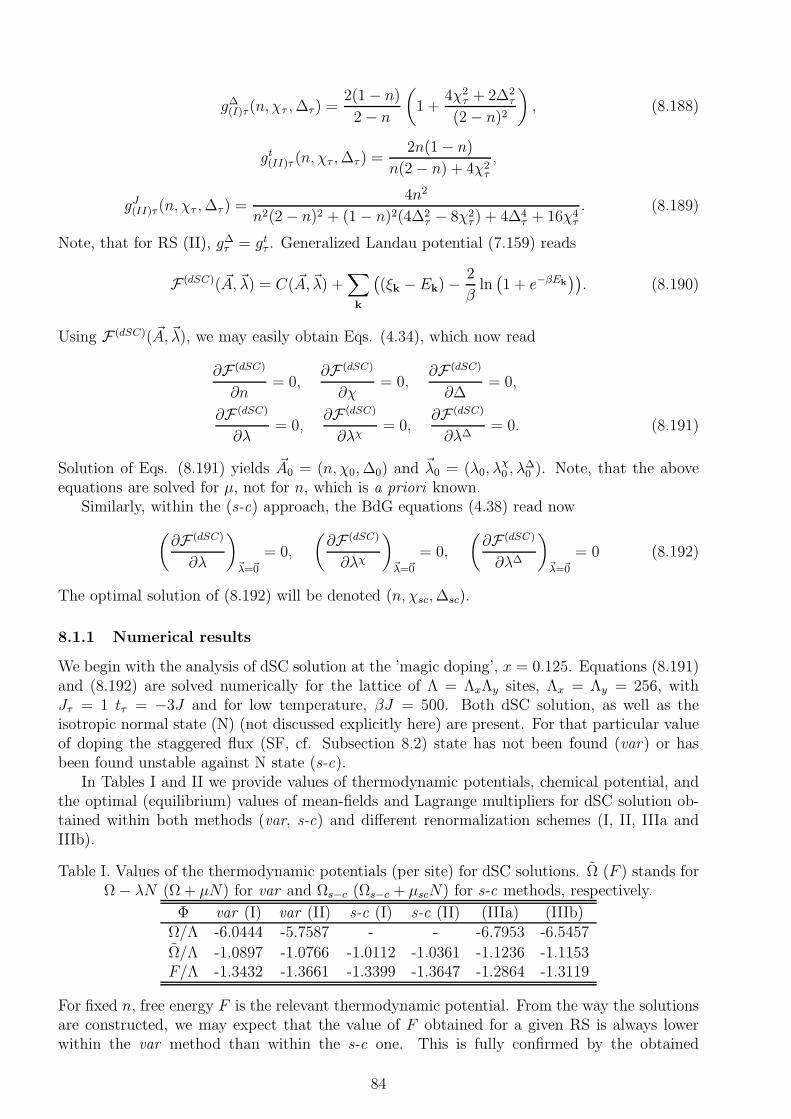
g∆(I)τ (n, χτ ,∆τ ) =
2(1 − n)
2 − n
(
1 +4χ2
τ + 2∆2τ
(2 − n)2
)
, (8.188)
gt(II)τ (n, χτ ,∆τ ) =
2n(1 − n)
n(2 − n) + 4χ2τ
,
gJ(II)τ (n, χτ ,∆τ ) =
4n2
n2(2 − n)2 + (1 − n)2(4∆2τ − 8χ2
τ ) + 4∆4τ + 16χ4
τ
. (8.189)
Note, that for RS (II), g∆τ = gt
τ . Generalized Landau potential (7.159) reads
F (dSC)( ~A,~λ) = C( ~A,~λ) +∑
k
(
(ξk −Ek) − 2
βln(
1 + e−βEk))
. (8.190)
Using F (dSC)( ~A,~λ), we may easily obtain Eqs. (4.34), which now read
∂F (dSC)
∂n= 0,
∂F (dSC)
∂χ= 0,
∂F (dSC)
∂∆= 0,
∂F (dSC)
∂λ= 0,
∂F (dSC)
∂λχ= 0,
∂F (dSC)
∂λ∆= 0. (8.191)
Solution of Eqs. (8.191) yields ~A0 = (n, χ0,∆0) and ~λ0 = (λ0, λχ0 , λ
∆0 ). Note, that the above
equations are solved for µ, not for n, which is a priori known.Similarly, within the (s-c) approach, the BdG equations (4.38) read now
(
∂F (dSC)
∂λ
)
~λ=~0
= 0,
(
∂F (dSC)
∂λχ
)
~λ=~0
= 0,
(
∂F (dSC)
∂λ∆
)
~λ=~0
= 0 (8.192)
The optimal solution of (8.192) will be denoted (n, χsc,∆sc).
8.1.1 Numerical results
We begin with the analysis of dSC solution at the ’magic doping’, x = 0.125. Equations (8.191)and (8.192) are solved numerically for the lattice of Λ = ΛxΛy sites, Λx = Λy = 256, withJτ = 1 tτ = −3J and for low temperature, βJ = 500. Both dSC solution, as well as theisotropic normal state (N) (not discussed explicitly here) are present. For that particular valueof doping the staggered flux (SF, cf. Subsection 8.2) state has not been found (var) or hasbeen found unstable against N state (s-c).
In Tables I and II we provide values of thermodynamic potentials, chemical potential, andthe optimal (equilibrium) values of mean-fields and Lagrange multipliers for dSC solution ob-tained within both methods (var, s-c) and different renormalization schemes (I, II, IIIa andIIIb).
Table I. Values of the thermodynamic potentials (per site) for dSC solutions. Ω (F ) stands forΩ − λN (Ω + µN) for var and Ωs−c (Ωs−c + µscN) for s-c methods, respectively.
Φ var (I) var (II) s-c (I) s-c (II) (IIIa) (IIIb)Ω/Λ -6.0444 -5.7587 - - -6.7953 -6.5457
Ω/Λ -1.0897 -1.0766 -1.0112 -1.0361 -1.1236 -1.1153F/Λ -1.3432 -1.3661 -1.3399 -1.3647 -1.2864 -1.3119
For fixed n, free energy F is the relevant thermodynamic potential. From the way the solutionsare constructed, we may expect that the value of F obtained for a given RS is always lowerwithin the var method than within the s-c one. This is fully confirmed by the obtained
84
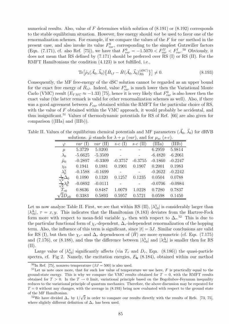
numerical results. Also, value of F determines which solution of (8.191) or (8.192) correspondsto the stable equilibrium situation. However, free energy should not be used to favor one of therenormalization schemes. For example, if we compare the values of the F for var method in thepresent case, and also invoke its value F 0
var , corresponding to the simplest Gutzwiller factors(Eqn. (7.171), cf. also Ref. [75]), we have that F 0
var = −1.5070 < F IIvar < F I
var .50 Obviously, itdoes not mean that RS defined by (7.171) should be preferred over RS (I) or RS (II). For theRMFT Hamiltonians the condition (4.123) is not fulfilled, i.e.,
Tr[
ρλ( ~A0, ~λ0)
HtJ − H( ~A0, ~λ0)(dSC)Rλ
]
6= 0. (8.193)
Consequently, the MF free-energy of the dSC solution cannot be regarded as an upper boundfor the exact free energy of HtJ . Indeed, value F 0
var is much lower then the Variational MonteCarlo (VMC) result (EV MC ≈ −1.33) [75], hence it is very likely that F 0
var is also lower then theexact value (the latter remark is valid for other renormalization schemes as well). Also, if therewas a good agreement between Fvar obtained within the RMFT for the particular choice of RS,with the value of F obtained within the VMC approach, it would probably be accidental, andthus insignificant.51 Values of thermodynamic potentials for RS of Ref. [66] are also given forcomparison ((IIIa) and (IIIb)).
Table II. Values of the equilibrium chemical potentials and MF parameters ( ~A0, ~λ0) for dRVBsolutions. µ stands for λ+ µ (var), and for µsc (s-c).
ϕ var (I) var (II) s-c (I) s-c (II) (IIIa) (IIIb)µ 5.3729 5.0200 - - 6.2959 5.9814λ0 -5.6625 -5.3509 - - -6.4820 -6.2061µ0 -0.2897 -0.3309 -0.3757 -0.3755 -0.1860 -0.2247χ0 0.1941 0.1881 0.1901 0.1907 0.2001 0.1983λχ
0 -0.1588 -0.1699 - - -0.2622 -0.22421√2∆0 0.1090 0.1320 0.1257 0.1235 0.0504 0.0788
1√2λ∆
0 -0.0892 -0.0111 - - -0.0706 -0.0984
Tτ0 0.8636 0.8487 1.0079 1.0228 0.7280 0.7837√2Dx0 0.3383 0.5893 0.5957 0.5721 0.0598 0.1450
Let us now analyze Table II. First, we see that within RS (II), |λχτ0| is considerably larger than
|λ∆τ0|, τ = x, y. This indicates that the Hamiltonian (8.183) deviates from the Hartree-Fock
form more with respect to mean-field variable χτ then with respect to ∆τ .52 This is due tothe particular functional form of χτ -dependent, ∆τ -independent renormalization of the hoppingterm. Also, the influence of this term is significant, since |t| = 3J . Similar conclusions are validfor RS (I), but then the χτ - and ∆τ dependences of 〈H〉 are more symmetric (cf. Eqs. (7.175)and (7.176), or (8.188), and thus the difference between |λχ
τ0| and |λ∆τ0| is smaller then for RS
(II).Large value of |λχ
τ0| significantly affects (via Tτ and Dτ , Eqn. (8.186)) the quasi-particlespectra, cf. Fig 2. Namely, the excitation energies, Ek (8.184), obtained within our method
50In Ref. [75], nonzero temperature (βJ = 500) is also used.51Let us note once more, that for such low value of temperature we use here, F is practically equal to the
ground-state energy. This is why we compare the VMC results obtained for T = 0, with the RMFT resultsobtained for T > 0. In the T → 0 limit, variational principle based on the Bogoliubov-Feynman inequalityreduces to the variational principle of quantum mechanics. Therefore, the above discussion may be repeated forT = 0 without any changes, with the average in (8.193) being now evaluated with respect to the ground stateof the MF Hamiltonian.
52We have divided ∆τ by 1/√
2 in order to compare our results directly with the results of Refs. [73, 75],where slightly different definition of ∆τ has been used.
85
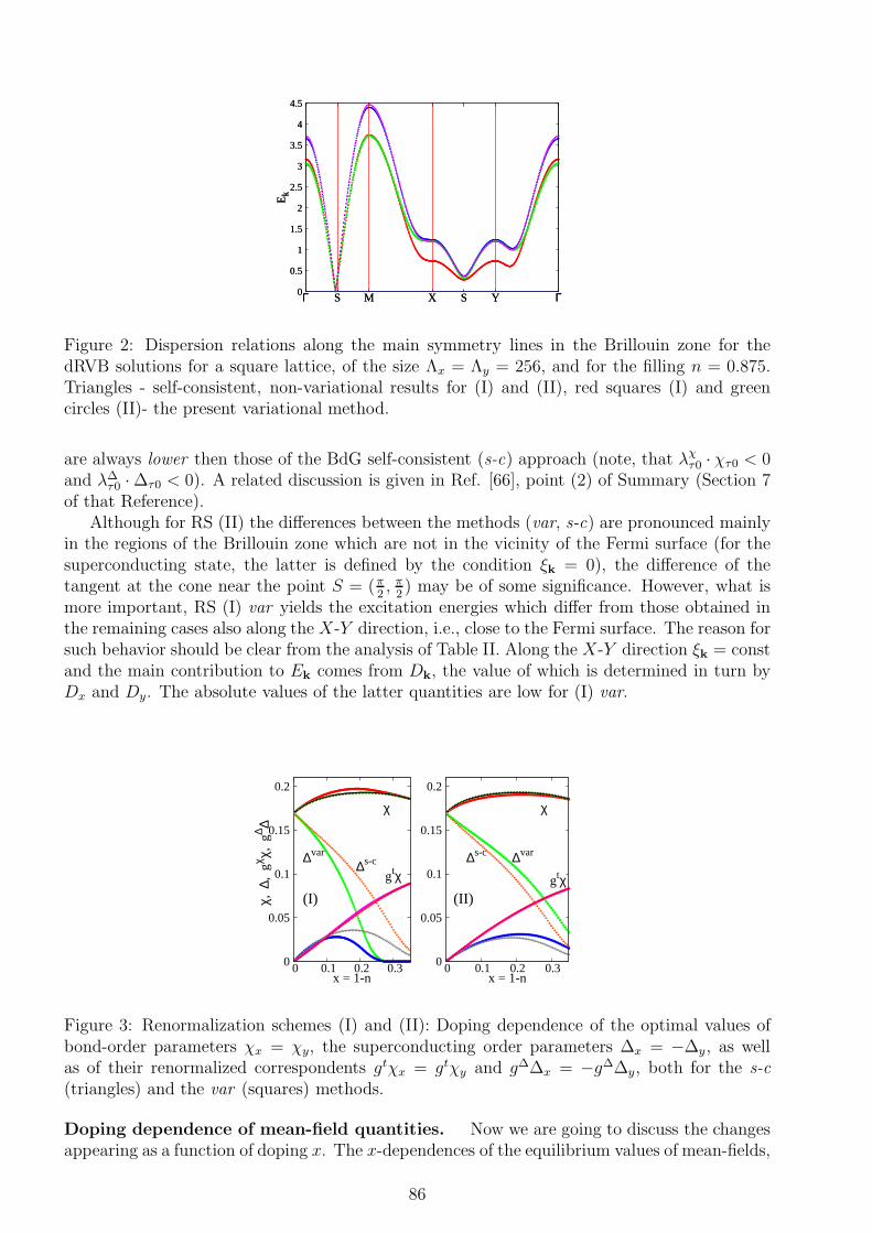
0
0.5
1
1.5
2
2.5
3
3.5
4
4.5
Γ S M X S Y ΓE
k 0
0.5
1
1.5
2
2.5
3
3.5
4
4.5
Γ S M X S Y ΓE
k
Figure 2: Dispersion relations along the main symmetry lines in the Brillouin zone for thedRVB solutions for a square lattice, of the size Λx = Λy = 256, and for the filling n = 0.875.Triangles - self-consistent, non-variational results for (I) and (II), red squares (I) and greencircles (II)- the present variational method.
are always lower then those of the BdG self-consistent (s-c) approach (note, that λχτ0 · χτ0 < 0
and λ∆τ0 · ∆τ0 < 0). A related discussion is given in Ref. [66], point (2) of Summary (Section 7
of that Reference).Although for RS (II) the differences between the methods (var, s-c) are pronounced mainly
in the regions of the Brillouin zone which are not in the vicinity of the Fermi surface (for thesuperconducting state, the latter is defined by the condition ξk = 0), the difference of thetangent at the cone near the point S = (π
2, π
2) may be of some significance. However, what is
more important, RS (I) var yields the excitation energies which differ from those obtained inthe remaining cases also along the X-Y direction, i.e., close to the Fermi surface. The reason forsuch behavior should be clear from the analysis of Table II. Along the X-Y direction ξk = constand the main contribution to Ek comes from Dk, the value of which is determined in turn byDx and Dy. The absolute values of the latter quantities are low for (I) var.
0
0.05
0.1
0.15
0.2
0 0.1 0.2 0.3
χ
, ∆,
gχ χ,
g∆ ∆
x = 1-n
gtχ
χ
∆var
∆s-c
(I)
0
0.05
0.1
0.15
0.2
0 0.1 0.2 0.3x = 1-n
χ
∆s-c ∆var
(II)gtχ
Figure 3: Renormalization schemes (I) and (II): Doping dependence of the optimal values ofbond-order parameters χx = χy, the superconducting order parameters ∆x = −∆y , as wellas of their renormalized correspondents gtχx = gtχy and g∆∆x = −g∆∆y, both for the s-c
(triangles) and the var (squares) methods.
Doping dependence of mean-field quantities. Now we are going to discuss the changesappearing as a function of doping x. The x-dependences of the equilibrium values of mean-fields,
86
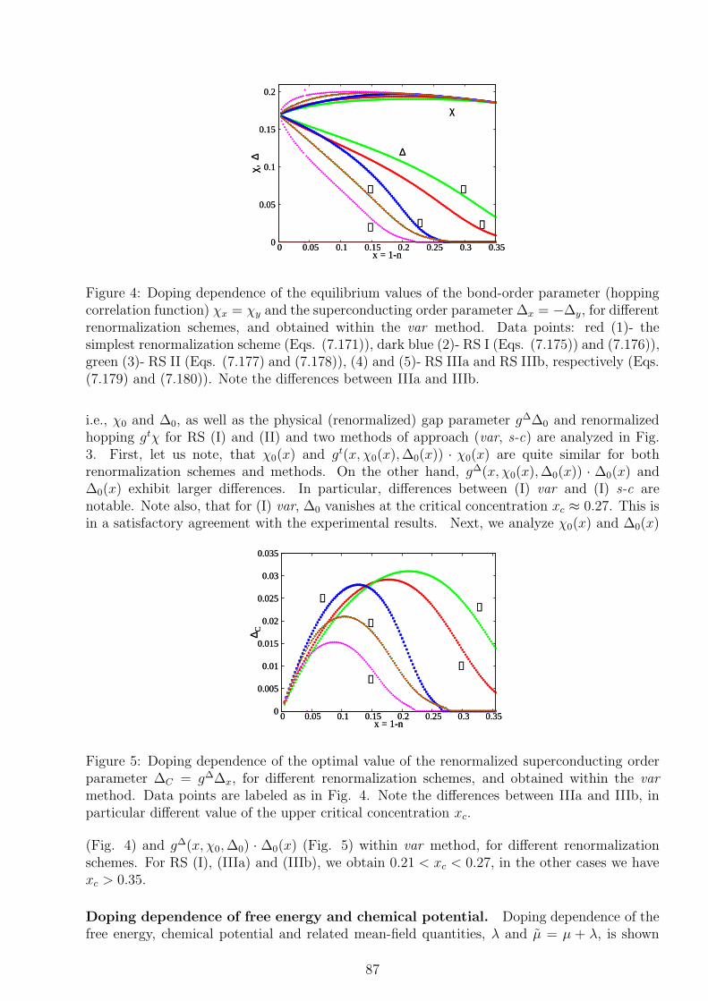
0
0.05
0.1
0.15
0.2
0 0.05 0.1 0.15 0.2 0.25 0.3 0.35χ,
∆x = 1-n
➌
➊➋➍
➎
χ
∆
0
0.05
0.1
0.15
0.2
0 0.05 0.1 0.15 0.2 0.25 0.3 0.35χ,
∆x = 1-n
➌
➊➋➍
➎
χ
∆
Figure 4: Doping dependence of the equilibrium values of the bond-order parameter (hoppingcorrelation function) χx = χy and the superconducting order parameter ∆x = −∆y, for differentrenormalization schemes, and obtained within the var method. Data points: red (1)- thesimplest renormalization scheme (Eqs. (7.171)), dark blue (2)- RS I (Eqs. (7.175)) and (7.176)),green (3)- RS II (Eqs. (7.177) and (7.178)), (4) and (5)- RS IIIa and RS IIIb, respectively (Eqs.(7.179) and (7.180)). Note the differences between IIIa and IIIb.
i.e., χ0 and ∆0, as well as the physical (renormalized) gap parameter g∆∆0 and renormalizedhopping gtχ for RS (I) and (II) and two methods of approach (var, s-c) are analyzed in Fig.3. First, let us note, that χ0(x) and gt(x, χ0(x),∆0(x)) · χ0(x) are quite similar for bothrenormalization schemes and methods. On the other hand, g∆(x, χ0(x),∆0(x)) · ∆0(x) and∆0(x) exhibit larger differences. In particular, differences between (I) var and (I) s-c arenotable. Note also, that for (I) var, ∆0 vanishes at the critical concentration xc ≈ 0.27. This isin a satisfactory agreement with the experimental results. Next, we analyze χ0(x) and ∆0(x)
0
0.005
0.01
0.015
0.02
0.025
0.03
0.035
0 0.05 0.1 0.15 0.2 0.25 0.3 0.35
∆ C
x = 1-n
➊
➌➋
➎
➍
0
0.005
0.01
0.015
0.02
0.025
0.03
0.035
0 0.05 0.1 0.15 0.2 0.25 0.3 0.35
∆ C
x = 1-n
➊
➌➋
➎
➍
Figure 5: Doping dependence of the optimal value of the renormalized superconducting orderparameter ∆C = g∆∆x, for different renormalization schemes, and obtained within the var
method. Data points are labeled as in Fig. 4. Note the differences between IIIa and IIIb, inparticular different value of the upper critical concentration xc.
(Fig. 4) and g∆(x, χ0,∆0) · ∆0(x) (Fig. 5) within var method, for different renormalizationschemes. For RS (I), (IIIa) and (IIIb), we obtain 0.21 < xc < 0.27, in the other cases we havexc > 0.35.
Doping dependence of free energy and chemical potential. Doping dependence of thefree energy, chemical potential and related mean-field quantities, λ and µ = µ + λ, is shown
87

-6
-4
-2
0
2
4
6
0 0.05 0.1 0.15 0.2 0.25 0.3 0.351-n = x
µ
Fvar, Fs-c
λ + µ, µs-c
λ
Figure 6: RS II: Doping dependences of the free energy (Fvar, Fs−c), the chemical potentials µ,µsc as well as that of λ and µ = λ+µ for the dSC state, obtained both within the present (var)and the (s-c) methods.
in Fig. 6, but only for RS (II). We emphasize once again, the chemical potential µ is the firstderivative of F/Λ with respect to n, unlike in some of the previous mean-fields treatments[63, 68, 73, 75]. Note that neither µ nor λ have this property, as discussed in Subsection4.7. Therefore, application of the standard thermodynamic identities and methods (e.g. theMaxwell construction) is probably not legitimate within such an approach, although this factis sometimes ignored (cf. [78]).
8.2 Staggered flux solution
As a next example we analyze the staggered-flux (SF) state, first proposed by Affleck andMarston [114] as a variational trial MF state for the Heisenberg model on the square lattice.Later, the SF state has been investigated in a number of papers (cf. e.g. [62, 115, 116, 117, 118,119, 120, 121, 122, 123, 124, 194]), also because this state has been proposed as a candidate forthe pseudogap phase in the cuprates [118]. SF state is also known to be one of most competitive(i.e., of lowest energy) states among the non-superconducting, non-magnetic ground states ofthe MF Hamiltonian (7.153) for a wide range of the values of its parameters [75]. Moreover,a state in which superconducting and SF orders coexist, has even lower energy [51]. Also,for n = 1, as a consequence of the local SU(2) symmetry, SF state is equivalent to the RVBstate of dx2−y2 symmetry (as well as to many other MF states, e.g. s + id wave state), [8, 58].Therefore, even if SF state is not a superconducting state, it is very interesting in the contextof the physics of cuprates, and deserves at least a brief analysis. However, here we are goingto use SF state mainly as yet another convenient example, on which the differences betweenvariational (var) and non-variational (s-c) solutions can be shown. We concentrate on RS (I)and (II), which, in the absence of superconducting order have quite similar form, and thereforethe modifications caused by a method of solution (var, s-c) become dominant.
The SF state differs from the simplest Fermi sea (N) state by a presence of the complexhopping amplitude between the nearest neighboring sites
χij = |χ| exp((−1)(ix+jy)iϕ) ≡ ξ1 ± iξ2. (8.194)
Complex χij imply the existence of circulating currents, direction of which changes from oneelementary plaquette53 to another in an alternating fashion. Consequently, a two-sublattice
53By an elementary plaquette we understand a square made of four sites (equivalently, bonds), which side isequal one lattice constant.
88

structure (’orbital antiferromagnet’ [62]) emerges, with the unit cell of the size√
2a×√
2a (ais a lattice constant) in direct space and new folded Brillouin zone (NBZ).
Solving this problem within the framework of our method, we have to add appropriateconstraints to the MF Hamiltonian according to Eq (7.157). This step introduces, apart fromthe molecular field λ coupled to n, also a complex Lagrange multiplier ηij = η1∓ iη2, connectedto χij (our sign convention for imaginary part of ηij for each bond is opposite to that for χij).
Thus, we have three independent real mean fields ~A = (n, ξ1, ξ2), and three corresponding real
Lagrange multipliers, ~λ = (λ, η1, η2). In the present case the renormalization factors (7.176)and (7.178) read, respectively
gt(I)(n, ξ1, ξ2) =
2(1 − n)
2 − n
(
1 − 4 (ξ21 + ξ2
2)
(2 − n)2
)
, gJ(I)(n, ξ1, ξ2) =
4
(2 − n)2. (8.195)
gt(II)(n, ξ1, ξ2) =
2n(1 − n)
n(2 − n) + 4(ξ21 + ξ2
2),
gJ(II)(n, ξ1, ξ2) =
4n2
n2(2 − n)2 − 8(1 − n)2(ξ21 + ξ2
2) + 16(ξ21 + ξ2
2)2. (8.196)
Diagonalization of HRλ (7.157) (in the present case denoted as H(SF )Rλ ), yields
H(SF )Rλ ( ~A,~λ) − µN = C( ~A,~λ) +
NBZ∑
ksσ
Eksσα†ksσαksσ, (8.197)
where Eksσ = −µ + s√
ǫ2k + χ2k, ǫk = T1Γ+(k), χk = T2Γ−(k), µ ≡ µ + λ, and for each k,
s = ±1 labels two sub-bands (two eigenvalues of the 2 × 2 matrix resulting from the Fouriertransform. Operator α†
ksσ (αksσ) creates (annihilates) quasiparticle with the quasimomentumk, spin σ and the band index s. Also, Γ±(k) ≡ 2(cos(kx) ± cos(ky)), and
T1 = tgt +3
4JgJξ1 + η1, T2 =
3
4JgJξ2 + η2, (8.198)
C( ~A,~λ) = Λ(
λn + 3gJ(ξ21 + ξ2
2) + 8(ξ1η1 + ξ2η2))
. (8.199)
Generalized Landau potential (7.159) takes now the following form
F (SF )( ~A,~λ) = C( ~A,~λ) − 1
β
NBZ∑
ksσ
ln(
1 + e−βEksσ
)
. (8.200)
Using F (SF )( ~A,~λ), we obtain Eqs. (4.34), which now read
∂F (SF )
∂n= 0,
∂F (SF )
∂ξ1= 0,
∂F (SF )
∂ξ2= 0,
∂F (SF )
∂λ= 0,
∂F (SF )
∂η1= 0,
∂F (SF )
∂η2= 0. (8.201)
Explicit form of the above equations will not be provided here. Solving Eqs. (8.201), we obtain~A0 ≡ (n, ξ
(0)1 , ξ
(0)2 ) and ~λ0 = (λ0, η
(0)1 , η
(0)2 ). As usual, for a given n the value of the chemical
potential µ is obtained from Eqs. (8.201).Similarity, within the (s-c) approach, we have to solve the following BdG equations (4.38)
(
∂F (SF )
∂λ
)
~λ=~0
= 0,
(
∂F (SF )
∂η1
)
~λ=~0
= 0,
(
∂F (SF )
∂η2
)
~λ=~0
= 0. (8.202)
Solution of (8.202) will be denoted ~Asc ≡ (n, ξ(sc)1 , ξ
(sc)2 ).
89
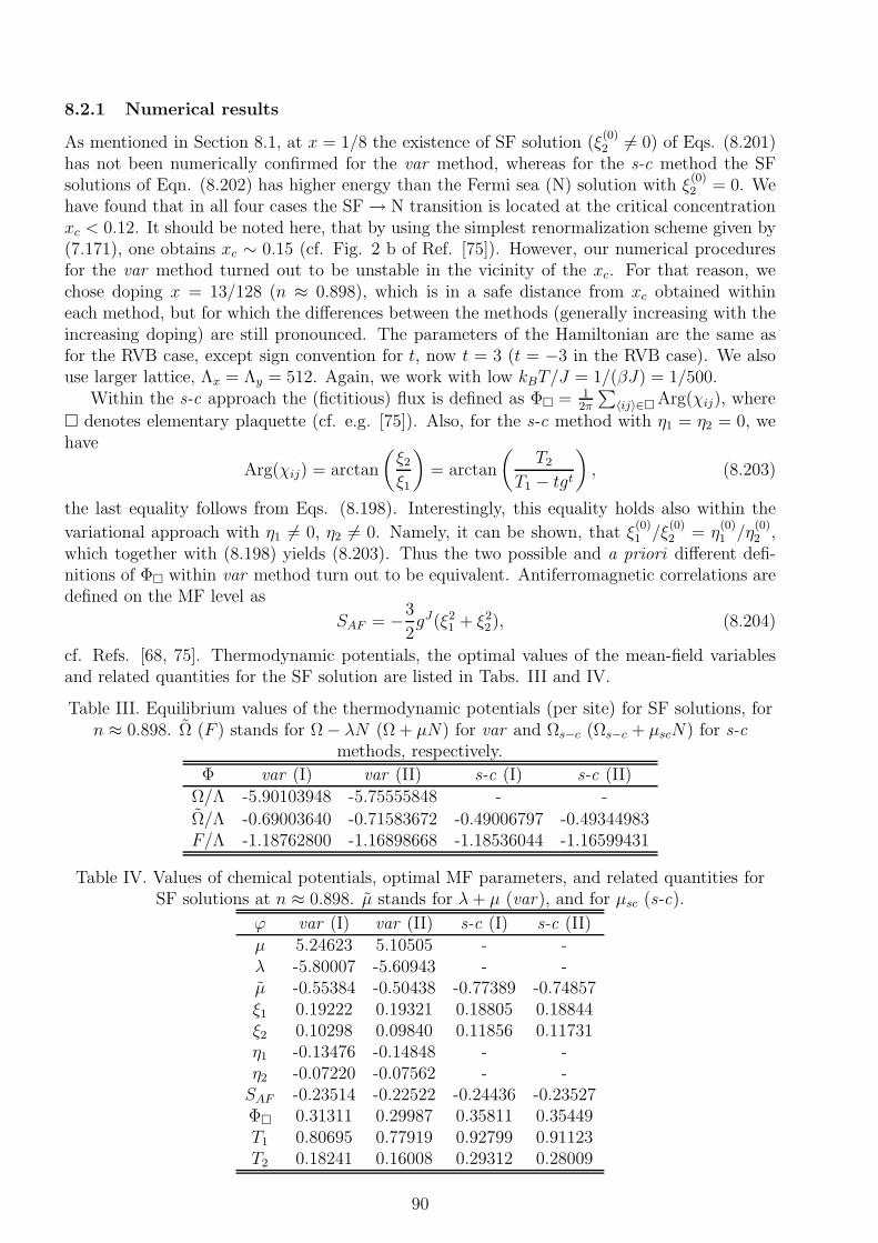
8.2.1 Numerical results
As mentioned in Section 8.1, at x = 1/8 the existence of SF solution (ξ(0)2 6= 0) of Eqs. (8.201)
has not been numerically confirmed for the var method, whereas for the s-c method the SFsolutions of Eqn. (8.202) has higher energy than the Fermi sea (N) solution with ξ
(0)2 = 0. We
have found that in all four cases the SF → N transition is located at the critical concentrationxc < 0.12. It should be noted here, that by using the simplest renormalization scheme given by(7.171), one obtains xc ∼ 0.15 (cf. Fig. 2 b of Ref. [75]). However, our numerical proceduresfor the var method turned out to be unstable in the vicinity of the xc. For that reason, wechose doping x = 13/128 (n ≈ 0.898), which is in a safe distance from xc obtained withineach method, but for which the differences between the methods (generally increasing with theincreasing doping) are still pronounced. The parameters of the Hamiltonian are the same asfor the RVB case, except sign convention for t, now t = 3 (t = −3 in the RVB case). We alsouse larger lattice, Λx = Λy = 512. Again, we work with low kBT/J = 1/(βJ) = 1/500.
Within the s-c approach the (fictitious) flux is defined as Φ = 12π
∑
〈ij〉∈Arg(χij), where
denotes elementary plaquette (cf. e.g. [75]). Also, for the s-c method with η1 = η2 = 0, wehave
Arg(χij) = arctan
(
ξ2ξ1
)
= arctan
(
T2
T1 − tgt
)
, (8.203)
the last equality follows from Eqs. (8.198). Interestingly, this equality holds also within the
variational approach with η1 6= 0, η2 6= 0. Namely, it can be shown, that ξ(0)1 /ξ
(0)2 = η
(0)1 /η
(0)2 ,
which together with (8.198) yields (8.203). Thus the two possible and a priori different defi-nitions of Φ within var method turn out to be equivalent. Antiferromagnetic correlations aredefined on the MF level as
SAF = −3
2gJ(ξ2
1 + ξ22), (8.204)
cf. Refs. [68, 75]. Thermodynamic potentials, the optimal values of the mean-field variablesand related quantities for the SF solution are listed in Tabs. III and IV.
Table III. Equilibrium values of the thermodynamic potentials (per site) for SF solutions, forn ≈ 0.898. Ω (F ) stands for Ω − λN (Ω + µN) for var and Ωs−c (Ωs−c + µscN) for s-c
methods, respectively.
Φ var (I) var (II) s-c (I) s-c (II)Ω/Λ -5.90103948 -5.75555848 - -
Ω/Λ -0.69003640 -0.71583672 -0.49006797 -0.49344983F/Λ -1.18762800 -1.16898668 -1.18536044 -1.16599431
Table IV. Values of chemical potentials, optimal MF parameters, and related quantities forSF solutions at n ≈ 0.898. µ stands for λ+ µ (var), and for µsc (s-c).
ϕ var (I) var (II) s-c (I) s-c (II)µ 5.24623 5.10505 - -λ -5.80007 -5.60943 - -µ -0.55384 -0.50438 -0.77389 -0.74857ξ1 0.19222 0.19321 0.18805 0.18844ξ2 0.10298 0.09840 0.11856 0.11731η1 -0.13476 -0.14848 - -η2 -0.07220 -0.07562 - -SAF -0.23514 -0.22522 -0.24436 -0.23527Φ 0.31311 0.29987 0.35811 0.35449T1 0.80695 0.77919 0.92799 0.91123T2 0.18241 0.16008 0.29312 0.28009
90
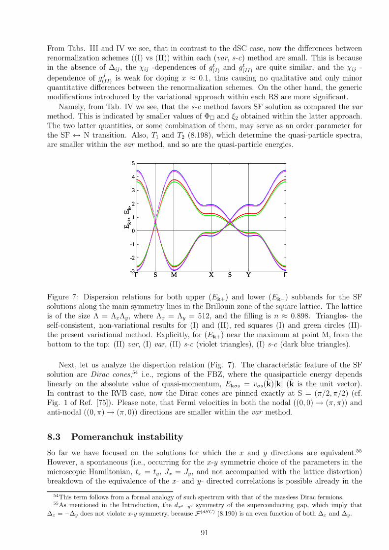
From Tabs. III and IV we see, that in contrast to the dSC case, now the differences betweenrenormalization schemes ((I) vs (II)) within each (var, s-c) method are small. This is becausein the absence of ∆ij , the χij -dependences of gt
(I) and gt(II) are quite similar, and the χij -
dependence of gJ(II) is weak for doping x ≈ 0.1, thus causing no qualitative and only minor
quantitative differences between the renormalization schemes. On the other hand, the genericmodifications introduced by the variational approach within each RS are more significant.
Namely, from Tab. IV we see, that the s-c method favors SF solution as compared the var
method. This is indicated by smaller values of Φ and ξ2 obtained within the latter approach.The two latter quantities, or some combination of them, may serve as an order parameter forthe SF ↔ N transition. Also, T1 and T2 (8.198), which determine the quasi-particle spectra,are smaller within the var method, and so are the quasi-particle energies.
-3
-2
-1
0
1
2
3
4
5
Γ S M X S Y Γ
Ek+
, E
k-
-3
-2
-1
0
1
2
3
4
5
Γ S M X S Y Γ
Ek+
, E
k-
Figure 7: Dispersion relations for both upper (Ek+) and lower (Ek−) subbands for the SFsolutions along the main symmetry lines in the Brillouin zone of the square lattice. The latticeis of the size Λ = ΛxΛy, where Λx = Λy = 512, and the filling is n ≈ 0.898. Triangles- theself-consistent, non-variational results for (I) and (II), red squares (I) and green circles (II)-the present variational method. Explicitly, for (Ek+) near the maximum at point M, from thebottom to the top: (II) var, (I) var, (II) s-c (violet triangles), (I) s-c (dark blue triangles).
Next, let us analyze the dispertion relation (Fig. 7). The characteristic feature of the SFsolution are Dirac cones,54 i.e., regions of the FBZ, where the quasiparticle energy dependslinearly on the absolute value of quasi-momentum, Ekσs = vσs(k)|k| (k is the unit vector).In contrast to the RVB case, now the Dirac cones are pinned exactly at S = (π/2, π/2) (cf.Fig. 1 of Ref. [75]). Please note, that Fermi velocities in both the nodal ((0, 0) → (π, π)) andanti-nodal ((0, π) → (π, 0)) directions are smaller within the var method.
8.3 Pomeranchuk instability
So far we have focused on the solutions for which the x and y directions are equivalent.55
However, a spontaneous (i.e., occurring for the x-y symmetric choice of the parameters in themicroscopic Hamiltonian, tx = ty, Jx = Jy, and not accompanied with the lattice distortion)breakdown of the equivalence of the x- and y- directed correlations is possible already in the
54This term follows from a formal analogy of such spectrum with that of the massless Dirac fermions.55As mentioned in the Introduction, the dx2−y2 symmetry of the superconducting gap, which imply that
∆x = −∆y does not violate x-y symmetry, because F (dSC) (8.190) is an even function of both ∆x and ∆y.
91
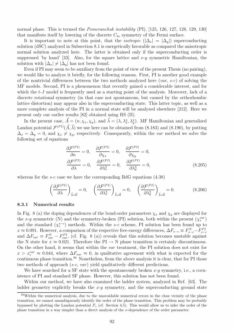
normal phase. This is termed the Pomeranchuk instability (PI), [125, 126, 127, 128, 129, 130]that manifests itself by lowering of the discrete C4v symmetry of the Fermi surface.
It is important to note at this point, that the isotropic (|∆x| = |∆y|) superconductingsolution (dSC) analyzed in Subsection 8.1 is energetically favorable as compared the anisotropicnormal solution analyzed here. The latter is obtained only if the superconducting order issuppressed ’by hand’ [33]. Also, for the square lattice and x-y symmetric Hamiltonian, thesolution with |∆x| 6= |∆y| has not been found.
Even if PI may seem to be auxiliary from the point of view of the present Thesis (no pairing),we would like to analyze it briefly, for the following reasons. First, PI is another good exampleof the nontrivial differences between the two methods analyzed here (var, s-c) of solving theMF models. Second, PI is a phenomenon that recently gained a considerable interest, and forwhich the t-J model is frequently used as a starting point of the analysis. Moreover, lack of adiscrete rotational symmetry (in that case not spontaneous, but caused by the orthorhombiclattice distortion) may appear also in the superconducting state. This latter topic, as well as amore complete analysis of the PI in a normal state will be analyzed elsewhere [212]. Here wepresent only our earlier results [82] obtained using RS (II).
In the present case, ~A = (n, χx, χy), and ~λ = (λ, λχx, λ
χy ). MF Hamiltonian and generalized
Landau potential F (PI)( ~A,~λ) we use here can be obtained from (8.183) and (8.190), by putting∆x = ∆y = 0, and χx 6= χy, respectively. Consequently, within the var method we solve thefollowing set of equations
∂F (PI)
∂n= 0,
∂F (PI)
∂χx= 0,
∂F (PI)
∂χy= 0,
∂F (PI)
∂λ= 0,
∂F (PI)
∂λχx
= 0,∂F (PI)
∂λχy
= 0, (8.205)
whereas for the s-c case we have the corresponding BdG equations (4.38)
(
∂F (PI)
∂λ
)
~λ=~0
= 0,
(
∂F (PI)
∂λχx
)
~λ=~0
= 0,
(
∂F (PI)
∂λχy
)
~λ=~0
= 0. (8.206)
8.3.1 Numerical results
In Fig. 8 (a) the doping dependences of the bond-order parameters χx and χy are displayed forthe x-y symmetric (N) and the symmetry-broken (PI) solution, both within the present (χvar
τ )and the standard (χs−c
τ ) methods. Within the s-c scheme, PI solution has been found up tox ≈ 0.091. However, a comparison of the respective free-energy differences, ∆Fs−c ≡ FN
s−c−F PIs−c
and ∆Fvar ≡ FNvar − F PI
var , (cf. Fig. 8 (a)) reveals that this solution becomes unstable againstthe N state for x ≈ 0.021. Therefore the PI → N phase transition is certainly discontinuous.On the other hand, it seems that within the var treatment, the PI solution does not exist forx > xvar
c ≈ 0.044, where ∆Fvar ≈ 0, in qualitative agreement with what is expected for thecontinuous phase transition.56 Nonetheless, from the above analysis it is clear, that for PI thosetwo methods of approach (s-c, var) yield qualitatively different predictions.
We have searched for a SF state with the spontaneously broken x-y symmetry, i.e., a coex-istence of PI and standard SF phase. However, this solution has not been found.
Within our method, we have also examined the ladder system, analyzed in Ref. [63]. Theladder geometry explicitly breaks the x-y symmetry, and the superconducting ground state
56Within the numerical analysis, due to the unavoidable numerical errors in the close vicinity of the phasetransition, we cannot unambiguously identify the order of the phase transition. This problem may be probablybypassed by plotting the Landau potential Fz (cf. Section 4.5). This would allow us to infer the order of thephase transition in a way simpler than a direct analysis of the x-dependence of the order parameter.
92
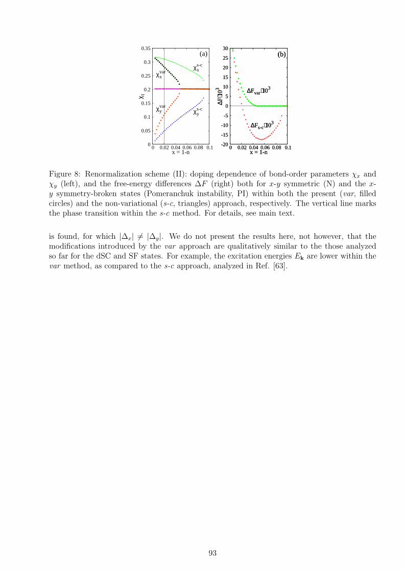
0
0.05
0.1
0.15
0.2
0.25
0.3
0.35
0 0.02 0.04 0.06 0.08 0.1
χ τ
x = 1-n
χxvar
χyvar
χxs-c
χys-c
(a)
-20
-15
-10
-5
0
5
10
15
20
25
30
0 0.02 0.04 0.06 0.08 0.1
∆F⋅1
03
x = 1-n
∆Fs-c⋅103
∆Fvar⋅103
(b)
-20
-15
-10
-5
0
5
10
15
20
25
30
0 0.02 0.04 0.06 0.08 0.1
∆F⋅1
03
x = 1-n
∆Fs-c⋅103
∆Fvar⋅103
(b)
Figure 8: Renormalization scheme (II): doping dependence of bond-order parameters χx andχy (left), and the free-energy differences ∆F (right) both for x-y symmetric (N) and the x-y symmetry-broken states (Pomeranchuk instability, PI) within both the present (var, filledcircles) and the non-variational (s-c, triangles) approach, respectively. The vertical line marksthe phase transition within the s-c method. For details, see main text.
is found, for which |∆x| 6= |∆y|. We do not present the results here, not however, that themodifications introduced by the var approach are qualitatively similar to the those analyzedso far for the dSC and SF states. For example, the excitation energies Ek are lower within thevar method, as compared to the s-c approach, analyzed in Ref. [63].
93
9 Results II: Optimal renormalization scheme and its
application to t-J model
In the previous Section, we have compared results obtained by using various renormalizationschemes (RS). Now, we apply the RS of Ref. [76] to study different forms of the t-J Hamiltonian(6.127). Also, the role of the next-nearest (t′) and next-next-nearest (t′′) neighbor hoppingintegrals is analyzed. The non-variational method based on the BdG equations (7.161) will nolonger be utilized. Consequently, it is convenient to apply an alternative formulation of RMFT,as given by Eqs. (7.167) - (7.170) (Section 7.4.3). This Section provides the principal resultsof this Thesis for the t-J model.
9.1 Non-standard formulation of RMFT approach
9.1.1 RMFT Hamiltonian
Our point of departure is the RMFT Hamiltonian (7.165)
H(∼)Rλ = −
∑
〈ij〉σ
(
ηijσ
(
c†iσcjσ − χijσ
)
+ H.c.)
−∑
iσ
λ(n)iσ
(
niσ − niσ
)
)
−∑
〈ij〉
(
γij
(
∆ij − ∆ij
)
+ H.c.)
+W (χijσ,∆ij , niσ).
In above, ∆ij is given by Eqs. (7.166). To obtain an explicit form of W (χijσ,∆ij, niσ) =
〈HtJ〉appC appearing in (7.164) and (7.165), we assume that the following mean fields and the
corresponding Lagrange multipliers may take non-zero values: χij = ξs and ηijσ = ηij ≡ ηs,
with s = 1, 3, 5 corresponding to sites with d(i, j) ≡ |~Ri− ~Rj | equal 1,√
2, and 2 (in units of the
lattice constant a), respectively; ∆ij = 〈∆ij〉 = ∆x(y), with ∆x(y) = ±∆ and γij = γx(y) = ±γ(dx2−y2 symmetry), both nonzero for d(i, j) = 1 and zero otherwise, as well as niσ = niσ = n/2
and λ(n)iσ = λ. Therefore, we have
~A = (ξ1, ξ3, ξ5,∆, n), ~λ = (η1, η3, η5, γ, λ). (9.207)
Then, W ( ~A) is obtained by applying formalism of Ref. [76] (for more details, please consultAppendix D (Subsection 11.4) and the original paper). Explicitly, we have
W ( ~A) = Wt +WJ +W3, (9.208)
where
Wt
Λ=
16(1 − n)
2 − n
t1ξ1
(
1 − 4(∆2 + ξ21)
(2 − n)2
)
+∑
s=3,5
tsysξs
(
1 − 4ξ2s
(2 − n)2
)
, (9.209)
WJ
Λ= −4J
(
3 (∆2 + ξ21) + c1(1 − n)2 (∆2 − ξ2
1)
(2 − n)2
)
− Jc1n2/2, (9.210)
94

and
W3
Λ= −32c2J
(1 − n)
(2 − n)3·(
1 − n2
4
)
ξ21 + (2 − n)ξ2
1ξ3 −nξ3
3
2
+ nξ3∆2 +1
2nξ3
(
1 − n
2
)2
−(
1 − n
2
)(
2 − n
2
)
∆2
− 16c2J(1 − n)
(2 − n)3·(
1 − n2
4
)
ξ21 + (2 − n)ξ2
1ξ5 −nξ3
5
2
+ nξ5∆2 +1
2nξ5
(
1 − n
2
)2
+(
1 − n
2
)(
2 − n
2
)
∆2
+ c2t3J(1 − n)
|t1|(
1 − n2
)3 ·
ξ1
(
8(
1 − n
2
)
(
ξ21 + ξ2
3
)
+ 4n(
∆2 − ξ21
)
)
+ 16(n
2+ 1)(
1 − n
2
)
ξ1ξ3 + 4n(
1 − n
2
)2
ξ1
(9.211)
In the above formulas, Λ is the number of lattice sites. Parameters y3 and y5 in Wt (9.209),equal 0 or 1, allow us to select the way in which the hopping integrals to the more distantneighbors are renormalized. All presented results are for y3 = y5 = 1, but we comment alsoon the situation with either y3 or y5 equal zero. The model parameters are J , t1 = t, t3 = t′
and t5 = t′′. Note, that in HtJ (6.127) we retain all terms of order of t2/U (∼ J) and tt′/U(∼ J ′ ≡ Jt3/|t1|), and neglect a smaller terms ∼ (t′)2/U (∼ J ′′ ≡ J(t3/t1)2). As a consequence,we obtain the following MF grand Hamiltonian
K(α)λ ≡ −
∑
〈ij〉s
∑
σ
∑
s
(
ηs
(
c†iσcjσ − ξs)
+ H.c.)
−∑
〈ij〉
(
γ(
∆ij − ∆τ
)
+ H.c.)
− µ∑
iσ
niσ
−∑
iσ
(λniσ
(
niσ − n/2)
)
+W (ξs,∆τ , n). (9.212)
Next, we diagonalize Kλ (7.165) via the Bogoliubov-Valatin transformation. This step yields
K(α)λ =
∑
k
Ek(γ†k0γk0 + γ†k1γk1) +∑
k
(ξk − Ek) + C(α)( ~A,~λ), (9.213)
with
C(α)( ~A,~λ) = W ( ~A,~λ) + Λ(8∑
s
ξsηs + 4∆γ + λn). (9.214)
Also, we have
Ek =√
ξ2k +D2
k, Dk = −γ2
Γ−(k),
ξk = − (η1Γ+(k) + η3Θ(k) + η5Γ5(k) + µ) , (9.215)
with
Γ±(k) = 2(cos(kx) ± cos(ky)), Θ(k) = 4 cos(kx) cos(ky),
Γ5(k) = 2(cos(2kx) + cos(2ky)), and µ = µ+ λ. (9.216)
95
9.1.2 Generalized Landau potential and equations (4.34)
Using K(α)λ , we obtain the grand-canonical density operator (7.170), i.e., ρλ = Z−1
λ exp(−βK(α)λ ).
Consequently, generalized Landau potential (4.33) has the form
F = F (α) ≡ C(α) +∑
k
(
(ξk − Ek) − 2
βln(
1 + e−βEk))
. (9.217)
Eqs. (4.34), i.e., the necessary conditions for F (α) to have a minimum subject to constraintsread now
∂wF (α) = ∂wC(α) = ~05, (9.218)
∂zF (α) = ~05, (9.219)
where w ∈ ξ1, ξ3, ξ5,∆, n and z ∈ η1, η3, η5, γ, λ. In contrast to the formulation usedin Section 8, equations (9.218) may be easily solved in an analytic fashion. However, so-lutions of the remaining Eqs. (9.219) must be determined numerically. The optimal val-
ues of mean fields and Lagrange multipliers will be denoted ~A0 = (ξ(0)1 , ξ
(0)3 , ξ
(0)5 ,∆(0), n) and
~λ0 = (η(0)1 , η
(0)3 , η
(0)5 , γ(0), λ(0)), respectively.
Note, that within the present formulation, the quasiparticle energies Ek (9.215) dependfunctionally only on the Lagrange multipliers. Nonetheless, the latter become explicitly knownfunctions of mean-fields after Eqs. (9.218) are solved.
9.1.3 Characteristics of the model: qualitative analysis
The analytical expression for W ( ~A) (9.208) allows us to make some qualitative predictionsconcerning the properties of our MF model before any numerical analysis is carried out. Thisis because at low T , the entropic part of the free energy is small, and therefore
F ≈ U = W ( ~A0) =⟨
K(α)( ~A0)⟩
+ µN. (9.220)
First, from (9.209) we expect a strong tendency to the superconductivity suppression for higherdoping, as SC order leads to the band energy decrease ∼ ∆2. On the other hand, in that regimethe renormalized band energy becomes predominant over the exchange part. In effect, thenormal state is favored over SC for x > xc with xc smaller than obtained within previous MFtreatments [33, 39, 58, 61]. Second, from (9.210) we infer, that the influence of the νiνj/4 termon WJ is small except for the largest doping; this is due to the presence of the (1−n)2 pre-factor(the other term ∼ n2 merely shifts the chemical potential). On the other hand, W3 (9.211) ismultiplied only by (1−n) = x pre-factor. Consequently, for higher x this term becomes ratherimportant. This is also due to the large number of distinct three-site terms present for a giveninitial site and spin direction (eight for d(i, j) =
√2, and four for d(i, j) = 2). Also, this part
of W is expected to suppress the SC order, as the term ∼ ∆2 in W3 contains a factor, which ispositive for reasonable values of other mean fields. Therefore, the energy gain of forming thesuperconducting state is lower if the H3 term is present.
9.2 Numerical results
After Eqs. (9.218) are solved analytically for Lagrange multipliers, we solve numerically theremaining Eqs. (9.219) for the mean fields. Again, we use periodic boundary conditions on thelattice of Λ = ΛxΛy = 5122 sites, to minimize finite size effects, and assume that kBT = 2·10−3J ,(practically equivalent to T = 0). Also, in the most cases we take the parameters |t|/J = 3(corresponding to U/|t| = 12 for the Hubbard model), t′/t = 0 or −0.25, and t′′ = 0 (t′′ 6= 0 is
96
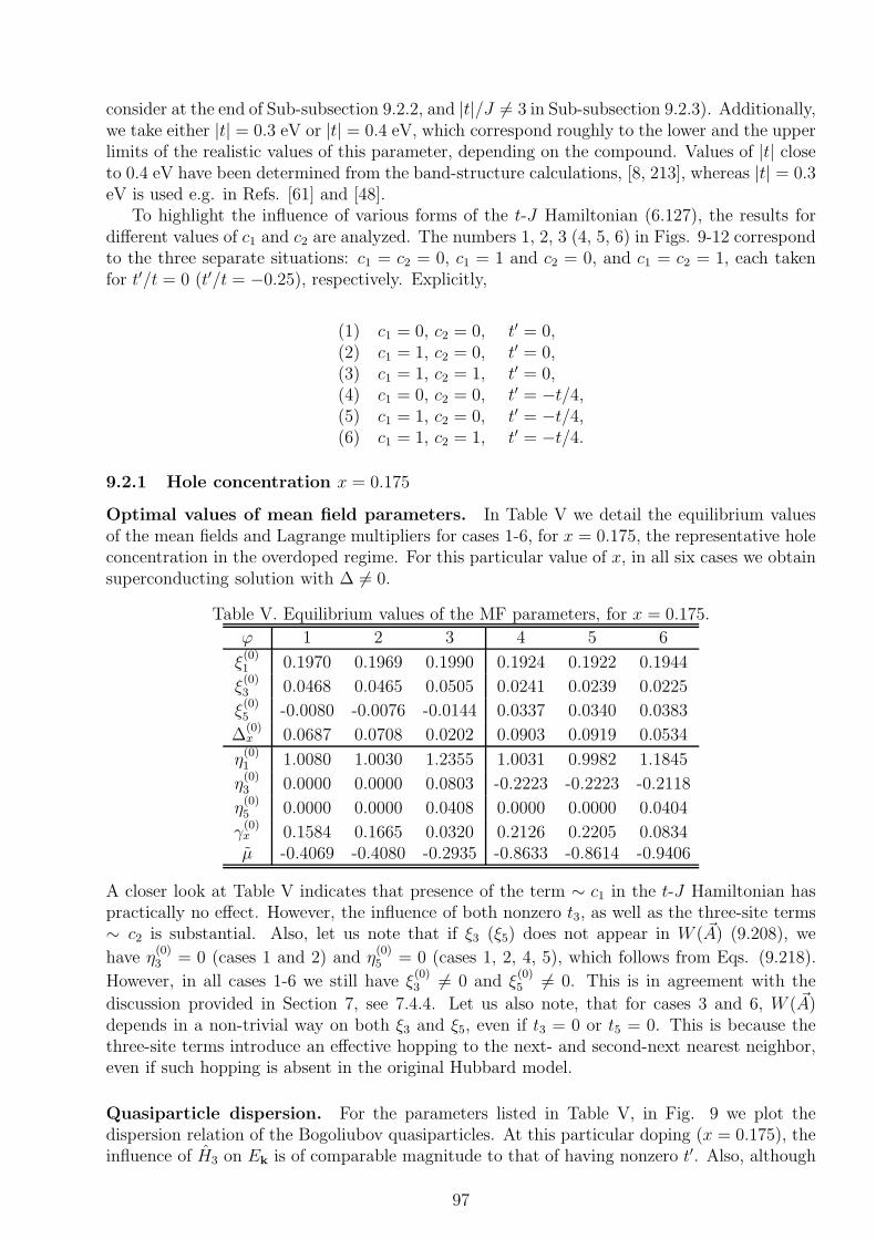
consider at the end of Sub-subsection 9.2.2, and |t|/J 6= 3 in Sub-subsection 9.2.3). Additionally,we take either |t| = 0.3 eV or |t| = 0.4 eV, which correspond roughly to the lower and the upperlimits of the realistic values of this parameter, depending on the compound. Values of |t| closeto 0.4 eV have been determined from the band-structure calculations, [8, 213], whereas |t| = 0.3eV is used e.g. in Refs. [61] and [48].
To highlight the influence of various forms of the t-J Hamiltonian (6.127), the results fordifferent values of c1 and c2 are analyzed. The numbers 1, 2, 3 (4, 5, 6) in Figs. 9-12 correspondto the three separate situations: c1 = c2 = 0, c1 = 1 and c2 = 0, and c1 = c2 = 1, each takenfor t′/t = 0 (t′/t = −0.25), respectively. Explicitly,
(1) c1 = 0, c2 = 0, t′ = 0,(2) c1 = 1, c2 = 0, t′ = 0,(3) c1 = 1, c2 = 1, t′ = 0,(4) c1 = 0, c2 = 0, t′ = −t/4,(5) c1 = 1, c2 = 0, t′ = −t/4,(6) c1 = 1, c2 = 1, t′ = −t/4.
9.2.1 Hole concentration x = 0.175
Optimal values of mean field parameters. In Table V we detail the equilibrium valuesof the mean fields and Lagrange multipliers for cases 1-6, for x = 0.175, the representative holeconcentration in the overdoped regime. For this particular value of x, in all six cases we obtainsuperconducting solution with ∆ 6= 0.
Table V. Equilibrium values of the MF parameters, for x = 0.175.
ϕ 1 2 3 4 5 6
ξ(0)1 0.1970 0.1969 0.1990 0.1924 0.1922 0.1944
ξ(0)3 0.0468 0.0465 0.0505 0.0241 0.0239 0.0225
ξ(0)5 -0.0080 -0.0076 -0.0144 0.0337 0.0340 0.0383
∆(0)x 0.0687 0.0708 0.0202 0.0903 0.0919 0.0534
η(0)1 1.0080 1.0030 1.2355 1.0031 0.9982 1.1845
η(0)3 0.0000 0.0000 0.0803 -0.2223 -0.2223 -0.2118
η(0)5 0.0000 0.0000 0.0408 0.0000 0.0000 0.0404
γ(0)x 0.1584 0.1665 0.0320 0.2126 0.2205 0.0834µ -0.4069 -0.4080 -0.2935 -0.8633 -0.8614 -0.9406
A closer look at Table V indicates that presence of the term ∼ c1 in the t-J Hamiltonian haspractically no effect. However, the influence of both nonzero t3, as well as the three-site terms∼ c2 is substantial. Also, let us note that if ξ3 (ξ5) does not appear in W ( ~A) (9.208), we
have η(0)3 = 0 (cases 1 and 2) and η
(0)5 = 0 (cases 1, 2, 4, 5), which follows from Eqs. (9.218).
However, in all cases 1-6 we still have ξ(0)3 6= 0 and ξ
(0)5 6= 0. This is in agreement with the
discussion provided in Section 7, see 7.4.4. Let us also note, that for cases 3 and 6, W ( ~A)depends in a non-trivial way on both ξ3 and ξ5, even if t3 = 0 or t5 = 0. This is because thethree-site terms introduce an effective hopping to the next- and second-next nearest neighbor,even if such hopping is absent in the original Hubbard model.
Quasiparticle dispersion. For the parameters listed in Table V, in Fig. 9 we plot thedispersion relation of the Bogoliubov quasiparticles. At this particular doping (x = 0.175), theinfluence of H3 on Ek is of comparable magnitude to that of having nonzero t′. Also, although
97
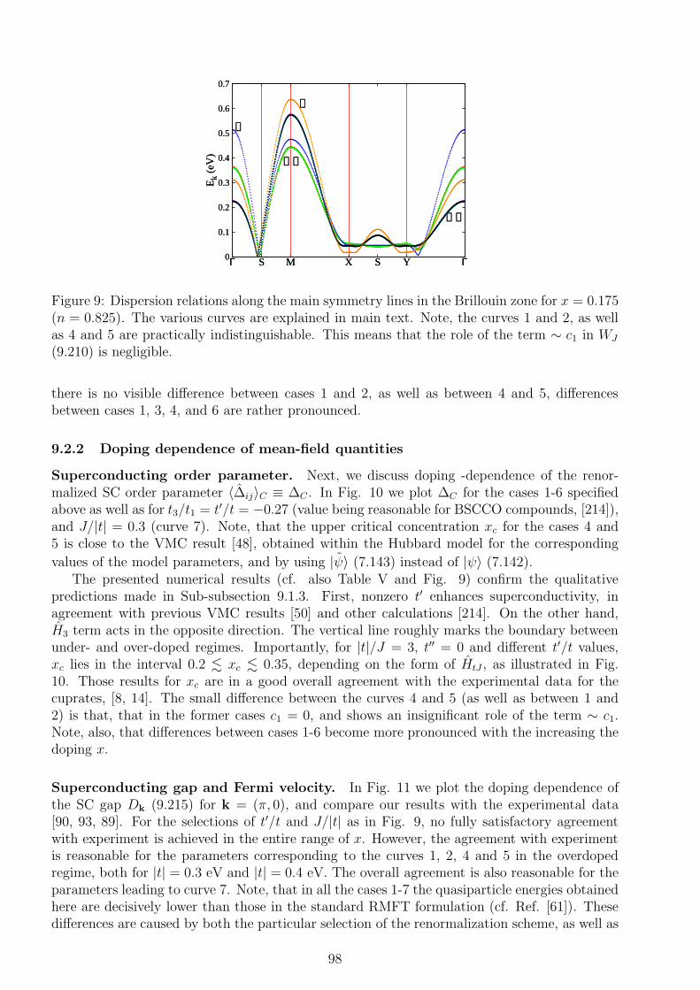
0
0.1
0.2
0.3
0.4
0.5
0.6
0.7
Γ S M X S Y Γ
Ek
(eV
)
➀➁
➂
➃➄
➅
0
0.1
0.2
0.3
0.4
0.5
0.6
0.7
Γ S M X S Y Γ
Ek
(eV
)
➀➁
➂
➃➄
➅
Figure 9: Dispersion relations along the main symmetry lines in the Brillouin zone for x = 0.175(n = 0.825). The various curves are explained in main text. Note, the curves 1 and 2, as wellas 4 and 5 are practically indistinguishable. This means that the role of the term ∼ c1 in WJ
(9.210) is negligible.
there is no visible difference between cases 1 and 2, as well as between 4 and 5, differencesbetween cases 1, 3, 4, and 6 are rather pronounced.
9.2.2 Doping dependence of mean-field quantities
Superconducting order parameter. Next, we discuss doping -dependence of the renor-malized SC order parameter 〈∆ij〉C ≡ ∆C . In Fig. 10 we plot ∆C for the cases 1-6 specifiedabove as well as for t3/t1 = t′/t = −0.27 (value being reasonable for BSCCO compounds, [214]),and J/|t| = 0.3 (curve 7). Note, that the upper critical concentration xc for the cases 4 and5 is close to the VMC result [48], obtained within the Hubbard model for the corresponding
values of the model parameters, and by using ˜|ψ〉 (7.143) instead of |ψ〉 (7.142).The presented numerical results (cf. also Table V and Fig. 9) confirm the qualitative
predictions made in Sub-subsection 9.1.3. First, nonzero t′ enhances superconductivity, inagreement with previous VMC results [50] and other calculations [214]. On the other hand,H3 term acts in the opposite direction. The vertical line roughly marks the boundary betweenunder- and over-doped regimes. Importantly, for |t|/J = 3, t′′ = 0 and different t′/t values,xc lies in the interval 0.2 . xc . 0.35, depending on the form of HtJ , as illustrated in Fig.10. Those results for xc are in a good overall agreement with the experimental data for thecuprates, [8, 14]. The small difference between the curves 4 and 5 (as well as between 1 and2) is that, that in the former cases c1 = 0, and shows an insignificant role of the term ∼ c1.Note, also, that differences between cases 1-6 become more pronounced with the increasing thedoping x.
Superconducting gap and Fermi velocity. In Fig. 11 we plot the doping dependence ofthe SC gap Dk (9.215) for k = (π, 0), and compare our results with the experimental data[90, 93, 89]. For the selections of t′/t and J/|t| as in Fig. 9, no fully satisfactory agreementwith experiment is achieved in the entire range of x. However, the agreement with experimentis reasonable for the parameters corresponding to the curves 1, 2, 4 and 5 in the overdopedregime, both for |t| = 0.3 eV and |t| = 0.4 eV. The overall agreement is also reasonable for theparameters leading to curve 7. Note, that in all the cases 1-7 the quasiparticle energies obtainedhere are decisively lower than those in the standard RMFT formulation (cf. Ref. [61]). Thesedifferences are caused by both the particular selection of the renormalization scheme, as well as
98
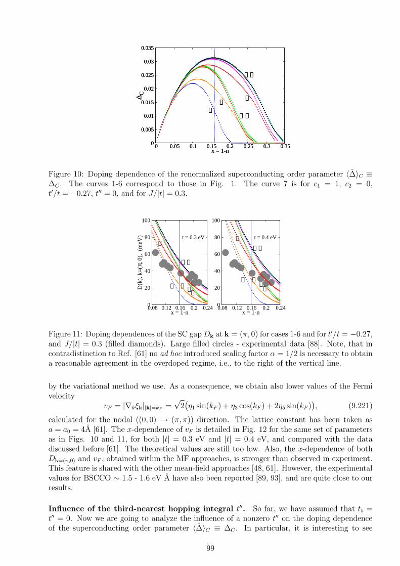
0
0.005
0.01
0.015
0.02
0.025
0.03
0.035
0 0.05 0.1 0.15 0.2 0.25 0.3 0.35∆ C
x = 1-n
➀➁➂
➅➆
➃➄
0
0.005
0.01
0.015
0.02
0.025
0.03
0.035
0 0.05 0.1 0.15 0.2 0.25 0.3 0.35∆ C
x = 1-n
➀➁➂
➅➆
➃➄
Figure 10: Doping dependence of the renormalized superconducting order parameter 〈∆〉C ≡∆C . The curves 1-6 correspond to those in Fig. 1. The curve 7 is for c1 = 1, c2 = 0,t′/t = −0.27, t′′ = 0, and for J/|t| = 0.3.
0
20
40
60
80
100
0.08 0.12 0.16 0.2 0.24
D(k
), k
=(π
, 0),
(m
eV)
x = 1-n
➀➁
➂ ➅
➃➄
➆t = 0.3 eV
0
20
40
60
80
100
0.08 0.12 0.16 0.2 0.24x = 1-n
➀➁
➂ ➅
➃➄
➆ t = 0.4 eV
Figure 11: Doping dependences of the SC gapDk at k = (π, 0) for cases 1-6 and for t′/t = −0.27,and J/|t| = 0.3 (filled diamonds). Large filled circles - experimental data [88]. Note, that incontradistinction to Ref. [61] no ad hoc introduced scaling factor α = 1/2 is necessary to obtaina reasonable agreement in the overdoped regime, i.e., to the right of the vertical line.
by the variational method we use. As a consequence, we obtain also lower values of the Fermivelocity
vF = |∇kξk||k|=kF=
√2(
η1 sin(kF ) + η3 cos(kF ) + 2η5 sin(kF ))
, (9.221)
calculated for the nodal ((0, 0) → (π, π)) direction. The lattice constant has been taken asa = a0 = 4A [61]. The x-dependence of vF is detailed in Fig. 12 for the same set of parametersas in Figs. 10 and 11, for both |t| = 0.3 eV and |t| = 0.4 eV, and compared with the datadiscussed before [61]. The theoretical values are still too low. Also, the x-dependence of bothDk=(π,0) and vF , obtained within the MF approaches, is stronger than observed in experiment.This feature is shared with the other mean-field approaches [48, 61]. However, the experimentalvalues for BSCCO ∼ 1.5 - 1.6 eV A have also been reported [89, 93], and are quite close to ourresults.
Influence of the third-nearest hopping integral t′′. So far, we have assumed that t5 =t′′ = 0. Now we are going to analyze the influence of a nonzero t′′ on the doping dependenceof the superconducting order parameter 〈∆〉C ≡ ∆C . In particular, it is interesting to see
99
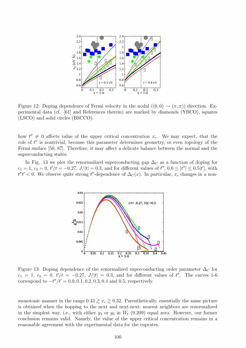
0.6
0.8
1
1.2
1.4
1.6
1.8
2
2.2
2.4
0 0.1 0.2 0.3
v F (
eV A
)
x = 1-n
➀➂
°
➃ ➄
➁➅
➆t = 0.3 eV
0.6
0.8
1
1.2
1.4
1.6
1.8
2
2.2
2.4
0 0.1 0.2 0.3x = 1-n
➀
➂
➃➄
➁
➆
t = 0.4 eV
➅
Figure 12: Doping dependence of Fermi velocity in the nodal ((0, 0) → (π, π)) direction. Ex-perimental data (cf. [61] and References therein) are marked by diamonds (YBCO), squares(LSCO) and solid circles (BSCCO).
how t′′ 6= 0 affects value of the upper critical concentration xc. We may expect, that therole of t′′ is nontrivial, because this parameter determines geometry, or even topology of theFermi surface [50, 87]. Therefore, it may affect a delicate balance between the normal and thesuperconducting states.
In Fig. 13 we plot the renormalized superconducting gap ∆C as a function of doping forc1 = 1, c2 = 0, t′/t = −0.27, J/|t| = 0.3, and for different values of t′′, 0.0 ≤ |t′′| ≤ 0.5|t′|, witht′′t′ < 0. We observe quite strong t′′-dependence of ∆C(x). In particular, xc changes in a non-
0
0.005
0.01
0.015
0.02
0.025
0.03
0 0.05 0.1 0.15 0.2 0.25 0.3 0.35 0.4 0.45
g∆ ∆
x = 1-n
➊
➌
➎
➏➋
➍
t,/t= -0.27, J/|t| =0.3
0
0.005
0.01
0.015
0.02
0.025
0.03
0 0.05 0.1 0.15 0.2 0.25 0.3 0.35 0.4 0.45
g∆ ∆
x = 1-n
➊
➌
➎
➏➋
➍
t,/t= -0.27, J/|t| =0.3
Figure 13: Doping dependence of the renormalized superconducting order parameter ∆C forc1 = 1, c2 = 0, t′/t = −0.27, J/|t| = 0.3, and for different values of t′′. The curves 1-6correspond to −t′′/t′ = 0.0, 0.1, 0.2, 0.3, 0.4 and 0.5, respectively.
monotonic manner in the range 0.43 & xc & 0.32. Parenthetically, essentially the same pictureis obtained when the hopping to the next and next-next- nearest neighbors are renormalizedin the simplest way, i.e., with either y3 or y5 in Wt (9.209) equal zero. However, our formerconclusion remains valid. Namely, the value of the upper critical concentration remains in areasonable agreement with the experimental data for the cuprates.
100

9.2.3 Dependence of upper critical concentration on value of exchange integral J
To provide an additional support for our conclusions, in Table VI we list the values of xc asa function of J , for either t′/t = −0.1 (considered to be relevant to the LSCO compound, [8])or t′/t = −0.27 (value that seems to be more relevant for BSCCO compound).57 Let us note,that the J- dependence of xc is substantial; critical concentration is roughly proportional to J .
Table VI. Upper critical concentration xc vs. exchange integral J , for either t′ = −0.27t ort′ = −0.1t. The symbols A (B) label the cases c2 = 0 and c1 = 0 (c1 = 1), respectively,
whereas C means that c1 = c2 = 1.
J/|t| 0.2 0.3 0.333 0.375 0.4t′/t = −0.1 A 0.18 0.26 0.29 0.32 0.33t′/t = −0.27 A 0.2 0.31 0.34 0.38 0.4t′/t = −0.1 B 0.18 0.27 0.3 0.33 0.35t′/t = −0.27 B 0.2 0.33 0.36 0.4 0.42t′/t = −0.1 C 0.15 0.21 0.22 0.24 0.25t′/t = −0.27 C 0.15 0.23 0.26 0.28 0.29
57Such selection of the values of t′/t ratio may seem to be rather arbitrary. The problem of choice of thevalues of model parameters for the specific compound is very nontrivial, and will not be discussed in the presentThesis.
101
10 Summary and discussion
10.1 Summary
The aim of this Thesis has been twofold. Our original aim was to provide a description of theselected properties of the cuprate superconductors within the renormalized mean-field theory(RMFT) of the t-J model. This topic was discussed in detail in part III. As a ’side subject’of this investigation, we have developed a new method of approach, which is based on themaximum entropy (MaxEnt) principle, and which allows to treat MF models considered herein a way which is both internally consistent and optimal from the point of view of statisticalphysics.
The method is presented in detail in Part II of the Thesis. The formal results presented thereare of general validity. Namely, our approach is applicable to any lattice fermion or spin model,and generalization to the case of lattice boson systems is also possible in principle. BecausePart II has got its own Summary (Section 5), therefore below we summarize and overview onlythe contents of Part III.
10.1.1 Comparison of present variational method and non-variational approachbased on self-consistent equations
The formal method developed in Part II has been applied in Part III to the RMFT of thet-J model. First, on the example of the mean-field treatment of the simplest form of the t-JHamiltonian, we have compared two distinct ways of solving mean-field models: the presentvariational (var) method, and the non-variational approach based on the Bogoliubov-de Gennes(BdG) self-consistent (s-c) equations. The latter approach to RMFT has been used by manyAuthors in their studies of various symmetry-broken states encountered in the cuprates [63,73, 74, 75, 78] and elsewhere. Our results show clearly, that there are nontrivial quantitative,and sometimes even qualitative differences between the var and the s-c approach; therefore,those two methods cannot be regarded as equivalent. Together with some purely theoreticalarguments in favor of the var approach, discussed in Part II of the Thesis, this observation leadsus to the following conclusion: the s-c method should be abandoned in the future analysis ofstrongly correlated systems, and its existing results should be re-examined within the presentvar approach.
10.1.2 Comparison of different renormalization schemes
We have compared various RMFT Hamiltonians, differing by the way in which correlatedaverages are approximated, i.e., differing by the applied renormalization schemes (RS). It turnsout, that differences between various RS are rather pronounced, for both the var, and for thes-c method. Therefore, also the energy difference between various symmetry-broken statesmay strongly depend on the particular choice of RMFT scheme. Because the value of theground state energy (or the free energy) usually serves as the criterion for selecting the optimalmean-field state, the (in)stability of complex states such as the stripe phases [73, 74, 75] or thevalence-bond solid phase [78] may be an artifact of a particular version of RS that has beenused. This scenario seems to be even more likely due to the circumstance, that the energydifferences between the latter states and some reference state (i.e., homogeneous RVB solution)are usually small.
102
10.1.3 Optimal renormalization scheme
Eventually, we have selected the renormalization scheme (RS) of Fukushima [76], which, in ouropinion is the optimal one among RS considered in the present Thesis. Our choice has beenmotivated by a transparent way in which this RS is constructed, and the fact that the formalismof Ref. [76] may be relatively easily applied to an arbitrary version of the t-J Hamiltonian, e.g.the complete form of the latter, in which the three-site terms are included. Also, the agreementof the results obtained previously by Fukushima with those of the VMC method speak in favorof this particular RS.
Next, the RS of Ref. [76] has been applied to investigate various forms of the t-J Hamilto-nian, and for different values of model parameters, i.e., t, t′, t′′, and J/t. Our results agree quitewell with those of the earlier VMC studies (some obtained for the Hubbard model but for thecorresponding values of the model parameters, cf. e.g. [48]). For example, doping dependenceof the superconducting order parameter, and, in particular, value of the upper critical concen-tration xc are close to the VMC results. Also, we have observed the tendency that the nonzeronext-nearest neighbor hopping integral t′, enhances superconductivity, whereas the three-siteterm of the t-J Hamiltonian (frequently neglected in the literature) acts in the opposite di-rection. The influence of the third-nearest neighbor hopping t′′ is more complicated; t′′ 6= 0enhances superconductivity as compared to the t′′ = 0 case. However, xc depends then on t′′ ina non-monotonic manner. Also, selected spectral features, e.g. the superconducting gap Dk atk = (π, 0) or the Fermi velocity vF = |∇kξk||k|=kF
in the nodal ((0, 0) → (π, π)) direction havebeen studied and found to be in a semiquantitative agreement with the ARPES measurements[90, 91, 93], at least in the overdoped regime.
In general, the results obtained within the RMFT turned out to depend quite strongly onboth the various forms of the original t-J model, as well as on choice of the model parameters.The right choice of the values of model parameters is nontrivial; the values selected here areidentical or close to those selected frequently in the literature.
10.1.4 Limitations of RMFT approach
It must be emphasized here, that even though the RMFT of the t-J model proved to be quitesuccessful in predicting many physical properties of high-Tc cuprate superconductors, it stillcertainly cannot be regarded as a complete description of those compounds.
First, let us note, that the choice of the mean-fields which may have non-zero optimal(equilibrium) values, i.e being relevant for the problem at hand, is dictated mostly by theexperiment. For example, there is a strong experimental evidence in favor of dx2−y2 symmetryof the superconducting order parameter in the bulk of the cuprates, and very sparse for otherpossible, e.g. dx2−y2 + idxy [12]. Therefore, usually from the very beginning we exclude ’byhand’ the more exotic symmetries of the superconducting order parameter. However, fromthe point of view of a model description, certain symmetry-breaking patterns excluded by theexperimental data are certainly legitimate. Obviously, there is no certainty, that the solutionsuggested by experiment would turn out to be the optimal one (i.e., of the lowest energy)within our MF model for the reasonable choice of the model parameters. In connection withthis, it must be emphasized, that one of the possible extensions of the present approach tothe case a magnetically-ordered states leads to the results which are unphysical in the contextof the physics of cuprates. Namely, recently it has been shown by Kaczmarczyk et al. [216],that within the so-called local spin-dependent version of the formalism of Ref. [76], the normalstate with saturated, uniform magnetic polarization has lower energy then any state analyzedin the present Thesis, for the same values of the model parameters. We may still hope, thatthe application of an alternative ’local spin-independent constraint’ of Ref. [76] would lead todifferent results for the magnetic states. Also, the unphysical predictions may be attributed
103
to the fact, that the effects of the orbital magnetism has been neglected. The same problemis very likely to be present in other versions of RMFT formalism, i.e., for other versions ofGutzwiller approximation (other renormalization schemes).
RMFT leads to description in terms of an effective, single-particle Hamiltonian. This featureallows us to address easily all the single-particle properties (e.g. the Fermi surface existence,quasiparticle dispersion observed in ARPES experiments, or symmetry of the order parameter),but obviously must be regarded as (rather crude) approximation to the complete descriptionof the real, strongly-correlated system. Also, for the normal state, single-particle models leadto the description in the spirit of the Landau theory of Fermi liquids (presence of heavy quasi-particles). The latter theory, however, is regarded legitimate at most in the overdoped regimeof the phase diagram of the cuprates, as was presented here.
Moreover, as may be intuitively expected, and as has been formally shown in Part II, RMFTof the t-J model (similarly to any simple MF approach) remains in the paradigm of the Landau(-Ginzburg-Wilson) theory of phase transitions, with all consequences of this fact. For example,RMFT may be incapable of providing a proper description of those quantum states, which haveno long-range static order.
Another point is an important role of fluctuations (both quantum and thermal) of theorder parameters. This issue is probably crucial for understanding of either the nature of thepseudogap phase (cf. e.g. [218]), or the fate of the superconducting state at low doping, anda disappearance of the antiferromagnetic long-range order with the increasing doping. Still,inclusion of fluctuations on the mean-fields level seems to be a highly nontrivial task. Despitesome attempts to treat fluctuation within the present method we have made (see the discussionin Subsection 12.1), resolution of this problem remains unclear for us at the moment.
10.2 Outlook and possible extensions of present work
The approach presented in this Thesis may be generalized and improved in several ways, whichare listed below.
10.2.1 Approximation-free evaluation of correlated averages
What seems to be the most important modification of the present formalism, is the implemen-tation of a more accurate way of evaluating the correlated averages 〈O〉C (7.145), i.e., averagesof operators calculated with respect to the correlated state |Ψ0〉 = PC |Ψ0〉 (7.140). Even if anexact evaluation of 〈O〉C may turn out to be impossible in practice, still, we should at least tryto estimate the error in a rigorous way. In this manner, it might be possible to obtain an exactupper bound for the ground state energy of the t-J Hamiltonian.
10.2.2 Other trial correlated states
In connection with the statements of the previous Sub-subsection, we should mention, that theRVB state used here (Eqn. (7.138)) may be not sufficient as a complete trial variational state forthe t-J model. Namely, the correlation operator PC in the correlated trial state (7.140) shouldbelong to the same class as the Hamiltonian, for which this trial state serves as an approximateground state. By this, we understand the following: in contrast to the Hubbard model, the t-Jmodel contains intersite interaction terms. Consequently, the correlator should also belong tothe class of inter-site operators, which is not the case for the local Gutzwiller projector P (6.129)[217]. This observation suggests, that within the RMFT approach we should use variationaltrial states of a more general form, e.g. containing various Jastrow correlators [33, 181]. Suchstates have been already used in some of the VMC studies [53].
104

10.2.3 Higher-order corrections to t-J Hamiltonian
As discussed in Section 6.136, t-J Hamiltonian is derived from the Hubbard Hamiltonian in thestrong coupling limit (t ≪ U) by using canonical transformation. When doing this, we retainonly terms ∼ t (kinetic energy part) and ∼ t·(t/U) (interaction part). However, using canonicaltransformation we may construct effective Hamiltonians, which contain terms of higher order,i.e., t · (t/U)k. On the other hand, for the cuprates the reasonable value of t/U is about 1/12,hence this parameter is not small enough to a priori disregard the higher-order terms in theeffective Hamiltonian. Therefore, investigation of such effective Hamiltonians (at least the onecontaining terms up to ∼ t · (t/U)3, e.g. the ring-exchange terms) by means of the appropriatemean-field approach seems to be desirable, although it may turn out cumbersome.
10.2.4 Analysis a nonzero temperature
The next problem, which also seems to be important as a subject of future analysis, is anextension of the RMFT approach to arbitrary temperatures. Such formalism would allow usto study large part of x-T phase diagram of the cuprates, and, in particular, to determine thecritical temperature Tc as a function of doping. As mentioned in Section 7.4.1, attempts toextend Gutzwiller approximation (GA) to T > 0 have been made in the case of the Hubbardmodel [209, 210, 211]. Recently, a similar approach has been proposed for the t-J-U model[202], hence it is applicable also to the RMFT of the t-J model.
At first glance, it may seem that by using mean-field approach developed in this Thesis,it is legitimate to study RMFT at arbitrary value of T . Unfortunately, this is not the case.Although our method is an intrinsically finite-temperature approach, in the case of RMFT ofthe t-J model it is not expected to lead to physically reliable predictions at higher temperatures.This insufficiency is not caused by the flaws of the method, but rather by the nature and origin ofthe RMFT approach. The latter, as based on the Gutzwiller approximation, has been originallydevised to study the ground-state properties of the system. Therefore, in this Thesis, we haveaddressed only the low temperature case, kBT/J = 0.002, which is practically equivalent to thetrue T = 0 situation.
In order to treat consistently arbitrary temperatures, the original method of Gutzwillershould be modified. In our opinion, this problem has no satisfactory solution as yet, at leastin the case of the fully-projected trial states required for the t-J model. In particular, in thelatter case the formalism of Ref. [202] does not provide a acceptable solution, as discussed in[83].
Nonetheless, because our method is a natural and convenient formal basis for a finite-temperature mean-field analysis of any model of correlated lattice fermions, we hope that itmay be also used to construct an appropriate finite-temperature version of RMFT. We shouldsee the progress along this line in the near future.
10.2.5 More complex symmetry-broken states, lattice geometry, and band struc-ture
Another natural path to extend the present treatment would be to investigate a more com-plex lattice geometry and band structure. For example, bilayer structure and orthorhombicdistortion (lack of the C4v-symmetry of CuO2 planes, leading e.g. to the mixed d- and swave symmetry of the superconducting order parameter) may be quite easily included withinthe present formalism. Both features may be important for more realistic description of thecuprate superconductors.
Moreover, the ’classical phonons’, i.e., static lattice distortion [199, 204] may be implementedin a simple way within the present approach. This step may be important for the analysis of
105
the C4v-symmetry breaking, not only in the presence of the orthorhombic distortion, but alsospontaneous, as occurring for the x-y symmetric Hamiltonian in the normal state (Pomeranchukinstability, PI).
Next, apart from the homogeneous, non magnetic resonating-valence bond RVB supercon-ducting state, C4v-symmetry broken normal PI state, and simple staggered-flux state (SF)discussed in the present Thesis, other symmetry-broken states may be also studied. In par-ticular, the antiferromagnetic long-range order (AF), its competition or coexistence with boththe superconducting, staggered-flux or charge order are among those physical properties, whichcan be relatively easily described by the present MF approach. Work along these lines is beingcarried out in our group at present and will be reported separately.
Finally, let us note, that the investigation of yet more complicated states, like the stripephases or valence bond solid phase [78] within the formalism presented in this Thesis should leadto quantitatively or even qualitatively new results. Also, no attempt to describe the pseudogapstate has been made in the present Thesis.
10.2.6 Ginzburg-Landau potential
Using the results of Section 4.5, we can construct the Ginzburg-Landau (G-L) free-energypotentials (i.e., a discrete version of the original G-L functional) for the RMFT Hamiltonians.The Ginzburg-Landau picture for the RMFT approach may be helpful to study, or at leastto visualize, the normal-to-superconducting transition at xc. It would be interesting then tocompare the Ginzburg-Landau approach resulting from the microscopic RMFT description withthe phenomenological G-L theory as given e.g. in Ref. [219].
106
Part IV
Appendices and supplementarymaterial
11 Appendices
11.1 Appendix A: Deficiencies of approach not based on the methodof Lagrange multipliers
In Sub-subsection 4.3.3, we have point out some difficulties arising when one tries to applythe MaxEnt principle to the MF approach, but without invoking the method of Lagrangemultipliers. For completeness, below we present further comments on that issue.
At first, let us assume, that the eigenbasis of the (yet unknown) MF density operator ρ,
i.e., |i〉DH
i=1, is ~A-independent. Using |i〉DH
i=1, Sλ (4.9) can be written as
S = −∑
i
(
pi ln pi + β[K( ~A)]iipi + ω(pi − 1/DH))
, (11.222)
with [O]ii ≡ 〈i|O|i〉 and [K( ~A)]ii = [H( ~A)]ii −µ[N ]ii. In the present situation, Eqs. (4.12), i.e.,
Tr[ρAs] = 〈As〉 = As =∑
i
pi[As]ii =∑
i
pi〈i|As|i〉, (11.223)
allows us to eliminate As in favor of the probabilities pi, and the latter remain then the onlyindependent variables. Consequently, the necessary conditions for S to have an extremum readnow
∂S∂pk
= 0 = − ln pk − β[K( ~A)]kk − ω − 1 − β∑
i
pi
∑
s
[K( ~A)]ii∂As
[As]kk, (11.224)
for k = 1, 2, . . . , D and with the normalization condition (∑
i pi = 1) imposed. However,equations (11.224) cannot be solved analytically, and thus an explicit functional dependence of
pi on T, V (or Λ), µ,~h, . . . cannot be obtained. Eqs. (11.224) can be rewritten as
pk = Z−1 exp
(
−β([K( ~A)]kk +∑
i
pi
∑
s
∂[K( ~A)]ii∂As
[As]kk
)
. (11.225)
Obviously, the probability distribution given by (11.225) is not of a canonical (Gibbs) form.By defining
−λs =
⟨
K( ~A)
∂As
⟩
=∑
i
pi[K( ~A)]ii∂As
, (11.226)
we can rewrite (11.225) as
pk = Z−1 exp(
− β([K( ~A)]kk −∑
s
λs[As]kk
)
. (11.227)
For a given ~A, pk (11.227) has a form similar to that of qk, given by diagonal elements of ρλ
(4.29), i.e.,
qk = Z−1λ exp
(
− β(
[K( ~A)]kk −∑
s
λs([As]kk −As))
)
, (11.228)
107
because the constant (independent of k) term present in qk (11.228) and absent in pk (11.227)can be absorbed in Z−1
λ .Apparently, by defining (11.226), we have taken a step towards approach of Subsections
4.3 and 4.4. However, first, a route presented here ignores the algebraic structure of thequantum model. It should be a posteriori checked, if indeed the assumption we have made,i.e., the existence of an ~A -independent eigenbasis of ρ (which has been used to computetrace appearing in the above formulas) does not lead to contradiction. This task, however,is enormously complicated, if not entirely impossible. On the other hand, we cannot assumea priori, that MF grand Hamiltonian K( ~A) commutes with the density matrix, therefore theeigenbasis of the former operator cannot serve as the eigenbasis of the latter.
If the eigenbasis of ρ is not ~A-independent, the reasoning leading to most of the aboveformulas ceases to valid. To see that, let us expand eigenvectors of ρ in some ~A-independentbasis, i.e., |i( ~A)〉 =
∑
l cil(~A)|l〉 and next rewrite (11.223) in a form
As =∑
i
pi[As]ii =∑
i
pi〈i( ~A)|As|i( ~A)〉 =∑
i
pi
∑
j,l
c∗ij(~A)cil( ~A)〈j|As|l〉. (11.229)
Apart from very special cases, As variables cannot be expressed as any explicitly known func-tions of pi.
11.2 Appendix B: Equivalence of two alternative expressions for thesecond derivative of thermodynamic grand potential Ω
Below we show the equivalence of two alternative formulas (Eqn. (4.52) and Eqn. (4.53))for the second derivative of the thermodynamic potential Ω with respect to thermodynamicvariables x1, x2 ∈ T, V, µ,~h, . . .. Eqs. (4.52) and (4.53) read, respectively
∂2Ω
∂x2∂x1
=∂
∂x2
(
∂F∂x1
)
0
=
(
∂2F∂x2∂x1
)
0
+∑
s
(
∂2F∂x1∂As
)
0
∂As0
∂x2
+
(
∂2F∂x1∂λs
)
0
∂λs0
∂x2
(11.230)
∂2Ω
∂x2∂x1
=∂
∂x2
[
(
∂F∂x1
)
0
+∑
s
(
∂F∂As
)
0
∂As0
∂x1
+
(
∂F∂λs
)
0
∂λs0
∂x1
]
=
(
∂2F∂x1∂x2
)
0
+∑
s
(
∂2F∂x1∂As
)
0
∂As0
∂x2
+
(
∂2F∂x1∂λs
)
0
∂λs0
∂x2
+∑
s
(
∂2F∂x2∂As
)
0
∂As0
∂x1
+
(
∂2F∂x2∂λs
)
0
∂λs0
∂x1
+∑
s,t
(
∂2F∂At∂As
)
0
∂As0
∂x1
∂At0
∂x2
+
(
∂2F∂As∂λt
)
0
∂As0
∂x1
∂λt0
∂x2
+
(
∂2F∂As∂λt
)
0
∂As0
∂x2
∂λt0
∂x1
+
(
∂2F∂λs∂λt
)
0
∂λs0
∂x1
∂λt0
∂x2
+∑
s
(
∂F∂As
)
0
∂2As0
∂x1∂x2+
(
∂F∂λs
)
0
∂2λs0
∂x1∂x2
. (11.231)
The r.h.s. of (11.230) is asymmetric with respect to x1 and x2. It seems also to be incompatiblewith (11.231). However, both features are only apparent. Indeed, for any s we have
0 =∂
∂x2
(
∂F∂As
)
0
=
(
∂2F∂As∂x2
)
0
+∑
t
(
∂2F∂At∂As
)
0
∂At0
∂x2+
(
∂2F∂As∂λt
)
0
∂λt0
∂x2
. (11.232)
108
Multiplying (11.232) by ∂As0/∂x1 and summing over s we obtain
0 =∑
s
(
∂2F∂As∂x2
)
0
∂As0
∂x1+∑
s,t
(
∂2F∂At∂As
)
0
∂As0
∂x1
∂At0
∂x2+
(
∂2F∂As∂λt
)
0
∂As0
∂x1
∂λt0
∂x2
.
(11.233)Analogously,
0 =∂
∂x2
(
∂F∂λs
)
0
=
(
∂2F∂λs∂x2
)
0
+∑
t
(
∂2F∂At∂λs
)
0
∂At0
∂x2+
(
∂2F∂λt∂λs
)
0
∂λt0
∂x2
. (11.234)
Multiplying (11.234) by ∂λs0/∂x1 and summing over s we obtain
0 =
(
∂2F∂As∂x2
)
0
∂λs0
∂x1
+∑
s,t
(
∂2F∂At∂λs
)
0
∂λs0
∂x1
∂At0
∂x2
+
(
∂2F∂λs∂λt
)
0
∂λs0
∂x1
∂λt0
∂x2
. (11.235)
Changing dummy indices (e.g. s↔ t) if necessary, we identify in (11.231) the terms appearingon the r.h.s. of Eqn. (11.233) and (11.235). Note also, that the last line of (11.231) vanishesdue to (4.34). This completes the proof of the equivalence of Eqn. (11.230) and Eqn. (11.231)(or Eqn. (4.52) and Eqn. (4.53)).
11.3 Appendix C: Generalized thermodynamic potentials and Leg-
endre transformations
Natural thermodynamic variables of Fz( ~A) ≡ Fz(T, V, µ,~h; ~A) (4.44) are identical with those
of the thermodynamic grand potential Ω = Ω(T, V, µ,~h). The relation between Fz and Ω givenby Eqs. (4.47), i.e.,
Fz( ~A0(T, V, µ,~h);T, V, µ,~h) = Ω(T, V, µ,~h), (11.236)
is same as in the original Landau theory. Therefore Fz( ~A) corresponds to Ω(µ, T, η), Eqn.(146.3) of Ref. [148]. Nonetheless, within the original Landau approach, other generalizedthermodynamic potentials are also used, e.g. Φ(p, T, η), Eqn. (143.1) of [148] (’Gibbs free
energy potential’), denoted here as G(T, p,N,~h; ~A). Because within the phenomenological ap-proach of Landau, there exist no underlying microscopic mean-field model, one has a freedomto choose those thermodynamic variables and the corresponding generalized thermodynamicpotential, which are the most convenient (or natural) for the considered problem. On the
other hand, within the present approach, Fz(T, V, µ,~h; ~A), appearing as the result of the MFgrand-canonical description, has a privileged status. Similarly, free energy Landau potentialFz(T, V,~h; ~A) would be a natural choice for the canonical ensemble, in a situation when theaverage particle number does not appear as one of the mean fields, e.g. for the MF model ofthe spin system analyzed in Section 12.3.
If we want to define here the analog of Φ(p, T ; η) of Landau, we have to make Legendre
transformations V ↔ p, µ ↔ N leading from T, V, µ,~h to the new set of independent thermo-
dynamic variables, i.e., T, p,N,~h. However, in order to do that, we have to construct first theequilibrium thermodynamic potentials along the lines of Subsection 4.6. Both p and N becomethen functions of T, V, µ, and ~h, given by the respective derivatives of Ω = Ω(T, V, µ,~h), cf. Eqs.
(4.48). By inverting those relations, we obtain V (T, p,N,~h) and µ(T, p,N,~h). Consequently,
G(T, p,N,~h; ~A) should be defined as
G(T, p,N,~h; ~A) = Fz(T, V (T, p,N,~h), µ(T, p,N,~h),~h; ~A) + pV + µN. (11.237)
109
In the above, N denotes the equilibrium value of the average particle number, and not thecorresponding mean field A1 = 〈N〉z. In analogy to Eqn. (11.236), we have
G(T, p,N,~h; ~AG0 (T, p,N,~h)) = G(T, p,N,~h). (11.238)
Superscript G indicates that now ~AG0 depend on T, p,N,~h, and not on T, V, µ,~h. Even if within
the present approach, G(T, p,N,~h; ~A) appears in a less natural manner than Fz(T, V, µ,~h; ~A),it may be more convenient in a situation, when the average particle number and pressure arefixed. If needed, it may be constructed as discussed above.
11.4 Appendix D: Renormalization scheme of Fukushima
Below we provide a more detailed analysis of the RS proposed by Fukushima in Ref. [76].Within this formalism, Gutzwiller projection operator (projector) P (6.129) is replaced by thefollowing correlation operator (correlator)58
PC = P (F ) =∏
i
(λFi↑)
ni↑2 (λF
i↓)n
i↓2 (1 − ni↑ni↓). (11.239)
As a consequence, the correlated trial state (7.141) is replaced by |Ψ〉 (7.142) of the form
|Ψ〉 = P (F )(λFi↑, λ
Fi↓)|Ψ0〉 =
∏
i
(λFi↑)
ni↑2 (λF
i↓)n
i↓2 (1 − ni↑ni↓)|Ψ0〉. (11.240)
With the help of |Ψ〉 (11.240) we define the correlated average (Eqn. (7.145)) as
〈O〉C ≡ 〈Ψ|O|Ψ〉〈Ψ|Ψ〉 =
〈Ψ0|PCOPC |Ψ0〉〈Ψ0|P 2
C |Ψ0〉. (11.241)
P (F ) differs from P (6.129) by presence of the fugacity factors59 λFiσ, see also Eqs. (7.142). Such
modification of the standard Gutzwiller projector allows us to enforce the following condition:the uncorrelated average number of electrons on each lattice site i and each spin direction σ isequal to the corresponding correlated average, computed within the approximation of Ref. [76](see below). Explicitly,
〈niσ〉appC = 〈niσ〉. (11.242)
There exist few variants of the formalism of Ref. [76]. The condition (11.242) refers to the’local spin-dependent constraint’. Alternatively, one may choose the ’local spin-independentconstraint’. In such case, we replace niσ in (11.242) by ni ≡ ni↑ + ni↓. Consequently, thenwe have only one fugacity factor λF
i for each site. There exist also the corresponding ’global’,i.e., site-independent variants of both ’spin-dependent’ and ’spin-independent’ constraint, i.e.,with niσ (ni) in (11.242) replaced by
∑
i niσ = Nσ and∑
i ni = N , respectively. However, fornon-magnetic (ni↑ = ni↓) and homogeneous (niσ = njσ) solutions analyzed in this Thesis, allthe above mentioned variants of the RS of Fukushima are equivalent. Therefore, in our case,the condition (11.242) reduces to
〈N〉appC = 〈N〉 = N. (11.243)
Note, that when |Ψ0〉 is an eigenstate of N , projection does not change N , because [N, P ] = 0.However, this is not the case for |Ψ0〉 of the BCS form, because the latter is an eigenstate of
58All formulas in this Appendix are provided by using our own notation, which differs from that of the originalreference [76].
59Please not confuse those quantities with the Lagrange multipliers introduced within our formalism.
110

the Hamiltonian which does not commute with N , [N, HBCS] 6= 0. Also, without the fugacity
factors λFiσ in the projector, due to the approximation used to compute W ( ~A) (7.168), we would
usually have 〈N〉appC 6= 〈N〉 even if |Ψ0〉 appearing in |Ψ〉 = P (F )|Ψ0〉 (11.240) was an eigenstate
of N .60 Coming back to Eqn. (11.242), we can rewrite it in a form
〈niσ〉C =
⟨
λFiσniσ
(
1 − niσ
)∏
l 6=i
(
P(F )l
)2⟩
⟨∏
l
(
P(F )l
)2⟩ (11.244)
Approximate way of computing (11.244) consist of neglecting all inter-site contractions. Thisyields
〈niσ〉C ≈ 〈niσ〉appC =
λFiσ
(
1 − niσ
)
Ξi· niσ, (11.245)
where
Ξi =⟨(
P(F )i
)2⟩= (1 − ni↑)(1 − ni↓) + λF
i↑ni↑(1 − ni↓) + λFi↓ni↓(1 − ni↑). (11.246)
By solving (11.245) and (11.246) we obtain
λFiσ =
1 − niσ
1 − ni, Ξi =
(1 − ni↑)(1 − ni↓)
1 − ni. (11.247)
Now, using the above results, one can compute various correlated averages (11.241). Note, thatthe method of Ref. [76] can be relatively easily applied to the full form of the t-J Hamiltonian(6.127), as well as to the more complicated symmetry-broken states. Here, we will not providedetails of this procedure, the Reader is encouraged to consult the original paper. Formula for〈H3〉app
C , not appearing in the latter paper, is too lengthy to be reproduced here, but for thespecial (homogeneous, nonmagnetic) case it is provided in Section 9 (Eqn. (9.211)). Also, theaverage of the full kinetic exchange term, Eqn. (9.210) is a special case of the general expressionfor 〈Si · Sj − 1
4ninj〉app
C . As an example, we invoke only the formula for the renormalizationhopping amplitude
〈c†iσcjσ〉appC =
√
1 − ni
1 − niσ
√
1 − nj
1 − njσ
(
χijσ − χijσχijσχijσ + ∆ji∆ij
(1 − niσ)(1 − njσ)
)
, (11.248)
provided already in Subsection 7.5. Please note, that all formulas in Ref. [76] are provided upto the second order in the inter-site contractions χ∗
ij , ∆∗ij , and the estimated corrections are of
order of |χijσ|4 and |∆ij |4. Therefore, all the conditions of the form (11.242) are fulfilled to thesame accuracy. However, the results of Ref. [76] may be, at least in principle, systematicallyextended beyond the second order in χij and ∆ij.
60Let us note here, that the condition (11.243) can be also enforced in an alternative manner, cf. [220, 221]and References therein.
111
12 Supplements
12.1 Supplement A: Thermodynamic fluctuations and internal lim-itations of mean-field description
Below we provide the Reader with the analysis of thermodynamic fluctuations. This issue hasbeen omitted in the main text, as being weakly related to the main scope of the present Thesis.The problem is also quite nontrivial, due to the fact, the within the present approach two kindsof fluctuations are present. On the other hand, even incomplete analysis of the non-equilibriumsituation allows us to establish natural internal limitations on the validity of the mean-fieldapproach.
12.1.1 Probability of a non-equilibrium MF configuration
Following Landau [148], (see also [133]), we assume that the probability that our system remains
in a state characterized by a mean-field configuration ~A, for a given T, V, µ, and ~h is given by
w(T, V, µ,~h; ~A) ≡ w( ~A) ∼ exp(
−β∆ΩL(T, V, µ,~h; ~A))
. (12.249)
After Landau, by ∆ΩL(T, V, µ; ~A) we denote minimum work required to bring the system from~A0 to ~A in a reversible manner and assuming constant T , V , µ and external field(s) ~h. In whatfollows, it we will be shown that
∆ΩL(T, V, µ,~h; ~A) ≡ Fz(T, V, µ,~h; ~A) − Fz(T, V, µ,~h; ~A0), (12.250)
and, consequently thatw( ~A) ∼ exp
(
− βFz(T, V, µ,~h; ~A))
. (12.251)
In order to that, we make use of the results of Ref. [222].61 It will be shown, that Fz( ~A) may
be identified with the ’non-equilibrium grand potential’, Ωn( ~A). To define the latter quantity,
we start from a stable equilibrium situation characterized by ~A = ~A0 and fixed T , V , µ and ~h.If we want to deal with a reversible process, i.e., the sequence of equilibrium states, we mustintroduce additional, external forces. On the technical level, it may be realized by introducingadditional ’source’ terms of the form (−∑s ζsAs), which are added to the MF Hamiltonian
Hz( ~A) (4.42). We define also
Ψ( ~A) ≡ −β−1 ln Tr[
exp(
− β(Hz( ~A) −∑
s
ζsAs − µN))]
. (12.252)
For each ~A, values of the ’source fields’ ζs = ζs( ~A) will be determined from the condition, that~A is an equilibrium mean-field configuration in the presence of those additional forces, i.e., that∇AΨ( ~A) = 0. Then Ψ( ~A) (12.252) becomes a corresponding equilibrium grand potential for ~A.
Next, following Ref. [222], we define the non-equilibrium grand potential Ωn( ~A) as
Ωn( ~A) ≡ Ψ( ~A) − Uζ = Ψ( ~A) +∑
s
ζsAs. (12.253)
In the above, Uζ = 〈−∑s ζsAs〉z = −∑s ζsAs is the potential energy of the additional force
fields. To show that indeed Fz( ~A) is identical to Ωn( ~A), we have to invoke the results of
61Although in Ref. [222] the non-mean-field case is analyzed, and the free energy is used instead of a grandpotential, we follow closely the original reasoning of Leontovich and adapt it for the present purposes.
112
Subsection 4.8. Namely, after the self-consistency equations (4.41) are solved for each ~A,
MF Hamiltonians Hz( ~A) and Hz( ~A) −∑s ζs(~A)As belong to the same universality class, and
therefore differ only by a constant term∑
s ζs(~A)As. Indeed, in such situation, for each ~A, value
of λs appearing in Hz( ~A) is equal to the value of (λs+ζs ≡ λζs) appearing in Hz( ~A)−∑s ζs(
~A)As.We obtain a desired result due to obvious relation
Hz( ~A) −∑
s
ζs( ~A)As = H( ~A) −∑
s
λζs( ~A)
(
As − As
)
−∑
s
ζs( ~A)As. (12.254)
Consequently, for each ~A, also the corresponding functionals Fz( ~A) (4.44) and Ψ( ~A) (12.252)
differ only by the term∑
s ζsAs, i.e., Ψ( ~A) = Fz( ~A) −∑s ζsAs. Therefore, from (12.253) it
follows that Fz( ~A) = Ωn( ~A) and Ωn( ~A) − Fz(T, V, µ; ~A0) is equal to ∆ΩL(T, V, µ; ~A), as in
[148]. This proves Eqn. (12.250). In that way we have argued, that Fz( ~A), defined for a givenmicroscopic mean-field model according to Eqn. (4.44), may be consistently interpreted as aLandau potential.
12.1.2 ’Classical’ and ’quantum’ probability distributions
Invoking (12.249) or (12.251), we may define
p( ~A ≤ ~A ≤ ~A + d ~A) ≡ ϕ( ~A)d ~A, ϕ( ~A) = N−1 exp(−βFz( ~A)). (12.255)
~A is a random variable associated with ~A, and N is the normalization constant. In result, wedeal with two entirely different probability distributions. The first is given for each ~A by ρz( ~A).It yields a (conditional) probability of finding a system in a quantum state |i〉 provided that
values of the classical parameters are equal ~A (therefore, strictly speaking, we should write
|i( ~A)〉 instead of |i〉). The second probability distribution is ϕ( ~A) defined by (12.255), andrelated to the probability of a particular value of each of the ’classical’ quantities A1, . . . , AM .The latter variables may be regarded as constituting some kind of a ’classical phase space’.
12.1.3 Degenerate minima of Fz( ~A)
In the absence of an external, symmetry breaking field ~h (i.e., real magnetic field), ϕ( ~A) (12.255)is invariant with respect to the allowed symmetry transformations of the mean fields (orderparameters), exactly as in the original Landau approach. However, in the present case the
symmetry of ϕ( ~A) is inherited from microscopic MF Hamiltonian Hz( ~A). Namely, two micro-
states, |i( ~A′)〉 and |i( ~A′′)〉 with ~A′ and ~A′′ related by symmetry transformations (e.g. with
As for ~A′ and −As for ~A′′ if Fz( ~A) is even with respect to As), enter the corresponding par-
tition functions Zz( ~A′) and Zz( ~A′′)(4.42) with exactly the same weight. Consequently, we
have Zz( ~A′) = Zz( ~A′′) and Fz( ~A′) = Fz( ~A′′). This may be also interpreted from the point
of view of MaxEnt inference. Namely, if Hz( ~A′) = Hz( ~A′′), no prior information about the
symmetry breaking is encoded in Sλ, hence ~A′ is equivalent to ~A′′ and the resulting probabilitydistributions p1( ~A
′), . . . , pDH( ~A′) and p1( ~A′′), . . . , pDH
( ~A′′) are identical. As a consequence, the’classical’ average values of some of the mean-fields, which could be defined as
As ≡∫
DA
Asϕ( ~A)d ~A (12.256)
obtained using ϕ( ~A) are equal zero. This feature is obviously connected to the fact, thatthe symmetry should be explicitly broken before any classical fluctuations around the equilib-rium situation can be considered - classical situation corresponds to already broken symmetry.
113

Therefore, we have to replace ϕ( ~A) by some other, asymmetric function, ϕ( ~A) → ϕ( ~A). Unfor-tunately, in the general case there is no obvious prescription how to achieve this. One possibleway is to apply Gaussian approximation to ϕ( ~A) in the vicinity of one of the equivalent equi-
librium solutions, i.e., ~A = ~A0. Under certain conditions this step is legitimate, as discussedbelow. On the other hand, we may argue that if other regions of DA are also characterizedby large values of ϕ( ~A) (i.e., points in the vicinity of other degenerate minima of Fz( ~A)), theyare separated by very large energy barriers, and hence practically inaccessible for the systemcharacterized by ~A = ~A0.
This reminds us, that the problem of degenerate states, characterized by the same values of(generalized) thermodynamic potentials and leading to vanishing averages, is present not only innon-MF statistical physics, but also within the MF treatment, where it is only somehow ’sweptunder the carpet’. Obviously, this is not only the property of the microscopic MF models, it isalso present in the Landau theory.
12.1.4 Dual nature of fluctuations
Having both ρz( ~A) and ϕ( ~A) present in our formalism, we may consider two distinct kindsof fluctuations. Apart from the above mentioned ’classical’, there appear also ’quantum’ fluc-tuations. The magnitude of the former is proportional to second moments of ϕ( ~A), i.e., to
AsAt−As ·At. For a given ~A, the magnitude of the latter is proportional to Tr[(As−As)2ρz( ~A)].
It turns out, than under certain assumptions about the spatial dependence of the mean-fields,this dual picture becomes simpler in the thermodynamic (Λ → ∞) limit.
12.1.5 Classical fluctuations: some definitions and notation
To proceed further, we have to analyze a dependence of Fz( ~A) on Λ, in particular in the Λ → ∞limit. To this end, we have to assume something about the Λ-dependence of a number of mean-fields M . We have to distinguish two situations; first, M(Λ) = const, and second, when M(Λ)
depends non-trivially on Λ. In the latter case we do not have one function Fz( ~A), but rather
a family of such functions, F (Λ)z (A1, . . . , AM(Λ)), labeled by Λ.
Within a general notation used up to this point, for s 6= s′, As and As′ may correspond bothto different physical quantities, or to different component of some vector quantity, or finallyto values of the same scalar quantity (or component of the vector) defined on different latticesites. For the purpose of the present discussion it is necessary to label the mean-fields in a moreprecise manner, which allows to take their spatial dependence into account explicitly. Withoutthe loss of generality we consider two-dimensional rectangular lattice.
Let our lattice be a rectangle of Λ = ΛxΛy sites. We divide it into NB = NBxNBy blocks ofnB = nBxnBy sites each, hence Λ = NBnB. By lx (ly) we denote the lattice constant, whereasby Lx (Ly) the length of a side of each block along the x (y) direction, respectively. Thereforewe have Lx = nBxlx and similarly for y-direction. It is now convenient to label each lattice siteby a double vector index ~I = (~R,~r), where ~R is a ’super-lattice’ vector of a given block, and ~r
labels sites within each such block. Therefore, ~R + ~r is a position vector of a given lattice sitelabeled by ~I. We also have ~r ≡ kxlxx + kyly y, ~R ≡ KxLxx + KyLy y, where 0 ≤ kx ≤ nBx and0 ≤ Kx ≤ NBx and analogously for y direction (by x (y) we denote the respective unit vectors).Note, that we usually assume periodic boundary conditions. Now we may write the mean-fieldindex as s = (q, ~I) = (q, (~R,~r)) where q = 1, . . . , NQ labels different physical quantities (or
components of vector quantities) and ~I is a lattice - site index introduced above.
114
12.1.6 Constant number of mean-fields
First, let us consider the case M(Λ) = const. Additionally, we assume that our system is
translationally invariant with respect to the ’super-lattice’ vectors ~R, i.e., the correspondingsites in different blocks (i.e., having the same ~r) are equivalent. This implies, that the number ofindependent MF variables M is bounded, M ≤ NQnB (some mean-fields may be characterizedby higher spatial symmetry then others). In other words, as a consequence of the constant valueof M there exists an exact long-range order in our system. At least those sites are perfectlycorrelated, which are connected by the super-lattice vector, i.e., for any Kx and Ky we have
a(q, ~R,~r) = a(q, ~R +KxLxx +KyLy y, ~r) ≡ a(q, ~r). (12.257)
In above, we used ’a’ instead of ’A’ to stress, that a(q, ~R,~r) quantities are local, i.e., definedon a particular site. Note that the condition (12.257) introduces the ’infrared cutoff’ in ourmodel, apart from the ’ultraviolet cutoff’ naturally appearing in any lattice model. Moreover,it is convenient to define the following global mean-field variables as
A(q, ~r) =∑
~R
a(q, ~R,~r) = NBa(q, ~r) =Λ
nBa(q, ~r). (12.258)
If we re-scale the lattice size by a factor γ, i.e., Λ → γΛ, we have indeed
a(q, ~R,~r) → a(q, ~R,~r), A(q, ~r) → γA(q, ~r). (12.259)
Mean-fields A(q, ~r) given by (12.258), which are exactly extensive from definition, will be calledspatially periodic.
Now let us fix value of each A(q, ~r), and re-scale the lattice as in (12.259). For finite Λ,
Fz( ~A) is usually not strictly extensive. For example, for free-fermion models, by increasingthe volume we also change the periodic boundary conditions, hence the allowed values of thewave vector. Consequently also the value of Fz( ~A) per site is altered. However, usually thisdeparture from extensive behavior is expected to be small (presumably of order 1/Λ) and vanishfor Λ → ∞. Thus we may write
Fz( ~A; γΛ) ≈ γFz( ~A; Λ), limΛ→∞
(
Fz( ~A; γΛ)
Fz( ~A; Λ)
)
= γ (12.260)
with the equality in the thermodynamic limit. As a consequence, in particular we expectthe same behavior for ~A = ~A0, i.e., for the equilibrium values of mean-fields. Therefore, inthe Λ → ∞ limit, thermodynamic potentials (i.e., grand potential Ω, as defined in the nextSection) should become extensive quantities.
Obviously, spatial dependence of the equilibrium values of mean-fields may be character-ized by a higher translational (or rotational) symmetry than we initially assumed, with thehomogeneous solution as a limiting case. Nonetheless, the symmetry-breaking patterns withineach block may be also quite complicated, as those encountered for stripe phases (cf. e.g. Refs.[73, 75, 158]) or valence-bond solid phase [78]. Note, that not only in the latter case, but alsoeven for a simple Neel antiferromagnetic state, the order parameter changes considerably onthe atomic length scale.
If the condition (12.260) is obeyed, from (12.258) and (12.259) it follows that for the equi-librium (subscript 0) values of the extensive (global) mean-fields we have
limΛ→∞
Λ−1A(q, ~r)0 = limΛ→∞
1
nBa(q, ~r)0 > 0. (12.261)
115

Now we are in a position to analyze classical fluctuations of those mean-fields, which are char-acterized by the specific periodic spatial dependence defined by (12.257). First we have to
determine the actual equilibrium values of mean fields, ~A = ~A0. We define fz( ~A) ≡ Fz( ~A)/Λ.
For large values of Λ, in most cases fz( ~A) should be practically Λ-independent (cf. Eqn.
(12.260)). Then, in order to obtain a Gaussian approximation for ϕ( ~A) → ϕ( ~A) ≈ ϕ( ~A)G, we
may expand fz( ~A) up to the second order in the components of ~A− ~A0 around ~A0. This yields
ϕG( ~A) = N−1G exp
(
− βΛ
fz( ~A0) +1
2
(
~A− ~A0
)TM( ~A0)(
~A− ~A0
)
)
. (12.262)
In above, NG is the normalization constant, given by
NG =
∫
DA
e−βΛ
fz( ~A0)+ 12
(
~A− ~A0
)T
M( ~A0)(
~A− ~A0
)
d ~A. (12.263)
By M( ~A) we denote matrix of the second derivatives of fz( ~A), i.e.,
(
M( ~A))
tw=∂2fz( ~A)
∂At∂Aw. (12.264)
Obviously, for the true equilibrium, M( ~A0) should be positive-definite. Then, for large Λ, it islegitimate to extend the integration on the r.h.s. of (12.263) behind DA, including unphysical
values of ~A. This is allowed as long as such ~A have a vanishing weight, and then the mul-tiple integral (12.263) can be easily computed. In the Λ → ∞ limit, regardless the value of
temperature, ϕG( ~A) approaches delta distribution centered at ~A0. Consequently, the second
(and higher) moments of ϕG( ~A) vanish for large Λ, and the ’classical’ fluctuations of orderparameters could be entirely neglected. This is also the necessary condition for the validity ofthe equilibrium description, constructed in Subsection 4.6. In other words, apart from the closevicinity of each of the phase transition points, those ~A which may occur with non-negligibleprobability, are practically indistinguishable from ~A0. Other minima, either local or global, areassumed to be inaccessible due to very large energy barriers separating them. On the otherhand, near the transition points (As0 ≈ 0), Gaussian approximation cannot be valid, and weencounter all the problems appearing in the original Landau approach.
Let us point out once more, that the above conclusions are valid, provided that the condition(12.257) is fulfilled. This, however, is equivalent to the introduction of the infrared cutoff inour model ’by hand’.
12.1.7 Spatial dependence of mean-fields: general case
Now let us consider a general situation, i.e., when the value of (at least) one of the mean-fieldson each site is allowed to be an independent variable. Consequently, we have M ∼ Λ, and someof the conclusions drawn in the previous Sub-subsection for the case of spatially periodic mean-field configurations may be no longer valid now. In the present situation, (12.257) does nothold and fluctuations of arbitrary long-wavelength may be present in the system. Consequently,there may be either no true long-range order, or it may be essentially weakened.
When considering a particular equilibrium MF configuration ~A = ~A0, we have to estimateits weight relative to the non-equilibrium ( ~A 6= ~A0) configurations. In other words, for a givenMF model, we have to investigate the influence of classical fluctuations of the mean-fieldson the equilibrium situation. This may depend strongly on e.g. the lattice geometry, value ofexternal fields or temperature, but obviously also on the particular MF Hamiltonian. Therefore,
116

below we can provide only some qualitative analysis.62 Still, it seems that there are two mainpossibilities.
First, if only those MF configurations have a non-negligible weight, which are practicallyindistinguishable from the equilibrium configuration. Let us introduce some vector norm | ~A|(its explicit form is not required here) in order to quantify the notion of distance betweendifferent mean-field configurations. Let ε be such a small number, than we consider two spatialmean-field configurations as practically indistinguishable63 if
| ~A− ~A0| < εmax(| ~A0|, | ~A|) (12.265)
Then, for the situation considered here, the following condition must be satisfied
| ~A− ~A0| ≥ ε · max(| ~A0|, | ~A|) =⇒ Fz( ~A) ≫ Fz( ~A0) ⇔ ϕ( ~A) ≪ ϕ( ~A0). (12.266)
This means that ϕ( ~A) have to be strongly peaked at ~A = ~A0. However, one may argue, thatthe above condition alone is not sufficient for the equilibrium situation to be well-defined, i.e.,not destroyed by the classical fluctuations. It may seem more natural to require much strongercondition, namely, that
∫
DA\K( ~A0,R( ~A0))
ϕ( ~A)d ~A ≪∫
K( ~A0,R( ~A0))
ϕ( ~A)d ~A ∼ 1, (12.267)
with K( ~A0, R( ~A0)) ≡ ~A : | ~A − ~A0| = R( ~A0), where R( ~A0) is defined as follows: the MF
configurations are macroscopically indistinguishable if | ~A − ~A0| < R( ~A0). Only in such case
we deal with a practically single, well defined value of ~A. This is a necessary condition for avalidity of the MF description.
Apparently, (12.267) have no precise meaning unless we specify the ϕ( ~A) function. We
will not comment here on the problem of construction of ϕ( ~A) from the original probability
distribution ϕ( ~A) (12.255). In the previous sub-subsection, for M = const, ϕ( ~A) has been
constructed in the form of a Gaussian approximation, ϕ( ~A) = ϕG( ~A) (12.262).
Obviously, the condition (12.267) cannot be satisfied if we replace ϕ( ~A) by ϕ( ~A). For-tunately, even if only a weaker condition (12.266) is satisfied, we may once again invoke the
argument, that values of ~A, in the vicinity of other degenerate minima of Fz( ~A)) are practically
inaccessible due to large energy barriers. Then, ϕ( ~A) may be replaced by ϕ( ~A) of a Gaussianform, even if the reasoning leading to Eqn. (12.262) can no longer be applied now.
Summarizing, we may hope, that for any possible reasonable form ϕ( ~A) (not necessarilya Gaussian), obeying (12.266) the situation is qualitatively similar to that with M = constand spatially periodic mean-fields, i.e., the equilibrium situation is stable against classicalfluctuations. Note, that from Eqn. (12.251) it follows, that for a given model, the abovebehavior is more likely to take place at lower temperatures.
One may argue that we probably should average the MF-configurations over many siteswithin some ’coarse-graining’ procedure (i.e., by introducing block variables in analogy to themethods of Renormalization Group theory). However, as already mentioned, within the presentformalism we are not allowed to average over classical field configurations. The averagingprocedure is performed only over the quantum, microscopic degrees of freedom, labeled byeigenstates |i( ~A)〉 of the MF Hamiltonian.
If (12.267) or the weaker condition (12.266) is not satisfied, the mean-field theory breaksdown. In particular, these conditions are expected to be violated in the vicinity of the phase
62Some insight may be gained from the analysis of the MF Ising model, cf. Sec. 12.3.63Obviously, the phrase ’practically indistinguishable’ is imprecise. In practice, value of ε depends e.g. on
the details of the experimental situation we try to describe using our formalism.
117

transition points. Moreover, within the present formulation, there exist yet another natural lim-itation of the MF approach, imposing additional restrictions for the allowed MF configurations.This is analyzed in the next Sub-subsection.
12.1.8 Quantum fluctuations
Presence of ’quantum’ probability distribution given by ρz( ~A) (4.42) allows us to look at theinternal consistency of the MF approach from yet another perspective. Namely, it seems that anatural necessary condition for the validity of such semi-classical description is that quantumfluctuations of observables A1, . . . , AM are negligible. More precisely, for any As, we shouldrequire that the quantum dispersion σ(As), i.e
σ(As) =
√
var(As) =
√
Tr[(As −As)2ρz( ~A)], (12.268)
is small as compared to the expectation value of As. In other words, we are allowed to treatmean-field variables as semi-classical quantities only for those points ~A ∈ DA, for which thefollowing condition
σ2r (As) ≡
var(As)
(As)2≪ 1, (12.269)
is satisfied (with As 6= 0). Therefore, (12.269) should be fulfilled at least in the vicinity of the
equilibrium solution, ~A = ~A0.Similarly to the situation encountered in the case of ’classical’ fluctuations, the relative role
of quantum fluctuations, i.e., the behavior of the l.h.s. of (12.269) crucially depends on thespatial configuration of mean-fields.
For M = const, σ2r (As) should vanish in the Λ → ∞ limit as ∼ 1/Λ. This is expected to
hold for the most lattice mean-field models, under quite general assumptions, e.g finite range ofinteractions. Note, that for a given value of ~A, this may be verified in a way essentially identicalto that for the non-MF models. Obviously, (12.269) can never be satisfied for As = 0, as wellas for finite, but small values of As, As ≈ 0 if Λ <∞. However, for nonzero, albeit small As wealways expect σ2
r(As) to eventually vanish in the thermodynamic Λ → ∞ limit. Therefore wemay expect that the ’macroscopic’ mean-fields obeying (12.259) are not destroyed by quantumfluctuations, and for such mean-fields condition (12.269) is satisfied.
On the other hand, for the solutions characterized by an arbitrary spatial dependence ofmean-fields, σ2
r(As) may be of the order of unity or larger, regardless the value of Λ, andeven in the Λ → ∞ limit. An example is provided by MF Ising model, cf. SupplementC, Sub-subsection 12.3.6. Nonetheless, we may expect, that arbitrary MF configuration ~Ais protected against quantum fluctuations as long as it does not depart to much from somespatially-periodic mean-field configuration ~A(p) obeying (12.265). With the increasing | ~A− ~A(p)|,quantum fluctuations of at least one mean-field may become pronounced. Eventually suchfluctuation may be of the same order of magnitude as |As − A
(p)s |/| ~A(p)
s |.Finally, in the connection with (12.269) we may invoke discussion provided in Chapter XII
of Ref. [148], where the conditions, under which physical quantity x may be assumed to behaveclassically, are analyzed. Quantity x is assumed to have vanishing average value, x = 0, andthis averaging procedure seems to correspond to our classical average, defined with the help ofϕ( ~A). Thus, we may identify x with each of the quantities As−As0. Using arguments based onthe time-energy uncertainty principle, Landau and Lisfshitz arrive at the following condition(Eqn. (110.2) of [148])
T ≫ ~/τ, τ ≫ ~/T, (12.270)
with τ being a rate of change of x, i.e., x ∼ x/τ . Clearly, if τ is finite, the temperature cannotbe too low. However, here due to conditions (4.19), we rather have τ = ∞. Therefore, it seems
118

that arbitrary low temperature can be consistently treated within our approach. However, inthe present case, the criterion for the mean-field approach validity should be based not on thecondition (12.270), but rather on (12.268) and (12.269). Please note, that the condition (12.269)is expected to be satisfied better at lower temperatures. This is because in the T → 0 limit,quantum fluctuations usually decrease, whereas the magnitude of each of the order parametersin equilibrium increases.
12.1.9 Fluctuations: summary and final remarks
Summarizing, for a given MF model, the values of the model parameters and thermodynamicvariables, the range of applicability of the MF formalism (i.e., its internal consistency) is deter-
mined by two factors. First, a particular MF configuration ~A may violate condition (12.266).In such a situation the equilibrium is unstable against ’classical’ fluctuations. Second, for some~A, ’quantum’ fluctuations may be so pronounced, that they invalidate the assumption of allmean-fields being well-defined, static quantities. In other words, such MF configurations ~A aredestroyed by the quantum fluctuations.
However, quantum fluctuations should be negligible in the thermodynamic limit, if onlyeach of the mean-fields As obeys the condition (12.258). Then, each mean-field is well-defined
for large Λ and for arbitrary temperature T < T(s)c , except a close vicinity of the corresponding
phase transition point T = T(s)c . Also, we may expect that large values of the (macroscopic)
order parameters imply small influence of quantum fluctuations. Again, this may be observed onthe example of the MF Ising model of Sec. 12.3 and the spatial configurations of magnetizationwhich are close to the uniform, saturated configuration of order parameter.
Analysis of both classical and quantum fluctuations leads us to the following general conclu-sion. Mean-field, semi-classical description used here works better at low temperatures. Withthe increasing temperature, MF description is invalidated by the fluctuations of both classicaland quantum nature. This may be surprising at the first glance, because we usually associateclassical behavior with higher temperatures, and expect genuine quantum effects to appear atlower temperatures. Nonetheless, the above conclusion is consistent with the previously invokedremark made in Ref. [158], attributing the validity of MF description to nonzero value(s) oforder parameter(s). It is also consistent with the well-known tendency of the MF models tooverestimate the range of ordered phases (and hence the values of the corresponding criticaltemperatures), which, in turn, is commonly attributed to the negligence of the thermodynamicfluctuations.
12.2 Supplement B: Zero temperature limit of mean-field approach
12.2.1 Introductory remarks
Mean-field models are frequently solved at T = 0, without any reference to a finite-temperaturesituation. Such analysis is usually based on the variational principle of quantum mechanics,cf. e.g. [66, 69, 70, 71, 79, 85, 137]. Obviously, exactly at T = 0 we cannot use the MaxEntprinciple in the present formulation, i.e., based on the maximization of Sλ (4.14). However,validity of this approach is restored at any T > 0 (β <∞). On the other hand, we need someelements of MF quantum-mechanical description of pure states at T = 0 in order to construct afinite-temperature mean-field approach, e.g. to justify statements concerning time evolution ofquantum states, which have been made in Subsection 4.3. Thus, for the sake of completeness,below we provide a Reader with the particular formulation of the MF theory for T = 0.
119
However, we also point out deficiencies of any zero - temperature MF approach. We argue,that due to both technical and conceptual difficulties that are encountered, it is preferable tostudy T = 0 situation as the T → 0 limit of finite-temperature case, i.e., using the MaxEnt-based formalism of the previous Subsections. This point of view is also supported by theobservation, that for the most of the mean-field models of interest, the equilibrium values ofthe MF variables depend very weakly on the temperature near T = 0. From the point of viewof numerical analysis, this is a convenient feature. On the other hand, this fact may indicatelimited applicability of the MF methods for the description of quantum phase transitions.
12.2.2 Assumptions
Similarly to the T > 0 case, we want to base our description of the system entirely on thea priori given MF Hamiltonian H( ~A). Thus, we argue the self-consistency requirements as
expressed by Eqs. (4.8) for the appropriate form of ρ( ~A) should be fulfilled. Also, we assumethat the state of the system can be described by a state vector, i.e., it is a pure quantum state.Then the third law of thermodynamics is automatically satisfied, as the von Neumann entropyof the corresponding density operator is equal zero. Moreover, again, we consider only time-independent situation. Construction of the non-trivially time-dependent MF formalism requiresseparate analysis and is postponed for further studies. Consequently, any pure MF quantumstate we considered is an eigenstate of the MF Hamiltonian, or a coherent superposition ofdegenerate eigenstates, characterized with the same value of energy. This ensures that the timeevolution of such quantum state is trivial.64
It seems natural to base the whole approach on the variational principle of quantum me-chanics. It is well known, that for a non-MF Hamiltonian He, the time-independent Schrodingerequation, He|Ψ〉 = E|Ψ〉 may be derived from the variational principle [223], namely by varyingthe following functional
Φe(Ψ) = 〈Ψ|He − E|Ψ〉 (12.272)
with respect to 〈Ψ| (variation with respect to |Ψ〉 yield a conjugate equation). The normaliza-tion constraint 〈Ψ|Ψ〉 = 1 is imposed by means of the Lagrange multiplier E, which becomesequal to one of the eigenvalues of He.
At this point, we assume, that the same variational principle (after some necessary modifi-cations, see below) may be also used in the context of the MF models, providing a convenientway to describe time-independent, situation at T = 0.
12.2.3 Incomplete approach
In order to apply the variational principle based on (12.272) in the present situation, it seemsnatural to introduce the following functional
Φ(Ψ, ~A) = 〈Ψ|H( ~A) − µN |Ψ〉 −E〈Ψ|Ψ〉. (12.273)
To fix the average particle number 〈N〉 at the desired value, we have added the (−µN) term
to H( ~A). The presence of this term is usually unavoidable for the mean-field models, e.g. if
64In Subsection 4.3 we have assumed that time evolution of quantum states is given by Eqn. (4.124). Exactlyas in the non-MF case, Eqn. (4.124) follows from the time-dependent MF Schrodinger equation,
(H( ~A) − µN)|Ψ(t)〉 ≡ K( ~A,~λ)|Ψ〉 = i∂t|Ψ(t)〉, (12.271)
provided that K( ~A,~λ) does not depend explicitly on time, and that mean-fields and Lagrange multipliers aretime-independent. If the latter condition is not fulfilled, it remains unclear for us, if the time-dependent MFSchrodinger equation supplemented only with the conditions As(t) = 〈Ψ(t)|As|Ψ(t)〉 is sufficient to describeconsistently the time evolution of the system.
120
[H( ~A), N ] 6= 0, or when 〈N〉z ≡ A1 is one of the mean-fields. If A1, . . . AM were not treatedas variational parameters, and their implicit dependence on |Ψ〉 was neglected for a moment,(12.273) may be varied with respect to 〈Ψ|.65 This yields the following time-independentSchrodinger equation
(H( ~A) − µN)|Ψ〉 ≡ K( ~A)|Ψ〉 = E|Ψ〉. (12.274)
By using Eqn. (12.274), the ground state |Ψ〉 = |Ψ0〉 ≡ ˜|1〉 and corresponding ground stateenergy E1 may be easily found. Optimal values of the mean-fields A1, . . . AM are then givenby At(sc) ≡ 〈Ψ0|At|Ψ0〉. This is in a full analogy with the finite-temperature case, where the
similar treatment led to the density operator of the apparently canonical form (4.6) with He
replaced by H( ~A). Again, at T = 0 such an approach seems to be incomplete, because the
implicit dependence of ~A on |Ψ〉 has been neglected. In other words, in contrast to the case ofa non-MF quantum mechanics, Schrodinger equation of the form (12.274) does not follow fromthe variational principle.
12.2.4 The method of Lagrange multipliers
Consequently, we proceed still in a direct analogy with the analysis carried out in Subsections4.3 and 4.4. We augment H( ~A) with the self-consistency preserving constraints, which allowto treat A1, . . . As and 〈Ψ| as independent variables. This step, in turn, yields again the
MF Hamiltonian Hλ given by (4.15), which replaces H( ~A). Explicitly, the functional to beminimized with respect to both 〈Ψ| and A1, . . . As reads now
Φλ(Ψ, ~A,~λ) = 〈Ψ|H( ~A) −∑
s
λs(As − As) − µN |Ψ〉 − E〈Ψ|Ψ〉. (12.275)
Varying (12.275) with respect to 〈Ψ| we obtain time-independent Schrodinger equation
Kλ( ~A,~λ)|Ψ〉 = E|Ψ〉, (12.276)
withKλ( ~A) ≡ H( ~A) −
∑
s
λs(As − As) − µN. (12.277)
We see, that indeed Kλ( ~A,~λ) rather than H( ~A) or H( ~A) − µN should be identified with theproper MF Hamiltonian. Taking further the derivatives with respect to As and λs, we obtain
⟨
Ψ
∣
∣
∣
∣
∣
(
∂H( ~A)
∂As+ λs
)∣
∣
∣
∣
∣
Ψ
⟩
= 0, (12.278)
i.e., the T = 0 limit of Eqs. (4.30), as well as
〈Ψ|As|Ψ〉 − As ≡ 〈As〉Ψ − As = 0, (12.279)
corresponding to Eqs. (4.31). If additional variational parameters b1, . . . , bP of a non-MFcharacter are present, we minimize (12.275) also with respect to each bl. This yields
⟨
Ψ
∣
∣
∣
∣
∣
(
∂H( ~A,~b)
∂bl
)∣
∣
∣
∣
∣
Ψ
⟩
= 0, (12.280)
corresponding to Eqs. (4.27). Solution of the initial problem is determined by Eqs. (12.276)-
(12.280), from which we obtain ~A = ~A0, ~λ = ~λ0, ~b = ~b0 and the ground state |Ψ〉 = |Ψ0〉 ≡ |1〉.Still, below we provide the Reader with additional discussion and further remarks that are inplace at this point.
65By a derivative of Φλ(|Ψ〉, ~A,~λ) with respect to 〈Ψ| we understand, as usual, a vector of partial derivativesof Φλ with respect to c∗l , where cl are the expansion coefficients of |Ψ〉, i.e., |Ψ〉 =
∑
l ci|l〉 in the basis of |l〉D1 .
121

12.2.5 ~A,~λ - independent eigenstates of Hλ( ~A)
By solving only Eqn. (12.276), we obtain eigenvalues Ei( ~A,~λ) and eigenvectors |i( ~A,~λ)〉DH
i=1
of Kλ( ~A). This remains in a complete analogy to the T > 0 case, where Eqs. (4.23) and (4.24)
have been used to obtain explicit ~A and ~λ - dependence of the density operator ρλ( ~A,~λ) (4.29).However, here we have to distinguish between the two situations. In general, the eigenbasisof Hλ( ~A) may be non-trivially ~A or ~λ-dependent.66 Then, at least in principle, we should be
able to solve Eqs. (12.279) for each ~A and i, with |Ψ〉 = |i( ~A,~λ)〉, and we obtain λ = ~λi( ~A)(note that Eqs. (12.279) may be regarded as a T → 0 limit of Eqs. (4.70)). Consequently, we
should be able to obtain DH functions E(z)i ( ~A) ≡ Ei( ~A,~λi( ~A)). We are mainly interested in the
~A-dependence of the ground-state energy, E(z)1 ( ~A), which seems to correspond to the ’classical
energy landscape’ of Ref. [157].
However, eigenstates of Hλ( ~A) may be also ~A,~λ - independent, e.g. this is the case if we
have [Hλ( ~A), As] = 0 for some s. In such case, ~λ does not appear on the l.h.s. site of (12.279),
and therefore the latter equations cannot be solved for ~λ. As a consequence, we cannot applythe formal results of Subsection 4.8, and the existence of universality classes and equivalenceclasses of MF Hamiltonians is obscured. Also, only discrete values of the mean fields, equal to〈i|As|i〉, are permitted and the self-consistency conditions (4.8) are fulfilled automatically. Adiscrete character of the mean fields is, however, unnatural.
Please note, that the calculus of variations and method of Lagrange multipliers are applica-ble, and Eqs. (12.276)-(12.279) remain valid in any case, regardless the detailed form of ~A,~λ -
dependence of the eigenvectors of Hλ. This is true as long as Φλ(Ψ, ~A,~λ) is differentiable withrespect to all of its variables.
12.2.6 Non-analytical minima
Eqn. (12.278) provides a part of necessary conditions for the existence of the minimum of
Φλ(Ψ, ~A,~λ) (12.275) prior to the self-consistency constraints, provided that Φλ is differentiablein the neighborhood of such minimum, i.e that the minimum lies in the interior of the domainDA. This, however, is frequently not the case. True conditional minimum may lay on theboundary of DA, and thus not correspond to the stationary point of Φλ(Ψ, ~A,~λ). In such casewe are forced to examine carefully the boundary of DA, but this may be difficult if we have torely only on the numerical analysis.
This may be understood as follows. At T = 0, minimum of the ground-state energy as afunction of ~A frequently corresponds to the minimal or maximal permitted value of at least oneof the mean fields A1, A2, . . . , AM . Clearly, such minimum is located at the boundary of DA.For example, this is the case for some MF models describing ferro- or antiferromagnetism, wherethe ground state may correspond to saturated magnetization with no spin-wave excitations. Inparticular, this situation is present in the MF Ising model, analyzed in Subsection 12.3, butpossibly also in more complex MF models.
On the other hand, at T > 0 the entropic part of F favors thermally excited states. Con-sequently, at nonzero temperature, minimum of F is no longer located on the boundary of DAand its analytical character is restored. Then, Eqn. (4.30), a finite-temperature counterpartof (12.278), together with the remaining equations, yield a correct solution. In the language ofLandau theory, finite temperature restores the term ∼ φ4, where φ denotes an order parameterin question. This is because for many microscopic MF models, the fourth-order term in theexpansion of F in powers of the order parameter As = φ is proportional to T (cf. Eqn. (12.302)
66By this we understand that the expansion coefficients of each state |i( ~A,~λ)〉 in a discrete coordinate basis
(or in eigenbasis of any ~A,~λ - independent operator) depend in a nontrivial way on ~A,~λ.
122
in Sec. 12.3)), i.e.,F(φ) = F0 + A(T − Tc)φ
2 + TBφ4 +O(φ6) (12.281)
A < 0 and B > 0 are functions of other mean fields At, t 6= s. Above discussed feature of theT = 0 analysis is very inconvenient from the point of view of numerical analysis. Therefore,sometimes a finite-temperature MF formalism is introduced only in order to ensure betterconvergence of the numerical procedures, and to avoid the ’open shell’ problem by replacingstep function by the smooth Fermi distribution at T > 0, [73, 74, 75, 78].
12.2.7 Excited states
Another problem arises, when within the zero-temperature MF formalism, excited states are tobe constructed. One may try to use again the variational principle based on (12.275). Then, thek-th excited state may be obtained by minimization of (12.275) within the subspace orthogonalto all previously found states of lower energy, i.e., |Ψ1〉, |Ψ2〉, . . . , |Ψk−1〉, where |Ψ1〉 denotesthe ground state (no degeneracy is assumed for simplicity). It can be realized by adding to(12.275) k−1 additional constraints (again, to achieve this, the method of Lagrange multipliersmay be employed)
〈Ψk|Ψ1〉 = 〈Ψk|Ψ2〉 = . . . 〈Ψk|Ψk−1〉 = 0. (12.282)
However, then, in general, each excited state is characterized by different optimal values ofmean-fields ~A = ~A0i and Lagrange multipliers ~λ = ~λ0i. On the other hand, quantum statescharacterized by different values of those semi-classical parameters are in fact eigenstates ofdifferent MF Hamiltonians, moreover, they should be interpreted as states from different Hilbertspaces, as discussed in Sub-subsection 4.11.3.
To avoid the above mentioned difficulty, one may use the ground-state values of the meanfields ( ~A = ~A0), Lagrange multipliers (~λ = ~λ0), and the variational parameters of non-MF
character, (~b = ~b0), obtained from the minimization procedure given by Eqs. (12.276)-(12.279).
In such case the eigenbasis may be defined as |i〉 ≡ |i( ~A0, ~λ0)〉. This route corresponds to theT → 0 limit of the T > 0 situation. Nonetheless, by doing so, we treat the ground and theexcited states in an asymmetric manner; for i = 2, . . . , DH we have 〈i|As|i〉 6= As0 = 〈1|As|1〉.
12.2.8 Summary: deficiencies of zero-temperature MF approach
Above we have mentioned several problems arising within the MF approach at T = 0. Note,however, that none of them is present within the corresponding finite-temperature, MaxEnt-based treatment. Namely, in the latter case, the equilibrium values of both ~A0 and ~λ0 aredetermined collectively by all quantum states present in the partition function Zλ (4.29). Thisis true even at lowest (albeit finite) temperatures, when the overwhelming contribution to Zλ
comes from the ground state.If H( ~A) depends on 〈N〉 = A1 or if [H( ~A), N ] 6= 0, the (−µN) term has to be introduced.
As a consequence, pure quantum states may depend on µ, similarity as in the T > 0 case.It is, however, more natural to introduce µ in the context of a finite-temperature statistical-mechanical description. Therefore, as long as analysis of the time evolution of mean-fieldsis not required, T = 0 formulation of the MF formalism has no advantages over the finite-temperature, MaxEnt-based treatment. The T → 0 limit of the latter provides a consistentMF description of the equilibrium properties of the system at T = 0, and allows to avoid caveatsof the purely zero-temperature approach. Note also, that the variational principle used here,i.e., minimization of (12.275) has been postulated in a direct analogy with the case of a non-MF description. However, in the case of the MF models, its deeper justification is providedmainly by the fact, that results of this approach coincide with those of the MaxEnt-basedfinite-temperature treatment in the T → 0 limit.
123
12.3 Supplement C: Mean-field model of the spin system as an il-
lustrative example for application of the MaxEnt-based varia-tional approach
On the example of a simple MF treatment of the Heisenberg [190] and Ising [133, 167] models,we illustrate here the method developed in Part II.
Within the simplest Hartree approximation for the interaction term, both models lead tothe same MF Hamiltonian. The latter describes an ensemble of independent spins, interactingonly with an effective field. Therefore, this approach is essentially a kind of a molecular fieldapproximation [134, 135]. Interestingly, the results obtained here are formally identical tothose of the Bragg-Williams approximation (BWA) [152] for the Ising model. Consequently,our method provides alternative derivation of BWA.
Due to the simplicity of the MF model analyzed here, for most of the quantities of interestexplicit analytical formulas become available. This gives us a better insight into the structureof the present formalism and reveals some of its general features.
12.3.1 Construction of mean-field Hamiltonian
Consider a quantum Heisenberg model, defined on DS-dimensional cubic lattice with Λ sitesby the following Hamiltonian
HH =∑
〈ij〉Jij~Si · ~Sj − ~Bi · ~Si. (12.283)
In above, Jij is an exchange integral, ~Bi is an external magnetic field vector on the i-th lattice
site, and ~Si is a vector of Pauli matrices, ~Si = (σxi , σ
yi , σ
zi ). The constants ~
2/4 and ~/2 have
been incorporated in the definitions of Jij and ~Bi, respectively. Next, we apply the Hartree-typeMF decoupling (4.107) to (12.283). This yields
HH → H =∑
〈ij〉Jij
(
~Si · 〈 ~Sj〉 + 〈 ~Si〉 · ~Sj − c〈 ~Si〉 · 〈 ~Sj〉)
− ~Bi · ~Si. (12.284)
To illustrate certain properties of our approach, we have introduced c ∈ [0, 1]; c = 1 correspondsto standard Hartree approximation (4.107). Next, we supplement H with appropriate constraintterms and obtain MF Hamiltonian Hλ (4.15) of the form
Hλ = H −∑
i
~λi · (~Si − 〈~Si〉). (12.285)
Lagrange multipliers ~λi have a natural interpretation of the local molecular magnetic fields.We take Jij = −J < 0 for the nearest neighbors, and J = 0 otherwise. Also, ~Bi = Bz,
~λi = λz, and 〈 ~Si〉 = ~Si = mz, as we are interested in the simplest solution, which exhibitsfull translational symmetry of the underlying lattice, and for which only z- components ofcorresponding vector fields retain nonzero values. The sum over bonds is equal half of the sumover sites,
∑
〈ij〉 = 12
∑
i,j(i), therefore summation over j(i) gives just z = 2d, the number ofnearest neighbors of a given site. All those assumptions and simplifications yield
Hλ = −(
Jzm +B + λ)
∑
i
σzi + Λ
(1
2Jzcm2 + λm
)
. (12.286)
By such a brutal approximation we have reduced (12.283) to an effective Hamiltonian describingthe sum of decoupled spins, interacting with the combination of an applied external field and
124

molecular fields. Obviously, the same result could be obtained without some intermediate steps,if instead of (12.283), we chose as a starting point the Ising Hamiltonian,
HI =∑
〈ij〉Jijσ
zi σ
zj −
∑
i
Biσzi . (12.287)
12.3.2 Free energy functional and equilibrium situation
It is a simple exercise to compute the generalized free energy potential (4.33) for the Hamiltonian(12.286). We obtain
F(m,λ; β,B) = ΛJz
2cm2 + λm− β−1 ln[2 cosh
(
β(Jzm +B + λ))
]
. (12.288)
Using (12.288), we obtain equilibrium values of the magnetization (m = m0), and molecularfield (λ = λ0) by solving Eqs. (4.34), which in the present case read
∂F(m,λ)
∂λ= Λ
m− tanh(
β(Jzm +B + λ))
= 0, (12.289)
∂F(m,λ)
∂m= Λ
(Jzcm + λ) − Jz tanh(
β(Jzm +B + λ))
= 0. (12.290)
From (12.289) and (12.290) it follows that
λ0 = Jz(1 − c)m0, (12.291)
and, consequently, m0 is a solution of the following equation
m0 − tanh(
β(Jz(2 − c)m0 +B))
= 0. (12.292)
λ0 can be also obtained using (4.30), i.e.,
λ0 = −⟨∂H
∂m
⟩
m=m0
= −Jz(c − 1)m0, (12.293)
which is in agreement with Eqn. (12.291). Clearly, for c = 1, λ0 = 0, as expected for HF typeof MF models (cf. discussion in Subsection 4.9). The critical temperature (Curie temperature)Tc can be now evaluated in a standard manner [136], and for B = 0 we have
kBTc = (2 − c)Jz. (12.294)
For c = 0, Tc is two times larger then a standard MF value (obtained for (c = 1)), as withoutsubtraction of the ∼ m2 term we largely overestimate the magnetic interactions, which arealready severely overestimated (as compared to an exact solution) by the mean-field approxi-mation (12.284).
12.3.3 Non-equilibrium situation
Let us consider now a non-equilibrium situation. From the self-consistency equation (12.289),for m ∈ (−1, 1), we obtain
λ(m) = β−1artanh(m) − Jzm −B. (12.295)
125
Therefore, Hz(m) = Hλ(m,λ(m)) (cf. Eqn. (4.42) of Sec. 4.8) reads now
Hz(m) = −artanh(m)
β
∑
i
σzi + Λ
(Jz
2(c− 2)m2 − Bm+m
artanh(m)
β
)
. (12.296)
From (12.296) we see, then when the requirements of self-consistency are fulfilled, the couplingof observables (in the present case Sz
tot =∑
i σzi , the z-component of the total spin) to the mean
fields (m) apparently changes, as compared to the initial MF Hamiltonian
H(m) = Hλ(m,λ(m) = 0) = −(
Jzm +B)
∑
i
σzi +
Λ
2Jzcm2, (12.297)
in which the self-consistency requirements are ignored. Note also, that although (12.296) is notdefined for m = ±1, appropriately defined limit β → ∞, m → ±1 of the β−1artanh(m) termexists, as we will be discussed in what follows.
Landau free energy potential (cf. Eqn. (4.44)), Fz(m) = F(m,λ(m)) may be now easilyconstructed. After simple manipulations, making use of the following identities
cosh(
artanh(m))
=1√
1 −m2, artanh(m) =
1
2ln
(
1 +m
1 −m
)
, (12.298)
and defining
U(m) ≡ 〈Hλ〉 = 〈Hz〉 = 〈H〉 = Λ(1
2Jz(c− 2)m2 − Bm
)
, (12.299)
S(m) =1 +m
2ln
[
1 +m
2
]
+1 −m
2ln
[
1 −m
2
]
. (12.300)
we obtainFz(m) = U(m) − Λβ−1S(m). (12.301)
Remarkably, the above formula is identical to that obtained within Bragg - Williams approxi-mation (BWA) for the Ising model [184]. However, our result is valid for arbitrary value of mand Λ. Also, Stirling approximation has not been used explicitly67 to derive (12.301). In otherwords, BWA respects the self-consistency somewhat ’by accident’, and only in the Λ → ∞ limit,whereas within our method the self-consistency requirements are fulfilled by construction.
Landau free energy potential (12.301) has the following expansion in powers of m up to thefourth order
Λ−1Fz(m) ≈ Jz
2(c− 2)m2 −Bm +
1
2β−1(m2 +
1
6m4) − β−1 ln 2
= −kBT ln 2 +1
2kB(T − TL
c )m2 +kBT
12m4 −Bm. (12.302)
Here TLc = −k−1
B (c − 2)Jz = Tc. For m → 0 the only remaining term is (−kBT ln 2), theentropy of the paramagnetic state [184].
Noting that p± = (1 ± m)/2 are the probabilities of finding a value of any si equal to±1, respectively, we recognize in S(m) (12.300) the binary entropy. This may be expectedfor an independent-site model; in accordance with the general discussion in Section 4.8, thevon Neumann (or Shannon) entropy as a function of order parameter (here m) is completelydetermined by the set of operators from which the Hamiltonian is constructed (Sz
tot =∑
i σzi in
the present case). On the other hand, the form of the internal energy function U(m) in (12.301)
67On the other hand, Stirling formula may be used to justify the form of the binary Shannon entropy, [110],therefore it is implicitly present in our derivation.
126
is obtained simply by replacing operators in the MF Hamiltonians (either Hλ, Hz or H) bytheir expectation values. This is possible due to the specific form of H (12.284) (again, pleaseconsult Eqn. (4.78) and a subsequent discussion of this point is Sec. (4.8)). Note, that the limitm→ ±1 of (12.301) is well-defined, and then Fz(m) → U(m).Using H(m) = Hλ(m,λ(m) = 0),one may define Fn(m) (4.46),
Fn(m) = Λ−1F(m,λ = 0) = −β−1 ln(
Tr[exp(−βHλ(m,λ(m) = 0))])
=Jz
2cm2 − β−1 ln[2 cosh
(
β(Jzm +B))
]. (12.303)
Clearly, (12.301) and (12.303) are not identical. Although F(m,λ = 0) may be used to obtainthe equilibrium value of magnetization (provided that we first put c = 1 in the Hamiltonian(12.297) to give it the HF form (4.109)), Fn(m) (12.303) has no reasonable interpretationfor m 6= m0. Consequently, F(m,λ = 0) cannot be consistently identified with the Landaupotential, as discussed in Subsection 4.5.
12.3.4 Limit of zero temperature
In the β → ∞ (T → 0) limit, instead of looking for a minimum of Fz(m), one may directlyminimize the ground-state energy, U(m) = Λu(m) ≡ EG(m), i.e., the expectation value of theMF Hamiltonian
EG(m) = 〈Hλ〉 = 〈Hz〉z = 〈H〉 = Λ(1
2Jz(c− 2)m2 − Bm
)
. (12.304)
The form of EG(m) may be inferred from Eqn. (12.286), by assuming that the self-consistencyconditions are fulfilled, and then when computing the average, the operator Sz
tot is simplyreplaced by its expectation value 〈Sz
tot〉 = Λm. Also, because [Sztot, Hλ] = 0, Λm must be an
eigenvalue of Sztot. Consequently, for B = 0 and finite, even Λ, the permitted values of m are
m =±kΛ, k = −Λ,−Λ + 2, . . . ,Λ (12.305)
regardless the value of the molecular field λ. Note, that EG(m) (12.304) is well-defined form = ±1. Alternatively, for m 6= ±1, (12.304) may be obtained as β → ∞ limit of (12.301).The same limit applied to (12.296) yields the Hamiltonian, which in each subspace spanned bythe eigenvectors of Sz
tot corresponding to the same eigenvalue Λm is proportional to the unitmatrix.
For B = 0, EG(m) has two equivalent minima at m = ±1. Those minima lay at theboundary of the domain Dm = (−1, 1) and do not correspond to zeros of the derivative ofEG(m), (in the case when that the discreteness of the allowed values of magnetization maybe ignored and the calculus of variations can be applied in order to find extrema of EG(m)).This is a simple example of a more general situation which may be encounter also in morecomplex MF models, as discussed in Supplement B (Subsection 12.2). Note, that within thefinite-temperature treatment based on (12.301), for any nonzero T the analytical character ofthe minima at m = m0, |m0| < 1 is restored.
If we restrict ourselves to the pure T = 0 situation, we do not need to know the equilibriumvalue of λ = λ0, as we are limited to the eigenstates of H (or equivalently, Hλ). On the otherhand, assuming continuous dependence of λ0 on temperature, λ0(T ), λ0(0) can be found bytaking the limit of its finite-temperature value, given by (12.291)
λ0(T = 0) = limT→0
λ0(T ) ≡ limm0(T )→1
Jz(1 − c)m0 = Jz(1 − c). (12.306)
127

We explicitly assumed, that the symmetry is broken such that a state with m0 = 1 is realized.Also, from (12.295) and (12.306) we infer that
limm0(β)→1,β→∞
β−1arc tanh(m0) = Jz(2 − c) +B. (12.307)
12.3.5 Generalization to m-dependent exchange integral J
Within the present method we obtain self-consistent results for any form of the initial MFHamiltonian H , provided that the assumptions made in Subsection. 4.1 are fulfilled, i.e., H doesnot depend explicitly on time t. Consequently, within a given subclass (here the independent-site spin models), one may chose a particular MF Hamiltonian, which leads to results being inthe best achievable agreement with either the experimental results or predictions of the exactmodels.
In the present case, let us consider the case of m - dependent exchange integral, J = J(m)(for simplicity, full translational invariance has been assumed). We may also allow for the
dependence of J on parameters ~b, not being the expectation values of any operators, thus forwhich self-consistency conditions are no demanded. With such a modification, the form ofthe Hamiltonian H(m) (12.286), λ(m) (12.295), Hz(m) (12.296) as well as that of free energy(12.288) remain the same (obviously, with J → J(m) ≡ J). However, the equations (12.290)and (12.293) are modified according to
(Jzcm +1
2J ′zcm2 + λ) − z(J + J ′m) tanh
(
β(Jzm +B + λ))
= 0, (12.308)
λ0 = −⟨∂H
∂m
⟩
m=m0
= Jz(1 − c)m0 +1
2J ′z(2 − c)m2
0, (12.309)
with J ′ = dJ/dm. The equilibrium value of magnetization is now given by
m0 = tanh(
β(
z(2 − c)(Jm0 +1
2J ′m2
0) +B)
)
. (12.310)
Different forms of J(m) yield in general different values of transition temperature Tc as well asother characteristics of the system. We will not discuss the choice of J(m) that leads to variousdesired properties of the model, nor analyze the general requirements that J(m) should satisfyas a function of m. Instead, below we quote an example. In Ref. [189], devoted to the problemof magnetic ordering in rare-earth metals, the Bragg-Williams approximation is used, with
J(m) = m2(
B0 + 2B1 cosα + 2(B2 − Cm2 cos(2α))
)
. (12.311)
In above, B0, B1, B2 are m-independent constants, and b1 = α is an additional variationalparameter. Note, that when solving such MF model, in contrast to Ref. [189] we are not forcedto drop out the quartic term in (12.311). In fact, within our approach, arbitrary form of J(m)can be consistently analyzed.
12.3.6 General solution with non-uniform magnetization
We now relax the simplifying assumption of the full translational symmetry, which has beenused to derive the Hamiltonian (12.286). We search for the solution characterized by the site-dependent magnitude of magnetization, but with the same quantization axis (z axis) for eachsite. Instead of a single scalar order parameter m we have now Λ such variables, m1, m2, . . .mΛ,the same number of the Lagrange multipliers, λ1, λ2, . . . λΛ, and values of the external magnetic
128
field, B1, B2, . . . BΛ. Most steps proceed analogously as in the homogeneous case. Instead of(12.286), the MF Hamiltonian augmented with the constraints reads now
Hλ =∑
〈ij〉Jij
(
σzimj + σz
jmi − cmimj) −∑
i
Biσzi −
∑
i
λi
(
σzi −mi)
=∑
i
(
∑
j
Jijmj − Bi − λi
)
σzi +
∑
i
(
λimi −c
2
∑
j
mimj
)
. (12.312)
Having (12.312) at our disposal, we can easily find the explicit form of the generalized Landaupotential, F = F(m1, . . . , mΛ, λ1, . . . , λΛ; β,B1, . . . , BΛ),
F = − 1
β
∑
i
ln[
2 cosh(
β(
∑
j
Jijmj − Bi − λi
)
)
]
+∑
i
λimi −c
2
∑
ij
mimj (12.313)
Equating the derivative with respect to λk to zero, we obtain
mk + tanh(
β(
∑
j
Jkjmj −Bk − λk
)
)
= 0, (12.314)
which may be easily solved for λk. Inserting the result back into (12.313) and making againuse of identities (12.298) we obtain Landau free energy potential
Fz =(
1 − c
2
)
∑
ij
miJijmj −∑
i
Bimi −∑
i
β−1S(mi). (12.315)
Similarly to the mi = m case, S(mi) appearing in (12.315) has the form of the Shannon entropy,
S(mi) =1 −mi
2ln(1 −mi
2
)
+1 +mi
2ln(1 +mi
2
)
. (12.316)
Again, this particular form of S(mi) results from the single-site character of operators Szi
appearing in Hλ (12.312).By equating the derivatives of (12.315) with respect to mk to zero, we obtain the set of
coupled, nonlinear equations, which are intractable in general. Putting Jij = −J , for nearestneighbors and Jij = 0 otherwise, we can rewrite the first term of (12.315) as
∑
ij
miJijmj = −J∑
ij
mimj = −J(
∑
i
mi(∆m)i + zm2i ). (12.317)
∆ is the discrete version of z/2 = d-dimensional Laplace operator,
(∆m)i =d∑
ν=1
m(i+ axν) − 2m(i) +m(i− axν)
a2, (12.318)
where m(i) ≡ mi, and a denotes the lattice constant. Using the above definitions, and expand-ing S(mi) up to fourth power in mi, we obtain
FGL =J
2(c− 2)
∑
i
(
mi(∆m)i + zm2i
)
+ kBT∑
i
(1
2m2
i +1
12m4
i
)
−∑
i
Bimi. (12.319)
It the limit Λ → ∞, a → 0, and aΛ = const, magnetization becomes a continuous field,mi → φ(x), x ∈ R
d. Then (12.315) or (12.319) (after integrating by parts and dropping thesurface terms) becomes the Ginzburg-Landau (G-L) functional for the case of one real, scalarorder parameter field φ(x). Strictly speaking, this limit lies beyond the scope of our method.This is due to the assumption we have made previously, that a dimension DH of the Hilbertspace is finite (here DH = 2Λ). Nonetheless, for the MF model defined by the Hamiltonian(12.312), formula (12.319) gives the correct discrete form of the G-L functional.
129
12.3.7 Quantum fluctuations
As an illustration to the general considerations of Supplement A (Subsection 12.1), let usestimate the magnitude of quantum fluctuations of an order parameter (magnetization). Thismay be done without solving the model in the most general case, i.e., without a detailedknowledge of the equilibrium configuration (m10, m20, . . .mΛ0). Clearly, at low temperatures,and for Jij = −J < 0 we expect uniform magnetic state with mi0 = m0 ≈ 1 to minimize
(12.315). For As = σzi , the r.h.s. of Eqn. (12.269) reads
σ2r(σz
i ) =var(σz
i )
(mi)2=
1 −m2i
m2i
. (12.320)
For mi ≈ 1, σ2r(σz
i ) ≈ 0, whereas for mi → 0, σ2r (σz
i ) → ∞. Also, for mi = 0.99, 0.95, 0.9, 0.5we obtain, respectively σ2
r(σzi ) = 0.02, 0.11, 0.23, 3. Even for relatively small deviations of
each mi from mi0 ≈ 1, quantum fluctuations are rather pronounced. Also, the inequality1−mi ≤
√
1 −m2i holds for 0 ≤ mi ≤ 1, therefore the quantum dispersion exceeds the difference
between a given m and the maximal possible value mi0 = 1. Consequently, uncertainty of mi
due to ’quantum’ fluctuations (∼√
1 −m2i ) is always greater then its departure from the
equilibrium value (∼ (1 −mi)).The above analysis indicates, that MF approach for the Ising model in the form defined
by Hλ (12.312), is internally consistent at temperatures, for which the equilibrium mean-fieldconfiguration remains close to the saturated configuration with mi0 = m0 ≈ 1. Only in such asituation, both the quantum and classical fluctuations could be neglected. If we move towardsthe transition (Curie) temperature Tc, fluctuations become so pronounced, that the mean-fieldpicture loses its validity.
130
References
[1] Handbook of High-Temperature Superconductivity, edited by J. R. Schrieffer and J. S.Brooks, Springer Science, New York (2007).
[2] E. Dagotto, Rev. Mod. Phys. 66, 763 (1994).
[3] N. P. Armitage, P. Fournier, and R. L. Greene, Rev. Mod. Phys. 82, 2010.
[4] L. Taillefer, Scattering and Pairing in Cuprate Superconductors, Annu. Rev. Condens.Matter Phys. 2010.1:51-70.
[5] M. R. Norman and C. Pepin, The electronic nature of high temperature cuprate supercon-
ductors, Rep. Prog. Phys. 66, 1547–1610 (2003).
[6] M. R. Norman, D. Pines, and C. Kallin, The pseudogap: friend or foe of high Tc?, Advancesin Physics, Vol. 54, No. 8, 715–733 , December 2005.
[7] A. J. Leggett, Nature Physics, vol. 2, 134 (2006).
[8] M. Ogata and H. Fukuyama, Rep. Prog. Phys. 71, 036501 (2008) and References therein.
[9] J. G. Bednorz and K. A. Muller, Z. Phys. B 64, 189; J. G. Bednorz and K. A. Muller,Rev. Mod. Phys. 60, 585.
[10] D. Vaknin, S. K. Sinha, D. E. Moncton, D. C. Johnston, J. M. Newsam, C. R. Safinya,and H. E. King, Jr., Phys. Rev. Lett. 58, 2802 (1987).
[11] M. A. Kastner and R. J. Birgenau, Rev. Mod. Phys. 70, 897 (1998).
[12] C. C. Tsuei and J. R. Kirtley, Rev. Mod. Phys. 72, 969.
[13] B. Keimer, N. Belk, R. J. Birgeneau, A. Cassanho, C. Y. Chen, M. Greven, M. A. Kastner,A. Aharony, Y. Endoh, R. W. Erwin, and G. Shirane, Phys Rev. B 46 14034 (1992).
[14] T. Nakano, N. Momono, and M. Ido, J. Phys. Soc. Jpn. 67, 2622, (1998).
[15] A. Fujimori et al., in Physics and Chemistry of Transition Metal Oxides, edited by H.Fukuyama and M. Nagaosa (Springer Verlag, Berlin, 1999) pp. 111ff.
[16] G. A. Thomas, J. Orenstein, D. H. Rapkine, M. Capizzi, A. J. Millis, R. N. Bhatt, L. F.Schneemeyer, and J. V. Waszczak, Phys. Rev. Lett. 61, 1313 (1988).
[17] H. Alloul, T. Ohno, and P. Mendels, Phys. Rev. Lett. 63, 1700 (1989).
[18] Ch. Renner, B. Revaz, J.-Y. Genoud, K. Kadowaki, and O. Fischer, Phys. Rev. Lett. 80,149 (1998).
[19] J. Hubbard, Proc. R. Soc. London, Ser. A 276, 238 (1963); ibid. 281, 401 (1964).
[20] M. C. Gutzwiller, Phys. Rev. Lett. 10, 159 (1963); Phys. Rev. 134, A923 (1964); Phys.Rev. 137, A1726 (1965).
[21] J. Kanamori, Prog. Theor. Phys. 30, 275 (1963).
[22] J. Spa lek, A. M. Oles, Jagiellonian University preprint SSPJU-6/76, (1976).
131
[23] K. A. Chao, J. Spa lek, A. M. Oles, J. Phys. C 10, L271 (1977).
[24] K. A. Chao, J. Spa lek, A. M. Oles, Phys. Rev. B 18, 3453 (1978).
[25] A. H. MacDonald, S. M. Girvin, and D. Yoshioka, Phys. Rev. B 37, 9753 (1988).
[26] P. W. Anderson, in: Frontiers and Borderlines in Many-Particle Physics, edited by R.A.Broglia and J. R. Schrieffer (North-Holland, Amsterdam, 1988) p.1 ff.
[27] J. Spa lek, Phys. Rev. B 37, 533 (1988).
[28] For historical overview see: J. Spa lek, Acta Phys. Polon. A 111, 409 (2007) and Referencestherein.
[29] F. C. Zhang and T. M. Rice, Phys. Rev. B 37, 3759 (1988).
[30] P. A. Lee, N. Nagaosa and X-G Wen, Rev. Mod. Phys 78, 17 (2006) and References therein.
[31] P. A. Lee, From high temperature supercondutivity to quantum spin liquid: progress in
strong correlation physics, arXiv:0708.2115v2 [cond-mat.str-el]
[32] Y. Hasegawa and D. Poilblanc, Phys. Rev. B 40, 9035 (1989); cf. also: D. Poilblanc,arXiv:cond-mat/9505004v1.
[33] B. Edegger, V. N. Muthukumar, and C. Gros, Adv. Phys. 56, 927 (2007) and referencestherein.
[34] L. Pauling, Phys. Rev. 54, 899 (1938).
[35] L. Pauling, Nature 161, 1019 (1948).
[36] P. W. Anderson, Mat. Res. Bull 8, 153 (1973).
[37] P. Fazekas and P. W. Anderson, Philos. Mag. 30, 432 (1973).
[38] P. W. Anderson, Science 235, 1196 (1987).
[39] P. W. Anderson, P. A. Lee, M. Randeria, T. M. Rice, N. Trivedi and F. C. Zhang, J. Phys.:Condens. Matter 16, (2004) R755-R769.
[40] P. W. Anderson, Phys. Rev. Lett. 96, 017001 (2006).
[41] J. Bardeen, L. N. Cooper, J. R. Schrieffer, Phys. Rev. 106, 162, (1957); ibid., 108, 1175,(1957).
[42] M. Tinkham, Introduction to Superconductivity, 2nd edition, Dover (2004).
[43] G. Rickayzen, Theory of superconductivity (J. Wiley and Sons, New York, 1965).
[44] J. R. Schrieffer, Theory of Superconductivity, Advanced Books Classics.
[45] C. Gros, Phys. Rev. B 38, 931 (1988); Ann. Phys. 189, 53 (1989).
[46] H. Yokoyama and H. Shiba, J. Phys. Soc. Jpn. 57, 2482 (1988).
[47] A. Himeda and M. Ogata, Phys. Rev. Lett. 85, 4345 (2000).
132
[48] A. Paramekanti, M. Randeria, and N. Trivedi, Phys. Rev. Lett. 87, 217002 (2001); Phys.Rev. B 70, 054504 (2004).
[49] S. Sorella, G. B. Martins, F. Becca, C. Gazza, L. Capriotti, A. Parola, and E. Dagotto,Phys. Rev. Lett. 88, 117002 (2002).
[50] C. T. Shih, T.K. Lee, R. Eder, C.-Y. Mou, and Y. C. Chen, Phys. Rev. Lett. 92, 227002(2004).
[51] D. A. Ivanov, Phys. Rev. B 70, 104503 (2004).
[52] M. Lugas, L. Spanu, F. Becca, and S. Sorella Phys. Rev. B 74, 165122 (2006).
[53] L. Spanu, M. Lugas, F. Becca, and S. Sorella, Phys. Rev. B 77, 024510 (2008).
[54] Manuela Capello, Marcin Raczkowski, and Didier Poilblanc, Phys. Rev. B 77, 224502(2008).
[55] Chung-Pin Chou, N. Fukushima, and Ting Kuo Lee, Phys. Rev. B 78, 134530 (2008).
[56] S. Pathak, V. B. Shenoy, M. Randeria, and N. Trivedi, Phys. Rev. Lett. 102, 027002(2009).
[57] L. Goren and E. Altman, Phys. Rev. Lett. 104, 257002 (2010).
[58] F. C. Zhang, C. Gros, T. M. Rice, and H. Shiba, Supercond. Sci. Technol. 1, 36 (1988)[preprint at: arXiv:cond-mat/0311604v1].
[59] D. Vollhardt, Rev. Mod. Phys. 56, 99, (1984).
[60] W.-H. Ko, C. P. Nave, and P. A. Lee, , Phys. Rev. B 76, 245113 (2007).
[61] B. Edegger, V. N. Muthukumar, C. Gros, and P. W. Anderson, Phys. Rev. Lett. 96, 207002(2006).
[62] F. C. Zhang, Phys. Rev. Lett. 64, 974, (1990).
[63] M. Sigrist, T. M. Rice and F.C. Zhang, Phys. Rev. B 49, 12 058 (1994).
[64] H. Tsuchiura, Y. Tanaka, M. Ogata, and S. Kashiwaya, J. Phys. Soc. Jpn. 68, 2510 (1999).
[65] H. Tsuchiura, Y. Tanaka, M. Ogata, and S. Kashiwaya, Phys. Rev. Lett. 84, 3165 (2000).
[66] M. Ogata and A. Himeda, J. Phys. Soc. Jpn. 72, 374, (2003).
[67] M. Ogata, J. Phys. Soc. Jpn. 72, 1839 (2003).
[68] D. Poilblanc, Phys. Rev. B 72, 060508(R), (2005).
[69] J. Bunemann, F. Gebhard, K. Radnoczi, and P. Fazekas, J. Phys.: Condens. Matter 17,3807 (2005).
[70] C. Li, S. Zhou and Z. Wang, Phys. Rev. B 73, 060501(R) (2006).
[71] Qiang-Hua Wang, Z. D. Wang, Yan Chen, and F. C. Zhang, Rev. B 73 092507 (2006).
[72] C. Weber, D. Poilblanc, S. Capponi, F. Mila, and C. Jaudet, Phys. Rev. B 74, 104506(2006).
133
[73] M. Raczkowski, D. Poilblanc, R. Fresard, and A. M. Oles, Phys. Rev. B 75, 094505 (2007).
[74] M. Raczkowski, M. Capello, D. Poilblanc, R. Fresard, and A. M. Oles, Phys. Rev. B 76,140505(R) (2007).
[75] M. Raczkowski, Acta Phys. Polon. A 114, 107 (2008).
[76] N. Fukushima, Phys. Rev. B 78, 115105 (2008).
[77] L. R. Niestemski and Ziqiang Wang, Phys. Rev. Lett. 102, 107001 (2009).
[78] M. Raczkowski, D. Poilblanc, Phys. Rev. Lett. 103, 027001 (2009).
[79] K.-Y. Yang, Wei Qiang Chen, T. M. Rice, M. Sigrist and F.-C. Zhang, New Journal ofPhysics 11, 055053 (2009).
[80] K.-Y. Yang, C. T. Shih, C. P. Chou, Huang S. M., T. K. Lee, T Xiang and F-C. Zhang,Phys. Rev. B 73 224513, (2009).
[81] N. Fukushima, Chung-Pin Chou, and Ting Kuo Lee, Phys. Rev. B 79, 184510 (2009).
[82] J. Jedrak and J. Spa lek, Phys. Rev. B 81, 073108 (2010), also as arXiv:0908.4411.
[83] J. Jedrak and J. Spa lek, Physical Review B 83, 104512 (2011); also as arXiv:1004.4282.
[84] J. Jedrak and J. Spa lek, arXiv:1002.1607 (unpublished).
[85] J. Bunemann, F. Gebhard, and R. Thul, Phys. Rev. B 67, 075103 (2003).
[86] G. Baskaran, arXiv:0611548.
[87] C. Gros, B. Edegger, V. N. Muthukumar, and P. W. Anderson, PNAS 103, 14298-14301(2006); also as arXiv:0606.750.
[88] J.C. Campuzanno, H. Ding, M. R. Norman, H. M. Fretwell, M. Randeria, A. Kaminski,J. Mesot, T. Takeuchi, T. Sato, T. Yokoya, T. Takahashi, T. Mochiku, K. Kadowaki, P.Guptasarma, D. G. Hinks, Z. Konstantinovic, Z. Z. Li, and H. Raffy, Phys. Rev. Lett. 83,3709 (1999).
[89] A. Kaminski, M. Randeria, J. C. Campuzano, M. R. Norman, H. Fretwell, J. Mesot, T.Sato, T. Takahashi, and K. Kadowaki, Phys. Rev. Lett. 86, 1070 (2001).
[90] A. A. Kordyuk, S. V. Borisenko, A. Koitzsch, J. Fink, M. Knupfer, and H. Berger, Phys.Rev. B 71, 214513 (2005).
[91] A. Kaminski, S. Rosenkranz, H. M. Fretwell, M. R. Norman, M. Randeria, J. C. Cam-puzano, J-M. Park, Z. Z. Li, and H. Raffy, Phys. Rev. B 73, 174511 (2006).
[92] T. Yoshida, X. J. Zhou, K. Tanaka, W. L. Yang, Z. Hussain, Z.-X. Shen, A. Fujimori,S. Sahrakorpi, M. Lindroos, R. S. Markiewicz, A. Bansil, Seiki Komiya, Yoichi Ando, H.Eisaki, T. Kakeshita, and S. Uchida, Phys. Rev. B 74, 224510 (2006).
[93] S. V. Borisenko, A. A. Kordyuk, V. Zabolotnyy, J. Geck, D. Inosov, A. Koitzsch, J. Fink,M. Knupfer, B. Buchner, V. Hinkov, C. T. Lin, B. Keimer, T. Wolf, S. G. Chiuzbaian, L.Patthey, and R. Follath, Phys. Rev. Lett. 96, 117004 (2006).
[94] G. Baskaran, Z. Zou, and P. W. Anderson, Solid State Commun. B 63, 973 (1987).
134
[95] P. W. Anderson, G. Baskaran, T. Hsu and Z. Zou, Phys. Rev. Lett. 58, 2790 (1987).
[96] G. Baskaran and P. W. Anderson, Phys. Rev. B 37, 580 (1988).
[97] G. Kotliar and J. Liu, Phys. Rev. B 38, 5142 (1988).
[98] Y. Suzumura, Y. Hasegawa, and H. Fukuyama, J. Phys. Soc. Jpn. 57, 2768, (1988).
[99] F. Gebhard, Phys. Rev. B 41, 9452 (1990).
[100] F. Gebhard, Phys. Rev. B 44, 992 (1991).
[101] J. Bunemann and F. Gebhard, Phys. Rev. B 76, 193104 (2007).
[102] J. Jedrak, J Kaczmarczyk and J. Spa lek, arXiv:1008.0021 (unpublished).
[103] G. Kotliar and A. N. Ruckenstein, Phys. Rev. Lett 57, 1362 (1986).
[104] X.-G. Wen and P. A. Lee, Phys. Rev. Lett. 76, 503 (1996).
[105] P. A. Lee, N. Nagaosa, T.-K. Ng, and X.-G. Wen, Phys. Rev. B. 57, 6003 (1998).
[106] P. A. Lee, N. Nagaosa, and X-G. Wen, Rev. Mod. Phys. 78, 17 (2006).
[107] R. P. Feynman Statistical Mechanics. A Set of Lectures, W. A. Benjamin, (1972).
[108] A. Decoster, J. Phys. A: Math. Gen. 37 9051-9070 (2004).
[109] E. T. Jaynes, Phys. Rev. 106, 620-630 (1957); 108, 171-190 (1957).
[110] E. T. Jaynes, IEEE Trans. on Systems Science and Cybernetics SSC-4, 227, (1968).
[111] E. T. Jaynes, Probability Theory: The Logic of Science, Cambridge University Press,(2003).
[112] L. E. Reichl, A Modern Course in Statistical Physics, 2nd Edition, John Wiley and SonsInc., New York (1998).
[113] J. Jedrak and J. Spa lek, arXiv:0804.1376 (unpublished).
[114] I. Affleck and J. B. Marston, Phys. Rev. B 37, 3774, (1988); Phys. Rev. B 39, 11538,(1989).
[115] P. Lederer, D. Poilblanc, and T. M. Rice, Phys. Rev. Lett. 63, 1519 (1989).
[116] T. C. Hsu, Phys. Rev. Lett. 41, 11379 (1990).
[117] H. Shiba and M. Ogata, J. Phys. Soc. Jpn. 59, 2971, (1990).
[118] T. C. Hsu, I. Affleck and J. B. Marston, Phys. Rev. B 43, 2866 (1991).
[119] M. U. Ubbens and P. A. Lee, Phys. Rev. B 46, 8434 (1992).
[120] T.-H. Gimm and S.-H. Suck Salk, Phys. Rev. B 62, 13930 (2000).
[121] M. Andersson and S. Ostlund, Phys. Rev. B 67, 014403 (2003).
[122] K. Hamada and D. Yoshioka, Phys. Rev. B 67, 184503 (2003).
135
[123] H. Zhao and J. Engelbrecht, Phys. Rev. B 71, 054508 (2005).
[124] D. Bensimon and N. Nagaosa, Phys. Rev. B 73, 184517 (2006).
[125] H. Yamase and H. Kohno, J. Phys. Soc. Jpn. 69, 332 (2000); ibid. 69, 2151, (2000).
[126] L. Dell’Anna and W. Metzner, Phys. Rev. B 73, 045127 (2006).
[127] A. Miyanaga and H. Yamase , Phys. Rev. B 73, 174513 (2006).
[128] B. Edegger, V. N. Muthukumar, and C. Gros, Phys. Rev. B 74, 165109 (2006).
[129] H. Yamase and W. Metzner, Phys. Rev. B 75, 155117 (2007).
[130] H. Yamase, arXiv:0907.4253 (2009).
[131] J. D. Van der Waals, Over de Continuiteit van den Gas en Vloeistoftoestand, thesis,Leiden (1873).
[132] Leo P. Kadanoff, Theories of Matter: Infinities and Renormalization, arXiv:1002.2985.
[133] J. J. Binney, N. J. Dowrick, A. J. Fisher and M. E. J. Newman, The theory of Critical
Phenomena. An Introduction to the Renormalization Group. Clarendon Press, Oxford,1992. Polish edition: Zjawiska krytyczne. Wstep do teorii grupy renormalizacji, PanstwoweWydawnictwo Naukowe PWN (1998).
[134] P. Weiss, J Phys. 6, 661, (1907).
[135] C. Kittel, Introduction to Solid State Physics, fourth edition, John Wiley and Sons (1971).
[136] H. Bruus, K. Flensberg, Many-Body Quantum Theory in Condensed Matter Physics. An
Introduction, Oxford University Press, (2004).
[137] P. Ring and P. Schuck, The Nuclear Many-body Problem (Springer-Verlag, New York,1980).
[138] J. Ginter, Wstep do fizyki atomu, czasteczki i cia la sta lego, Panstwowe WydawnictwoNaukowe PWN (1979) (in polish).
[139] Y. Nambu and G. Jona-Lasino, Phys. Rev. 122, 345, (1961).
[140] R. Balian, J. M. Drouffe, and C. Itzykson, Phys. Rev. D 10, 3376 (1974).
[141] S. Elitzur, Phys. Rev. D 12, 3978 (1975).
[142] A. Bohr, B. R. Mottelson and D. Pines, Phys. Rev. 110, 936 (1958).
[143] B. Carter, N. Chamel, and P. Haensel, Effect of BCS pairing on entrainment in neutron
superfluid current in neutron star crust, Nuclear Physics A 759P (2005) 441-464.
[144] I. N. Levine, Quantum Chemistry, fifth edition, Prenitce Hall, (1991).
[145] P. W. Anderson, More is Different, Science 177 (4047): 393-396.
[146] Leo P. Kadanoff, More is the Same; Phase Transitions and Mean Field Theories,arXiv:0906.0653.
136

[147] T. W. B. Kibble, Symmetry Breaking and Defects, in: Patterns of Symmetry Breaking,NATO Science Series, Series II, Vol. 127, p. 3, edited by H. Arodz, J. Dziarmaga and W.H. Zurek.
[148] L. D. Landau, I. M. Lifshitz, Pitaevskii, Statistical Physics, Dover. Polish edition: Ter-
modynamika Statystyczna, Panstwowe Wydawnictwo Naukowe PWN (1974).
[149] L. D. Landau, Phys. Z. Sow. 11 26 545 (1937). English Translation: Collected Papers of
L. D. Landau edited by D. ter Haar (Oxford, Pergamon Press, 1965) pp 193-215.
[150] L. D. Landau, Sov. Phys. JETP 3, 920 (1957); ibidem, 5, 101 (1957).
[151] V. L. Ginzburg, L. D. Landau, JETP 20, 1064 (1950).
[152] W. L. Bragg and E. J. Williams, Proc. Roy. Soc. London 145 A, 699 (1934).
[153] M. Schlosshauer, Decoherence, the measurement problem, and interpretations of quantum
mechanics, arXiv:quant-ph/0312059.
[154] L. E. Ballentine, Rev. Mod. Phys., 42, 358 (1970).
[155] N. Wiebe, L. E. Ballentine, Phys. Rev. A 72, 022109 (2005).
[156] L. E. Ballentine, Found. Phys. 38, 916 (2008).
[157] J. Zaanen, The Classical Condensates: From Crystals to Fermi-liquids, Leiden University,Leiden (1996).
[158] J. Zaanen, A. M. Oles, Ann. Physik 5, p. 224 (1996).
[159] R. P. Feynman, A. R. Hibbs Quantum Mechanics and Path Integrals, McGraw-Hill,(1965).
[160] J. W. Negele, H. Orland, Quantum Many-particle Systems.
[161] E. Fradkin, Field Theories of Condensed Matter Systems, Addison-Wesley (1991).
[162] R. Rossignoli and A. Plastino, Phys. Rev. C 40, 1798 (1989).
[163] R. Rossignoli and A. Plastino, Phys. Rev. A 42, 2065 (1990).
[164] R. Rossignoli, A. Plastino, H.G. Miller, Phys. Rev. C 43, 1599 (1991).
[165] M. Gaudin, Nucl. Phys. 15, 89 (1960).
[166] S. Sachdev, Quantum Phase Transitions, Cambridge Univeristy Press (1999).
[167] E. Ising, Z. Phys. 31 253 (1925).
[168] N. N. Bogoliubov, Quasiaverages in Problems of Statistical Mechanics. CommunicationJINR, D-781, JINR, Dubna (1961); On the Principle of the Weakening of Correlations in
the Method of Quasiaverages, ibidem, P-549, JINR, Dubna (1961) (in Russian).
[169] A. L. Kuzemsky, arXiv:1003.1363.
[170] Herbert Wagner, Zeitschrift fur Physik 195, 273-299 (1966).
[171] P. C. Hohenberg, Phys. Rev. 158, 383 (1967).
137
[172] N. D. Mermin and H. Wagner, Phys. Rev. Lett. 17, 1133 (1966).
[173] Gang Su, A. Schadschneider, J. Zittartz, Physics Letters A 230, (1997), 99-104.
[174] Gang Su and Masao Suzuki, Phys. Rev. B 58, 117 (1998).
[175] Gang Su, Phys. Rev. Lett. 86, 3690 (2001).
[176] Gang Su, Phys. Rev. B 72, 092510 (2005).
[177] R. Balian and M. Veneroni, Annals of Physics 187, 29-78 (1988).
[178] D. N. Zubarev, Statistical Mechanics of Non-Equilibrium Processes, (In Russian,Izd. Nauka, Moskva 1964); Polish edition: Termodynamika Statystyczna, PanstwoweWydawnictwo Naukowe PWN (1974).
[179] R. K. Niven, World Scientific, Vol. 9, 2009, pp 283-318, arXiv:0907.2732.
[180] R. P. Feynman, Phys. Rev. 56, 340 (1939).
[181] R. Jastrow, Phys. Rev. 98, 1479 (1955).
[182] J. Kaczmarczyk and J. Spa lek, Phys. Rev. B 79, 214519 (2009).
[183] M. M. Maska, M. Mierzejewski, J. Kaczmarczyk, and J. Spa lek, Phys. Rev. B 82, 054509(2010).
[184] K. Huang, Statistical Mechanics, Polish edition, Fizyka Statystyczna, PanstwoweWydawnictwo Naukowe PWN, Warszawa (1973).
[185] P. N. Argyres, T. A. Kaplan, N. P. Silva, Phys. Rev. A 9, 1716 (1974).
[186] M. A. Nielsen, I. L. Chuang, Quantum Computation and Quantum Information, Cam-bridge University Press, (2000).
[187] C. Beck, arXiv:0902.1235.
[188] C. Tsallis, J. Stat. Phys. 52, 479 (1988); C. Tsallis, U. Tirnakli, arXiv:0911.1263.
[189] R. J. Elliott, Phys. Rev. 124, 346 (1961).
[190] P. Fazekas, Lecture Notes on Electron Correlations and Magnetism, World Scientific,Singapore (1999).
[191] A. L. Chernyshev, D. Galanakis, P. Philips, A. V. Rozhkov, and A.-M. S. Tremblay, Phys.Rev. B 70, 235111 (2004).
[192] J.-Y. Delannoy, M. J. P. Gingras, P. C. W. Holdsworth, and A.-M. S. Tremblay, Phys.Rev. B 72, 115114 (2005).
[193] R. Coldea, S. M. Hayden, G. Aeppli, T. G. Perring, C. D. Frost, T. E. Mason, S.-W.Cheong, and Z. Fisk, Phys. Rev. Lett. 86, 5377 (2001).
[194] G. J. Chen, R. Joynt, and F. C. Zhang, J. Phys.: Condens. Matter 3, 5213 (1991).
[195] M.M. Korshunov and S.G. Ovchinnikov, Eur. Phys. J. B 57, 271 (2007).
[196] L. L. Foldy and S. A. Wouthuysen, Phys. Rev. 78, 29 (1950).
138
[197] P. W. Anderson, Phys. Rev. 115, 2 (1959).
[198] P. W. Anderson, Solid State Physics, vol. 14, pp. 99-213 (1963).
[199] M. Raczkowski, Ph.D. thesis, Jagiellonian University, Krakow, 2005.
[200] F. C. Zhang, Phys. Rev. Lett. 90, 207002 (2003).
[201] S. Guertler, Q.-H. Wang, and F. C. Zhang, Phys. Rev. B 79, 144526 (2009).
[202] Wan-Shen Wang, Xiang-Mei He, Da Wang, and Qiang-Hua Wang, Z. D. Wang and F. C.Zhang, Phys. Rev. B 82, 125105 (2010).
[203] J. Spa lek, A. M. Oles, and K. A. Chao, phys. stat. sol. (b) 108, 329 (1981).
[204] J. Spa lek, Condensed Matter Physics, Vol. 11, No 3(55), 455 (2008).
[205] W. Metzner and D. Vollhardt, Phys Rev Lett. 59, 121 (1987); Phys Rev. B 37, 7382(1988).
[206] W. Metzner and D. Vollhardt, Phys Rev Lett. 62, 324 (1989).
[207] J. Kurzyk, Ph.D. thesis, Jagiellonian University, Krakow, 2007.
[208] J. Bunemann, T. Schickling, and F. Gebhard, unpublished; J. Bunemann, private com-munication.
[209] J. Spa lek, A. M. Oles and J. M. Honig, Phys. Rev. B 28, 6802 (1983); J. Spa lek, A. Dattaand J. M. Honig, Phys. Rev. B 33, 4891 (1986).
[210] K. Seiler et al., J. Low. Temp. Phys. 64, 195 (1986).
[211] J. Spa lek, A. Datta and J. M. Honig, Phys. Rev. Lett. 59, 728 (1987).
[212] J. Jedrak and J. Spa lek, unpublished.
[213] M.S. Hybertsen, E. B. Stechel, M. Schluter, D. R. Jennison, Phys. Rev. B 41, 11068(1990).
[214] E. Pavarini, I. Dasgupta, T. Saha-Dasgupta, O. Jepsen, and O. K. Andersen, Phys. Rev.Lett. 87, 047003 (2001).
[215] H. Tsuchiura, M. Ogata, Y. Tanaka, and S. Kashiwaya, Phys. Rev. B 68, 012509 (2003).
[216] J. Kaczmarczyk and J. Spa lek, unpublished.
[217] Author is indebted to Prof. A. M. Oles and Prof. K. Rosciszewski for pointig out thisfact.
[218] T. Eckl, D. J. Scalapino, E. Arrigoni, and W. Hanke, Phys. Rev. B 66, 140510(R) (2002).
[219] S. Banerjee, T. V. Ramakrishnan, and Ch. Dasgupta, Phys. Rev. B 83, 024510 (2011).
[220] B. Edegger, N. Fukushima, C. Gros, and V. N. Muthukumar, Phys. Rev. B 72, 134504(2005).
[221] N. Fukushima, B. Edegger, V. N. Muthukumar, and C. Gros, Phys. Rev. B 72, 144505(2005).
139

[222] M. A. Leontovich, Statistical Physics. Polish edition: Fizyka Statystyczna, PanstwoweWydawnictwo Naukowe PWN, Warszawa (1957).
[223] L. D. Landau, I. M. Lifshitz, Quantum mechanics. Non-relativistic theory, 3rd edition,Pergamon Press (1991).
140