1

July 21, 2013

Real space RG of disordered 1d systems.

I. OVERVIEW

The ultimate goal of these lectures is to first and foremost, teach you how to use real space renormalization groupto solve strongly disordered systems.

If you think about problems you have so far encountered as researchers and students, the vast majority of themhad translational symmetry. Therefore the number one hit of mathematical methods you learned over and over againwas Fourier analysis. Regardless of what the problem is - say diagonalizing a tight binding Hamiltonian in 1d:

H = −t∑

i

(c†i ci+1 +H.C.) (1)

we use Fourier transform, and diagonalize the Hamiltonian:

ck =∑

j

cjeikxj (2)

and as we all know, this gives:

H = −2t∑

k

cos(ka)c†kck (3)

with a the lattice constant.But what happens when we have disorder present? For instance, what happens if the hoppings are random?

H = −∑

i

Ji(c†i ci+1 +H.C.) (4)

Which means that there is a distribution of hopping strengths, and we can assume no correlation between hoppingat different places. (Fig. 1)

Of course the number one answer is - plug it into a computer and see what you get! You should do that regardless,but in this series I will teach you a very powerful method which tackles this problem analytically. Today I will discussa problem related to the random hopping of fermions, or, hard core bosons - the random 1d Heisenberg model:

H =∑

i

JiSi · Sj . (5)

The solution for this problem was developed by Ma and Dasgupta1,2 and Daniel Fisher3. Using real-space Renormal-ization group, Fisher found the ground state and low lying excitations of this model. What I will show you appliesequally well to the random hopping problem of hard core bosons, or, of non-interacting fermions. So part of your jobfor tonight or this weekend would be to plug in the random hopping problem to Mathematica or Matlab, and see ifwhat I’m telling you is correct.

Tomorrow, we will apply the same methods to a problem of current interest: The superfluid insulator transition in1d in the presence of strong randomness:

H =∑

i

[

−Ji cos(φi+1 − φi) + Uin2i

]

. (6)

Which is the Hamiltonian describing a random array of superconducting grains. This will be complementary toThierry’s lectures, which considered the same model at weak disorder.

The last part of the lectures will be about another work horse of quantum critical phenomena - the transverse fieldIsing model:

H = −∑

i

Jiσzi σ

zi+1 −

∑

i

hiσxi . (7)

This model has recently become very relevant in the current effort to understand the type of criticallity involved inthe many-body localization transition.

2

(a) (b)

FIG. 1. (a) The bond strength J varies from cite to cite as if each J is an independent random variable. (b) Each Hamiltonianwith random J ’s is described by a distribution of J ’s, say, the probability density ρ(J).

A. Basics of RSRG

The method we will develop is the real-space renormalization group. For those of you who have nightmares aboutepsilon-expansions - don’t worry, we will do everything from scratch, and by the end (hopefully...) you’ll have a goodintuition about the process of renormalization. Our work plan will be: Decimation:

• Identify the highest energy piece in the Hamiltonian.

• Eliminate the highest energies by solving the highest energy piece as if no other terms in the Hamiltonian exist.

• Incorporate the rest of the Hamiltonian using perturbation theory, or other means. For the method to work,the resulting Hamiltonian will have a lower maximum energy scale. Flow:

• Iterate the decimation steps until the Hamiltonian is completely solved.

In the last step, we will take a conceptual leap and instead of following how one Hamiltonian evolves, we’ll considerhow an ensemble of Hamiltonians evolves. That means - we will look at distribution functions of couplings, and askhow they evolve during our RG treatment.

II. RANDOM HEISENBERG MODEL

So the model we would attack today is the random antiferromagnet in 1d:

H =∑

i

JiSi · Sj . (8)

The motivation to study this model came from experiments done on quasi-1d organic salts, mostly Qn(TCNQ)24,5,

which showed a remarkable susceptibility:

χ ∼ T−α (9)

with α < 1 and varying from sample to sample. These salts have chains of stacked double benzene rings, with eachpair having one excess spin-1/2. (Fig. 2)

Recall that the Currie susceptibility of free spins is χ ∼ T−1.

A. Pure Heisenberg chain?

What are the low energy properties of a uniform Heisenberg chain? Well, without going to much into details, agood rule of thumb is that the Heisenberg model is in the same phase as x-y chain, where the sz-sz coupling is missing:

H =∑

i

J(

Si · Sj − Szi Szi+1

)

=∑

i

JS+i S

−i+1. (10)

Which is in turn, mappable to the fermionic chain model in Eq. (1), where a site with spin up maps to a full site,and a spin-down site maps to an empty site in the fermionic chain.

3

(a) (b)

FIG. 2. Susceptibility of two different samples of the same material: the quasi-1d Qn(TCNQ)24,5. The susceptibility of these

spin-1/2 chains diverged as T → 0 with a perceived T−α power law, with α varying from sample to sample.

The fermionic chain is just a Fermi-surface at zero energy with a host of gapless excitations. No broken symmetries,no gap, such a state is called a spin liquid. Now, if fermion occupation is like spin, fermion chemical potential is likea z-magnetic field, and therefore the magnetic susceptibility of our Heisenberg chain is like the - density of states: aconstant. Not a power law:

χpure ∼ const. (11)

These results can be made more precise using Bosonization, or the bold amongst you, could use Bethe Ansatz toproduce the same results.

B. Ma-Dasgupta decimation

When the disorder is strong, clearly there is no use for using Bosonization. Anything with a momentum-index isgoing to lead to a disappointment. So what do we do? We take the opposite limit to translational invariance - weassume a very strong disorder.

If disorder is very strong, if we find the largest coupling in the chain, say Jn = Ω (we use Ω henceforth to denotethe highest coupling in the chain), its nearest neighbors are really unlikely to be as strong as Ω:

Jn±1 ≪ Ω (12)

This means that we can definitely diagonalize the Jn piece in the Hamiltonian as if it is the only thing around. Thespectrum of this piece is:

Hn = JnS nS n+1 =J

2

[

(S n + S n+1)2 − 2 · 3

4

]

=Jn2

[

stot(stot + 1)− 2 · 3

4

]

(13)

which means:

|stot = 0〉n,n+1 = 1√2

(

|↑〉n |↓〉n+1 − |↓〉n |↑〉n+1

)

E = −3Jn/4,

|stot = 1|mz = 0〉 = 1√2

(

|↑〉n |↓〉n+1 + |↓〉n |↑〉n+1

)

|stot = 1|mz = 1〉 = |↑〉n |↑〉n+1

|stot = 1|mz = −1〉 = |↓〉n |↓〉n+1

E = Jn/4.(14)

Now - we are after the ground state, so we choose the singlet state.But what about the other pieces in the Hamiltonian? certainly the neighboring bonds are not happy with our

executive decision to put spins n and n + 1 in a singlet. They want a piece of the action. They get it throughperturbation theory. The perturbation is simply the rest of the Hamiltonian, but more specifically, the nearestneighbors:

V = Jn−1S n−1S n + Jn+1S n+1S n+2 (15)

4

It is easy to verify that:

n,n+1 〈stot = 0|V |stot = 0〉n,n+1 = 0 (16)

So no first order contribution. The next contribution we can get from a neat way of writing the second orderperturbation:

E(2) = 〈ψ|V∑

m|m〉 〈m|V

Eψ − Em|ψ〉 (17)

where the energy denominators are calculated according to Hn only. Also:

|ψ〉 = |sii<n〉 |stot = 0〉n,n+1 |sii>n+1〉 (18)

so and |m〉 are the excited states of the n and n+ 1 spins, namely, the triplet states:

|stot = 1|mz = ±1, 0〉n,n+1 (19)

with the rest of the chain not playing a role. So E(2) can actually be thought of as an effective Hamiltonian for allspins except n and n+ 1:

E(2) → H(2)n−1, n+1 =n,n+1 〈stot = 0|

V1∑

m=−1|stot = 1; 〉n,n+1 〈stot = 1;m|V

−Jn|stot = 0〉n,n+1 (20)

Eq. (20) has many terms in it, but they all follow a simple pattern. Let me demonstrate just with one term, whichtakes the z-z terms from the n− 1 bond and from the n+ 1 bond:

H(2)n−1, n+1 = . . .− 1

Jn n,n+1

〈stot = 0| Jn−1Szn−1S

zn |stot = 1;m = 0〉n,n+1 〈stot = 1;m = 0|SzJn+1S

zn+1S

zn+2 |stot = 0〉n,n+1+. . .

(21)Which we see becomes:

→ . . .Jn−1Jn+1

4ΩSzn−1S

zn+2 + . . . (22)

the x-x and y-y terms in V will eventually all add up to give us the rotationally symmetric effective Hamiltonian:

H(2)n−1, n+1 =

Jn−1Jn+1

2ΩS n−1 · S n+2 (23)

This is what we wanted. We eliminated the two strongest interacting spins, so the chain is now shorter. We madea cut in the chain, but quantum fluctuations expressed through second order perturbation theory introduce an rathersmall effective coupling between the nearest neighbors of the singlets:

Jeffn−1,n+2 =Jn−1Jn+1

2Ω≪ Jn−1, Jn, Jn+1 (24)

where the much-less-than is a consequence of our strong disorder assumption: Jn±1/Jn ≪ 1. So we reduced theoverall strongest coupling of the Hamiltonian, Ω, since now the strongest coupling will be determined by what usedto be the second strongest bond in the chain. Most importantly, after the decimation step, we have exactly the sameform of the Hamiltonian: a nearest-neighbor Heisenberg model.

C. Qualitative ground state picture: the random singlet phase

The next step in our analysis must be the repeated application of the decimation step. If disorder increases uponthe repeated use of the Ma-Dasgupta rule, as it is called, then we are safe. The strong disorder assumption onlybecomes better and better. This is indeed the case, as Daniel Fisher proved, and we will notice soon.

The decimation rule gives us a simple picture of the random Heisenberg model ground state. The strong bondsare going to localize a singlet, with many singlets forming between nearest neighbors. But as the largest bonds are

5

J1 J2J3

Jeff

2 3 41

FIG. 3. The strong bond between sites 2 and 3 localizes a singlet. Quantum fluctuations induce a new bond between sites 1and 4 which has the strength Jeff = J1J3/2J2.

FIG. 4. The random singlet phase of a random Heisenberg model. Pairs of strongly interacting sites form non-overlappingsinglets in a random fashion. These singlets mostly form between nearest neighbors, but also over an arbitrarily large distance.The long range singlets induce strong correlations between far away sites.

decimated, and the energy scale of the Hamiltonian, Ω is reduced, the largest bonds connect further nearest neighbors,and singlets may form between really far away sites (Fig. 4).

Already from this we can infer important information about our system: its average correlations. If we ask aboutthe correlations in a particular chain (i.e., in a particular realization of the random bonds):

Cnm = 〈S n · S m〉 (25)

most likely, they are really small - exponentially suppressed with the distance (as it turns out, with the square rootof the distance):

Ctypicalnm ∼ e−c√

|m−n|. (26)

But if you are very lucky in the choice of sites, m and n might be connected with a singlet, and then:

Crarenm ∼ −1. (27)

But how rare is rare? If the two sites at hand survive the violence of the decimation procedure until they are nearestneighbors, very likely they will form a singlet. The density of surviving sites at the stage of the decimation procedurewhere m and n could be nearest neighbor is n ∼ 1

|m−n| (note that n on the LHS is the density), so only one out of

|m− n| sites survives. What is the probability of the two sites surviving?

pm−nsinglet ∼1

(m− n)2. (28)

Now, when we average over many realizations of the random chain, or over many pairs of sites at the samedistance, we obtain the disorder averaged correlation, marked with an overline:

Cnm = (−1)pm−nsinglet + (1− pm−nsinglet)e−c√

|m−n| ≈ −pm−nsinglet ∼1

(m− n)2. (29)

Power-law correlations!So despite the localized nature of the ground state, the average correlations fall off only as a power law. This is

a wonderful example of Griffiths effects - where the average correlations of a random system are dominated by rareinstances with anomalously strong correlations.

D. Distribution function flow

The behavior of the random Heisenberg model goes beyond the correlation properties of the ground state - it wouldbe nice to also understand something about excitations. This requires us to understand the energy scales associated

6

with the decimated singlets. To find these, we must find the properties of the hamiltonian as we iterate the decimationprocedure.

To formulate the problem at hand, consider what defines it. We begin our analysis with a chain of spins given tous where each bond has some interaction strength, Jn. One can construct a histogram of the bonds - this producessome distribution which characterizes the Hamiltonian:

ρ(J). (30)

Let us now rethink our mission a bit. Instead of solving this particular hamiltonian, let us say that we are interested inthe statistical properties of all Hamiltonians described by the same distributions ρ(J), regardless of the arrangementsof the various bonds. If we accept this, we can now ask the question: As we decimate the chains with distributionρ(J), how does the distribution evolve in the process? Namely, what is:

ρΩ(J) (31)

with J < Ω. To obtain the flow of the distribution function with the repeated decimation procedure, we can do oneof two things: (a) carry out the decimation procedure numerically on a set of random chains, and obtain the averagedistribution at each energy scale, (b)write some kind of a master equation, and pray that we can solve it. Duringyour off time from Hiking, I’d expect you to carry out the former, and here we will pursue the latter.

Before we write a master equation, we need some prep work. The one thing we have to work with is the decimationrule, Eq. 24. It is a product. Plus, at each stage of the RG we have 0 < J < Ω and ω keeps decreasing. Experienceshows that it is much better to work with quantities, say, ζ, where ζ is unbounded by any scale: 0 < ζ < ∞, andwhere the RG rule is a sum:

ζeffn−1,n+2 = ζn−1 + ζn+1 (32)

Turns out - we can do exactly that. Define:

ζn = lnΩ

Jn(33)

For the RG rule this reads:

− lnJeffn−1,n+2

Ω= − ln

Jn−1

Ω· Jn+1

Ω(34)

which is indeed right, if you are willing to overlook a ln 2 which is negligile compared to ln Ω/J due to the strongdisorder assumption. Also, for all bonds, since 0 < Jm < Ω, 0 < ζm <∞ indeed. Notice that the largest bonds haveζlargestbond = 0. And since logs seem to be so nice, let’s continue with this defining inertia and define the RG flowparameter to be:

Γ = lnΩ0

Ω+ Γ0. (35)

with Ω0 the initial largest energy in the chain, and Γ0 some constant of order one (this is like an initial “RG time”from which we flow, and will be determined by the initial distribution of the chain we are solving) .

Now we are ready to derive the master equation. Let’s draw the initial distribution of ζ’s - which we denote PΓ(ζ).How do we decimate? We take all the bonds m that are large, with Ω− dΩ < Jm < Ω. It is really unlikely they areclose to each other, so we consider them all in one fell swoop. We remove the strong bonds from the distribution, andintroduce new bonds, deriving from the nearest neighbors.

Let’s consider this in the language of the ζ’s. We take all bonds with 0 < ζ < dΓ with:

dΓ = d lnΩ0

Ω=dΩ

Ω(36)

We eliminate these small ζ’s, but this also implies a redefinition of all ζm’s:

ζm → ζm = lnΩ− dΩ

Jm= ζm −

dΩ

Ω= ζm − dΓ (37)

So the entire distribution P (ζ) moves to the left. This can be expressed mathematically:

dP (ζ) =∂P (ζ)

∂ζdΓ. (38)

7

But there is a second contribution: adding the renormalized bonds. First, what is the probability distribution of arenormalized bond? It is the convolution of the probabilities of the left bond ζℓ and right bond ζr:

PRG(ζ) =

∫

dζℓ

∫

dζrP (ζℓ)P (ζr)δ(ζ − ζℓ − ζr) (39)

Now, how many of these do we produce? We look at each bond and ask - what is the probability that it will getdecimated in the next step when Γ→ Γ + dΓ? It is dp = dΓP (ζ = 0). And this contribution also gives a differentialchange to the full distribution:

dP (ζ) = dpPRG = dΓP (ζ = 0)

∫

dζℓ

∫

dζrP (ζℓ)P (ζr)δ(ζ − ζℓ − ζr) (40)

Together, Eqs. (38) and (40) give the full master equation:

dP (ζ)

dΓ=∂P (ζ)

∂ζ+ P (0)

∫

dζℓ

∫

dζrP (ζℓ)P (ζr)δ(ζ − ζℓ − ζr) (41)

where we dropped the Γ subscript of P (ζ).There is a point we glossed over. We removed some probability by getting rid of all the probability density at small

ζ. We added probability by adding all the new bonds. Do we need to adjust the normalization of our distributionfunction? Integrating both sides of Eq. (41) reveals that the normalization is unchanged. For each bond we lost, weadded a renormalized bond.

That’s it - we have the master equation. Can we solve it?

E. Scaling of the flow equation

The flow equation (41) looks like the physicists worst nightmare: integro-differential, multivariable, and non-linear.To get some color back to our cheeks, let’s do what we often do faced with a complicated non-linear equation (as wellas an RG flow!): rescaling.PΓ(ζ) has two variables, Γ and ζ. We can ask whether there is a scaling solution. Namely, let’s try to use a new

variable x = ζ/Γφ instead of ζ. The distribution function for x will be:

PΓ(ζ) =1

ΓφQ(x) (42)

(which we obtain by saying Q(x)dx = P (ζ)dζ). This is our scaling ansatz. Can we find a φ which eliminates Γaltogether? Let’s see.

The master equation in terms of Q and x is:

dQ(ζ/Γφ)/Γφ

dΓ=

1

Γ2φ

∂Q(x)

∂x+

1

Γ2φQ(0)

∫

dxℓ

∫

dxrQ(xℓ)Q(xr)δ(xr + xℓ − x) (43)

The LHS is simply:

−(Q(x) + xQ′(x))φ/Γφ+1 (44)

where we assumed that Q(x) does not have a Γ dependence. We see that

φ = 1 (45)

eliminates Γ altogether, and yields:

0 = (x+ 1)Q′(x) +Q(x) +Q(0)

∫

dxℓ

∫

dxrQ(xℓ)Q(xr)δ(xr + xℓ − x) (46)

Even before solving this equation, within the scaling ansatz we already managed to glean useful information:

ζtypical ∼ Γ (47)

8

which means:

lnΩ

J typicalΩ

∼ lnΩ0

Ω

and:

J typical ∼ Ω2

Ω0(48)

So as the highest energy scale in the Hamiltonian drops, the typical bond strength drops even more. The distributionbecomes more and more weighted towards J = 0. This confirms the strong disorder assumption. In fact, it tells usthat disorder is relevant in the RG sense. This means that disorder grows upon RG flow.

F. Solving the master equation

Let’s us take the leap and find a solution of the flow equation. Roughly speaking we need a function that retainsits form upon convolution. There is a simple answer: an exponent. Once we realize this, it is easy to see that thesolution is simply:

Q(x) = e−x. (49)

All this pain for this simple answer! But what does it mean? First, it is a fixed point - in the sense that the solutionfor Q(x) is stationary under the flow. The solution for P (ζ) is:

PΓ(ζ) =1

Γe−ζ/Γ (50)

The width of the ζ distribution increases indefinitely upon the RG flow. This has received the name “infinite ran-domness fixed point” to this phase of matter. The ζ distribution transformed to a J distribution (don’t forget theJacobian! P (ζ)dζ = ρ(J)dJ) is:

ρΩ(J) =1

Ω · Γ

(

Ω

J

)1−1/Γ

(51)

As Γ tends to ∞ this distribution becomes less and less integrable. Infinite randomness again.What we found, though, is a solution of the flow equation for the distributions of bond strengths upon RG. How

do we know it is in anyway the solution? Namely, there are at least three possibilities: (a) This solution is obtainedonly if the initial distribution of the couplings conforms with it at some Γ0, (b) This is the low-energy distributionfunction for a range of coupling distributions, (c) this is the low-energy distribution to which all initial distributionsflow to. In option (a) the solution we found is unstable, since any deviation will destroy it. Option (c) is the mosttantalizing one: In this case, the scaling solution we found is a global attractor.

Option (c) obtains: the solution we found is universal! Every chain you consider, will, after enough sites have beeneliminated, look like a chain with the distribution in Eq. (51).

G. Physical properties

Now that we have the distribution as a function of energy scale, we should be able to extract all physical properties.Let’s start with the density of surviving spins as a function of energy.

Every time we decimate a strong bond, we remove two sites. The probability of eliminating a bond upon changingthe RG scale by dΓ is simply dp = dΓP (0) from the discussion above. This implies:

dn = −2 · n · dΓP (0) = −2ndΓ

Γ. (52)

where dn is the change in density, and the 2 is due to the two spins that disappear. The solution of this equation issimply:

n =n0Γ2. (53)

The density decreases with energy scale as 1/ ln Ω2.

9

1. Energy-length scaling

Eq. (53) also yields the energy-length scaling of the random-singlet phase. The length of a singlet is always ℓ = 1/n,since singlets form between nearest-neighbors. So singlets that form at RG scale Γ are of length:

ℓ = ℓ0Γ2 (54)

Which means that the excitation energy of singlets of length ℓ is:

Jℓ ∼ e−√ℓ (55)

which is contrary to usual quantum-critical point scaling where E ∼ 1/ℓz, where z is the dynamical scaling exponent.This type of scaling is called infinite-randomness scaling.

2. Susceptibility.

Now is our chance to tie it all together. The motivation for our study was the organic salts showing susceptibilityχ ∼ 1/Tα. What is the susceptibility expected for the random-singlet theory as a function of temperature?

If we would like to consider the properties of our system as a function of temperature, all we need to do is just runthe RG until we hit:

Ω = T. (56)

At that point, all the singlets we formed are at energies much larger than T, so they are frozen. All the remainingsites are coupled to their neighbors with Jeff ≪ T , so they are essentially free. Therefore the density of free spins attemperature T is:

n(T ) =n0

(

Γ0 + ln Ω0

T

)2 . (57)

The susceptibility of free spins is the Currie susceptibility, ∼ 1/T . Therefore:

χ(T ) =n0

T ln2 Ω1

T

(58)

with Ω1 = Ω0eΓ0 . Not quite T−α; but when you take a log of the above function, you encounter the log of a log. There

nearly no line straighter than a double log! If you look at Fig 5, you’ll see that the two functions indeed compareperfectly well in the given range. One needs a big variation of Γ0 (which in the figure is ΓI) to accomodate for theentire experiment, which may raise some doubts in our mind. Since Γ0 is determined by the large energy tail of thebare disorder distribution, it is not out of the question.

10

χ(arb. units)

χ(arb. units)

Γ =1Ι

0.05 0.1 0.5 1 51

2

5

10

20

50

0.05 0.1 0.5 1 5

1

2

5

10

20

50b.

a.

T[K]

T[K]

ΙΓ =5α=0.83

α=0.72

FIG. 5. A comparison between measured and predicted susceptibility for the random Heisenberg model. Experimentalmeasurements4,5 suggest λ ∼ 1/Tα, whereas the random-singlet theory predicts λ ∼ 1/T (ln2(T0/T ) + ΓI), where ΓI is anon-universal number. (a) α = 0.72 was measured in4,5 (sample 2). The power law is the straight dashed line. This case isdescribed very neatly by the random-singlet susceptibility with ΓI = 1. (b) α = 0.83 which is close to sample 1 and 3 fits verywell the theory with ΓI = 5.

FIG. 6. The model we analyze is a chain of sites, each has a large filling of bosons (which are either atoms or Cooper pairs),and the bosons can hop between nearest neighbor sites. Sticking with the language of superconductors, each grain has acapacitance which is proportional to its size. Nearest neighbors are connected by Josephson junctions, whose strength dependsexponentially on the distance between the grains. the degrees of freedom of each grain are the number of excess Cooper pairsNi and the superfluid phase θi.

III. RANDOM BOSONS

Now that we are experts in solving the random Heisenebrg model, let us try to apply the thery to the problem thatThierry Giamarchi discussed from the point of view of weak disorder using the bosonization approach. The methodthat we have at our disposal, is clearly only adequate at strong disorder. This chapter is worked out in a series ofpapers with Ehud Altman, Anatoli Polkovnikov, and Ehud Altman6–8.

At strong disorder, we are better off starting the problem with a discretized picture, where sites that are eitherpuddles of a superfluid, or in the superconducting language, superconducting grains, that are connected to each otherby bosonic opping, or by a Josephson junction. The model in Fig. 6, consists of a chain of sites, each of which hascharging energy, which is proportional to the inverse of capacitance, as well as hopping. Let’s look at both theseelements.

11

A. Parametrization and Model

Before writing the Hamiltonian, let’s decide on the operators we will use. I would like to think of microscopicsuperconducting grains that have many Cooper pairs. Together with the protons on the grain make it neutral. So thenatural thing to do, is use number-phase variables, with Ni counting the number of excess Cooper-pairs away fromeutrality, and the superfluid phase θi which have canonical commutation relations:

[Ni, θi] = i (59)

Note that since Ni measure relative to neutrality, it could also be negative and large.You may wonder how these connect to the usual bosonic creation and annihilation operators. Here it is. With:

[b†, b] = −1 (60)

we have:

b = eiθ√

N +N0, b† =

√

N +N0e−iθ (61)

with N0 being the occupation of the grain at neutrality, relative to which N measures. A fun exercise is to show thatboth are equivalent.

Now you may think that so far everything was trivial. It turns out that we have already chosen camps. Using b’sinstead of a’s put us firmly in the solid state community, since atomic people tend to use a for their boson. That’s notso bed. But then there is the choice of greek letter for the phase of the superfluid on each grain. I am a proud productof the Santa Barbara school, and therefore you’d find me use φ for phase and θ for the conjugate variable associatedwith charge ∇θ = q. But in your notes from Thierry’s lecture, you will find the completely opposite notation. Thishas been a strong source of cross atlantic hostility for many years. So I choose to wave an olive branch, and useThierry’s notation. All Matthew Fisher disciples in the audience please forgive me.

Now that we have the variables, let’s write the Hamiltonian. The hopping part is really easy:

Hhopping = −J cos(θi+1 − θi) (62)

For some of you this is familiar as the Josephson coupling, and for some of you, you can recognize the eiθi as theraising operator, except for the square-root N, in the definition of b and b†. Because we are thinking of big puddlesof bosons, or grains with a lot of cooper pairs, we absorb a factor of

√

NiNi+1 in the Josephson coupling strength J .Charging is even more fun. Each grain is like a capacitor. Therefore, we should have a term like N2/2C, which

C ∝ Li with Li being a size of the grain. Let’s define U = 1/2C, to measure the interaction strength. In addition,dirt in the area may produce a bias voltage, which will shift the neutrality point of the grains. Let’s define ni as thenumber of Cooper pairs needed to make a grain neutral. Together we write the charging energy as:

H = U(Ni − ni)2. (63)

Let’s leave the offset term alone for simplicity, and get back to it later.For now, let us solve the particle-hole symmetric, offset-free problem:

H = UiN2i − Ji cos(θi+1 − θi) (64)

This is the rotor representation of the Bose-Hubbard model at large filling.

B. Physical properties of the model

How are the superfluid and insulating phase signified? amongst other things, through their stiffness and compress-ibility. The stiffness is defined as

ρS =1

2L∂2E∆θ

∂∆θ2. (65)

Where ∆θ = θL − θ1, the total phase difference on the chain, and E∆θ is the energy of hte twisted chain. L is thelength of the chain. The compressibility is an additional important observable - how easy is it to charge the chain?A strong insulator cannot be charged, and we expect its compressibility to vanish. We define compressibility as:

κ =

(

∂n

∂µ

)

T

(66)

12

with n the particle density, and µ the chemical potential. The reason for the name is that using the Gibbs-Duhem

relation you can show that κ = − 1V

(

∂V∂p

)

, with p pressure and V volume. For a strong insulator we would have

κ = 0, and then it would just be incompressible.

1. Superfluid stiffness

In a superfluid phase, all phase differences must be small, and the charging effects should be secondary. Let’s get afeeling for the stiffness neglecting the effects of charging energy, and expanding the cosine in the Hamiltonian we get:

E =∑

i

1

2Ji(θi+1 − θi)2 (67)

How do we find the individual differences from the total difference? It’s kind of like resistors in series. What isconserved along the chain? The current is constant, which on each Josephson junction is:

In = Jn sin(θn+1 − θn) ≈ Jn(θn+1 − θn) (68)

If I = In for all n, then:

(θn+1 − θn) =I

Jn(69)

and

E =∑

i

1

2

1

JiI2 (70)

On the other hand

∆θ =L∑

i=2

(θi − θi−1) =L∑

i=2

I

Jn(71)

Putting this all together, we have:

E =1

2(∑

i

1

Ji)−1∆θ2 (72)

reading off the stiffness we have:

L

ρS= (

∑

i

1

Ji)−1 = L(1J). (73)

2. Compressibility

For a single grain, κ = C, is just the capacitance. This comes from the capacitance law: S ∼ Q = CV , and V isthe chemical potential over the charge. If the system is superconducting, its total capacitance to ground is just thesum of all capacitance, and then:

Ntotal =∑

i

Ciµ (74)

with µ playing the role of a voltage. Then:

∂n

∂µ=∂N/L

∂µ=

1

L

∑

i

Ci = (1U) (75)

13

3. Luttinger parameter

The Luttinger parameter, which Thierry defined is the product of the stiffness and the compressibility:

K = π√κρS (76)

For our model, we immediately get an approximation for the Luttinger parameter:

K = π

√

C/J−1 ∼√

J/U. (77)

Clearly, J/U large gives a superfluid phase, and J/U small, insulator.

C. Real space RG

Our goal is to solve the random boson chain in Eq. (64). Our analysis is going to follow pretty closely along therandom-singlet line. We are going to look at the Hamiltonian, and find the largest coupling in the chain:

Ω = maxJi, Ui (78)

and eliminate these large couplings, while renormalizing the Hamiltonian.

1. large U

Suppose that the largest term in the H is Un (Fig. 7a). This means that grain n is the tiniest grain, and it is notgoing to help our superfluidity cause. The we immediately put Nn = 0. But the hopping terms to the left and to theright are not so happy with this deision, and try ot excite the site to Nn = ±1. A quick look back at the omnipotentsecond order perturbation theroy, Eq. (17) allows us to calculate the effect of these hopping terms. Qualitatively,what do we expect? A weakend hopping term.

Applying this here we get:

Heff = 14 n 〈0| Jn−1(ei(θn−1−θn)

∑

q=±1

|q〉n n〈q|

−UnJn(ei(θn−θn+1) |0〉n

+ 14 n 〈0| Jn(ei(θn−θn+1)

∑

q=±1

|q〉n n〈q|

−UnJn−1e

i(θn−1−θn) |0〉n +H.C.

(79)

The denominator tells us the energy cost to go away from the neutrality of grain n. and I picked out the term thathops a boson from n − 1 to n and then to n + 1.Exchanging the order of the terms gives the opposite process, andadding the hermitian conjugate jsut doubles the terms. All in all we get what we expect:

Heff = −Jn−1JnUn

cos(θn−1 − θn+1) (80)

Thus the effective hopping is the hopping to the right, times the hopping to the left, over the energy denominator:

Jeffn−1,n+1 =Jn−1JnUn

(81)

This is just cotunneling, and it leaves the hamiltonian with the same form, but with the smallest grain eliminated.

2. large J

If two grains are strongly connected, i.e., Jn is the largest term in the H, we might as well fuse them into a singlesite - make a cluster out of them (Fig. 7b). This is a bit subtle, since the cosine term is not associated with any gapin the problem. I’ll get back to that later, if there is interest, but meanwhile, for the experts, I’ll just say that thisamounts to saying that there are no phase slips allowed on the bond. In the analysis, let’s even make a bolder move.Set:

θn = θn+1. (82)

14

FIG. 7. The decimation steps of the random boson chain with no offset charges. (a) Particularly small grains are eliminateddue to their large charging energy. Cotunneling of bosons through the eliminated grain gives renormalized Josephson couplingbetween the the grain’s neighbors. (b) If two grains are particularly close, and the Josephson coupling between them is strong,they form a superfluid cluster, with the total grain capacitance being the sum of capacitances of the individual grains

This approximation makes us neglect intra-cluster fluctuations. These fluctuations suppress the Josephson couplingsto the grain’s neighbors, but this (Debye-Waller) suppression is ∝

√

Un/n+1/Jn, which should be small since we chosea Jn > Un, Un+1.

Now, if there are two sites that fuse to form a cluster with a single phase θn,n+1, what would be their jointcapacitance? Easy: the sum of capacitances. Thierefore, the effective charging energy would have the form ofresistances in parallel:

Cn,n+1 = Cn + Cn+1, and U−1n,n+1 = U−1

n + U−1n+1. (83)

And the Josephson coupling to the neighbors remains Jn−1 and Jn+1. We got rid of the strongest bond, and wereduced the interaction energy in the process

3. Qualitative picutre of the random superfluid phase insulator phases

Now it is easy to see that we have two possiblities. if the charging energies are large, then we are mostly going toeliminate one small grain after the other, and even if we form some clusters, they are not going to be large enough topin down the phase in the entire chain. The end result is a Mott insulator, with a carging gap that varies along thechain, but absolutely no stiffness.

D. Flow equations and phase diagram

1. Scaling variables

The next step is understanding how the iteration scheme above translates to a flow of distribution functions forthe Josephson couplings and interaction strengths. As in the Heisenberg case, you can save yourself A LOT of workby choosing the right variables for the job. From previous experience, you already know that we want variables thatmake the decimation steps become approximate sum rules.

For the Josephson couplings this is achieved by using a logarithmic parametrization:

βi = log Ω/Ji. (84)

The charging energies are best expressed through the capacitance, which is additive in the cluster formation step. Wedefine:

ζi = Ω/Ui. (85)

Note that ζ = 2ΩC with C the capacitance. ζ obeys 1 ≤ ζ <∞. Offset charges are added up as well upon decimation,and therefore are good variables according to the above criterion. As the dimensionless flow parameter, we define as

15

before:

Γ = lnΩ0

Ω, (86)

where Ω0 is of the order of the largest bare energy scale in the Hamiltonian.

2. Flow equations

Now is the time to speak about distributions of J and U . The Josephson couplings and the charging energies innearby sites remain uncorrelated if they started so. Thus we can parametrize the coupling distribution functions interms of two functions: g(β) the bond log-coupling distribution, and f(ζ) the distribution function of the inversecharging energy where ζi = Ω/Ui.

We can now write the master flow equations for the distributions of coupling constants implied by the decimationrules discussed above:

∂g

∂Γ=∂g

∂β+ f(1)

∫

dβ1dβ2 g(β1)g(β2)δ(β − β1 + β2) + g(β)(g(0)− f(1)), (87)

∂f

∂Γ= ζ

∂f

∂ζ+ g(0)

∫

dζ1dζ2f(ζ1)f(ζ2)δ(ζ − ζ1 + ζ2) + f(1 + f(1)− g(0)). (88)

Let us recount the origin of all terms contributing to the derivatives dg(β)/dΓ and df(ζ)/dΓ. First, a trivial, yetimportant, effect on the distributions stems from changing the cutoff Ω. Since βi = ln Ω/Ji, the change of Ω→ Ω−dΩcauses a shift βi → βi + dβ with dβ = dΩ/Ω = −dΓ. By the same token, this also shifts ζ → ζ + dζ withdζ = −ζdΩ/Ω = −ζdΓ. These simple shifts are captured through the chain rule by the first term in both equations,∂g∂β and ζ ∂f∂ζ .

The next terms are due to the formation of new bonds and clusters. As

Ω→ Ω− dΩ,

a bond is decimated if its strength is Ω− dΩ < J < Ω is within this range, i.e., if

β < dΓ = dΩ/Ω.

The probability that the bond is decimated is therefore g(β = 0)dΓ for each bond. Out of two clusters with paramtersζ1, 2, a bond decimation produces a new cluster with parameters ζ = ζ1 + ζ2. This is the essence of the convolutionterm in Eq. (88).

The convolution term in Eq. (87) describes the formation of a new bond upon site decimation with the new bondvariable β = β1 + β2 . The probability for such a site decimation event is f(1) · (Ω/Ω− Ω/(Ω− dΩ)) = f(1)dΓ.

The remaining terms in Eqs. (87) and (88) are needed to maintain the normalization of the distributions. Normal-ization can be verified by integrating over the entire range of ζ in Eq. (88) and β in Eq. (87), and making sure thatthe derivative of the total probability integral on the LHS’s is zero.

3. Scaling solution and reduced flow equations

And now comes the crucial moment - can we find solutions of these nasty looking integro-differential equations.But now we have intuition from the spin models analyzed in Sec ??. When the decimation steps follow a sum rulefor two positive couplings, the probability distributions for these couplings should consist of exponentials. This leadsto the scaling ansazt:

g(β) = g0e−g0β , (89)

f(ζ) = f0e−f0(ζ−1) . (90)

This ansatz describes a family of functions that are parametrized by two variables, f0[= f(1)] and g0[= g(0)]. Animportant result from numerics, is that this family of distributions is an attractor for essentially all initial distribiutionsof sufficient width.

16

FIG. 8. RG flow for the reduced variables characterizing the distributions of Josephson and charging energies. Flows that arebelow the critical flow line (dashed) terminate on the superfluid fixed line (red). Flows above flow to the insulator phase

Plugging the scaling ansatz back to the flow equations, one hopes, will generate a flow equations in terms of f0and g0 alone, and without any explicit functional dependence on ζ or β. Approximately, this is indeed the case. Weassume that f0 ≪ 1, and the substitution of the scaling ansatz to the flow equations yields:

df0dΓ

= f0(1− g0) (91)

dg0dΓ

= −f0 g0. (92)

The flow lines in the space f0 versus g0, plotted in Fig. 8, are given by

f0 = (g0 − 1− ln g0) + ǫ. (93)

The different flow lines are parameterized by ǫ, which sets the detuning from the critical manifold at ǫ = 0. Flowsthat lie below the critical manifold, ǫ < 0, terminate on the line g0 > 1, f0 = 0 marking the superfluid phase. Valuesabove the critical manifold, ǫ > 0, flow to the region g0 < 1 and where f0 is relevant and flows to larger and largervalues. This flow characterizes the insulating regime of the model.

The scaling equations (92) have the form of the Kosterlitz-Thouless flow equations, if we were to rewrite them interms of

√f0 and g0. These scaling variables, however, have a different physical meaning. In particular, the variable

that gains a universal value at the transition is the exponent g0 rather than the Luttinger parameter.Below we elucidate the nature of the superfluid phase. We then explain the essence of the critical point in light

of the anomalous properties of the superfluid leading up to it. This will also serve to clarify why a theory that isperturbative in the disorder strength, such as the replica treatment of Giamarchi Schultz can fail in this regime.

E. Physical origin of the distributions

The universal distribution functions seemed to have appeared out of nowhere. It is interesting to note, as EhudAltman did, that for continuous bosons near the no-interaction low disroder corner, these distributions appear quitenaturally.

If we start with a Gross-Pitaevskii energy functional with:

F =

∫

dx[(µ(x))n+ Un2] (94)

where n is the superfluid density, and U the interaction strength. µ(x) is an effective chemical potential, which isvarying in space. Puddles of superfluid form where µ(x) < 0, as shown in Fig. (??). The distance between puddles

17

let’s define as r, and their size, ℓ. What would be the distributions of r and ℓ if µ(x) is Gaussian with a finite a shortcorrelation length? Probably Poissonian:

ρ(ℓ) ∼ e−αℓ, ρ(r) ∼ e−βr (95)

Charging energy is inversely proportional to ℓ, since:

Echarging ∼ ℓn2U =U

ℓN2 (96)

so since:

U−1eff =

ℓ

U(97)

we have:

ρ(U1eff ) ∼ e−αU/Ueff (98)

Exactly the form we had from the RG! Is that also true for the Josephson distribution? you bet. In the most simplestversion of this argument, we say that the Josephson coupling is exponentially proportional to the distance betweenpuddles:

J ∼ e−γr (99)

but then, we can convert this directly to a distribution by using e−βr = Jβ/γ :

ρ(J) ∼ Jβ/γ ∂ ln J

∂J= Jβ/γ−1. (100)

So the fact that every initial condition seems to flow to our universal distributions seems not even necessary - manysystems are naturally described by these distributions. Of course, this is not too surprising, since the RG rules weused are consistent with a volume law for capacitance, and an exponential decay of wave functions

IV. PHYSICAL CONSEQUENCES

The RG analysis yielded a treasure trove of results. We know about the full universal distribution functions thatdescribe the low energy physics of a random bosonic chain! This should allow us to calculate a variety of things. SomeI will show you how to calculate here, and some I’ll just mention, and give references for their calculation.

A. Dynamical scaling exponent

The scaling exponent tells us about how time and space scale relative to each other. You can also think about itas determining the energy-length scaling of the fundamental excitations in the system:

E ∼ 1

Lz(101)

To calculate z for the random boson transition, we should calculate the relationship between Γ = ln Ω0/Ω and length,or density.

As we reduce energy scale, we decimate sites and bonds such that:

dn = −n(f0 + g0)dΓ (102)

Near criticallity we know that f0 ≪ 1 and g0 → 1. Therefore, we have:

d ln(n) = −dΓ, andn ∼ Ω (103)

So we easily find:

z = 1 (104)

As people have speculated anyway 25 years ago.

18

B. Gaps in the insulating phase

In the inulating phase of this model, we expect g0 → 0. Therefore, the flow equation for f0 becomes:

∂f0∂Γ≈ f0, so, f0 ∼ eΓ. (105)

This result allows us to easily obtain the smallest charging gap for an insulator of size L. We simply decimate thesystem until it only has one site, and then ask - at what scale did this happen? Going back to Eq. (102), given allthe above, we get:

∂ lnn

∂Γ≈ eΓ (106)

and therefore:

lnn ∼ −eΓ = −Ω0

Ω. (107)

When only one site remains, we can set n = 1/L, and then Ω = ∆ is the charging gap of the system. We obtain:

∆ ∼ 1

lnL. (108)

C. Compressibility

Very crudely, the compressibility just asks how much will the density changes when the chemical potential changesby a bit. From the smallest gap, we know that to raise the density by 1/L we need to change the chemical potentialby ∆ ∼ 1/ lnL. This logic leads to the statement:

κ =∂n

∂µ∼ 1

L

1

∆=

lnL

L(109)

which vanishes as L→∞.The insulating phase with no offset charges is thus a gaples phase at the thermodynamic limit, and is therefore

loosely called a glass, and it is incompressible. This earned this phase the name ’Mott-Glass’ by7 and, earlier, by9.The Mott-glass is a classic example of a Griffiths phase. A Griffiths phase occurs in disordered systems where near

a phase-transition, the system exhibits clear signatures of the phase on the other side of the transition. Particularly,this is seen in temporal correlations, which often decay much more slowly than expected due to a finite density ofenclaves of the opposite phase, which have anomalously long-lived temporal correlations.

The Mott-Glass is incompressible, yet the average temporal auto-correlations of the system will be dominated bythe essentially single large cluster of size lnL that determines the gap.

D. Luttinger parameter

An advanced application (i.e., it was quite hard!) of the method is the calculation of the Luttinger parameter8.The difficulty arises from the fact that the stiffness of the RG’d chain is:

ρ−1S =

1

L

∑

n∈SFcluster

1

Jn(110)

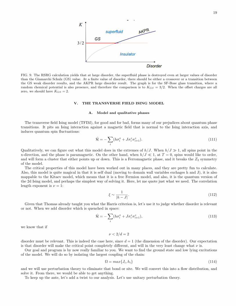
What do I mean by Jn with n ∈ clusters? We need to add the inverse bonds that make up the SF cluster - the oneswe decimated using the cluster formation step, which led to the formation of the cluster. We did this, and the resultwas non-universal. Without going into details, we obtain that when disorder is larger than some crossover value, theLttinger parameter at the transition we calculate is larger than 3/2 (in this case, since we have particle hole symmetry,the proper thing to say is that K > 2 = Kc for the SF-Mott glass transition). This is summarized in Fig. 9. This hasbecome controversial - how come weak disorder and large disorder are so different? This is still debated, but recentevidence from Thomas Vojta’s group is supportive of this prediction10.

19

FIG. 9. The RSRG calculation yields that at large disorder, the superfluid phase is destroyed even at larger values of disorderthan the Giamarchi Schulz (GS) value. At a finite value of disorder, there should be either a crossover or a transition betweenthe GS weak disorder results, and the AKPR large disorder result. The graph is for the SF-Bose glass transition, where arandom chemical potential is also presence, and therefore the comparison is to KGS = 3/2. When the offset charges are allzero, we should have KGS = 2.

V. THE TRANSVERSE FIELD ISING MODEL

A. Model and qualitative phases

The transverse field Ising model (TFIM), for good and for bad, forms many of our prejudices about quantum phasetransitions. It pits an Ising interaction against a magnetic field that is normal to the Ising interaction axis, andinduces quantum spin fluctuations:

H = −∑

i

(hσxi + Jσzi σzi+1). (111)

Qualitatively, we can figure out what this model does in the extremes of h/J . When h/J ≫ 1, all spins point in thex-direction, and the phase is paramagnetic. On the other hand, when h/J ≪ 1, at T = 0, spins would like to order,and will form a cluster that either points up or down. This is a Ferromagnetic phase, and it breaks the Z2 symmetryof the model.

The critical properties of this model have been worked out in many places, and they are pretty fun to calculate.Also, this model is quite magical in that it is self dual (moving to domain wall variables exchages h and J), it is alsomappable to the Kitaev model, which means that it is a free Fermion model, and also, it is the quantum version ofthe 2d Ising model, and perhaps the simplest way of solving it. Here, let me quote just what we need. The correlationlength exponent is ν = 1:

ξ ∼ 1

|h− J | . (112)

Given that Thomas already taught you what the Harris criterion is, let’s use it to judge whether disorder is relevantor not. When we add disorder which is quenched in space:

H = −∑

i

(hσxi + Jσzi σzi+1), (113)

we know that if

ν < 2/d = 2

disorder must be relevant. This is indeed the case here, since d = 1 (the dimension of the disorder). Our expectationis that disorder will make the critical point completely different, and will in the very least change what ν is.

Our goal and program is by now really familiar to you. We want to find the ground state and low lying excitationsof the model. We will do so by isolating the largest coupling of the chain:

Ω = maxJi, hi (114)

and we will use perturbation theory to eliminate that bond or site. We will convert this into a flow distribution, andsolve it. From there, we would be able to get anything.

To keep up the ante, let’s add a twist to our analysis. Let’s use unitary perturbation theory.

20

B. Unitary perturbation theory

Something that I learned during grad school which I found really useful, is how to do perturbation theory usingunitary transformation, rather than in terms of wave functions11. What’s the idea? Split your Hamiltonian to:

H = H0 + V. (115)

with V small compared to H0 in some sense. Now, we would like to find a transformation U = eiS for which:

eiSHe−iS = H0 + O(V 2) + EV . (116)

with EV a shift in energy which commutes with everything. We can then also try to cancel higher powers of V .Let’s find an S order by order that cancel the remnants of V . To first order:

eiSHe−iS = H0 + V + i[S, H0] + . . . (117)

Now it is obvious what we would like to do. Look for:

V = −i[S, H0] (118)

If you manage to do this, you’re in business! S will be of order V , and then you could read off corrections to theHamiltonian from the 2nd order of the transformed Hamiltonian. Continuing Eq. (117):

. . . i[S, V ]− 1

2S2H0 −

1

2H0S

2 + SH0S. (119)

In the end of the day, we hope to eliminate the non commuting pieces in the hamiltonian. We can then trivially

diagonalize it, and obtain a wavefunction,∣

∣

∣Ψ⟩

to get to a true eigenstate of the original problem, we just need to

undo the unitaries. Or:

eiSHe−iS∣

∣

∣Ψ⟩

= E∣

∣

∣Ψ⟩

→ He−iS∣

∣

∣Ψ⟩

= Ee−iS∣

∣

∣Ψ⟩

(120)

and we see that e−iS∣

∣

∣Ψ⟩

is an eignestate.

Turns out that one can use this method generically for diagonalizaing finite matrices, as well as it serves a basis fora field theoretic RG method coined ’Wegners flow equations’, on which there is a nice book by Stefan Kehrein, whois a pioneer of the method. The upshot of my exposure to ’flow equations’ is that S is vary often [H0, V ]. This isindeed the case in the TFIM.

Let us now derive the unitaries for h and J decimations of the TFIM. Maybe it is simpler to start with a large h.So choose:

H0 = −h1σx1 (121)

In this case we would like to freeze site 1 in the +x direction. We don’t need to decide on that though, and let’s justfind th unitaries. the main perturbation we would like to avoid is connection to neighbors:

V = −J01σz0σz1 − J12σz1σz2 . (122)

In order to eliminate the first order couplings to spin 0, S must satisfy equation (118); thus we first choose

Sa = − J012h1

σz0σy1 −

J122h1

σy1σz2 (123)

which yields the following terms in the effective Hamiltonian:

Heff =

. . .− J01J12h1

σz0σx1σ

z2 − h0J01

h1σy0σ

y1 − h2J12

h1σy1σ

y2 + . . .

(124)

The σyσy interaction appears as a correction to the Hamiltonian which does not commute with H0; site 1 is stillcoupled to adjacent sites by a second order interaction. By going to the next order, the Hamiltonian is restored toits original form. To get rid of it, we perform another transformation using

Sb = −h0J012h21

σy0σz1 −

h2J122h21

σz1σy2 . (125)

21

iS2

−h1σ1x−h−1σ−1

x σ0x−h0

σ−1y σ0

y σ1yσ0

y

h 0

01 1 −J h−10h 0

−1−J h

−h1σ1x−h−1σ−1

x σ0x−h0

σ−1z σ1

z

01J =O 2(1/Ω )2(1/Ω )

iS1

σ0z σ1

zσ−1z σ0

z −J01

−h−1σ−1x −h1σ1

xσ0x−h0

effH =e He

−10h 0

01

−10J =O

effH =e He−iS 1

−iS 2

−J J

−10−J

FIG. 10. Site decimation. Spin 0 is almost frozen in the x-direction due to the strong magnetic field h0. Quantum fluctuationscreate a second nearest neighbor effective interaction between sites -1 and 1. This interaction is weaker than any of J

−10, J01, h0.

The effective Hamiltonian now includes

Heff = . . .− J−10σz−1σ

z0 − h0σx0

−J02σz0σx1σz2 − h2σx2 − J23σz2σz3 + . . . ,

−h1σx1 ,(126)

from which we see that in the low-energy subspace of H0, the effective exchange between spins 0 and 2 is given by

J02 =J01J12h1

. (127)

Since h1 is the strongest coupling energy in the chain, the resulting effective bond obeys

J02 ≪ h0, J01, J12, (128)

where the sharpness of the inequality is because we assume strong randomness. We can now partially diagonalizeHeff by writing

|H >= | →>1 |G(1) >

|G >= e−iSae−iSb |H >,(129)

where σx1 | →1>= | →1> and |G(1) > involves only the spins other than 1. We are left with a renormalized spin-chain

with the spin at site 1 eliminated, and with an effective interaction J02σz0σ

z2 between spin 0 and spin 2. [Note that

we could also keep the high energy sector that involves | ←1>; the effective Hamiltonian and state of the rest of the

chain would differ from those of the low energy sector because of the presence of σx(1) in Heff of Eq. 126.]

The analog of the above results for the case where an exchange interaction, e.g. H0 = −J12σz1σz2 , is eliminated is

22

−h1σ1xσ0

x−h0

iS1iS2 −iS 1 −iS 2H =e e He eeff

σ−1z σ0

z−10−J −J

12σ1

z σ2z

−J12

σ1z σ2

zσ−1z σ0

z

h h 0 1

J01

h h 0 1

J01

σ1y σ01

xy0

σ = −

σ0z σ ∼11

z

−J01

σ0z σ1

z

−10−J

FIG. 11. Bond decimation. Sites 0 and 1 are frozen into one cluster by the strong Ising interaction, J01. Quantum fluctuationsproduce an effective magnetic field, h01 = h0h1

J01, which flips the composite spin cluster. This field is weaker than any of

h0, h1, J01.

(Fig. 11)

H0 = −J12σz1σz2V = −h1σx1 − h2σx2

Sa = h1

2J12σy1σ

z2 + h2

2J12σz1σ

y2

Sb = −h0J012J2

12

σy1σz0 − h3J23

2J212

σz3σy2 .

(130)

This could be obtained by using the duality described in Ref. 12, or by direct computation. The ground state ofH0 = −J12σz1σz2 is doubly degenerate with spins 1 and 2 either in the state | ↑(12)>= | ↑1> | ↑2> or in the state

| ↓(12)>= | ↓1> | ↓2>. Therefore in the ground state of H0 = σz1σz2 spin 1 and 2 form a ferromagnetic cluster, which

we denote as (12). We can define cluster operators, σz(12) and σx(12), that operate on the spin cluster (12) in the

following way:

σz1 ⇒ σz(12)

σz2 ⇒ σz(12)

−σy1σy2 ⇒ σx(12)

(131)

in terms of which

Heff − H0 =

. . .− h0σx0 − J0(12)σz0σz(12) + h(12)σx(12)σ

z1σ

z2

−J(12)3σz(12)σz3 − h3σx3 + . . . ,

(132)

with

h(12) =h1h2J12

(133)

being the effective transverse field on the new cluster (12) that has replaced the pair of spins 1 and 2 that now only

appear separately in the high energy term in H0. Again, since J12 is the strongest energy, and strong randomness isassumed, the effective transverse field obeys:

h12 ≪ h1, h2, J12. (134)

The amazing thing in this process is that we didn’t need to decide what the state we are intereseted in. Werenormalized the Hamiltonian as a whole!

23

C. Flow Equations and solution

Given the RG rules are products, it is clear we should define logarithmic variables:

β = lnΩ

hand ζ = ln

Ω

J. (135)

With these, the RG rules are precise sum rules:

βeff = βL + βR (136)

for a J decimation, and

ζeff = ζL + ζR (137)

for an h decimation.We don’t need to derive the RG flow equations anew. They are essentially identical to the Random-Heisenberg

flow, except that the probability in front of the convolution rule for J’s belongs to the h decimation, and vice versa.Denoting P (β) and R(ζ) the distributions for field and bond variables, we get:

dP (β)dΓ = ∂P (β)

∂β +R(0)∫

dβℓ∫

dβrP (βℓ)P (βr)δ(β − βℓ − βr) + P (β) · (P (0)−R(0))dR(ζ)dΓ = ∂R(ζ)

∂ζ + P (0)∫

dζℓ∫

dζrR(ζℓ)R(ζr)δ(ζ − ζℓ − ζr) +R(ζ) · (R(0)− P (0))(138)

Two things to note. First, unlike the Heisenberg model, we now do have terms that correct for normalization. The±(R0 −P0) terms that are last in both equations just rescale the distribution which they multiply, to make sure that

probability remains constant. Second, There is a subtle difference relative to the random boson equations - no ζ ∂f∂ζ ,

as opposed to Eq. (88). This subtle difference is what reflects the fact that the random bosons RG rules do not leadto infinite randomnes.

What are the fixed point distributions going to be? You can guess it - simple exponents. Again, let’s plug in anexponenetial ansatz:

P (β) = be−bβ , and R(ζ) = ge−gζ . (139)

where b and g are both functions of Γ. Plugging these into the flow equations (138) immediately reduces to the flowequation:

db

dΓ=dg

dΓ= −b · g (140)

Almost the same as random bosons, if we replace f with b. Solving these is a bit easier, since the flow equations areself dual. We note that the difference of the two paramaters is constant, and therefore:

d

dΓ(b− g) = 0→ b = g + 2δ (141)

where δ is going to serve as the tuning parameter of the FM-PM transition. Plugging this back in, we get:

dg

dΓ= −g(2δ + g). (142)

This equation can be directly integrated, and we obtain:

g = −δ + δ cot δΓ, and b = +δ + δ coth δΓ. (143)

This is pretty much it! Next, consequences. All of this was worked out by Daniel Fisher in his 1995 killer paper, 12.

D. Critical properties

We obtained the family of universal distributions as a function of a single parameter - δ. Just as we had it for therandom bosons, when δ = 0 we have a critical point. We can see this since then b = g → 1

Γ , which results in the same

24

ditribution as the random singletfixed point. But, what is δ in terms of initial distributions? As it turns out, and asyou can verify from the parameters b and g,

δ =ln J − lnh

√

var(ln J) + var(lnh)(144)

So δ > 0 implies J > h, and a ferromagnetic phase, and δ < 0 is the paramagnetic phase. Now we essentially haveeverything. What are the universal physical properties we can quickly get?

(1) First, as for the Heisenberg model, let’s get the density as a function of energy scale. Every time we lower theenergy scale, we have probability P (0)dΓ to have an h-decimation, which removes a single site, and R(0)dΓ probabilityto form a cluster out of two site, which also removes a single site. Together, their effect on the density is:

dn = −n · (b+ g)dΓ = −ndΓ2δ coth(δΓ). (145)

Integrated, this gives:

n =n0δ

2

sinh2 δΓ(146)

(2) How about correlation exponent? We said at first, that disorder must be important due to Harris criterion. Inthe clean case, ν = 1 < 2/d = 2. Do we satisfy the Harris criterion now? Let’s see. What determines the correlationlength? It is the length scale where it becomes clear that the chain is going to one phase or the other. Looking at thedistribution functions, it should be where the coth piece stops being important. This happens when Γ ∼ 1/|δ|.

Near criticality, the density-energy relationship is the same as that for the random singlet phase [as letting δ → 0shows in Eq. (146)]. So the length in which this crossover occurs is:

ℓ ∼ Γ2CO ∼

1

|δ|2 (147)

But this is exactly

ν = 2 (148)

as the Harris criterion dictates.(3) Here is a rather crucial fact that makes the TFIM near criticality into a Griffiths phase. What is the dynamical

critical exponent z (E ∼ ℓ−z)?At criticallity we have infinite randomness, so z → ∞, and we have the infinite randomness scaling. But off

criticality, if we look back at eq. (146), we should be able to read off the relationship between the lengthscale ofexcitations, ℓ, and their energy, by saying ℓ ∼ 1/n. We are looking for the scaling at large lengths, and therefore needto look at large Γ. we then have:

ℓ ∼ 1/n ∼ e2|δ|Γ = e2|δ| lnΩ1E ∼ E−2|δ| (149)

This is looking more like regular energy-length scaling, and we read off z:

z =1

2|δ| (150)

This energy-length scaling is the consequence of having extended deffects of the opposite phase in both the para-magnetic phase, as well as the ferromagnetic phase. Otherwise, the phase would have been gapped. The probabilityof these defects diminishes as one moves away from the critical point. This is reflected in z becoming more and morenormal as |δ| grows.

(4) An interesting thing I won’t derive is the correlations. Daniel Fisher calculated in his 95 paper that:

〈σznσzn+x〉 ∼1

x2−φ(151)

with φ = 1+√5

2 , which is the golden ratio. So the golden ratio pops up here as well.

25

E. Hilbert-glass transition in the TFIM

In the last few lines of this note I can add that the TFIM has played a strong role in our thinking of many-bodylocalization (MBL) like transitions. The MBL transition is a finite temperature transition from a disordered electronicsystem having no conductance at all, to having a finite conductance. It has no thermodynamic signatures otherwise.This transition is, therefore, between two classes of eigenstates of the system - localized, and delocalized.

The fact that we can carry out the RSRG in the TFIM without determining the state until the very end, and notnecessarily choose the ground state, means that the entire spectrum exhibits the FM-PM transition when δ = 0 - notjust the ground state. At finite temperatures, there are no signatures in the thermodynamics for this fact. Phasetransitions in any case are not allowed at 1d, finite temperature. The dynamics, though, will show that transition.

What are the dynamical signatures? On the FM side, each eigenstate has an inifinte cluster where all spins pointin the z-direction. Since most eigenstates are not ground states, there are going to be a lot of misalligned bonds inthe typical state. But the z-magnetization pattern is not going to fluctuate. So:

Ct =∑

n

〈n|σzi (0)σzi (t) |n〉 (152)

(with n being a state index, and the sum runs on the entire spectrum) is going to have a finite value in the δ > 0 FMside, and will average to 0 at the paramagnetic side.

We speculate that this is the generic picture for dynamical phase transitions of the kind MBL belongs to. Becuaseit is the eigenstates at arbitrary energy responsible for this, it is a transition in the Hilbert space, and we named itthe Hilbert glass transition13.

1 S. K. Ma, C. Dasgupta, and C. K. Hu, Phys. Rev. Lett. 43, 1434 (1979).2 C. Dasgupta and S. K. Ma, Phys. Rev. B 22, 1305 (1980).3 D. S. Fisher, Phys. Rev. B 50, 3799 (1994).4 L. C. Tippie and W. G. Clark, Phys. Rev. B 23, 5846 (1981).5 L. C. Tippie and W. G. Clark 23, 5854 (1981).6 E. Altman, Y. Kafri, A. Polkovnikov, and G. Refael, Physical Review Letters 93, 150402 (Oct. 2004), arXiv:cond-

mat/0402177.7 E. Altman, Y. Kafri, A. Polkovnikov, and G. Refael, Physical Review Letters 100, 170402 (May 2008), arXiv:0711.2070 [cond-

mat.dis-nn].8 E. Altman, Y. Kafri, A. Polkovnikov, and G. Refael, Phys. Rev. B 81, 174528 (May 2010), arXiv:0909.4096 [cond-mat.dis-

nn].9 E. Orignac, T. Giamarchi, and P. Le Doussal, Physical Review Letters 83, 2378 (Sep. 1999), arXiv:cond-mat/9903340.

10 F. Hrahsheh and T. Vojta, Physical Review Letters 109, 265303 (Dec. 2012), arXiv:1210.4807 [cond-mat.dis-nn].11 G. Refael and D. S. Fisher, Phys. Rev. B 70, 064409 (Aug. 2004), arXiv:cond-mat/0308176.12 D. S. Fisher, Phys. Rev. B 51, 6411 (1995).13 D. Pekker, G. Refael, E. Altman, E. Demler, and V. Oganesyan, ArXiv e-prints(Jul. 2013), arXiv:1307.3253 [cond-mat.str-el].