real-time acoustic identification of invasive wood-boring beetles
TRANSCRIPT

Real-time Acoustic Identification of Invasive Wood-boring
Beetles
James Schofield
Submitted for the degree of Doctor of Philosophy
University of York
Department of Electronics
July 2011

Abstract
Wood-boring beetles are a cause of significant economic and environmental cost across
the world. A number of species which are not currently found in the United King-
dom are constantly at risk of being accidentally imported due to the volume of global
trade in trees and timber. The species which are of particular concern are the Asian
Longhorn (Anoplophora glabripennis), Citrus Longhorn (A. chinensis) and Emerald Ash
Borer (Agrilus planipennis). The Food and Environment Research Agency’s plant health
inspectors currently manually inspect high risk material at the point of import. The de-
velopment of methods which will enable them to increase the probability of detection of
infestation in imported material are therefore highly sought after. This thesis describes
research into improving acoustic larvae detection and species identification methods, and
the development of a real-time system incorporating them.
The detection algorithm is based upon fractal dimension analysis and has been shown
to outperform previously used short-time energy based detection. This is the first time
such a detection method has been applied to the analysis of insect sourced sounds. The
species identification method combines a time domain feature extraction technique based
upon the relational tree representation of discrete waveforms and classification using arti-
ficial neural networks. Classification between two species, A. glabripennis and H. bajulus,
can be performed with 92% accuracy using Multilayer Perceptron and 96.5% accuracy
using Linear Vector Quantisation networks. Classification between three species can be
performed with 88.8% accuracy using LVQ.
A real-time hand-held PC based system incorporating these methods has been devel-
oped and supplied to FERA for further testing. This system uses a combination of dual
piezo-electric based USB connected sensors and custom written software which can be
used to analyse live recordings of larvae in real-time or use previously recorded data.
1

Contents
Abstract 1
List of figures 5
List of tables 7
Acknowledgements 11
1 Introduction 12
1.1 Governmental Organisations . . . . . . . . . . . . . . . . . . . . . . . . . . . 13
1.2 Novel Work . . . . . . . . . . . . . . . . . . . . . . . . . . . . . . . . . . . . 16
1.3 Thesis Structure . . . . . . . . . . . . . . . . . . . . . . . . . . . . . . . . . 16
2 Invasive Non-Native Species 20
2.1 Invasive Species . . . . . . . . . . . . . . . . . . . . . . . . . . . . . . . . . . 20
2.2 Wood-boring beetles and the Threat to Trees in the United Kingdom . . . . 28
2.3 Pathways and Vectors for Invasive Beetle Species . . . . . . . . . . . . . . . 30
2.4 Economic Impact . . . . . . . . . . . . . . . . . . . . . . . . . . . . . . . . . 32
2.5 Environmental Impact . . . . . . . . . . . . . . . . . . . . . . . . . . . . . . 32
2.6 Prevention, Detection, Monitoring and Control . . . . . . . . . . . . . . . . 33
2.7 Outbreak Case Studies . . . . . . . . . . . . . . . . . . . . . . . . . . . . . . 38
2.8 Summary . . . . . . . . . . . . . . . . . . . . . . . . . . . . . . . . . . . . . 40
3 Insect Acoustics 41
3.1 Sound Waves and Transmission . . . . . . . . . . . . . . . . . . . . . . . . . 41
3.2 Sound Transmission in Wood . . . . . . . . . . . . . . . . . . . . . . . . . . 43
3.3 Insects and Acoustics . . . . . . . . . . . . . . . . . . . . . . . . . . . . . . . 45
3.4 Wood Boring Beetles and Acoustics . . . . . . . . . . . . . . . . . . . . . . 48
2

Contents
3.5 Sounds produced by Larvae . . . . . . . . . . . . . . . . . . . . . . . . . . . 50
3.6 Anoplophora chinensis (Citrus Long-Horned Beetle) . . . . . . . . . . . . . 55
3.7 Anoplophora glabripennis (Asian Long-Horned Beetle) . . . . . . . . . . . . 57
3.8 Agrilus planipennis (Emerald Ash-Borer) . . . . . . . . . . . . . . . . . . . 59
3.9 Summary . . . . . . . . . . . . . . . . . . . . . . . . . . . . . . . . . . . . . 60
4 Acoustic Monitoring and Automated Detection 62
4.1 Acoustic Monitoring . . . . . . . . . . . . . . . . . . . . . . . . . . . . . . . 62
4.2 Automated Detection . . . . . . . . . . . . . . . . . . . . . . . . . . . . . . 68
4.3 Dual Sensor . . . . . . . . . . . . . . . . . . . . . . . . . . . . . . . . . . . . 85
4.4 Summary . . . . . . . . . . . . . . . . . . . . . . . . . . . . . . . . . . . . . 85
5 Species Identification 87
5.1 Feature extraction . . . . . . . . . . . . . . . . . . . . . . . . . . . . . . . . 87
5.2 Relational Trees . . . . . . . . . . . . . . . . . . . . . . . . . . . . . . . . . 97
5.3 Classification . . . . . . . . . . . . . . . . . . . . . . . . . . . . . . . . . . . 102
5.4 Summary . . . . . . . . . . . . . . . . . . . . . . . . . . . . . . . . . . . . . 120
6 System Implementation 121
6.1 Requirements and Overview . . . . . . . . . . . . . . . . . . . . . . . . . . . 121
6.2 Recording Equipment and Methods . . . . . . . . . . . . . . . . . . . . . . . 124
6.3 Hardware Implementation . . . . . . . . . . . . . . . . . . . . . . . . . . . . 126
6.4 Software Implementation . . . . . . . . . . . . . . . . . . . . . . . . . . . . . 130
6.5 Complete System . . . . . . . . . . . . . . . . . . . . . . . . . . . . . . . . . 137
6.6 Summary . . . . . . . . . . . . . . . . . . . . . . . . . . . . . . . . . . . . . 138
7 Conclusions and Further Work 140
7.1 Conclusions . . . . . . . . . . . . . . . . . . . . . . . . . . . . . . . . . . . . 140
7.2 Evaluation of the adopted system . . . . . . . . . . . . . . . . . . . . . . . . 141
7.3 Further Work . . . . . . . . . . . . . . . . . . . . . . . . . . . . . . . . . . . 143
Appendix 145
A Publication List 145
B Fractal Dimension C# Code 146
3

Contents
C Additional Classification Results 148
D Recordings made during this project 153
E Recordings made by others 154
References 155
4
List of Figures
1.1 Relationship between relevant organisations and departments . . . . . . . . 13
1.2 The stages of an identification system with chapter labels . . . . . . . . . . 17
2.1 Invasive Non-Native Species - Causes, Pathways and Vectors . . . . . . . . 21
2.2 Travel from the UK in 2009 . . . . . . . . . . . . . . . . . . . . . . . . . . . 24
2.3 Travel to the UK in 2009 . . . . . . . . . . . . . . . . . . . . . . . . . . . . 25
2.4 Value of Imports to the United Kingdom in 2010(Office for National Statis-
tics, 2011) . . . . . . . . . . . . . . . . . . . . . . . . . . . . . . . . . . . . . 26
2.5 Value of Exports from the United Kingdom in 2010(Office for National
Statistics, 2011) . . . . . . . . . . . . . . . . . . . . . . . . . . . . . . . . . . 26
2.6 Imports of Live Trees and Plants to the United Kingdom (2009) . . . . . . 30
2.7 Imports of Wood to the United Kingdom (2009) . . . . . . . . . . . . . . . 31
2.8 Exports of Live Trees and Plants from the United Kingdom (2009) . . . . . 31
2.9 Exports of Wood from the United Kingdom (2009) . . . . . . . . . . . . . . 31
3.1 Sound transmission . . . . . . . . . . . . . . . . . . . . . . . . . . . . . . . . 42
3.2 Cross-section of a tree . . . . . . . . . . . . . . . . . . . . . . . . . . . . . . 44
3.3 Categories of insect produced sounds . . . . . . . . . . . . . . . . . . . . . . 46
3.4 The Lifecycle of a Wood-Boring Beetle . . . . . . . . . . . . . . . . . . . . . 49
3.5 Diagram of cerambycid head (Adapted from (Duffy, 1968)) . . . . . . . . . 51
3.6 An Anoplophora glabripennis bite . . . . . . . . . . . . . . . . . . . . . . . . 52
3.7 An Agrilus planipennis bite . . . . . . . . . . . . . . . . . . . . . . . . . . . 52
3.8 Anoplophora chinensis adult (Image provided by FERA, used with permis-
sion) . . . . . . . . . . . . . . . . . . . . . . . . . . . . . . . . . . . . . . . . 55
3.9 A. glabripennis adult (Image provided by FERA, used with permission) . . 57
3.10 Agrilus planipennis adult . . . . . . . . . . . . . . . . . . . . . . . . . . . . 59
5
List of Figures
4.1 Acoustic Monitoring and Detection Process . . . . . . . . . . . . . . . . . . 63
4.2 Sensor Coupling Experiment . . . . . . . . . . . . . . . . . . . . . . . . . . 66
4.3 Voltage at sensor vs input frequency . . . . . . . . . . . . . . . . . . . . . . 67
4.4 Voltage at sensor vs distance from source . . . . . . . . . . . . . . . . . . . 68
4.5 Bite with energy overlayed . . . . . . . . . . . . . . . . . . . . . . . . . . . . 71
4.6 Sierpinski Triangle . . . . . . . . . . . . . . . . . . . . . . . . . . . . . . . . 73
4.7 Koch Curve . . . . . . . . . . . . . . . . . . . . . . . . . . . . . . . . . . . . 74
4.8 Anoplophora glabripennis bite with Fractal Dimension overlayed (Frame
size 200 samples) . . . . . . . . . . . . . . . . . . . . . . . . . . . . . . . . . 77
4.9 Fractal Distance and Energy Distance vs Signal to Noise Ratio (Embedded
Bites, Frame Size 200 Samples) . . . . . . . . . . . . . . . . . . . . . . . . . 79
4.10 Fractal Distance and Energy Distance vs Signal to Noise Ratio (Embedded
Sine Wave, Frame Size 200 Samples) . . . . . . . . . . . . . . . . . . . . . . 79
4.11 Fractal Distance vs Frame Size Multiple for embedded sine wave at 10dB . 80
4.12 Fractal Distance vs Frame Size Multiple for embedded bites at 10dB . . . . 81
4.13 Detection of random noise, ambient noise and bites . . . . . . . . . . . . . 82
4.14 Event Expansion . . . . . . . . . . . . . . . . . . . . . . . . . . . . . . . . . 84
4.15 Activity of unknown larva over 20 hour period . . . . . . . . . . . . . . . . 84
5.1 Distribution of FD Values . . . . . . . . . . . . . . . . . . . . . . . . . . . . 91
5.2 Example of waveform epochs (D1,S1) and (D2,S2) . . . . . . . . . . . . . . 92
5.3 Example codebook . . . . . . . . . . . . . . . . . . . . . . . . . . . . . . . . 93
5.4 Two waveforms with identical TDSC encoding . . . . . . . . . . . . . . . . 95
5.5 Complete (left) binary tree and incomplete (right) binary trees . . . . . . . 97
5.6 Example waveform . . . . . . . . . . . . . . . . . . . . . . . . . . . . . . . . 98
5.7 Example relational tree (Depth 3) . . . . . . . . . . . . . . . . . . . . . . . 99
5.8 Normalised relational tree (Depth 3) . . . . . . . . . . . . . . . . . . . . . . 100
5.9 Example relational tree with numbered nodes . . . . . . . . . . . . . . . . . 101
5.10 Perceptron with single input . . . . . . . . . . . . . . . . . . . . . . . . . . 104
5.11 Perceptron with vector input . . . . . . . . . . . . . . . . . . . . . . . . . . 105
5.12 Linear Separability . . . . . . . . . . . . . . . . . . . . . . . . . . . . . . . 105
5.13 Multiple Layer Perceptron Network . . . . . . . . . . . . . . . . . . . . . . . 106
5.14 Self Organising Map . . . . . . . . . . . . . . . . . . . . . . . . . . . . . . . 107
5.15 LVQ Network . . . . . . . . . . . . . . . . . . . . . . . . . . . . . . . . . . . 109
6

List of Figures
5.16 Effect of quantization on A. glabripennis vs H. bajulus classification . . . . 115
5.17 Effect of quantization on A. glabripennis vs H. bajulus vs Noise classification 115
6.1 Components of a Detection System . . . . . . . . . . . . . . . . . . . . . . . 122
6.2 Side view of encased sensor . . . . . . . . . . . . . . . . . . . . . . . . . . . 125
6.3 Sensor attached using a tree strap . . . . . . . . . . . . . . . . . . . . . . . 126
6.4 Sensor attached using rubber bands . . . . . . . . . . . . . . . . . . . . . . 127
6.5 USB Dual Sensor Design . . . . . . . . . . . . . . . . . . . . . . . . . . . . 129
6.6 Software Overview . . . . . . . . . . . . . . . . . . . . . . . . . . . . . . . . 131
6.7 Detection Process . . . . . . . . . . . . . . . . . . . . . . . . . . . . . . . . 133
6.8 Bite Identification Process . . . . . . . . . . . . . . . . . . . . . . . . . . . 135
6.9 Threads . . . . . . . . . . . . . . . . . . . . . . . . . . . . . . . . . . . . . . 136
6.10 Complete System . . . . . . . . . . . . . . . . . . . . . . . . . . . . . . . . . 139
7

List of Tables
2.1 Causes of invasions (Adapted from (Wittenberg and Cock, 2001) and (Burgiel
et al., 2006)) . . . . . . . . . . . . . . . . . . . . . . . . . . . . . . . . . . . 23
2.2 Common Pathways For INNS . . . . . . . . . . . . . . . . . . . . . . . . . . 24
2.3 Economic Costs of INNS (Adapted from (Emerton and Howard, 2008)) . . 27
2.4 Beetles which are a threat to trees in the United Kingdom . . . . . . . . . . 29
2.5 Wood-boring beetles present in the EPPO A1 & A2 lists (EPPO, 2005) . . 29
2.6 FERA Plant Material Categories. Adapted from (FERA, 2008). . . . . . . 33
3.1 Frequencies of insect produced sounds . . . . . . . . . . . . . . . . . . . . . 48
3.2 Anoplophora chinensis outbreaks in Europe . . . . . . . . . . . . . . . . . . 56
3.3 Basic Dimensions of Anoplophora chinensis . . . . . . . . . . . . . . . . . . 56
3.4 A. glabripennis outbreaks outside Asia . . . . . . . . . . . . . . . . . . . . . 58
3.5 Basic Morphology of A. glabripennis . . . . . . . . . . . . . . . . . . . . . . 58
3.6 Basic Morphology of Agrilus planipennis . . . . . . . . . . . . . . . . . . . . 60
4.1 Summary of sensors used to detect insects in plants and timber . . . . . . . 65
4.2 Table of sensors tested . . . . . . . . . . . . . . . . . . . . . . . . . . . . . 66
4.3 The dimensions of common geometric shapes . . . . . . . . . . . . . . . . . 72
5.1 Feature extraction methods used in the analysis of beetle larvae sounds . . 88
5.2 A. glabripennis TDSC shape values . . . . . . . . . . . . . . . . . . . . . . . 96
5.3 H. bajulus TDSC shape values . . . . . . . . . . . . . . . . . . . . . . . . . 96
5.4 Noise event TDSC shape values . . . . . . . . . . . . . . . . . . . . . . . . . 96
5.5 Serialised Relational Tree Values . . . . . . . . . . . . . . . . . . . . . . . . 102
5.6 Applications of ANN to animal sound classification . . . . . . . . . . . . . . 102
5.7 Applications of ANN to time domain feature classification . . . . . . . . . 103
5.8 Anoplophora glabripennis recordings . . . . . . . . . . . . . . . . . . . . . . 111
8

List of Tables
5.9 A. glabripennis vs. H. bajulus confusion matrix (Tree depth 4) . . . . . . . 113
5.10 A. glabripennis vs. H. bajulus (Tree depth 2) . . . . . . . . . . . . . . . . . 113
5.11 A. glabripennis vs. H. bajulus (Tree depth 3) . . . . . . . . . . . . . . . . . 113
5.12 A. glabripennis vs. H. bajulus (Tree depth 5) . . . . . . . . . . . . . . . . . 113
5.13 A. glabripennis vs. H. bajulus (Tree depth 6) . . . . . . . . . . . . . . . . . 114
5.14 A. glabripennis vs. H. bajulus Summary . . . . . . . . . . . . . . . . . . . . 114
5.15 A. glabripennis vs. H. bajulus LVQ Results (20 first layer nodes) . . . . . . 116
5.16 A. glabripennis vs. H. bajulus LVQ Results (30 first layer nodes) . . . . . . 116
5.17 A. glabripennis vs. H. bajulus LVQ Results (40 first layer nodes) . . . . . . 116
5.18 A. glabripennis vs. H. bajulus LVQ Results (50 first layer nodes) . . . . . . 117
5.19 A. glabripennis vs. H. bajulus vs. Noise LVQ Results (20 first layer nodes) . 117
5.20 A. glabripennis vs. H. bajulus vs. Noise LVQ Results (30 first layer nodes) . 117
5.21 A. glabripennis vs. H. bajulus vs. Noise LVQ Results (40 first layer nodes) . 118
5.22 A. glabripennis vs. H. bajulus vs. Noise LVQ Results (50 first layer nodes) . 118
5.23 Bite vs. Noise MLP Results . . . . . . . . . . . . . . . . . . . . . . . . . . 118
5.24 Bite vs. Noise LVQ Results (20 first layer nodes) . . . . . . . . . . . . . . . 118
5.25 Bite vs. Noise LVQ Results (30 first layer nodes) . . . . . . . . . . . . . . . 119
5.26 Bite vs. Noise LVQ Results (40 first layer nodes) . . . . . . . . . . . . . . . 119
5.28 A. glabripennis vs. A. planipennis vs. H. bajulus LVQ Results (50 first
layer nodes) . . . . . . . . . . . . . . . . . . . . . . . . . . . . . . . . . . . . 119
5.27 Bite vs. Noise LVQ Results (50 first layer nodes) . . . . . . . . . . . . . . . 120
6.1 Hand-held System Requirements . . . . . . . . . . . . . . . . . . . . . . . . 123
6.2 Data-logging System Requirements . . . . . . . . . . . . . . . . . . . . . . 123
6.3 Selection of AC ’97 Analogue performance characteristics . . . . . . . . . . 127
6.4 Example Frame Results Table . . . . . . . . . . . . . . . . . . . . . . . . . 134
6.5 Events List Truth Table . . . . . . . . . . . . . . . . . . . . . . . . . . . . . 135
C.1 A. glabripennis vs. H. bajulus MLP, Depth 4, Quantization 200 levels . . . 148
C.2 A. glabripennis vs. H. bajulus MLP, Depth 4, Quantization 100 levels . . . 148
C.3 A. glabripennis vs. H. bajulus MLP, Depth 4, Quantization 50 levels . . . . 148
C.4 A. glabripennis vs. H. bajulus MLP, Depth 4, Quantization 20 levels . . . . 149
C.5 A. glabripennis vs. H. bajulus MLP, Depth 4, Quantization 10 levels . . . . 149
C.6 A. glabripennis vs. H. bajulus MLP, Depth 4, Quantization 4 levels . . . . 149
9

List of Tables
C.7 A. glabripennis vs. H. bajulus MLP, Depth 4, Quantization 2 levels . . . . 149
C.8 A. glabripennis vs. H. bajulus MLP, Depth 4, Quantization 1 level . . . . . 149
C.9 A. glabripennis vs. H. bajulus vs. Noise MLP, Depth 4, Quantization 200
levels . . . . . . . . . . . . . . . . . . . . . . . . . . . . . . . . . . . . . . . . 150
C.10 A. glabripennis vs. H. bajulus vs. Noise MLP, Depth 4, Quantization 100
levels . . . . . . . . . . . . . . . . . . . . . . . . . . . . . . . . . . . . . . . . 150
C.11 A. glabripennis vs. H. bajulus vs. Noise MLP, Depth 4, Quantization 50
levels . . . . . . . . . . . . . . . . . . . . . . . . . . . . . . . . . . . . . . . . 150
C.12 A. glabripennis vs. H. bajulus vs. Noise MLP, Depth 4, Quantization 20
levels . . . . . . . . . . . . . . . . . . . . . . . . . . . . . . . . . . . . . . . . 151
C.13 A. glabripennis vs. H. bajulus vs. Noise MLP, Depth 4, Quantization 10
levels . . . . . . . . . . . . . . . . . . . . . . . . . . . . . . . . . . . . . . . . 151
C.14 A. glabripennis vs. H. bajulus vs. Noise MLP, Depth 4, Quantization 4 levels151
C.15 A. glabripennis vs. H. bajulus vs. Noise MLP, Depth 4, Quantization 2 levels151
C.16 A. glabripennis vs. H. bajulus vs. Noise MLP, Depth 4, Quantization 1 level 152
D.1 List of recordings made during this project . . . . . . . . . . . . . . . . . . 153
E.1 List of recordings made by others . . . . . . . . . . . . . . . . . . . . . . . . 154
10

Acknowledgements
I would like to thank DEFRA for providing the funding for this research and their
staff at FERA, York for providing assistance on many occasions. I am also grateful to
the following organisations who provided either recordings of larvae or the opportunity to
record infestations:
• Dipartimento Di Agronomia Ambientale e Produzioni Vegetali, Universita Degli
Studi Die Padova, Italy.
• Fondazione Minoprio, Italy.
• National Plant Protection Organization, Netherlands
I would like to thank my supervisor Dr. Chesmore for all of his assistance and guidance
throughout this research, and my wife Claire for her unwavering support throughout my
time spent studying. Finally I would like to thank my family and friends who have
supported me over the past few years.
11

Chapter 1
Introduction
In an age of mass international and intercontinental travel and wide-ranging global trade,
animals, plants and other organisms are frequently transported between nations both in-
tentionally and accidentally. Without suitable border control procedures the risk of acci-
dentally introducing a non-native species into the United Kingdom is high. Some species,
if introduced in this manner would become invasive; that is to say they would become
established, potentially at the expense of other native species, and may pose a significant
threat to the economy and environment.
Two commonly known examples of invasive species in the UK are the Grey Squirrel
(Sciurus carolinensis) and the Japanese Knotweed (Fallopia japonica). The former causes
environmental damage to trees by stripping bark whilst the latter causes economic damage
as it weakens infrastructure such as roads and drains (Rayden and Savill, 2004), (Williams
et al., 2010).
In the United Kingdom, the Department for Environment, Food and Rural Affairs
(DEFRA) is the government department which has overall responsibility over the mitiga-
tion of such threats. One area of particular concern to DEFRA is the movement of plant
material between countries. Imported living plants may harbour pathogens such as Phy-
tophthora ramorum, which causes ’sudden oak death’, and Phytophthora kernoviae which
damages beech and rhododendron (FERA, 2011b), (FERA, 2011c). The threat is by no
means limited to living plants; sawn timber, trees and even wooden packaging material
may contain pests such as the Citrus Longhorn Beetle which will be discussed in detail in
chapters 2 and 3 (FERA, 2010), (Haack et al., 2010).
12

1.1 Governmental Organisations
The European Commission produces EU wide legislation regarding the import and
export of plant material in the form of its Plant Health Directive (2000/29/EC) (European
Commission, 2000). This includes lists of species for which import into the EU is forbidden
or restricted, requiring specific measures such as kiln drying to have been undertaken prior
to import. A statement on the opening page of the directive provides a justification for the
measures: “Plant production yields are consistently reduced through the effects of harmful
organisms. The protection of plants against such organisms is absolutely necessary not
only to avoid reduced yields but also to increase agricultural productivity” (European
Commission, 2000).
1.1 Governmental Organisations
Figure 1.1: Relationship between relevant organisations and departments
A number of governmental organisations have responsibilities regarding invasive species
and the import of plant material. As described in the previous section, DEFRA has overall
13

1.1 Governmental Organisations
responsibility; however this is delegated to an executive agency, The Food and Environ-
ment Research Agency (FERA). The FERA website states that “Fera is responsible, on
behalf of Defra, for implementing the plant health Regulations in England and Wales (on
behalf of the Welsh Assembly Government). The Scottish Government is responsible for
implementation in Scotland. Separate but similar arrangements apply in Northern Ire-
land.” (FERA, 2011d).
A department of FERA, the Plant Health and Seeds Inspectorate (PHSI) has offices
across the U.K. and is the body which is responsible for the inspection of plant mate-
rial. This inspection is primarily performed manually and involves time-consuming visual
inspection and destructive sampling of material. PHSI inspectors detect plant pests not
only at points of entry to the U.K such as sea and airports but also at nurseries to issue
plant passports for export and to monitor plants during post import growth.
The Forestry Commission is the organisation responsible for the management and pro-
tection of Britain’s forests and woodland (Forestry Commission, 2011b). It has its own
Plant Health Service (PHS) which cooperatives with PSHI to form the UK Plant Health
Service. The Forestry Commission states the following: “The Forestry Commissions Plant
Health Service (PHS) operates throughout Great Britain to prevent harmful pests enter-
ing GB and the European Union from overseas, and to eradicate or contain any that do
become established.” (Forestry Commission, 2011a).
An intergovernmental organisation, the European and Mediterranean Plant Protection
Organization (EPPO), produces pan-European standards, publications and recommenda-
tions regarding plant health issues. Its stated objectives are “to protect plants, to develop
international strategies against the introduction and spread of dangerous pests and to
promote safe and effective control methods” (EPPO, 2011). EPPO maintains two lists
of species which it recommends that its members regulate; the A1 list, which contains
species not present within the EPPO region, and the A2 list, which contains species al-
ready present in the region (EPPO, 2010).
14

1.1 Governmental Organisations
1.1.1 Relationship to DEFRA project PH0191
A previous DEFRA funded project, PH0191, with which the author had no involvement,
is the predecessor to the current project. Part of the previous project involved feasibility
study into the possible use of an automated acoustic system for the detection and recog-
nition of insect pests. The overall aim of this project was to “to consider the feasibility
of utilising novel acoustic detection technologies in the development of a tool for onsite
detection and recognition of quarantined pests” (Farr, 2007).
The research proved that the automated acoustic detection and identification of beetle
larvae is possible (to a limited extent). Classification of bites between two species, Hy-
lotrupes bajulus and Prionus coriarius was performed to 97.8% accuracy (Farr, 2007) and
prototype (non-realtime) acoustic larvae detection and identification system was produced
during this project.
1.1.2 DEFRA Project PH0419
The research described in this thesis was undertaken as part of DEFRA Project PH0419
which was established as a result of the previous project. The proposal for this project
states the following:
“The purpose of this project is to aid the work of the Plant Health and
Seeds Inspectors (PHSI) and Forestry Commission (FC) inspectors by improv-
ing their ablity to detect a range of statutory/quarantine pests using the acous-
tic methods initially investigated in a previous Plant Health Division funded
project PH0191, which established proof of principle” (DEFRA, 2007)
In order to achieve this the proposal sets out two specific tasks:
1. Refine the techniques which were developed in the earlier project (PH0191).
This will include final consideration of optimal sensor selection and refinement of the
species identification stage of the process.
2. Produce two systems for use by PHSI and FC inspectors
a) The first system will perform real-time determination of the presence of quaran-
tine species, and where required, an initial identification.
15

1.2 Novel Work
b) The second system will be capable of stand-alone operation and will act through
a datalogging system, which can be used during transport of suspect material as well
as at the point of import or at in-land points of destination.
At each stage of the system (sensors, audio capture, detection and identification) the
approaches untertaken in the previous project will be investigated. Their suitability, with
refinements where necessary, will be considered along with alternative approaches for
implementation in the final real-time detection and identification system(s).
1.2 Novel Work
The novel work presented in this thesis is outlined below:
• The use of fractal dimension analysis as a method for the detection of larval activity
sounds. This method outperforms short time energy detection for low amplitude
events.
• The use of relational trees as a feature extraction technique to encode larval acoustic
activity.
• The combination of relational tree features and artificial neural networks to acous-
tically identify wood-boring beetle larvae by species. Classification rates of 99%
between two species and 90.4% between three species has been achieved.
• The development and implementation of a system capable of automated real-time
beetle larvae detection and identification.
1.3 Thesis Structure
The chapters in this thesis are arranged to follow the stages of an automated acoustic de-
tection and classification system. This begins by looking at the problem, invasive species,
which are the reason for the development of the system. The sound source, beetle larvae,
is then introduced in chapter 3. The automated detection process, which might be con-
sidered by some as classification between beetle species and noise, is covered in a separate
16

1.3 Thesis Structure
chapter to species identification. This is primarily because the methods use for bite de-
tection are unrelated to those used for species identification due to the nature of the two
tasks in this situation. Results are given within the relevant chapters rather than being
listed separately. The system implementation chapter covers all stages of the detection
and identification process. Figure 1.2 is intended to provide an overview of the relationship
between chapters.
Chapter 2 introduces the concept of invasive species and covers their threat to both
Figure 1.2: The stages of an identification system with chapter labels
the economy and the environment. It provides justification for this research by describing
the scale of the problem posted by outbreaks of invasive beetle species and the limitations
of the methods which are currently employed to detect their accidental introduction into
the United Kingdom. Containment and eradication methods which have been used by
governments to deal with outbreaks and infestations in other countries is also covered.
The chapter concludes with case studies on two recent outbreaks of invasive wood-boring
beetle species in the United States and Italy.
Chapter 3 covers the relationship between wood, insects and acoustics. The chapter
begins by describing the process of acoustic transmission within materials and wood in
particular, and looks at factors which may affect the transmission and ability to detect
sounds at the surface of the wood. Sounds which may be sourced from the wood itself
rather than any insects contained within are also considered.
17

1.3 Thesis Structure
Section 3.3 describes the categories of sounds which can be produced by insects along
with the reasons for their production and the physical mechanisms which are used. The
chapter then goes on to cover wood-boring beetle species in particular and the sounds
which they produce during each stage of their life-cycles in relation to their suitability
for use in an acoustic detection system. Sounds produced as a by-product of the feeding
of larvae are detailed and factors which may affect their production are considered. The
chapter concludes with case studies on two beetle species, the Asian Longhorn and Citrus
Longhorn, which are of particular interest to this research.
Chapter 4 covers the methods used to detect the sound associated with the feeding of
larvae from the surrounding noise. The chapter begins by considering the two categories
of insect sound recording methods, substrate and airborne. The selection of optimum
sensors for use in recording is then covered.
The computational methods which are currently used for acoustic event detection are
then investigated before a new technique based upon Fractal Dimension analysis is intro-
duced. A performance comparison between this method and Short Time Energy Detection
is provided. Finally, the use of a secondary sensor for the reduction of false positive events
is covered in addition to results for varied detection threshold levels.
Chapter 5 covers the methods used to identify the species of detected larval events.
The chapter begins by detailing methods which have been used by others to detect and
identify insects by their acoustic emissions.
A new identification method using relational tree structures in combination with an
Artificial Neural Network (ANN) classifier is then introduced. Results are then provided
for the classification between a number of species of beetle and between beetle and noise
where a number of properties of the feature extraction method are varied.
Chapter 6 describes the implementation of the detection system as a whole. The chapter
begins by considering the specified and implied requirements which DEFRA and PHSI
have for the system. The methods and equipment used for acoustic recording of larvae
18

1.3 Thesis Structure
before the development of the automated system are then described. The hardware im-
plementation is covered in section 6.3 and the use of dual channel USB attached sensors is
described and justified. Section 6.4 covers the software implementation and aims to pro-
vide an overview of the system’s capabilities in terms of input and output options. The
relationship between the detection and identification stages in the software is described
in addition to an overview of the threads which are used to allow the software to perform
real-time analysis. The chapter concludes with a summary of the system which was de-
livered to PHSI to testing.
Chapter 7 provides conclusions on the research undertaken as part of this project. It also
considers further work which could be undertaken as a result this research and in other
areas which would allow the system described in this thesis to be developed further.
19

Chapter 2
Invasive Non-Native Species
This chapter serves as a justification for the research and is intended to give the reader
an understanding of the scale of the problem which is faced by DEFRA and other related
government agencies, and therefore the reasons for interest in the development of a sys-
tem to assist in combating the threat. It introduces concept of invasive non-native species
(INNS) along with their pathways, vectors, and impact on economy and environment.
The specific threat of wood-boring beetles to trees in the United Kingdom is dis-
cussed in section 2.2 which includes lists of high risk species. This section also includes
estimates for the potential environmental and economic impact of outbreaks of invasive
beetle species. Section 2.6 describes the methods which are currently used to prevent
INNS from being imported in addition to control and eradication techniques which are
used in pest outbreak situations.
The chapter concludes with case studies of outbreaks of two of the species of interest
to this project, the Asian Longhorn and Citrus Longhorn Beetles, including a summary
of the costs incurred and governmental responses.
2.1 Invasive Species
The term ‘Invasive Species’ has multiple definitions; in some cases it is used to describe
only non-native species, in others it includes native species which are considered to have
a negative impact on their surroundings. Similarly, the term is often used to describe any
non-native species which is widespread, regardless of it’s impact (Binggeli, 1994), (Colautti
20

2.1 Invasive Species
and MacIsaac, 2004).
In the United Kingdom, an Invasive Non-Native Species (INNS) is defined by DEFRA
as “any non-native animal or plant that has the ability to spread causing damage to the
environment, the economy, our health and the way we live” (DEFRA, 2011); this term
will be used for the remainder of this thesis. This chapter will also use the terms Pathway
and Vector; the relationship between these along with examples are shown in Figure 2.1.
Figure 2.1: Invasive Non-Native Species - Causes, Pathways and Vectors
INNS pose a potential threat on a huge scale; it is estimated that over 11,000 non-
native species have entered Europe (DAISIE, 2009) and approximately ten new non-native
taxa become established across Europe each year (Hulme et al., 2009). Additionally, an
estimated 21.4% of vascular plant species in Britain and Ireland are non-native (Vitousek
et al., 1996).
2.1.1 Causes of invasions
Causes of invasions are either natural, accidental or intentional. Accidental and inten-
tional invasions occur when human activity provides a suitable pathway and vector to
carry the INNS. Pathways and Vectors are discussed in more detail in Sections 2.1.2 and
2.1.3 respectively. Accidental introductions are the by-product of the movement of per-
sons or goods between different geographical areas. These may include, for example, the
21

2.1 Invasive Species
importing of a non-native species to a zoo only for it to later escape and become invasive.
The unintentional importing of a non-native species within internationally traded goods
would also fall into this category. Accidental causes are generally related to human desire
for internationally available goods or services.
Non-native species are sometimes introduced intentionally for economic or environmen-
tal reasons. For example, the American Mink (Mustela vison) was intentionally introduced
to Europe in the 1920’s for use in fur farming (Birnbaum, 2006). Escapes and intentional
releases have resulted in the species becoming invasive (Bonesi and Palazon, 2007).
In Toronto, Canada, the Norway Maple (Acer platanoides) was introduced into public
spaces as a replacement for North American Elm (Ulmus americana). It subsequently
spread across the country and is now considered an invasive species (Foster and Sanberg,
2004). Another tree species, Saltcedar (Tamarix spp.), a perennial plant native to Eurasia,
has become an invasive species in North America since it’s introduction as an ornamental
in the 19th century (Dudley and DeLoach, 2004). It is considered an undesirable species
as it increases salt levels in the soil and displaces native vegetation (APHIS, 2005b). A leaf
beetle, Diorhabda elongata, has successfully been introduced to some sites as a biological
control agent (Dudley et al., 2006).
Stoats (Mustela erminea) were introduced to New Zealand in the 1880s to control the
rabbit population (also an introduced species). However, the stoats predated on a native
bird, the Brown Kiwi (Apteryx mantelli) to near extinction and are now considered inva-
sive (King et al., 2007).
A list of common causes of invasions, categorised by whether they involve intentional
or accidental introduction, is provided in Table 2.1.
2.1.2 Pathways
A pathway is the route from source to destination through which a species travels. These
pathways may be natural or non-natural; common pathways for INNS are listed in Table
2.2.
Natural pathways are those which occur without human interference, for example cur-
22

2.1 Invasive Species
Intentional Introductions Accidental Introductions
Direct Indirect
Agriculture Pets released into wild Agricultural produce
Forestry Zoo escapes Nursery plants
Soil Improvements Garden escapes Cut Flowers
Food resources Farming Timber
Ornamental Plants Research facilities Seeds
Hunting Aquaculture Soil
Biological Control Machinery and equipment
International aid Packaging material
Fishery Cargo
Conservation Ballast Water
Sentimental Reasons Ballast soil
International planes
Hull fouling
Luggage
Table 2.1: Causes of invasions (Adapted from (Wittenberg and Cock, 2001) and (Burgiel
et al., 2006))
rents in rivers, seas or the atmosphere (Ruiz and Carlton, 2003). The gulf stream is an
example of a natural pathway as it has introduced tropical plants to the Isles of Scilly
(Lousley, 1971). As natural pathways exist without the need for human interference there
is little that can be done to prevent the introduction of INNS through them.
The majority of pathways for invasive species are non-natural, that is to say they are
pathways created intentionally or unintentionally as a result of human activity. Generally
speaking non-natural pathways are the result of travel, transport, trade or tourism and
can consist of waterways, air-routes, railways or roads.
a) Travel and Tourism
International travel and tourism creates many potential pathways for INNS. In 1981, 11.5
million visits were made to the UK and 19 million visits to foreign countries were made by
UK residents (Office for National Statistics, 2011). By 2009, these figures had increased
23

2.1 Invasive Species
Pathways
Natural Non-Natural
Atmospheric Currents Trade Related. e.g. Container ship routes
Oceanic Currents Transport Related. e.g. Motorway corridors
Rivers Tourism Related. e.g. Flight paths
Land Migration Travel Related
Table 2.2: Common Pathways For INNS
to 29.9 million visits to the UK, and 58.6 million visits from the UK; increases of 260% and
196% respectively. Figures 2.2 and 2.3 show the breakdown of sources and destinations
for these visits.
Europe (73.9%)
Other Countries (14.2%)
North America (11.9%)
Figure 2.2: Travel from the UK in 2009
b) Trade and Transport
The economy of the United Kingdom is heavily reliant on international trade. The move-
ment of internationally traded goods provides a significant pathway for invasive species.
Figures 2.4 and 2.5 show the major sources and destinations of the United Kingdom’s
imports and exports. The major pathway for accidental invasion is internationally traded
cargo (Ruiz and Carlton, 2003). In 2001, 2.2 million tonnes of freight was handled by UK
airports and 566 million tonnes was handed by UK ports.
24

2.1 Invasive Species
Europe (78.4%)
Other Countries (15.4%)
North America (6.2%)
Figure 2.3: Travel to the UK in 2009
2.1.3 Vectors
A vector is the physical means by which an INNS is transported. A simple example being
a person carrying a species from one location to another. Several vectors of INNS are
related to international shipping. Ballast water, for example, is a significant vector for
marine borne invasive species (Carlton and Geller, 1993); this is water which is stored
within tanks on a ship to maintain its stability. This water is taken from the port from
which the ship originates and can introduce non native species to the ship’s destination if
the ballast water is released. INNS can also be vectored by their physical attachment to
the hulls of ships. The Zebra mussel (Dreissena polymorphia) was introduced to Ireland
in the mid 1990s in this manner (Minchin et al., 2003).
The most significant shipping related vector is the movement of goods between coun-
tries. Several wood boring insects have been introduced by this vector. The European
woodwasp (Sirex noctilio) was first discovered in New York in 2004, and in Ontario,
Canada in 2005; most likely having been vectored by imported wood. (de Groot et al.,
2006).
Whinam et al. conducted a study into the risk of expeditioners vectoring non-native
species to subantarctic islands. Instrument cases and Velcro on clothing were identified
25

2.1 Invasive Species
Irish Republic Italy Belgium Norway France Netherlands China United States Germany Others0
10
20
30
40
50
60
70
80
90
100
110
120
130
140
Pou
nds
Ste
rling
(B
illio
ns)
Country
Value of United Kingdom Imports by Country (2010)
Figure 2.4: Value of Imports to the United Kingdom in 2010(Office for National Statis-
tics, 2011)
China Italy Spain Belgium Irish Republic France Netherlands Germany United States Others0
10
20
30
40
50
60
70
80
90
100
Pou
nds
Ste
rling
(B
illio
ns)
Country
Value of United Kingdom Exports by Country (2010)
Figure 2.5: Value of Exports from the United Kingdom in 2010(Office for National
Statistics, 2011)
as high risk vectors. On an expedition in 2002, 44% of cargo items were found to be
contaminated and 90 species were collected from the clothing of the 64 expeditioners
(Whinam et al., 2005).
2.1.4 Economic Costs
These can be significant economic costs associated with the introduction of an invasive
species. The economic costs of invasive species can be broken down into management
costs, production losses and other costs. Management costs are those associated with the
prevention, control or eradication of the INNS. This may include labour, research fund-
26

2.1 Invasive Species
ing, equipment and publicity. Table 2.3 shows the areas of economic cost in addition to
examples.
Direct Costs Indirect Costs
Management Costs Opportunity Costs Opportunity Costs
Prevention, Eradication,
Monitoring and Contain-
ment.
Production Losses e.g. de-
creased productivity
Impact on other sectors
e.g. reduced employment
Labour, research funding,
equipment and publicity
Increased disease damage. Reduced availability and
higher prices of vectors
Restoration Costs Water shortage Infrastructure damage
Table 2.3: Economic Costs of INNS (Adapted from (Emerton and Howard, 2008))
2.1.5 Environmental Impact
There are several ways in which an INNS can have a negative environmental impact. An
INNS may successfully compete with a native species for resources, as the Grey squir-
rel (Sciurus carolinensis) does in the United Kingdom. INNS can also be responsible
for lowering the biodiversity in their new habitat, for example the previously mentioned
Saltcedar (see Section 2.1.1). Other INNS may attack species which are not used to having
predators as has happened in North America where the Emerald Ash Borer is estimated
to have destroyed more than 20 million trees in 10 years (Cappaert et al., 2005).
2.1.6 Other Issues
INNS can have a negative impact on human health, for example Smallpox (Variola virus)
could be considered an INNS as it was introduced to the Americas by the Spanish in the
1500s (Glynn and Glynn, 2004). Some INNS are responsible for causing injuries and al-
lergies, such as the Brown tree snake (Boiga irregularis) and the Gypsy moth (Lymantria
dispar). The Oak Processionary moth (Thaumetopoea processionea) causes lepidopterism,
a form of dertmatitis, in humans when they come in contact with the hairs of its larvae
(Maier et al., 2003). Other species are themselves vectors of human diseases, for exam-
ple the Raccoon Dog (Nyctereutes procyonoides) which is a vector for rabies (Pyek and
Richardson, 2010).
27

2.2 Wood-boring beetles and the Threat to Trees in the United Kingdom
2.1.7 Species Examples
2.1.7.1 Japanese Knotweed
The Japanese Knotweed (Fallopia japonica) is plant native to Japan, China and Korea
which is classified as an invasive species in both the United Kingdom and other countries.
It was introduced to the United Kingdom intentionally in the nineteenth century to be
used in gardens (Williams et al., 2010). The plant causes environmental damage as it
competes for resources with other plants. In the USA, Japanese Knotweed stem density
has been shown to have a negative correlation with native plant species density, indicating
that the knotweed can displace native species (Urgenson et al., 2009). It can cause damage
to infrastructure such as tarmac and drains, and costs an estimated £5 million each year
across the road network of Great Britain (Williams et al., 2010). The total costs of
Japanese Knotweed to the British economy have been estimated as over £165 million
annually (Williams et al., 2010).
2.1.7.2 Grey Squirrel
The Grey squirrel (Sciurus carolinensis) is a mammal native to North America. It was
introduced to “various locations in Britain between 1876 and the 1920s” (Mayle et al.,
2007). It strips bark, causing damage to a wide range of trees in the United Kingdom
(Rayden and Savill, 2004).
There are also significant economic costs associated with its presence; a Forestry
Commission document estimates that in Great Britain, Grey squirrel damage to beech,
sycamore and oak will cause losses of around £10 million due to reduced crop value
(Forestry Commission, 2006).
2.2 Wood-boring beetles and the Threat to Trees in the
United Kingdom
The specific beetles which are considered a threat to the United Kingdom can be deter-
mined from various lists which are produced by relevant governmental organisations. The
Forestry Commission maintains lists of pests which currently threaten trees in the United
Kingdom and of threats not yet present (Forestry Commission, 2011c). The list includes
28

2.2 Wood-boring beetles and the Threat to Trees in the United Kingdom
the five species of beetle which are shown in Table 2.4 below.
Species Present in the UK
Emerald ash borer (Agrilus planipennis) No
Citrus longhorn beetle (Anoplophora chinensis) No
Great spruce bark beetle (Dendroctonus micans) Yes
Oak pinhole borer (Platypus cylindrus) Yes
Eight-toothed European spruce bark beetle (Ips typographus) No
Table 2.4: Beetles which are a threat to trees in the United Kingdom
Species EPPO List
City Longhorn Beetle (Aeolesthes sarta) A2
Emerald Ash Borer (Agrilus planipennis) A2
Citrus Longhorn Beetle (Anoplophora chinensis) A2
Asian Longhorn Beetle (Anoplophora glabripennis) A1
Ambrosia Beetle (Megaplatypus mutatus) A2
Round-headed apple tree borer (Saperda candida) A1
Fine-horned Spruce Borer (Tetropium gracilicorne) A2
Altai Longhorn Beetle (Xylotrechus altaicus) A2
Will Longhorn Beetle (Xylotrechus namanganensis) A2
Table 2.5: Wood-boring beetles present in the EPPO A1 & A2 lists (EPPO, 2005)
Two species of beetle, the Asian Longhorned beetle (Anoplophora glabripennis) and
the Khapra beetle (Trogoderma granarium), are listed amongst the 100 worst invasive
species (Lowe et al., 2004) and the losses caused in the US by 43 alien insects between
1906 and 1991 have been estimated at over $92.5 billion (OTA, 1993). The cost of the
invasion in the USA since 1996 of Asian Longhorned Beetle has been over $267 billion
and has required the removal of 30,000 trees (USDA, 2007). The presence of beetles on
this list and those produced by the Forestry Commission and EPPO show that invasive
beetle species are considered to be a significant threat in the United Kingdom, Europe
and worldwide.
29

2.3 Pathways and Vectors for Invasive Beetle Species
2.3 Pathways and Vectors for Invasive Beetle Species
As discussed in Section 2.1.2, a pathway is route through which an INNS is introduced
to a new area, whilst a vector is the physical means by which the INNS travels through
the pathway. The major vectors for wood-boring beetles are trees and wood products.
This project is primarily concerned with preventing the accidental invasion of alien beetle
species through the importing these vectors. In the four years up to 2006 almost 15 million
cubic metres of wood with an approximate value of £669 billion was either imported to
or exported from the United Kingdom (Forestry Commission, 2007).
Data from the Office for National Statistics shows that in 2009, over 5.7 billion items
in the category ‘Wood and articles of wood; wood charcoal’ were imported into the United
Kingdom (Office for National Statistics, 2011). The source countries for these imports
are shown in Figure 2.7. In the same time period over 297 million items in the category
‘Live trees and other plants; bulbs, roots and the like; cut flowers and ornamental foliage’
were imported. The source countries for these imports are shown in Figure 2.6. Figures
2.6 to 2.9 have been produced from data derived from the Office for National Statistics
(Office for National Statistics, 2011).
Figure 2.6: Imports of Live Trees and Plants to the United Kingdom (2009)
30

2.3 Pathways and Vectors for Invasive Beetle Species
Figure 2.7: Imports of Wood to the United Kingdom (2009)
Figure 2.8: Exports of Live Trees and Plants from the United Kingdom (2009)
Figure 2.9: Exports of Wood from the United Kingdom (2009)
31

2.4 Economic Impact
2.4 Economic Impact
The economic costs likely to be incurred due to an INNS have been discussed in Section
2.1.4. In this section the potential economic costs related to the introduction of invasive
beetle species will be considered in more detail.
The Centre for Agricultural Bioscience International (CABI) produced a report for
DEFRA, the Scottish government and the Welsh Assembly which provides estimates of
the economic costs of invasive species (Williams et al., 2010). The report estimates that
the INNS cost the United Kingdom £1.7 billion each year, of which £1 Billion is in the
agriculture and horticulture sector. It also states that the greatest INNS costs are inflicted
by plants.
The report also provides estimates which are specific to beetle species. Storage pests,
the majority of which are non-native, are estimated to cost £6.5 million per year to control.
A single species, the great bark spruce beetle ( Dendroctonus micans) causes damages to
forests and costs an estimated £32,000 per year in biological control and £130,840 per
year in loss of yield (Williams et al., 2010).
Estimates are also provided on the likely costs of potential outbreaks for species which
are not currently present. The report estimates that if the Asian Longhorn Beetle were to
become established in the United Kingdom it could cost up to £1.3 billion to eradicate,
based upon costs incurred in other countries. It estimates that if an infestation were left
uncontrolled, the cost to the forestry industry would over £400 million based upon costs
in the US (Williams et al., 2010).
2.5 Environmental Impact
The environmental impact of INNS can be difficult to quantify, particularly when trying to
estimate the potential impact of the introduction of a species. The CABI report described
in the previous section estimates that a single Asian Longhorn beetle infested tree could
result in the destruction of 78.5ha of forest in order to control its spread (Williams et al.,
2010).
32

2.6 Prevention, Detection, Monitoring and Control
Other estimates can be made by considering the environmental impact of beetle infes-
tations in other countries. The Emerald Ash Borer infestation in the US, for example, is
estimated to have destroyed more than 20 million trees in 10 years (Cappaert et al., 2005).
2.6 Prevention, Detection, Monitoring and Control
2.6.1 Prevention Methods
2.6.1.1 Legislation and Phytosanitary Certificates
Measures are routinely taken to prevent live larvae or adult beetles from being transported
between countries. In the U.K, FERA is responsible for plant health matters. It separates
imported plant material into three categories. These categories and their descriptions are
shown in Table 2.6.
Category Description
Prohibited “Poses such a serious risk that import is only permitted under author-
ity of a licence issued by FERA/WAG or the Forestry Commissioners.
Includes many species of rooted plants and trees from outside Europe.”
Controlled “Normally requires a phytosanitary certificate issued by the plant pro-
tection service of the exporting country. Includes those cuttings, rooted
plants and trees that are not prohibited, bulbs, most fruits, certain seeds
and some cut flowers.”
Unrestricted “Presents little or no risk and is not subject to routine plant health
controls. Includes nearly all flower seeds, some cut flowers and fruit and
most vegetables for eating (except potatoes).”
Table 2.6: FERA Plant Material Categories. Adapted from (FERA, 2008).
Since material in the ‘Prohibited’ category is largely prevented from being imported,
the most significant day to day risk is posed by imported material in the ‘Controlled’
category. As stated in Table 2.6, this material usually travels with a phytosanitory cer-
tificate which aims to prove that it has been inspected and meets the requirements for
entry. FERA states that a phytosanitory certificate is “a statement that the plants or
plant produce or products to which it relates have been officially inspected in the country
of origin (or country of despatch), comply with statutory requirements for entry into the
33

2.6 Prevention, Detection, Monitoring and Control
EC, are free from certain serious pests and diseases, and are substantially free from other
harmful organisms” (FERA, 2008).
2.6.1.2 Wood Treatment
Some sawn timber must be treated before it is allowed to be imported into the United
Kingdom; this may involve kiln drying, heat treatment and bark removal. The specific
requirements for the treatment of sawn timber are detailed in the Plant Health (Forestry)
Order 2005.
The International Plant Protection Convention (IPPC) has produced a standard for the
treatment of wood packaging material, “ISPM15 - Regulation of wood packaging material
in international trade” (IPPC, 2009). This requires wood packaging material to be heat
treated and stamped before export. The standard was incorporated into EU plant health
legislation through EC council directive 2004/102/EC (European Commission, 2004).
2.6.2 Detection Methods used in the UK
Any material in the ‘Controlled’ category are inspected at the point of entry to the UK
by plant health inspectors. Material in the ‘Unrestricted’ category may also be subject
to random inspection (FERA, 2008). These inspections include a physical check for pests
and diseases. For plants at risk of carrying invasive beetle species, the physical check
includes visual inspection and manual destructive sampling.
2.6.2.1 Visual Inspection
In some cases a larval infestation can be detected through visual inspection alone. An
inspector can look for visual indications of the possible presence of an infestation such
as ovi-position holes, exit holes or frass around holes and at the base of trees. Such in-
dications may not always be present or may be difficult to recognise; the risk of a false
negative result is therefore high. This is particularly relevant in the case of an infested
tree from which no adults have emerged. Another area of difficultly is in the inspection
of timber products and pallets which can contain larvae but are more difficult to inspect
than living trees since exit holes may be obscured and larvae may be located anywhere
within the product.
34

2.6 Prevention, Detection, Monitoring and Control
2.6.2.2 Manual Destructive Sampling
Manual destructive sampling is the method currently employed by Plant Health Inspectors
when investigating at risk plants entering the U.K. A proportion of samples are manually
cut into small pieces and a visual inspection for signs of larval inspection is carried out.
This is method is time consuming, expensive in terms of loss of commodity, and has a risk
of human-error. There are some circumstances where destructive sampling is not always
a viable option, for example where an individual high value plant is being transported.
2.6.3 Other Detection Methods
2.6.3.1 X Ray
Attempts have been made to detect wood-boring larvae with the use of X-Rays. In his
1940 paper, Fisher details the varying degrees of sucess in detection of a number of larvae
using this method (Fisher, 1940). The wood samples used varied in thickness from 3
16
inches (0.48cm) to 21
4inches (5.71cm). The equipment used and small wood sample sizes
required meant that this method could be of little use outside the laboratory environment.
X rays have been used numerous times to detect larvae inside grain (Schatzki et al.,
1993), (Keagy and Schatzki, 1991). In their 2004 paper, Karunakaran et al. show that
a combination of X ray and neural network based classification can be used to detect
Rhyzopertha dominica with 99% success (Karunakaran et al., 2004). It is highly unlikely
that such a technique could be adapted for the purpose of detecting larvae within wood
due to the lack of portability of equipment used and the physical size difference between
wheat kernels and standing trees. The author is not aware of any publications detailing
the successful detection of wood boring larvae in standing trees using X ray methods.
2.6.3.2 Sniffer Dogs
Sniffer dogs have been successfully used to detect a number of insects including Gypsy
moths (Lymantria dispar) (Wallner and Ellis, 1976), bed bugs (Cimex lectularius) (Pfi-
ester et al., 2008) and screwworms (Cochliomyia hominivorax ) (Welch, 1990).
Welch trained a German wirehaired pointer (Canis familiaris) to look for screwworms.
An overall success rate of 99.7% was achieved, with a success rate of 94.7% for screwworm
35

2.6 Prevention, Detection, Monitoring and Control
infested animals. 8 months of training was required before the dog was able to detect
screwworm pupae.
Pfiester et al. trained dogs to detect bed bugs and bed bug eggs. A 98% success rate
in locating live bed bugs in a hotel room environment was achieved.
Recently there have been attempts to detect Bark Beetles using sniffer dogs (Feicht,
2006). It is unclear to the author as to whether this research is still ongoing.
2.6.3.3 Acoustic Detection
It has been known for several decades that, in certain conditions, wood-boring larvae can
be detected acoustically. One of the earliest recorded methods of acoustic detection of lar-
vae in timber used a variety of microphones as the sensor (Colebrook, 1937). This method
required the wood under observation to be enclosed in a sound-proof container. Whilst no
automated detection or analysis was performed in this experiment it demonstrated that
larvae biting within timber does produce a detectable sound at the timber’s surface. A
similar approach was applied to listen for larvae in the timber of buildings (Schwarz et al.,
1935). This demonstrated that acoustic detection can be used to detect larvae in a noisy
environment.
Over the past 15 years interest in automated acoustic detection has grown and a num-
ber of methods have been investigated. These include the use of ultrasound (Fleming
et al., 2005), piezo-electric and bi-morph sensors (Farr, 2007) and accelerometers (Mankin
et al., 2004) in combination with various signal processing techniques to provide auto-
mated detection. Acoustic monitoring in general and automated detection using acoustics
will be discussed in greater detail Chapter 4.
2.6.4 Eradication and Control Methods
Although the ideal situation is to have detected and prevented any invasive species from
entering the country and therefore preventing any outbreaks, this is not always possible.
A number of eradication and control methods have been used on established outbreaks.
36

2.6 Prevention, Detection, Monitoring and Control
2.6.4.1 Host Destruction
As the title suggests this involves the destruction of host trees, usually limited to high
risk species over a defined area around an outbreak site. This method is expensive both
environmentally and economically not only due to the cost of removal but also the cost of
purchasing and planting replacement trees.
2.6.4.2 Biological and Microbial Control
There have been a small number of publications on the use of fungi to control beetle
populations. Higuchi et al. investigated the use of a fungus, Beauveria brongniartii, as
a control agent for yellow spotted longicorn beetle (Psacothea hilaris Pascoe) and deter-
mined through field trials on tangerine crops that it was capable of killing adult beetles
and preventing further infestation (Higuchi et al., 1997).
Hajek et al. conducted studies into the effectiveness of a number of species of fungi
against the Asian longhorned beetle (Hajek et al., 2007). Infection with Metarhizium
anisoplia F52 was found to cause adult female beetles to produce fewer eggs before their
death.
Herard et al. studied the egg parasitoid Aprostocetus anoplophorae as a potential bio-
logical control agent for Asian and Citrus Longhorn beetles (Herard et al., 2004), (Delvare
et al., 2004). The study concluded that the parasitoid has potential to be used as a control
agent for Citrus Longhorn but not Asian Longhorn beetles.
2.6.5 Outbreak Monitoring
2.6.5.1 Sentinel Trees
Sentinel trees are used in some infestation sites to help monitor the spread of the invading
species. Trees which are known hosts of the invader are placed around the infestation in
order to attract it to them as it spreads.
This technique was used to monitor the spread of Anoplophora chinensis in Lombardia,
Italy. Sentinel trees were placed within a buffer zone extending 1-2km from the infested
37

2.7 Outbreak Case Studies
area and visually inspected twice per year for signs of infestation (Maspero et al., 2007).
Field studies have shown that both sexes of Anoplophora glabripennis are highly at-
tracted to Acer pictum subsp. mono (Smith et al., 2009). A second species, sycamore
maple (A. pseudoplatanus) has been used as a sentinel tree during Anoplophora glabripen-
nis eradication efforts in Italy (Herard et al., 2009a).
2.6.5.2 Acoustic Monitoring
A detection system capable of automatically identifying beetle larvae could potentially
be used to assist in outbreak monitoring. Such a system could be combined with the
sentinel tree approach to more efficiently monitor the spread of the outbreak. The use of
a wireless sensor network combined with an automated acoustic detection system opens
up the possibility of a fully automated outbreak monitoring technique requiring little or
no human intervention.
2.7 Outbreak Case Studies
2.7.1 Anoplophora glabripennis outbreaks in the US
The Asian Longhorned beetle is indigenous to China and Southeast Asia. Over 40 species
of host tree have been identified (Yang et al., 1995), but the major hosts are Populus nigra,
Populus deltoides, Poplulus x canadensis, Populus dakhuanensis and Salix spp. (EPPO,
2004). The presence of an infestation weakens the host tree, and on leaving, adults pro-
duce large exit holes which may ooze sap (APHIS, 2005a). The Asian Longhorned beetle
is discussed in greater detail in Section 3.7 of Chapter 3.
Asian Longhorned beetle was first discovered in the US in 1996, in New York City
(Haack et al., 1997). Further outbreaks have since been discovered in Chicago, Illinois, in
1998 (Poland et al., 1998) and Jersey City, New Jersey, in 2002 (Haack, 2003).
U.S. Department of Agriculture (USDA) officials have determined that the vector of the
initial outbreak was solid wood packing material (SWPM) from China (APHIS, 2005a).
The initial response was to introduce a federal quarantine to regulate the movement of at
risk host material and to introduce an eradication program to rid the US of infested trees
38

2.7 Outbreak Case Studies
(Haack, 2003). The USDA believes that the most effective method of eradication is to cut
and chip or burn infested trees (APHIS, 2005a). Wang et al. conducted a study showing
that chipping is sufficient for killing nearly all larvae (Wang et al., 2000).
As of 2003, the infestations had required the removal of over 30,000 trees and cost
more than $269 million. Potential losses of over $41 billion were estimated should the
infestations spread beyond the initial three quarantined areas (APHIS, 2007).
2.7.2 Anoplophora chinensis outbreak in Lombardia, Italy
The Citrus Longhorned beetle is indigenous to China and Korea. The EU commission
considers 17 species to be the most significant hosts (FERA, 2010). These include Acer
spp. (maple), Salix spp. (willow) and Populus spp. (poplar). Citrus Longhorned bee-
tle causes damage in a very similar way to Asian Longhorned beetle. Infested trees are
left more susceptible to diseases and leaf damage can be caused by the feeding of adults
(FERA, 2010).
Citrus Longhorned beetle was first discovered in Lombardy, Italy in 2000 (Colombo
and Limonta, 2001). As of 2007, infestations had been identified in 30 municipalities
around Milan (Maspero et al., 2007). The European and Mediterranean Plant Protection
Organisation (EPPO) believes the vector for the infestations to be ornamental trees im-
ported from East Asia (Herard et al., 2009b).
The governmental response to the outbreak was to initiate eradication and monitoring
programmes. The monitoring relied heavily on the use of sentinel trees (as described in
Section 2.6.5.1) which were planted within a buffer zone around the outbreak area. The
buffer zone extended 1-2km outside the known infested area.
Between 2001 and June 2007, 3098 trees had been destroyed as part of the eradication
process (Maspero et al., 2007).
39

2.8 Summary
2.8 Summary
This chapter has introduced the concept of INNS and the related terms ‘Pathways’ and
‘Vectors’. The common causes of invasion, categorised into natural, accidental or inten-
tional have been discussed. The cost of invasive species with regards to their impact on the
environment and economy has been discussed. The increasing risk to the U.K of invasion
of invasive species in general due to its levels of international trade, transport and tourism
has been considered.
The risk posed by wood-boring beetle species has been described in detail and the
economic and environmental costs associated with infestations have been considered. An
overview of the different methods which have been used to prevent, detect, monitor and
control invasive beetle infestations has been given and the use of automated acoustic de-
tection as a preventative technique has been introduced.
Finally, case studies of outbreaks of two of the species of interest to this project
(Anoplophora glabripennis) and Anoplophora chinensis in the US and Italy have been
produced.
40

Chapter 3
Insect Acoustics
This chapter covers the combination of larvae and host tree as a sound source, beginning
by detailing how sound waves are transmitted through different materials and the proper-
ties which can affect transmission. Trees and timber as media for sound transmission and
as sound sources are then considered and the basic structure of trees is outlined.
The next area to be covered is the types of sound which are produced by insects and
the categories into which they are placed based upon the method by which they are pro-
duced and the purpose for their production.
The sound production of wood-boring beetles and in particular their larvae is then
explained in relation to the acoustic detection task; this includes looking at the relationship
between the behaviour and morphology of the larvae and the resulting sounds; and the
possible impact of a number of properties of the host. Finally, detailed descriptions of the
three beetle species which are of most interest to this research (Anoplophora glabripennis,
Anoplophora chinensis and Agrilus planipennis) are given.
3.1 Sound Waves and Transmission
Sound is simply the transmission of vibration through the particles of a material. The
principles remain the same whether the material may be solid, liquid, or gas. Sound is
transmitted, or propagated, through a material by the transfer of energy between the
particles that make up the material. The sound source causes particles to vibrate; this
in turn causes neighbouring particles to vibrate and so on. Each time this vibration is
41

3.1 Sound Waves and Transmission
passed on a small amount of energy is lost. The term used for the loss of energy through
transmission is attenuation.
Figure 3.1 gives a basic overview of sound transmission. The upper half of the figure
shows the sound wave’s impact on the pressure of particles as it progresses away from the
source. The darker bands represent high pressure and the lighter bands low pressure. The
lower half of the figure shows the perception of the sound received over a period of time
by the observer. The period of the sound wave, also known as the wavelength is the time
between successive periods of peak or minimum pressure.
Figure 3.1: Sound transmission
42

3.2 Sound Transmission in Wood
3.2 Sound Transmission in Wood
For the purposes of detecting wood-boring larvae, the sound source can be considered to
be the combination of larvae and host material (the tree, plant or wood). The physical
properties of the host material will affect both the ability to detect the presence of any
larvae, and the exact nature of sounds detected.
The composition of a material affects sound travelling through it in two significant
ways: attenuation and velocity. Attenuation is the rate at which energy is lost by the
sound wave as it passes through the material; velocity being the speed at which a wave
travels through the material. Density primarily affects the velocity of the wave, with sound
being transmitted faster in less dense materials. This is because a particle of lower mass
can be displaced further than a particle of greater mass given the same amount of force
exerted on it. The density of wood clearly varies between species but is also dependent on
other factors. In dried conditions, the density of Oak can be between 1 and 3 times that
of Canadian Pine and 5 times that of Balsa wood (simetric, 2009).
3.2.1 Factors influencing the acoustic properties of wood
Even after taking into account variations between difference species, the acoustic proper-
ties of wood can vary. Cut wood or packing materials are more likely to vary in moisture
content than standing trees; this can affect the both the attenuation and velocity of sound
within wood. As moisture content increases, wood density increases leading to a decrease
in sound velocity (Unterwieser and Schickhofer, 2011).
Another property to consider is the degree of decay; like moisture content this can
change the density of the wood. It does not occur evenly meaning that areas of very low
density may occur within in otherwise un-decayed wood. The level of decay can affect the
ease of attachment of sensors and the quality of acoustic coupling attained once sensors
are attached.
Figure 3.2 shows the cross-section of a tree trunk with different regions labelled. It
can be seen from this diagram that a tree is not a simple continous solid with unchanging
structure, but a complex one with several layers each with differing density and elasticity.
The layer in which a sound is produced may have a significant impact on how well it is
43

3.2 Sound Transmission in Wood
Figure 3.2: Cross-section of a tree
transmitted to the tree’s surface.
Finally, the grain within wood produces a variation in density meaning that the speed
of sound transmission is related to the angle of the wave to the grain (Ross, 1999). In the
case of live trees there is nothing that can be done to adjust the angle of the sensor with
respect to the grain, however in cut wood there may be advantages in placing sensors at
particular angles.
3.2.2 Wood Sourced Acoustic Emissions (AE)
In addition to transmitting sounds, in certain situations trees and wood may also be a
sound source. One cause of wood sourced AE is stress and fracture. As is the case with
other solid materials, as pressure is exerted on wood fibres they can break producing vibra-
tions which travel through the tree or timber. Several studies have used these emissions in
the stress testing of timber and as an indicator of decay (Raczkowski et al., 1999), (Antal,
2004), (Ayarkwa, 2010).
44

3.3 Insects and Acoustics
Some sounds are produced in standing trees but not in cut wood, by virtue of them
consisting of living material. An example of this is sound produced due to cavitation,
which is defined as “the formation of one or more pockets of gas (or cavities) in a liquid”
(Apfel, 1981). This process occurs within the fibres of trees as low sap pressure causes
xylem walls to break and become filled with air (Bucur, 2006). The emissions produced by
cavitation can be detected using ultra-sonic sensors at the surface of the wood (Borghetti
et al., 1989), (Raschi et al., 1989).
3.3 Insects and Acoustics
Insects produce a wide range of sounds for a variety of purposes and for no purpose at
all; these can be divided into two distinct categories. Incidental sounds are those pro-
duced as a by-product of some other action which the insect performs, such as feeding.
Non-incidental is used to categorise any sound intentionally produced, for example in com-
munication. Figure 3.3 shows most common insect sounds categorised by their type. For
non-incidental sounds the reason for producing the sound is given, for example to attract
a mate; for incidental sounds the action for which the sound is a by-product is given, for
example feeding.
Non-incidental sounds are most commonly produced for some form of communication
with other members of the same species, Cicadas, for example produce a sound to attract
others (Alexander and Moore, 1958). Communication sounds can be further categorised
by the situation in which they are produced. Ewing lists the known categories as: calling,
courtship, aggregation, aggression, copulation and disturbance (Ewing, 1984). Intention-
ally produced sounds are not limited to communication; recent studies have shown that
Tiger Moths (Bertholdia trigona) use non-incidental sounds for self preservation by dis-
rupting bat sonar (Corcoran et al., 2009).
The method of transmission of sounds by insects can be further categorised into two
groups, substrate and airborne. Substrate in this context means the material which an
insect is on or in, often a plant or tree as opposed to airborne in which sound is transmitted
without the use of a solid medium. The means of production of these sounds may involve
some form of physical interaction with the substrate such as striking. The means of sound
transmission has implications on the methods which are used to detect them; this will be
45

3.3 Insects and Acoustics
Figure 3.3: Categories of insect produced sounds
discussed in Chapter 4.
Sounds in both of these categories by be produced by a number of different physical
mechanisms. In his 1957 paper, Alexander produced five categories for the mechanisms
used by insects in sound production; these categories are summarised below (Alexander,
1957).
• Stridulation
This is where sound is produced as one body part is rubbed against another. An
example of this is species of Dung Beetle, Aphodius ater, which uses an organ on the
abdomen to produce stridulation (Hirschberger, 2001). Hirschberger hypothesises
that the sound produced is used by females to select mates since only the male of
the species regularly stridulates.
46

3.3 Insects and Acoustics
• Striking
This is the striking of a part of the insect’s body against the substrate or another
area of the body. Various different body parts are used depending on the insect
species; for example some male cockroaches use this mechanism by striking their
abdomen (Bell et al., 2007). The Death Watch Beetle (Xestobium rufovillosum)
performs a similar action by striking the head (Birch and Keenlyside, 1991).
• Vibration
The vibration of a body part, such as the wings, can produce airborne sounds. All
flying insects produce incidental sounds as the oscillation in their wings is transmit-
ted to the surrounding air. The frequencies produced by the wings of most insects
falls within the range 50Hz to 2kHz (Price, 1984); bees, for example, beat their
wings at around 190Hz (Chapman, 1998). Butterflies and moths tend to beat their
wings at a slower rate, producing sounds at frequencies as low as 8Hz (Corben, 1983).
• Tymbal vibration
Some insects have drum-like membranes called tymbals which can be vibrated. A
tymbal is a highly specialised body part which exists only for sound production;
it’s surface either has a number of ribs or is smooth and produces a clicking sound
when caused to buckle by an associated muscle (Shaw and Carlson, 1979). Ex-
amples of insects which produced sounds using this mechanism include Moths and
Cicada (Fullard and Heller, 1990), (Simmons and Young, 1978). Sounds produced
by Cicadas using tymbals are in the range 4 - 7kHz (Gullan and Cranston, 2010),
(Bennet-Clark, 1997), (Young and Bennet-Clark, 1995).
• Ejection of air or fluid
Hissing or whistling sounds are produced as air or fluid is forced out of the body. The
sound produced may be incidental, produced purely as a by-product rather than an
intentional sound; some grasshoppers for example eject a jet of liquid as a defence
mechanism (Hingston, 1927). In other insects sound is produced intentionally by
47

3.4 Wood Boring Beetles and Acoustics
this method; the Madagascar hissing cockroach (Gromphadorhina portentosa) is one
such example (Clark and Moore, 1995).
The range of frequencies which can be produced by different insects is wide, ranging
from the infrasonic, such as that of butterfly wing beating, to ultrasonic, such as the
stridulation of katydids (Corben, 1983), (F. Montrealegre-Z and Mason, 2006). Table 3.1
provides a summary of insect produced sounds and their frequency ranges.
Species Sound Type Frequency Reference
Butterflies Vibration 8 - 90 Hz (Corben, 1983)
Death Watch
Beetle
Striking ≈ 11Hz (White et al.,
1993)
Bees Vibration ≈ 190Hz (Chapman, 1998)
Tree Hoppers Striking ≈ 500Hz (Cocroft, 1999)
Cicadas Tymbal Vibration 4 - 7 kHz (Gullan and
Cranston, 2010),
(Bennet-Clark,
1997)
Grasshoppers Stridulation up to 30 kHz (von Helversen
and von Helver-
son, 1998),(van
Staaden and
Rmer, 1997)
Bush Crickets Stridulation up to 129 kHz (F. Montrealegre-
Z and Mason,
2006)
Table 3.1: Frequencies of insect produced sounds
3.4 Wood Boring Beetles and Acoustics
Before considering the types of sound that may be produced by wood-boring beetles the
lifecycles and behaviour of these insects should first be understood in order to determine
how best to detect them. Figure 3.4 shows the lifecycle of a wood-boring beetle.
48

3.4 Wood Boring Beetles and Acoustics
Figure 3.4: The Lifecycle of a Wood-Boring Beetle
The specifics of each of the stages within the insect’s lifecycle varies between and some-
times within species depending on external influences such as temperature. For example,
the length of time spent as an adult and the number of larval instars is known to vary
(Adachi, 1994). The Cottonwood Borer (Plectrodera scaltor), a pest which attacts the
roots of trees in the United States, is known to have at least five instars (Forschler and
Nordin, 1991). Larvae of the Asian Longhorn Beetle may pass through up to 14 instars
(Keena and Moore, 2010).
Like most insects, adult beetles produce detectable sounds using a number of the mech-
anisms detailed in section 3.3. Hylotrupes bajulus, a species native to the United Kingdom,
is known to produce sound by stridulation for aggression, attraction and during mating
(Breidbach, 1986). As was mentioned in section 3.3, the Death Watch Beetle produces
49
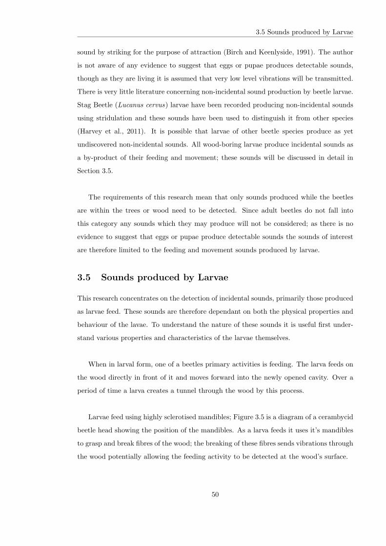
3.5 Sounds produced by Larvae
sound by striking for the purpose of attraction (Birch and Keenlyside, 1991). The author
is not aware of any evidence to suggest that eggs or pupae produces detectable sounds,
though as they are living it is assumed that very low level vibrations will be transmitted.
There is very little literature concerning non-incidental sound production by beetle larvae.
Stag Beetle (Lucanus cervus) larvae have been recorded producing non-incidental sounds
using stridulation and these sounds have been used to distinguish it from other species
(Harvey et al., 2011). It is possible that larvae of other beetle species produce as yet
undiscovered non-incidental sounds. All wood-boring larvae produce incidental sounds as
a by-product of their feeding and movement; these sounds will be discussed in detail in
Section 3.5.
The requirements of this research mean that only sounds produced while the beetles
are within the trees or wood need to be detected. Since adult beetles do not fall into
this category any sounds which they may produce will not be considered; as there is no
evidence to suggest that eggs or pupae produce detectable sounds the sounds of interest
are therefore limited to the feeding and movement sounds produced by larvae.
3.5 Sounds produced by Larvae
This research concentrates on the detection of incidental sounds, primarily those produced
as larvae feed. These sounds are therefore dependant on both the physical properties and
behaviour of the lavae. To understand the nature of these sounds it is useful first under-
stand various properties and characteristics of the larvae themselves.
When in larval form, one of a beetles primary activities is feeding. The larva feeds on
the wood directly in front of it and moves forward into the newly opened cavity. Over a
period of time a larva creates a tunnel through the wood by this process.
Larvae feed using highly sclerotised mandibles; Figure 3.5 is a diagram of a cerambycid
beetle head showing the position of the mandibles. As a larva feeds it uses it’s mandibles
to grasp and break fibres of the wood; the breaking of these fibres sends vibrations through
the wood potentially allowing the feeding activity to be detected at the wood’s surface.
50
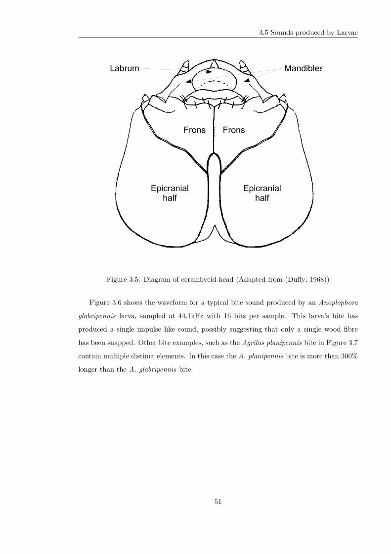
3.5 Sounds produced by Larvae
Figure 3.5: Diagram of cerambycid head (Adapted from (Duffy, 1968))
Figure 3.6 shows the waveform for a typical bite sound produced by an Anoplophora
glabripennis larva, sampled at 44.1kHz with 16 bits per sample. This larva’s bite has
produced a single impulse like sound, possibly suggesting that only a single wood fibre
has been snapped. Other bite examples, such as the Agrilus planipennis bite in Figure 3.7
contain multiple distinct elements. In this case the A. planipennis bite is more than 300%
longer than the A. glabripennis bite.
51

3.5 Sounds produced by Larvae
0 0.002 0.004 0.006 0.008 0.01 0.012 0.014 0.016−0.04
−0.03
−0.02
−0.01
0
0.01
0.02
0.03
0.04
Time (Seconds)
Am
plitu
de
Figure 3.6: An Anoplophora glabripennis bite
0 0.005 0.01 0.015 0.02 0.025 0.03 0.035 0.04 0.045−0.4
−0.3
−0.2
−0.1
0
0.1
0.2
0.3
0.4
Time (Seconds)
Am
plitu
de
Figure 3.7: An Agrilus planipennis bite
52

3.5 Sounds produced by Larvae
3.5.1 Variation within species
Relatively little is known about the variation in feeding behaviour of larvae or the sounds
associated with it. It is however likely that the feeding behaviour will be influenced by a
number of internal and external factors.
As a larva grows it progresses through a number of distinct stages. Insects in their
larval form replace their exoskeletons (Esperk et al., 2007), and the Latin word ’Instar’ is
used to define the period between these replacements (Fischer, 1853). As a larva progresses
into later instars it becomes physically larger. There are a number of ways in which this
growth could affect feeding and the incidental sounds associated with it. A later instar
larva will have larger mandibles and may be able to grasp a greater number of wood fibres
and exert a greater force on them than an earlier instar larva. It is also possible that the
feeding patterns will change as a larva develops, making it feed more or less frequently. In
the case of A. glabripennis, larvae feed on different parts of the host wood as they develop
through their Instars (Herard et al., 2009a).
Another consideration is the lifecycle of the insect. The life cycles of A. chinensis, A.
glabripennis and Agrilus planipennis are discussed in sections 3.6.2, 3.7.2 and 3.8.2. The
development and life-cycle of beetles is influenced by temperature. The effects of tempera-
ture variation on Anoplophora glabripennis were studied by Keena and Moore (Keena and
Moore, 2010). They found that larvae would only develop at temperatures below 30 C
and estimated that the minimum required temperature was 12 C. A similar study on
the effects of temperature variation on A. malasiaca was undertaken by Adachi (Adachi,
1994). Sets of larvae were kept at three temperatures: 20, 25 and 30 C. No larvae kept
at 25 or 30 C survived to the pupal stage.
Adachi also observed that ”most larvae spent a several-month period without feeding
before pupation”. This suggests a potential problem for a system based upon acoustic de-
tection, namely that larvae may spend significant periods of time producing no detectable
acoustic emmissions. Larvae detection in these situations would require an active detec-
tion method such as X-ray or ultrasound reflection. Fleming Et al studied the detection of
A. glabripennis larvae using non-contact 200kHz ultrasound imaging and concluded that
the technique was not currently feasible (Fleming et al., 2005). The limitations of X-ray
53

3.5 Sounds produced by Larvae
technology for larvae detection have been discussed in Chapter 2.
Numerous other factors could potentially influence the feeding behaviour and devel-
opment of larvae, such as wood moisture content or the species of the host. There are a
great deal of unknowns regarding the behaviour of larvae, largely due to their inaccessi-
bility when inside tree trunks.
3.5.2 Variation Between Species
In order for acoustic based species classification to be carried out the feeding sounds
produced by larvae of different species must be sufficiently different from one another
either in content or pattern of occurrence. In his 2007 thesis, Farr published classification
success rates of over 96% between two beetle species, Hylotrupes bajulus and Prionus
coriarius (Farr, 2007). These results suggest that there is a high degree of inter-species
variation in the feeding sounds produced. Species classification will be considered in detail
in Chapter 5.
54

3.6 Anoplophora chinensis (Citrus Long-Horned Beetle)
3.6 Anoplophora chinensis (Citrus Long-Horned Beetle)
A. chinensis is a wood boring beetle in the family Cerambycidae. A similar species,
Anoplophora malasiaca, is considered to be very closely related (EPPO, 2003), or in some
cases as a form of the same species (Lingafelter and Hoebeke, 2002).
Figure 3.8: Anoplophora chinensis adult (Image provided by FERA, used with permission)
3.6.1 Geographical Distribution
Both A. chinensis and A. malasiaca are native to East-Asia. A. chinensis is found in
China, Korea, Malaysia and Vietnam (EPPO, 2003). A. malasiaca is found in Japan
and Korea (Hu et al., 2009). Within the past decade several infestations and outbreaks
of A. chinesis have been found in Europe. These infestations are summarised in Table 3.2.
55

3.6 Anoplophora chinensis (Citrus Long-Horned Beetle)
Location Year Reference
Italy 2000, 2008 (Maspero et al., 2007), (Gaag et al., 2010)
France 2003 (Herard et al., 2006)
Croatia 2007 (Vukadin and Hrasovec, 2008)
Netherlands 2007, 2009 (Gaag et al., 2010)
Table 3.2: Anoplophora chinensis outbreaks in Europe
There have been no reported outbreaks in the United Kingdom however interceptions
have occured in 2005, 2008, 2009 and 2010 (FERA, 2011a).
3.6.2 Life Cycle
In it’s native East-Asia, A. chinensis has a lifecycle of approximately one year (Lieu,
1945). A. malasiaca has a lifecycle of between 1-2 years (Adachi, 1994). In the infestation
in Milan, Italy, a lifecycle of between 1 and 2 years has also been reported (Haack et al.,
2010).
Adults emerge between April and August but are most abundant between May and
July (FERA, 2008), (Maspero et al., 2007). Estimates vary from about 70 eggs laid per
female (EPPO, 2003) to over 300 (Adachi, 1988). Maspero et al. found that incubation
lasted between 15 and 20 days and is temperature dependant (Maspero et al., 2007). Exit
holes are usually found near the base of tree trunks or on roots (FERA, 2010).
3.6.3 Morphology
Stage Size Reference
Adult 25 - 35mm (EPPO, 2003)
Larva 50 - 60mm (Maspero et al., 2007)
Pupa 27 - 38mm (Lieu, 1945)
Egg 5 - 7mm x 1.7mm (Lieu, 1945), (Haack et al., 2010)
Table 3.3: Basic Dimensions of Anoplophora chinensis
56

3.7 Anoplophora glabripennis (Asian Long-Horned Beetle)
3.6.4 Hosts
A. chinensis has a large range of host plants (Gaag et al., 2010). These include Acer spp.,
Alnus spp., Betula spp., Casuarina spp., Citrus spp., Litchi spp., Malus spp., Populus
spp., Salix spp. and Ulmus spp. (EPPO, 2003), (FERA, 2008).
3.7 Anoplophora glabripennis (Asian Long-Horned Beetle)
The Asian long-horn beetle is native to China. Adults are around 3cm long, have black
with white spots and long black and white antennae. It’s larvae are white and worm-
like(USDA, 2007).
Figure 3.9: A. glabripennis adult (Image provided by FERA, used with permission)
3.7.1 Geographical Distribution
A. glabripennis is native to China and Korea (Hu et al., 2009). The first reported infesta-
tion outside Asia was in New York, USA, in 1996 (Haack et al., 1997). There have since
been several infestations reported across the US and in Europe (Hu et al., 2009). Table
3.4 gives a summary of these infestations.
57

3.7 Anoplophora glabripennis (Asian Long-Horned Beetle)
Location Year Reference
New York, US 1996 (Haack et al., 1997)
Chicago, US 1998 (Poland et al., 1998)
Braunau am Inn, Austria 2001 (Tomiczek et al., 2002)
New Jersey, US 2002 (Haack, 2003)
Toronto, Canada 2003 (Hu et al., 2009)
Gien, France 2003 (Herard et al., 2006)
Keukirchen am Inn, Germany 2004 (Benker et al., 2004)
Corbetta, Italy 2007 (Maspero et al., 2007)
Table 3.4: A. glabripennis outbreaks outside Asia
3.7.2 Life Cycle
Adults emerge between May and October (Li and Wu, 1993). Studies in China show that
the beetles can travel over 1400 metres from their exit holes with a mean dispersal distance
of 220-300 metres (Smith et al., 2000) to feed on leaves and young bark (EPPO, 2004).
Eggs are laid in individual oviposition pits below the bark (Li and Wu, 1993). Around 32
eggs are laid per female per season (Wong and Mong, 1986). Adults emerge leaving round
exit holes around 10mm in diameter. A. glabripennis uses both healthy and unhealthy
trees as hosts.
3.7.3 Morphology
Stage Size Reference
Adult 25 - 35mm (EPPO, 2004)
Larva up to 50mm (EPPO, 2004)
Egg 5 - 7mm (EPPO, 2004)
Table 3.5: Basic Morphology of A. glabripennis
3.7.4 Hosts
A. glabripennis has been found on a number of species of host trees in the US and China.
It primarily infests Populus spp., Salix spp., Ulmus spp. and Acer spp. (Haack et al.,
2006).
58

3.8 Agrilus planipennis (Emerald Ash-Borer)
Yang lists the major hosts of A. glabripennis in China as Populus nigra, Populus
deltoides, Populus dakhuanensis, Salix babylonica and Salix matsudana (Yang et al., 1995).
3.8 Agrilus planipennis (Emerald Ash-Borer)
The Emerald Ash-Borer is a member of the family Buprestidae. The adults are metallic
green coloured and infest Ash, usually causing death within 2 to 4 years of initial infesta-
tion. It is also known as Agrilus marcopoli and Agrilus feretrius. Adults leave distinctive
D shaped exit holes in the trees they infest as they emerge(Forestry-Commission, 2004).
Figure 3.10: Agrilus planipennis adult
Photograph: Pennsylvania Department of Conservation and Natural Resources -
Forestry Archive, Bugwood.org
3.8.1 Geographical Distribution
The species is native to parts of Asia; specifically northeastern China (Yu, 1992), Korea
(Ko, 1969) and Japan. It is also native to parts of far east Russia (Haack et al., 2002).
There are numerous infestations across the USA since 2002 including Illinois, Indiana, and
Ohio (APHIS, 2009). There have been no reported infestations in Europe. No intercep-
tions have been reported in the United Kingdom but the species is considered to be a
significant threat (Forestry-Commission, 2004).
59

3.9 Summary
3.8.2 Life Cycle
The entire life-cycle generally lasts 1 year although in some climates it can be 2 years
(Cappaert et al., 2005). There are 4 larval instars and adults emerge in May or early
June (Cappaert et al., 2005), (Wang et al., 2010). Approximately 10 days after emerging,
females begin to lay eggs (Wang et al., 2010). Between 60 and 90 eggs are laid per female
(Cappaert et al., 2005). Larvae feed under the bark in the cambium (See Figure 3.2)
(EPPO, 2005). Adults emerge from exit holes high up in the tree’s trunk or branches
(EPPO, 2005).
3.8.3 Morphology
Stage Length Width Reference
Adult 8.5 - 14.0mm 3.1 - 3.4mm (EPPO, 2005)
Larva 26 - 32mm 1.5 - 5.1 mm (EPPO, 2005),(Wang et al., 2010)
Pupa 11 - 16 mm 3-5 mm (Wang et al., 2010)
Egg 1 - 1.4 mm 0.8 - 1.1 mm (Wang et al., 2010)
Table 3.6: Basic Morphology of Agrilus planipennis
3.8.4 Hosts
As it’s name suggests, the Emerald Ash Borer primarily feeds on Ash (Fraxinus spp.).
Anulewicz et al. conducted a study to determine whether the beetle will feed on other
tree species and found that no beetles developed to adults on non-Ash species (Anulewicz
et al., 2008).
3.9 Summary
This chapter has discussed the source of the sounds which are to be detected. The trans-
mission of sound through would and properties which may effect this have been considered.
The categories of sounds produced by insects have been outlined along with the mech-
anisms which are used to produce them. The sounds produced by wood-boring beetle
species specifically have been considered and the feeding sounds produced by larvae inside
60

3.9 Summary
wood have been identified as the only suitable acoustical indicator of an infestation.
The chapter has concluded with case studies on three species of beetle, all of which
are considered to be INNS.
61

Chapter 4
Acoustic Monitoring and
Automated Detection
Automated acoustic detection can be considered as a two stage process; the first is the
monitoring or capturing of audio data by means of an acoustic sensor such as a micro-
phone or bi-morph. The second stage is the real-time analysis of the incoming audio data
to provide acoustic event extraction. This generalised model is represented in Figure 4.1.
This chapter begins by briefly describing the two categories of recording methods,
substrate and airborne, before examining the different methods which have been used to
monitor the acoustic emissions of wood boring pests. Section 4.1.2 covers the selection
of acoustic sensors and includes the results of testing which was used to compare their
performance.
Section 4.2 covers the task of automated detection and a number of methods by which it
can be performed. A novel technique known as Fractal Dimension Detection is introduced
in section 4.2.3 and its performance relative to other methods is investigated. The chapter
concludes with detection results.
4.1 Acoustic Monitoring
Bio-acoustics is a wide field ranging from the general, such as biodiversity assessment
(Sueur et al., 2008), (Riede, 1993), to the specific, such as the automated identification of
bird species (Chesmore, 2001) and crickets (Potamitis et al., 2007). Acoustics have been
62

4.1 Acoustic Monitoring
SensorRecordingDevice
EventExtraction
Hardware Software
Figure 4.1: Acoustic Monitoring and Detection Process
used as a method for monitoring various animals for several decades. The approaches
taken can be broadly separated into two groups, substrate and airborne. A substrate
recording is one in which the sensor is in contact (directly or indirectly) with the subject
being recorded. This method is most frequently used for monitoring insects but has
also been used for larger animals; examples include the bio-seismic monitoring of large
mammals (O’Connell-Rodwell et al., 2001) and acoustic monitoring of cattle (Clapham
et al., 2011). Airborne recording methods tend to be used when the subjects are likely
to move over a large area. The sensors used are often specialised to suit the type of
sound produced, such as the use of ultrasonic sensors to monitor bats (Vaughan et al.,
1997) and hydrophones to monitor sperm whales (Mellinger et al., 2002). This project
will concentrate on substrate recording methods since the subjects to be recorded are
contained within another substrate; the wood or timber, and have restricted movement.
4.1.1 Acoustic Monitoring of Insects in plants and timber
A number of acoustic monitoring methods have been used in the past to record the activity
of insect larvae in plants and timber. Brain suggested in 1924 that it may be possible to
detect insects in grain and fruit using acoustics (Brain, 1924).
Colebrook successfully recorded Xestobium rufovillosum larvae in timber using a piezo-
electric microphone (Colebrook, 1937). The sensors were placed on the surface of the
timber samples in a non-invasive manner.
Mankin et al. used an accelerometer to detect Cephus cinctus and Metamasius calli-
zona in Wheat and Bromeliads respectively (Mankin et al., 2004). One of the difficulties
63

4.1 Acoustic Monitoring
encountered with this method was attaining a suitably good interface between the ac-
celerometer and the sample plant. This can be attributed to the soft plant materials to
which the sensors were attached.
Fleming et al. used a non-contact ultrasonic sensor to detect Plectrodera scalator
larvae in wooden blocks. The technique was successful in detecting the drilled cavities in
the blocks but not the larvae placed inside them (Fleming et al., 2005).
A method sucessfully used by Mankin et al. to detect Anoplophora glabripennis in
trees used a combination of piezoelectric sensors attached to screws which were inserted
into the wood (Mankin et al., 2008). A disadvantage of this method is that it is invasive
and may not be feasible for use on high value trees.
Rohitha et al. used electret microphones to detect Oemona hirta larvae in wood (Ro-
hitha et al., 1994). This approach required the sample to be placed in an acoustically
isolated chamber in order to detect sounds produced by the larvae above background
noise. The isolation requirements and the use of a gain of 50000 mean that this method
could only be used in laboratory conditions.
Piezoeletric sensors were also used by Potamitis et al. to detect Rhynchophorus fer-
rungineus (Red Palm Weevil) (Potamitis et al., 2008). In this case the sensor probes were
inserted into the tree rather than being mounted on the surface.
Farr investigated a number of acoustic sensors for use in detecting beetle larvae (Farr,
2007) in hard and soft plant material. Sensors considered were bi-morphs, piezoelectric
transducers and microphones. He found that the bi-morph sensors were very fragile and
prone to breaking when being attached or removed from samples. Piezoelectric sensors
were concluded to be the most sensitive of the three investigated. Table 4.1 summarises
the sensors which have been used to record various insects in plants and timber. The term
invasive is used here to distinguish between those approaches which penetrate the surface
of the wood or plant material, and those that do not.
64

4.1 Acoustic Monitoring
Sensor Type Invasive Details Reference
Piezo-electric micro-
phone
No Detection of Xestobium
rufovillosum
(Colebrook, 1937)
Ultrasonic sensors No Monitoring of termites
in wood
(Fujii et al., 1990)
Electret microphone No Recording of Oemona
hirta in wood
(Rohitha et al.,
1994)
Accelerometer No Detection of Cephus
cinctus and Metamasius
callizona in Wheat and
Bromeliads
(Mankin et al., 2004)
Piezo sensors, bi-
morphs, microphones
No Detection of various
wood boring-beetle
species
(Farr, 2007)
Piezo sensors Yes Detection of
Anoplophora glabripen-
nis
(Mankin et al., 2008)
Piezo sensors Yes Detection of Rhyn-
chophorus ferrungineus
(Potamitis et al.,
2008)
Table 4.1: Summary of sensors used to detect insects in plants and timber
4.1.2 Sensor Selection and Coupling
The requirements for the sensors are that they are to be low cost, simple to attach and
provide a good acoustic coupling with the wood or tree. The attachment of the sensors
must be non-invasive, that is to say that they must not penetrate the surface or in any way
damage the sample. This restricts the range of attachment methods which can be used.
The use of waveguides inserted into the sample in order to improve acoustic coupling such
as those used by Mankin et al. is therefore not a viable option (Mankin et al., 2000).
An investigation into the efficiency of multiple types of sensors has been carried out.
Since the completion of the previous DEFRA project (PH0191) (Farr, 2007), multi-axis
accelerometers have decreased significantly in cost, to around £10 per unit. These sen-
sors could potentially be more sensitive than piezo-electric devices so a number of tests
65

4.1 Acoustic Monitoring
were carried out using them. Three sensor types were investigated using two experiments.
Figure 4.2 shows the equipment set-ups used. An Oak log had a hole drilled into one end
into which a speaker or solenoid was inserted. The sensor being tested was then attached
to the surface of the log, positioned directly above the cavity or at a defined distance
from it along the surface. The piezo sensors were attached to the log using elastic bands.
Attempts to attach the accelerometer circuit using this method resulted in no signal being
detected. The results below were obtained by holding the accelerometer circuit firmly
against the bark.
Log
Sensor
Speaker
(a) Embedded piezo-speaker
Log
Sensor
Solenoid
(b) Embedded solenoid
Figure 4.2: Sensor coupling experiment set-up
Table 4.2 lists the types of sensors tested. The first two sensors are simple piezo-
electric devices which are passive. The final sensor is a 2-axis accelerometer although only
a single axis was used. The accelerometer is a powered sensor which required mounting
on a printed circuit board.
Sensor Type Name Used Details Unit Cost
(Approx)
Murata PKLCS1212E2000-R1 Piezo Sensor 1 Square piezo with 2kHz
resonant frequency
£2
Kingstate KPEG116 Piezo Sensor 2 Circular piezo with 2kHz
resonant frequency
£1
Analog Devices ADXL322JCP Accelerometer 2-Axis Accelerometer £10
Table 4.2: Table of sensors tested
The first experiment used a piezo-speaker inserted into the log. Sine waves with am-
plitude 12V p-p, at various frequencies were played through the speaker and the voltage
66

4.1 Acoustic Monitoring
at the sensor recorded to assess the relative performance. The results are shown in Figure
4.3.
Figure 4.3: Voltage at sensor vs input frequency
The second experiment used a solenoid inserted into the log to provide a sound impulse
with a consistent amplitude. The sensors were placed at various distances from the solenoid
along the surface of the log. The results can be seen in Figure 4.4.
67
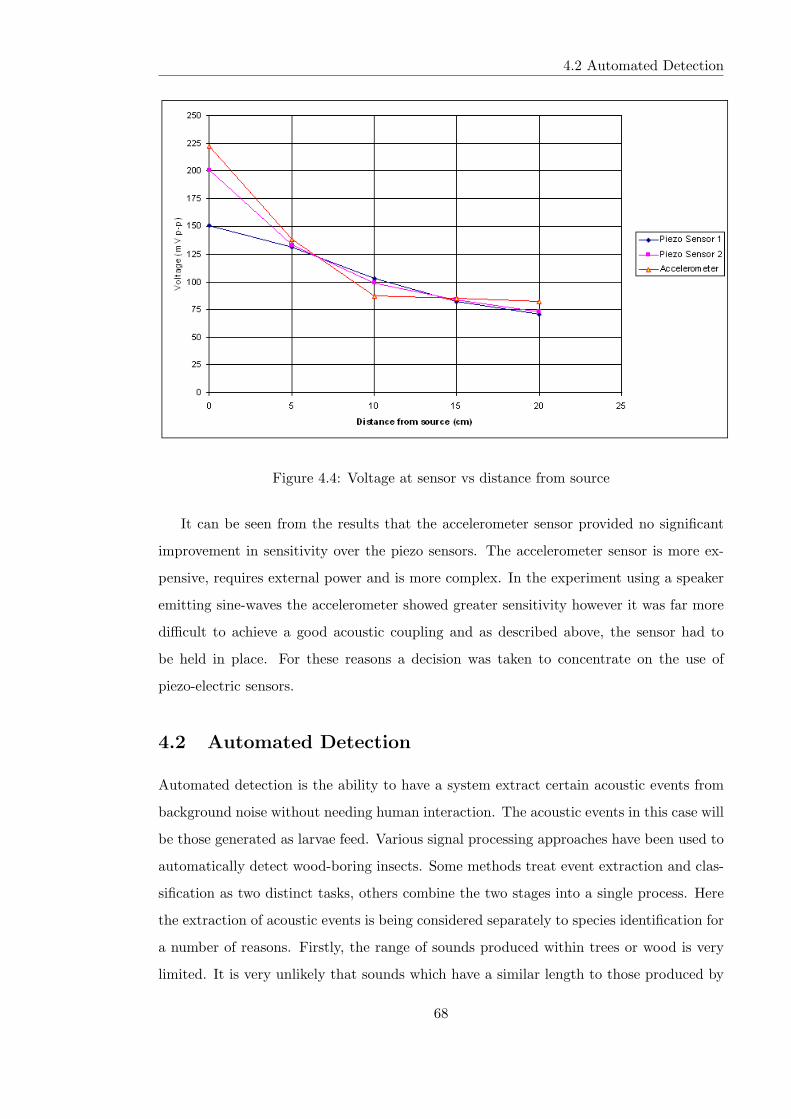
4.2 Automated Detection
Figure 4.4: Voltage at sensor vs distance from source
It can be seen from the results that the accelerometer sensor provided no significant
improvement in sensitivity over the piezo sensors. The accelerometer sensor is more ex-
pensive, requires external power and is more complex. In the experiment using a speaker
emitting sine-waves the accelerometer showed greater sensitivity however it was far more
difficult to achieve a good acoustic coupling and as described above, the sensor had to
be held in place. For these reasons a decision was taken to concentrate on the use of
piezo-electric sensors.
4.2 Automated Detection
Automated detection is the ability to have a system extract certain acoustic events from
background noise without needing human interaction. The acoustic events in this case will
be those generated as larvae feed. Various signal processing approaches have been used to
automatically detect wood-boring insects. Some methods treat event extraction and clas-
sification as two distinct tasks, others combine the two stages into a single process. Here
the extraction of acoustic events is being considered separately to species identification for
a number of reasons. Firstly, the range of sounds produced within trees or wood is very
limited. It is very unlikely that sounds which have a similar length to those produced by
68

4.2 Automated Detection
larvae will be produced within a tree or cut wood. The primary aim of the system is to
detect larvae rather than to identify their species. It is important that the system can de-
tect bites with amplitudes as low as possible which may not contain sufficient information
above the noise level to enable successful species identification. The proportion of audio
information which is related to larval feeding as opposed to noise is very low; since the
system is to be implemented in real-time, this seperation of tasks will be needed to limit
the amount of data which is passed on to the species identifier.
A computationally simple system was used by Webb et al. to detect larvae recorded
in fruit and grain (Webb et al., 1988). Samples were placed in a sound insulated chamber
and the recordings made passed through a band-pass filter. A simple amplitude threshold
was then sufficient to detect larval activity within the recording.
Mankin et al. used a combination of amplitude thresholds, spectral profiling and
temporal pattern analysis for the automated detection and identification of Anoplophora
glabripennis (Mankin et al., 2008). Recorded audio was first band-pass filtered between
200Hz and 5kHz. An amplitude threshold was defined as a multiple of a moving average of
the amplitude using 0.186s intervals. When this threshold was exceeded a power spectrum
was generated using a 512 sample Fast Fourier Transform centred about the largest peak
within the next 6ms of audio. This power spectrum data was then either used to create
a spectral profile or to classify against a spectral profile already in existence. Spectral
profiles were generated by comparing the current power spectrum against that in the pro-
file. If the mean of the squared differences between spectrum levels was below a predefined
threshold the current power spectrum would be in the profile. Classification used a similar
predefined threshold to determine whether the power spectrum of a detected impulse was
closed enough to the profile.
4.2.1 Energy Detection
Ultra short time energy detection (USTED) was used by Potamitis to extract acoustic
events from recordings of crickets (Potamitis et al., 2006). Recognition rates of non-
incidental stridulation sounds of around 95% were obtained using this method. Farr
adapted USTED for the extraction of incidental sounds produced by larvae bites (Farr,
69

4.2 Automated Detection
2007). This required the frame size to be increased in order to successfully detect the
lower amplitude larval bites.
The method itself relies on the assumption that an acoustic event has an energy content
which is sufficiently higher than the average for the recording. The energy of successive
segments of audio is measured and a threshold is applied to determine whether a segment
contains or forms part of an acoustic event. Audio data is separated into M frames of a
fixed length:
M = N/L (4.1)
where N is the total number of samples and L is the frame length in samples. The energy
for each frame, Euse(k) is then estimated using:
Euse(k) =L∑
i=1
[x(kL+ i)]2, k = 0, ...,M − 1 (4.2)
where Euse(k) is the estimated energy for frame k, L is group size, M is the number of
frames and x is the audio data (Potamitis et al., 2006).
The group sized used should be selected based upon the length of event which is being
detected. Potamitis used a group size of 5 samples, 113µs at 44.1kHz (Potamitis et al.,
2006). In order to use this method to detect low level incidental sounds produced by
beetle larvae, Farr increased the group size to 44 samples, around 1ms at 44.1kHz (Farr,
2007). Figure 4.2.1 shows an example bite with energy values calculated using this method
overlayed.
70

4.2 Automated Detection
0 0.02 0.04 0.06 0.08 0.1
−0.1
0
0.1
0.2
Time (Seconds)
Am
plitu
de
0 0.02 0.04 0.06 0.08 0.10
1
2
3
4
5
6
Ene
rgy
Figure 4.5: Bite with energy overlayed
4.2.2 Fractal Dimension
Fractal dimension has been used as a tool for analysis of various acoustic signals. Most
commonly it is used to analyse waveforms over a relatively long period of time such as
those produced by monitoring organ activity and function. Yambe et al. used fractal
dimension to detect variations in cardiac function. This approach was used due to the
non-linearity of heart rate variability (Yambe et al., 1999). Similar techniques were later
used to analyse changes of fetal heart rate during pregnancy and by (Hotta et al., 2005)
to analyse heart rate variability and mortality in the elderly. A fractal dimension based
approach using Higuchi’s algorithm has also been used to compare the electrocortical ac-
tivity of rat brains before and after injury (Spasic et al., 2005).
Each of these applications uses fractal dimension to analyse changes of complexity in
non-linear waveforms. Fractal dimension has the potential to be used for acoustic event
detection if the event in question has a suitably differing complexity to the surrounding
noise. Extracting acoustic events using fractal dimension detection relies on the concept
that shapes can have a non-integer, or fractal, dimension. The fundamental concepts be-
hind fractal dimension will be explained in here and their application to event detection
71

4.2 Automated Detection
in the next section.
By the late 19th century, mathematicians had determined that the definition of dimen-
sion as an integer number of coordinates was unsatisfactory (Cantor, 1890). To understand
non-integer dimension it is necessary to determine a mathematical basis from which our
concept of the traditional ’1 , 2 and 3’ dimensions is derived. This is most simply ap-
proached by considering self-similarity. A line, for example, is one dimensional and can be
doubled in length to produce two self similar shapes. A square can be doubled in length
and width to produce four self similar shapes. Similarly a cube can be doubled in height,
length and width to produce eight self similar shapes (Lanius, 2007). Table 4.2.2 shows
these shapes, their dimensions and the number of self similar copies generated when scaled
by a factor of two.
Shape Dimension Self Similar Copies Scaling Factor
Line 1 2 2
Square 2 4 2
Cube 3 8 2
Table 4.3: The dimensions of common geometric shapes
This non-integer understanding of dimension was formalised by Hausdorff in 1919 and
is known as the Hausdorff Dimension (Hausdorff, 1919). The dimension can be defined as:
D =log(N)
log(r)(4.3)
where N is the number of self similar shapes and r is the scaling factor (Devaney, 1995).
This concept was later developed and the term fractal dimension coined to describe
the non-integer dimension of geometric shapes (Mandelbrot, 1983). It can be applied to
complex geometric shapes to calculate a non-integer dimension. The Sierpinski triangle
(Figure 4.6), for example, appears to the eye to have a dimension of somewhere between
one and two.
72

4.2 Automated Detection
Figure 4.6: Sierpinski Triangle
Equation 4.3 can be applied to Sierpinski’s Triangle using either of the scaling factors
and self similar shape numbers given. The dimension can then be calculated as:
log(9)
log(4)=
log(3)
log(2)= 1.59 (4.4)
Fractal dimension can also be easily calculated for self-similar curves. The Koch curve
(Figure 4.7) (Koch, 1904) is a self similar curve which can be generated from a straight
line by the iterative process described below:
73

4.2 Automated Detection
1. Divide the line into three equal lengthed segments.
2. Form an equilateral triangle pointing upwards using the middle segment as a base.
3. Remove the original middle segment.
Figure 4.7: Koch Curve
The fractal dimension for the Koch curve can be calculated using equation 4.3 as:
log(4)
log(3)= 1.26 (4.5)
74

4.2 Automated Detection
The fractal dimension value of a shape can be considered to provide an estimate of it’s
complexity (Hitchcock, 2003).
4.2.2.1 Methods for estimating the fractal dimension of time-series
Fractal dimension is difficult to calculate directly and several different methods of esti-
mation are used (Schepers et al., 1992), (Esteller et al., 2001). One of the most widely
used fractal dimension estimation methods was published by Higuchi in his 1988 paper
(Higuchi, 1988). For a time series with N values, X(1), X(2), ..., X(N), k new time series
are constructed where m = 1, ..., k:
Xmk = X(m), X(m+ k), X(m+ 2k), ..., X(m+
[
N −m
k
]
· k) (4.6)
The length of the curves, Lm(k), are then calculated using equation 4.7.
Lm(k) =1
k
[N−m
k]
∑
i=1
|X(m+ ik)−X(m+ (i− 1) · k)|
N − 1[
N−mk
]
· k
(4.7)
L(k), the length of the curve for the time interval k, is calculated as the average of all
Lm(k) curves:
L(k) =1
k·
k∑
m=1
L(m, k) (4.8)
D, the estimated fractal dimension, is the slope of a log/log plot of L(k) against 1/k cal-
culated by least-squares fit.
Another commonly used method was proposed by Katz (Katz, 1988). For a curve
containing N values, x0 ... xN , the length, L, is calculated as the sum of the distances
between adjacent points.
L =
N−1∑
i=1
dist(i, i+ 1) (4.9)
D, the estimated fractal dimension, is calculated using equation 4.10 where d is the max-
imum distance between any two points on the curve.
75

4.2 Automated Detection
D =log(N − 1)
log(N − 1) + log( dL)
(4.10)
In his 1998 paper Sevcik proved that Katz’ method was flawed in that as N , the number
of samples, is increased, the estimated fractal dimension tends to 1 (Sevcik, 1998). Sevcik
produced an alternate method to overcome this. For a given waveform containing N
values, x0, ..., xN , an approximation to the fractal dimension is calculated using the
following method. The waveform is first normalised in both axes and mapped to a unit
square using equations 4.11 and 4.12.
x∗i =xi
xmax(4.11)
y∗i =yi − ymin
ymax − ymin(4.12)
L, the length of the curve in the unit square is calculated by summing the distances
between adjacent normalised points (Equation 4.13).
L =N−1∑
i=1
dist(i∗, (i+ 1)∗) (4.13)
D, the approximate fractal dimension of a waveform, is calculated using equation 4.14.
D = 1 +ln(L)
ln(2 ∗ (N − 1))(4.14)
In order for an estimation method to be useful for event detection it does not necessarily
need to produce a highly accurate estimate of fractal dimension. Since the end system
needs to perform the event detection task in real-time, an algorithm was selected based
upon computational simplicity rather than mathematical accuracy. Using big-O notation,
Higuchi’s algorithm has a complexity of O(N2) whereas Sevcik’s has a complexity of O(N).
In practice ’real-time’ means that detection results are provided to the user at one
second intervals since the average fractal values, as used in equation 4.15 are calculated
76

4.2 Automated Detection
using one second long chunks of audio. The system as a whole must therefore be able to
analyse each chunk of audio before another is presented. On modern PC hardware the
time taken for fractal dimension analysis calculation is insignificant since it is in the order
of milliseconds. It is however, envisaged that the detection methods may be implemented
on embedded hardware with significantly lower processing power in the future. For these
reasons, Sevcik’s method was chosen for use in the detection system.
4.2.3 Fractal Dimension Detection
Acoustic events can be detected using fractal dimension by segmenting the waveform in
a similar way to USTED. Audio is segmented into frames of equal length and the fractal
dimension of each frame calculated using equations 4.11 to 4.14. A threshold is then
applied to these values to determine whether a frame contains an acoustic event. Figure
4.2.3 shows an example bite with fractal dimension values overlayed.
0 0.02 0.04 0.06 0.08 0.1
−0.1
0
0.1
0.2
Time (Seconds)
Am
plitu
de
0 0.02 0.04 0.06 0.08 0.11.3
1.4
1.5
1.6
Fra
ctal
Dim
ensi
on
Figure 4.8: Anoplophora glabripennis bite with Fractal Dimension overlayed (Frame size
200 samples)
4.2.4 Comparison of detection methods
In order to compare the two bite detection methods a number of sample audio files were
generated to test the relative performance of each method.
77

4.2 Automated Detection
One hundred individual bite sounds were extracted from recordings and each was
placed at a known position into one second long audio clips consisting entirely of white
noise. Each bite was merged with noise at multiple different signal to noise ratios to gen-
erate a set of five hundred sample audio files with which to test the detection methods.
A second test using automatically generated 1kHz sine waves of length 10 milliseconds,
in place of real bite sounds was also performed to the same test specifications. The fre-
quency and length of the sine wave were chosen to give it similar properties to a real larval
bite albeit without any decay over time. It also enabled a direct comparision between the
performance of the two methods using a strictly defined repeatable input.
Fractal dimension and energy values were calculated for each frame within the test
waveform. The fractal dimension and energy values for the first frame containing the
’event’ were measured as distance from the mean value in multiples of the standard devi-
ation according to equations 4.15 and 4.16.
Fdist =|Devent −D|
σ(4.15)
Edist =|Eevent − E|
σ(4.16)
Figures 4.9 and 4.10 show Edist and Fdist plotted against signal to noise ratio for
embedded bites and embedded sine wave respectively.
78

4.2 Automated Detection
2 4 6 8 10 12 14 16 18 202
4
6
8
10
12
14
16
Signal to Noise Ratio (dB)
Mul
tiple
s of
SD
from
mea
n va
lue
Fdist
Edist
Figure 4.9: Fractal Distance and Energy Distance vs Signal to Noise Ratio (Embedded
Bites, Frame Size 200 Samples)
0 2 4 6 8 10 12 14 16 18 205
6
7
8
9
10
11
12
Signal to Noise Ratio (dB)
Mul
tiple
s of
SD
from
mea
n va
lue
Fdist
Edist
Figure 4.10: Fractal Distance and Energy Distance vs Signal to Noise Ratio (Embedded
Sine Wave, Frame Size 200 Samples)
Ultra short time energy outperforms fractal dimension in terms of distance from mean
value when detecting high signal to noise ratio events. This does not however suggest
that energy detection provides any advantage in terms of detection since both Fdist and
Edist at high signal to noise ratio are clearly sufficient for detection. At lower signal to
noise ratios fractal dimension outperforms energy detection for both embedded bites and
79

4.2 Automated Detection
embedded the sine wave. This is significant since at these low signal to noise ratios Fdist
and Edist are closer to the threshold level so the advantage that fractal dimension has in
terms of distance from mean value will enable bite detection at lower signal to noise ratios.
At a signal to noise ratio of 4, the embedded bites produces fractal values which are
on average 9.77 standard deviations away from the mean whereas the equivalent mean
energy detection value is only 4.22. At a signal to noise ration of 2, the figures are 6.61
for fractal dimension and 2.03 for energy detection; representing a 3.26 factor advantage.
4.2.5 Frame sizing
The frame size used to segment the waveforms will have an impact on the ability to dis-
tinguish between bites and background noise. To measure this effect the audio files with
10dB signal to noise ratio events from the previous test were analysed using varied frame
sizes. Figures 4.11 and 4.12 show the results of this analysis. In both cases the x-axis
is the frame size multiple which is calculated using the average event length over all test
audio files.
10−1
100
101
0
1
2
3
4
5
6
7
8
9
10
Frame Size Multiple
Ddi
st
Figure 4.11: Fractal Distance vs Frame Size Multiple for embedded sine wave at 10dB
80

4.2 Automated Detection
10−1
100
101
2
4
6
8
10
12
14
Frame Size Multiple
Ddi
st
Figure 4.12: Fractal Distance vs Frame Size Multiple for embedded bites at 10dB
In both cases Ddist decreases significantly when the frame size multiple is greater than
one. In these situations each frame contains a proportion of audio containing purely noise
which causes Devent to be closer to D. The value of Ddist for the embedded sine wave
remains relatively stable for frame size multiples less than one. Given the cyclic nature of
the wave this is unsurprising since the fractal dimension should be constant throughout it’s
length. If the frame size were to be decreased further it could be expected that Ddist will
decrease as the low number of samples negatively affect the accuracy of fractal dimension
estimation.
The peak Ddist value for the embedded bites is found when the frame size multiple is
0.6 and then decreases with frame size. The fractal dimension of a bite varies throughout
it’s length and the most useful portion in terms of event detection appears to be in the
centre. This result demonstrates that the most effective way of detecting bite events may
be to use a smaller frame size than the average bite length and to expand the event by a
fixed number of samples either side.
4.2.6 Vertical Threshold
The level at which the Ddist threshold is set is crucial in achieving optimum bite detection
performance. If set too high, bites will be left undetected, if set too low segments of noise
81

4.2 Automated Detection
may be falsely detected as bites.
Bite detection is performed by segmenting the incoming audio into blocks one second
in length. Each block is then further segmented into frames and the FD calculated for
each frame. The distance from mean for each frame is then calculated using Equation 4.17
where D is the fractal dimension for the current frame and D is the mean over all frames
within the block.
Ddist =|D − F |
σ(4.17)
In order to determine the optimum Ddist threshold level the performance of the de-
tection system over a range of threshold levels has been tested. The rate of false posi-
tive detection was measured using artificially generated white noise and ambient sound
recorded in a vacant laboratory. The rate of true positive detection of bites was measured
using a recording of A. glabripennis. The relationship between detection rates and vertical
threshold is shown in Figure 4.13.
Figure 4.13: Detection of random noise, ambient noise and bites
It can be seen from the graph that in order to achieve no false detections in random
and ambient noise a threshold of above 4 is required. The true negative detection in
82

4.2 Automated Detection
ambient noise rate at a threshold of 3 is 99.56%; this figure suggests that the distribution
of FD values has a normal distribution when the audio itself is normally distributed. At
a threshold level of 3, all bites were sucessfully detected, however a small percentage of
noise is falsely detected as bites. The ideal threshold level depends upon the needs of the
user in terms of the relative importance of false negatives and false positives. The system
being developed here is intended to be used alongside other larvae detection techniques
which are currently used by DEFRA. Since part of the motivation for this work is the risk
of false negative results from current techniques, a threshold of 3 was selected to minimise
false negative results from this system.
4.2.7 Horizontal Threshold
Horizontal thresholding is applied in order to reduce the number of false positive results.
A maximum event length, EMAX is defined to prevent the detection of events which are
too long to be attributed to the feeding of larvae. The value of EMAX is dependant on
the frame length selected and is a multiple of frame length.
4.2.8 Bite Padding
Since the detection method does not use any overlapping of frames it is necessary to expand
the detect events at both ends to ensure that the acoustic activity is fully captured. Figure
4.14 shows the best and worst cases of frame positioning relative to the bite where the
frame size is half of the bite duration. The original output from the vertical thresholding
of frames is shown by the thick black line; each event is then expanded by the length of
one frame at either end as shown by the thick red line. In the best case this results in the
unnecessary expansion of the event to include noise; however this additional data should
have no detrimental effect since it will be ignored by the species recognition method.
83

4.2 Automated Detection
Figure 4.14: Event Expansion
4.2.9 Example Activity
Figure 4.15 shows the detection results for a recording of an unidentified larva over a
long time period. This example shows how larval activity can vary over time; the period
between 21:00 and 22:00 contains significantly less activity, for unknown reasons. The
recording also appears to show that activity gradually increases at the start of the record-
ing, this behaviour occurs in other recordings which have been made during this research
and may indicate that larvae are sensitive to the movement and noise produced when
attaching sensors.
Figure 4.15: Activity of unknown larva over 20 hour period
84

4.3 Dual Sensor
4.3 Dual Sensor
False positive events cannot be eliminated entirely by means of horizontal and vertical
thresholding. In recordings in a laboratory environment, false positives may be introduced
by electrical switching noise for example. In field recordings sounds produced by exter-
nal activity such as twigs breaking may be of short enough duration to trigger false events.
In order to further limit the number of false positive results produced a simple dual
sensor technique was devised. Its implementation adds little additional computational or
monetary cost to the system. Physically the secondary sensor is identical to the primary
sensor and is connected to the spare channel on the USB audio device. This second sensor
is used to detect ambient sound and is not attached to the sample material.
Fractal Dimension analysis is performed on the second channel in exactly the same way
as on the primary channel. For each segment of audio data, two events lists are therefore
produced. The events on the secondary channel are used to cancel any events which occur
in the same position on the primary channel since it is likely that such events are not the
result of larval feeding activity. The implementation of the dual sensor system is covered
in greater detail in Chapter 6.
4.4 Summary
This chapter has covered the methods used to acoustically detect larvae. Recording and
monitoring methods which have been used by others have been considered and two types
of acoustic sensor have been investigated.
The computational methods which have been used for acoustic event detection have
been reviewed and a new technique based upon Fractal Dimension (FD) analysis is intro-
duced. The background to FD and methods which are used in its estimation have been
described and the performance of FD detection and short time energy detection has been
compared. FD detection has been shown to enable the detection of events at lower signal
to noise ratios. Finally the vertical and horizontal thresholding process and the use of a
secondary sensor for the reduction of false positive events has been described and results
provided for varied detection threshold levels.
85

4.4 Summary
86

Chapter 5
Species Identification
The task of automated identification or pattern recognition has been applied to a wide
range of problems using numerous diverse methods (Ripley, 1996), (Theodoridis and Kout-
roumbas, 2003). The terms are used to describe a process by which sets of input data are
grouped based upon their similarities into user-defined or machine-created classes which
can be used to represent some form of meaningful output category.
Despite the wide range of methods used, the task can usually be generalised as a pro-
cessing having two distinct stages - feature extraction and classification. In it’s simplist
form, feature extraction is the selection of the most useful information from the input
data. Classification is the process by which this information is placed into the most ap-
propriate output category. Perhaps confusingly, the term classifcation is also often used
to encompass the entire pattern recognition task (Brown and Miller, 2007), (Lee et al.,
2003), (Waser et al., 2011).
This chapter covers these two stages of pattern recognition separately and investigates
the approaches taken by others for the purpose of automated acoustic identification of
beetles and other insects.
5.1 Feature extraction
Feature extraction is the first stage in the automated classification process. It is the means
by which the most useful elements or features are selected from the input data for classi-
fication. An ideal feature extraction method will select those features which exhibit the
87

5.1 Feature extraction
greatest variation between classes whilst maintaining the closest similarity within classes.
The dimensionality of the input data will be reduced as features are extracted, by dis-
carding input data, and generated, by combining data. This dimensionality reduction is
important since a classifier will suffer if provided with excessively large dimension data as
well as data with inadequate dimension. The process decreases the number of parameters
which are used in the classifier, allowing better generalisation (Bishop, 1995). That is to
say the classifier will have a greater ability to cope with variations of data which are within
classes. There are also obvious computational benefits to dimensionality reduction, namely
fewer calculations and a lower memory requirement for input data and classifier storage.
The selection of a computationally efficient feature extraction technique is of particular
importance to this project since it is necessary that classification is performed in real-time.
The remainder of this chapter will look at the various techniques which have been
employed by others for use in the automated acoustic identification of beetles, animals
and sound in general. In particular, the techniques used in DEFRA project PH0191
will be investigated. Table 5.1 lists feature extraction methods which have been used to
analyse sounds produced by beetle larvae; the letters D and I in the task column represent
Detection and Identification.
Species Feature Extraction
Method
Task Reference
Rhynchophorus ferrugineus Filterbank D (Pinhas et al., 2008)
Rhynchophorus ferrugineus Short-time Fourier
Transform & Dis-
crete wavelet packet
transform
D (Potamitis et al.,
2008)
Rhynchophorus ferrugineus Time Frequency Dis-
tribution
D (Al-Manie and
Alkanhal, 2005)
Various species Time Domain Signal
Coding
I (Farr, 2007)
Anoplophora glabripennis Spectral Profile and
Temporal Patterns
D (Mankin et al., 2008)
Table 5.1: Feature extraction methods used in the analysis of beetle larvae sounds
88

5.1 Feature extraction
5.1.1 Spectral Profiling
Mankin et al. used a frequency domain technique for the detection of Asian Longhorn
Beetle larvae (Mankin et al., 2008). The feature extraction stage of the technique was spec-
tral estimation by means of the Discrete Fourier Transform (DFT). The DFT is widely
used for spectral analysis and is used to generate a power spectrum from a discrete signal,
providing information on the relative power of different frequency components within the
signal.
The DFT assumes that signals are circular, therefore care must be taken when se-
lecting an appropriate windowing function to prevent the introduction of false frequency
information. The Fast Fourier Transform (FFT) algorithm is commonly used because of
its relative computational efficiency (Cooley and Tukey, 1965). It requires that the signal
length is a power of two; shorter signals can be increased to the required length by zero
padding.
5.1.2 Filterbank Analysis
Pinhas et al. used filterbank analysis for the feature extraction stage of an acoustic de-
tection system for Red Palm Weevil (Rhynchophorus ferrugineus), acheiving up to 98.8%
detection rates (Pinhas et al., 2008). Their technique involves first dividing the input sig-
nal into fixed lengthed frames with 50% overlap. After applying an amplitude threshold
to discard frames which were considered to be noise, the DFT of each frame is calculated
and a Hamming window applied.
Filterbanks are used to reduce the dimensionality of spectral data by smoothing and
frequency selectivity. A set of band pass filters, which may vary in position and scale, are
multiplied with the spectral data to produce an average energy value for each band (Bimbot
et al., 2004). A commonly used filter bank technique is the Mel-frequency cepstrum (MFC)
which leads to the generation of Mel-frequency cepstral coefficients (MFCCs). The spacing
of filters is based upon the MEL scale, which was devised by Stevens and Volkman and is
based upon the human perception of sound (Stevens et al., 1937). MFCCs are frequently
used for the analysis of human speech and speaker recognition (Bimbot et al., 2004),
(Kamruzzanman et al., 2007), (Viikki and Laurila, 1998).
89
5.1 Feature extraction
5.1.3 Short Time Fourier Transform (STFT)
Al-Manie and Alkanhal used this time-frequency domain feature extraction technique for
the detection of Red Palm Weevil (Al-Manie and Alkanhal, 2005). The paper does not list
any detection results; however the method employed is commonly used in audio analysis
and therefore is included here.
The STFT is used to produce a time-frequency distribution by first segmenting the
signal into frames of fixed length using a windowing function to minimise the introduction
of errors, then applying the DFT (Section 5.1.1) to each frame (Hlawatsch and Auger,
2008). The fixed resolution of the STFT is a limitation as there is a trade-off between
frequency resolution and time resolution. Narrow frames allow for better time resolution
at the expense of frequency resolution; wide windows provide better frequency resolution
at the expense of time resolution. Additionally, for any signal there is a minimum window
width for which meaningful frequency information can be generated (Cohen, 1995).
5.1.4 Fractal Dimension
The possibility of using fractal dimension (FD) values as a feature for bite species clas-
sification is considered here because these values are already calculated during the bite
detection process described in Chapter 4. A species identification method which could
use these values would be advantageous since the extra computing time required would
be minimal.
To assess the suitability of discriminating between bites produced by different species
by this method the FD values for a number bites from various beetle species were cal-
culated. A histogram of these values can be seen in Figure 5.1. These results show a
significant overlap between the ranges of FD values of bites; based upon this data it was
concluded that fractal dimension values alone are not suitable for use in the separation of
bite sounds produced by different beetle species.
5.1.5 Time Domain Signal Coding (TDSC)
Farr (2007) used a technique known as Time Domain Signal Coding (TDSC) for the fea-
ture extraction stage of an acoustic larvae identification system (Farr, 2007). This work
differs from most of the other methods covered here in that it is used to perform iden-
90

5.1 Feature extraction
Figure 5.1: Distribution of FD Values
tification of species (classification between different species) rather than simply detection
(classification between insect and noise).
The technique originates from a time domain method for the compression of speech
data, Time Encoded Speech (TES) (King and Gosling, 1978). This was then developed
into Time Encoded Signal Processing (TESPAR) by King some years later (King, 1995).
TESPAR was first used in the analysis of insect sounds by Chesmore et al. (Chesmore
et al., 1997).
Time Domain Signal Coding (TDSC) aims to represent the characteristics of a given
waveform by its shape and duration values between successive zero crossings; termed an
epoch. Shape values are calculated as the number of positive minima or negative maxima
while duration is simply the number of samples between the given zero crossings. Figure
5.2 shows an example waveform with annotated TDSC calculations. The waveform can
be seen to have two epochs, each encoded with shape and duration information. The first
epoch is positive and contains a single minimum giving it a shape value of 1. The second
is negative and contains two maxima, giving it a shape value of 2.
91

5.1 Feature extraction
Figure 5.2: Example of waveform epochs (D1,S1) and (D2,S2)
Adapted from (Chesmore, 2001).
Shape and duration values are then combined to produce a single code value for each
epoch within the waveform, either by using a code-book or equation. An example code-
book is shown in Figure 5.3.
Fixed codebooks can be a limitation in TDSC since they may result in the failed en-
coding of certain complex waveform features, such as unusually high numbers of minima
in an epoch, due to the lack of codes to represent them (Farr, 2007). Swarbrick attempted
to overcome this limitation by introducing a technique which would select appropriate
codebooks automatically (Swarbrick, 2001). Farr removed the need for the use of code-
books entirely by restricting the input signal with band-pass filtering and minimum and
maximum duration limits such that codes could be generated using a single simple equa-
tion, equation 5.1 (Farr, 2007).
CODE = ((S ∗ SF ) ∗D) (5.1)
In equation 5.1, S is shape value, D is duration value and SF is a scaling factor determined
92

5.1 Feature extraction
Figure 5.3: Example codebook
from the input signal restrictions.
After epoch codes have been generated, either by the use of a code book or equation
5.1, the generation of features for the classifier is a simple process. For each waveform,
the sequence of codes produced is used to generate a histogram showing the frequency of
occurence of each code, producing a 1-dimensional S-matrix. Alternatively the frequency
of occurence of successive pairs of codes, i and j, separated by a lag L, is used to produce
a 2-dimensional histogram known as an A-matrix using equation 5.2.
aij =1
(N − L)
m=N∑
n=L+1
xij(n) (5.2)
In equation 5.2, aij is element (i,j) of matrix A, L is lag, xij(n) = 1 if t(n) = i and
t(n− L) = j (0 otherwise) and t(n) = nth symbol (Chesmore, 2001).
5.1.6 Selection of feature extraction method
A decision was taken to concentrate on the use of time domain feature extraction rather
than frequency domain techniques for reasons which are outlined here. Firstly, time do-
main methods tend to be computationally simple whereas frequency domain and time-
frequency domain methods are relatively computationally expensive due to the require-
93

5.1 Feature extraction
ment of the calculation of fourier transforms (Chesmore, 2001). Signals produced by larvae
feeding are very short, as discussed in Chapter 3, which may limit the meaningful informa-
tion which can be extracted in the frequency domain, particularly if the signal is further
segmented as is the case with the STFT. Finally, the results shown by Farr using TDSC
show that this time-domain method is capable of extracting suitable features for species
identification (Farr, 2007). The frequency and time-frequency domain techniques tend to
be limited to the detection of larval bites from background noise rather than identification
of species. There is little evidence to suggest that frequency domain feature extraction
can be reliably applied to classification between species.
5.1.7 TDSC Limitations
TDSC has a number of potential limitations in terms of the features which it is able to
encode. Two potentially useful features which are ignored in the encoding process are
the relative amplitude of peaks and the positions of maxima and minima within epochs.
To illustrate this, Figure 5.4 shows two visually different waveforms which have identical
TDSC code and duration values in all epochs. TDSC is best suited to waveforms which
exhibit a complex struture in terms of shapes per epoch such as Birdsong
94

5.1 Feature extraction
Figure 5.4: Two waveforms with identical TDSC encoding
In order to determine what information was being encoded by TDSC, the complexity
of shapes in epochs of bite and noise events was analysed. This involved calculating the
TDSC shapes for the epochs of a number of bites to determine the proportion containing
useful information. Table 5.2 shows the percentage of epochs encoded with different shape
values for A. glabripennis bite events. Over 79% of all epochs encoded have a shape value
of zero; this means that the encoding process is in effect encoding purely the zero crosssing
rate for these epochs.
95

5.1 Feature extraction
Encoding Characteristic Percentage
Epochs with shape 0 79.24%
Epochs with shape 0 or 1 91.05%
Bites entirely shape 0 0%
Bites entirely shape 0 or 1 6%
Table 5.2: A. glabripennis TDSC shape values
Table 5.3 shows the same shape encoding information but for H. bajulus bite events. In
this case the proportion of zero shape encoded epochs is almost 98% and 32% of encoded
bites contain no epochs with shape information.
Encoding Characteristic Percentage
Epochs with shape 0 97.78%
Epochs with shape 0 or 1 99.04%
Bites entirely shape 0 32%
Bites entirely shape 0 or 1 79%
Table 5.3: H. bajulus TDSC shape values
Encoding Characteristic Percentage
Epochs with shape 0 72.85%
Epochs with shape 0 or 1 84.71%
Bites entirely shape 0 1%
Bites entirely shape 0 or 1 1%
Table 5.4: Noise event TDSC shape values
The high proportion of epochs which have a TDSC shape value of zero suggests that
shape may not be useful feature for species classification. Additionally it has been demon-
strated above that a single shape value can represent very different waveform characteris-
tics. The combination of these two factors and the lack of relative amplitude encoding in
TDSC led to its rejection as a feature extraction method.
96

5.2 Relational Trees
5.2 Relational Trees
It has been demonstrated that TDSC encoding often results in insufficient information
being obtained from larval bite waveforms; an alternative time-domain encoding method
using relational trees was investigated as it could potentially overcome some or all of the
limitations of TDSC. The concept of the relational tree as a representation of waveforms
was introduced by Ehrich and Foith (Ehrich and Foith, 1976). Their paper suggests a
method which uses a tree structure to represent the relative positions of local minima and
maxima within a waveform.
The encoding process converts the waveform representing a larval bite sound into a
complete binary tree which holds information about the relative amplitudes and positions
of various peaks from the waveform. In a complete binary tree all nodes have exactly
two children down to a specified tree depth. Examples of complete and incomplete binary
trees can be seen in Figure 5.2.
Figure 5.5: Complete (left) binary tree and incomplete (right) binary trees
5.2.1 Tree Generation
This section will explain the process by which a relational tree is generated from a wave-
form. The process can be used to generate a tree for a waveform of any size and the
generated tree may have any number of nodes dependent on the selected tree depth.
1. Decide upon a maximum tree depth.
97

5.2 Relational Trees
2. Look for the largest peak in the waveform.
3. Store the amplitude and position values of the peak as the base node of a tree.
4. Look for the largest peaks either side of the last peak.
5. Add the positions and amplitudes of these peaks as child nodes of the base node.
6. Repeat until the maximum tree depth is reached or until no further peaks can be
found.
At this stage the binary tree which has been created may be incomplete due to the tree
depth exceeding the number of peaks which need to be represented. Figure 5.6 shows an
artificial example waveform with annotated amplitude and position values; the relational
tree generated from this waveform is shown in Figure 5.7.
Figure 5.6: Example waveform
98

5.2 Relational Trees
Figure 5.7: Example relational tree (Depth 3)
5.2.2 Tree Normalisation and Completion
The extraction process used by the bite detection method means that a bite will not neces-
sary occur centrally within the segment of audio which encompasses it. The detected audio
segment may be one of several discrete lengths depending on how many fractal frames are
required to represent it (see Chapter 4). The classifier requires input features which are
dependent on neither of these two factors so the values are first normalised. In order to
change node values to make them relative to the base node, the position value of the base
node is subtracted from all node position values (equation 5.3). The amplitude value, A,
of each node, x, is calculated as a signed percentage of the base node’s amplitude using
equation 5.4 where r is the root node. This step is necessary since the absolute amplitude
has no meaning in the context of classification.
PxN = Pr − Px (5.3)
AxN =
Ax ∗ 100
Ar(5.4)
After normalisation the tree is completed by adding nodes with amplitude and posi-
99

5.2 Relational Trees
tion values of zero to any empty node positions within the maximum tree depth. The
normalised and completed version of the relational tree in the previous section can be seen
in Figure 5.8.
Figure 5.8: Normalised relational tree (Depth 3)
5.2.3 Tree Quantisation
The amplitude values stored in the relational trees are quantised to 200 levels. This in
effect means that the values are stored as a signed integer representation of the percentage
of the largest amplitude value. This quantisation has the effect of limiting the influence of
low amplitude peaks which may be encoded when the tree depth is large. The variation
of quantisation levels and it’s impact on classification is discussed later in this chapter.
Position values are not quantised since there is no upper limit to the relative position of
any peak in the waveform.
5.2.4 Tree Serialisation
In order to present the relational tree data to a classifier it must first be serialised. This
process converts a relational tree representation of a waveform into a single array of input
features. Since the tree generation process ensures that all trees are complete, the seri-
100

5.2 Relational Trees
alisation process will result in the production of a consistent number of features which is
related to the depth to which the tree has been generated. The number of nodes, n, in a
complete binary tree can be calculated from the tree depth, d, using equation 5.5.
n = 2d − 1 (5.5)
Since the data stored within the relational trees is relative to the largest peak within
the waveform, stored in the base node, this node need not be serialised as it will always
contain the same values. Taking this into account and adjusting for each node containing
two pieces of data, amplitude and position, the number of features, F , in a serialised tree
can be calculated from the tree depth, d, using equation 5.6.
F = 2 ∗ (2d − 2) (5.6)
The serialisation process operates depth first, thus the relational tree shown in Figure
5.9 is converted to the data row shown in table 5.5 where Pn and An represent the position
and amplitude values of node n.
Figure 5.9: Example relational tree with numbered nodes
101

5.3 Classification
Feature 1 2 3 4 5 6 7 8 9 10 11 12
Node 2 4 5 3 6 7
Data P2 A2 P4 A4 P5 A5 P3 A3 P6 A6 P7 A7
Table 5.5: Serialised Relational Tree Values
5.2.5 Bite Data Compression
If bites can be sufficiently represented in relational tree format using a tree depth of 4
using 10 amplitude quantization levels and assuming a maximum bite length of 1024 sam-
ples (at 44.1kHz), each bite can be represented using 56 bytes of data. This represents a
compression ratio of 0.0034 against the original audio data.
This compression may be useful if the system were extended to using large numbers
of wirelessly linked sensors since bite classification could be performed at a central unit
which could receive bite feature information using low bandwidth communication.
5.2.6 Algorithm & Computational Complexity
5.3 Classification
5.3.1 Artificial Neural Networks
Artificial Neural Networks (ANNs) have been widely used to classify sounds produced
by animals and insects in particular and the term ANN covers a wide range of different
techniques. Table 5.6 provides a list of some of these applications and the type of ANN
used in each case.
Application ANN Reference
Birdsong recognition MLP (McIlraith and Card, 1995)
Fish School Identification MLP (Haralabous and Georgakarakos, 1996)
Orthoptera Identification MLP (Chesmore, 2001)
Beetle Species Identification MLP, LVQ (Farr, 2007)
Bat Species Identification MLP (Parsons and Jones, 2000)
Fish Species Identification MLP, SOM (Cabreira et al., 2009)
Table 5.6: Applications of ANN to animal sound classification
102

5.3 Classification
They are also commonly applied to the classification of time-domain features of other
audio data as can be seen in table 5.7.
ANNs were used here due to their frequent use in animal sound recognition, partic-
ularly when dealing with time domain features. The project which preceded this work,
undertaken by Farr, used MLP and LVQ networks in combination with TDSC (Farr,
2007). As a result, one of the objectives of this project was to investigate these techniques
further. Whilst relational trees are being used in place of TDSC, the time domain features
extracted are similar and MLP and LVQ networks were selected to provide a comparision
with previous work.
Application Feature ANN Reference
Speech Recognition ZCR MLP (Paul and Parekh, 2011)
Speech Recognition ZCR, p-p amplitude, DFT MLP (Cole and Fanty, 1990)
Speaker Recognition ZCR, peak amplitude MLP (Jeong et al., 2000)
Vehicle Recognition Log Energy, TDSC LVQ (Evans, 2010)
Vehicle Recognition TESPAR SOM (Mazarakis and Avarit-
siotis, 2007)
Bird Species Indenti-
fication
TDSC MLP (Chesmore, 2001)
Table 5.7: Applications of ANN to time domain feature classification
5.3.1.1 Principles of ANNs
Artificial Neural Networks provide a decision making structure which is loosely based upon
that of the human brain. The are commonly applied to pattern recognition tasks where
data must be classified or clustered into groups based upon similarities in its features
(Bishop, 1995).
The most basic element of an ANN is called the perceptron and was devised by Rosen-
blatt (Rosenblatt, 1962). The simplist form of perceptron is a transfer function where a
single scalar input, φ, having weight, w, is summed together with a bias, b, and passed
103

5.3 Classification
through an activation function, g. This perceptron is illustrated in Figure 5.10 and can
be represented using equation 5.7.
Figure 5.10: Perceptron with single input
y = g(φw + bw) (5.7)
The activation function, g, may take one of several forms; a commonly used example
is provided in equation 5.8 (Bishop, 1995).
g(a) =−1 when a <0
+1 when a ≥0(5.8)
A perceptron with only a single single input is of very little practical use; in practice
perceptrons have a vector input, φ, each having its own weight, w. The ouptut of the
perceptron is therefore the sum of all weighted inputs and the weighted bias, bw, with the
chosen activation function applied. For an input vector φj , of length N , the output is
given by equation 5.9 and is represented by Figure 5.11.
y = g((N∑
j=0
wjφj) + bw) (5.9)
104

5.3 Classification
Figure 5.11: Perceptron with vector input
It is widely recognised that single layer ANNs such as that shown in Figure 5.11 are
only capable of solving linearly separable problems and therefore have limited practical
use in many pattern recognition tasks (Bishop, 1995), (Heaton, 2005), (Elizondo, 2006).
Figure 5.12 shows linearly separable data on the left and non-linearly separable data on
the right.
Figure 5.12: Linear Separability
The solution to this limitation is to use multiple layers of interconnected perceptrons;
approaches tend to include one or more layers between the input and output layer, termed
’hidden’ layers. It has been shown that any continuous function can be represented using
a single hidden layer (Cybenko, 1989). This form of ANN is termed the Multiple Layer
105

5.3 Classification
Perceptron (MLP), and is illustrated in Figure 5.13.
Figure 5.13: Multiple Layer Perceptron Network
The network has an input vector, i, having length n which provides a weighted input,
wij , to a hidden layer, j. The output of the neurons in the hidden layer provide weighted
inputs, with weights wjk, to an output layer, k. The number of nodes in the input layer
relates to the number of features provided by the feature extraction method; the number
in the output layer corresponds to the number of desired output classes. The hidden layer
may contain any number of nodes depending on the requirements of the network and need
not match the size of either the input or output layers (Farr, 2007).
5.3.1.2 Training
Training is the process by which the weights of inputs to nodes in the ANN are adjusted
in order for the network to solve the problem presented to it. The methods can be divided
into two categories, supervised and unsupervised learning.
Supervised learning is commonly, but not exclusively, used to train networks for clas-
sification. The generalised aim of classification is to separate data into pre-defined output
106
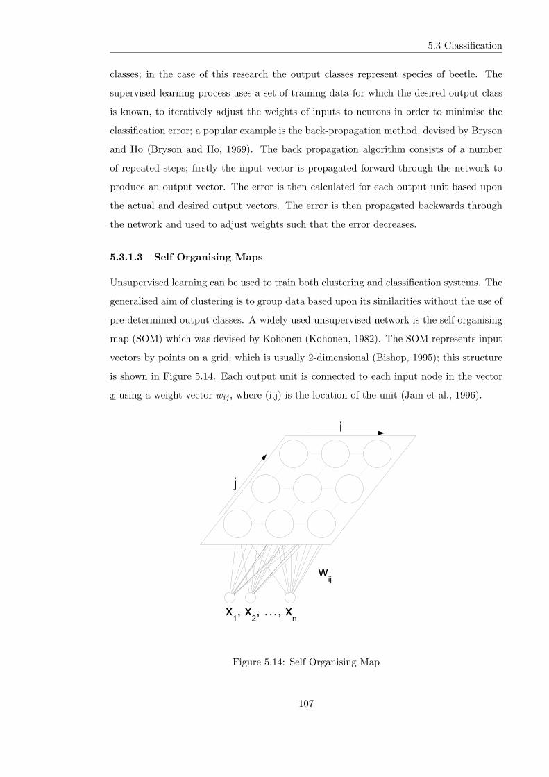
5.3 Classification
classes; in the case of this research the output classes represent species of beetle. The
supervised learning process uses a set of training data for which the desired output class
is known, to iteratively adjust the weights of inputs to neurons in order to minimise the
classification error; a popular example is the back-propagation method, devised by Bryson
and Ho (Bryson and Ho, 1969). The back propagation algorithm consists of a number
of repeated steps; firstly the input vector is propagated forward through the network to
produce an output vector. The error is then calculated for each output unit based upon
the actual and desired output vectors. The error is then propagated backwards through
the network and used to adjust weights such that the error decreases.
5.3.1.3 Self Organising Maps
Unsupervised learning can be used to train both clustering and classification systems. The
generalised aim of clustering is to group data based upon its similarities without the use of
pre-determined output classes. A widely used unsupervised network is the self organising
map (SOM) which was devised by Kohonen (Kohonen, 1982). The SOM represents input
vectors by points on a grid, which is usually 2-dimensional (Bishop, 1995); this structure
is shown in Figure 5.14. Each output unit is connected to each input node in the vector
x using a weight vector wij , where (i,j) is the location of the unit (Jain et al., 1996).
Figure 5.14: Self Organising Map
107

5.3 Classification
The learning algorithm begins by initialising all weights to random numbers. An input
vector is then selected at random from the data set and the distance from this vector to
all weight vectors is calculated. The Euclidean distance is commonly used and can be
calculated using equation 5.10, where yij is the distance to the unit at location (i,j) and
n is the number of dimensions in the input vector.
yij =
√
√
√
√
n∑
d=0
(xd − (wij)d)2 (5.10)
The winning or best matching unit is that which has the minimum distance to the
input vector. This unit is then used to calculate the neighbourhood of units which will
have their weights adjusted. A neighbourhood function decreases the neigbourhood size
with each training iteration, allowing the network to converge. The weights of units within
the neighbourhood are than updated using the rule shown in equation 5.11.
wij(t+ 1) = wij(t) + α(t)[x(t)− wij(t)] (5.11)
α(t) is the learning rate which is used to control the impact that input vectors have
on unit weights as training progresses; this value decreases with each iteration.
5.3.1.4 Learning Vector Quantization
Learning Vector Quantization (LVQ) is an ANN structure and training method which
combines elements of both supervised and unsupervised learning (Kohonen, 1990). This
is achieved by using two layers of neurons; an unsupervised layer which operates in similar
way to a SOM and clusters input vectors into sub-classes, and a linear layer which classifies
sub-classes into pre-defined output classes in a supervised manner.
108

5.3 Classification
Figure 5.15: LVQ Network
The network has two sets of weights; these are shown as w1 and w2 in figure 5.15. w1
weights connect input features to units in the competitive layer as with the SOM network.
w2 weights are used to map sub-classes to output classes.
In each training iteration an input vector is chosen and the best matching unit in the
competitive layer is calculated using equation 5.10. The output of this unit to the linear
layer is 1; all other competitive layer units will have output 0. If the input vector has been
classified correctly then the weight vector of the best matching unit is moved towards the
input vector using eqaution 5.12.
wij(t+ 1) = wij(t) + α(t)[x(t)− wij(t)] (5.12)
If the input vector has been classified incorrectly then the weight vector of the best
matching unit is moved away from the input vector using equation 5.13.
wij(t+ 1) = wij(t)− α(t)[x(t)− wij(t)] (5.13)
109

5.3 Classification
Various versions of LVQ exist (LVQ2, LVQ3) which attempt to overcome limitations
in the original LVQ algorithm (Kohonen, 1989), (Kohonen, 1995). However, a recent anal-
ysis of various versions of LVQ has suggested that the original method outperforms other
varients (Ghosh et al., 2006).
MLP networks trained with back propagation, and LVQ networks have been suggested
to be the most commonly used learning methods in pattern recognition (Frasconi et al.,
1997). Both MLP and LVQ have been sucessfully applied to several acoustic insect recog-
nition tasks and will be studied further.
5.3.1.5 Dimensionality
The term ’Curse of Dimensionality’ is often used to refer to problems encountered in using
high dimensional data. It was devised by Bellman and describes the exponential growth
of hypervolumes as a function of their dimension (Bellman, 1961). In neural networks
this means that the size of the training data set required to accurately train a network
increases exponentially with the dimensionality of the data.
In section 5.3.2.5 an MLP network is trained using data with dimensions varying
between 6 (for a tree depth of 2) to 126 (for a tree depth of 6). Whilst classification rates
increase when the data dimension is increased from 6 to 28, the small size of the data set
means that the larger network may in fact represent the data classes less well. A large
number of input features can lead to poor classifier generalisation if features are associated
with noise. Since the data set size is small, the network may be over representing irrelevent
portions of the input space.
5.3.2 Results
5.3.2.1 Neural Network Parameters
The MLP networks used have three layers: input, hidden and output. The number of
neurons in the hidden layer varies the number of input features and output classes and
is calculated using the equation given in section 5.3.2.5. The number of neurons in the
output layer is equal to the number of output classes. The value of each neuron’s output
is continuously variable and uses a unipolor sigmoid activation function. In each test the
network was trained through 500 iterations and a learning rate of 0.3 was used.
110

5.3 Classification
In the case of the LVQ networks, the number of units in the competitive layer varied
between 20 and 50. In each test the network was trained through 1000 iterations; an initial
learning rate of 0.1 and a linear decay learning function was used.
5.3.2.2 Data Sets
The two species of most interest to this project are A. glabripennis and A. chinensis (See
Chapters 2 & 3). Given the high quarantine status of these species, opportunities for
recording them are limited particularly since FERA did not obtain a licence for keep-
ing these species in its laboratories in York until the final year of this research when
A. glabripennis larvae were imported from France and several recordings of their feeding
were made. No opportunity has arisen to record any significant quantity of A. chinensis
feeding; therefore a substitute species, Hylotrupes bajulus has been used here. H. bajulus
is a wood-boring species native to the United Kingdom which is considered a pest as it
damages wood in buildings.
The A. glabripennis data set consists of 100 bites manually extracted from a number
of different recordings which are listed in Table 5.8.
Description Number of bites
Larva in live Acer, FERA, York 25th June 2010 34
Recording provided by FERA, March 2011 33
Recording provided by Massimo Faccoli (Italy), early 2011 33
Table 5.8: Anoplophora glabripennis recordings
The H. bajulus set consists of 100 bites manually extracted from a recording made by
Farr during the previous DEFRA project, ‘2005 06 30 CSL 30 June 2005 Hylotrupes Ba-
julus Block 005A 002.wav’ (Farr, 2007). The noise data set consists of 100 noise segments
extracted from recordings made in environments with no larvae present.
The A. planipennis set consists of 50 bites extracted from a recording provided by the
Canadian Food Inspection Agency which was made in an outdoor quarantine environment.
111

5.3 Classification
5.3.2.3 Generation of test data
Relational tree features were generated using custom software written in C♯. The inputs to
the software are bite audio data in the form of individual wave files which are grouped into
folders which represent species classes; and two parameters which define the tree depth
and amplitude quantization. The output of this software is a table of feature vectors for-
matted as a comma separated variable file which contains rows which represent each input
file and columns containing the feature vector and class identifier.
5.3.2.4 Cross Validation
The classification process was tested using Weka version 3.64 which is a data mining tool
implementing several machine learning techniques (Hall et al., 2009). MLP and LVQ
networks were testing using cross validation which is a method which avoids the need to
separate input data into a training and validation set. Data is divided into S segments
and the network trained using S − 1 of these segments; the unused segment is then used
to test the performance of the network (Stone, 1974). This process is repeated for all
S segments such that each is used for testing once and the classification error averaged
across S results. 10 segments were used for cross validation in all of the classification
results presented in this chapter.
5.3.2.5 Tree Depth Variation
An initial tree generation depth of four was selected and the largest number of amplitude
quantization levels (200) used. This produces an input vector consisting of 28 features. The
classification results of an MLP network with a single hidden layer of 15 neurons can be seen
in table 5.9 and correspond to an overall accuracy of 91.5%. The number of hidden layer
neurons uses the WEKA default calculation of n = (inputfeatures+ outputclasses)/2.
112

5.3 Classification
Classified as → A. glabripennis H. bajulus
A. glabripennis 90 10
H. bajulus 7 93
Confidence 0.928 0.903
Table 5.9: A. glabripennis vs. H. bajulus confusion matrix (Tree depth 4)
The depth of the tree generation was then varied and the classification process repeated
using the same set of data. The individual classification results can be seen in tables 5.10
to 5.13 and a summary in table 5.14.
Classified as → A. glabripennis H. bajulus
A. glabripennis 88 12
H. bajulus 18 82
Confidence 0.815 0.872
Table 5.10: A. glabripennis vs. H. bajulus (Tree depth 2)
Classified as → A. glabripennis H. bajulus
A. glabripennis 93 7
H. bajulus 11 89
Confidence 0.894 0.927
Table 5.11: A. glabripennis vs. H. bajulus (Tree depth 3)
Classified as → A. glabripennis H. bajulus
A. glabripennis 86 14
H. bajulus 10 90
Confidence 0.896 0.865
Table 5.12: A. glabripennis vs. H. bajulus (Tree depth 5)
113

5.3 Classification
Classified as → A. glabripennis H. bajulus
A. glabripennis 83 17
H. bajulus 9 91
Confidence 0.912 0.852
Table 5.13: A. glabripennis vs. H. bajulus (Tree depth 6)
Tree Depth Accuracy
2 85%
3 91%
4 91.5%
5 88%
6 87%
Table 5.14: A. glabripennis vs. H. bajulus Summary
As could be expected, performance decreases when a very shallow tree depth is used.
In this case the feature vector is too short and does not adequately represent the waveform.
The performance also decreases for very high values on tree depth which is perhaps due to
a larger proportion of features representing peaks which form parts of background noise,
leading to poor generalisation in the classifier. The results suggest that the optimum tree
depth is 4 layers.
5.3.2.6 Quantising amplitude values
One of the reasons for the selection of relational trees as a feature extraction method was
the ability to encode relative amplitude values. A set of tests was run in which the number
of quantization levels was varied, ultimately down to a single level to remove the feature
entirely, to determine whether relative amplitude information provides any advantage to
the classifier. The reduction in quantization levels is also potentially of interest since it
may allow the classifier to perform better at generalisation.
Figure 5.16 shows the classification results plotted against the number of amplitude
quantization levels using the same input data as the previous tests and a tree depth of 4.
114

5.3 Classification
This was repeated with the addition of a noise data class to produce the graph shown in
Figure 5.17. The full classification results of these tests can be seen in Appendix C.
Figure 5.16: Effect of quantization on A. glabripennis vs H. bajulus classification
Figure 5.17: Effect of quantization on A. glabripennis vs H. bajulus vs Noise classification
In classifying A. glabripennis and H. bajulus the peak classification accuracy is 92%
and is acheivable with 10 quantization levels. When no amplitude information is supplied
as a feature the accuracy decreases to 87%, showing that amplitude information does
improve classification. In classifying the two beetle species and noise the peak classification
115

5.3 Classification
accuracy, 91.67%, is acheived with 4 quantization levels and is significantly better than
the accuracy acheived when no amplitude information is used, at 79.67%.
5.3.2.7 LVQ vs. MLP
The results presented in the previous section all used an MLP neural network. In this
section the relative performance of LVQ and MLP networks is assessed.
LVQ classification between A. glabripennis and H. bajulus was first tested using 10
quantization levels and a tree depth of 4; the results can be see in Tables 5.15 to 5.18.
The number of LVQ first layer nodes is was varied from 20 to 50.
Classified as → A. glabripennis H. bajulus
A. glabripennis 92 8
H. bajulus 6 94
Confidence 0.939 0.922
Table 5.15: A. glabripennis vs. H. bajulus LVQ Results (20 first layer nodes)
Classified as → A. glabripennis H. bajulus
A. glabripennis 89 11
H. bajulus 3 97
Confidence 0.967 0.898
Table 5.16: A. glabripennis vs. H. bajulus LVQ Results (30 first layer nodes)
Classified as → A. glabripennis H. bajulus
A. glabripennis 93 7
H. bajulus 5 95
Confidence 0.949 0.931
Table 5.17: A. glabripennis vs. H. bajulus LVQ Results (40 first layer nodes)
116

5.3 Classification
Classified as → A. glabripennis H. bajulus
A. glabripennis 97 3
H. bajulus 4 96
Confidence 0.960 0.970
Table 5.18: A. glabripennis vs. H. bajulus LVQ Results (50 first layer nodes)
The results show that when 50 first layer nodes are used 96.5% of bites are correctly
classified, significantly higher than the 92% acheived using MLP.
Tables 5.19 to 5.22 show the results of classification between A. glabripennis, H. baju-
lus and noise using LVQ. Again the number of first layer nodes is varied between 20 and
50. When using 50 first layer nodes, LVQ performs better than MLP, correctly classifying
95.6% of inputs as opposed to 88.67% with MLP.
Classified as → A. glabripennis H. bajulus Noise
A. glabripennis 97 3 0
H. bajulus 4 94 3
Noise 7 4 88
Confidence 0.898 0.931 0.967
Table 5.19: A. glabripennis vs. H. bajulus vs. Noise LVQ Results (20 first layer nodes)
Classified as → A. glabripennis H. bajulus Noise
A. glabripennis 95 5 0
H. bajulus 2 96 3
Noise 5 4 90
Confidence 0.931 0.914 0.968
Table 5.20: A. glabripennis vs. H. bajulus vs. Noise LVQ Results (30 first layer nodes)
117

5.3 Classification
Classified as → A. glabripennis H. bajulus Noise
A. glabripennis 98 2 0
H. bajulus 2 97 2
Noise 4 4 91
Confidence 0.942 0.942 0.978
Table 5.21: A. glabripennis vs. H. bajulus vs. Noise LVQ Results (40 first layer nodes)
Classified as → A. glabripennis H. bajulus Noise
A. glabripennis 98 2 0
H. bajulus 2 92 2
Noise 4 3 92
Confidence 0.942 0.951 0.979
Table 5.22: A. glabripennis vs. H. bajulus vs. Noise LVQ Results (50 first layer nodes)
A final comparison between MLP and LVQ treated both species as a single class
to determine the performance of both classifiers at identifying bites from noise. The
classification results for MLP are shown in Table 5.23. LVQ results are shown in Tables
5.24 to 5.27.
Classified as → Bite Noise
Bite 196 5
Noise 8 91
Confidence 0.961 0.948
Table 5.23: Bite vs. Noise MLP Results
Classified as → Bite Noise
Bite 196 4
Noise 14 85
Confidence 0.933 0.955
Table 5.24: Bite vs. Noise LVQ Results (20 first layer nodes)
118

5.3 Classification
Classified as → Bite Noise
Bite 196 4
Noise 10 89
Confidence 0.951 0.957
Table 5.25: Bite vs. Noise LVQ Results (30 first layer nodes)
Classified as → Bite Noise
Bite 196 4
Noise 8 91
Confidence 0.961 0.958
Table 5.26: Bite vs. Noise LVQ Results (40 first layer nodes)
When using 50 first layer nodes, LVQ again outperforms MLP although the difference
is less than in the other classification tests. LVQ correctly classifies 96.66% of inputs
whereas MLP only correctly classifies 95.67%.
Classification between three species, A. glabripennis, H. bajulus and A. planipennis,
using LVQ was acheived with a lower overall success rate of 88.8%. The full results can
be see in Table 5.28.
Classified as → A. glabripennis A. planipennis H. bajulus
A. glabripennis 92 4 4
A. planipennis 7 37 6
H. bajulus 2 5 93
Table 5.28: A. glabripennis vs. A. planipennis vs. H. bajulus LVQ Results (50 first layer
nodes)
5.3.3 Classification of Unknowns
The classification methods adopted appear to perform well in distinguishing between a
small number of species but are not ideally suited to the detection of unknown inputs.
Unknowns may either be associated with a species for which the network has not been
trained, or with non-larvae sourced sounds such as those categorised as ’Noise’ in tables
119

5.4 Summary
Classified as → Bite Noise
Bite 197 3
Noise 7 92
Confidence 0.966 0.968
Table 5.27: Bite vs. Noise LVQ Results (50 first layer nodes)
5.19 to 5.27.
In a real-world environment the system is likely to encounter a wide range of ’unknown’
inputs which the neural networks adopted here could not be trained for since their features
may be significantly different. The ability of the system to deal with unknown inputs may
be necessary if the possible inputs cannot be limited by noise filtering and prior knowledge
of potential species. In this case a the use of a different classification method may be more
suitable.
5.4 Summary
This chapter has covered the species identification stage of the system. Several approaches
to feature extraction which have been used in the analysis of insect sounds have been dis-
cussed. A novel approach to extracting larval bite features, relational tree generation, has
been introduced.
The performance of two ANNs, MLP and LVQ, in classifying bites between two beetle
species and between bite and noise has been tested. The LVQ network has been found
to outperform MLP in each test case; classifying between A. glabripennis and H. bajulus
with 96.5% accuracy.
120

Chapter 6
System Implementation
This chapter covers the implementation of the larvae detection and identification tech-
niques described in the previous two chapters into a field deployable system for use by
PHSI and FC PHS inspectors. It begins by considering the implicit and explicit require-
ments for the detection system based upon the information provided by DEFRA in the
project proposal document and communication with PHSI inspectors who could poten-
tially use the system.
Section 6.2 details the methods used to manually record the activity of larvae before
the implementation of the automated system for the purpose of sensor testing and the
building of a larger library of larvae recordings. The hardware implementation of the
system is covered in section 6.3; this is separated into sensor design and implementation
and the selection of PC hardware. The software implementation is then covered in section
6.4 and is primarily described from the point of view of the features available rather than
being a full implementation report containing all of the underlying processes and code,
which are explained to a very limited extent.
The chapter concludes with a summary of the complete system as delivered to PHSI
and FC inspectors for field testing and feedback.
6.1 Requirements and Overview
The primary objective of the project, as defined by DEFRA is as follows:
121

6.1 Requirements and Overview
“To develop a real-time hand-held device (or alternative platform compatible with PH-
SI/FC equipment) capable of detection and identification of a range of taxa in hard plant
materials (including standing trees) for PHSI inspectors, and potentially FC inspectors, to
evaluate. To develop a real-time species detection and identification data logging system
for deployment and monitoring over an extended period of time. To develop a live insect
(non-specific) detection system.”
Any acoustic detection system, whether automated or manual, requires at least the
four stages shown in figure 6.1.
Figure 6.1: Components of a Detection System
The sound source is considered to be the combination of tree or wood sample with
unknown quantity and species of larvae inside; this has been discussed in chapter 3. DE-
FRA require two systems, a hand-held device and a data-logging device, both of which
will perform automated insect detection and identification. The specified and implied
requirements for these devices are set out in tables 6.1 and 6.2.
122

6.1 Requirements and Overview
Requirement Explicit Implicit
Real-time Detection •
Real-time Identification •
Non-destructive Attachement •
Robust (for outdoor use) •
Real-time output •
Compatible with PHSI/FC equipment •
Simple to operate, requiring no specialist knowledge
of underlying methods
•
Battery life suitable for field use •
Produce reliable results •
Sensors easily attachable and detachable •
Expandable •
Table 6.1: Hand-held System Requirements
Requirement Explicit Implicit
Automated Detection •
Automated Identification •
Non-destructive Attachment •
Weatherproof; suitable for prolonged periods of out-
door use
•
Output to storage •
Compatible with PHSI/FC equipment •
Simple to operate, requiring no specialist knowledge
of underlying methods and minimum user interaction
•
Battery life suitable for extended periods of field use •
Produce reliable results •
Sensors easily attachable and detachable •
Expandable •
Table 6.2: Data-logging System Requirements
The two systems share many of the same requirements; the only significant differences
between the two are in battery life requirements, user interface and whether real-time
123

6.2 Recording Equipment and Methods
analysis is required or not.
The data-logging system does not need to perform data analysis in real-time. In princi-
ple it could be based around a simple audio recorder which could store data to a removable
disk which could then be uploaded to a PC or other dedicated device for analysis. This
option was considered but was concluded to have several limitations; large amounts of
storage space are required since all recorded audio has to be stored for analysis. Perhaps
more significantly, the system would be unable to give any indication of the potential
presence of any infestation whilst in place since results would only be available to the user
after data was uploaded for analysis.
A decision was taken to focus on producing a single system which could be used as
both data-logger and hand-held device. No indication was provided by DEFRA or PHSI
as to the battery life requirements of either system nor how it was envisaged that such
a device were to be used. The limited information known about larval feeding behaviour
when inside wood also presented difficulties in specifying some aspects of the design. For
example, the presence of larvae does not imply the presence of detectable acoustic activity
since larvae don’t feed continuously. Therefore the longer a sample is monitored for, the
greater the chance of detecting any infestation which is present.
6.2 Recording Equipment and Methods
In the early stages of this project a number of recordings were made using simple piezo-
electric sensors in combination with hard disk and solid state disk based audio recording
devices. The purpose of this was two-fold; firstly it was used to test various aspects of
the sensor design and secondly it was used to build up a larger library of recordings. The
majority of these recordings were made within quarantine facilities with a limited number
being field recordings.
The recording devices used were the Edirol R4, Edirol R-09HR and the Marantz
PMD660. The Edirol R4 is a four channel hard disk based recorder which supports
sampling rates up to 96kHz with 16 or 24 bits per sample. The 40GB hard disk provides
enough storage space for 29 hours worth of recording when using four channels at 44.1kHz
with 16 bits per sample. It can be powered by either mains or batteries but both of these
124

6.2 Recording Equipment and Methods
options have limitations. Firstly, the batteries tended to run out very quickly, often lasting
little over an hour; secondly the mains power introduced a huge amount of mains noise
into the recordings. The R09HR and PMD660 are portable two channel devices which
record to secure digital (SD) and compact flash memory card respectively.
The sensors used were Kingstate KPEG116 piezoelectric transducers which were placed
inside plastic housings packed with foam and sealed closed. The piezoelectric transducers
were held in place only by the pressure of the layers of foam padding; no glue was used.
Figure 6.2 shows the side view of the sensor construction.
Figure 6.2: Side view of encased sensor
The method of attaching the sensor was dependent on the size of the sample. Rubber
bands were used on small tree trunks and pieces of timber while rubber tree straps were
used for larger standing trees. Sensors in place attached to samples using both methods
can be seen in Figures 6.3 and 6.4.
125

6.3 Hardware Implementation
Figure 6.3: Sensor attached using a tree strap
A number of ‘speculative’ recording sessions were undertaken throughout the course
of the project. These involved making recordings of samples which came from potentially
infested shipments of material or trees but where the infestation status of the individual
samples was unknown. These proved to be of little use to the project since the detection of
activity was very rare; this could be attributed to the lack of infestation or activity, or due
to poor performance of the detection system. The manual processing of the resultant audio
data was required and more often than not the cause was lack of larval activity. Towards
the end of the project, FERA obtained a number of live Anoplophora glabripennis larvae
which were placed inside inside tree stumps to allow the system to be tested with known
infested material. A full list of the recordings made during this project is provided in
Appendix D.
6.3 Hardware Implementation
6.3.1 Sound Cards and USB Sensors
It is very uncommon for a PC, hand-held or otherwise, to have no inbuilt sound card. A
sound card is a device which provides a PC with the capability to output and/or input au-
126

6.3 Hardware Implementation
Figure 6.4: Sensor attached using rubber bands
dio, usually both. Most sound cards provide at least analogue microphone input, analogue
line level input and analogue loudspeaker output with many also featuring digital input
and output (SPDIF - optical, composite or both) and various other analog outputs for
surround-sound systems. These devices tend to follow, sometimes loosely, Intel’s Audio
Codec 97 specifications, now at revision 2.3 (Intel, 2002). Table 65 of the specification
document lists various analogue performance characteristics, those relevant to this project
are reproduced here in table 6.3.
Parameter Minimum Typical Maximum Units
Full Scale Input (Microphone) - 0.1 - Vrms
Full Scale Input (Line Level) - 1.0 - Vrms
Analogue Frequency Response 20 - 20,000 Hz
Input Impedance 10 - - kΩ
Input Capacitance - 7.5 - pF
Input Channel Crosstalk - - -70 dB
Table 6.3: Selection of AC ’97 Analogue performance characteristics
127

6.3 Hardware Implementation
It was initially envisaged that the sensors would be directly connected to the analogue
microphone input of whichever integrated sound card was fitted. Early testing uncovered
several potential issues with this approach for which various solutions were considered;
these are summarised below.
1. When the PC was accessing the hard disk significant levels of noise were introduced
to the input channels of the sound device. An external sound device or analogue to
digital converter could be used to eliminate this type of noise.
2. There are variations between sound cards in different PCs which could affect the
recordings made with them. Whilst this would not be an issue if a single type of
hand-held PC was being used, during development the sensors were used with various
machines and for convenience the elimination of any variation was preferable.
3. The use of an integrated sound card would limit the system to using a maximum of
two sensors at any one time. If one of the channels is used for an ambient sound
sensor then only one sample sensor could be used. ‘Time slicing’ could be used to
connect multiple sensors per channel, alternatively USB connection could be used
which would increase the potential number of concurrently attached sensors.
4. The requirement of an analogue audio input limits the potential choice of hand-held
PC’s since several do not have this type of connection, instead having integrated
microphones which are not suitable for use in the recording of larvae.
5. There is a risk of user error associated with using analogue audio input since identical
jacks are used for line-level input, headphone output and various surround-sound
outputs.
6. The sensors will require a pre-amplifier. The power source for this will either need
to be a battery built into the sensor, microphone phantom power from the sound
card or from a USB port.
7. Various configuration options relating to the default sound card on a Windows ma-
chine tend to change without warning. Gain levels in particular seem to be particu-
larly susceptible to this.
128

6.3 Hardware Implementation
The combination of these issue led to the development of a new sensor which combines
a USB audio circuit with in-built amplification. These units make use of the two audio
channels available by the addition of a secondary sensor which is used to detect acoustic
events which are not produced by larvae, to reduce the rate of false positive detections.
An overview of the sensor design can be seen in Figure 6.5.
Figure 6.5: USB Dual Sensor Design
These sensors provide recordings which are independent of the PC hardware to which
the sensor is connected. An additional benefit is that the bite detection software is able to
monitor for the presence of attached sensors and produce warnings when they are removed.
6.3.2 Hand-held PCs and embedded devices
The hand-held PC is a standard ‘off the shelf’ product, the Samsung Q1. This was selected
as a prototype based upon its comparatively long battery life and availability of low cost
ruggedised cases which are essential for its use in a field environment.
PC hardware improves rapidly over time and it is very likely that a more suitable
device is now available. Any future version of the system would ideally have better specified
requirements by FERA which may result in a significantly different hand-held device being
used.
129

6.4 Software Implementation
6.4 Software Implementation
This section is intended to serve as an overview of the software’s capabilities and basic
structure rather than a full implementation report. The detection software is capable of
fully automated real-time analysis when capturing sound directly from an attached sensor.
It can also perform non-real-time or simulated real-time analysis of imported recordings
stored as audio files. It is written in Microsoft C♯ and requires the .NET Framework 2.0
and Direct X Direct Sound library and is therefore dependent on the windows platform;
an overview of the software is provided in Figure 6.6.
130

6.4Softw
areIm
plem
entation
Figure 6.6: Software Overview
131

6.4 Software Implementation
6.4.1 Inputs
The first stage in the software is the selection of an audio source which will be analysed.
At the request of FERA, the software allows multiple types of input audio source to be
used in addition to the recommended USB sensors.
1. Mono Audio File A prerecorded audio file can be opened for analysis. This can
optionally be run through the system in ‘real-time’ to simulate the presence of an
attached sensor. Any saved events such as bite audio files or species results are
time-stamped with their position within the original file.
2. Stereo Audio File As for mono audio files except that a second channel is provided
as the ambient sound, or control, source. The channel providing containing ambient
sound can be selected so that the system can cope with recordings which have been
made with the sensor channels swapped.
3. USB Sensor This tells the software to record audio from an attached USB sensor
and is the suggested method of using the system. If no sensor is attached to the
PC this option is not enabled. The USB sensors record two channels, one for the
subject, one for ambient sound. The channels used for these sensors are fixed since
the user cannot physically switch them around.
4. Sound card input The option to allow the use of a built in PC sound card was
added at the request of FERA. As has been discussed earlier in this chapter, internal
PC sound cards are not well suited for use in a system such as this and this input
method is therefore not recommended.
The expected input format is uncompressed pcm audio data sampled at 44.1kHz with
16 bits per sample. If a USB sensor or internal sound input is being used the software
will attempt to initialise the audio device with these parameters which are supported by
the vast majority of PC sound devices. If the input source being used is an audio file the
software will expect a file in WAVE format with the above parameters. Sampling rates
other than 44.1kHz are supported but the fractal analysis frame size must be adjusted
accordingly since it is measured in samples rather than seconds.
132

6.4 Software Implementation
6.4.2 Detection
In this section the event detection aspect of the software will be discussed. This task can
be considered independently of the other functions of the software since the analysis is
performed linearly on fixed input data to produce a single set of outputs. The input to
the detection stage is a segment of mono audio data, if a single sensor is being used, or
stereo data if an ambient sensor is also attached.
Figure 6.7: Detection Process
133

6.4 Software Implementation
Incoming audio data from either sensors or a WAVE file is provided to the bite detector
in segments which are one second in length. This length is used to allow the system to
provide a near-realtime indication of any detection whilst also being of sufficient length to
enable the average based thresholding used by the detection method to operate.
For each segment, the fractal dimension detection method described in chapter 4 is
used to generate a list of frames and their respective detection results (either ones or
zeros). Given a frame size of 300 samples, the example frame list results shown in table
6.4 correspond to a single event positioned at between 1500 and 2100 samples in the audio
segment.
Frame Position Detection (0 = No, 1= Yes)
0 0
1 0
2 0
3 0
4 0
5 1
6 1
7 1
8 0
9 0
10 0
Table 6.4: Example Frame Results Table
If two sensors are present the detection results for all fractal dimension frames within
the audio segments are compared. Any frames which have been registered as containing
an event from the ambient channel are set to zero in the primary channel. This means
the output event list only contains events which have been registered exclusively in the
primary sensor channel. Table 6.5 is a truth table for this operation.
134

6.4 Software Implementation
Primary Sensor Event List Ambient Sensor Event List Output Event List
0 0 0
0 1 0
1 1 0
1 0 1
Table 6.5: Events List Truth Table
A list of events including start and end positions, in samples, is produced. Events
which are located very closely together are merged and events which exceed a predefined
maximum event length are excluded. The list of detected events is then passed to the
classification stage and optionally stored as individual audio files.
6.4.3 Identification
The identification stage takes as its inputs the list of detected events as produced by the
detection stage, and the original audio segment data. The classification process is visu-
alised in Figure 6.8.
Figure 6.8: Bite Identification Process
135

6.4 Software Implementation
The relational tree generation feature extraction method and LVQ neural network de-
scribed in Chapter 5 are used to classify bite species. Once all detected events have been
classified the results are displayed on screen and optionally written to the hard disk.
The version of the software which was supplied to DEFRA did not have the bite
identification stage enabled.
6.4.4 Threading
The software makes use of three threads which allow it to perform real-time analysis whilst
simultaneously recording new data and keeping the user interface updated with results.
The primary duties of, and communication between these threads can be seen in Figure 6.9.
Figure 6.9: Threads
When the software is first started only a single thread, the main thread, is active.
This controls and updates the user interface and starts other threads in response to user
input. When the user instructs the software to start recording, the recording thread is
136

6.5 Complete System
started; subject to the successful initialising of the requested sound device. The recording
thread then runs continuously alongside the main thread capturing audio from the sound
device and reporting back when new audio data is available for analysis until it receives
an instruction to stop. The main thread starts a new instance of the analysis thread each
time new audio data is available. This then analyses the segment of audio data before
returning results to the main thread before terminating itself.
6.4.5 System Output and Data Storage
Data collected at each of the stages shown in Figure 6.1, recording, detection and iden-
tification, can be stored for later use. At the recording stage this is in the form of a
single WAVE audio file containing unmodified data as captured by the USB sensor(s). At
the detection stage, events which exceed the required threshold are stored individually as
WAVE audio files with time stamps indicating when they were detected. At the identifi-
cation stage the species, if any, of detected events can be stored along side a time stamp
for the event.
6.4.6 Limitations
The software is limited to supporting a maximum of two attached sensors; one for attach-
ing to samples and the other to capture ambient sound. The underlying code is capable
of supporting a greater number of sensors and this support could be enabled if needed by
PHSI subject to suitable testing being carried out to determine the upper limit attached
sensors.
The maximum file size which can be loaded for analysis is 512MB as larger files produce
‘out of memory’ errors. This can be overcome by the use of a more efficient file loading
routine.
6.5 Complete System
The complete system delivered to PHSI for testing consisted of the following:
Hand-held PC
• Samsung Q1 Ultra Portable PC
137

6.6 Summary
• 40GB hard-disk storage (capable of storing over 3,000,000 bites)
• Operating System: Microsoft Windows XP Tablet Edition
• 4AH battery (providing around 8 hours continuous usage)
• Cost per unit £400
• Acoustic bite detection software installed
Acoustic Sensors
• Dual sensor system
• Piezo-electric transducer sensors in plastic ABS casings
• USB Audio using Texas Instruments PCM2902 chips
• Audio pre-amplifiers providing a gain of 20
Peli-Case
• Large shock-proof case containing the above items in addition to:
• Stereo headphones
• Rubber tree straps for attaching sensors
• Power adaptor for hand-held PC
6.6 Summary
In this chapter the requirements for the hand-held and data-logging systems as defined by
DEFRA were considered. The generalised requirements for an acoustic detection system
were discussed in addition to the specific requirements of the two automated systems. The
recording methods used before the development of the automated system were discussed
along with the initial designs of the sensors used in these recording sessions.
The hardware implementation of the system including the use of USB attached sensors
with built in pre-amplification was then detailed in section 6.3. Section 6.4 provided an
overview of the software implementation including methods of input, analysis and output
to storage and display. Finally the complete system as supplied to PHSI for testing was
described in section 6.5.
138

6.6 Summary
Figure 6.10: Complete System
139

Chapter 7
Conclusions and Further Work
7.1 Conclusions
Invasive Non-Native Species are a constant threat to the U.K. environment and economy.
A group of species which are of particular concern to DEFRA at present are wood-boring
beetles. These insects spend a high proportion of their life-cycles as larvae inside timber
and trees and are therefore difficult to detect.
Current detection techniques employed by PHSI inspectors rely on visual inspection
such as looking for beetle exit holes or frass; and manual destructive sampling. Visual
inspection may not provide a reliable indication of infestation, particularly if no adults
have emerged from a sample; destructive sampling is a time consuming process and may
not be financially viable for consignments of high value plants. DEFRA are therefore
interested in the development of techniques to detect larvae in a non-destructive manner.
The stated purpose of this project is “to aid the work of the Plant Health and Seeds
Inspectors (PHSI) and Forestry Commission (FC) inspectors by improving their ablity to
detect a range of statutory/quarantine pests using the acoustic methods initially investi-
gated in a previous Plant Health Division funded project PH0191, which established proof
of principle” (DEFRA, 2007).
The piezo-electric sensors used in the previous project (PH0191) were tested and their
performance relative to new low cost accelerometer based sensors was investigated. It was
concluded that the accelerometer based sensors provide no significant advantage over the
140

7.2 Evaluation of the adopted system
piezo-electric sensors and are more expensive to produce, more complex and more diffi-
cult to acoustically couple with sample material; their suitability was therefore discounted.
A low cost (both computationally and economically) dual sensor method has been sug-
gested in order to further reduce the rate of false positive detections. These incorporate
USB audio and amplification circuitry which enable recordings to be made with consis-
tent characteristics and gain which is independent of the PC hardware to which they are
connected. The use of a new technique for bite event detection, Fractal Dimension (FD)
detection, has been introduced in Chapter 4 and it has been shown to perform significantly
better than short time energy detection for events with low signal to noise ratios. At a
signal to noise ratio of 2, the difference from the mean value in fractal dimension for bites
is 6.61, compared to an equivalent short time energy difference of 2.03. This advantage
enables fractal dimension detection to be used to detect bites at lower signal to noise ratios.
Limitations in the use of TDSC as a feature extraction method for bite waveforms
have been demonstrated and a novel method for the extraction of features from bite
sounds based upon relational tree structures has been developed. The performance of this
method in combination with Multilayer Perceptron and Linear Vector Quantisation neural
networks has been assessed in Chapter 5.
Classification between two species, A. glabripennis and H. bajulus has been achieved
with rates of 92% using MLP and 96.5% using LVQ networks. Classification between the
two species and noise has been achieved with rates of 88.7% using MLP and 95.6% using
LVQ. Classification between three species A. glabripennis, A. planipennis and H. bajulus
has been achieved with a rate of 88.8% using an LVQ network.
The detection and identification methods developed here have been implemented in
a prototype real-time hand-held PC based system which has been supplied to FERA for
further testing.
7.2 Evaluation of the adopted system
The system can provide a real-time indication of potential larval activity, however if all
larvae in the sample are not feeding the system will provide a false negative result. With-
141

7.2 Evaluation of the adopted system
out extensive behavioural study of larvae it is impossible to quantify the confidence in any
real-time detection result since the percentage of time a larva spends feeding is unknown.
The longer the system can be attached to each sample, the greater the likelihood of de-
tecting any larval infestation. Until data on the feeding behaviour of larvae is obtained,
the time required to accurately analyse each sample cannot be calculated. The use of the
detection and identification methods developed may best suited to long term monitoring
of host plants.
The number of species which the system can identify is currently very low; the species
classification aspect of system in it’s current state has limited practical usefulness. In
order to scale up the system to perform identification of a wider range of species the clas-
sification method used may require significant alteration. The classification rates achieved
for three species detection were lower than those for two species. It is likely that if the
neural network was trained with additional species, the classification rate would decrease
further. If larger data sets could be obtained for each of the species it is possible that
classification rates may be attained by changing the topology of the neural networks by,
for example, increasing the number of neurons.
It is very unlikely that the system could be scaled up indefinately to cope with the
identification of all possible species of beetle without the use of prior knowledge such as
tree species or location within the tree. It is however, unlikely that a situation would arise
in which the system would be required to classify a large number of species.
The hardware and software system produced and supplied to FERA can be consid-
ered to be a prototype rather than a final system. Very little information was provided
regarding specification requirements such as battery life, species range and deployment
environment. Several software and hardware design decisions reflect the lack of specifica-
tion from FERA and were taken to make the system as flexible as possible. The software
was written in C♯ to allow it to run on most modern desktop and laptop PCs whilst also
being simple to port to Windows based embedded PCs, handhelds or even mobile phones.
The PC hardware, the Samsung Q1, was selected primarily for it’s long battery life of up
to 10 hours. Sensors were produced with embedded sound cards and USB connectivity to
ensure that they would be compatible with other PC hardware.
142
7.3 Further Work
If the system requirements were strictly specified by FERA and sufficient supplies
of larvae were available for the generation of a large library of feeding sounds, both the
hardware and software used in the system would likely change significantly from the current
design.
7.3 Further Work
7.3.1 Beetle Species Range
The results presented in this thesis have been limited to a small number of beetle species
due to the difficulty in obtaining known infested material, particularly where the desired
species is an INNS. In order for the species identification aspect of the system to be of real
practical use, the range of species which can be classified needs to be expanded. It is not
currently known how well the classification methods would perform with a large range of
species.
The methods here could be combined with additional information which could assist
classification such as the sample species, geographic information or time of year. Infor-
mation such as this could be used to produce a knowledge based system which would be
able to partition the classification space based upon prior knowledge of the likelihood of
certain species being present.
7.3.2 More Recordings
This research has been limited by the availability of known infested material which can be
recorded; access to quarantine species for recording is for obvious reasons rather difficult.
The methods and system developed could be improved based upon information obtained
from a much larger set of recordings. This would also enable the classification techniques
to be further validated.
A large set of recordings made in varied environments may also provide useful infor-
mation relating to the biological study of the species such as host preferences.
143

7.3 Further Work
7.3.3 Behavioural Study
There is still relatively little known about the feeding behaviour of beetle larvae in wood.
The detection methods developed here could be used to produce and analyse recordings of
a wider range of species over long time-periods. This would enable a greater understanding
of how feeding is effected by various external and internal factors. For example, anecdotal
evidence was obtained during the course of this research that larvae may be sensitive to
the sudden movement of their host material (See Chapter 4) and that the rate of feeding
activity may be related to the time of day.
Behavioural information could then be used to improve the performance of a detection
system either by utilising this knowledge within the system itself or by adjusting the way
that it is used in order to maximise the likelihood of detection.
7.3.4 Wireless Sensor Networks
The techniques developed here could be extended to a large scale network of sensors, used
to monitor greater numbers of trees over long time periods. Such a network may be of
particular use in conjunction with sentinel trees when used to monitor the spread of in-
festations or to monitor consignments of imported trees during post import growth.
It has been shown in Section 5.2.5 that the relational tree feature extraction method
represents bite audio data in a significantly compressed format. This could be exploited in
a wireless sensor network since feature data could be transmitted to a central classification
system using low bandwidth data links.
7.3.5 Native Species
The research undertaken so far has concentrated on the detection and identification of
non-native species. The methods here could be used to detect native wood-boring species
and may be suited to applications in the area of preservation of wood in listed buildings.
Piezo-electric sensors similar to those used in this research are currently being used in the
non-invasive monitoring of stag beetles (Lucanus cervus) (Harvey et al., 2011).
144

Appendix A
Publication List
Schofield, J. & Chesmore, D. (2008) Automated acoustic identification of beetle larvae in
imported goods using time domain analysis. Proceedings of Acoustics 2008, Paris, June
2008, 5929-5934.
Chesmore, D. & Schofield, J. (2009) Developing acoustic detection and identification meth-
ods for Anoplophora spp. Second International Symposium on Anoplophora chinensis and
A, glabripennis: Phytosanitory Strategies and Research, Vertemate Con Moniprio, Como,
Italy, 1-3 April 2009.
Schofield, J . & Chesmore D. (2010) Automated identification of beetles in hardwood. Royal
Entomological Society Technological Special Interest Group, Harpenden, 13 May 2010.
Schofield, J. & Chesmore D. (2010) Acoustic detection and monitoring of wood boring
beetles. Entomology 2010, Swansea, 26-28 July 2010.
Chesmore, D. & Schofield, J. (2010) Acoustic detection of statutory pests in hardwood
material. Bulletin of the European Plant Pathology Organisation (EPPO).Vol. 40(1),
46-51.
145

Appendix B
Fractal Dimension C# Code
stat ic double [ ] s e v c i k f r a c t a l ( short [ ] data , int f rame length )
double ymax = 0 , ymin = 0 , length , d , y current , y o ld ;
int s t a r t f r ame pos , end frame pos ;
double [ ] d array = new double [ data . Length/ f rame length ] ;
for ( int frame=0; frame<(data . Length/ f rame length ) ; frame++)
l ength = 0 ;
y cur r en t = 0 ;
y o ld = 0 ;
s t a r t f r ame po s = ( frame ∗ f rame length ) ;
end frame pos = ( frame ∗ f rame length ) + frame length ;
ymin = ymax = data [ s t a r t f r ame po s ] ;
for ( int i = s t a r t f r ame po s +1; i<end frame pos ; i++)
i f ( data [ i ] < ymin ) ymin = data [ i ] ;
i f ( data [ i ] > ymax) ymax = data [ i ] ;
146

y o ld = ( data [ s t a r t f r ame po s ] − ymin ) / (ymax − ymin ) ;
for ( int i = s t a r t f r ame po s +1; i<end frame pos ; i++)
y cur r en t = ( data [ i ] − ymin ) / (ymax − ymin ) ;
l ength += Math . Abs ( y cur r en t − y o ld ) ;
y o ld = y cur r en t ;
d = 1 + Math . Log ( l ength ) / Math . Log (2 ∗ ( f rame length − 1 ) ) ;
d array [ frame ] = d ;
return d array ;
147

Appendix C
Additional Classification Results
Classified as → A. glabripennis H. bajulus
A. glabripennis 90 10
H. bajulus 6 94
Confidence 0.938 0.904
Table C.1: A. glabripennis vs. H. bajulus MLP, Depth 4, Quantization 200 levels
Classified as → A. glabripennis H. bajulus
A. glabripennis 90 10
H. bajulus 6 94
Confidence 0.938 0.904
Table C.2: A. glabripennis vs. H. bajulus MLP, Depth 4, Quantization 100 levels
Classified as → A. glabripennis H. bajulus
A. glabripennis 89 11
H. bajulus 6 94
Confidence 0.937 0.895
Table C.3: A. glabripennis vs. H. bajulus MLP, Depth 4, Quantization 50 levels
148

Classified as → A. glabripennis H. bajulus
A. glabripennis 89 11
H. bajulus 6 94
Confidence 0.937 0.895
Table C.4: A. glabripennis vs. H. bajulus MLP, Depth 4, Quantization 20 levels
Classified as → A. glabripennis H. bajulus
A. glabripennis 91 9
H. bajulus 7 93
Confidence 0.929 0.921
Table C.5: A. glabripennis vs. H. bajulus MLP, Depth 4, Quantization 10 levels
Classified as → A. glabripennis H. bajulus
A. glabripennis 92 8
H. bajulus 10 90
Confidence 0.902 0.918
Table C.6: A. glabripennis vs. H. bajulus MLP, Depth 4, Quantization 4 levels
Classified as → A. glabripennis H. bajulus
A. glabripennis 92 8
H. bajulus 10 90
Confidence 0.902 0.918
Table C.7: A. glabripennis vs. H. bajulus MLP, Depth 4, Quantization 2 levels
Classified as → A. glabripennis H. bajulus
A. glabripennis 94 6
H. bajulus 20 80
Confidence 0.825 0.930
Table C.8: A. glabripennis vs. H. bajulus MLP, Depth 4, Quantization 1 level
149

Classified as → A. glabripennis H. bajulus Noise
A. glabripennis 88 10 1
H. bajulus 8 89 4
Noise 4 4 91
Confidence 0.880 0.864 0.948
Table C.9: A. glabripennis vs. H. bajulus vs. Noise MLP, Depth 4, Quantization 200
levels
Classified as → A. glabripennis H. bajulus Noise
A. glabripennis 90 9 1
H. bajulus 7 90 4
Noise 4 5 90
Confidence 0.891 0.865 0.947
Table C.10: A. glabripennis vs. H. bajulus vs. Noise MLP, Depth 4, Quantization 100
levels
Classified as → A. glabripennis H. bajulus Noise
A. glabripennis 89 10 1
H. bajulus 8 89 4
Noise 4 4 91
Confidence 0.881 0.864 0.948
Table C.11: A. glabripennis vs. H. bajulus vs. Noise MLP, Depth 4, Quantization 50
levels
150

Classified as → A. glabripennis H. bajulus Noise
A. glabripennis 90 9 1
H. bajulus 10 87 4
Noise 4 4 91
Confidence 0.865 0.870 0.948
Table C.12: A. glabripennis vs. H. bajulus vs. Noise MLP, Depth 4, Quantization 20
levels
Classified as → A. glabripennis H. bajulus Noise
A. glabripennis 88 10 2
H. bajulus 8 87 6
Noise 4 4 91
Confidence 0.880 0.847 0.919
Table C.13: A. glabripennis vs. H. bajulus vs. Noise MLP, Depth 4, Quantization 10
levels
Classified as → A. glabripennis H. bajulus Noise
A. glabripennis 88 9 3
H. bajulus 3 93 5
Noise 2 3 94
Confidence 0.946 0.809 0.922
Table C.14: A. glabripennis vs. H. bajulus vs. Noise MLP, Depth 4, Quantization 4 levels
Classified as → A. glabripennis H. bajulus Noise
A. glabripennis 83 13 4
H. bajulus 10 84 7
Noise 3 5 91
Confidence 0.865 0.824 0.892
Table C.15: A. glabripennis vs. H. bajulus vs. Noise MLP, Depth 4, Quantization 2 levels
151

Classified as → A. glabripennis H. bajulus Noise
A. glabripennis 65 33 2
H. bajulus 12 83 6
Noise 4 4 91
Confidence 0.802 0.692 0.919
Table C.16: A. glabripennis vs. H. bajulus vs. Noise MLP, Depth 4, Quantization 1 level
152

Appendix D
Recordings made during this
project
Date Location Samples Duration
20.02.09 CSL Quarantine Lab 1x Headboard pest 30 Mins
13.03.09 CSL Quarantine Lab 1x Headboard pest 24 Hours
06.04.09 Assago, Milan, Italy 3 trees infested with A. chinensis 2 Hours
01.06.09 CSL Quarantine Lab 1x mini-Acer 24 Hours
18.06.09 CSL Quarantine Lab 3x mini-Acer, 1 x wooden bowl 24 Hours
23.03.10 CSL Quarantine Lab Wooden post infested with Monochamus
galloprovincialis
24 Hours
02.06.10 National Refer-
ence Laboratory,
Netherlands
Acers inoculated with A. chinensis 2 Hours
24.06.10 Kew Gardens Various 1 Hour
25.06.10 CSL Quarantine Lab 4x Acers and Poplars with A. glabripennis 24 Hours
14.07.10 CSL Quarantine Lab 4x Acers and Poplars with A. glabripennis 24 Hours
07.10.10 CSL Quarantine Lab 4x Acers and Poplars with A. glabripennis 24 Hours
12.10.10 CSL Quarantine Lab 4x Acers and Poplars with A. glabripennis 24 Hours
20.10.10 CSL Quarantine Lab 4x Acers and Poplars with A. glabripennis 24 Hours
Table D.1: List of recordings made during this project
153

Appendix E
Recordings made by others
Source Location Species Details
Previous Project
PH0109 [Farr, 2007]
CSL Quarantine Lab,
York
H. bajulus File: 2005 06 30
CSL 30 June 2005
Hylotrupes Bajulus
Block 005A 002.wav
FERA FERA Quarantine
Lab, York
A. glabripennis Recordings made
during March 2011
Universita Degli
Studi Die Padova,
Italy
Italy A. glabripennis Recordings made
early 2011
Canadian Food In-
spection Agency
Outdoor Quarantine
facility, Canada
A. planipennis
Table E.1: List of recordings made by others
154

References
I. Adachi. Reproductive biology of the white-spotted longicorn beetle,
Anoplophora malasiaca (Thomson) (Coleoptera: Cerambycidae), in citrus
trees. Applied Entomology and Zoology, 23:256–264, 1988.
I. Adachi. Development and life cycle of Anoplophora malasiaca (Thomson)
(Coleoptera Cerambycidae on Citrus trees under fluctuating and constant
temperature regimes). Applied Entomology and Zoology, 29(4):485–497, 1994.
M. A. Al-Manie and M. I. Alkanhal. Acoustic Detection of the Red Date Palm
Weevil. World Academy of Science, Engineering and Technology, 2:160–163, 2005.
R. D. Alexander. Sound Production and Associated Behavior in Insects. The
Ohio Journal of Science, 57(2):101–113, 1957.
R. D. Alexander and T. E. Moore. Studies on the Acoustical Behavior of Seventeen-
Year Cicad. The Ohio Journal of Science, 58(2):107–127, 1958.
K. Antal. The investigation of applicability of acoustic emission technology for
the assessment of mechanical properties of wood. PhD thesis, Univeristy of West
Hungary, 2004.
A. C. Anulewicz, D. G. Mccullough, D. L. Cappaert, and T. M. Poland. Host Range
of the Emerald Ash Borer (Agrilus planipennis Fairmaire) (Coleoptera:
Buprestidae) in North America: Results of Multiple-Choice Field Exper-
iments. Environmental Entomology, 37(1):230–241, 2008.
R. E. Apfel. Ultrasonics. Methods of experimental physics, chapter Acoustic cavi-
tation, page 356. Academic Press, New York, 1981.
APHIS. Asian Longhorned Beetle (Anoplophora glabripennis) Factsheet. Online
155

REFERENCES
at ”http://www.aphis.usda.gov/publications/plant health/content/printable version/-
faq ALB Jan 05.pdf”, 2005a.
APHIS. Asian Longhorned Beetle: Questions and Answers. Online at
”http://www.aphis.usda.gov/publications/plant health/content/printable version/faq
alb 07.pdf”, May 2007.
APHIS. Emerald Ash Borer The Green Menace. Online at:
http://www.aphis.usda.gov/publications/plant health/content/printable version/EAB-
GreenMenace-reprint-June09.pdf, 2009.
USDA APHIS. Program for Biological Control of Saltcedar (Tamarix spp.) in
Thirteen States. Fort Collins, Colorado, 2005b.
J. Ayarkwa. Comparing the Effectiveness of Three Acoustic Emission Proce-
dures for Predicting Strengths of Finger-Joints from Tropical African Hard-
woods. Ghana Journal of Forestry, 26:1–13, 2010.
W. J. Bell, L. M. Roth, and C. A. Nalepa. Cockroaches: ecology, behavior, and
natural history. Johns Hopkins University Press, 2007.
R. Bellman. Adaptive Control Processes: A Guided Tour. Princeton University
Press, 1961.
U. Benker, C. Bogel, and M. Blaschke. Tree fellings due to black longicorn beetle:
the asiatic longicorn beetle has been found in the district of Passau [Bavaria,
Germany]. Allgemeine Forst Zeitschrift fur Waldwirtschaft und Umweltvorsorge, 59
(20):1112, 2004.
H. Bennet-Clark. Tymbal mechanics and the control of song frequency in the
cicada Cyclochila australasiae . Journal of Experimental Biology, 200(11):1681–
1694, 1997.
F. Bimbot, J. Bonastre, C. Fredouille, G. Gravier, I. Magrin-Chagnolleau, S. Meignier,
T. Merlin, J. Ortega-Garcia, D. Petrovska-Delacretaz, and D. A. Reynolds. A Tutorial
on Text-Independent Speaker Verification. EURASIP Journal on Applied Signal
Processing, 4:430–451, 2004.
156

REFERENCES
P. Binggeli. Misuse of terminology and anthropomorphic concepts in the de-
scription of introduced species. Bulletin of the British Ecological Society, 25:10–13,
1994.
M. C. Birch and J. J. Keenlyside. Tapping Behavior Is a Rhythmic Communication
in the Death-Watch Beetle, Xestobium rufovillosum (Coleoptera: Anobi-
idae). Journal of Insect Behaviour, 4(2):257–263, 1991.
C. Birnbaum. NOBANIS - Invasive Alien Species Fact Sheet - Mustela vision. -
From Online Database of the North European and Baltic Network on Inva-
sive Alien Species - NOBANIS www.nobanis.org, Date of access 31/01/2011,
2006.
C. M. Bishop. Neural Networks for Pattern Recognition. Oxford University Press,
1995.
L. Bonesi and S. Palazon. The American mink in Europe: Status, impacts, and
control. Biological Conservation, 134:470–483, 2007.
M. Borghetti, A. Raschi, and J. Grace. Ultrasound acoustic emission in water-
stressed plants of Picea abies Karst. Annals of Forest Science, 46(Supplement):
346–349, 1989.
C. K. Brain. Preliminary note on the adaptation of certain radio principles to
insect investigation work. Ann. Univ. Stellenbosch, 2:45–47, 1924.
O. Breidbach. Studies on the Stridulation of Hylotrupes bajulus (l.) (Cerambyci-
dae, Coleoptera): Communication Through Support Vibration - Morphology
and Mechanics of the Signal. Behavioural Processes, 12:169–186, 1986.
J. C. Brown and P. J. O. Miller. Automatic classification of killer whale vocaliza-
tions using dynamic time warping. Journal of the Acoustical Society of America,
122(2):1201–1207, 2007.
A. E. Bryson and Y. Ho. Applied optimal control: optimization, estimation and
control. Taylor and Francis, 1969.
V. Bucur. Acoustics of Wood. Springer-Verlag Berlin Heidelberg, 2006.
157

REFERENCES
S. Burgiel, G. Foote, M. Orellana, and A. Perrault. Invasive Alien Species and Trade:
Integrating Prevention Measures and International Trade Rules. Centre for
International Environmental Law and Defenders of Wildlife, 2006.
A. G. Cabreira, M. Tripode, and A. Madirolas. Artificial neural networks for fish-
species identification. ICES Journal of Marine Science, 66(6):1119–1129, 2009.
G. Cantor. Uber ein elementare Frage der Mannigfaltigkeitslehre. Deutsche
Mathematiker-Vereinigung, pages 75–78, 1890.
D. Cappaert, D. G. McCullough, T. M. Poland, and N. W. Siegert. Emerald ash borer
in North America; a research and regulatory challenge. American Entomologist,
51:152–165, 2005.
J. T. Carlton and J. B. Geller. Ecological roulette: the global transport of non-
indigenous marine organisms. Science, 261:78–82, 1993.
R. F. Chapman. The Insects: Structure and Function. Cambridge University Press,
1998.
E. D. Chesmore. Application of time domain signal coding and artificial neural
networks to passive acoustical identification of animals. Applied Acoustics, 62:
1359–1374, 2001.
E. D. Chesmore, O. P. Femminella, and M. D. Swarbrick. Information Technology,
Plant Pathology and Biodiversity, chapter Automated Analysis of Insect Sounds
Using TESPAR and Expert Systems - A New Method for Species Identification. CAB
International, 1997.
W. M. Clapham, J. M. Fedders, K. Beeman, and J. P. S. Neel. Acoustic monitoring
system to quantify ingestive behavior of free-grazing cattle. Computers and
Electronics in Agriculture, 76(1):96–104, 2011.
D. C. Clark and A. J. Moore. Social Communication in the Madagascar Hiss-
ing Cockroach: Features of Male Courtship Hisses and a Comparison of
Courtship and Agonistic Hisses. Behaviour, 132(5/6):401–417, 1995.
R. B. Cocroft. Offspring-Parent Communication in a Subsocial Treehopper
(Hemiptera: Membracidae: Umbonia crassicornis). Behaviour, 136(1):1–21,
1999.
158

REFERENCES
L. Cohen. Time-frequency Analysis. Prentice-Hall, 1995.
R. I. Colautti and H. J. MacIsaac. A neutral terminology to define ’invasive species’.
Diversity and Distributions, 10:135–141, 2004.
R. Cole and M. Fanty. Spoken Letter Recognition. In HLT ’90 Proceedings of the
workshop on Speech and Natural Language, 1990.
F. M. Colebrook. The aural detection of the larvae of insects in timber. Journal
of Scientific Instruments, 14:119–121, 1937.
M. Colombo and L. Limonta. Anoplophora malasiaca Thomson (Coleoptera Ce-
rambycidae Lamiinae Lamiini) in Europe. Bollettino di Zoologia agraria e di
Bachicoltura, Serie II, 33:65–68, 2001.
J. Cooley and J. Tukey. An algorithm for the machine calculation of complex
fourier series. Mathematics of Computation, 19(90):297–301, 1965.
H. C. Corben. Wing-beat Frequencies, Wing-Areas and Masses of Flying Insects
and Hummingbirds. Journal of Theoretical Biology, 102:611–623, 1983.
A. J. Corcoran, J. R. Barber, and W. E. Conner. Tiger Moth Jams Bat Sonar. Science,
325:325–327, 2009.
G. Cybenko. Approximation by superpositions of a sigmoidal function. Mathe-
matics of Control, Signals and Systems, 3:303–314, 1989.
DAISIE. Handbook of Alien Species in Europe. Springer, Dordrechet, 2009.
P. de Groot, K. Nystrom, and T. Scarr. Discovery of Sirex noctilio (Hymenoptera:
Siricidae) in Ontario, Canada. The Great Lakes Entomologist, 39:49–53, 2006.
DEFRA. PH0419 SID 3 Document. 2007.
DEFRA. Definition of terms. Online at ”https://secure.fera.defra.gov.uk/nonnativespecies
/index.cfm?pageid=64”, 2011.
G. Delvare, M. Bon, F. Herard, C. Cocquempot, M. Maspero, and M. Colombo. De-
scription of Aprostocetus anoplophorae n. sp. (Hymenoptera: Eulophidae),
a new egg parasitoid of the invasive pest Anoplophora chinensis (Frster)
159

REFERENCES
(Coleoptera : Cerambycidae). Annales de la Socit Entomologique de France, 40:
227–233, 2004.
R. L. Devaney. Fractal Dimension. http://math.bu.edu/DYSYS/chaos-
game/node6.html, 1995.
T. L. Dudley and C. J. DeLoach. Saltcedar (Tamarix spp.), Endangered Species,
and Biological Weed Control – Can They Mix? Weed Technology, 18:1542–1551,
2004.
T. L. Dudley, P. Dalin, and D. W. Bean. Status of biological control of Tamarix
spp. in California. In M . S . Hoddle and M. W. Johnson, editors, Proceedings of
the Fifth California Conference on Biological Control, 2526 July 2006, Riverside, CA.
University of California at Riverside, Riverside, California, pages 137–140, 2006.
E. A. J. Duffy. Oriental Timber Beetles. British Museum, London, 1968.
R. W. Ehrich and J. P. Foith. Representation of Random Waveforms by Relational
Trees. IEE Transactions on Computers, pages 725–736, July 1976.
D. Elizondo. The Linear Separability Problem: Some Testing Methods. IEEE
Transactions On Neural Networks, 17(2):330–344, 2006.
L. Emerton and G. Howard. A Toolkit for the Economic Analysis of Invasive
Species. Online, 2008.
EPPO. Anoplophora malasiaca and Anoplophora chinensis. EPPO Data Sheets
on Quarantine Pests, 2003.
EPPO. Anoplophora glabripennis. EPPO Data sheets on quarantine pests, 2004.
EPPO. Agrilus planipennis. EPPO Bulletin, 35:436–438, 2005.
EPPO. Eppo A1 and A2 Lists of Pests Recommended for Regulation as
Quarantine Pests. Online at: ”http://archives.eppo.org/EPPOStandards/PM1
GENERAL/pm1-02(19) A1A2 2010.pdf”, 2010.
EPPO. The European and Mediterranean Plant Protection Organization. Online
at: ”http://www.eppo.org”, 2011.
160

REFERENCES
T. Esperk, T.Tammaru, and S.Nylin. Intraspecific Variability in Number of Larval
Instars in Insects. Journal of Economic Entomology, 100:627–645, 2007.
R. Esteller, G. Vachtsevanos, J. Echauz, and B. Litt. A Comparison of Waveform
Fractal Dimension Algorithms. IEEE Transactions on Circuits and Systems, 48:
177–183, 2001.
European Commission. COUNCIL DIRECTIVE 2000/29/EC of 8 May
2000 on protective measures against the introduction into the
Community of organisms harmful to plants or plant products and
against their spread within the Community. Online at: ”http://eur-
lex.europa.eu/LexUriServ/site/en/consleg/2000/L/02000L0029-20060414-en.pdf”,
2000.
European Commission. COMMISSION DIRECTIVE 2004/102/EC of 5 Oc-
tober 2004 amending Annexes II, III, IV and V to Council Direc-
tive 2000/29/EC on protective measures against the introduction into
the Community of organisms harmful to plants or plant products
and against their spread within the Community. Online at ”http://eur-
lex.europa.eu/LexUriServ/LexUriServ.do?uri=CELEX:32004L0102:EN:HTML”, 2004.
N. Evans. Automated Vehicle Detection and Classification using Acoustic and
Seismic Signals. PhD thesis, University of York, 2010.
A. W. Ewing. Insect Communication. 12th Symposium of the Royal Entomolog-
ical Society of London, chapter Acoustic Signals in Insect Sexual Behaviour, pages
223–240. Academic Press, 1984.
G. K. Morris F. Montrealegre-Z and A. C. Mason. Generation of extreme ultrasonics
in rainforest katydids. The Journal of Experimental Biology, 209:4923–4937, 2006.
I. Farr. Automated Bioacoustic Identification of Statutory Quarantined Insect
Pests. PhD thesis, University of York, 2007.
E. Feicht. Hunde im Einsatz zur Suche nach Kferbumen - mglich oder Spin-
nerei? In Totes Holz Voller Leben - LWF aktuell, volume 53, pages 38–39. Bayerische
Landesanstalt fr Wald un Forstwirtschaft, 2006.
161

REFERENCES
FERA. The Plant Health Guide for Importers. Online,
http://www.fera.defra.gov.uk/plants/publications/documents/importersGuide0909.pdf,
2008.
FERA. Citrus longhorn beetle Anoplophora chinensis Plant Pest Factsheet. On-
line at ”http://www.fera.defra.gov.uk/plants/publications/documents/factsheets/ cit-
LongMar10.pdf”, March 2010.
FERA. Citrus longhorn beetle, Anoplophora chinensis. Online at:
https://secure.fera.defra.gov.uk/nonnativespecies/factsheet/ downloadFact-
sheet.cfm?speciesId=242, 2011a.
FERA. Phytophthora kernoviae Plant Disease Factsheet. Online
at: ”http://www.fera.defra.gov.uk/plants/publications/documents/factsheets/ phy-
tophthoraKernoviaeFactsheet.pdf”, 2011b.
FERA. Phytophthora ramorum Plant Disease Factsheet. Online
at: ”http://www.fera.defra.gov.uk/plants/publications/documents/factsheets/ phy-
tophthoraRamorumFactsheet.pdf”, 2011c.
FERA. Plant Health. Online at ”http://www.fera.defra.gov.uk/plants/plantHealth/”,
2011d.
L. H. Fischer. Orthoptera europaea. Williams & Norgate, 1853.
R. C. Fisher. The Detection of Wood-boring Insects by means of X-Rays. Annals
of Applied Biology, 27:92–100, 1940.
M.R. Fleming, M. C. Bhardwaj, J.J. Janowiak, J.E. Shield, R. Roy, D.K. Agrawal, L.S.
Bauer, D.L. Miller, and K. Hoover. Noncontact ultrasound detection of exotic
insects in wood packing materials. Forest Products Journal, 55(6):33–37, 2005.
Forestry-Commission. Exotic Pest Alert - Emerald Ash Borer, Agrilus
planipennis Fairemaire (Coleoptera: Buprestidae). Online at:
”http://www.forestry.gov.uk/pdf/epa emerald ash borer.pdf”, 2004.
Forestry Commission. Towards a Forestry Commission England Grey
Squirrel Policy. Online at: ”http://www.forestry.gov.uk/pdf/greysquirrel-
annex.pdf/$FILE/greysquirrel-annex.pdf”, 2006.
162

REFERENCES
Forestry Commission. Forestry Facts & Figures 2007, 2007.
Forestry Commission. Generic Pest Contingency Plan. Online at:
http://www.forestry.gov.uk/pdf/TH Strategy Annex2.pdf/$FILE/TH Strategy
Annex2.pdf, June 2011a.
Forestry Commission. About the Forestry Commission. Online at:
”http://www.forestry.gov.uk/forestry/hcou-4u4hzt”, 2011b.
Forestry Commission. Pests and diseases. Online at
http://www.forestry.gov.uk/forestry/infd-6abl5v retrieved 16/05/2011, 2011c.
B. T. Forschler and G. L. Nordin. Instar Determination in the Cottonwood Borer
Plectrodera scaltor (FAB.) (Coleoptera: Cerambycidae). The Coleopterists Bul-
letin, 45(2):165–168, 1991.
J. Foster and L. Anders Sanberg. Friends or Foe? Invasive Species and Public
Green Space in Toronto. Geographical Review, 94:178–198, 2004.
P. Frasconi, M. Gori, and G. Soda. Links betwen LVQ and Backpropagation. Patter
Recognition Letters, 18:303–310, 1997.
Y. Fujii, M. Noguchi, Y. Imamura, and M. Tokoro. Using acoustic emission mon-
itoring to detect termite activity in wood. Forest Products Jounal, 40:34–36,
1990.
J. H. Fullard and B. Heller. Functional Organization of the Arctiid Moth Tymbal
(Insecta, Lepidoptera). Journal of Morphology, 204:57–65, 1990.
D. J. Van Der Gaag, G. Sinatra, P. F. Roversi, A. Loomans, F. Herard, and A. Vukadin.
Evaluation of eradication measures against Anoplophora chinensis in early
stage infestations in Europe. EPPO Bulletin, 40:176–187, 2010.
A. Ghosh, M. Biehl, and B. Hammer. Performance analysis of lvq algorithms: A
statistical physics approach. Neural Networks, 19(6-7):817–829, 2006.
I. Glynn and J. Glynn. The Life and Death of Smallpox. Cambridge University Press,
2004.
P. J. Gullan and P. S. Cranston. The Insects: An Outline of Entomology. Wiley-
Blackwell, 2010.
163

REFERENCES
R. A. Haack. Research on Anoplophora glabripennis in the United States.
Nachrichtenblatt des Deutschen-Pflanzenschutzdienstes, 55:68–70, 2003.
R. A. Haack, K. R. Law, V. C. Mastro, H. S. Ossenbruggen, and B. J. Raimo. New
York’s battle with Asian long-horned beetle. Journal of Forestry, 95(12):11–15,
1997.
R. A. Haack, E. Jendek, H. Liu, K. R. Marchant, T. R. Petrice, T. M. Poland, and H. Ye.
The Emerald Ash Borer: A New Exotic Pest In North America. Newsletter
of the Michigan Entomological Society, 47(3,4):1–5, 2002.
R. A. Haack, L. S. Bauer, R. T. Gao, J. J. McCarthy, D. L. Miller, T. R. Petrice, and
T. M. Poland. Anoplophora glabripennis within-tree distribution, seasonal
development, and host suitability in China and Chicago. The Great Lakes
Entomologist, 39:169–183, 2006.
R. A. Haack, F. Herard, J. Sun, and J. J. Turgeon. Managing invasive populations
of Asian Longhorned Beetle and Citrus Longhorned Beetle: a worldwide
perspective. Annual Review of Entomology, 55:521–546, 2010.
A. Hajek, T. Dubois, J. Lund, M. Smith, L. Bauer, and L. Zengzhi. Developing fungal
bands for control of Asian longhorned beetle, Anoplophora glabripennis, in
the U.S. Journal of Anhui Agricultural University, 34(2):149–156, 2007.
M. Hall, E. Frank, G. Holmes, B. Pfahringer, P. Reutemann, and I. H. Witten. The
WEKA Data Mining Software: An Update. SIGKDD Explorations, 11(1):10–18,
2009.
J. Haralabous and S. Georgakarakos. Articial neural networks as a tool for species
identication of sh schools. ICES Journal of Marine Science, 53:173–180, 1996.
D. J. Harvey, C. J. Hawes, A. C. Gange, P. Finch, D. Chesmore, and I. Farr. Development
of non-invasive monitoring methods for larvae and adults of the stag beetle,
Lucanus cervus. Insect Conservation and Diversity, 4:4–14, 2011.
F. Hausdorff. Dimension und außeres Maß. Mathematische Annalen, 157-179:79,
1919.
J. Heaton. Introduction to Neural Networks with Java. Heaton Research Inc, 2005.
164

REFERENCES
F. Herard, C. Cocquempot, J. Lopez, J. Covi, M. Maspero, and M. Colombo, editors.
Field study to evaluate the egg parasitoid Aprostocetus Anoplophorae sp. n.
(Hymenoptera: Eulophidae) on two Anoplophora hosts, XV USDA Interagency
Research Forum on Gypsy Moth and Other Invasive Species, 2004. USDA.
F. Herard, M. Ciampitti, M. Maspero, H. Krehan, U. Benker, C. Boegel, R. Schrage,
L. Bouhot-Delduc, and P. Bialooki. Anoplophora species in Europe: infestations
and management processes. EPPO Bulletin, 36:470–474, 2006.
F. Herard, M. Maspero, N. Ramualde, C. Jucker, M. Colombo, M. Ciampitti, and B. Cav-
agna. Anoplophora glabripennis infestation (col.: cerambycidae) in Italy.
EPPO Bulletin, 39:146–152, 2009a.
F. Herard, M. Maspero, N. Ramualde, C. Jucker, M. Colombo, M. Ciampitti, and B. Cav-
agna. Anoplophora glabripennis - Eradication programme in Italy. Online at
”http://www.eppo.org/QUARANTINE/anoplophora glabripennis/ANOLGL IT.htm”,
April 2009b.
T. Higuchi. Approach to an irregular time series on the basis of the fractal
theory. Physica D, 31:227–283, 1988.
T. Higuchi, T. Saika, S. Senda, T. Mizobata, Y. Kawata, and J. Nagai. Development
of Biorational Pest Control Formulation against Longicorn Beetles Using
a Fungis, Beauveria brongniartii (Sacc.) Petch. Journal of Fermentation and
Bioengineering, 94(3):236–243, 1997.
R. W. G. Hingston. The Liquid-Squirting Habit of Oriental Grasshoppers. Trans-
actions of the Royal Entomological Society of London, 75(1):65–69, 1927.
P. Hirschberger. Stridulation in Aphodius Dung Beetles: Behavioral Contect and
Intraspecific Variability of Song Patterns in Aphodius ater (Scarabaeidae).
Journal of Insect Behaviour, 14:69–88, 2001.
J. M. Hitchcock. Effective fractal dimension: foundations and applications. PhD
thesis, Iowa State University, Ames, IA, USA, 2003. Major Professor-Jack H. Lutz.
F. Hlawatsch and F. Auger. Time-frequency analysis: concepts and methods. John
Wiley and Sons, 2008.
165

REFERENCES
N. Hotta, K. Otsuka, S. Murakami, G. Yamanaka, Y. Kubo, O. Matsuoka, T. Ya-
manaka, M. Shinagawa, S. Nunoda, Y. Nishimura, K. Shibata, H. Saitoh, M. Nishinaga,
M. Ishine, T. Wada, K. Okumiya, K. Matsubayashi, S. Yano, K. Ichihara, G. Cornlis-
sen G, and F. Halberg. Fractal analysis of heart rate variability and mortality
in elderly community-dwelling people – Longitudinal Investigation for the
Longevity and Aging in Hokkaido County (LILAC) study. Biomedecine &
Pharmacotherapy, 59:S45–S48, 2005.
J. Hu, S. Angeli, S. Schuetz, Y. Luo, and A. E. Hajek. Ecology and management
of exotic and endemic Asian longhorned beetle Anoplophora glabripennis.
Agricultural and Forest Entomology, 11:359–375, 2009.
P.E. Hulme, P. Pysek, W. Nentwig, and W. Vila. Will Threat of Biological Invasions
Unite the European Union? Science, 324:40–41, 2009.
Intel. AC ’97 Component Specification Revision 2.3 Rev 1.0. Online at
”http://download.intel.com/support/motherboards/desktop/sb/ac97 r23.pdf”, 2002.
IPPC. Internation Standards for Phytosanitory Measures - ISPM 15 -
Regulation of wood packaging material in international trade. Online at:
”https://www.ippc.int/file uploaded/1285321495 ISPM 15 Revised 2009 E.pdf”, 2009.
A. K. Jain, M. Jianchang, and K. M. Mohiuddin. Artificial neural networks: a
tutorial. Computer, 29(3):31–44, 1996.
J. Jeong, H. Kim, D. Kim, and S. Lee. Speaker adaptation based on judge neural
networks for real world implementations of Voice-Command systems. Infor-
mation Sciences, 123(1-2):13–24, 2000.
S. M. Kamruzzanman, A. N. M. R. Karim, S. Islam, and E. Haque. Speaker Identifi-
cation using MFCC-Domain Support Vector Machine. International Journal of
Electrical and Power Engineering, 1(3):274–278, 2007.
C. Karunakaran, D. S. Jayas, and N. D. G. White. Detection of internal wheat seed
infestation by Rhyzopertha dominica using X-ray imaging. Journal of Stored
Products Research, 40(5):507–516, 2004.
M. J. Katz. Fractals and the analysis of waveforms. Computers in Biology and
Medicine, 18(3):145–156, 1988.
166

REFERENCES
P. M. Keagy and T. F. Schatzki. Effect of image resolution on insect detection in
wheat radiographs. Cereal, 68:339–343, 1991.
M. A. Keena and P. M. Moore. Effects of Temperature on Anoplophora glabripen-
nis (Coleoptera: Cerambycidae) Larvae and Pupae. Physiological Ecology, 39
(4):1323–1335, 2010.
C. M. King, R. A. Powell, and C. Powell. The Natural History of Weasels and Stoats
- Ecology, Behavior, and Management. Oxford University Press, 2007.
R. A. King. TESPAR/FANN - An Effective New Capability for Voice Verifica-
tion in the Defence Environment. In Proceedings of the Royal Aeronautial Society
- Role of Intelligent Systems in Defence, pages 51–58, 1995.
R.A. King and W. Gosling. Time-encoded speech. Electronics Letters, 15:1456–7, 1978.
J. H. Ko. A List of Forest Insect Pests in Korea. Forest Research Institude, Seoul,
Korea, 1969.
H. Koch. Sur une courbe continue sans tangente, obtenue par une construction
geometrique elementaire. Arkiv for Matematik, 1:681–704, 1904.
T. Kohonen. Self-organized formation of topologically correct feature maps.
Biological Cybernetics, 43:59–69, 1982.
T. Kohonen. Self-organization and associative memory. Springer-Verlag, 3 edition,
1989.
T. Kohonen. The self-organizing map. Proc. IEEE (Special Issue on Neural Networks),
78(9):1464–1480, 1990.
T. Kohonen. Self-Organizing Map. Springer-Verlag, 2 edition, 1995.
Cynthia Lanius. Fractal Dimension. http://math.rice.edu/ lanius/fractals/dim.html,
2007.
D. J. Lee, S. Redd, R. Schoenberger, X. Xu, and P. Zhan. An automated fish species
classification and migration monitoring system. In Industrial Electronics Society,
2003. IECON ’03. The 29th Annual Conference of the IEEE, 2003.
167

REFERENCES
W. Li and C. Wu. Integrated Management of Longhorn Beetles Damaging Poplar
Trees. China Forestry Press, 1993.
K. O. V. Lieu. The Stude of Wood Borers in China: I. Biology and Control of
the Citrus-Root-Cerambycids, Melanauster chinensis, Forster (Coleoptera).
The Florida Entomologist, 27(4):61–101, 1945.
S. W. Lingafelter and E. R. Hoebeke. Revision of the genus Anoplophora
(Coleoptera: Cerambycidae). Entomological Society of Washington, Washington,
District of Columbia, 2002.
J. E. Lousley. Flora of the Isles of Scilly. David and Charles, 1971.
S. Lowe, M. Browne, S. Boudjelas, and M. De Poorter. 100 of the World’s Worst In-
vasive Alien Species A Selection from the Global Invasive Species Database.
Technical report, The Invasive Species Specialist Group (ISSG), 2004.
H. Maier, W. Spiegel, T. Kinaciyan, H. Krehan, A. Cabaj, A. Schopf, and H. Honigsmann.
The oak processionary caterpillar as the cause of an epidemic airborne dis-
ease: survey and analysis. British Journal of Dermatology, 149(5):990–997, 2003.
B. B. Mandelbrot. The Fractal Geometry of Nature. W. H. Freeman, 1983.
R. W. Mankin, J. Brandhorts-Hubbard, K. L. Flanders, M. Zhang, R. L. Crocker, S. L.
Lapointe, C. W. Mcroy, J. R. Fisher, and D. K. Weaver. Eavesdropping on insects
hidden in soil and interior structures of plants. Journal of Economic Entomology,
93:1173–1182, 2000.
R. W. Mankin, D. K. Weaver, M. Grieshop, B. Larson, and W. L. Morril. Acoustic
system for insect detection in plant stems: comparisons of Cephus cinctus
in wheat and Metamasius callizona in bromeliads. Journal of Agricultural and
Urban Entomology, 21:239–248, 2004.
R.W. Mankin, M.T. Smith, J.M. Tropp, E.B. Atkinson, and D.Y. Jong. Detection of
Anoplophora glabripennis (Coleoptera: Cerambycidae) Larvae in Different
Host Trees and Tissues by Automated Analyses of Sound-Impulse Frequency
and Temporal Patterns. Journal of Economic Entomology, 101(3):838–849, 2008.
168

REFERENCES
M. Maspero, G. Cavalieri, G. D’Angelo, C. Jucker, M. Valentini, M. Colombo, F. Herard,
J. Lopez, N. Ramualde, M. Ciampitti, G. Caremi, and B. Cavagna. Anoplophora
chinensis - Eradication programme in Lombardia (Italy). EPPO, 2007.
B. Mayle, M. Ferryman, and H. Pepper. Controlling Grey Squirrel Damage to
Woodlands. Forestry Commission, 2007.
G. P. Mazarakis and J. N. Avaritsiotis. Vehicle classification in Sensor Networks
using time-domain signal processing and Neural Networks. Microprocessors
and Microsystems, 31(6):381–392, 2007.
A. L. McIlraith and H. C. Card. Birdsong recognition with DSP and neural net-
works. In WESCANEX 95. Communications, Power, and Computing, volume 2, pages
409–414, 1995.
D. K. Mellinger, A. Thode, and A. Martinez. Passive acoustic monitoring of sperm
whales in the Gulf of Mexico, with a model of acoustic detection distance.
In Proceedings of the Twenty-first Annual Gulf Mexico Information Transfer Meeting,
pages 493–501, 2002.
D. Minchin, C. Maguire, and R. Rossell. The Zebra Mussel (Dreissena polymorpha
Pallas) Invades Ireland: Human Mediated Vectors and the Potential for
Rapid Intranational Dispersal. In Biology and Environment: Proceedings of the
Royal Irish Academy, volume 103B, pages 23–30, 2003.
C.E. O’Connell-Rodwell, L. A. Hart, and B. T. Arnason. Exploring the Potential
Use of Seismic Waves as a Communication Channel by Elephants and Other
Large Mammals. Journal of American Zoology, 41:1157–1170, 2001.
Office for National Statistics. Office for National Statistics, 2011.
OTA. Harmful Non-Indigenous Species in the United States. Technical report,
Office of Technology Assessment, United States Congress, 1993.
S. Parsons and G. Jones. Acoustic Identification of Twelve Species of Echolocating
Bat by Discriminant Function Analysis and Artificial Neural Networks. The
Journal of Experimental Biology, 203:2641–2656, 2000.
169

REFERENCES
D. Paul and R. Parekh. Automated Speech Recognition of Isolated Words using
Neural Networks. International Journal of Engineering Science and Technology, 3
(6):4993–5000, 2011.
Margie Pfiester, Philip G. Koehler, and Roberto M. Pereira. Ability of Bed Bug-
Detecting Canines to Locate Live Bed Bugs and Viable Bed Bug Eggs. Journal
of Economic Entomology, 101(4):1389–1396, 2008.
J. Pinhas, V. Soroker, A. Hetzroni, A. Mizrach, M. Teicher, and J. Goldberger. Auto-
matic acoustic detection of the red palm weevil. Computers and Electronics in
Agriculture, 63:131–139, 2008.
T. M. Poland, R. A. Haack, and T. R. Petrice. Chicago joins New York in battle with
the Asian longhorned beetle. Newsletter of the Michigan Entomological Society, 43
(4):15–17, 1998.
I. Potamitis, T. Ganchev, and N. Fakotakis. Automated Acoustic Identification of
Insects Inspired by the Speaker Recognition Paradigm. In Interspeech 2006,
2006.
I. Potamitis, T. Ganchev, and N. Fakotakis. Automatic Acoustic Identification of
Crickets and Cicadas. In Proceedings. of the 20th IEEE International Symposium
Signal Processing and Application, ISSPA-2007, 2007.
I. Potamitis, T. Ganchev, and N. Fakotakis. Automatic Bioacoustic Detection of
Rhynchophorus Ferrungineus. In 16th European Signal Processing Conference (EU-
SIPCO 2008), Lausanne, Switzerland, August 25-29, 2008.
P. W. Price. Insect Ecology. Wiley, New York, 1984.
P. Pyek and D. M. Richardson. Invasive species, environmental change and man-
agement, and health. Annual Review of Environment and Resources, 35:25–55, 2010.
J. Raczkowski, K. Lutomski, W. Molinski, and R. Wos. Detection of early stages of
wood decay by acoustic emission technique. Wood Science and Technology, 33:
353–358, 1999.
A. Raschi, G.E. Scarascia-Mugnozza, R. Valentini, and C. Vazzana. Detection of cavi-
tation events upon freezing and thawing of water in stems using ultrasound
techniques. Annals of Forest Science, 46(Supplement):342–345, 1989.
170

REFERENCES
T. J. Rayden and P. S. Savill. Damage to beech woodlands in the Chilterns by
the grey squirrel. Forestry, 77(3):249–253, 2004.
K. Riede. Monitoring biodiversity: Analysis of Amazonian rainforest sounds.
Ambio, 22:546–548, 1993.
B. D. Ripley. Pattern Recognition and Neural Networks. Cambridge University
Press, 1996.
B. H. Rohitha, P. R. Calvert, and R. A. Hill. An acoustic technique for recording
lemon tree borer activity in the laboratory. In Proceedings of the NZ Plant
Protection Conference 47, 1994.
F. Rosenblatt. Principles of Neurodynamics: Perceptrons and the Theory of
Brain Mechanisms. Spartan Books, 1962.
R. R. Ross. Using sound to evaluate standing timber. International Forestry Review,
1(1):43–44, 1999.
G. M. Ruiz and J. T. Carlton. Invasive Species: Vectors and Management Strate-
gies. Island Press, 2003.
T. F. Schatzki, E. K. Wilson, G. B. Kitto, P. Behrens, and I. Heller. Determination
of hidden Sitophilus granarius (Coleoptera: Curculionidae) in wheat bymy
osin ELISA. Journal of Economic Entomology, 86:1584–1589, 1993.
H.E. Schepers, J.H.G.M. van Beek, and J.B. Bassingthwaighte. Four methods to esti-
mate the fractal dimension from self-affine signals. Engineering in Medicine and
Biology Magazine, IEEE, 11(2):57–64,71, 1992.
Schwarz, Kranz, and Sicke. Untitled. Deutsche Bauzeitung, 1:392–3, 1935.
C. Sevcik. A Procedure to Estimate the Fractal Dimension of Waveforms. Com-
plexity International, 5:1, 1998.
K. C. Shaw and O. V. Carlson. Morphology of the Tymbal Organ of the Potata
Leafhopper Empoasca fabae Harris (Homoptera: Cicadellidae). Journal of the
Kansas Entomological Society, 52(4):701–711, 1979.
simetric. Weight of various types of wood. Online at: http://www.simetric.co.uk/si
wood.htm, 2009.
171

REFERENCES
P. Simmons and D. Young. The Tymbal Mechanism and Song Patters of the
Bladder Cicada, Cystosoma Saundersii . Journal of Experimental Biology, 76:
27–45, 1978.
M. T. Smith, R. Gao, G. Li, and S. Teale. Movement of Anoplophora glabripennis
and Anoplophora nobilis: Studes of flight, orientation and dispersal poten-
tial. USDA Interagency Research Forum, pages 61–63, 2000.
M.T. Smith, J.J. Turgeon, P. De Groot, and B. Gasman. Asian Longhorned Beetle
Anoplophora glabripennis (Motschulsky): Lessons Learned and Opportu-
nities to Improve the Process of Eradication and Management. American
Entomologist, 55(1):21–25, 2009.
S. Spasic, A. Kalauzi, G. Grbic, L. Martac, and M. Culic. Fractal analysis of rat
brain activity after injury. Medical and Biological Engineering and Computing, 43
(3):345–348, 2005.
S. S. Stevens, J. Volkman, and E. Newman. A scale for the measurement of psycho-
logical magnitude pitch. Journal of the Acoustical Society of America, 8(3):185–190,
1937.
M. Stone. Cross-validatory choice and assessment of statistical predictions. Jour-
nal of the Royal Statistical Society, 36(1):111–147, 1974.
J. Sueur, S. Pavoine, O. Hamerlynck, and S. Duvail. Rapid Acoustic Survey for
Biodiversity Appraisal. PLoS ONE, 3(12):e4065, 2008.
M. D. Swarbrick. Acoustic Diagnosis of Heart Defects using Time Domain Signal
Processing and Artificial Neural Networks. PhD thesis, University of Hull, 2001.
S. Theodoridis and K. Koutroumbas. Pattern Recognition. Academic Press, 2003.
C. Tomiczek, H. Krehan, and P. Menschhorn. Dangerous Asiatic longicorn beetle
found in Austria: new danger for our trees? Allgemeine Forst Zeitschrift fur
Waldwirtschaft und Umweltvorsorge, 57:52–54, 2002.
H. Unterwieser and G. Schickhofer. Influence of moisture content of wood on sound
velocity and dynamic MOE of natural frequency- and ultrasonic runtime
measurement. European Journal of Wood and Wood Products, 69(2):171–181, 2011.
172

REFERENCES
Lauren S. Urgenson, Sarah H. Reichard, and Charles B. Halpern. Community and
ecosystem consequences of giant knotweed (Polygonum sachalinense) inva-
sion into riparian forests of western Washington, USA. Biological Conservation,
142(7):1536 – 1541, 2009.
USDA. Asian Longhorned Beetle: Questions and Answers, May 2007.
M. J. van Staaden and H. Rmer. Sexual Signalling in Bladder Grasshoppers: Tac-
tical Design for Maximizing Calling Range. The Journal of Experimental Biology,
200:2597–2608, 1997.
N. Vaughan, G. Jones, and S. Harris. Habitat use by bats (Chiroptera) assessed
by means of a broad-band acoustic method. Journal of Applied Ecology, 34(3):
716–730, 1997.
O. Viikki and K. Laurila. Cepstral domain segmental feature vector normalization
for noise robust speech recognition. Speech Communication, 25(1-3):133–147, 1998.
P. M. Vitousek, C. M. D’Antonio, and L. L. Loope. Biological Invasions as Global
Environmental Change. Amercian Scientist, 84:468–478, 1996.
D von Helversen and O. von Helverson. Acoustic pattern recognition in a grasshop-
per: processing in the time or frequency domain? Biological Cybernetics, 79:
467–476, 1998.
A. Vukadin and B. Hrasovec. Anoplophora chinensis (Forster) situation in Croatia.
Forstschutz Aktuell, 44:23–24, 2008.
W. E. Wallner and T. L . Ellis. Olfactory Detection of Gypsy Moth Pheromone
and Egg Masses by Domestic Canines. Environmental Entomology, 5:183–186,
1976.
B. Wang, V. C. Mastro, and W. H. McLane. Impacts of chipping on surrogates for
the longhorned beetle Anoplophora glabripennis (Coleoptera: Cerambyci-
dae) in logs. Journal of Economic Entomology, 93:1832–1836, 2000.
X. Y. Wang, Z. Q. Yang, J. R. Gould, Y. N. Zhang, G. J. Lui, and E. S. Liu. The biology
and ecology of the emerald ash borer, Agrilus planipennis, in China. Journal
of Insect Science, 10(128), 2010.
173

REFERENCES
L. T. Waser, C. Ginzler, M. Kuechler, E. Baltsavias, and L. Hurni. Semi-automatic
classification of tree species in different forest ecosystems by spectral and ge-
ometric variables derived from Airborne Digital Sensor (ADS40) and RC30
Data. Remote Sensing of Environment, 115(1):76–85, 2011.
J. C. Webb, D. C. Slaughter, and C. A. Litzkow. Acoustical System to Detect Larvae
in Infested Commodities. Florida Entomologist, 71(4):492–504, 1988.
J. B. Welch. A Detector Dog for Screwworms (Diptera: Calliphoridae). Journal
of Economic Entomology, 83:1932–1934, 1990.
J. Whinam, N. Chilcott, and D. M. Bergstrom. Subantarctic hitchhikers: expedition-
ers as vectors for the introduction of alien organisms. Biological Conservation,
121:207–219, 2005.
P. R. White, M. C. Birch, S. Church, C. Jay, E. Rowe, and J. J. Keenlyside. Intraspecific
Variability in the Tapping Behavior of the Deathwatch Beetle, Xestobium
rufovillosum (Coleoptera: Anobiidae). Journal of Insect Behaviour, 6(5):549–562,
1993.
F. Williams, R. Eschen, A. Harris, D. Djeddour, C. Pratt, R.S. Shaw, S. Varia,
J. Lamontagne-Godwin, S.E. Thomas, and S.T. Murphy. The Economic Cost of
Invasive Non-Native Species on Great Britain. CABI, 2010.
R. Wittenberg and M. J. W. Cock, editors. INVASIVE ALIEN SPECIES: A Toolkit
of Best Prevention and Management Practices. CAB International, Wallingford,
Oxon, UK, 2001.
G. Wong and M. Mong. Anoplophora glabripennis. Forest disease and Insect Preven-
tion, 1986. in Chinese.
T. Yambe, S. Nanka, S. Kobayashi, A. Tanaka, N. Owada, M. Yoshizawa, K. Abe,
K. Tabayashi, H. Takeda, T. Nishihira, and S. Nitta. Detection of the Cardiac
Function by Fractal Dimension Analysis. Artificial Organs, 23:751–756, 1999.
X. Yang, J. Zhou, F. Wang, and M. Cui. A study on the feeding habits of the larvae
of two species of longicorn (Anoplophora) to different tree species. Journal of
Northwest Forestry College, 19(2):1–6, 1995. in Chinese.
174

REFERENCES
D. Young and H. C. Bennet-Clark. The Role of the Tymbal in Cicada Sound
Production. The Journal of Experimental Biology, 198:1001–1019, 1995.
C. Yu. Forest Insects of China 2nd Edition, chapter Agrilus marcopoli Obenberger,
pages 400–401. Forestry Publishing House, Beijing (CN), 1992.
175