real time control tools user manual - deltares · typical hydraulic models such as sobek, mike11 or...

RTC-Tools

Software Tools for Modeling Real-Time Control

Reference Manual

Dirk Schwanenberg, Bernhard Becker

Version: 1.2.000000Revision: 386

22 July 2014

RTC-Tools, Reference Manual

Published and printed by:DeltaresBoussinesqweg 12629 HV DelftP.O. Box 1772600 MH DelftThe Netherlands

telephone: +31 88 335 82 73fax: +31 88 335 85 82e-mail: [email protected]: http://www.deltares.nl

Contact:Bernhard Beckertelephone: +31 88 335 8507fax: +31 88 335 8582

e-mail: [email protected]: http://oss.deltares.nl/web/rtc-tools

Dirk Schwanenbergtelephone: +31 88 335 8447fax: +31 88 335 8582

Copyright © 2014 DeltaresAll rights reserved. No part of this document may be reproduced in any form by print, photoprint, photo copy, microfilm or any other means, without written permission from the publisher:Deltares.

Contents

Contents

1 Introduction 11.1 Management of water systems . . . . . . . . . . . . . . . . . . . . . . . . . 11.2 Control methods . . . . . . . . . . . . . . . . . . . . . . . . . . . . . . . . 1

1.2.1 Feedback and feedforward . . . . . . . . . . . . . . . . . . . . . . . 11.2.2 Model Predictive Control . . . . . . . . . . . . . . . . . . . . . . . . 2

1.3 Fields of application . . . . . . . . . . . . . . . . . . . . . . . . . . . . . . . 31.4 History . . . . . . . . . . . . . . . . . . . . . . . . . . . . . . . . . . . . . . 51.5 Architecture and supported interfaces . . . . . . . . . . . . . . . . . . . . . 61.6 Content of this document . . . . . . . . . . . . . . . . . . . . . . . . . . . . 6

2 Simulation components 72.1 Overview . . . . . . . . . . . . . . . . . . . . . . . . . . . . . . . . . . . . 72.2 General purpose components . . . . . . . . . . . . . . . . . . . . . . . . . 8

2.2.1 accumulation . . . . . . . . . . . . . . . . . . . . . . . . . . . . . . 82.2.2 expression . . . . . . . . . . . . . . . . . . . . . . . . . . . . . . . 82.2.3 gradient . . . . . . . . . . . . . . . . . . . . . . . . . . . . . . . . . 92.2.4 lookupTable . . . . . . . . . . . . . . . . . . . . . . . . . . . . . . . 92.2.5 lookup2DTable . . . . . . . . . . . . . . . . . . . . . . . . . . . . . 92.2.6 mergerSplitter . . . . . . . . . . . . . . . . . . . . . . . . . . . . . 92.2.7 unitDelay . . . . . . . . . . . . . . . . . . . . . . . . . . . . . . . . 9

2.3 Modeling components . . . . . . . . . . . . . . . . . . . . . . . . . . . . . 92.3.1 arma . . . . . . . . . . . . . . . . . . . . . . . . . . . . . . . . . . 92.3.2 hbv . . . . . . . . . . . . . . . . . . . . . . . . . . . . . . . . . . . 102.3.3 hydraulicModel . . . . . . . . . . . . . . . . . . . . . . . . . . . . . 10

2.3.3.1 Introduction . . . . . . . . . . . . . . . . . . . . . . . . . 102.3.3.2 Diffusive wave model . . . . . . . . . . . . . . . . . . . . 102.3.3.3 Kinematic versus diffusive wave routing . . . . . . . . . . 122.3.3.4 Model set-up . . . . . . . . . . . . . . . . . . . . . . . . 12

2.3.4 hydrologicalModel . . . . . . . . . . . . . . . . . . . . . . . . . . . 132.3.5 lorentGrevers . . . . . . . . . . . . . . . . . . . . . . . . . . . . . . 132.3.6 neuralNetwork . . . . . . . . . . . . . . . . . . . . . . . . . . . . . 132.3.7 reservoir . . . . . . . . . . . . . . . . . . . . . . . . . . . . . . . . 14

2.3.7.1 Mathematical model . . . . . . . . . . . . . . . . . . . . . 142.3.7.2 Numerical schematization . . . . . . . . . . . . . . . . . . 14

2.3.8 reservoirCompact . . . . . . . . . . . . . . . . . . . . . . . . . . . 152.3.9 unitHydrograph . . . . . . . . . . . . . . . . . . . . . . . . . . . . . 17

2.4 Operating rules and controllers . . . . . . . . . . . . . . . . . . . . . . . . . 172.4.1 constant . . . . . . . . . . . . . . . . . . . . . . . . . . . . . . . . 172.4.2 dateLookupTable . . . . . . . . . . . . . . . . . . . . . . . . . . . . 172.4.3 deadBandValue . . . . . . . . . . . . . . . . . . . . . . . . . . . . 172.4.4 guideBand . . . . . . . . . . . . . . . . . . . . . . . . . . . . . . . 182.4.5 interval . . . . . . . . . . . . . . . . . . . . . . . . . . . . . . . . . 182.4.6 limiter . . . . . . . . . . . . . . . . . . . . . . . . . . . . . . . . . . 192.4.7 pid . . . . . . . . . . . . . . . . . . . . . . . . . . . . . . . . . . . 192.4.8 timeAbsolute . . . . . . . . . . . . . . . . . . . . . . . . . . . . . . 202.4.9 timeRelative . . . . . . . . . . . . . . . . . . . . . . . . . . . . . . 20

2.5 Triggers . . . . . . . . . . . . . . . . . . . . . . . . . . . . . . . . . . . . . 202.5.1 deadBandTrigger . . . . . . . . . . . . . . . . . . . . . . . . . . . . 202.5.2 deadBandTime . . . . . . . . . . . . . . . . . . . . . . . . . . . . . 21

Deltares iii


2.5.3 polygonLookup . . . . . . . . . . . . . . . . . . . . . . . . . . . . . 212.5.4 set . . . . . . . . . . . . . . . . . . . . . . . . . . . . . . . . . . . 212.5.5 spreadsheet . . . . . . . . . . . . . . . . . . . . . . . . . . . . . . 212.5.6 Standard . . . . . . . . . . . . . . . . . . . . . . . . . . . . . . . . 222.5.7 Expression . . . . . . . . . . . . . . . . . . . . . . . . . . . . . . . 22

3 Optimization components 253.1 Introduction and deterministic optimization setup . . . . . . . . . . . . . . . 253.2 Multi-stage stochastic optimization setup . . . . . . . . . . . . . . . . . . . . 263.3 Set-up of the optimization problem . . . . . . . . . . . . . . . . . . . . . . . 27

3.3.1 Control variables . . . . . . . . . . . . . . . . . . . . . . . . . . . . 273.3.2 Constraints . . . . . . . . . . . . . . . . . . . . . . . . . . . . . . . 283.3.3 Cost function terms . . . . . . . . . . . . . . . . . . . . . . . . . . 29

3.4 Adjoint models . . . . . . . . . . . . . . . . . . . . . . . . . . . . . . . . . 29

4 References 33

A Configuration 35A.1 Model setup in XML . . . . . . . . . . . . . . . . . . . . . . . . . . . . . . . 35A.2 Initial conditions (state handling), boundary conditions . . . . . . . . . . . . 35A.3 Command line options . . . . . . . . . . . . . . . . . . . . . . . . . . . . . 36A.4 RTC-Tools in Delft-FEWS . . . . . . . . . . . . . . . . . . . . . . . . . . . . 36A.5 RTC-Tools in OpenMI . . . . . . . . . . . . . . . . . . . . . . . . . . . . . . 36

A.5.1 Introduction . . . . . . . . . . . . . . . . . . . . . . . . . . . . . . . 37A.5.2 The OMI-file . . . . . . . . . . . . . . . . . . . . . . . . . . . . . . 37A.5.3 OpenMI exchange items . . . . . . . . . . . . . . . . . . . . . . . . 37

B Errors and unexpected results 41B.1 Time series from expression components used in triggers give unexpected

results . . . . . . . . . . . . . . . . . . . . . . . . . . . . . . . . . . . . . . 41B.2 Values from an import time series do not appear in the result file . . . . . . . 41B.3 Index not found in time series model . . . . . . . . . . . . . . . . . . . . . . 42B.4 Instance document parsing failed . . . . . . . . . . . . . . . . . . . . . . . . 43

C Programming in RTC-Tools (draft version) 45C.1 Preface . . . . . . . . . . . . . . . . . . . . . . . . . . . . . . . . . . . . . 45C.2 Implementing a new feature to RTC-Tools . . . . . . . . . . . . . . . . . . . 45

iv Deltares

1 Introduction

1.1 Management of water systems

Water management means to operate a water system in such a way that it meets one ormultiple objectives, for example

� drinking water supply,� navigation,� irrigation water supply,� environmental flow,� hydroelectricity production,� flood protection.

Stakeholders implement the management by taking control of hydraulic structures such asweirs, pumps, hydro turbines or water intakes. In this context, real-time control (RTC) refers tothe automation of hydraulic structures in water systems whereas decision support suggests acontrol and leaves it over to the operating staff to implement it or not.

RTC-Tools (Real-Time Control Tools) is an open source, modular toolbox dedicated to thesimulation of real-time control and decision support of hydraulic structures. It can be used

� standalone or in combination with hydraulic models for general modelling studies,� as decision support component in operational forecasting and decision-support systems

for example for drought management, water allocation, flood mitigation or the dispatch ofhydro power assets,

� as a real-time control component in SCADA systems (supervisory control and data ac-quisition systems) in which RTC-Tools implements feedback control and advanced ModelPredictive Control (MPC) for implementing state-of-the-art control strategies aiming at asafe, energy and cost aware, integral management of water resources systems.

1.2 Control methods

1.2.1 Feedback and feedforward

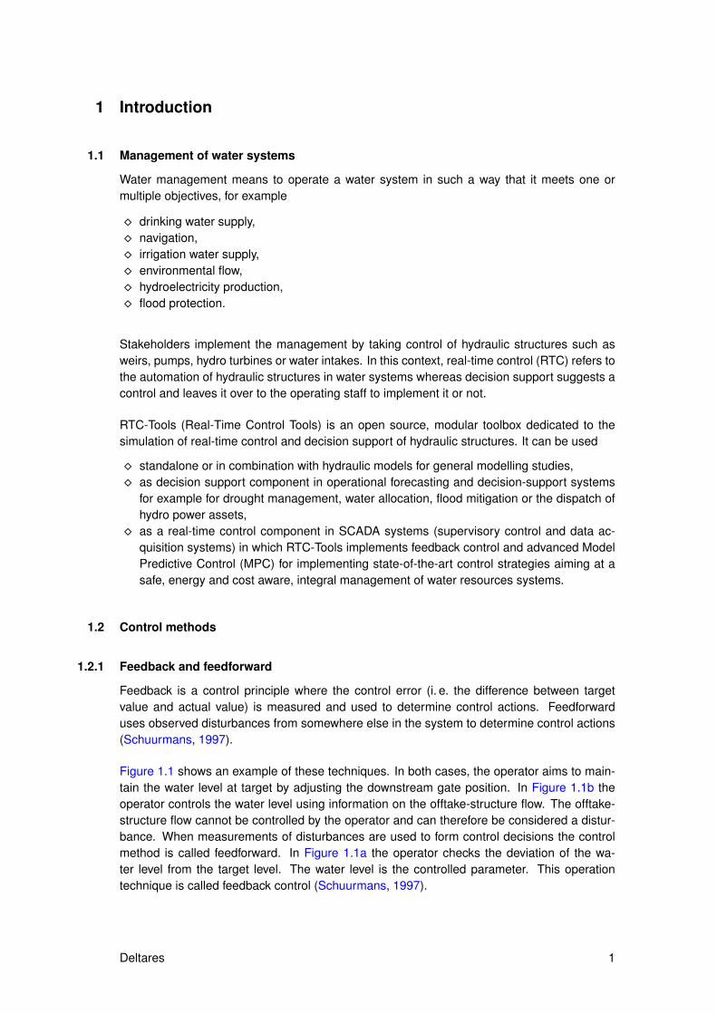
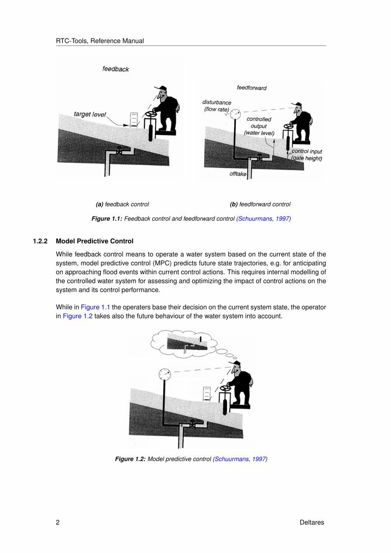
Feedback is a control principle where the control error (i. e. the difference between targetvalue and actual value) is measured and used to determine control actions. Feedforwarduses observed disturbances from somewhere else in the system to determine control actions(Schuurmans, 1997).

Figure 1.1 shows an example of these techniques. In both cases, the operator aims to main-tain the water level at target by adjusting the downstream gate position. In Figure 1.1b theoperator controls the water level using information on the offtake-structure flow. The offtake-structure flow cannot be controlled by the operator and can therefore be considered a distur-bance. When measurements of disturbances are used to form control decisions the controlmethod is called feedforward. In Figure 1.1a the operator checks the deviation of the wa-ter level from the target level. The water level is the controlled parameter. This operationtechnique is called feedback control (Schuurmans, 1997).

Deltares 1


(a) feedback control (b) feedforward control

Figure 1.1: Feedback control and feedforward control (Schuurmans, 1997)

1.2.2 Model Predictive Control

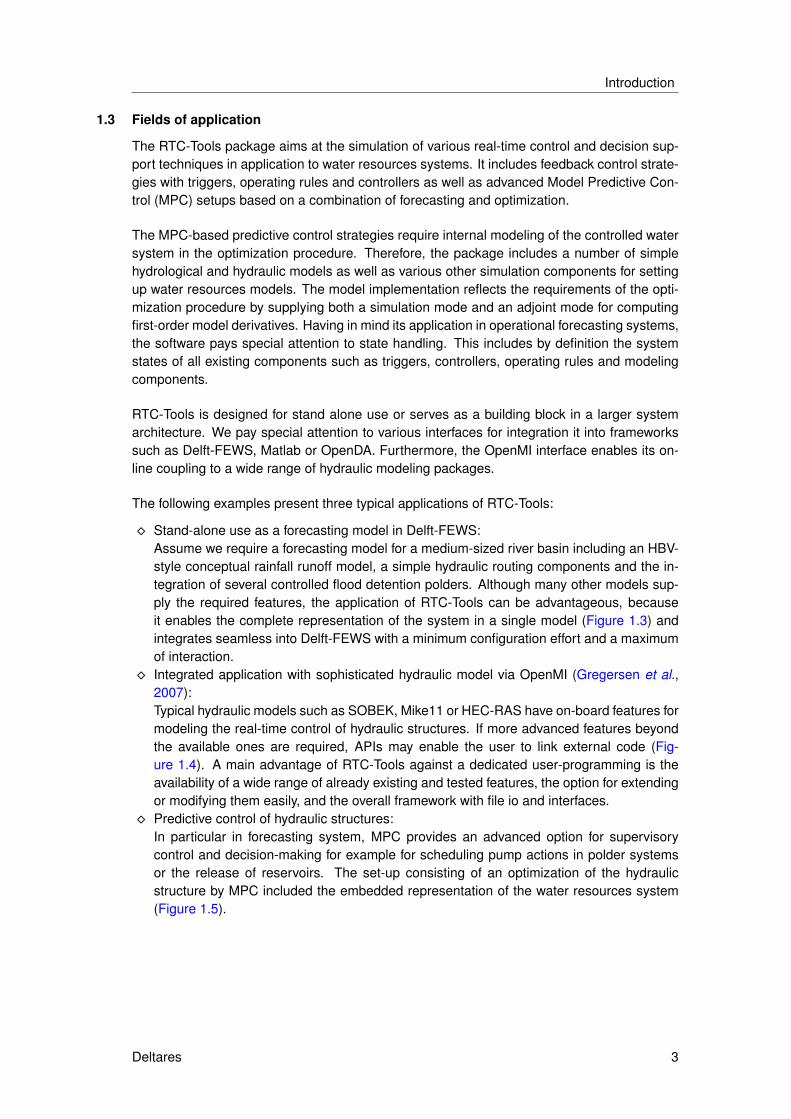
While feedback control means to operate a water system based on the current state of thesystem, model predictive control (MPC) predicts future state trajectories, e.g. for anticipatingon approaching flood events within current control actions. This requires internal modelling ofthe controlled water system for assessing and optimizing the impact of control actions on thesystem and its control performance.

While in Figure 1.1 the operaters base their decision on the current system state, the operatorin Figure 1.2 takes also the future behaviour of the water system into account.

Figure 1.2: Model predictive control (Schuurmans, 1997)

2 Deltares

Introduction

1.3 Fields of application

The RTC-Tools package aims at the simulation of various real-time control and decision sup-port techniques in application to water resources systems. It includes feedback control strate-gies with triggers, operating rules and controllers as well as advanced Model Predictive Con-trol (MPC) setups based on a combination of forecasting and optimization.

The MPC-based predictive control strategies require internal modeling of the controlled watersystem in the optimization procedure. Therefore, the package includes a number of simplehydrological and hydraulic models as well as various other simulation components for settingup water resources models. The model implementation reflects the requirements of the opti-mization procedure by supplying both a simulation mode and an adjoint mode for computingfirst-order model derivatives. Having in mind its application in operational forecasting systems,the software pays special attention to state handling. This includes by definition the systemstates of all existing components such as triggers, controllers, operating rules and modelingcomponents.

RTC-Tools is designed for stand alone use or serves as a building block in a larger systemarchitecture. We pay special attention to various interfaces for integration it into frameworkssuch as Delft-FEWS, Matlab or OpenDA. Furthermore, the OpenMI interface enables its on-line coupling to a wide range of hydraulic modeling packages.

The following examples present three typical applications of RTC-Tools:

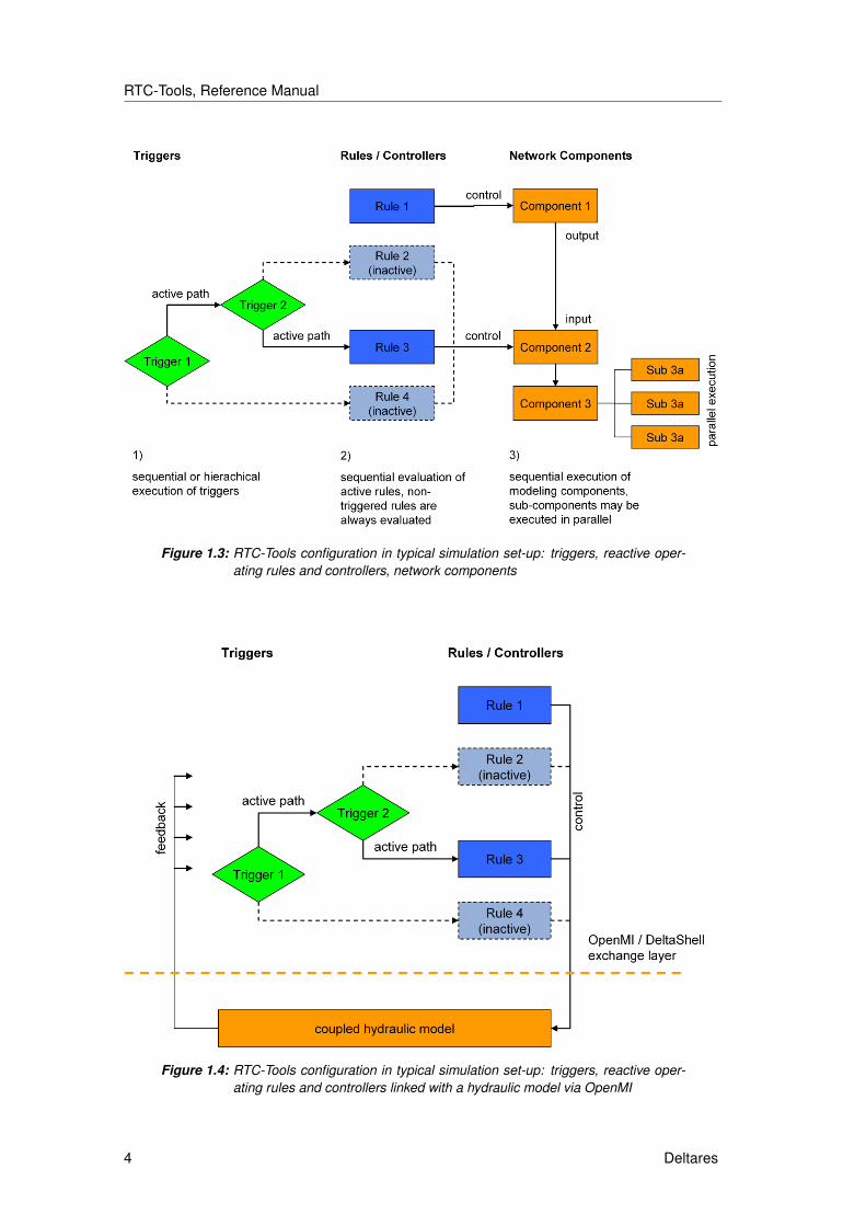
� Stand-alone use as a forecasting model in Delft-FEWS:Assume we require a forecasting model for a medium-sized river basin including an HBV-style conceptual rainfall runoff model, a simple hydraulic routing components and the in-tegration of several controlled flood detention polders. Although many other models sup-ply the required features, the application of RTC-Tools can be advantageous, becauseit enables the complete representation of the system in a single model (Figure 1.3) andintegrates seamless into Delft-FEWS with a minimum configuration effort and a maximumof interaction.

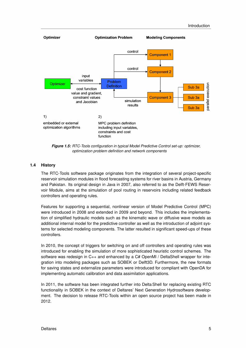
� Integrated application with sophisticated hydraulic model via OpenMI (Gregersen et al.,2007):Typical hydraulic models such as SOBEK, Mike11 or HEC-RAS have on-board features formodeling the real-time control of hydraulic structures. If more advanced features beyondthe available ones are required, APIs may enable the user to link external code (Fig-ure 1.4). A main advantage of RTC-Tools against a dedicated user-programming is theavailability of a wide range of already existing and tested features, the option for extendingor modifying them easily, and the overall framework with file io and interfaces.

� Predictive control of hydraulic structures:In particular in forecasting system, MPC provides an advanced option for supervisorycontrol and decision-making for example for scheduling pump actions in polder systemsor the release of reservoirs. The set-up consisting of an optimization of the hydraulicstructure by MPC included the embedded representation of the water resources system(Figure 1.5).

Deltares 3


Figure 1.3: RTC-Tools configuration in typical simulation set-up: triggers, reactive oper-ating rules and controllers, network components

Figure 1.4: RTC-Tools configuration in typical simulation set-up: triggers, reactive oper-ating rules and controllers linked with a hydraulic model via OpenMI

4 Deltares

Introduction

Figure 1.5: RTC-Tools configuration in typical Model Predictive Control set-up: optimizer,optimization problem definition and network components

1.4 History

The RTC-Tools software package originates from the integration of several project-specificreservoir simulation modules in flood forecasting systems for river basins in Austria, Germanyand Pakistan. Its original design in Java in 2007, also referred to as the Delft-FEWS Reser-voir Module, aims at the simulation of pool routing in reservoirs including related feedbackcontrollers and operating rules.

Features for supporting a sequential, nonlinear version of Model Predictive Control (MPC)were introduced in 2008 and extended in 2009 and beyond. This includes the implementa-tion of simplified hydraulic models such as the kinematic wave or diffusive wave models asadditional internal model for the predictive controller as well as the introduction of adjoint sys-tems for selected modeling components. The latter resulted in significant speed-ups of thesecontrollers.

In 2010, the concept of triggers for switching on and off controllers and operating rules wasintroduced for enabling the simulation of more sophisticated heuristic control schemes. Thesoftware was redesign in C++ and enhanced by a C# OpenMI / DeltaShell wrapper for inte-gration into modeling packages such as SOBEK or Delft3D. Furthermore, the new formatsfor saving states and externalize parameters were introduced for compliant with OpenDA forimplementing automatic calibration and data assimilation applications.

In 2011, the software has been integrated further into Delta Shell for replacing existing RTCfunctionality in SOBEK in the context of Deltares’ Next Generation Hydrosoftware develop-ment. The decision to release RTC-Tools within an open source project has been made in2012.

Deltares 5


OpenDA / DAToolsdata assimilation forachieving optimum

system states

RTC Toolsreal-time control onhydraulic structures

PI-interface

OpenMI interface

Delft-FEWSintegration

any OpenMIcompliant modellingpackage such as:

SOBEKDelft3D

feedback control:- operating rules- controllers- triggers

model predictive control:- nonlinear optimizers- optimization problem

definition

various internal models

this block can be definedin RTC Tools directly orexternally in Matlab

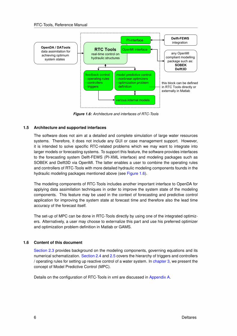
Figure 1.6: Architecture and interfaces of RTC-Tools

1.5 Architecture and supported interfaces

The software does not aim at a detailed and complete simulation of large water resourcessystems. Therefore, it does not include any GUI or case management support. However,it is intended to solve specific RTC-related problems which we may want to integrate intolarger models or forecasting systems. To support this feature, the software provides interfacesto the forecasting system Delft-FEWS (PI-XML interface) and modeling packages such asSOBEK and Delft3D via OpenMI. The latter enables a user to combine the operating rulesand controllers of RTC-Tools with more detailed hydraulic modeling components founds in thehydraulic modeling packages mentioned above (see Figure 1.6).

The modeling components of RTC-Tools includes another important interface to OpenDA forapplying data assimilation techniques in order to improve the system state of the modelingcomponents. This feature may be used in the context of forecasting and predictive controlapplication for improving the system state at forecast time and therefore also the lead timeaccuracy of the forecast itself.

The set-up of MPC can be done in RTC-Tools directly by using one of the integrated optimiz-ers. Alternatively, a user may choose to externalize this part and use his preferred optimizerand optimization problem definition in Matlab or GAMS.

1.6 Content of this document

Section 2.3 provides background on the modeling components, governing equations and itsnumerical schematization. Section 2.4 and 2.5 covers the hierarchy of triggers and controllers/ operating rules for setting up reactive control of a water system. In chapter 3, we present theconcept of Model Predictive Control (MPC).

Details on the configuration of RTC-Tools in xml are discussed in Appendix A.

6 Deltares

2 Simulation components

2.1 Overview

Modelling components in RTC-Tools represent water resources systems and cover the sim-ulation of rainfall runoff and routing based on physically-based, conceptual or data-drivenapproaches. Hydraulic structures in these components can be controlled by (i) operatingrules and controllers in combination with triggers or (ii) by predictive control techniques. Thefirst option is based on simulation as well, so that the triggers, operating rules and controllersbecome part of an overall simulation model. The configuration of RTC-Tools distinguishesthree layers for (1) triggers, (2) operating rules and controllers and (3) modeling components(Table 2.1). This chapter covers all three layers of simulation components (1)–(3) as well asgeneral purpose simulation components such as the lookup table which are used in more thanone layer.

According to our definition, a trigger implements conditions for

� defining when an operating rule, controller or another trigger is applied� returning true or false, e. g. if a threshold is crossed or not.

Operating rules and controllers

� define how a structure operates,� return a value for a control parameter, e.g. a gate opening or turbine release, which is

picked up in one of the modeling components.

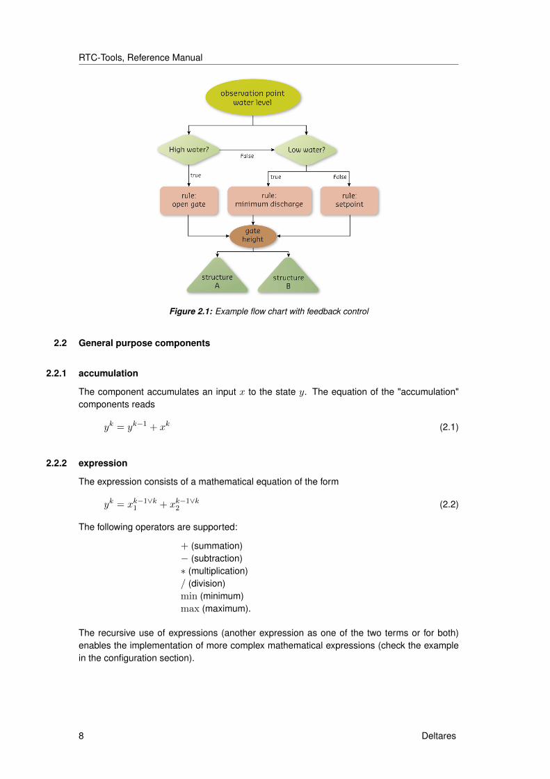
The combination of triggers with operating rules and controllers may form binary decisiontrees such as given in Figure 2.1 for representing hierarchical conditions leading to uniquecontrol actions.

From a mathematical point of view, all features in this chapter compute their outputs fromavailable data either from the previous time step k−1 or from output of previous components ofthe same time step k. Note that triggers always are evaluated first, before rules and modelingcomponents.

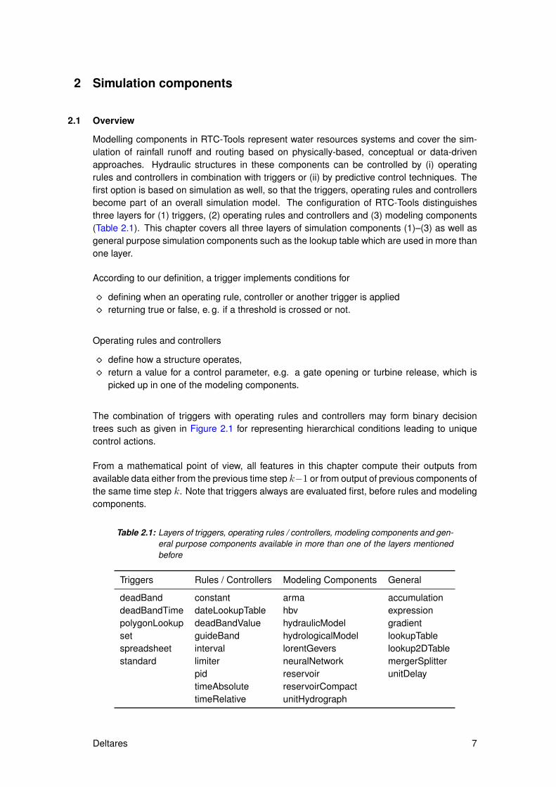
Table 2.1: Layers of triggers, operating rules / controllers, modeling components and gen-eral purpose components available in more than one of the layers mentionedbefore

Triggers Rules / Controllers Modeling Components General

deadBand constant arma accumulationdeadBandTime dateLookupTable hbv expressionpolygonLookup deadBandValue hydraulicModel gradientset guideBand hydrologicalModel lookupTablespreadsheet interval lorentGevers lookup2DTablestandard limiter neuralNetwork mergerSplitter

pid reservoir unitDelaytimeAbsolute reservoirCompacttimeRelative unitHydrograph

Deltares 7


Figure 2.1: Example flow chart with feedback control

2.2 General purpose components

2.2.1 accumulation

The component accumulates an input x to the state y. The equation of the "accumulation"components reads

yk = yk−1 + xk (2.1)

2.2.2 expression

The expression consists of a mathematical equation of the form

yk = xk−1∨k1 + xk−1∨k

2 (2.2)

The following operators are supported:

+ (summation)− (subtraction)∗ (multiplication)/ (division)min (minimum)max (maximum).

The recursive use of expressions (another expression as one of the two terms or for both)enables the implementation of more complex mathematical expressions (check the examplein the configuration section).

8 Deltares

Simulation components

2.2.3 gradient

The governing equation of the gradient reads:

yk =xk − xk−1

∆t(2.3)

2.2.4 lookupTable

The rule supplies a piecewise linear 1D lookup table according to

yk = f(xk−1∨k) (2.4)

This rule is a simpler version of the dateLookupTable (section 2.4.2).

2.2.5 lookup2DTable

The rule supplies a piecewise linear 2D lookup table according to

yk = f(xk−1∨k1 , xk−1∨k

2 ) (2.5)

2.2.6 mergerSplitter

The merger rule provide a simple data hierarchy by choosing the output y equal to the firstof several input values x1, x2, ..., xn which is non-missing. Furthermore, additional outputincludes the sum of all input values.

2.2.7 unitDelay

The unit delay operator is an auxiliary tool for making data from time steps prior to the previoustime step available in the simulation. By using this operator, we can refer to a historicalrelease, for example in an operating rule, without abandoning the restarting features of themodel based on the system state of a single time step. It reads

yk+1 = xk (2.6)

2.3 Modeling components

2.3.1 arma

The arma model (just an ar(1)-model at the moment) reads

ek =

{xksim − xkobscare

k−1if xkobs is available

otherwise

yk = xksim + ek(2.7)

where xobs is an (external) observation, xsim a simulation, e is the difference between obser-vation and simulation, car is the auto regression coefficient.

Deltares 9


2.3.2 hbv

This model is currently under development.

2.3.3 hydraulicModel

2.3.3.1 Introduction

Hydraulic routing, compared to the hydrological routing techniques presented above, is a moreaccurate approach and may include the simulation of hysteresis and backwater effects. Onthe other hand, hydraulic routing has more demands with respect to the numerical solution,computational effort, and may become unstable if not properly implemented and set-up.

RTC-Tools includes a hydraulic routing method based on a mixed kinematic and diffusivewave approach. The most relevant decisions to make are the choice of an appropriate routing(kinematic / diffusive), spatial schematization (central / upwind) and time stepping scheme(explicit / implicit). The following section provides some hints on choosing the proper modeland how to set it up.

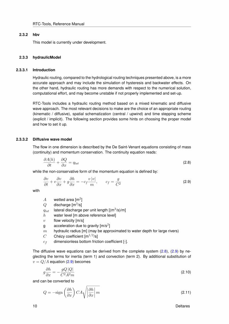
2.3.3.2 Diffusive wave model

The flow in one dimension is described by the De Saint-Venant equations consisting of mass(continuity) and momentum conservation. The continuity equation reads:

∂A(h)

∂t+∂Q

∂x= qlat (2.8)

while the non-conservative form of the momentum equation is defined by:

∂v

∂t+ v

∂v

∂x+ g

∂h

∂x= −cf

v |v|m

, cf =g

C2(2.9)

with

A wetted area [m2]Q discharge [m3/s]qlat lateral discharge per unit length [(m3/s)/m]h water level [m above reference level]v flow velocity [m/s]g acceleration due to gravity [m/s2]m hydraulic radius [m] (may be approximated to water depth for large rivers)C Chézy coefficient [m1/2/s]cf dimensionless bottom friction coefficient [-].

The diffusive wave equations can be derived from the complete system (2.8), (2.9) by ne-glecting the terms for inertia (term 1) and convection (term 2). By additional substitution ofv = Q/A equation (2.9) becomes

g∂h

∂x= − gQ |Q|

C2A2m(2.10)

and can be converted to

Q = −sign

(∂h

∂x

)CA

√∣∣∣∣∂h∂x∣∣∣∣m (2.11)

10 Deltares


s

s

s

sQQ

Q

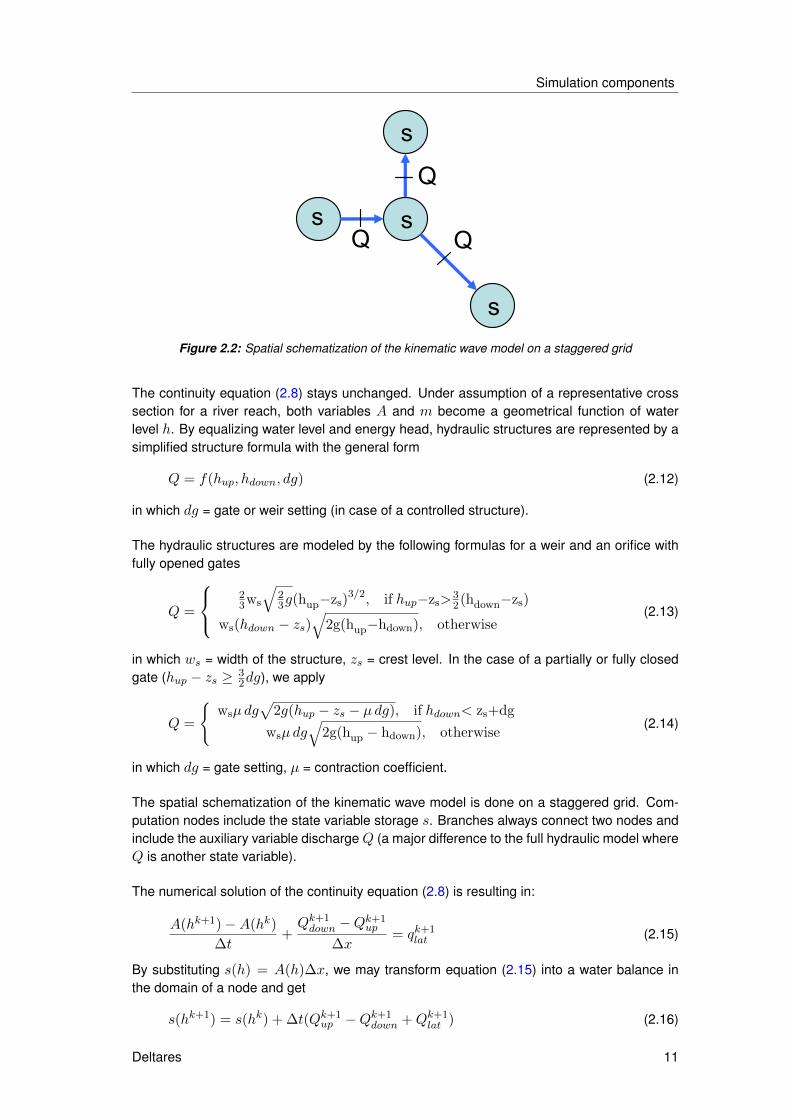
Figure 2.2: Spatial schematization of the kinematic wave model on a staggered grid

The continuity equation (2.8) stays unchanged. Under assumption of a representative crosssection for a river reach, both variables A and m become a geometrical function of waterlevel h. By equalizing water level and energy head, hydraulic structures are represented by asimplified structure formula with the general form

Q = f(hup, hdown, dg) (2.12)

in which dg = gate or weir setting (in case of a controlled structure).

The hydraulic structures are modeled by the following formulas for a weir and an orifice withfully opened gates

Q =

23ws

√23g(hup−zs)

3/2, if hup−zs>32(hdown−zs)

ws(hdown − zs)√

2g(hup−hdown), otherwise(2.13)

in which ws = width of the structure, zs = crest level. In the case of a partially or fully closedgate (hup − zs ≥ 3

2dg), we apply

Q =

{wsµdg

√2g(hup − zs − µdg), if hdown< zs+dg

wsµdg√

2g(hup − hdown), otherwise(2.14)

in which dg = gate setting, µ = contraction coefficient.

The spatial schematization of the kinematic wave model is done on a staggered grid. Com-putation nodes include the state variable storage s. Branches always connect two nodes andinclude the auxiliary variable dischargeQ (a major difference to the full hydraulic model whereQ is another state variable).

The numerical solution of the continuity equation (2.8) is resulting in:

A(hk+1)−A(hk)

∆t+Qk+1down −Q

k+1up

∆x= qk+1

lat (2.15)

By substituting s(h) = A(h)∆x, we may transform equation (2.15) into a water balance inthe domain of a node and get

s(hk+1) = s(hk) + ∆t(Qk+1up −Qk+1

down +Qk+1lat ) (2.16)

Deltares 11


in which s = storage at a node (state variable), Qlat is the total lateral inflow into the domainof the node.

The discharge in a flow branch is schematized based on equation (2.11) by

Qk+1 = f(hkdown, hkup) = −sign

(hkdown − hkup

∆x

)C(hk)A(hk)

√√√√∣∣∣∣∣hkdown − hkup∆x

∣∣∣∣∣m(hk),

(2.17)

in which hk =hkdown+hkup

2

In a branch with a hydraulic structure, the flow branch is replaced by the formula of the hy-draulic structures modeled by an arbitrary equation in the form

Qk+1 = f(hkdown, hkup, dg

k+1) (2.18)

Stability of this method turns out to be reasonable as long as the Courant-Friedrichs-Lewy(CFL) condition is fulfilled.

2.3.3.3 Kinematic versus diffusive wave routing

The fact that the diffusive wave model takes into account more terms of the full dynamicSaint Venant model does not mean that it is always preferred over the simpler kinematic waveapproach. Simplicity and computational performance of the latter may have advantages; inparticular if results of both approaches are the same, e.g. in river reaches with steep gradients.

The following aspects may guide you to the proper approach:

� Is the slope of your river reach smaller than TODO(??): xxx?� Is backwater a relevant effect you need to consider?� Do you want to consider hysteresis?

If you answer one of these questions with “Yes”, consider the diffusive wave approach. Oth-erwise, you may try the kinematic wave method first. Note that you can mix both methods bydefining the related tag in each flow branch.

2.3.3.4 Model set-up

The spatial schematization of your routing network is a trade-off between accuracy (a higherresolution means more accuracy) and CPU time. For flow routing purposes only, already avery course spatial schematization may achieve the required accuracy from the control pointof view. We recommend the following procedure for defining your routing network:

1 Indicate all nodes you need to include: boundary conditions, upstream and downstreamnode of hydraulic structures, stream flow gauges, bifurcations and confluences, nodeswith lateral inflows or extractions (can be also lumped into neighboring nodes).

2 Place additional nodes between the existing ones, if required for accuracy.

All nodes require a level-storage relation. One way to get those is a detailed analysis ofthe surrounding channel network (typically halfway to the next node) in terms of the area

12 Deltares


and storage at different elevations. An easier and often sufficient option is the selection of atypical cross section at the node and its multiplication by the length of the reaches around. Ifyou selected the upwind schematization (see section 3.4.3), take the cross section you areusing in the flow branch.

If you routing network includes flooding and drying, take care that the lowest level of yourlevel-storage table or equation in your node is lower than the lowest elevation in the crosssections around. Since the model implementation does not include any dedicated procedurefor flooding and drying, violating this condition may result in negative water depth at nodesand problems with robustness. If you use the upwind schematization together with the level-storage relation derived from it, this condition is already fulfilled.

Flow branches require a cross section. You may again aim at deriving an aggregated crosssection from the available data of the branch. The simpler approach is again the selection ofa typical cross section. Depending on the spatial schematization (see 3.4.3), select a typicalcross section close to the upstream node for the upwind option and one halfway along thebranch for the central option.

2.3.4 hydrologicalModel


2.3.5 lorentGrevers


2.3.6 neuralNetwork

We use a recurrent neural network formulation given by the following equations for the sum ofneuron µ and the (nonlinear) transfer function

ykµ =

µ−1∑v=1

wneuronµ,v xkv +

K∑v=µ

wneuronµ,v xk−1

v +L∑v=1

winputµ,v ukv

xkµ = hµ

(ykµ

) (2.19)

where

xkν is the value of neuron v at time step k.ykµ is the weighted sum of inputs to neuron µ at time step k.wneuronµ,v is the weighting given to neuron v when calculating the sum for neuron µ.

winputµ,v is the weighting given to input v, when calculating the sum for neuron µ.

ukν is the value of input v at time step k.K is the number of neurons.L is the number of inputs.hµ is the activation function for neuron µ.

Note that the for µ = 1, the first summation term in (2.19) is empty and hence should be takenas zero.

Deltares 13


2.3.7 reservoir

2.3.7.1 Mathematical model

The basic equation for pool routing in a reservoir is

ds

dt= I −Q(h)

h = f(s)(2.20)

where

I inflow into the reservoirQ release of the reservoirs storage in the reservoir (state variable)h water level in the reservoirt time.

We assume the relation f() between storage s and water level h to be a function or a piece-wise linear lookup table.

The release Q from the reservoir can be further subdivided into an into a controlled releaseQc and an uncontrolled release Qu according to

Q(h, dg) = Qc(h, dg) +Qu(h) (2.21)

where dg is the setting of a hydraulic structure. Whereas the controlled release is a functionof the water level h (under assumption that its maximum capacity depends on the water levelin the reservoir) and the setting of the structure dg. The uncontrolled release is only a functionof the reservoir’s water level h representing for example an uncontrolled spillway with a fixedcrest level.

2.3.7.2 Numerical schematization

The explicit schematization, also referred to as "Forward Euler", for the pool routing equationreads

sk = sk−1 + ∆t(Ik −Qkc (hk−1, dgk)−Qku(hk−1)) (2.22)

and is conditionally stable for sufficiently small time steps. The unconditionally stable implicitversion is

sk = sk−1 + ∆t((1− θ)Ik−1 + θIk)

− (1− θ)Qk−1c (hk−1, dgk−1)− θQkc (hk, dgk)

− (1− θ)Qk−1u (hk−1)− θQku(hk))

(2.23)

where 0.5 ≤ θ ≤ 1.0 is the time weighting coefficient of the "Theta" scheme shifting graduallyfrom a more accurate second-order Crank-Nicholson method for θ = 0.5 to a more robust,first-order "Backward Euler" scheme for θ = 1.0.

14 Deltares


2.3.8 reservoirCompact

This is a dedicated component for hydropower reservoirs with gated spillways. Depending onthe availability of a forebay elevation input zfb, the mass balance equation is either used tocompute the new reservoir storage sk or the reservoir’s mass balance residuum rk. In thecase of no forebay elevation input, the new storage is computed by

sk = sk−1 + ∆t(∑n

QkI,n −QkO)

rk = 0

(2.24)

where QI and QO are reservoir inflows and outflow, respectively, and ∆t is the time step. Inthe case of an available forebay elevation, the mass balance is used to compute the massbalance residuum by

rk =sk(zkfb)− sk−1

∆t−∑n

QkI,n +QkO (2.25)

The first mode is primarily used to simulate reservoirs or optimize them in a sequential mode(check details in Chapter 3). The second mode serves to run the reservoir in update mode,in case of having inflow, outflow and forebay elevation available and checking the reservoir’smass balance. Furthermore, it is used in the simulaneous optimization mode.

The forebay elevation zfb directly depends on the storage given by

zkfb = fls(sk) (2.26)

where the level storage relation fls() can be configured as a piecewise linear lookup table ora polynominal function.

The ’reservoirCompact’ component implements several options for computing the tailwaterelevation ztw according to the equations

zktw = ftw(QkO) (2.27)

zktw = a+ bzk−1fb,d + c(QkO)d (2.28)

zktw = zktw,ext + a(Qk −QkO,ext) (2.29)

where ftw() in Equation (2.27) is a piecewise linear table with the relation between the outflowof the reservoir and the tailwater elevation. Note that this formulation is not taking into accountbackwater effects from downstream projects. Equation (2.28) is a tailwater equation whichconsiders the reservoir’s outflow and the forebay elevation zfb,d of a downstream reservoir.It includes the parameters a, b, c and d. Equation (2.29) makes use of an external tailwaterforecast ztw,ext for a given outflow trajectory QO,ext. The simulated tailwater is computed bya linear variation of the provided, external tailwater and the products of a parameter a andthe difference between the simulated and external outflow. Furthermore, the tailwater can beprovided by an external time series or modeling component.

The head h of the turbines is computed by

hk = zkfb − zktw (2.30)

Deltares 15


Environmental obligations may require spill operations. In this case, the spill is either pro-vided as an absolute flow QS,TGT or provided by a spill rate qS,TGT which is computed aspercentage of the total outflow QO according to

QkS,TGT =qkS,TGT

100QkO (2.31)

The turbine flow QT at an aggregated project level is bounded by the requirement of a mini-mum power production and the maximum turbine capacity in term of a maximum power pro-duction or an external maximum turbine flow QTX,ext provided by

QkTM = fPQ(P kM , hk)

QkTX = min(fPQ(P kX , hk), QkTX,ext)

(2.32)

whereQTM andQTX are the minimum and maximum turbine flows, respectively, PM , PX arethe power production bounds and the function fPQ() provides the relations between power,head and the turbine flow. The function fPQ() and its corresponding inverse function fQP ()are derived from information about the turbine efficiency, which is either provided by a lookuptable as a head dependent efficiency (unit: power / discharge) or by a two-dimensional lookuptable as a dependency on head and flow (dimensionless).

The spill target and the turbine flow bounds in combination with an embedded prioritized re-lease policy enables us to split the total outflow into spill and turbine flow. The minimumgeneration requirements in effect for voltage support are the highest priority objective. Addi-tional outflow is allocated for the spill target, then for additional power generation up to themaximum turbine capacity, and finally directed again to the spill. This implicit outflow distribu-tion enables us to keep the total outflow as a single optimization variable without the need foroptimizing spill and turbine flow separately together with constraints for enforcing a releaseprocedure. The related equations for the spill and turbine flow become

QkS =

QkO −QkTX −QkMISC if QkO > QkTX +QkST +QkMISC

QkST if QkTX +QkST > QkO > QkTM +QkSTQkO −QkTM −QkMISC if QkTM +QkST > QkO > QkTM

0 else

(2.33)

QkT =

QkTX if QkO > QkTX +QkST

QkO −QkST −QkMISC if QkTX +QkST > QkO > QkTM +QkSTQkTM if QkTM +QkST > QkO > QkTM

QkO −QkMISC else

(2.34)

Finally, the power generation of a project is computed by

P k = fQP (QkT , hk) (2.35)

The component can handle SI as well as imperial units. The two options are summarized inTable 2.2.

16 Deltares


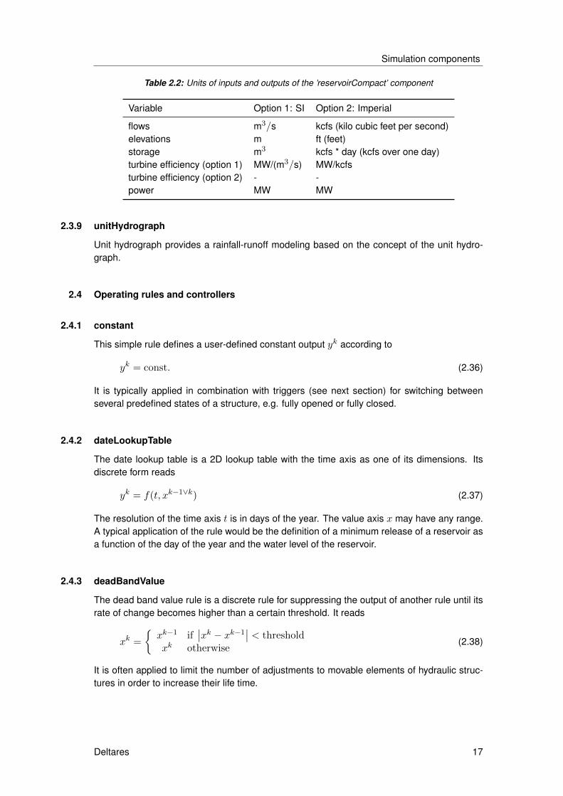
Table 2.2: Units of inputs and outputs of the ’reservoirCompact’ component

Variable Option 1: SI Option 2: Imperial

flows m3/s kcfs (kilo cubic feet per second)elevations m ft (feet)storage m3 kcfs * day (kcfs over one day)turbine efficiency (option 1) MW/(m3/s) MW/kcfsturbine efficiency (option 2) - -power MW MW

2.3.9 unitHydrograph

Unit hydrograph provides a rainfall-runoff modeling based on the concept of the unit hydro-graph.

2.4 Operating rules and controllers

2.4.1 constant

This simple rule defines a user-defined constant output yk according to

yk = const. (2.36)

It is typically applied in combination with triggers (see next section) for switching betweenseveral predefined states of a structure, e.g. fully opened or fully closed.

2.4.2 dateLookupTable

The date lookup table is a 2D lookup table with the time axis as one of its dimensions. Itsdiscrete form reads

yk = f(t, xk−1∨k) (2.37)

The resolution of the time axis t is in days of the year. The value axis x may have any range.A typical application of the rule would be the definition of a minimum release of a reservoir asa function of the day of the year and the water level of the reservoir.

2.4.3 deadBandValue

The dead band value rule is a discrete rule for suppressing the output of another rule until itsrate of change becomes higher than a certain threshold. It reads

xk =

{xk−1 if

∣∣xk − xk−1∣∣ < threshold

xk otherwise(2.38)

It is often applied to limit the number of adjustments to movable elements of hydraulic struc-tures in order to increase their life time.

Deltares 17


xmin xmax

ymin

ymax

Figure 2.3: Graphical representation of guideBand rule

2.4.4 guideBand

The guide band rule provides a linear interpolation from input x to output y, if x is betweentwo input threshold xmin and xmax. Otherwise, the output is limited to defined minimum andmaximum output threshold ymin and ymax. The rule reads

yk =

ymin

ymin + xk−1∨k(ymax−ymin)xmax−xmin

ymax

, ifxk−1∨k ≤ xmin

xmin < xk−1∨k < xmax

xmax ≤ xk−1∨k(2.39)

A graphical representation of the rule is presented in Figure 2.3.

The input and output thresholds xmin, xmax, ymin, ymax can be constant, a function of time orprovided by a time series, e.g. from an external input or a result from the execution of a priorrule.

A typical application of the rule is the enforcement of a reservoir storage s between a cer-tain range and the use of the available storage for equalizing the release. If the storage isapproaching or down-crossing the lower storage limit smin, the release is set to the minimumflow (zero is no minimum flow is defined). If the storage is approaching or up-crossing theupper limit smax, the release is set to maximum capacity.

2.4.5 interval

The interval controller is a simple feedback controller according to the control law

yk =

ymax if xk−1 > spk + 1

2Dymin if xk−1 < spk − 1

2Dyk−1 otherwise

(2.40)

where xk−1 is an input variable, spk is a setpoint, D is a dead band around the setpoint, andyk is the controller output.

18 Deltares


2.4.6 limiter

In contrary to the deadBand rule defined above, the discrete limiter rule restricts the changeof a variable to a relative threshold p. It reads

yk =

(1− p)xk−1

(1 + p)xk−1

xk

if xk < (1− p)xk−1

if xk > (1 + p)xk−1

otherwise(2.41)

where p is the maximum relative rate of change. The configuration also accounts for anabsolute rate of change according to the condition xk < ∆p xk−1 where ∆p is the absoluterate of change.

A typical application of the rule is the limitation of release changes from a reservoir for avoidingtoo steep flow gradients downstream.

2.4.7 pid

The Proportional-Integral-Derivative controller (PID controller) is a generic feedback controllerincluding an optional disturbance term commonly used in industrial control systems. It reads

e(t) = x(t)− sp(t)

y(t) = Kpe(t) +Ki

∫ t

0e(τ)dτ +Kd

d

dte(t) +Kfd(t)

(2.42)

where e(t) is the difference between a process variable x(t) and a setpoint sp(t), Kp,Ki,Kd

are the proportional, integral and derivate gains, respectively, the optional feed forward termconsists of a multiplicator Kf and an external disturbance d(t), y(t) is the controller output.

The discrete form of equation (2.42) in RTC-Tools reads

ek = xk−1 − spk−1

Ek = Ek−1 + ∆t ek

yk = Kpek +KiE

k +Kdek − ek−1

∆t+Kfd

k

(2.43)

where E is the integral of e. The implentation includes a limitation of the maximum velocityaccording to

yk =

(1−∆t∆ymax)yk−1

(1 + ∆t∆ymax)yk−1

yk

if yk < (1−∆t∆ymax)xk−1

if yk > (1 + ∆t∆ymax)xk−1

otherwise(2.44)

Furthermore, the integral part is corrected by a wind-up correction according to

eIk ≤ymax −Kpe

k +KiEk −Kd

ek−ek−1

∆t −Kfdk

Ki

eIk ≥ymin −Kpe

k +KiEk −Kd

ek−ek−1

∆t −Kfdk

Ki

, (2.45)

if the minimum and maximum settings of the actuator are met.

Deltares 19


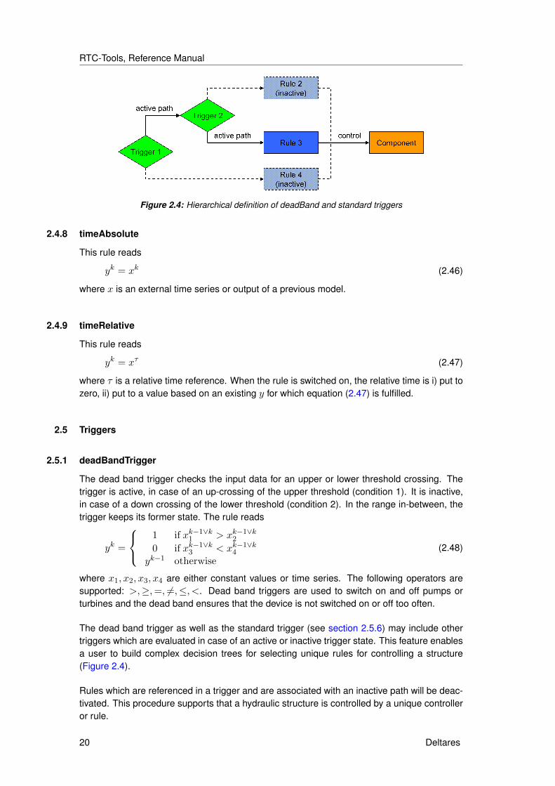
Figure 2.4: Hierarchical definition of deadBand and standard triggers

2.4.8 timeAbsolute

This rule reads

yk = xk (2.46)

where x is an external time series or output of a previous model.

2.4.9 timeRelative

This rule reads

yk = xτ (2.47)

where τ is a relative time reference. When the rule is switched on, the relative time is i) put tozero, ii) put to a value based on an existing y for which equation (2.47) is fulfilled.

2.5 Triggers

2.5.1 deadBandTrigger

The dead band trigger checks the input data for an upper or lower threshold crossing. Thetrigger is active, in case of an up-crossing of the upper threshold (condition 1). It is inactive,in case of a down crossing of the lower threshold (condition 2). In the range in-between, thetrigger keeps its former state. The rule reads

yk =

1 if xk−1∨k

1 > xk−1∨k2

0 if xk−1∨k3 < xk−1∨k

4

yk−1 otherwise

(2.48)

where x1, x2, x3, x4 are either constant values or time series. The following operators aresupported: >,≥,=, 6=,≤, <. Dead band triggers are used to switch on and off pumps orturbines and the dead band ensures that the device is not switched on or off too often.

The dead band trigger as well as the standard trigger (see section 2.5.6) may include othertriggers which are evaluated in case of an active or inactive trigger state. This feature enablesa user to build complex decision trees for selecting unique rules for controlling a structure(Figure 2.4).

Rules which are referenced in a trigger and are associated with an inactive path will be deac-tivated. This procedure supports that a hydraulic structure is controlled by a unique controlleror rule.

20 Deltares


2.5.2 deadBandTime

The dead band time trigger checks a time series for a number of subsequent up-crossingsnup or down-crossing ndown from its current value. If the crossing is observed for at least theuser-defined number of time steps, the new value is used. The trigger reads

xk =

xk if {xk−nup+1, ..., xk} > xk−nup

xk if {xk−ndown+1, ..., xk} < xk−ndown

xk−1 otherwise(2.49)

An application for this trigger is the activation or deactivation of alarm levels. The increaseof alarm level may happen immediately (nup = 0), whereas the decrease of an alarm levelcould be done only after a number of n time steps have passed (ndown = n) without furtherthreshold crossings.

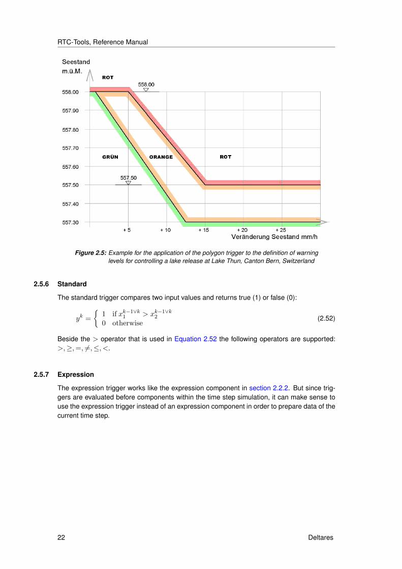
2.5.3 polygonLookup

The polygon lookup trigger checks, if a point is inside of a set of polygons. If this is the case,it returns the user-defined value of the specific polygon. The point is defined by the values oftwo time series, referred to as the x1 and x2 coordinate of the point. The rule reads

yk =

y1...yn

ydefault

if (xk−1∨k1 , xk−1∨k

2 ) ∈ P1...

if (xk−1∨k1 , xk−1∨k

2 ) ∈ Pnotherwise

(2.50)

where y is the result of the rule and {P1, ..., Pn} is a set of polygons.

Figure 2.5 presents an example for the application of the trigger to the definition of warninglevel for controlling a lake release in Canton Bern, Switzerland.

2.5.4 set

The trigger enables a logical combination of other triggers, combined by a logical operator. Itreads

yk = xk−1∨k1 ∧ xk−1∨k

2 (2.51)

The following operators are supported: ∧ (AND), ∨ (OR), XOR.

If more than two terms needs to be combined, the set can be used recursively by defininganother set as one of the two terms. Therefore, the expression yk = xk1 ∧ (xk2 ∨ xk3) isrepresented by a hierarchy of two sets (check the example in the configuration chapter).

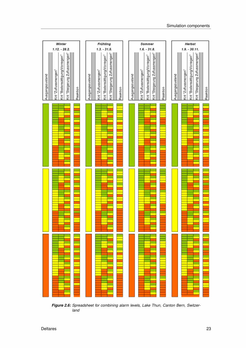
2.5.5 spreadsheet

The spreadsheet trigger enables the definition of a new trigger state based on its old state anda maximum number of three additional inputs. Besides off (0), on (1) states, all other positiveinteger values larger than 1 can be processed.

Figure 2.6 shows an application of the trigger to the combination of alarm levels for Lake Thun,Canton Bern, Switzerland.

Deltares 21


Figure 2.5: Example for the application of the polygon trigger to the definition of warninglevels for controlling a lake release at Lake Thun, Canton Bern, Switzerland

2.5.6 Standard

The standard trigger compares two input values and returns true (1) or false (0):

yk =

{1 if xk−1∨k

1 > xk−1∨k2

0 otherwise(2.52)

Beside the > operator that is used in Equation 2.52 the following operators are supported:>,≥,=, 6=,≤, <.

2.5.7 Expression

The expression trigger works like the expression component in section 2.2.2. But since trig-gers are evaluated before components within the time step simulation, it can make sense touse the expression trigger instead of an expression component in order to prepare data of thecurrent time step.

22 Deltares


Figure 2.6: Spreadsheet for combining alarm levels, Lake Thun, Canton Bern, Switzer-land

Deltares 23


24 Deltares

3 Optimization components

3.1 Introduction and deterministic optimization setup

We consider a discrete time dynamic system according to

xk = f(xk−1, xk, uk, dk)

yk = g(xk, uk, dk)(3.1)

where x, y, u, d are respectively the state, dependent variable, control and disturbance vec-tors, and f(), g() are functions representing an arbitrary linear or nonlinear water resourcesmodel. If being applied in Model Predictive Control (MPC), (3.1) is used for predicting futuretrajectories of the state x and dependent variable y over a finite time horizon represented byk = 1, ..., N time instants, in order to determine the optimal set of controlled variables u byan optimization algorithm. Under the hypothesis of knowing the realization of the disturbanced over the time-horizon, i.e. the trajectory {dk}N1 , a Sequential MPC approach, also referredto as Single Shooting, can be formulated as follows

minu∈{0..T}

N∑k=1

J(xk(u, d), yk, uk) + E(xN (u, d), yN , uN )

subject to h(xk(u, d), yk, uk, dk) ≤ 0, k = 1, ..., N

(3.2)

where xk(u, d), yk are the simulation results, J() is a cost function associated with each statetransition, E() is an additional cost function associated to the final state condition, and h()are hard constraints. In the corresponding simultaneous or collocated optimization approach,the states x become additional variables of the optimization problem, and the process model(3.1), gets an equality constraint of the optimization problem according to

minu,x,y∈{0..T}

N∑k=1

J(xk, yk, uk) + E(xN , yN , uN )

subject to h(xk, yk, uk, dk) ≤ 0, k = 1, ..., N

xk − f(xk−1, xk, uk, dk) = 0

yk − g(xk, uk, dk) = 0

(3.3)

Both methods lead to identical solutions, but have pros and cons for specific optimizationproblems in terms of runtime performance. The sequential approach (3.2) is more efficient,if hard constraints are defined on the control variables u only and gets inefficient for hardconstraints on states x. Because of the state dependency on all prior control variables u, theconstraint Jacobian becomes dense in the lower trianglar matrix. In this case, the simultane-ous approach (3.3) shows better efficiency, since states become an input of the optimizer andthe constraint Jacobian gets sparse.

RTC-Tools does not strictly distinguish between one and the other approach. In fact, opti-mization problems can be set up either in a sequential or simultaneous way. Furthermore,both methods can be mixed leading to the so-called multiple-shooting approach. The choicedepends on the setup of the specific modelling components. For example, the pool routingin a reservoir can be configured in such a way that the control variable is the release only,and the reservoir level is a result of a simulation. Alternatively, the optimizer may provideboth release and reservoir level for computing the mass balance residuum which becomes an

Deltares 25


Table 3.1: Model predictive control features implemented in RTC-Tools

Optimizer MPC problem definition

IPOPT (embedded) constraintsMINOS (Matlab/TOMLAB) min/max bounds and rate of change limitsSNOPT (Matlab/TOMLAB) for optimization variables, system states, outputs

cost function termsrate of change with variable exponentabsolute with variable exponentseveral performance indicators

equality constraint of the optimization problem. It is obvious that the first setup correspondsto the sequential (3.2), the second one to the simultaneous approach (3.3).

3.2 Multi-stage stochastic optimization setup

The extension of the deterministic to a stochastic optimization is achieved by replacing thesingle-trace forecast by a forecast ensemble and computing the objective function valuesJ and E as the probability-weighted sum of the objective function terms of the individualensemble branches or scenarios. This lead to a reformulation of Sequential MPC approachof Equation (3.2) as

minu∈{0..T}

M∑j=1

pj

[N∑k=1

J(xj,k(u), yj,k(x, u), uj,k) + E(xj,N (u), yj,N (x, u), uj,N )

](3.4)

where pj is the probability of the scenario j = 1, . . . ,M and M is the total number of scenar-ios. Whereas the disturbance d as well as the model states x and outputs y are treated inde-pendently in each scenario, the control variable u is the key to the properties of the stochasticoptimization approach. The most general formulation is achieved by the use of scenario trees.One way for its definition is the scenario tree nodal partition matrix P (j, k) with the dimen-sions m× n. The matrix assigns the control at time step k of scenario j to the control vectoru. This enables us to define a common control trajectory for all scenarios at the beginning ofthe forecast horizon when future system states are still uncertain.

When uncertainty gets resolved over the forecast horizon, for example when a forecastedprecipitation is finally observed, we introduce branching points to receive an independentcontrol in each scenario at the end of the forecast horizon. Equation (3.5) presents an exampleof a nodal partition matrix for a simple tree with two scenarios and a branching point at thesecond time step.

P =

[1 2 3 41 2 5 6

](3.5)

The introduction of multiple branching points at several time steps leads to a multi-stagestochastic optimization. From a technical perspective, the solution of the multi-stage stochas-tic optimization (Equation (3.4)) is very similar to the solution of the deterministic setup ofEquation (3.2). The main difference is the number of dimensions of the optimization prob-lem. According to our experience, it is typically increasing by a factor of 5-20, if we derive thescenario tree from a meteorological ensemble forecast.

26 Deltares

Optimization components

The extension of the Simultaneous MPC approach to a multi-stage stochastic optimization isidetical to the one of the sequential approach presented above. An addition is the handling ofhard constraints on system states and outputs. These are executed independently on everybranch of the tree.

3.3 Set-up of the optimization problem

3.3.1 Control variables

The setup of the optimization problem starts with the definition of the input variables of the op-timizer, i.e. the control u in the sequential setup as well as the optional state x and dependentvariable y in the simultaneous setup. Each variable can be of the types

� CONTINUOUS, representing a continuous variable� INTEGER, representing an integer variable (Note that there is still no RTC-Tools-internal

solver supporting Mixed Integer Nonlinear Programming (MINLP), therefore, this optionsdepends on interfacing a suitable solver via the Matlab or GAMS interfaces)

� TIMEINSTANT for the setup of a Time-Instant Optimization MPC (TIO-MPC) (experimentalversion!)

The optimization variable may includes optional bounds for the according to umin ≤ u ≤umax. In case of the TIMEINSTANT of the TIO-MPC, the minimum and maximum boundsare compulsary and represent the two states of the control variable. At each time instant, thestate is switches from one value to the other.

Each optimization variable can include a scaling factor. It is good practice to scale all variablesin such a way that they are in the same order of magnitude. For example, if variables coverboth reservoir levels and releases, the scaling factor of the level should be defined in such asway that its range, i.e. the difference between maximum and minimum operating levels of thereservoirs, multiplied by the scaling factor is in the range of the releases. User-defined scalingusually outperformed automatic, built-in scaling options of the optimizers.

The time step of the control variable u and the simulation can be different. This enablesa courser discretization in the optimization compared to the simulation, for example in caseof using an explicit model with severe time step restrictions. At this moment, the followingaggregation options are supported:

� BLOCK, keeping the the recent value persistent until a new value is specified� LINEAR, conducting a linear interpolation of the control variable between two instants at

which it is defined by the optimization algorithm

Deltares 27


3.3.2 Constraints

RTC-Tools takes into account constraints in two ways: i) as a soft constraint in the objectivefunction or ii) as a hard constraint. This section covers the definition of hard constraint eitheras an inequality constraint or equality constraint of the optimization problem. The next sectionprovides more details on the definition of soft constraints and the objective function in general.

Hard constraints are available for control variables, states or dependent variables. In all cases,the entity may have bounds and a maximum rate of change according to

umin ≤ uk ≤ umax

∆umin ≤ uk − uk−n ≤ ∆umax n = k −N, ..., k − 1(3.6)

where N is the number of time steps of the rate of change constraint looking back in time.

The definition of constraints on control variables is straightforward both in the sequential andsimultaneous optimization setup and requires no additional information. Constraints on statesand dependent variables is only efficient in the simultaneous setup and require informationon how these are traced back to optimization variables. This includes the definition of therelated optimization variables, the modeling components involved and the number of timesteps looking back in time.

Example 1:

Consider a reservoir represented by the mass balance equation below in simultaneous opti-mization mode, represented by

rk = sk − sk−1 −∆t(Qkin −Qkout) (3.7)

where r is the residuum of the mass balance, s and Qout are the two optimization variablesfor reservoir storage and release, respectively. For defining an equality constraint on theresiduum r, we consider a bound constraints with rmin = rmax = 0 and define a stateconstraint referring to the two optimization variables s and Qout, the modeling componentabove and N = 2 time steps (note that the storage at sk−1 and sk contributes to the massbalance equation).

Example 2:

Let’s add a tailwater curve to the reservoir given by

twk = f(Qkout) (3.8)

and define two constraints for i) keeping a minimum tailwater level and ii) limiting the maximumtailwater rate of change

i) twk ≤ twmin

ii) ∆twmin ≤ twk − twk−1 ≤ ∆twmax

(3.9)

The implementation of the first constraint considers the variable Qout, refers to the modelingcomponents (3.8) and requires N = 1. The second constraint works in the same way exceptfor the need for looking back an additional time step in time leading to N = 2.

Note that the Matlab interface provides a platform for defining more general constraints via auser programming.

28 Deltares


3.3.3 Cost function terms

RTC-Tools supports the following cost function terms:

absolute (difference related to a set point)

J = wT∑k=1

∣∣∣uk − usp∣∣∣a (3.10)

where w is a weighting coefficient, usp is a constant or time-dependent set point. The abso-lute term can be applied either on a control, state or dependent variable. The configurationsupports the neglection of the upper branch (u > usp) or lower branch (u < usp) of the valuerange primarily for implementing a soft constraint on a variable up-crossing or down-crossinga threshold.

rate of change (difference of two subsequent values)

J = wT∑k=1

∣∣∣uk − uk−1 − usp∣∣∣a (3.11)

where u is either a control, state or dependent variable, w is a weighting coefficient, and uspis an optional set point for the rate of change. The latter is again primarily used within softconstraints in combination with the neglection of the upper branch (uk−uk−1 > usp) or lowerbranch (uk − uk−1 < usp) of the value range.

Furthermore, additional objective function terms of arbitrary types can be defined in Matlab.

3.4 Adjoint models

Gradient-based solvers of the Sequential Quadratic Programming (SQP) or Interior Point (IP)types require the gradient vector of the cost function dJ(x, u)/du and the constraint Jacobiandh(x, u)/du for performing efficiently. The computation of these first-order derivatives bynumerical differentiation is a straighforward approach, but requires at least n+nnz+1 modelexecution for an optimization problem of n control variables and nnz non-zero entries in theconstraint Jacobian. It becomes computationally inefficient for several hundreds or thousandsof dimensions, and disqualifies the approach from being applied in an operational setting.

A significantly more efficient method for computing the derivatives at computational costs inthe order of a single model execution is the set-up of an adjoint model for each modelingcomponent. The RTC-Tools framework takes care for integrating these models both in thesimulation mode as well as the reverse adjoint mode.

The set-up of an adjoint model is outlined for the explicit version of the diffusive wave modelpresented in section 3.2.1. Consider the mass balance equation given by

sk = sk−1 + ∆t∑i

f(sk−1, sk−1i , dgki ) (3.12)

where s represent the storage at the node of interest and si is the storage at a connected nodei and the function f() denotes the flow contribution of a flow branch or hydraulic structure.

A straightforward way for the derivation of an adjoint model of an explicit calculation workflowis the application of algorithmic differentiation in reverse mode. It is basically a consequent

Deltares 29


application of the chain rule leading to

sk−1 = sk

[1 + ∆t

∑i

∂f(sk−1, sk−1i , dgki )

∂sk−1

]

sk−1i = sk

[1 + ∆t


∂sk−1i

]

dgk

= sk

[∆t


∂dgki

] (3.13)

where u is the adjoint variable of u.

We compute the cost function gradient according to the following procedure:

1 Model simulation, (3.12), for computing all states and dependent variables2 Initialization of the adjoint variables by the partial derivatives of the objective function,uk = ∂J(uk, xk, yk)/∂uk, with respect to control variables, states and dependent vari-ables.

3 Model execution in adjoint mode, (3.13), in reverse order (with respect to the time loopand the execution of subsequent modeling components)

After conducting the steps above, the resulting adjoint variables represent the total derivativesof the cost function dJ(uk, xk, yk)/duk, i.e. the cost function gradient.

The computation of the constraint Jacobian is similar. The following procedure holds for asingle constraint at a specific time step k:

1 ditto (once for all constraints)2 Initialization of the adjoint variables by the partial derivatives of the constraint,uk = ∂h(uk, xk, yk, dk)/∂uk, with respect to control variables, states and dependentvariables.

3 Model execution in adjoint mode, (3.13), over N time steps which contribute to the non-zero Jacobian entries of the specific constraint.

Adjoint systems are still not implemented for all available components in RTC Tool. Anoverview about the status of implementation is given in Table 3.2

30 Deltares


Table 3.2: Implementation status of adjoint models

Adjoint available Comments

Modeling components

accumulation yes -arma yes -expression yes -gradient yes -hydraulicModel yes implementation is only available for the ex-

plicit scheme, implicit scheme will becomeavailable soon

hydrologicalModel no -merger yes -neuralNetwork yes -reservoir yes -reservoirBPA yes -unitDelay yes -unitHydrograph yes -

Rules

all no the adjoint of smooth rules such as the PIDcontroller may become implemeneted in thefuture for modeling mixed systems with MPCand feedback control

Triggers

all no triggers switching on external input will besupported in the future

Deltares 31


32 Deltares

4 References

Becker, B., 2013. Inzet RTC-Tools voor het boezemmodel “Wetterskip Fryslân”. Report1205773-000, Deltares, Delft. In Dutch. 37

Becker, B. P. J., D. Schwanenberg, T. Schruff and M. Hatz, 2012. “Conjunctive real-timecontrol and hydrodynamic modelling in application to Rhine River.” In Proceedings of 10thInternational Conference on Hydroinformatics. TuTech Verlag TuTech Innovation GmbH,Hamburg, Germany. 37

Gregersen, J., P. Gijsbers and S. Westen, 2007. “OpenMI: Open modelling Interface.” Journalof Hydroinformatics 9 (3): 175–191. 3

Schuurmans, J., 1997. Control of Water Levels in Open-Channels. Ph.D. thesis, TechnischeUniversiteit Delft. 1, 2

Schwanenberg, D., B. Becker and T. Schruff, 2011. SOBEK-Grobmodell des staugeregeltenOberrheins. Report no. 1201242-000-ZWS-0014, Deltares. In German. 37

Deltares 33


34 Deltares

A Configuration

A.1 Model setup in XML

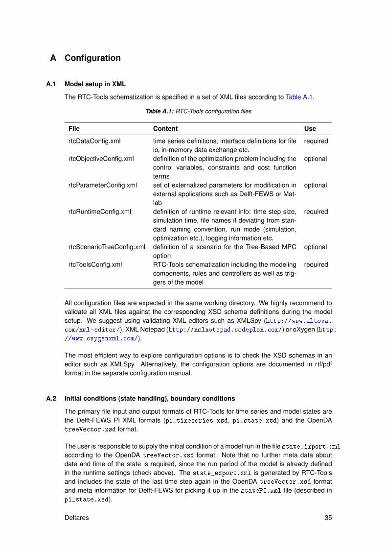
The RTC-Tools schematization is specified in a set of XML files according to Table A.1.

Table A.1: RTC-Tools configuration files

File Content Use

rtcDataConfig.xml time series definitions, interface definitions for fileio, in-memory data exchange etc.

required

rtcObjectiveConfig.xml definition of the optimization problem including thecontrol variables, constraints and cost functionterms

optional

rtcParameterConfig.xml set of externalized parameters for modification inexternal applications such as Delft-FEWS or Mat-lab

optional

rtcRuntimeConfig.xml definition of runtime relevant info: time step size,simulation time, file names if deviating from stan-dard naming convention, run mode (simulation,optimization etc.), logging information etc.

required

rtcScenarioTreeConfig.xml definition of a scenario for the Tree-Based MPCoption

optional

rtcToolsConfig.xml RTC-Tools schematization including the modelingcomponents, rules and controllers as well as trig-gers of the model

required

All configuration files are expected in the same working directory. We highly recommend tovalidate all XML files against the corresponding XSD schema definitions during the modelsetup. We suggest using validating XML editors such as XMLSpy (http://www.altova.com/xml-editor/), XML Notepad (http://xmlnotepad.codeplex.com/) or oXygen (http://www.oxygenxml.com/).

The most efficient way to explore configuration options is to check the XSD schemas in aneditor such as XMLSpy. Alternatively, the configuration options are documented in rtf/pdfformat in the separate configuration manual.

A.2 Initial conditions (state handling), boundary conditions

The primary file input and output formats of RTC-Tools for time series and model states arethe Delft-FEWS PI XML formats (pi_timeseries.xsd, pi_state.xsd) and the OpenDAtreeVector.xsd format.

The user is responsible to supply the initial condition of a model run in the file state_import.xmlaccording to the OpenDA treeVector.xsd format. Note that no further meta data aboutdate and time of the state is required, since the run period of the model is already definedin the runtime settings (check above). The state_export.xml is generated by RTC-Toolsand includes the state of the last time step again in the OpenDA treeVector.xsd formatand meta information for Delft-FEWS for picking it up in the statePI.xml file (described inpi_state.xsd).

Deltares 35

http://www.altova.com/xml-editor/

http://www.altova.com/xml-editor/

http://xmlnotepad.codeplex.com/

http://www.oxygenxml.com/

http://www.oxygenxml.com/


Import and export time series comply with the PI-XML format pi_timeseries.xsd. Bothversion of the format are supported: i) pure XML, ii) a combination of XML and binary files(more efficient, but less readable). The time series of the PI-XML XML file are linked to thetime series in the RTC-Tools (see file rtcDataConfig.xml) by the unique combination oflocationId, parameterId and ensembleIndex.

A.3 Command line options

RTC-Tools expects the XSD schemas in the directory of the binaries. Furthermore, it assumesits working directory in the folder from where it is executed. Both assumption can be overruledby the following command line options:

� -schemaDir=<path to schema directory>

� -workDir=<path to work directory>

A.4 RTC-Tools in Delft-FEWS

We recommend the following setup of the file system for implementing RTC-Tools under Delft-FEWS:

<Delft-FEWS regional home><Modules>

<RTCTools><bin> (including the executables and XSD schemas)rtcDataConfig.xml (configuration of time series and file io)rtcRuntimeConfig.xml (configuration of runtime settings)rtcToolsConfig.xml (configuration of the modeling components)run.bat (batch file for executing a model run)state_import.xml

timeseries_import.xml

Note that the files above represent the minimum set of a RTC-Tools model.

The following hints summaries our recommended "best practice" for implementing RTC-Toolsmodel in Delft-FEWS:

� Use a consistent naming convention between Delft-FEWS and RTC-Tools. We recom-mend to define the RTC-Tools Id by <locationId>_<parameterId>, where the locationand parameter ids are the ones in Delft-FEWS.

� Try to avoid an additional the mapping in Delft-FEWS and use the one in the rtcDataConfig.xml.� Make sure that you use the same units in Delft-FEWS and RTC-Tools. There will be no

unit conversion.� Put the configuration files rtcXXXConfig.xml into a module dataset.� Start with a time series exchange by pure XML, then switch it to the XML/bin option later

for efficiency.

A.5 RTC-Tools in OpenMI

36 Deltares

Configuration

A.5.1 Introduction

For conjunctive modelling of real-time control with hydraulic processes RTC-Tools is equippedwith an interface according to the OpenMI standard. Applications of such conjunctive mod-elling have been described by Becker et al. (2012), Schwanenberg et al. (2011) and Becker(2013). Detailed technical information for an OpenMI composition consisting of RTC-Toolsand SOBEK is given by Schwanenberg et al. (2011) and Becker (2013)

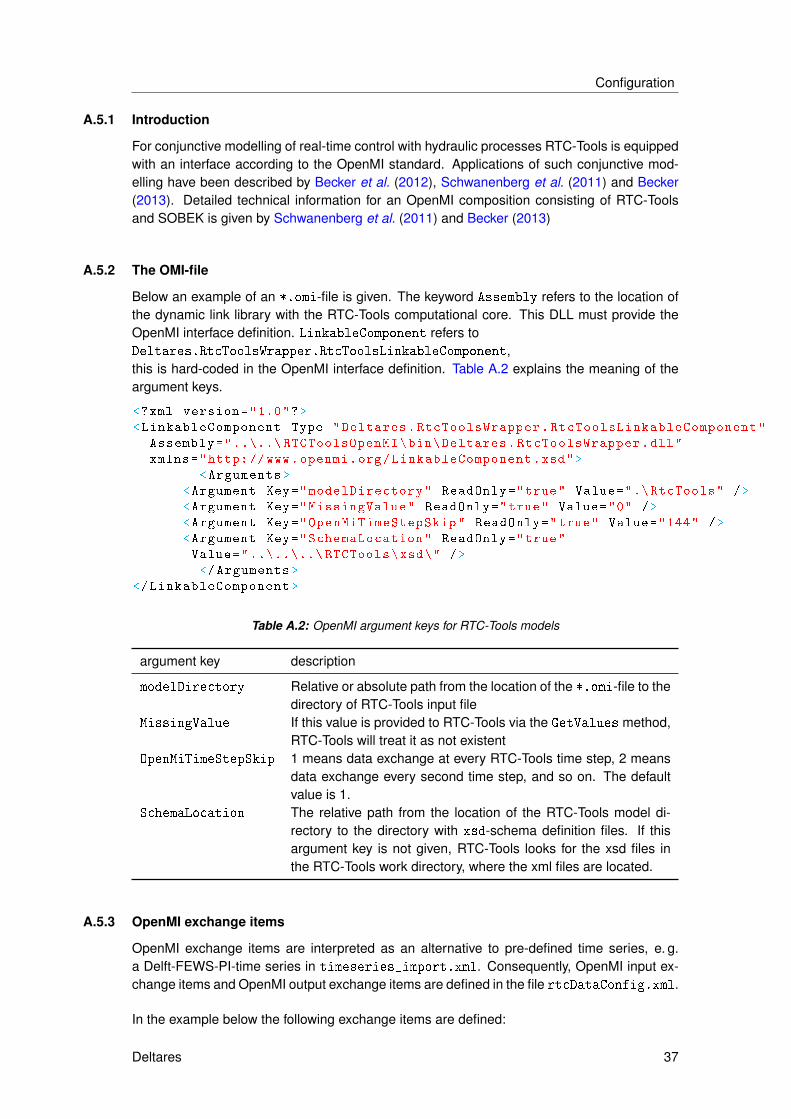
A.5.2 The OMI-file

Below an example of an *.omi-file is given. The keyword Assembly refers to the location ofthe dynamic link library with the RTC-Tools computational core. This DLL must provide theOpenMI interface definition. LinkableComponent refers toDeltares.RtcToolsWrapper.RtcToolsLinkableComponent,this is hard-coded in the OpenMI interface definition. Table A.2 explains the meaning of theargument keys.

<?xml version="1.0"?>

<LinkableComponent Type="Deltares.RtcToolsWrapper.RtcToolsLinkableComponent"

Assembly="..\..\ RTCToolsOpenMI\bin\Deltares.RtcToolsWrapper.dll"

xmlns="http: //www.openmi.org/LinkableComponent.xsd">

<Arguments >

<Argument Key="modelDirectory" ReadOnly="true" Value=".\ RtcTools" />

<Argument Key="MissingValue" ReadOnly="true" Value="0" />

<Argument Key="OpenMiTimeStepSkip" ReadOnly="true" Value="144" />

<Argument Key="SchemaLocation" ReadOnly="true"

Value="..\..\..\ RTCTools\xsd\" />

</Arguments >

</LinkableComponent >

Table A.2: OpenMI argument keys for RTC-Tools models

argument key description

modelDirectory Relative or absolute path from the location of the *.omi-file to thedirectory of RTC-Tools input file

MissingValue If this value is provided to RTC-Tools via the GetValues method,RTC-Tools will treat it as not existent

OpenMiTimeStepSkip 1 means data exchange at every RTC-Tools time step, 2 meansdata exchange every second time step, and so on. The defaultvalue is 1.

SchemaLocation The relative path from the location of the RTC-Tools model di-rectory to the directory with xsd-schema definition files. If thisargument key is not given, RTC-Tools looks for the xsd files inthe RTC-Tools work directory, where the xml files are located.

A.5.3 OpenMI exchange items

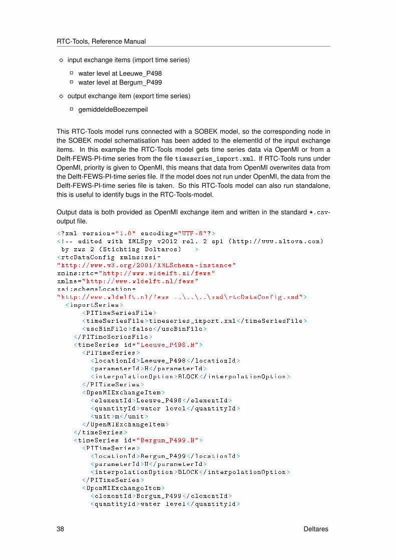
OpenMI exchange items are interpreted as an alternative to pre-defined time series, e. g.a Delft-FEWS-PI-time series in timeseries_import.xml. Consequently, OpenMI input ex-change items and OpenMI output exchange items are defined in the file rtcDataConfig.xml.

In the example below the following exchange items are defined:

Deltares 37

� input exchange items (import time series)

� water level at Leeuwe_P498� water level at Bergum_P499

� output exchange item (export time series)

� gemiddeldeBoezempeil

This RTC-Tools model runs connected with a SOBEK model, so the corresponding node inthe SOBEK model schematisation has been added to the elementId of the input exchangeitems. In this example the RTC-Tools model gets time series data via OpenMI or from aDelft-FEWS-PI-time series from the file timeseries_import.xml. If RTC-Tools runs underOpenMI, priority is given to OpenMI, this means that data from OpenMI overwrites data fromthe Delft-FEWS-PI-time series file. If the model does not run under OpenMI, the data from theDelft-FEWS-PI-time series file is taken. So this RTC-Tools model can also run standalone,this is useful to identify bugs in the RTC-Tools-model.

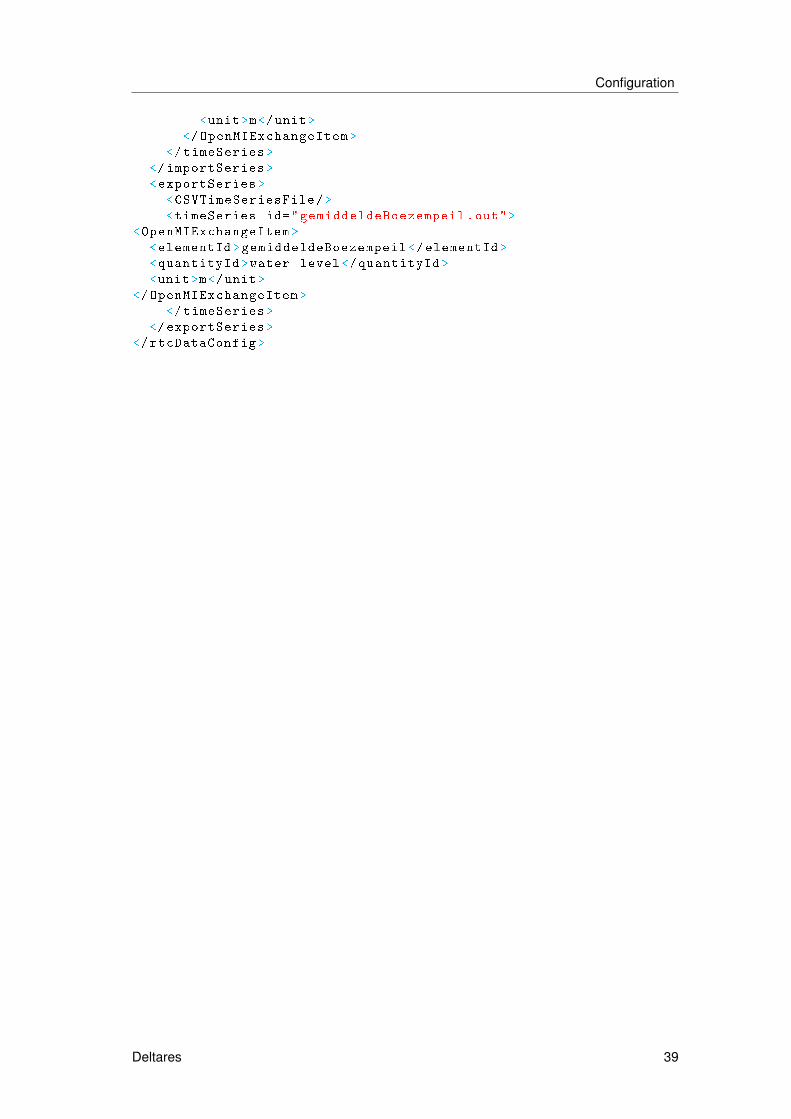
Output data is both provided as OpenMI exchange item and written in the standard *.csv-output file.

<?xml version="1.0" encoding="UTF -8"?>



<rtcDataConfig xmlns:xsi=

"http: //www.w3.org /2001/ XMLSchema -instance"

xmlns:rtc="http: //www.wldelft.nl/fews"

xmlns="http: //www.wldelft.nl/fews"

xsi:schemaLocation=

"http: //www.wldelft.nl/fews ..\..\..\ xsd\rtcDataConfig.xsd">

<importSeries >

<PITimeSeriesFile >

<timeSeriesFile >timeseries_import.xml</timeSeriesFile >

<useBinFile >false</useBinFile >

</PITimeSeriesFile >

<timeSeries id="Leeuwe_P498.H">

<PITimeSeries >

<locationId >Leeuwe_P498 </locationId >

<parameterId >H</parameterId >

<interpolationOption >BLOCK </interpolationOption >

</PITimeSeries >

<OpenMIExchangeItem >

<elementId >Leeuwe_P498 </elementId >

<quantityId >water level</quantityId >

<unit>m</unit>

</OpenMIExchangeItem >

</timeSeries >

<timeSeries id="Bergum_P499.H">

<PITimeSeries >

<locationId >Bergum_P499 </locationId >

<parameterId >H</parameterId >

<interpolationOption >BLOCK </interpolationOption >

</PITimeSeries >


<elementId >Bergum_P499 </elementId >

<quantityId >water level</quantityId >

38 Deltares

Configuration

<unit>m</unit>


</timeSeries >

</importSeries >

<exportSeries >

<CSVTimeSeriesFile/>

<timeSeries id="gemiddeldeBoezempeil.out">


<elementId >gemiddeldeBoezempeil </elementId >

<quantityId >water level </quantityId >

<unit>m</unit>


</timeSeries >

</exportSeries >

</rtcDataConfig >

Deltares 39


40 Deltares

B Errors and unexpected results

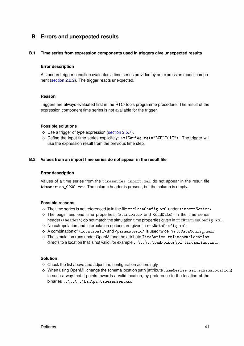
B.1 Time series from expression components used in triggers give unexpected results

Error description

A standard trigger condition evaluates a time series provided by an expression model compo-nent (section 2.2.2). The trigger reacts unexpected.

Reason

Triggers are always evaluated first in the RTC-Tools programme procedure. The result of theexpression component time series is not available for the trigger.

Possible solutions� Use a trigger of type expression (section 2.5.7).� Define the input time series explicitely: <x1Series ref="EXPLICIT">. The trigger will

use the expression result from the previous time step.

B.2 Values from an import time series do not appear in the result file

Error description

Values of a time series from the timeseries_import.xml do not appear in the result filetimeseries_0000.csv. The column header is present, but the column is empty.

Possible reasons� The time series is not referenced to in the file rtcDataConfig.xml under <importSeries>� The begin and end time properties <startDate> and <endDate> in the time series

header (<header>) do not match the simulation time properties given in rtcRuntimeConfig.xml.� No extrapolation and interpolation options are given in rtcDataConfig.xml.� A combination of <locationId> and <parameterId> is used twice in rtcDataConfig.xml.� The simulation runs under OpenMI and the attribute TimeSeries xsi:schemaLocation

directs to a location that is not valid, for example ..\..\..\badFolder\pi_timeseries.xsd.

Solution� Check the list above and adjust the configuration accordingly.� When using OpenMI, change the schema location path (attribute TimeSeries xsi:schemaLocation)

in such a way that it points towards a valid location, by preference to the location of thebinaries ..\..\..\bin\pi_timeseries.xsd.

Deltares 41


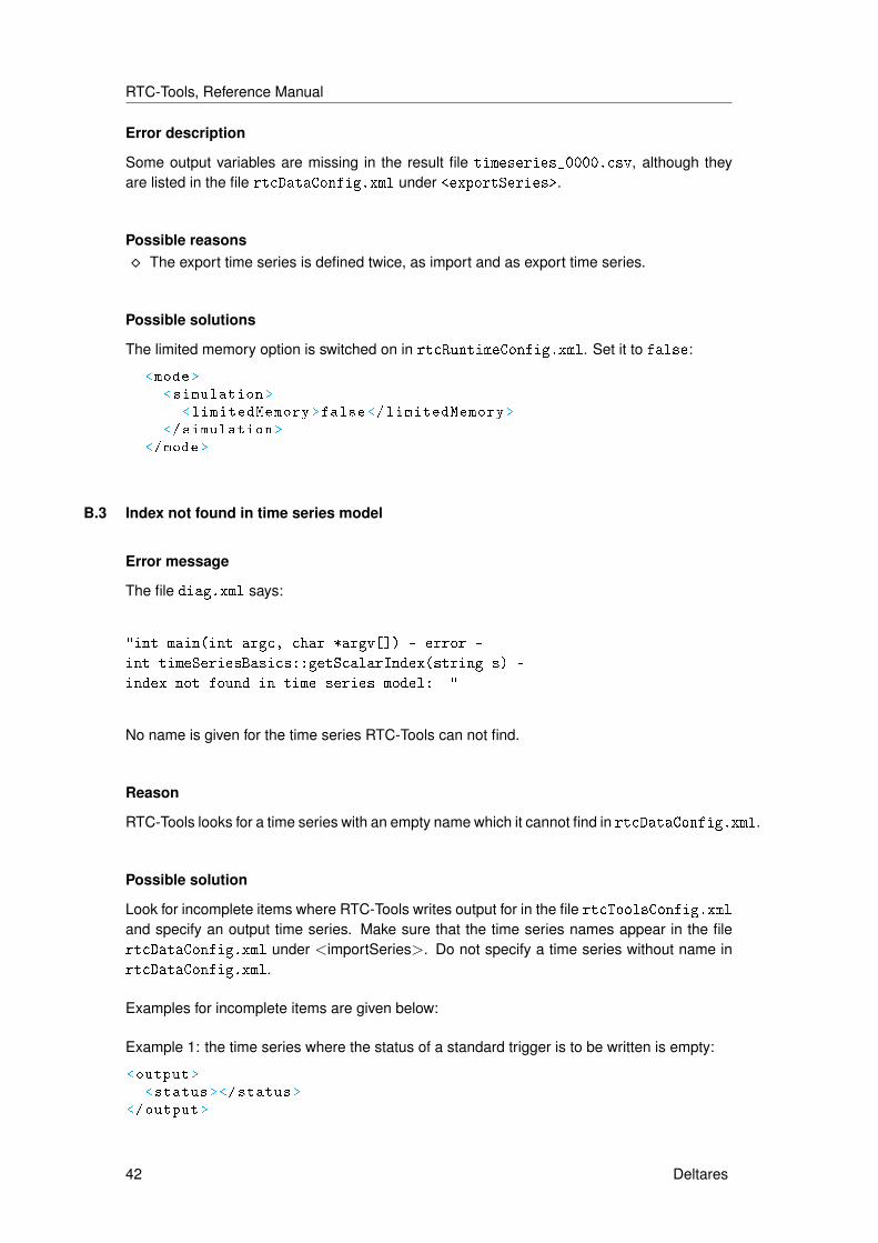
Error description

Some output variables are missing in the result file timeseries_0000.csv, although theyare listed in the file rtcDataConfig.xml under <exportSeries>.

Possible reasons� The export time series is defined twice, as import and as export time series.

Possible solutions

The limited memory option is switched on in rtcRuntimeConfig.xml. Set it to false:

<mode>

<simulation >

<limitedMemory >false </limitedMemory >

</simulation >

</mode>

B.3 Index not found in time series model

Error message

The file diag.xml says:

"int main(int argc, char *argv[]) - error -

int timeSeriesBasics::getScalarIndex(string s) -

index not found in time series model: "

No name is given for the time series RTC-Tools can not find.

Reason

RTC-Tools looks for a time series with an empty name which it cannot find in rtcDataConfig.xml.

Possible solution

Look for incomplete items where RTC-Tools writes output for in the file rtcToolsConfig.xml

and specify an output time series. Make sure that the time series names appear in the filertcDataConfig.xml under <importSeries>. Do not specify a time series without name inrtcDataConfig.xml.

Examples for incomplete items are given below:

Example 1: the time series where the status of a standard trigger is to be written is empty:

<output >

<status ></status >

</output >

42 Deltares

Errors and unexpected results

Example 2: the target time series of an expression is not specified:

<y></y>

Example 3: an input time series is not specified:

<x1Series ref="IMPLICIT"/>

B.4 Instance document parsing failed

Error message

The file diag.xml says:

error - instance document parsing failed"

level="1"

Reason

A file is missing.

Possible solution

Check if all files are available. Most likely the file state_import.xml is missing.

Deltares 43


44 Deltares

C Programming in RTC-Tools (draft version)

C.1 Preface

Contributions to RTC-Tools are welcome. The source code is available in an Apache Sub-version repository (SVN repository) https://svn.oss.deltares.nl/repos/rtc-tools/.We recommend to use a subversion client, for example Tortoise SVN, to checkout the sourcecode from the repository. To request read/write access contact the RTC-Tools product man-agement1. We use Microsoft Visual Studio to compile RTC-Tools code. Microsoft VisualStudio projects are provided within the source code package.

We ask developers for the following:

� To make sure that the new feature fit fits well into the RTC-Tools architecture, we encour-age developers to contact the principal developer2 or RTC-Tools product management todiscuss the ideas.

� Prepare a small test model that illustrates the new feature and add it to the examples inthe svn-repository.

� RTC-Tools is provided in a dual license model:

� as open source under the GNU public license version 2 (GPL2)� under a proprietary license.

The dual license model is necessary to be able to provide features like commercial solversor built-in interfaces to commercial software, which is conflictual to GPL2. Developers musttransfer their intellectual property rights for the added code to Deltares, Deltares in returnguarantees to provide RTC-Tools under GPL2 license.

C.2 Implementing a new feature to RTC-Tools

Below the main working steps to implement new features to RTC-Tools are given.

� Modify the XML schema definition (XSD) file *.xsd. If you want to add a new hydrologicalmodel component newModel in rtcToolsConfig.xml, go to rtcToolsConfig.xsd.

� Define the elements and attributes you need. In most cases they will be of Complex-Type or SimpleType.

� Specify the minimum and maximum number of occurrences (minOccurs, maxOccurs),where minOccurs = 0 means optional.

� Maintain alphabetical order.� Add the newly defined elements to a feasible place in the main tree. Our hydrological

model newModel should be added to the components group.� Validate the xsd file.

� Run the script update_XSD.bat. This script translates the XSD into C++ class files.� Open the source code and go to the files that have been changed by the script update_XSD.bat.� Create a .h-file newModel.h for the new class declaration. Add the variables that are

needed to the class declaration.� The class variables need to be fed with values from the file, in our case rtcToolsConfig.xml.

� Open the schematization.cpp.

[email protected] Schwanenberg ([email protected])

Deltares 45

https://svn.oss.deltares.nl/repos/rtc-tools/


� Add the file newModel.h to the list of include files. Maintain alphabetical order.� Add code to read the data and assign it to the variables

� Create a file newModel.cpp and add the logic of the new feature.

46 Deltares

real time control tools user manual - deltares · typical hydraulic models such as sobek, mike11 or...

Documents