real-time detection of malicious network activity using...
TRANSCRIPT

Real-Time Detection of Malicious Network Activity Using
Stochastic Models
by
Jaeyeon JungSubmitted to the Department of Electrical Engineering and Computer
Sciencein partial fulfillment of the requirements for the degree of
Doctor of Philosophy in Computer Science and Engineering
at the
MASSACHUSETTS INSTITUTE OF TECHNOLOGY
June 2006
c©Massachusetts Institute of Technology 2006. All rights reserved.
Author . . . . . . . . . . . . . . . . . . . . . . . . . . . . . . . . . . . . . . . . . . . . . . . . . . . . . . . . . . . . .Department of Electrical Engineering and Computer Science
May 22, 2006
Certified by . . . . . . . . . . . . . . . . . . . . . . . . . . . . . . . . . . . . . . . . . . . . . . . . . . . . . . . . .Hari Balakrishnan
Professor of Computer Science and EngineeringThesis Supervisor
Accepted by. . . . . . . . . . . . . . . . . . . . . . . . . . . . . . . . . . . . . . . . . . . . . . . . . . . . . . . . .Arthur C. Smith
Chairman, Department Committee on Graduate Students


To my princess Leia

5
Real-Time Detection of Malicious Network Activity Using Stochastic Modelsby
Jaeyeon Jung
Submitted to the Department of Electrical Engineering and Computer Scienceon May 22, 2006, in partial fulfillment of the
requirements for the degree ofDoctor of Philosophy in Computer Science and Engineering
Abstract
This dissertation develops approaches to rapidly detect malicious network traffic includingpackets sent by portscanners and network worms. The main hypothesis is that stochasticmodels capturing a host’s particular connection-level behavior provide a good foundationfor identifying malicious network activity in real-time. Using the models, the dissertationshows that a detection problem can be formulated as one of observing a particular “trajec-tory” of arriving packets and inferring from it the most likely classification for the givenhost’s behavior. This stochastic approach enables us not only to estimate an algorithm’sperformance based on the measurable statistics of a host’s traffic but also to balance thegoals of promptness and accuracy in detecting malicious network activity.
This dissertation presents three detection algorithms based on Wald’s mathematicalframework of sequential analysis. First, Threshold Random Walk (TRW) rapidly detects re-mote hosts performing a portscan to a target network. TRW is motivated by the empiricallyobserved disparity between the frequency with which connections to newly visited localaddresses are successful for benign hosts vs. for portscanners. Second, it presents a hybridapproach that accurately detects scanning worm infections quickly after the infected localhost begins to engage in worm propagation. Finally, it presents a targeting worm detec-tion algorithm, Rate-Based Sequential Hypothesis Testing (RBS), that promptly identifieshigh-fan-out behavior by hosts (e.g., targeting worms) based on the rate at which the hostsinitiate connections to new destinations. RBS is built on an empirically-driven probabilitymodel that captures benign network characteristics. It then presents RBS+TRW, a unifiedframework for detecting fast-propagating worms independently of their target discoverystrategy.
All these schemes have been implemented and evaluated using real packet traces col-lected from multiple network vantage points.
Thesis Supervisor: Hari BalakrishnanTitle: Professor of Computer Science and Engineering


7
Acknowledgments
I am indebted to Hari Balakrishnan for giving me invaluable advice on countless occasionsnot only on research but also on various issues of life. Hari is living evidence that even aman of genius can be warm, kind and always encouraging.
The summer of 2003 at the ICSI Center for Internet Research (ICIR) was one of themost productive periods in my six years of Ph.D study. I am deeply grateful to Vern Paxsonfor his brilliant insights on data analysis, thoughtful discussions, and detailed comments onmy dissertation. I would also like to thank Frans Kaashoek and Robert Morris for theiradvice on the dissertation.
This dissertation would not have been possible without many collaborative efforts withArthur Berger, Rodolfo Milito, Vern Paxson, Stuart Schechter, and Hari Balakrishhan.They demonstrated hard work, clear thinking, and remarkable writing skills that I learnedthrough collaboration with them. I am also grateful to Emre Koksal for answering mytedious questions on stochastic processes.
Kilnam Chon, my advisor at the Korea Advanced Institute of Science and Technology(KAIST) taught me never to be afraid of a challenge and always to tackle a hard problem.During my internship at the Cooperative Association of Internet Data Analysis (CAIDA),K Claffy showed an incredible passion for research. Evi Nemeth was always enthusiasticabout teaching and caring for students. I would like to thank all of them for being greatmentors.
It has been a pleasure to get to know and to work with so many wonderful colleaguesat the Networks and Mobile Systems (NMS) group. Thanks to Magdalena Balazinskafor her sense of humor and friendship; Michel Goraczko for his help on any computerand program related problems; Nick Feamster for collaboration and numerous discussions;Dave Andersen for his encyclopedic knowledge and sharing cute random Web pages; AllenMiu and Godfrey Tan for fun lunch chats. There are also many people on the G9 thathelped me go through many long days. Thanks to Athicha Muthitacharoen, Jinyang Li,Emil Sit, Michael Walfish, and Mythili Vutukuru. Special thanks to Sheila Marian for hertremendous help in dealing with administrative work, for throwing NMS parties and forsqueezing me into always-overbooked Hari’s schedule.
I have been delighted to have many Korean friends at MIT. In particular, I would liketo thank some of them who came to my defense talk to show their support: Youngsu Lee,Alice Oh, Daihyun Lim, and Jaewook Lee. I am eternally grateful to Yunsung Kim forbeing my best friend in high school, in college and at MIT.
I cannot thank my parents, Joonghee Jung and Hanjae Lee, enough for their endlesslove, support, and encouragement. I am a proud daughter of such awesome parents andhope that my daughter, Leia, will feel the same way when she grows up. I would alsolike to thank my brother Jaewoong and parents-in-law, Judy & Lowell Schechter for theirsupport. Finally, I am especially grateful to my husband, Stuart, who is also my scubabuddy, crew mate, and research collaborator.


Contents
1 Introduction 151.1 Malicious Network Activity . . . . . . . . . . . . . . . . . . . . . . . . . 161.2 Challenges to Real-Time Detection . . . . . . . . . . . . . . . . . . . . . . 171.3 Detection Schemes . . . . . . . . . . . . . . . . . . . . . . . . . . . . . . 201.4 Contributions . . . . . . . . . . . . . . . . . . . . . . . . . . . . . . . . . 21
2 Background 252.1 Hypothesis Testing . . . . . . . . . . . . . . . . . . . . . . . . . . . . . . 252.2 Sequential Hypothesis Testing . . . . . . . . . . . . . . . . . . . . . . . . 26
3 Related Work 293.1 Portscan . . . . . . . . . . . . . . . . . . . . . . . . . . . . . . . . . . . . 293.2 Network Virus and Worm Propagation . . . . . . . . . . . . . . . . . . . . 32
4 Portscan Detection 394.1 Data Analysis . . . . . . . . . . . . . . . . . . . . . . . . . . . . . . . . . 414.2 Threshold Random Walk: An Online Detection Algorithm . . . . . . . . . 474.3 Evaluation . . . . . . . . . . . . . . . . . . . . . . . . . . . . . . . . . . . 544.4 Discussion . . . . . . . . . . . . . . . . . . . . . . . . . . . . . . . . . . . 604.5 Summary . . . . . . . . . . . . . . . . . . . . . . . . . . . . . . . . . . . 62
5 Detection of Scanning Worm Infections 655.1 Reverse Sequential Hypothesis Testing . . . . . . . . . . . . . . . . . . . . 685.2 Credit-Based Connection Rate Limiting . . . . . . . . . . . . . . . . . . . 755.3 Experimental Setup . . . . . . . . . . . . . . . . . . . . . . . . . . . . . . 775.4 Results . . . . . . . . . . . . . . . . . . . . . . . . . . . . . . . . . . . . . 795.5 Limitations . . . . . . . . . . . . . . . . . . . . . . . . . . . . . . . . . . 825.6 Summary . . . . . . . . . . . . . . . . . . . . . . . . . . . . . . . . . . . 83
6 Detection of Targeting Worm Propagations 856.1 Data Analysis . . . . . . . . . . . . . . . . . . . . . . . . . . . . . . . . . 876.2 Rate-Based Sequential Hypothesis Testing . . . . . . . . . . . . . . . . . . 916.3 Evaluation . . . . . . . . . . . . . . . . . . . . . . . . . . . . . . . . . . . 956.4 RBS + TRW: A Combined Approach . . . . . . . . . . . . . . . . . . . . 976.5 Discussion . . . . . . . . . . . . . . . . . . . . . . . . . . . . . . . . . . . 105
9

10 CONTENTS
6.6 Summary . . . . . . . . . . . . . . . . . . . . . . . . . . . . . . . . . . . 105
7 Conclusion and Future Directions 107
A Implementation of TRW in Bro policy 111
List of Figures
1-1 The nmap report for tennis.lcs.mit.edu . . . . . . . . . . . . . . . 161-2 Snort rule 103 for the SubSeven trojan horse . . . . . . . . . . . . . . . . . 20
2-1 Sequential Likelihood Ratio Test . . . . . . . . . . . . . . . . . . . . . . . 27
3-1 Virus and worm propagation . . . . . . . . . . . . . . . . . . . . . . . . . 33
4-1 Network intrusion detection system . . . . . . . . . . . . . . . . . . . . . 394-2 CDF of the number of inactive local servers accessed by each remote host . 434-3 CDF of the percentage of inactive local servers accessed by a remote host . 454-4 CDF of the number of distinct IP addresses accessed per remote host . . . . 464-5 Detections based on fixed-size windows: F represents a failure event and S
a success event. . . . . . . . . . . . . . . . . . . . . . . . . . . . . . . . . 484-6 Achieved performance as a function of a target performance . . . . . . . . 514-7 Simulation results . . . . . . . . . . . . . . . . . . . . . . . . . . . . . . . 634-8 Detection speed vs. other parameters . . . . . . . . . . . . . . . . . . . . . 64
5-1 Worm detection system . . . . . . . . . . . . . . . . . . . . . . . . . . . . 665-2 Λ(Y) as each observation arrives . . . . . . . . . . . . . . . . . . . . . . . 695-3 Λ(Y) including events before and after the host was infected . . . . . . . . 705-4 Reverse sequential hypothesis testing . . . . . . . . . . . . . . . . . . . . . 705-5 First-contact connection requests and their responses . . . . . . . . . . . . 715-6 The structure of entries in the First-Contact Connection (FCC) queue . . . . 74
6-1 Worm propagation inside a site . . . . . . . . . . . . . . . . . . . . . . . . 866-2 Fan-out distribution of an internal host’s outbound network traffic . . . . . 896-3 Distribution of first-contact interarrival time . . . . . . . . . . . . . . . . . 906-4 An exponential fit along with the empirical distribution . . . . . . . . . . . 906-5 TH1
and TH0vs. an event sequence . . . . . . . . . . . . . . . . . . . . . . 93
6-6 ln(x) < x− 1 when 0 < x < 1 . . . . . . . . . . . . . . . . . . . . . . . . 956-7 CDF of fan-out rates of non-scanner hosts using a window size of 15, 10, 7
and 5 (from left to right). . . . . . . . . . . . . . . . . . . . . . . . . . . . 976-8 Classification of hosts present in the evaluation datasets . . . . . . . . . . . 1006-9 Simulation results of RBS + TRW for the LBL-II dataset . . . . . . . . . 1036-10 Simulation results of RBS + TRW for the ISP dataset . . . . . . . . . . . . 104
11


List of Tables
1.1 Vulnerabilities listed in the US-CERT database as of July 26, 2005 . . . . . 17
2.1 Four possible outcomes of a decision-making process . . . . . . . . . . . . 26
3.1 Notable computer viruses and worms . . . . . . . . . . . . . . . . . . . . . 37
4.1 Summary of datasets . . . . . . . . . . . . . . . . . . . . . . . . . . . . . 414.2 Remote host characteristics . . . . . . . . . . . . . . . . . . . . . . . . . . 474.3 Simulation results . . . . . . . . . . . . . . . . . . . . . . . . . . . . . . . 564.4 Break-down of “suspects” flagged as H1 . . . . . . . . . . . . . . . . . 584.5 Performance in terms of efficiency and effectiveness . . . . . . . . . . . . . 584.6 Comparison of the number of H1 across three categories for LBL dataset . 594.7 Comparison of the number of H1 across three categories for ICSI dataset . 594.8 Comparison of the efficiency and effectiveness across TRW, Bro, and Snort 60
5.1 Credit-based connection rate limiting . . . . . . . . . . . . . . . . . . . . . 765.2 Summary of network traces . . . . . . . . . . . . . . . . . . . . . . . . . . 785.3 Alarms reported by scan detection algorithm . . . . . . . . . . . . . . . . . 795.4 Alarms reported by virus throttling [76] . . . . . . . . . . . . . . . . . . . 805.5 Composite results for both traces . . . . . . . . . . . . . . . . . . . . . . . 815.6 Comparison of rate limiting by CBCRL vs. virus throttling . . . . . . . . . 815.7 Permitted first-contact connections until detection . . . . . . . . . . . . . . 82
6.1 LBL dataset summary . . . . . . . . . . . . . . . . . . . . . . . . . . . . . 886.2 Scanners detected from the LBL dataset . . . . . . . . . . . . . . . . . . . 896.3 Trace-driven simulation results of RBS varying λ1 . . . . . . . . . . . . . . 966.4 Evaluation datasets: scanning hosts include vulnerability scanners, worm
infectees and hosts that we use proxies for targeting worms because of theiranomalous high-fan-out rate. . . . . . . . . . . . . . . . . . . . . . . . . . 101
6.5 Evaluation of RBS + TRW vs. RBS and TRW . . . . . . . . . . . . . . . . 102
13

Chapter 1
Introduction
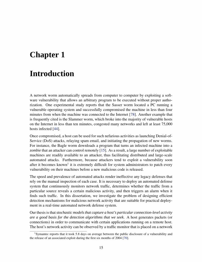
A network worm automatically spreads from computer to computer by exploiting a soft-ware vulnerability that allows an arbitrary program to be executed without proper autho-rization. One experimental study reports that the Sasser worm located a PC running avulnerable operating system and successfully compromised the machine in less than fourminutes from when the machine was connected to the Internet [78]. Another example thatis frequently cited is the Slammer worm, which broke into the majority of vulnerable hostson the Internet in less than ten minutes, congested many networks and left at least 75,000hosts infected [44].
Once compromised, a host can be used for such nefarious activities as launching Denial-of-Service (DoS) attacks, relaying spam email, and initiating the propagation of new worms.For instance, the Bagle worm downloads a program that turns an infected machine into azombie that an attacker can control remotely [15]. As a result, a large number of exploitablemachines are readily available to an attacker, thus facilitating distributed and large-scaleautomated attacks. Furthermore, because attackers tend to exploit a vulnerability soonafter it becomes known1 it is extremely difficult for system administrators to patch everyvulnerability on their machines before a new malicious code is released.
The speed and prevalence of automated attacks render ineffective any legacy defenses thatrely on the manual inspection of each case. It is necessary to deploy an automated defensesystem that continuously monitors network traffic, determines whether the traffic from aparticular source reveals a certain malicious activity, and then triggers an alarm when itfinds such traffic. In this dissertation, we investigate the problem of designing efficientdetection mechanisms for malicious network activity that are suitable for practical deploy-ment in a real-time automated network defense system.
Our thesis is that stochastic models that capture a host’s particular connection-level activityare a good basis for the detection algorithms that we seek. A host generates packets (orconnections) in order to communicate with certain applications running on a remote host.The host’s network activity can be observed by a traffic monitor that is placed on a network
1Symantec reports that it took 5.8 days on average between the public disclosure of a vulnerability andthe release of an associated exploit during the first six months of 2004 [70].
15

16 Chapter 1. Introduction
pathway where those packets pass by. Using such a monitor, we can characterize the host’spatterns of network access based on the metrics such as a connection initiating rate and aconnection failure ratio. In principle, these patterns reflect a host’s activity (i.e., benign Webbrowsing vs. scanning), and we construct models of what constitutes malicious (or benign)traffic and develop online detection problems that promptly identify malicious networkactivity with high accuracy.
The rest of this chapter gives an overview of various malicious network activities intendedto break into a host or to disrupt the service of a variety of network systems; examines thechallenges to detecting such attacks in real-time; reviews previous detection schemes; anddiscusses some of the key contributions of this dissertation.
1.1 Malicious Network Activity
Many Internet attacks involve various network activities that enable remote attackers tolocate a vulnerable server, to gain unauthorized access to a target host, or to disrupt theservice of a target system. In this section, we survey three common malicious activities:vulnerability scanning, host break-in attack, and DoS attack. These three malicious activ-ities are only a subset of many Internet attacks occurring lately, but their prevalence hasdrawn much attention from the research community.
1.1.1 Vulnerability Scanning
There are many tools that allow network administrators to scan a range of the IP addressspace in order to find active hosts and to profile the programs running on each host toidentify vulnerabilities [2,3,4]. These scanning tools, when used by an attacker, can revealsecurity holes at a site that can then be exploited by subsequent intrusion attacks. One suchtool is “nmap”: Figure 1-1 shows that nmap correctly identifies two open ports and theoperating system that tennis.lcs.mit.edu is running.
Starting nmap 3.70 ( http://www.insecure.org/nmap/ )Interesting ports on tennis.lcs.mit.edu (18.31.0.86):PORT STATE SERVICE22/tcp open ssh80/tcp open httpDevice type: general purposeRunning: Linux 2.4.X|2.5.X
Figure 1-1: The nmap report for tennis.lcs.mit.edu
1.1.2 Host Break-in Attack
When a target machine is located, an attacker attempts to break in to the system in order togain unauthorized use of or access to it. The most common method of intrusion is to exploit
1.1. Malicious Network Activity 17
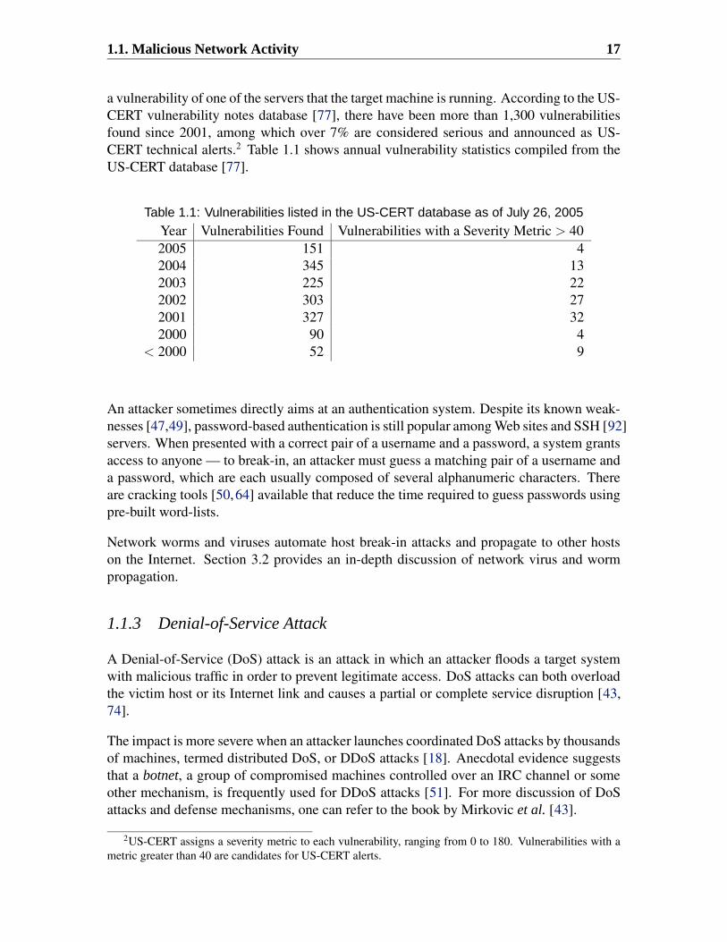
a vulnerability of one of the servers that the target machine is running. According to the US-CERT vulnerability notes database [77], there have been more than 1,300 vulnerabilitiesfound since 2001, among which over 7% are considered serious and announced as US-CERT technical alerts.2 Table 1.1 shows annual vulnerability statistics compiled from theUS-CERT database [77].
Table 1.1: Vulnerabilities listed in the US-CERT database as of July 26, 2005Year Vulnerabilities Found Vulnerabilities with a Severity Metric > 402005 151 42004 345 132003 225 222002 303 272001 327 322000 90 4
< 2000 52 9
An attacker sometimes directly aims at an authentication system. Despite its known weak-nesses [47,49], password-based authentication is still popular among Web sites and SSH [92]servers. When presented with a correct pair of a username and a password, a system grantsaccess to anyone — to break-in, an attacker must guess a matching pair of a username anda password, which are each usually composed of several alphanumeric characters. Thereare cracking tools [50,64] available that reduce the time required to guess passwords usingpre-built word-lists.
Network worms and viruses automate host break-in attacks and propagate to other hostson the Internet. Section 3.2 provides an in-depth discussion of network virus and wormpropagation.
1.1.3 Denial-of-Service Attack
A Denial-of-Service (DoS) attack is an attack in which an attacker floods a target systemwith malicious traffic in order to prevent legitimate access. DoS attacks can both overloadthe victim host or its Internet link and causes a partial or complete service disruption [43,74].
The impact is more severe when an attacker launches coordinated DoS attacks by thousandsof machines, termed distributed DoS, or DDoS attacks [18]. Anecdotal evidence suggeststhat a botnet, a group of compromised machines controlled over an IRC channel or someother mechanism, is frequently used for DDoS attacks [51]. For more discussion of DoSattacks and defense mechanisms, one can refer to the book by Mirkovic et al. [43].
2US-CERT assigns a severity metric to each vulnerability, ranging from 0 to 180. Vulnerabilities with ametric greater than 40 are candidates for US-CERT alerts.

18 Chapter 1. Introduction
1.2 Challenges to Real-Time Detection
To cope with the increasing threat of various Internet attacks, many networks employ sen-sors that monitor traffic and detect suspicious network activity that precedes or accompa-nies an attack. For a network of hundreds (or thousands) of machines, having such sensorsis indispensable because it is a daunting task to ensure that every machine is safe fromknown vulnerabilities, especially when machines are running different operating systemsor network applications.
In this section, we discuss the technical challenges in developing practical and deployablealgorithms that detect malicious network activity in real-time. Each challenge sets up agoal that we intend to meet when designing a detection algorithm. We briefly describe ourgeneral approach to meeting each goal, leaving the detailed discussions for the remainingchapters.
1.2.1 Detection Speed and Accuracy
Many Internet attacks are composed of multiple instances of malicious payload transmis-sions. For instance, scanning activity generates a sequence of probe packets to a set ofdestinations, and a host infected by a computer worm or virus spreads an exploit to manyother vulnerable hosts. Typically, gathering more data improves accuracy as individualpieces of evidence collectively give greater confidence in deciding a host’s intent. A hostthat attempted to access only one non-existent host may have done so because of miscon-figuration rather than scanning activity. In contrast, a host that continued to send packetsto dozens of different non-existent hosts may well be engaged in scanning activity. Animportant question that we aim to answer in this dissertation is the following: how muchdata is enough to determine a host’s behavior with a high level of confidence?
Fast detection is one of the most important requirements of a real-time detection systemalong with high accuracy. The early detection of a port scanner gives network adminis-trators a better chance to block the scanner before it launches an attack: if a scanner hasprobed 25 distinct machines and found 1 vulnerable host that it can exploit, then it maysend out an attack payload immediately. If a scan detection algorithm had been basedon the connection count with a threshold of 20, it could have blocked this attack, but ifthe algorithm had a threshold of 30, it could not have. In principle, as more observationsare needed to make a decision, more malicious traffic will be allowed to pass through thesystem.
The trade-off between accuracy and detection speed complicates the design of a real-timedetection algorithm, and we seek to provide a quantitative framework that allows us togauge an algorithm’s performance. To this end, we design detection algorithms using thesequential hypothesis testing technique [80], which provides a mathematical model forreducing the number of required observations while meeting the desired accuracy criteria.Chapters 4, 5, and 6 present the algorithms developed based on this framework and showthat those detection algorithms significantly speed up the decision process.

1.2. Challenges to Real-Time Detection 19
1.2.2 Evasion
Attackers can craft packets and adjust their behavior in order to evade a detection algorithmonce the algorithm is known. This never-ending arms race between attackers and defensesystems requires that a detection algorithm be resilient to evasion to the possible extent.One way to achieve a high resiliency is to define strict rules for permissible activity suchthat only well-defined network traffic goes through the system. Even so, an attacker mayfind a way to alter its traffic pattern to appear benign. But, such modification often comesat the cost of a significant drop in attack efficiency.
In any case, it is important to precisely define a model for malice and take into considerationpossible variants and exceptional cases that the model may not cover. One possibility is tobuild a stronger defense system by layering multiple independent detection algorithms.For each algorithm that we develop, we discuss the algorithm’s limitations in detail anddescribe what should supplement the algorithm in order to raise the bar.
1.2.3 False Alarms
There are three main reasons for false alarms. First, the model of malicious activity basedon which a detection algorithm operates may include uncommon benign activities. Becauseof the high variation in traffic patterns generated by each application, it is difficult to factorin all the possible cases leading to a false alarm. Hence, it is important to test a detectionalgorithm over real network trace data that include different types of traffic, and to refinethe model such that it eliminates identified false alarms.
Second, the same activity can be regarded as permissible or prohibited depending on a site’ssecurity policy. For example, many peer-to-peer client applications scan other neighboringhosts to find the best peer from which to download a file. This scanning activity can exhibita similar traffic pattern to that of a local host engaged in scanning worm propagation.Depending on a site’s policy on allowing peer-to-peer traffic, flagging a peer-to-peer clientas a scanner can be a legitimate detection or a false alarm. We consider this policy issuein evaluating the performance of our detection algorithm, separating obvious false alarmsfrom policy-dependent ones.
Third, an attacker can spoof an originating IP address so that a detection system erroneouslyflags an otherwise innocent host. This framing attack can cause a “crying wolf” problem:a real attack would not be taken seriously should an immediate response take place. Whileour detection algorithm operates based on the assumption that each source IP address isgenuine, a simple additional component can prevent framing attacks (see Sections 4.4 and5.5 for details).
1.2.4 Scaling Issues
The amount of network traffic determines the amount of input data that a detection systemneeds to analyze in real-time. A detection system employed at a busy network faces thechallenge of processing data at high rates. First, the high volume of input data requires ahigh degree of accuracy. If a detector is designed such that its false alarm rate is 0.001,
20 Chapter 1. Introduction
the actual number of false alarms is that rate multiplied by the number of events generatedby input traffic, which increases proportionally with the amount of traffic arriving at thenetwork monitor.
Second, many operational issues need to be addressed for running a real-time detectionsystem in high-volume networks. As discussed by Dreger et al. [19], factors that impactthe system’s CPU load and memory usage include the type of analysis (e.g., transport-layeranalysis vs. application-layer analysis), the rate of packet arrivals to the detection system,and the amount of connection state to be maintained in memory. Hence, it is crucial tohave efficient resource management schemes in place in order to keep the detection systemoperational as traffic volume rises.
Third, real-time detection algorithms must be efficient enough to not overload the systemwhen the state it maintains grows with respect to traffic. Moreover, an attacker can alsotarget the detection system itself if he knows how to slow it down by consuming too manyresources [52, 54]. The detection system should be aware of how fast the state can growwith respect to the traffic volume and should provide guards that limit its resource usage.
1.3 Detection Schemes
There is a large body of literature that presents, evaluates, and surveys detection approachesof network intrusion attacks. These approaches differ depending on their goal of detectionand set of rules required for operation, but, we can roughly categorize them based on theunderlying detection principle. In this section, we discuss three major detection principleswith emphasis on their strength and weakness.
1.3.1 Misuse Detection
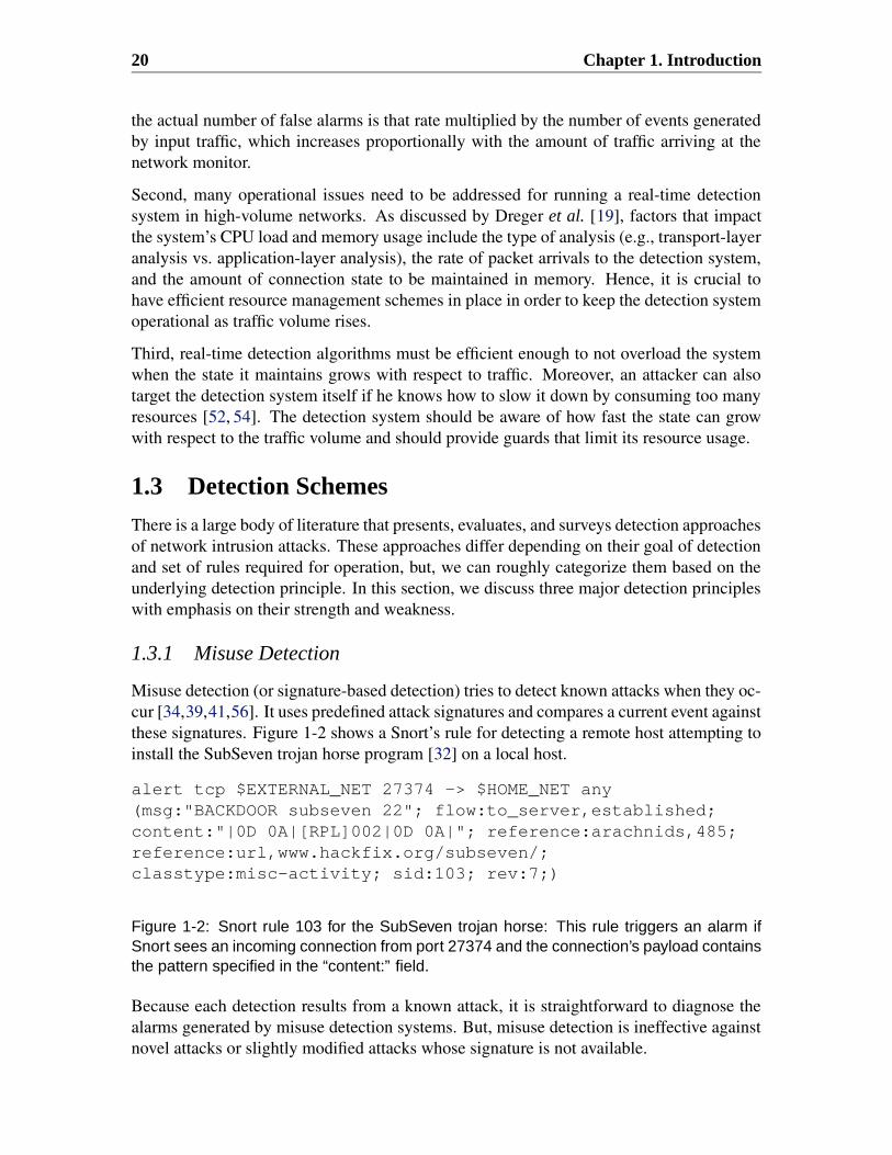
Misuse detection (or signature-based detection) tries to detect known attacks when they oc-cur [34,39,41,56]. It uses predefined attack signatures and compares a current event againstthese signatures. Figure 1-2 shows a Snort’s rule for detecting a remote host attempting toinstall the SubSeven trojan horse program [32] on a local host.
alert tcp $EXTERNAL_NET 27374 -> $HOME_NET any(msg:"BACKDOOR subseven 22"; flow:to_server,established;content:"|0D 0A|[RPL]002|0D 0A|"; reference:arachnids,485;reference:url,www.hackfix.org/subseven/;classtype:misc-activity; sid:103; rev:7;)
Figure 1-2: Snort rule 103 for the SubSeven trojan horse: This rule triggers an alarm ifSnort sees an incoming connection from port 27374 and the connection’s payload containsthe pattern specified in the “content:” field.
Because each detection results from a known attack, it is straightforward to diagnose thealarms generated by misuse detection systems. But, misuse detection is ineffective againstnovel attacks or slightly modified attacks whose signature is not available.

1.4. Contributions 21
1.3.2 Anomaly Detection
Anomaly detection is designed to identify a source exhibiting a behavior deviating fromthat normally observed in a system [7, 31, 42]. The construction of such a detector beginswith developing a model for “normal behavior”. A detection system can learn the normalbehavior by training data sets collected over a certain time period with no intrusions. Itcan also use for detection a set of rules describing acceptable behavior that an operatormanually programmed in.
Anomaly detection is capable of detecting previously unknown attacks so long as thoseattacks form a poor match against a norm. But, it often suffers from a high degree of falsealarms generated by legitimate but previously unseen behavior.
1.3.3 Specification-based Detection
Specification-based detection watches for a source that violates the pre-built program spec-ifications [38, 58]. In particular, programs that run with a high privilege (e.g., SUID rootprograms [30]) need a careful watch since an attacker often targets such programs in orderto execute an arbitrary code.
Like anomaly detection, specification-based detection can detect novel attacks, but the de-velopment of detailed specifications requires thorough understanding of many security-critical programs in a system, which can be a time-consuming process.
1.4 Contributions
This dissertation explores the conjecture that many Internet attacks entail network behaviorthat manifests quite differently from that of a legitimate host. Accordingly, we hypothesizethat stochastic models that capture a host’s network behavior provide a good foundation foridentifying malicious network activity in real-time.
The overall structure of the dissertation is as follows:
• We investigate three malicious network activities: portscan, scanning worm infec-tion, and targeting worm propagation. For each case, we examine real network tracedata that contain both large samples of benign traffic and some instances of malicioustraffic of interest if available.
• We develop detection algorithms based on the mathematical framework of sequentialanalysis founded by Wald in his seminal work [80]. Using a connection between thereal-time detection of malicious network activity and a theory of sequential analysis(or sequential hypothesis testing), we show that one can often model a host’s networkactivity as one of two stochastic processes, corresponding respectively to the accesspatterns of benign hosts and malicious ones.The detection problem then becomes one of observing a particular trajectory andinferring from it the most likely classification for the given host’s behavior. This

22 Chapter 1. Introduction
approach enables us to estimate an algorithm’s performance based on the measurablestatistics of a host’s traffic. More importantly, it provides an analytic framework, withwhich one can balance the goals of promptness and accuracy in detecting maliciousnetwork activity.
• We evaluate each algorithm’s performance in terms of accuracy and detection speedusing network trace data collected from multiple vantage points. While our algo-rithms require only connection-level information (source and destination IP address-es/ports, timestamp, and connection status), we assess the correctness of flaggedcases using various methods such as payload inspection, hostname, and site-specificinformation.
Our contributions in this dissertation are:
1. Portscan Detection: We present an algorithm that rapidly detects remote hosts per-forming a portscan to a target network. Our algorithm, Threshold Random Walk(TRW), is motivated by the empirically observed disparity between the frequencywith which connections to newly visited local addresses are successful for benignhosts vs. for portscanners. To our knowledge, TRW is the first algorithm that pro-vides a quantitative framework explaining the detection speed and the accuracy ofport scan detection. Using trace-driven simulations, we show that TRW is more ac-curate and requires a much smaller number of events (4 or 5 in practice) to detectmalicious activity compared to previous schemes. We published TRW and the per-formance results in [36].
2. Detection of Scanning Worm Infections: We present a hybrid approach that accu-rately detects scanning worm infection promptly after the infected local host beginsto engage in worm propagation. Our approach integrates significant improvementsthat we have made to two existing techniques: sequential hypothesis testing andconnection rate limiting. We show that these two extensions are vital for the fastcontainment of scanning worms:
• Reverse Sequential Hypothesis Testing: To address a problem when an ob-served host can change its behavior, from benign to malicious, we evaluate thelikelihood ratio of a given host being malicious in reverse chronological orderof the observations. We prove that the reverse sequential hypothesis testing isequivalent to the forward sequential hypothesis testing with modifications inthe likelihood ratio computation. This modified forward sequential hypothesistest significantly simplifies algorithmic implementation. Moreover, it has beenshown to be optimal for change point detection [48].• Credit-based Rate Limiting: To ensure that worms cannot propagate rapidly
between the moment scanning begins and the time at which a sufficient num-ber of connection failures has been observed by the detector, we develop anadaptive scheme that limits the rate at which a host issues new connections thatare indicative of scanning activity. Our trace-driven simulation results show

1.4. Contributions 23
that the credit-based rate limiting causes much fewer unnecessary rate limitingsthan the previous scheme, which relies on a fixed 1 new connection per secondthreshold.
We published the scanning worm detection approach and the results in [57].
3. Detection of Targeting Worm Propagations: We present an algorithm that promptlydetects local hosts engaged in targeting worm propagation. Our algorithm, Rate-Based Sequential Hypothesis Testing (RBS), is built on the rate at which a hostinitiates a connection to a new destination. RBS promptly detects hosts that ex-hibit abnormal levels of fan-out rate, which distinguishes them from benign hostsas they are working through a list of potential victims. Derived from the theory ofsequential hypothesis testing, RBS dynamically adapts its window size and thresh-old, based on which it computes a rate and updates its decision in real-time. Wethen present RBS+TRW, a unified framework for detecting fast-propagating wormsindependently of their target discovery strategy. This work is under submission.
Like misuse detection and specification-based detection, we need to build a priori models,but, unlike these two, we model not only malicious behavior but also benign behavior. Ina broader sense, our approach is a form of statistical anomaly detection. However, whilea typical anomaly detector raises an alarm as soon as the observation deviates what ismodeled as normalcy, we continue observing traffic until it concludes one way or the other.In addition, to the degree we evaluated our algorithms, they work well without requiringtraining specific to the environment in which they are used.
We begin with a review of statistical hypothesis testing, which forms a basis of our detectionalgorithms. Then, we present a discussion of related work in Chapter 3, followed by threechapters presenting the algorithms and the results described above. Chapter 7 concludesthe dissertation with implications for further efforts and directions for future research.


Chapter 2
Background
This dissertation concerns the problems of detecting a malicious host using statistical prop-erties of the traffic that the host generates. In this chapter, we review hypothesis testing,a statistical inference theory for making rational decisions based on probabilistic informa-tion. We then discuss sequential hypothesis testing, which is the theory of solving hypoth-esis testing problems when the sample size is not fixed a priori and a decision should bemade as the data arrive [8].
2.1 Hypothesis TestingFor simplicity, we consider a binary hypothesis testing problem, where there are two hy-potheses, H0 (benign) and H1 (malicious). For each observation, the decision process mustchoose either hypothesis that best describes the observation.
Given two hypotheses, there are four possible outcomes when a decision is made. Thedecision is called a detection when the algorithm selects H1 when H1 is in fact true. On theother hand, if the algorithm chooses H0 instead, it is called false negative. Likewise, whenH0 is in fact true, picking H1 constitutes a false positive. Finally, picking H0 when H0 isin fact true is termed nominal.
The outcomes and corresponding probability notations are listed in Table 2.1. We use thedetection probability, PD, and the false positive probability, PF , to specify performanceconditions of the detection algorithm. In particular, for user-selected values α and β, wedesire that:
PF ≤ α and PD ≥ β, (2.1)
where typical values might be α = 0.01 and β = 0.99.
Next, we need to derive a decision rule that optimizes a criterion by which we can assessthe quality of the decision process. There are three well-established criteria: minimizingthe average cost of an incorrect decision (Bayes’ decision criterion); maximizing the prob-ability of a correct decision; and maximizing the detection power constrained by the falsepositive probability (Neyman-Pearson criterion). A remarkable result is that all these threedifferent criteria lead to the same method called the likelihood ratio test [35].
25

26 Chapter 2. Background
Table 2.1: Four possible outcomes of a decision-making process
Outcome Probability notation DescriptionDetection PD Pr[choose H1 |H1 is true]
False negative 1− PD Pr[choose H0 |H1 is true]False positive PF Pr[choose H1 |H0 is true]
Nominal 1− PF Pr[choose H0 |H0 is true]
For a given observation, Y = (Y1, . . . , Yn), we can compute the probability distributionfunction (or probability density function) conditional on two hypotheses. The likelihoodratio, Λ(Y) is defined as:
Λ(Y) ≡ Pr[Y|H1]
Pr[Y|H0](2.2)
Then, the likelihood ratio test compares Λ(Y) against a threshold, η, and selects H1 ifΛ(Y) > η, H0 if Λ(Y) < η, and either hypothesis if Λ(Y) = η. The threshold value, η,depends on the problem and what criterion is used, but we can always find a solution [35].
2.2 Sequential Hypothesis TestingIn the previous section, we implicitly assume that the data collection is executed beforethe analysis and therefore the number of samples collected is fixed at the beginning of thedecision-making process. However, in practice, we may want to make decisions as the databecome available if waiting for additional observations incurs a cost. For example, for areal-time detection system, if data collection can be terminated after fewer cases, decisionstaken earlier can block more attack traffic.
Wald formulated the theory of sequential hypothesis testing (or sequential analysis) in hisseminal book [80], where he defined the sequential likelihood ratio test as follows: thelikelihood ratio is compared to an upper threshold, η1, and a lower threshold, η0. If Λ(Y) ≤η0 then we accept hypothesis H0. If Λ(Y) ≥ η1 then we accept hypothesis H1. If η0 <Λ(Y) < η1 then we wait for the next observation and update Λ(Y) (see Figure 2-1).
The thresholds η1 and η0 should be chosen such that the false alarm and detection prob-ability conditions, (2.1) are satisfied. It is not a priori clear how one would pick thesethresholds, but a key and desirable attribute of sequential hypothesis testing is that, for allpractical cases, the thresholds can be set equal to simple expressions of α and β.
Wald showed that η1 (η0) can be upper (lower) bounded by simple expressions of PF andPD. He also showed that these expressions can be used as practical approximations for thethresholds, where the PF and PD are replaced with the user chosen α and β. Consider asample path of observations Y1, . . . , Yn, where on the nth observation the upper thresholdη1 is hit and hypothesis H1 is selected. Thus:
Pr[Y1, . . . Yn|H1]
Pr[Y1, . . . Yn|H0]≥ η1

2.2. Sequential Hypothesis Testing 27
Event Yn
Λ(Y ) ≥ η1
Y = (Y1, . . . , Yn) and Λ(Y )
Update
Λ(Y ) ≤ η0
Continue with more observations
Output
H0 (benign)
Output
H1 (malicious)
Yes
Yes
No
No
Figure 2-1: Sequential Likelihood Ratio Test
For any such sample path, the probability Pr[Y1, . . . Yn|H1] is at least η1 times as big asPr[Y1, . . . Yn|H0], and this is true for all sample paths where the test terminated with se-lection of H1, regardless of when the test terminated (i.e., regardless of n). Thus, theprobability measure of all sample paths where H1 is selected when H1 is true is at least η1
times the probability measure of all sample paths where H1 is selected when H0 is true.The first of these probability measure (H1 selected when H1 true) is the detection proba-bility, PD, and the second, H1 selected when H0 true, is the false positive probability, PF .Thus, we have an upper bound on threshold η1:
η1 ≤PD
PF
(2.3)
Analogous reasoning yields a lower bound for η0:
1− PD
1− PF
≤ η0 (2.4)
Now suppose the thresholds are chosen to be equal to these bounds, where the PF and PD
are replaced respectively with the user-chosen α and β.
η1 ←β
αη0 ←
1− β
1− α(2.5)
Since we derived the bounds (2.3) and (2.4) for arbitrary values of the thresholds, thesebounds of course apply for this particular choice. Thus:
β
α≤ PD
PF
1− PD
1− PF
≤ 1− β
1− α(2.6)
Taking the reciprocal in the first inequality in (2.6) and noting that since PD is between
28 Chapter 2. Background
zero and one, PF < PF /PD, yields the more interpretively convenient expression:
PF <α
β≡ 1
η1
(2.7)
Likewise, for the second inequality in (2.6), noting that 1 − PD < (1 − PD)/(1 − PF )yields:
1− PD <1− β
1− α≡ η0 (2.8)
Inequality (2.7) says that with the chosen thresholds (2.5), the actual false alarm probability,PF , may be more than the chosen upper bound on false alarm probability, α, but not bymuch for cases of interest where the chosen lower bound on detection probability β is, say,0.95 or 0.99. For example, if α is 0.01 and β is 0.99, then the actual false alarm probabilitywill be no greater than 0.0101. Likewise, Inequality (2.8) says that one minus the actualdetection probability (the miss probability) may be more than the chosen bound on missprobability, but again not by much, given that the chosen α is small, say 0.05 or 0.01.Finally, cross-multiplying in the two inequalities in (2.6) and adding yields:
1− PD + PF ≤ 1− β + α. (2.9)
Inequality (2.9) suggests that although the actual false alarm or the actual miss probabilitymay be greater than the desired bounds, they cannot both be, since their sum 1− PD + PF
is less than or equal to the sum of these bounds.
The above has taken the viewpoint that the user a priori chooses desired bounds on thefalse alarm and detection probabilities, α and β, and then uses the approximation (2.5) todetermine the thresholds η0 and η1, with resulting inequalities (2.7) - (2.9). An alternativeviewpoint is that the user directly chooses the thresholds, η0 and η1, with knowledge of theinequalities (2.7) and (2.8). In summary, setting the thresholds to the approximate valuesof (2.5) is simple, convenient, and within the realistic accuracy of the model.

Chapter 3
Related Work
The detection algorithms developed in this dissertation are concerned with two major mali-cious network activities: portscan activity and network virus and worm propagation. In thischapter, we first examine the traffic characteristics of these two malicious network activi-ties. We show in later chapters that understanding the traffic patterns generated from theseactivities plays a key role in designing an effective detection algorithm. We then discussprevious defense methods and detection algorithms related to our work.
3.1 Portscan
Attackers routinely scan a target network to find local servers to compromise. Some net-work worms also scan a number of IP addresses in order to locate vulnerable servers toinfect [44, 69]. Although portscanning itself may not be harmful, identifying a scanningsource can facilitate several defense possibilities, such as halting potentially malicious traf-fic, redirecting it to other monitoring systems, or tracing the attackers.
There are two types of portscanning.1 The first is vertical scanning where a portscannerprobes a set of ports on the same machine to find out which services are running on themachine. The second is horizontal scanning where a portscanner probes multiple localaddresses for the same port with the intention of profiling active hosts. In this study, wefocus on detecting horizontal portscans, not vertical scans as the latter are easier to detectthan the former, and require monitoring only a single host (herein, a portscan refers to ahorizontal scan unless otherwise stated).
A single scan generates a short TCP connection or a short UDP flow. For TCP SYN scan-ning, a scanning host sends a TCP SYN (connection initiation) packet to a target host ona target port. If the target responds with a SYN ACK packet, the target is active and thecorresponding port is open. If the target responds with RST, the target is up, but the portis closed. If there is no response received until timeout, the target host is unreachable oraccess to that service is blocked. For UDP scanning, a UDP response packet indicates that
1They can of course be combined and an attacker can probe a set of hosts using both vertical and horizontalscans.
29
30 Chapter 3. Related Work
the target port is open. When the target port is closed, a UDP scan packet elicits an ICMPunreachable message.
There are several other ways of scanning than TCP SYN scanning or UDP scanning. Oneexample is a NULL scan [4] where a scanner sends out TCP packets with no flag bits set. Ifa target follows RFC 793 [53], it will respond with a RST packet only if the probe packet issent to a closed port. Vivo et al. review TCP port scanners in detail including other stealthyscanning methods and coordinate scanning where multiple scanning sources are involvedfor probing [17]. This type of stealthy scanning can complicate implementing a portscandetector, but given that most stealthy scanning methods exploit unusual packet types orviolate flow semantics, a detector that carefully watches for these corner cases can identifysuch a stealthy scanner.
When scanning a large network or all the possible open ports on a host (216 possibilities),a scanning host that performs SYN scans or UDP scans generates a large number of shortconnections (or flows) destined to different IP addresses or ports. Additionally, to speed upa scanning process, those connections are separated by a small time interval, resulting in ahigh connection rate. In principle, these short connections to many different destinations(or ports) distinguish scanning traffic from legitimate remote access, and many detectionsystems use this pattern for identifying remote scanners [33, 56].
Another characteristic of scan traffic is that it tends to exhibit a greater number of failedconnection attempts. Unlike benign users who usually access a remote host with a presum-ably legitimate IP address returned from a DNS server, scanners are opportunistic; failedaccess occurs when a chosen IP address is not associated with any active host, the hostis not running a service of interest, or a firewall blocks incoming requests to the port thatis being probed. This characteristic can be useful to detect scanners regardless of theirscanning rate including a slow scanner that can evade a simple rate-based portscan detectorsuch as Snort [56].
In Chapter 4, we examine these properties of scans using real trace data and develop afast portscan detection algorithm that quickly identifies a remote port scanner generatingdisproportionally large number of failed connection attempts to many different local hosts.
3.1.1 Related Work on Scan Detection
Most scan detection is in the simple form of detecting N events within a time intervalof T seconds. The first such algorithm in the literature was that used by the NetworkSecurity Monitor (NSM) [33], which had rules to detect any source IP address connectingto more than 15 distinct destination IP addresses within a given time window. Snort [56]implements similar methods. Version 2.0.2 uses two preprocessors. The first is packet-oriented, focusing on detecting malformed packets used for “stealth scanning” by toolssuch as nmap [4]. The second is connection-oriented. It checks whether a given sourceIP address touched more than X number of ports or Y number of IP addresses within Zseconds. Snort’s parameters are tunable, but both fail in detecting conservative scannerswhose scanning rate is sightly below than what both algorithms define as scanning.

3.1. Portscan 31
Other work has built upon the observation that failed connection attempts are better indi-cators for identifying scans. Since scanners have little knowledge of network topology andsystem configuration, they are likely to often choose an IP address or port that is not active.The algorithm provided by Bro [52] treats connections differently depending on their ser-vice (application protocol). For connections using a service specified in a configurable list,Bro only performs bookkeeping if the connection attempt failed (was either unanswered, orelicited a TCP RST response). For others, it considers all connections, whether or not theyfailed. It then tallies the number of distinct destination addresses to which such connections(attempts) were made. If the number reaches a configurable parameter N , then Bro flagsthe source address as a scanner. Note that Bro’s algorithm does not have any definite timewindow and the counts accumulate from when Bro started running.
By default, Bro sets N = 100 addresses and the set of services for which only failuresare considered to HTTP, SSH, SMTP, IDENT, FTP data transfer (port 20), and Gopher(port 70). However, the sites from which our traces came used N = 20 instead.
Robertson et al. also focused on failed connection attempts, using a similar thresholdmethod [55]. In general, choosing a good threshold is important: too low, and it can gen-erate excessive false positives, while too high, and it will miss less aggressive scanners.Indeed, Robertson et al. showed that performance varies greatly based on parameter val-ues.
To address problems with these simple counting methods, Leckie et al. proposed a proba-bilistic model to detect likely scan sources [40]. The model derives an access probabilitydistribution for each local IP address, computed across all remote source IP addresses thataccess that destination. Thus, the model aims to estimate the degree to which access to agiven local IP address is unusual. The model also considers the number of distinct localIP addresses that a given remote source has accessed so far. Then, the probability is com-pared with that of scanners, which are modeled as accessing each destination address withequal probability. If the probability of the source being an attacker is higher than that ofthe source being normal, then the source is reported as a scanner.2
A major flaw of this algorithm is its susceptibility to generating many false positives if theaccess probability distribution to the local IP addresses is highly skewed to a small set ofpopular servers. For example, a legitimate user who attempts to access a local personalmachine (which is otherwise rarely accessed) could easily be flagged as scanner, sincethe probability that the local machine is accessed can be well below that derived from theuniform distribution used to model scanners.
In addition, the model lacks two important components. The first of these are confidencelevels to assess whether the difference of the two probability estimates is large enough tosafely choose one model over the other. Second, it is not clear how to soundly assign ana priori probability to destination addresses that have never been accessed. This can beparticularly problematic for a sparsely populated network, where only small number ofactive hosts are accessed by benign hosts.
2In their scheme, no threshold is used for comparison. As long as the probability of a source being anattacker is greater than that of being normal, the source is flagged as a scanner.

32 Chapter 3. Related Work
The final work on scan detection of which we are aware is that of Staniford et al. onSPICE [66]. SPICE aims to detect stealthy scans—in particular, scans executed at verylow rates and possibly spread across multiple source addresses. SPICE assigns anomalyscores to packets based on conditional probabilities derived from the source and destinationaddresses and ports. It collects packets over potentially long intervals (days or weeks) andthen clusters them using simulated annealing to find correlations that are then reported asanomalous events. As such, SPICE requires significant run-time processing and is muchmore complex than our algorithm.
3.2 Network Virus and Worm PropagationFred Cohen first defined a computer “virus” as a program that can infect other programs bymodifying them to include a possibly evolved copy of itself [16]. In 1983, Cohen demon-strated viral attacks with the modified vd, which he introduced to users via the systembulletin board. When a user executes the infected program, the infection process uses theuser’s permission to propagate to other parts of the Vax computer system. Surprisingly, thevirus managed to grab all the system rights in under 30 minutes on average.
A network worm is a self-containing malware that automates an attack process by ex-ploiting a common software vulnerability and propagates to other hosts without humanintervention [63]. As a result, a carefully crafted network worm can spread over manyvulnerable hosts at a high speed. However, some malicious programs use multiple propa-gation schemes combining the virus-like feature (relying on a user to trigger the infection)and the worm-like feature (self-replicating through vulnerable servers), thus blurring theline between virus and worm.
Factors that affect the propagation speed include break-in method, target discovery scheme,and payload propagation rate, as shown in Figure 3-1. In many cases, a worm spreads muchfaster than a virus as the former is capable of compromising a host almost immediately solong as the host is running a vulnerable program. However, locating such a vulnerablehost requires an efficient searching method that will eventually lead a worm to reach mostvulnerable servers on the Internet.
Table 3.1 lists notable computer viruses and worms that had widespread impact on theInternet in the past 20 years [21,71,87]. Many of them have variants that subsequently ap-peared shortly one after another, but for the sake of brevity, we discuss the most noteworthyones.
As the first Internet-wide disruptive malware, the Morris worm affected about 5%-10%of the machines connected to the Internet back in 1988. Attacking various flaws in thecommon utilities of the UNIX system as well as easy-to-guess user passwords, the Morrisworm effectively spread the infection to Sun 3 systems and VAX computers [20, 63]. Theworm collects information on possible target hosts by reading public configuration filessuch as /etc/hosts.equiv and _rhosts and running a system utility that lists remotehosts that are connected to the current machine [63]
Melissa and Loveletter are both mass-mailing viruses. They propagate via an email at-tachment to the addresses found in an infected computer’s address book. When a recipient

3.2. Network Virus and Worm Propagation 33
1. Break−in
2. Target discovery
3. Propagation
Figure 3-1: Virus and worm propagation
opens a viral attachment, the virus gets activated and compromises the user’s machine.In addition to mass-mailing, the Loveletter virus overwrites local files with a copy of it-self [23].
The Code Red worm infected more than 359,000 computers located all over the world onJuly 19, 2001 [45], exploiting a known buffer overflow vulnerability in Microsoft InternetInformation Services (IIS) Web servers. Upon a successful infection, the worm picks anext victim at random from the IPv4 address space and attempts to send a malicious HTTPrequest that will trigger the buffer overflow bug. Because of its random target selectionbehavior, researchers were able to estimate the infected population by monitoring a largechunk of unused IP address space [45]. The worm is also programmed to launch a Denial-of-Service attack against the White House Web server.
Nimda uses multiple propagation vectors [27,72,12]. The first is that Nimda sends a craftedHTML email to the addresses harvested from local files. The malicious HTML email canbe automatically executed if a user uses a vulnerable Microsoft Internet Explorer (IE) Webbrowser to view email. The second is that Nimda searches a vulnerable IIS Web serverusing random scanning and attempts to upload itself and to modify the server so that theserver instructs a visitor to download the malicious executable. For 50% of the time, itpicks a host in the same class B network and for the rest 50% of the time, it selects ahost in the same class A network or a random host with the equal probability. This localpreference scanning can increase a chance of finding an active server residing within thesame administrative domain. The third is that Nimda embeds itself both to local and remotefiles, exchanging which will then spread the infection. Nimda is a hybrid malware thatutilizes both the worm-like feature (i.e., actively spreading over other vulnerable hosts) andthe virus-like feature (i.e., piggybacking on otherwise legitimate files to propagate).
In January 2003, the Slammer worm caused significant global slowdowns of the Internetwith the massive amount of traffic from infected servers. The infinite loop in the worm codegenerates a random IP address and sends itself on UDP port 1434 to attack Microsoft SQL

34 Chapter 3. Related Work
server. The worm has a small payload (376 bytes) and its simple yet aggressive propagationmethod quickly infected most of the 75,000 victims in 10 minutes [44].
Several months later, the Blaster worm was unleashed attacking Microsoft Windows XPand 2000 operating systems that used an unpatched DCOM RPC service. The worm uses asequential scanning with random starting points in order to search for vulnerable hosts. Itis also programmed to launch a SYN flooding attack to the hard-coded URL, windowsup-date.com. However, the damage was not dramatic because Microsoft shifted the Web siteto windowsupdate.microsoft.com [24].
After first being observed on January 26, 2004, the Mydoom virus quickly propagatedover email and peer-to-peer file sharing network. Interesting features of this virus includea backdoor component and a scheduled Denial-of-Service attack on www.sco.com. Thevirus creates a backdoor on the infected machine and listens on the first available TCPport between 3127 and 3198. The backdoor enables a remote attacker to use the infectedmachine as a TCP proxy (e.g., spam relay) and to upload and execute arbitrary binaries [26,85].
The Witty worm has the shortest vulnerability-to-exploit time window to date: the wormwas unleashed within one day after the vulnerability was announced. It targets a machinerunning a vulnerable Internet Security Systems software. Witty carries a destructive pay-load that randomly erases disk blocks of an infected system [59].
In August 2005, the Zotob worm affected machines running a vulnerable Microsoft Win-dows Plug and Play service, which included many computers at popular media companiessuch as ABC, CNN and the New York Times. Zotob has a “bot” component that attemptsto connect to Internet Relay Chat (IRC) channel at a pre-defined address, through which anattacker can remotely manipulate the infected machine. It also disables access to severalWeb sites of computer security companies that provide anti-virus programs [28, 88].
In summary, a network worm or virus exhibits a different network traffic behavior depend-ing on the employed propagation method: Code Red and Slammer use a single TCP con-nection or a UDP packet to transmit an infection payload but generate a lot of scan trafficfor target discovery. Nimda, Blaster and Zotob invoke multiple connections over differentapplications to spread the infection. However, this propagating behavior of a malware canhave several conspicuous traffic patterns when compared to the network traffic generatedfrom a typical benign application as the propagation is relatively rare in “normal” applica-tion use. We look into both target discovery methods and propagation schemes and developsuitable stochastic models capturing malicious network activity, which will be used as a ba-sis of detecting malware propagation.
3.2.1 Related Work on Worm Detection
Moore et al. [46], model attempts at containing worms using quarantining. They per-form various simulations, many of which use parameters principally from the Code RedII [13,69] outbreak. They argue that it is impossible to prevent systems from being vulner-able to worms and that treatment cannot be performed fast enough to prevent worms from

3.2. Network Virus and Worm Propagation 35
spreading, leaving containment (quarantining) as the most viable way to prevent wormoutbreaks from becoming epidemics.
Early work on containment includes Staniford et al.’s work on the GrIDS Intrusion De-tection System [68], which advocates the detection of worms and viruses by tracing theirpaths through the departments of an organization. More recently, Staniford [65] has workedto generalize these concepts by extending models for the spread of infinite-speed, randomscanning worms through homogeneous networks divided up into “cells”. Simulating net-works with 217 hosts (two class B networks), Staniford limits the number of first-contactconnections that a local host initiates to a given destination port to a threshold, T . Whilehe claims that for most ports, a threshold of T = 10 is achievable in practice, HTTP andKaZaA are exceptions. In comparison, our reverse sequential hypothesis testing describedin Chapter 5 reliably identifies HTTP scanning in as few as 10 observations.
Williamson first proposed limiting the rate of outgoing packets to new destinations [89] andimplemented a virus throttle that confines a host to sending packets to no more than onenew host a second [76]. While this slows traffic that could result from worm propagationbelow a certain rate, it remains open how to set the rate such that it permits benign trafficwithout impairing detection capability. For example, Web servers that employ content dis-tribution services cause legitimate Web browsing to generate many concurrent connectionsto different destinations, which a limit of one new destination per second would signifi-cantly hinder. If the characteristics of benign traffic cannot be consistently recognized, arate-based defense system will be either ignored or disabled by its users.
Numerous efforts have since aimed to improve the simple virus throttle by taking intoaccount other metrics such as increasing numbers of ICMP host-unreachable packets orTCP RST packets [14], and the absence of preceding DNS lookups [84]. The TRAFEN [9,10] system exploits failed connections for the purpose of identifying worms. The systemis able to observe larger networks, without access to end-points, by inferring connectionfailures from ICMP messages. One problem with acting on information at this level is thatan attacker could spoof source IP addresses to cause other hosts to be quarantined.
An approach quite similar to our own scanning worm detection algorithms has been si-multaneously developed by Weaver, Staniford, and Paxson [83]. Their approach combinesthe rate limiting and approximated sequential hypothesis test with the assumption that con-nections fail until they are proved to succeed. While our modified forward sequential hy-pothesis testing is proved to be optimal [48], their scheme could cause a slight increasein detection delay, as the successes of connections sent before an infection event may beprocessed after the connections that are initiated after the infection event. In the contextof their work, in which the high-performance required to monitor large networks is a keygoal, the performance benefits are likely to outweigh the slight cost in detection speed.
There have been recent developments of worm detection using “content sifting” (findingcommon substrings in packets that are being sent in a many-to-many pattern) and auto-matic signature generation [37, 62]. Although constructing a right signature can be hard, itreduces chances of false alarms once a crisp signature is available. However, a signature-based detection has a limited ability to encrypted traffic when employed at a firewall. These

36 Chapter 3. Related Work
approaches are orthogonal to our approach based on traffic behavior in that the former re-quire payload inspection, for which computationally intensive operations are often needed.However, our approach can supplement a signature-based detection by flagging a suspi-cious subset of traffic.

3.2. Network Virus and Worm Propagation 37
Table 3.1: Notable computer viruses and worms: V stands for virus and W stands for worm
Year Name Type Exploits Propagation Scheme1988 Morris W Vulnerabilities in
UNIX Sendmail,Finger, rsh/rexec;weak passwords
The worm harvests hostnames from localfiles and sends object files to a target ma-chine. The target then opens a connec-tion back to the originator, which createsa duplicate process in the target machine.
1999 Melissa V MS Word macro The virus sends an email with a mali-cious attachment to the first 50 addressesfound in the address book.
2000 LoveLetter V MS Visual Basicscript
The virus sends an email with a mali-cious attachment to everyone in the ad-dress book.
2001 Code Red W MS IIS vulnera-bility
The worm sends a malicious HTTP pay-load to a randomly generated IP addresson the TCP port 80.
Nimda W/V MS IE and IISvulnerabilities
Nimda sends itself by email or copies in-fected files to the open network sharesand to vulnerable MS IIS Web serversvia TFTP on the UDP port 69.
2003 Slammer W Buffer overflowbugs in MS SQLserver and MSDE
The worm sends a malicious UDP packetto a randomly generated IP address onthe port 1434.
Blaster W RPC/DCOM vul-nerability in Win-dows
The worm attempts to connect to a ran-domly generated IP address on the TCPport 135. Successful attack starts a shellon port 4444 through which the orig-inator instructs the target. The targetdownloads the worm using the origina-tor’s TFTP server on the port 69
2004 Mydoom V Executable emailattachment; peer-to-peer file shar-ing
The virus sends itself to harvested emailaddresses or copies itself to a KaZaA filesharing folder.
Witty W Internet SecuritySystems softwarevulnerability
The worm sends a malicious UDP packetfrom the source port 40000 to randomlygenerated IP addresses.
2005 Zotob W MS WindowsPlug & Play ser-vice vulnerability
The worm attempts to connect to a ran-domly generated IP address on the TCPport 445. Successful attack starts a shellon port 8888 through which the orig-inator instructs the target. The targetdownloads the worm using the origina-tor’s FTP server on the port 33333.


Chapter 4
Portscan Detection
Many networks employ a network intrusion detection system (NIDS), which is usuallyplaced where it can monitor all the incoming and outgoing traffic of the networks.1 Oneof the basic functionalities that an NIDS provides is detecting a remote port scanner whotries to locate vulnerable hosts within the network. Figure 4-1 shows a typical scenario ofportscan detection: a portscanner attempts to probe a /16 network whose IP network prefixis 18.31.0.0. A network intrusion detection system (NIDS) watches incoming and outgoingpackets of the scanner and alerts the portscanning traffic at the N th scan.
����������������������������������������������������������������������������������������
����������������������������������������������������������������������������������������
����������������������������������������������������������������������������������������
����������������������������������������������������������������������������������������
��������������������������������������������������������������������������������������������������������
��������������������������������������������������������������������������������������������������������
������������������������������������������������������������������������������������������������������������������������������������������������������������������������������������������������������������������������������������������������������������������������������������������������������������
������������������������������������������������������������������������������������������������������������������������������������������������������������������������������������������������������������������������������������������������������������������������������������������������������������
������������������������������������������������
������������������������������������������������
����������������������������������������������������������������������������������������
����������������������������������������������������������������������������������������
� � � � � � � � � � � � � � � � � � � � � � � � � � � � � � � � � � � � � � � � � � � � � � � �
��������������������������������������������������������������������������������������������������������
18.31.0.82
18.31.0.91
18.31.0.44
1
2
N
?
port scanner
18.31/16
NIDS
����
����
Figure 4-1: Network intrusion detection system
A number of difficulties arise, however, when we attempt to formulate an effective algo-rithm for detecting portscanning. The first is that there is no clear definition of the activity.
1Here we assume that these networks have well-defined and monitorable perimeters for installing anNIDS.
39

40 Chapter 4. Portscan Detection
How to perform a portscan is entirely up to each scanner: a scanner can easily adjust thenumber of IP addresses to scan per second (scanning rate) and the number of IP addressesto scan per scanning host (scanning coverage). If we define portscanning as an activity ofaccessing more than 5 servers per second, we will miss any portscanners with a rate slowerthan 5 Hz.
There are also spatial and temporal considerations: do we want to aggregate activitiesoriginated from multiple IP addresses in order to detect “coordinated” scanning? Overhow much time do we track activity? As time increases, a related spatial problem alsoarises: due to the use of DHCP, NAT, and proxies, a single address might correspondto multiple actual hosts, or, conversely, a single host’s activity might be associated withmultiple addresses over time.
Another issue is that of intent. Not all scans are necessarily hostile. For example, somesearch engines use not only “spidering” (following embedded links) but also portscanningin order to find Web servers to index. In addition, some applications (e.g., SSH, some peer-to-peer and Windows applications) have modes in which they scan in a benign attempt togather information or locate servers. Ideally, we would like to separate such benign usefrom overtly malicious use. We note, however, that the question of whether scanning bysearch engines is benign will ultimately be a policy decision that will reflect a site’s levelof the desirability to have information about its servers publicly accessible.
The state of the art in detecting scanners is surprisingly limited. Existing schemes have dif-ficulties catching all but high-rate scanners and often suffer from significant levels of falsepositives. In this work, we focus on the problem of prompt detection: how quickly afterthe initial onset of activity can we determine with high probability that a series of connec-tions reflects hostile activity? Note that “quickly” here refers to the amount of subsequentactivity by the scanner: the activity itself can occur at a very slow rate, but we still want todetect it before it has advanced very far, and ideally, do so with few false positives.
We begin with a formal definition of portscan activity based on the novel observation thatthe access pattern of portscanners often includes non-existent hosts or hosts that do nothave the requested service running. Unlike the scanning rate or scanning coverage, thispattern of frequently accessing inactive servers is hard to alter since a portscanner has littleknowledge of the configuration of a target network. On the other hand, this pattern rarelyresults from legitimate activity as a legitimate client would not send a packet to a destinationunless there is reason to believe that the destination server accepts a request.
Regarding the spatial and temporal issues discussed above, for simplicity we confine ournotion of “identity” to single remote IP addresses over a 24 hour period. The developmentof this chapter is as follows. In Section 4.1, we present the connection log data that motivatethe general form of our detection algorithm. In Section 4.2, we develop the algorithm andpresent a mathematical analysis of how to parameterize its model in terms of expected falsepositives and false negatives, and how these trade off with the detection speed (numberof connection attempts observed). We then evaluate the performance of the algorithm inSection 4.3, comparing it to that of other algorithms. We discuss directions for further workin Section 4.4 and summarize in Section 4.5.

4.1. Data Analysis 41
Table 4.1: Summary of datasetsLBL ICSI
1 Data Oct. 22, 2003 Oct. 16, 20032 Total inbound connections 15,614,500 161,1223 Size of local address space 131,836 5124 Active hosts 5,906 2175 Total unique remote hosts 190,928 29,5286 Scanners detected by Bro 122 77 HTTP worms 37 698 other bad 74,383 159 remainder 116,386 29,437
4.1 Data AnalysisWe grounded our exploration of the problem space, and subsequently the development ofour detection algorithm, using a set of traces gathered from two sites, LBL (LawrenceBerkeley National Laboratory) and ICSI (International Computer Science Institute). Bothare research laboratories with high-speed Internet connections and minimal firewalling (justa few incoming ports blocked). LBL has about 6,000 hosts and an address space of 217 +29 + 28 addresses. As such, its host density is fairly sparse. ICSI has about 200 hosts andan address space of 29, so its host density is dense.
Both sites run the Bro NIDS. We were able to obtain a number of datasets of anonymizedTCP connection summary logs generated by Bro. Each log entry lists a timestamp corre-sponding to when a connection (either inbound or outbound) was initiated, the duration ofthe connection, its ultimate state (which, for our purposes, was one of “successful,” “re-jected,” or “unanswered”), the application protocol, the volume of data transferred in eachdirection, and the (anonymized) local and remote hosts participating in the connection. Asthe need arose, we were also able to ask the sites to examine their additional logs (andthe identities of the anonymized hosts) in order to ascertain whether particular traffic didindeed reflect a scanner or a benign host.
Each dataset we analyzed covered a 24-hour period. We analyzed six datasets to developour algorithm and then evaluated it on two additional datasets. Table 4.1 summarizes theselast two; the other six had similar characteristics. About 4.4% and 42% of the addressspace is populated at LBL and ICSI respectively. Note that the number of active hosts isestimated from the connection status seen in the logs, rather than an absolute count reportedby the site: we regard a local IP address as active if it ever generated a response (either asuccessful or rejected connection).
Among the 190,928 and 29,528 remote hosts that sent at least one packet to the correspond-ing site, the Bro system at the site flagged 122 (LBL) and 7 (ICSI) as scanners, using thealgorithm described in the previous section with N = 20. Row 7 in Table 4.1 lists thenumber of remote hosts that were identified as attempting to spread either the “Code Red”or “Nimda” HTTP worm. Those remote hosts that happened to find a local Web server

42 Chapter 4. Portscan Detection
and sent it the infection payload were caught by Bro based on the known signatures for theworms. However, it is important to note that the datasets may contain many more remoteHTTP worms that were undiagnosed by Bro because in the course of their random scanningthey did not happen to find a local HTTP server to try to infect.
The other bad row in Table 4.1 corresponds to remote hosts that sent any packet toone of the following ports: 135/tcp, 139/tcp, 445/tcp, or 1433/tcp. These correspond toWindows RPC, NetBIOS, SMB, and SQL-Snake attacks (primarily worms, though Brolacks detectors for non-HTTP worms), and they are blocked by the (very limited) firewallsat each site. It is important to note that the Bro monitor at LBL was located outside thefirewall, and so would see this traffic; while that at ICSI monitored inside the firewall, so itdid not see the traffic, other than a trickle that came from other nearby sites that were alsowithin the firewall.
We will refer to the collection of the scanners, HTTP worms, and other bad collectivelyas known bad.
4.1.1 Separating Possible Scanners
The available datasets give us a limited form of “ground truth,” in that the remote hoststagged as scanners very likely do reflect hostile scanners, and many (but surely not all)of the remote hosts tagged as benign are in fact benign. However, to soundly explore thedata we need to have as strong a notion of ground truth as possible. In particular, we needsome sort of determination as to which of the large number of remainder entries (row 9 ofTable 4.1) are indeed undetected scanners that we then need to separate out from the set ofotherwise-presumed-benign hosts before evaluating the effectiveness of any algorithm wedevelop.
This is a difficult but crucial problem. We need to find a way to bootstrap our assessmentof which of the remainder are likely, but undetected (due to their lower level of activity),scanners. Ideally, the means by which we do so would be wholly separate from our subse-quently developed detection algorithm, but we were unable to achieve this. Consequently,our argument is nearly circular: we show that there are properties we can plausibly use todistinguish likely scanners from non-scanners in the remainder hosts, and we then incorpo-rate those as part of a (clearly imperfect) ground truth against which we test an algorithmwe develop that detects the same distinguishing properties. The soundness of doing so restsin part in showing that the likely scanners do indeed have characteristics in commonwith known malicious hosts.
We first attempt to detect likely scanners by looking for remote hosts that make failedconnection attempts to a disproportionate number of local addresses, comparing the distri-bution of the number of distinct inactive local servers accessed by known bad hosts vs.those accessed by the as-yet undifferentiated remainder. Ideally, the distribution for re-mainder would exhibit a sharp modality for which one mode resembles known bad hostsand the other is quite different. We could then use the mode as the data for distinguishingundiagnosed scanners from benign hosts, constructing a more accurate ground truth.

4.1. Data Analysis 43
0
0.1
0.2
0.3
0.4
0.5
0.6
0.7
0.8
0.9
1
0 10 100 1000 10000
CD
F (
# of
rem
ote
host
s)
# of inactive local servers
remainderknown_bad
(a) LBL
0.1
0.2
0.3
0.4
0.5
0.6
0.7
0.8
0.9
1
0 10 100 1000 10000
CD
F (
# of
rem
ote
host
s)
# of inactive local servers
remainderknown_bad
(b) ICSI
Figure 4-2: Cumulative distribution of the number of remote hosts over the number ofdistinct local addresses to which a remote host unsuccessfully attempted to connect (# ofinactive local servers). The vertical dotted line at x = 20 corresponds to the threshold usedby the Bro NIDS at the sites.

44 Chapter 4. Portscan Detection
Figure 4-2 plots this comparison. Unfortunately, we do not see the desired modality forremainder. Furthermore, the distribution of known bad is such that in order to detectmost of them solely on the data of their failed access attempts, we would need to use athreshold significantly lower than 20; and doing so will also flag a non-negligible portion2
of remainder without us knowing whether this judgment is correct. Finally, we note thata basic reason for the large spread in the distributions in Figure 4-2 (note that the X-axisis log-scaled) is due to the very large spread we observe for the rate at which differentscanners scan.
However, we do find a strong modality if we instead examine the ratio of hosts to whichfailed connections are made vs. those to which successful connections are made. For agiven remote host, define φf as the percentage of the local hosts that the remote host hasaccessed for which the connection attempt failed (was rejected or unanswered).
φf (%) = 100× # of distinct local hosts where failed connection attempts are made# of distinct local hosts where all connection attempts are made
Figure 4-3 shows the distribution of φf for each dataset. Figure 4-3(a) shows that about99.5% of LBL’s known bad remotes hit nothing but inactive servers (expected, due tothe firewall for most of the ports such hosts attempt to access). For ICSI, the proportionis spread between 60%–100%, but this still shows a clear tendency that known bad hostsare likely to hit many non-existent hosts or hosts that do not support the requested service.
On the other hand, we see that in both cases, the remainder are sharply divided into twoextreme sets—either 0% φf , or 100% φf—which then gives us plausible grounds to usethis dichotomy to consider the latter remotes as likely to be scanners.
Based on this observation, we formulate the rule that remainder hosts with < 80% φf arepotentially benign,3 while hosts with higher values of φf will be treated as possible scan-ners. We term these latter as suspect. Table 4.2 summarizes the resulting classifications,and also the proportion due to remote hosts accessing HTTP, since those dominate theremainder.
Interestingly, this simple criterion also allows us to catch the remote hosts that accessedmany number of distinct local IP addresses. Figure 4-4 compares the distribution of thenumber of accessed IP addresses between benign and suspect. Note that there arefew benign hosts that accessed more than 4 IP addresses. We conjecture them as webcrawlers or proxies that often visits many web servers to collect link information or toprovide a faster service to a large number of customers. Not to much our surprise, over14% of suspect made connections more than 4 distinct IP addresses and some of themcovered over 100 IP addresses in monitored networks.
2Recall that there are 10’s of thousands of remainder, so even a small absolute portion of them can reflecta large number of hosts.
3Clearly, 80% is a somewhat arbitrary choice, but, given the sharp modality, any value greater than 50%has little effect on our subsequent results.

4.1. Data Analysis 45
0
0.2
0.4
0.6
0.8
1
0 20 40 60 80 100 0
0.2
0.4
0.6
0.8
1
CD
f (#
of r
emot
e ho
sts)
φf (%)
remainderknown_bad
(a) LBL
0
0.2
0.4
0.6
0.8
1
0 20 40 60 80 100 0
0.2
0.4
0.6
0.8
1
CD
f (#
of r
emot
e ho
sts)
φf (%)
remainderknown_bad
(b) ICSI
Figure 4-3: Cumulative distribution of the number of remote hosts over the percentage ofthe local hosts that a given remote host has accessed for which the connection attemptfailed (φf )

46 Chapter 4. Portscan Detection
0
0.1
0.2
0.3
0.4
0.5
0.6
0.7
0.8
0.9
1
1 10 100 1000 10000 100000
Cum
ulat
ive
frac
tion
of #
of r
emot
es
# of local IP addresses accessed
benignsuspect
(a) LBL
0
0.1
0.2
0.3
0.4
0.5
0.6
0.7
0.8
0.9
1
1 10 100 1000
Cum
ulat
ive
frac
tion
of #
of r
emot
es
# of local IP addresses accessed
benignsuspect
(b) ICSI
Figure 4-4: Cumulative distribution of the number of distinct IP addresses accessed perremote host: A vertical line corresponding x = 4 shows that very few benign hosts madeconnections to more than 4 distinct IP addresses.
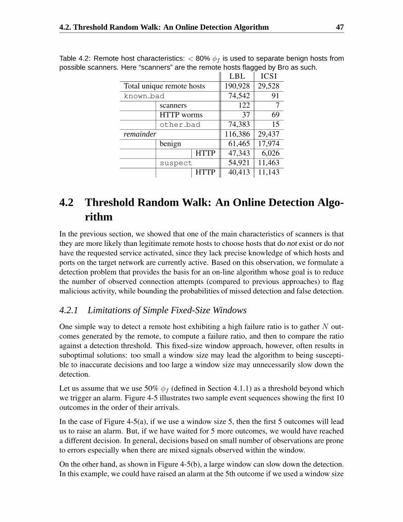
4.2. Threshold Random Walk: An Online Detection Algorithm 47
Table 4.2: Remote host characteristics: < 80% φf is used to separate benign hosts frompossible scanners. Here “scanners” are the remote hosts flagged by Bro as such.
LBL ICSITotal unique remote hosts 190,928 29,528known bad 74,542 91
scanners 122 7HTTP worms 37 69other bad 74,383 15
remainder 116,386 29,437benign 61,465 17,974
HTTP 47,343 6,026suspect 54,921 11,463
HTTP 40,413 11,143
4.2 Threshold Random Walk: An Online Detection Algo-rithm
In the previous section, we showed that one of the main characteristics of scanners is thatthey are more likely than legitimate remote hosts to choose hosts that do not exist or do nothave the requested service activated, since they lack precise knowledge of which hosts andports on the target network are currently active. Based on this observation, we formulate adetection problem that provides the basis for an on-line algorithm whose goal is to reducethe number of observed connection attempts (compared to previous approaches) to flagmalicious activity, while bounding the probabilities of missed detection and false detection.
4.2.1 Limitations of Simple Fixed-Size Windows
One simple way to detect a remote host exhibiting a high failure ratio is to gather N out-comes generated by the remote, to compute a failure ratio, and then to compare the ratioagainst a detection threshold. This fixed-size window approach, however, often results insuboptimal solutions: too small a window size may lead the algorithm to being suscepti-ble to inaccurate decisions and too large a window size may unnecessarily slow down thedetection.
Let us assume that we use 50% φf (defined in Section 4.1.1) as a threshold beyond whichwe trigger an alarm. Figure 4-5 illustrates two sample event sequences showing the first 10outcomes in the order of their arrivals.
In the case of Figure 4-5(a), if we use a window size 5, then the first 5 outcomes will leadus to raise an alarm. But, if we have waited for 5 more outcomes, we would have reacheda different decision. In general, decisions based on small number of observations are proneto errors especially when there are mixed signals observed within the window.
On the other hand, as shown in Figure 4-5(b), a large window can slow down the detection.In this example, we could have raised an alarm at the 5th outcome if we used a window size

48 Chapter 4. Portscan Detection
F S F S F S S S S S60%
(a) Window size: 5
F F SF FFFFF S80%
(b) Window size: 10
Figure 4-5: Detections based on fixed-size windows: F represents a failure event and S asuccess event.
5. Basically, when the evidence observed so far strongly favors one model over the other,waiting to see more data does not increase a confidence level much and it is often better toterminate the observation now for faster detection.
Following sections show that our detection approach, which is built on the framework of thesequential hypothesis testing (see Chapter 2.2 for the review) overcomes the limitations ofthe simple fixed-size windows and dynamically adjusts a window size based on the strengthof evidence observed.
4.2.2 Model
Let an event be generated when a remote source r makes a connection attempt to a localdestination l. We classify the outcome of the attempt as either a “success” or a “failure”,where the latter corresponds to a connection attempt to an inactive host or to an inactiveservice on an otherwise active host.
For a given r, let Yi be a random (indicator) variable that represents the outcome of the firstconnection attempt by r to the ith distinct local host, where
Yi =
{
0 if the connection attempt is a success1 if the connection attempt is a failure
As outcomes Y1, Y2, . . . , are observed, we wish to determine whether r is a scanner. Intu-itively, we would like to make this detection as quickly as possible, but with a high proba-bility of being correct. Since we want to make our decision in real-time as we observe theoutcomes, and since we have the opportunity to make a declaration after each outcome, thedetection problem is well suited for the method of sequential hypothesis testing developedby Wald in his seminal work [80].
We consider two hypotheses, H0 and H1, where H0 is the hypothesis that the given remotesource r is benign and H1 is the hypothesis that r is a scanner. Let us now assume that,conditional on the hypothesis Hj , the random variables Yi|Hj i = 1, 2, . . . are independentand identically distributed (i.i.d.). Then we can express the distribution of the Bernoulli

4.2. Threshold Random Walk: An Online Detection Algorithm 49
random variable Yi as:
Pr[Yi = 0|H0] = θ0, Pr[Yi = 1|H0] = 1− θ0
Pr[Yi = 0|H1] = θ1, Pr[Yi = 1|H1] = 1− θ1 (4.1)
The observation that a connection attempt is more likely to be a success from a benignsource than a malicious one implies the condition:
θ0 > θ1.
The goal of the real-time detection algorithm is to make an early decision as an event streamarrives to the system while satisfying the performance conditions (2.1). As discussed inChapter 2.2, upon each event’s arrival, we calculate the likelihood ratio:
Λ(Y) ≡ Pr[Y|H1]
Pr[Y|H0]= Πn
i=1
Pr[Yi|H1]
Pr[Yi|H0](4.2)
, where Y is the vector of events observed so far and Pr[Y|Hi] represents the conditionalprobability mass function of the event stream Y given that model Hi is true; and where thesecond equality in (4.2) follows from the i.i.d. assumption. The decision-making processis illustrated in Figure 2-1.
Essentially, we are modeling a random walk for which the excursion probabilities comefrom one of two possible sets of probabilities, and we seek to identify which set is mostlikely responsible for an observed walk. We call our algorithm TRW, Threshold RandomWalk, since our decision-making process corresponds to a random walk with two thresh-olds.4
As we will show in Section 4.2.4, while the Bernoulli distributions conditioned on hypothe-ses H0 and H1 play no role in the selection of the thresholds η1 and η0, they do (along withthe thresholds) strongly affect N , the number of observations until the test terminates, i.e.,until one of the hypotheses is selected.
4.2.3 Numerical Analysis
In order to assess the impact of approximate solutions for η0 and η1 (2.5) on the algorithmperformance, we conducted numerical analysis varying parameters, α, β, θ0, and θ1. At theend of the simulation, we calculated achieved PF and PD and compared them with α andβ to see whether the approximate solution for η0 and η1 allowed the algorithm to meet theperformance criteria.
At each iteration, i, a random number, Ri, is generated from a uniform distribution U(0, 1).Given α and β, two thresholds, η0 and η1 are calculated using Equation (2.5). Ri is usedto determine whether this sample observation represents a failed event or successful event.If the simulation is to evaluate the detecting probability of scanners (benign users), Ri is
4To be more precise, it is a random walk in the logarithm of the likelihood ratio space.

50 Chapter 4. Portscan Detection
compared to Pr[Yi = 0|H1] = θ1 (Pr[Yi = 0|H0] = θ0) and we regard the event as asuccess if Ri is less than a priori probability, θ1 (θ0).
Starting from 1, the likelihood ratio, Λ is updated as an event is generated. The decision ismade at the point where Λ is greater than η1 or less than η0. This process is repeated untilit accomplishes M decisions.
Figure 4-6 shows that regardless of a priori probabilities, θ0 and θ1, the performance goalis achieved when Equation (2.5) is used to set η0 and η1. It also shows that as θ1 getscloser to θ0, the performance goes down, but not lower than a target performance. Thissimulation result suggests the choice of a priori probabilities, θ1 and θ0 has little affect onthe performance and the result still maintains the performance criteria. However, as wewill show in the next section, a priori probabilities do affect the number of observationsrequired to reach a decision and in practice, this can affect the performance since we cannot always expect that such a large number of events are available for decision.
Figures 4-7(a) and 4-7(b) show the selected 100 steps during the simulations for detectingscanners or benign users. In both cases, β = 0.99, α = 0.01, θ0 = 0.9, and θ1 = 0.2
For scanners, it requires at least three observations to reach a decision and the averagenumber of observations is 4.110 when the simulation was done for 10,000 scanners. Outof 10,000 scanners, only 33 were detected as benign users, thus the resulting detectionprobability is 0.9967. Figure 4-7(a) shows the case for a false negative at around the 1760th
step where 4 consecutive successes happened for this particular scanner. The probabilityfor this rare event is 0.24 = 0.0016.
For benign users, it requires at least four observations to reach a decision and the averagenumber of observations is 5.011 when the simulation was done for 10,000 benign cases.Out of 10,000 cases, 48 were decided as scanners, thus the resulting false positive proba-bility is 0.0048. Figure 4-7(b) shows the case for a false positive at around the 860th stepwhere 3 failures within 4 trials happened for this particular benign user. The probabilityfor this event is 0.13 × 0.9 = 0.009.
4.2.4 Number of Observations to Select Hypothesis
Given the performance criteria, (2.1), and the associated thresholds, (2.5), the remainingquantity of interest is the number of observation N until the test terminates, i.e., until oneof the hypotheses is selected. Following Wald [80], we present approximate expressionsfor the expected value of N and the tail probability of N .
For the analysis of N , it is convenient to consider the log of the likelihood ratio, (4.2), andview the resulting expression as a random walk:
SN ≡ ln(Λ(Y)) =N∑
i=1
Xi, where Xi ≡ ln
(
Pr[Yi|H1]
Pr[Yi|H0]
)
, and N is the observation number at which SN first hits or crosses either the upper thresh-old, ln η1, or lower threshold, ln η0. (Note that S0 = 0.)

4.2. Threshold Random Walk: An Online Detection Algorithm 51
0.9
0.91
0.92
0.93
0.94
0.95
0.96
0.97
0.98
0.99
1
0.9 0.91 0.92 0.93 0.94 0.95 0.96 0.97 0.98 0.99 1 0.9
0.91
0.92
0.93
0.94
0.95
0.96
0.97
0.98
0.99
1
PD
β
θ1=0.2θ1=0.5θ1=0.8
y=x
(a) Actual detection rate (PD) vs. target detection rate (β) : The targetfalse positive rate (α) is set to 0.01 and θ0 to 0.9.
0
0.02
0.04
0.06
0.08
0.1
0 0.02 0.04 0.06 0.08 0.1 0
0.02
0.04
0.06
0.08
0.1
0.12
PF
α
θ1=0.2θ1=0.5θ1=0.8
y=x
(b) Actual false positive rate (PF ) vs. target false positive rate (α) : Thetarget detection rate (β) is set to 0.99 and θ0 to 0.9.
Figure 4-6: Achieved performance as a function of a target performance: Each dot in theplots is a simulation result (PD or PF ) as we vary a target performance (β or α). Thesimulation result is obtained after M = 100, 000 random numbers are generated. y = x isa reference line indicating that a resulting performance is equal to a target performance.

52 Chapter 4. Portscan Detection
From Wald’s equality, E[N ] = E[SN ]/E[Xi], and we can obtain expressions for E[SN ] andE[Xi], conditioned on the hypotheses H0 and H1. Then, using the central limit theorem, weprovide the tail probability of N , which can be useful to estimate the worst case scenarioswhen this algorithm is used.
For Xi,
Xi|H0 =
{
ln 1−θ1
1−θ0
with prob. 1− θ0
ln θ1
θ0
with prob. θ0
Xi|H1 =
{
ln 1−θ1
1−θ0
with prob. 1− θ1
ln θ1
θ0
with prob. θ1
E[Xi|H0] = (1− θ0) ln1− θ1
1− θ0
+ θ0 lnθ1
θ0
(4.3)
E[Xi|H1] = (1− θ1) ln1− θ1
1− θ0
+ θ1 lnθ1
θ0
If we assume the sequential test ends with SN hitting, equaling, either ln η0 or ln η1, i.e., ifwe ignore any overshoot, then
SN |H0 =
{
ln η1 with prob. αln η0 with prob. 1− α
SN |H1 =
{
ln η1 with prob. βln η0 with prob. 1− β
E[SN |H0] = α ln η1 + (1− α) ln η0 (4.4)E[SN |H1] = β ln η1 + (1− β) ln η0
Combining (2.5), (4.3), and (4.4), we obtain the approximate result in Equation (4.5).
E[N |H0] =α ln β
α+ (1− α) ln 1−β
1−α
θ0 ln θ1
θ0
+ (1− θ0) ln 1−θ1
1−θ0
(4.5)
E[N |H1] =β ln β
α+ (1− β) ln 1−β
1−α
θ1 ln θ1
θ0
+ (1− θ1) ln 1−θ1
1−θ0
For the tail probability of N , we apply the central limit theorem to∑
i=1 Xi. Note that ifthe random walk,
∑no
i=1 Xi is greater than or equal to upper threshold ln η1 at observationno, then the sequential hypothesis test must have terminated by then, i.e., N ≤ no. Condi-tioning on the hypothesis for which hitting the upper threshold is more likely, H1, we have:

4.2. Threshold Random Walk: An Online Detection Algorithm 53
Pr[no∑
i=1
Xi ≥ ln η1|H1] ≤ Pr[N ≤ no|H1] (4.6)
Normalizing the left hand side of (4.6) to mean zero variance one, yields:
Pr
[∑no
i=1 Xi − noE[Xi|H1]√no · σ(Xi|H1)
≥ ln η1 − noE[Xi|H1]√no · σ(Xi|H1)
|H1
]
(4.7)
, where σ(Xi|Hj) denotes the standard deviation of Xi given hypothesis Hj , j = 0, 1.
σ(Xi|H0) =√
θ0(1− θ0) · ln(
1− θ1
1− θ0
θ0
θ1
)
σ(Xi|H1) =√
θ1(1− θ1) · ln(
1− θ1
1− θ0
θ0
θ1
)
Applying the central limit theorem to (4.7) yields an approximate lower bound for the dis-tribution of N |H1, which can be used as an approximation for the distribution itself, wherethe error tends to be on the conservative side (i.e., tends to under estimate the likelihoodN ≤ no). Thus,
Pr[N ≤ no|H1] ≈ 1 − Φ
(
ln η1 − noE[Xi|H1]√no · σ(Xi|H1)
)
(4.8)
, where Φ(x) equals the probability of a normally distributed random variable with meanzero and variance one being less than or equal to x.
Analogous reasoning for the lower threshold and conditioning on H0 yields
Pr[N ≤ no|H0] ≈ Φ
(
ln η0 − noE[Xi|H0]√no · σ(Xi|H0)
)
(4.9)
4.2.5 Discussions on E[N |H1] vs. θ0 and θ1
As shown in Equation (4.5), E[N |H0] and E[N |H1] are a function of the four parameters,α, β, θ0, and θ1, the false positive and detection probabilities, and the degree to whichscanners differ from benign hosts in terms of modeling their probability of making failedconnections. With those values set, we can estimate the average number of distinct destina-tion IP addresses that a given port scanner can probe before being caught by the algorithm.
Assuming a scanner picks IP addresses at random, θ1—the probability that it chooses anIP address with the requested service on—depends on the density of these servers in amonitored network. Figure 4-8(a) shows how E[N |H1] changes as θ1 increases. Withα = 0.01, β = 0.99, and θ0 = 0.8, E[N |H1] is 5.4 when θ1 = 0.2, and goes up to11.8 when θ1 = 0.4 (we used θ1 = 0.2 based on the observations from data analysis inSection 4.1.) In general, it takes longer to tell one model from the other the closer the two

54 Chapter 4. Portscan Detection
models are to each other. Figure 4-8(a) also shows that E[N |H1] goes up as α gets lower,which illustrates the trade off between low false positive probability and fast detection.We can detect faster in situations where θ0 is higher. Legitimate users often make a connec-tion request with a host name. Unless the DNS provides outdated information, they rarelyaccess inactive servers, and therefore θ0—the probability that those users hit an active IPaddress—can be fairly high. However, the presence of benign Web crawlers and prox-ies that sometimes access inactive servers through broken links, or a few infected clientsputting requests through a proxy that serves mostly benign users, can require a lower θ0 formodeling.In those circumstances where such problematic hosts can be controlled, however, then wecan configure the detection algorithm to use a higher θ0, and thus enable it to make a fasterdecision. Figure 4-8(b) shows E[N |H1] when θ0 is set to 0.9. The decrease in detectiontime is significant.In practice, one can tune θ1 based on the density of the most popular service within anaddress space and then set θ0 to a value reasonably higher than θ1. However, for somenetworks where most addresses are allocated and running the same kind of service all thetime, the little difference between θ1 and θ0 will render TRW less effective.
4.2.6 Limitations
We develop TRW based on the assumption that conditional on the hypothesis (that a re-mote host is benign or a scanner), any two distinct connection attempts will have the samelikelihood of succeeding and their chances of success are unrelated to each other.The bounds for upper and lower thresholds, Equations (2.3) and (2.4), are valid, given thatthe sequential hypothesis test will eventually terminate with probability one, which holdsgiven independence of outcomes, and also for some cases of dependence [80]. Unfortu-nately, this will not hold for all cases of dependence. For instance, if a scanner probesN inactive servers exactly alternating with N active servers, our random walk will oscil-late between one step up and one step down and it will never hit either threshold whenθ1 + θ0 = 1. An informed attacker can evade TRW exploiting this dependence if he inter-leaves scan traffic with the traffic to N active hosts.On the other hand, dependence that leads to positive correlation in outcomes (i.e., successesare more likely to be followed by another success or likewise for failures) will tend toshorten the time to hit a threshold. This form of dependence seems more likely to occur inpractice.Dependence, however, invalidates the second equality in Equation (4.2). Instead, the like-lihood ratio should be calculated using a joint probability distribution, which complicatesthe computation.
4.3 EvaluationThis section evaluates the performance of the TRW algorithm in terms of its accuracyand the detection speed using trace-driven simulations. We explicate cases flagged as H0

4.3. Evaluation 55
(benign) or H1 (malicious) by TRW. Then, we compare the performance of TRW with thatof Bro and Snort.
4.3.1 Trace-driven Simulation
We use the datasets described in Section 4.1 for evaluation. Each line in a dataset representsa connection seen by the Bro NIDS, sorted by the timestamp of the first packet belongingto the connection. Connection information includes a source IP, s, a destination IP, d, andthe connection status. In reality, the connection status is not immediately available whenthe first packet arrives. For our analysis, we assume that the detector can consult an oraclethat can tell upon seeing an incoming TCP SYN whether it will result in an established,rejected, or unanswered connection. (We might approximate such an oracle by giving thedetector access to a database of which ports are open on which addresses, though “churn”at a site might make maintaining the database problematic.) Alternatively, the detectorcan wait a short period of time to see whether the SYN elicits a SYN ACK, a RST, or noresponse, corresponding to the three cases above.
For each s, TRW maintains 3 variables. Ds is the set of distinct IP addresses to which s haspreviously made connections. Ss reflects the decision state, one of: PENDING; H0; or H1.Ls is the likelihood ratio. For each line in the dataset, the simulation executes the followingsteps:
1) Skip the line if Ss is not PENDING (a decision has already made for the remote hosts).
2) Determine whether the connection is successful or not. A connection is consideredsuccessful if it elicited a SYN ACK.5
3) Check whether d already belongs to Ds. If so, skip the next steps and proceed tothe next connection. Update Ds with d, and update the likelihood ratio, Ls usingEquation (4.2).
5) If Ls equals or exceeds η1, set Ss to H1. If Ls is lower than or equal to η0, set Ss toH0.
Table 4.3 shows the simulation results for LBL and ICSI datasets. The results depend onthe parameter values; we present here results based on typical settings, where the detectionprobability (α) should be at least 0.99 and the false alarm rate (β) no larger than 0.01. Wechose θ1 = 0.2 and θ0 = 0.8 based on the discussion in Section 4.1. Although we found
5Due to ambiguities in Bro’s log format, for connections terminated by the remote originator with aRST we sometimes cannot determine whether the local host actually responded. Bro generates the sameconnection status for the case in which the connection was first established via the local host responding witha SYN ACK and the case where the remote host sent a SYN and then later, without receiving any reply, senta RST. Accordingly, we treat such connections as failures if the logs indicate the local host did not send anydata to the remote host.
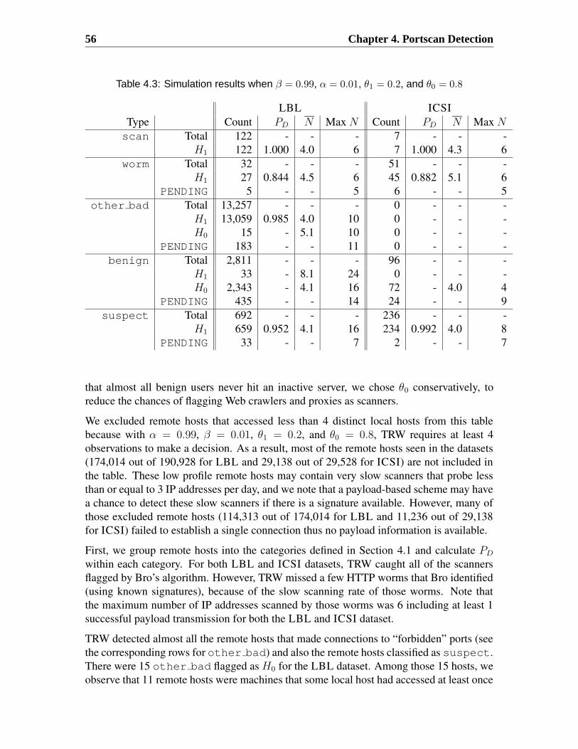
56 Chapter 4. Portscan Detection
Table 4.3: Simulation results when β = 0.99, α = 0.01, θ1 = 0.2, and θ0 = 0.8
LBL ICSIType Count PD N Max N Count PD N Max Nscan Total 122 - - - 7 - - -
H1 122 1.000 4.0 6 7 1.000 4.3 6worm Total 32 - - - 51 - - -
H1 27 0.844 4.5 6 45 0.882 5.1 6PENDING 5 - - 5 6 - - 5
other bad Total 13,257 - - - 0 - - -H1 13,059 0.985 4.0 10 0 - - -H0 15 - 5.1 10 0 - - -
PENDING 183 - - 11 0 - - -benign Total 2,811 - - - 96 - - -
H1 33 - 8.1 24 0 - - -H0 2,343 - 4.1 16 72 - 4.0 4
PENDING 435 - - 14 24 - - 9suspect Total 692 - - - 236 - - -
H1 659 0.952 4.1 16 234 0.992 4.0 8PENDING 33 - - 7 2 - - 7
that almost all benign users never hit an inactive server, we chose θ0 conservatively, toreduce the chances of flagging Web crawlers and proxies as scanners.
We excluded remote hosts that accessed less than 4 distinct local hosts from this tablebecause with α = 0.99, β = 0.01, θ1 = 0.2, and θ0 = 0.8, TRW requires at least 4observations to make a decision. As a result, most of the remote hosts seen in the datasets(174,014 out of 190,928 for LBL and 29,138 out of 29,528 for ICSI) are not included inthe table. These low profile remote hosts may contain very slow scanners that probe lessthan or equal to 3 IP addresses per day, and we note that a payload-based scheme may havea chance to detect these slow scanners if there is a signature available. However, many ofthose excluded remote hosts (114,313 out of 174,014 for LBL and 11,236 out of 29,138for ICSI) failed to establish a single connection thus no payload information is available.
First, we group remote hosts into the categories defined in Section 4.1 and calculate PD
within each category. For both LBL and ICSI datasets, TRW caught all of the scannersflagged by Bro’s algorithm. However, TRW missed a few HTTP worms that Bro identified(using known signatures), because of the slow scanning rate of those worms. Note thatthe maximum number of IP addresses scanned by those worms was 6 including at least 1successful payload transmission for both the LBL and ICSI dataset.
TRW detected almost all the remote hosts that made connections to “forbidden” ports (seethe corresponding rows for other bad) and also the remote hosts classified as suspect.There were 15 other bad flagged as H0 for the LBL dataset. Among those 15 hosts, weobserve that 11 remote hosts were machines that some local host had accessed at least once
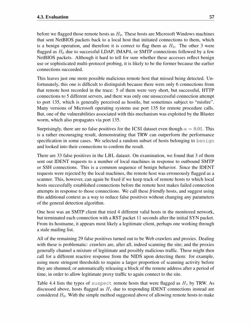
4.3. Evaluation 57
before we flagged those remote hosts as H0. These hosts are Microsoft Windows machinesthat sent NetBIOS packets back to a local host that initiated connections to them, whichis a benign operation, and therefore it is correct to flag them as H0. The other 3 wereflagged as H0 due to successful LDAP, IMAP4, or SMTP connections followed by a fewNetBIOS packets. Although it hard to tell for sure whether these accesses reflect benignuse or sophisticated multi-protocol probing, it is likely to be the former because the earlierconnections succeeded.
This leaves just one more possible malicious remote host that missed being detected. Un-fortunately, this one is difficult to distinguish because there were only 6 connections fromthat remote host recorded in the trace: 5 of them were very short, but successful, HTTPconnections to 5 different servers, and there was only one unsuccessful connection attemptto port 135, which is generally perceived as hostile, but sometimes subject to “misfire”.Many versions of Microsoft operating systems use port 135 for remote procedure calls.But, one of the vulnerabilities associated with this mechanism was exploited by the Blasterworm, which also propagates via port 135.
Surprisingly, there are no false positives for the ICSI dataset even though α = 0.01. Thisis a rather encouraging result, demonstrating that TRW can outperform the performancespecification in some cases. We selected a random subset of hosts belonging to benignand looked into their connections to confirm the result.
There are 33 false positives in the LBL dataset. On examination, we found that 3 of themsent out IDENT requests to a number of local machines in response to outbound SMTPor SSH connections. This is a common sequence of benign behavior. Since the IDENTrequests were rejected by the local machines, the remote host was erroneously flagged as ascanner. This, however, can again be fixed if we keep track of remote hosts to which localhosts successfully established connections before the remote host makes failed connectionattempts in response to those connections. We call these friendly hosts, and suggest usingthis additional context as a way to reduce false positives without changing any parametersof the general detection algorithm.
One host was an SMTP client that tried 4 different valid hosts in the monitored network,but terminated each connection with a RST packet 11 seconds after the initial SYN packet.From its hostname, it appears most likely a legitimate client, perhaps one working througha stale mailing list.
All of the remaining 29 false positives turned out to be Web crawlers and proxies. Dealingwith these is problematic: crawlers are, after all, indeed scanning the site; and the proxiesgenerally channel a mixture of legitimate and possibly malicious traffic. These might thencall for a different reactive response from the NIDS upon detecting them: for example,using more stringent thresholds to require a larger proportion of scanning activity beforethey are shunned; or automatically releasing a block of the remote address after a period oftime, in order to allow legitimate proxy traffic to again connect to the site.
Table 4.4 lists the types of suspect remote hosts that were flagged as H1 by TRW. Asdiscussed above, hosts flagged as H1 due to responding IDENT connections instead areconsidered H0. With the simple method suggested above of allowing remote hosts to make

58 Chapter 4. Portscan Detection
Table 4.4: Break-down of “suspects” flagged as H1
Type LBL ICSIIDENT 18 (2.7%) 0 (0%)
≥ 2 protocols 87 (13.2%) 8 (3.4%)only HTTP 541 (82.1%) 226 (96.6%)remainder 13 (2.0%) 0 (0%)
failed connections if they’ve previously received outbound connections from the site, wewere able to confirm that all of the 18 suspect remote hosts were flagged due to re-sponding IDENT connection for the LBL dataset. Over 80% made nothing but failedHTTP connections, and we therefore suspect them as undetected worms.
Table 4.3 also shows the average (N ) and maximum number of distinct local IP addressesthat each detected remote host accessed upon being flagged. In theory, when α = 0.01,β = 0.99, θ0 = 0.8, and θ1 = 0.2, the approximate solution for E[N |H1] is 5.4 as shownin Section 4.2.5, and our trace-driven simulations are consistent with this figure. Thissuggests that the parameters chosen for θ0 and θ1 adequately model the actual behaviors ofscanners and benign users. Note that with everything else fixed, N would have been muchhigher than 5 if θ1 was greater than 0.3, as shown in Figure 4-8(a). It is also noteworthythat even in the worst case, a decision was made before a scanner probed more than 16machines—strictly better than the best case provided by Bro’s algorithm.
Table 4.5: Performance in terms of efficiency and effectiveness: Post-filtering eliminatesremotes to which a local host previously connected. Pre-filtering is calculated based onTable 4.3.
Trues H1 True positives Efficiency EffectivenessLBL Pre-filtering 14,103 13,900 13,867 0.998 0.983
Post-filtering 14,068 13,878 13,848 0.998 0.984ICSI Pre-filtering 294 286 286 1.000 0.973
Post-filtering 294 286 286 1.000 0.973
Finally, to quantify the effectiveness of TRW, we use the two measures proposed by Stani-ford et al. [66]:
• Efficiency: the ratio of the number of detected scanners (true positives) to all casesflagged as H1.
• Effectiveness: the ratio of the number of true positives to all scanners (trues). This isthe same as PD, detection rate.
Efficiency conveys a similar meaning to false positive rate, but is more useful when the totalnumber of true positives is significantly smaller than the total number of samples. Table 4.5

4.3. Evaluation 59
Table 4.6: Comparison of the number of H1 across three categories for LBL dataset
TRW Bro SnortType Total H1 N Max N H1 N Max N H1 N Max Nscan 121 121 4.0 6 121 21.4 28 63 16.8 369
benign 2811 30 - - 0 - - 57 - -suspect 692 659 4.1 16 0 - - 28 7.9 33
Table 4.7: Comparison of the number of H1 across three categories for ICSI dataset
TRW Bro SnortType Total H1 N Max N H1 N Max N H1 N Max Nscan 7 7 4.3 6 7 35.9 119 5 6.0 6
benign 96 0 - - 0 - - 0 - -suspect 236 234 4.0 8 0 - - 2 6.0 6
shows these values for the two sites. For ICSI, because of 8 misses (6 HTTP worms and 2suspect), TRW results in a lower effectiveness (0.973) than expected (β = 0.99). But,the overall performance is excellent. We compare TRW’s performance with that of Bro andSnort in the next section.
4.3.2 Comparison with Bro and Snort
For simplicity, we exclude the worm and other bad category because as configured atLBL and ICSI, Bro does not perform scan-detection analysis for these. As throughout thechapter, we configure Bro’s algorithm with N = 20 distinct hosts.
For Snort, we consider its portscan2 scan-detection preprocessor, which takes into ac-count distinct connections rather than distinct TCP SYN packets—the latter can generatemany false positives if a single host sends multiple SYNs in the same failed connectionattempt. We use Snort’s default settings, for which it flags a source IP address that hassent connections to 5 different IP addresses within 60 seconds. (We ignore Snort’s rule for20-different-ports-within-60-seconds because our emphasis here is on detecting scans ofmultiple hosts rather than vertical scans of a single host.) We note that Snort’s algorithmcan erroneously flag Web crawlers or any automated process to fetch Web documents ifthere are more than 5 active Web servers in a monitored network. It can also be easilyevaded by a scanner who probes a network no faster than 5 addresses/minute. Tables 4.6and 4.7 show the number of (non-local) hosts reported as H1 by the three algorithms.
Table 4.8 compares the efficiency and effectiveness across the three algorithms for bothdatasets. Note that two measures for TRW differ from Table 4.5 because of the two cate-gories (worm, other bad) excluded in this comparison. Bro has the highest efficiencyfollowed by TRW and Snort. But Bro’s highest efficiency comes at a cost of low effective-ness. Given its simple thresholds and limited time window, we expected that Snort would

60 Chapter 4. Portscan Detection
Table 4.8: Comparison of the efficiency and effectiveness across TRW, Bro, and Snort
Trace Measures TRW Bro SnortLBL Efficiency 0.963 1.000 0.615
Effectiveness 0.960 0.150 0.126N 4.08 21.40 14.06
ICSI Efficiency 1.000 1.000 1.000Effectiveness 0.992 0.029 0.029
N 4.06 36.91 6.00
provide fast detection. But, as shown in Tables 4.6 and 4.7, Snort was slower than TRWon average. In contrast to TRW, which on average flagged scanners when they hit no morethan 5 distinct IP addresses, Snort waited for more than 13 IP addresses. Snort can increasethe detection speed by lowering Y or Z values.6 But, this will likely increase false alarms.Indeed, for LBL, 38.5% of the alarms by Snort were due to false positives.
Compared with Snort and Bro, TRW provided the highest effectiveness while maintaininghigher than 0.96 efficiency. On average, detection was made when a target made connec-tions to 4.1 active or inactive IP addresses. This average number of give-away IP addressesto scanners or suspects is about 3 times lower than that of Snort and about 5 timeslower than that of Bro. In addition, TRW has the advantage over Snort that its analysis isnot confined to a limited window of time: TRW has a wide dynamic range.
4.4 Discussion
In this section we look at a number of additional dimensions to the problem space andsketch our thinking on how each one can be pursued.
Leveraging Additional Information. TRW’s performance is somewhat remarkable giventhe limited information it uses. Potential refinements include: (1) factoring in the specificservice (for example, we could use more conservative parameters for possible HTTP scan-ning than for other ports, given the difficulty of confusing HTTP scanners with HTTP prox-ies); (2) distinguishing between unanswered connection attempts and rejected connectionattempts, as the former might be more indicative of a complete “shot in the dark” whereasthe latter could sometimes indicate a service that is temporarily off-line; (3) consideringthe time duration that a local address has been inactive, to be robust to benign connectionattempts made to temporarily unavailable hosts; (4) considering the rate at which a remotehost makes connection attempts (see Chapter 6); (5) introducing a component of correla-tion in the model, e.g., that two consecutive failed connection attempts are more suspectthan two failures separated by a success; (6) devising a model of which local addresses andports are historically more likely to be visited by benign sources or scanners.
6See Section 3.1.1 for the definitions of Y and Z: Snort raises an alarm if a given source IP addresscontacted more than X number of ports or Y number of IP addresses in Z seconds.

4.4. Discussion 61
However, incorporating information such as the above is a two-edged sword. It may provideadditional detection power—something to keep in mind for the discussion of other issuesin this section—but at the cost of complicating use of the model, analysis of its properties,and, potentially, undermining its performance in some situations.
Managing State. The need to track for each remote host the different local addresses towhich it has connected can in fact require a large amount of state. For example, imagine theoperation of the algorithm during a SYN flooding attack with spoofed remote addresses.Virtually every arriving SYN will require the instantiation of state to track the new pur-ported remote host. If, however, we cap the state available to the detector, then an attackercan launch a flood in order to exhaust the state, and then conduct a concurrent scan withimpunity.
How to Respond. As shown in Section 4.3, TRW is much more effective at detectinglow-volume scanners than Bro or Snort. However, this then raises the question of what todo with the alerts. For example, Table 4.5 shows that TRW detects nearly 14,000 scan-ners in the LBL dataset (presumably almost all of these are worms), vastly more than the122 detected by Bro at the site. As mentioned in the Introduction, LBL uses Bro’s scannerdetection decisions to trigger blocking of the hostile remote host. However, the site reportsthat the blocking mechanism cannot scale to 1000’s of blocks per day (this is why the sitedoes not block HTTP scanners, because at times the endemic HTTP scans from wormscan reach such levels). Thus, there is future work needed on mechanisms for determiningwhether a particular scanner is “block-worthy,” i.e., will the given scanner continue to scanto a degree significant enough that they merit blocking or some form of rate control, orcan they be ignored because they are scanning at a rate (or for a service of sufficiently lowinterest) that the site can afford to let the scan run its course?
Evasion and Gaming. Any scan detection algorithm based on observing failed connectionattempts is susceptible to manipulation by attackers who spoof remote addresses and causeinnocent remote hosts to be penalized. Depending on the reactive response taken when ascan is detected, address spoofing could provide the attacker with a great deal of leveragefor denial-of-service. We note that the operators at LBL recognize this risk, and addressit using “white lists” of critical remote hosts that should never be blocked. They havefound this approach practical in today’s environment, but this could change in the future ifattackers become more energetic in targeting the response system. A possible additionalapproach here would be to have a honeypot respond to some of the connection attemptsto see whether the remote host then completes the 3-way establishment handshake. If not,then the remote address is potentially spoofed.
Another issue concerns ways for an attacker to evade detection. For TRW, this is not sodifficult. An attacker could compile a list of known servers at a site (running services otherthan those of interest to them) and then intermingle connection attempts to those with thewider connection attempts of a true scan. The successes of the camouflage connectionswould then drive the random walk away from an H1 decision. Countering this threat re-quires either incorporating service information (as discussed above) or modeling whichcombinations of addresses legitimate users tend to access, and then giving less weight tosuccessful connections not fitting with these patterns.

62 Chapter 4. Portscan Detection
Distributed Scans. As stated in the Introduction, we confined our work to the problem ofdetermining whether a single remote address corresponds to a malicious scanner. It appearsdifficult to directly adapt our framework to determining whether a set of remote addressescollectively correspond to malicious scanning (such as if they divide up the address spaceand each probe just a couple of addresses within it), because our algorithm depends ontracking success/failure information of individual remotes. It may, however, be possible toextend our algorithm with post processing to try to do so by combining a number of “lowgrade” signals (either detected scanners, or those whose random walks have taken themsomewhat in the direction of H1).
4.5 Summary
We have presented the development and evaluation of TRW—Threshold Random Walk—analgorithm to rapidly detect portscanners based on observations of whether a given remotehost connects successfully or unsuccessfully to newly-visited local addresses. TRW ismotivated by the empirically-observed disparity between the frequency with which suchconnections are successful for benign hosts vs. for known-to-be malicious hosts. The un-derpinnings of TRW derive from the theory of sequential hypothesis testing, which allowsus to establish mathematical bounds on the expected performance of the algorithm.
Using an analysis of traces from two qualitatively different sites, we show that TRW re-quires a much smaller number of connection attempts (4 or 5 in practice) to detect maliciousactivity compared to previous schemes used by the Snort and Bro NIDS. TRW has the ad-ditional properties that (1) even though it makes quick decisions, it is highly accurate, withvery few false positives, and (2) it is conceptually simple, which leads to both comprehen-sibility regarding how it works, and analytic tractability in deriving theoretical bounds onits performance.
In summary, TRW performs significantly faster and also more accurately than other currentsolutions.
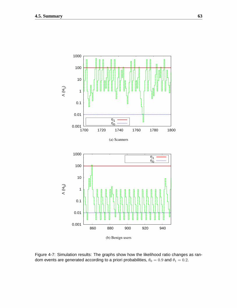
4.5. Summary 63
0.001
0.01
0.1
1
10
100
1000
1700 1720 1740 1760 1780 1800
Λ (
H1)
η1η0
(a) Scanners
0.001
0.01
0.1
1
10
100
1000
860 880 900 920 940
Λ (
H0)
η1η0
(b) Benign users
Figure 4-7: Simulation results: The graphs show how the likelihood ratio changes as ran-dom events are generated according to a priori probabilities, θ0 = 0.9 and θ1 = 0.2.

64 Chapter 4. Portscan Detection
2
4
6
8
10
12
14
16
18
0 0.05 0.1 0.15 0.2 0.25 0.3 0.35 0.4 2
4
6
8
10
12
14
16
18E
[N|H
1]
θ1
α= 0.001α = 0.005
α = 0.01
(a) θ0 = 0.8
2
4
6
8
10
12
14
16
18
0 0.05 0.1 0.15 0.2 0.25 0.3 0.35 0.4 2
4
6
8
10
12
14
16
18
E[N
|H1]
θ1
α= 0.001α = 0.005
α = 0.01
(b) θ0 = 0.9
Figure 4-8: E[N |H1] vs. other parameters; β is fixed to 0.99

Chapter 5
Detection of Scanning Worm Infections
Network worms propagate to other hosts on the Internet via many methods: by searchingthe IPv4 address space (scanning worms); by searching the file system of an infected hostfor addresses that the infected host has already contacted (topological worms); by usingthe hist-lists of susceptible hosts identified by earlier scans (flash worms); or by queryingspecific servers for the addresses of potential victim hosts (meta-server worms). See [82]by Weaver et al. for more discussions of a taxonomy of network worms.
Among these propagation methods, scanning has been most frequently employed by theworms that have been released in the past few years. At its simplest, a scanning wormchooses its next victim by randomly drawing from the 232 IPv4 addresses and transmits amalicious payload if the victim accepts a connection request [44, 45, 59]. A few variationswere adapted by later worms in order to speed up the infection spread: Code Red II [11]and Sasser [73] probe local hosts that are in the same subnet as the infected machine moreoften than a completely random IP address. The Blaster worm [24] sequentially probeshosts starting from an IP address picked at random, with a bias toward local addresses onthe same subnet.
The efficiency of scanning depends on the density of targeted vulnerable hosts on the Inter-net, which can be quite low for several reasons. First of all, more than 38% of IPv4 addressblocks are not allocated to any registries [29], and therefore no hosts are reachable via thoseIP addresses. Second, many networks employ a firewall, which blocks incoming packets tocertain ports that are known to be vulnerable to many existing exploits (e.g., TCP ports 135and 139 corresponding to Windows RPC and NetBIOS). Finally, when a worm is fortunateenough to find an active host, the chosen host may not be running the targeted application.
To increase the chances of locating a vulnerable host, some scanning worms employ ag-gressive probing. For example, the Sasser worm creates 128 scanning threads to acceleratethe searching process. The Slammer worm sends probing packets as fast as its bandwidthpermits. The results are devastating: the Slammer worm rapidly spread to most of its vic-tims in a matter of minutes, and its scanning traffic flooded many networks and shut downInternet services for hours [86].
65
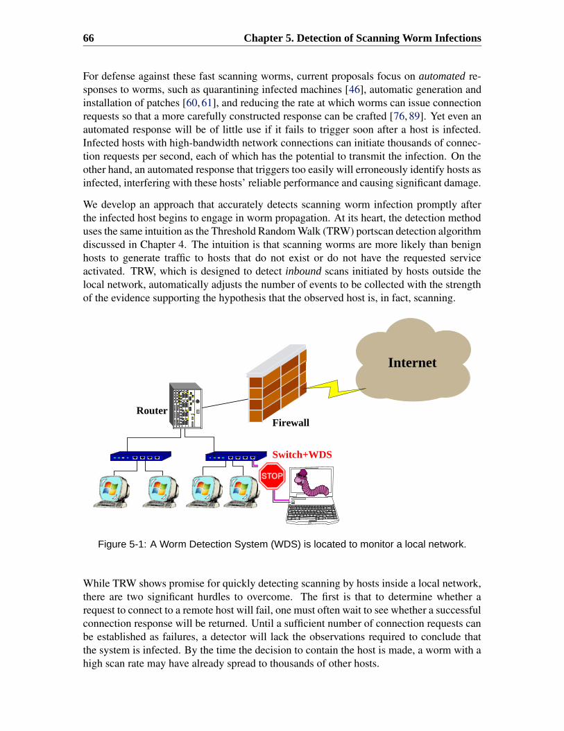
66 Chapter 5. Detection of Scanning Worm Infections
For defense against these fast scanning worms, current proposals focus on automated re-sponses to worms, such as quarantining infected machines [46], automatic generation andinstallation of patches [60, 61], and reducing the rate at which worms can issue connectionrequests so that a more carefully constructed response can be crafted [76, 89]. Yet even anautomated response will be of little use if it fails to trigger soon after a host is infected.Infected hosts with high-bandwidth network connections can initiate thousands of connec-tion requests per second, each of which has the potential to transmit the infection. On theother hand, an automated response that triggers too easily will erroneously identify hosts asinfected, interfering with these hosts’ reliable performance and causing significant damage.
We develop an approach that accurately detects scanning worm infection promptly afterthe infected host begins to engage in worm propagation. At its heart, the detection methoduses the same intuition as the Threshold Random Walk (TRW) portscan detection algorithmdiscussed in Chapter 4. The intuition is that scanning worms are more likely than benignhosts to generate traffic to hosts that do not exist or do not have the requested serviceactivated. TRW, which is designed to detect inbound scans initiated by hosts outside thelocal network, automatically adjusts the number of events to be collected with the strengthof the evidence supporting the hypothesis that the observed host is, in fact, scanning.
FirewallRouter
Switch+WDS
Internet
1 0
Figure 5-1: A Worm Detection System (WDS) is located to monitor a local network.
While TRW shows promise for quickly detecting scanning by hosts inside a local network,there are two significant hurdles to overcome. The first is that to determine whether arequest to connect to a remote host will fail, one must often wait to see whether a successfulconnection response will be returned. Until a sufficient number of connection requests canbe established as failures, a detector will lack the observations required to conclude thatthe system is infected. By the time the decision to contain the host is made, a worm with ahigh scan rate may have already spread to thousands of other hosts.

67
The second hurdle is that an observed host can change its behavior at any moment. TRWuses a single sequential hypothesis test per host and does not re-evaluate benign hosts overtime. Unlike an intrusion detection system observing remote hosts, a worm detector islikely to observe benign traffic originating from an infected host before it is infected. It istherefore necessary to adapt this method to continuously monitor hosts for indications ofscanning.
Figure 5-1 illustrates a network layout where one can set up a Worm Detection System(WDS), which monitors traffic generated from local hosts and automatically contains in-fected hosts to prevent further infection spread to other subnets within the local network.To detect infected hosts, the WDS need only process a small fraction of network events:a subset of connection request observations that we call first-contact connection requestsand the responses to these requests that complete the connections. A first-contact connec-tion request is a packet (TCP or UDP) addressed to a host with which the sender has notrecently communicated.1 These events are monitored because scans are mostly composedof first-contact connection requests.
In this work, we focus on detecting local hosts infected by a scanning worm, which searchesthrough the IP address space for new victims. Hence, our approach is not likely to detecttargeting worms that utilize other information about potentially vulnerable hosts. Examplesof targeting worms are topological worms (e.g., Morris), flash worms, and meta-serverworms (e.g., Santy).
In Section 5.1, we introduce a scan detection algorithm that we call a reverse sequentialhypothesis test (←−−HT ), and show how it can reduce the number of first-contact connectionsthat must be observed to detect scanning.2 This last-in, first-out event processing ensuresthat the number of observations ←−−HT requires to detect hosts’ scanning behavior is notaffected by the presence of benign network activity that may be observed before scanningbegins.
In Section 5.2, we present a credit-based algorithm for limiting the rate at which a host mayissue the first-contact connections that are indicative of scanning activity. This credit-basedconnection rate limiting (CBCRL) algorithm results in significantly fewer false positives(unnecessary rate limiting) than existing approaches.
When combined, this two-pronged approach is effective because these two algorithms arecomplementary. Without credit-based connection rate limiting, a worm could rapidly issuethousands of connection requests before enough connection failures have been observed by←−−HT so that it can report the worm’s presence. Because ←−−HT processes connection successand failure events in the order that connection requests are issued, false alarms are lesslikely to occur than if we used an approach purely relying on credit-based connection rate
1This definition of the first-contact connection request can be extended to differentiate servers runningon a same host by taking a destination port into account. For example, two connection requests to a samedestination host can be both first-contact connection requests by the extended definition if one goes to port80 (Web server) and the other to port 25 (mail server).
2The letters in this abbreviation, ←−−HT , stand for Hypothesis Testing and the arrow indicates the reversesequential order in which observations are processed.

68 Chapter 5. Detection of Scanning Worm Infections
limiting, for which first-contact connections attempts are assumed to fail until the evidenceproves otherwise.We demonstrate the utility of these combined algorithms with the trace-driven simulationsdescribed in Section 5.3. The results of the simulations are presented in Section 5.4. Thelimitations of our approach, including strategies that worms could attempt to avoid de-tection, are presented in Section 5.5. We conclude with a discussion of future work inSection 5.6.
5.1 Reverse Sequential Hypothesis TestingIn this section, we present an on-line algorithm for detecting the presence of scannerswithin a local network by observing a host’s network traffic. Here a scanner means ahost sending out packets or connection initiation requests to a set of arbitrarily pickeddestination IP addresses on a given destination port. We use a sequential hypothesis testfor its ability to adapt the number of observations required to make a decision to match thestrength of the evidence it is presented with.As with previous approaches to scan detection discussed in Chapter 4 and [55], we relyon the observation that only a small fraction of external addresses are likely to respond toa connection request at any given port. Benign hosts, which only contact systems whenthey have reason to believe that this connection request will be accepted, are more likely toreceive a response to a connection request.
Recall that a first-contact connection request is a packet (TCP or UDP) addressed to a hostwith which the sender has not communicated for a given period of time. When a localhost l initiates a first-contact connection request to a destination address, d, we classify theoutcome as either a “success” or a “failure”. If the request was a TCP SYN packet, theconnection is said to succeed if a SYN-ACK is received from d before a timeout expires. Ifthe request is a UDP packet, any UDP packet from d received before the timeout will do.We let Yi be a random (indicator) variable that represents the outcome of the ith first-contactconnection request by l, where
Yi =
{
0 if the connection succeeds1 if the connection fails
As defined in Chapter 2.1, we call H1 the hypothesis that host l is engaged in scanning(indicating infection by a worm) and H0 the null hypothesis that the host is not scanning.Here l is a host in the local network, unlike in Chapter 4. We assume that, conditional onthe hypothesis Hj , the random variables Yi|Hj i = 1, 2, . . . are independent and identicallydistributed. We can express the distribution of the Bernoulli random variable Yi as:
Pr[Yi = 0|H0] = θ0, Pr[Yi = 1|H0] = 1− θ0
Pr[Yi = 0|H1] = θ1, Pr[Yi = 1|H1] = 1− θ1
Given that connections originating at benign hosts are more likely to succeed than thoseinitiated by a scanner, θ0 > θ1.

5.1. Reverse Sequential Hypothesis Testing 69
Sequential hypothesis testing chooses between two hypotheses by comparing the likeli-hoods that the model would generate the observed sequence of events, Yn ≡ (Y1, . . . , Yn),under each hypothesis. It does this by maintaining the ratio Λ(Yn), the numerator of whichis the likelihood that the model would generate the sequence of events Yn under hypothesisH1, and the denominator under hypothesis H0.
Λ(Yn) ≡ Pr[Yn|H1]
Pr[Yn|H0](5.1)
We can write the change to Λ(Yn) as a result of the ithobservation as φ(Yi):
φ(Yi) ≡Pr[Yi|H1]
Pr[Yi|H0]=
θ1
θ0
if Yi = 0 (success)
1−θ1
1−θ0
if Yi = 1 (failure)(5.2)
This formula and the i.i.d. assumption enable us to rewrite Λ(Yn) inductively, such thatΛ(Y0) = 1, and Λ(Yn) may be calculated iteratively as each observation arrives.
Λ(Yn) =n∏
i=1
φ(Yi) = Λ(Yn−1)φ(Yn) (5.3)
One compares the likelihood ratio Λ(Yn) to an upper threshold, η1, above which we accepthypothesis H1, and a lower threshold, η0, below which we accept hypothesis H0. If η0 <Λ(Yn) < η1 then the result will remain inconclusive until more events in the sequence canbe evaluated.3 This is illustrated in Figure 5-2.
Y2 Y4Y3 Y5Y1
η1
η0
10 1 0 10
Figure 5-2: A log scale graph of Λ(Y) as each observation, Yi, is added to the sequence.Each success (0) observation decreases Λ(Y), moving it closer to the benign conclusionthreshold η0, whereas each failure (1) observation increases Λ(Y), moving it closer to theinfection conclusion threshold η1.
3Section 2.2 discusses how to set the thresholds in terms of a target false positive probability (α) and atarget detection probability (β).

70 Chapter 5. Detection of Scanning Worm Infections
5.1.1 Detecting Infection Events
In TRW, we assumed that each remote host was either a scanner or benign for the durationof the observed period. When a host was determined to be benign it would no longerbe observed. In contrast, in this work we are concerned with detecting infection events,in which a local host transitions from a benign state to an infected state. Should a hostbecome infected while a hypothesis test is already running, the set of outcomes observedby the sequential hypothesis test may include those from both the benign and infectedstates, as shown in Figure 5-3. Even if we continue to observe the host and start a newhypothesis test each time a benign conclusion is reached, the test may take longer thannecessary to conclude that an infection has occurred.
Yi Yi+1 Yi+4 Yi+5 Yi+6 Yi+7Yi+3Yi+2Yi−1i−2Y
10η
η10
0infection 1
11 1 1 101
Figure 5-3: A log scale graph tracing the value of Λ(Y) as it is updated for a series ofobservations that includes first-contact connection requests before (Yi−1 and Yi−2) andafter (Yi and beyond) the host was infected.
The solution to this problem is to run a new sequential hypothesis test as each connec-tion outcome is observed, evaluating these outcomes in reverse chronological order, asillustrated in Figure 5-4. To detect a host that was infected before it issued first-contactconnection i (event Yi), but after it had issued first-contact connection i − 1, a reverse se-quential hypothesis test (←−−HT ) would require the same number of observations to detect theinfection as would a forward sequential hypothesis that had started observing the sequenceat observation i. Because the most recent observations are processed first, the reverse testwill terminate before reaching the observations that were collected before infection.
Yi−1i−2Y Yi+5Yi+4Yi+3Yi+2Yi+1Yi
η1
10η
infection 10 0 1 11 01
Figure 5-4: A log scale graph tracing the value of Λ(Yi+5, Yi+4, . . .), in which the observa-tions in Y are processed in reverse sequential order. The most recent (rightmost) observa-tion is the first one processed.

5.1. Reverse Sequential Hypothesis Testing 71
When we used the sequential hypothesis testing in Chapter 4 to detect scanning of a localnetwork by remote hosts, the intrusion detection system could know a priori whether aconnection would fail given its knowledge of the network topology and services. Thus, theoutcome of a connection request from host i could immediately be classified as a successor failure observation (Yi) and Λ(Yn) could be evaluated without delay.
When a local host initiates first-contact connection requests to remote hosts, such as thoseshown in Figure 5-5, the worm detection system cannot immediately determine if the con-nection will succeed or fail. While some connection failures will result in a TCP RSTpacket or an ICMP packet [10], empirical evidence has shown that most do not [9]. Theremaining connection attempts can be classified as failures only after a timeout expires.
r2src:
Y1 = 1
Y5 = 1
Y4 = 1Y3 = 1
Y2 = 0
r5
r4dst:r3dst:r2dst:r1dst:
time time
timeout
WDSlocal host
dst:
Figure 5-5: The success of first-contact connection requests by a local host to remotehosts cannot be established by the Worm Detection System (WDS) until a response isobserved or a timeout expires.
While a sequential hypothesis test waits for unsuccessful connections to time out, a wormmay send thousands of additional connection requests with which to infect other systems.To limit the number of outgoing first-contact connections, a sequential hypothesis testingapproach must be paired with a method that limits connection initiation rates: the credit-based connection rate limiter described in Section 5.2 is one such scheme.
5.1.2 Optimizing the Computation of Repeated Reverse Sequential Hy-pothesis Tests
A straightforward implementation of the reverse sequential hypothesis testing requires thatan arbitrarily large sequence of first-contact connection observations be stored. An iterative

72 Chapter 5. Detection of Scanning Worm Infections
computation of the likelihood ratio, Equation (5.3) does not apply for a reverse sequentialhypothesis test. Instead, one has to maintain a sequence of observations from the beginningand step through a portion of this sequence each time a new observation is received in orderto run a new test starting at that observation. The computational resources required for thisimplementation may be onerous.
In this section, we show that there exists an iterative function for reverse sequential hypoth-esis tests:
Λ(Yn) = max(
1, Λ(Yn−1)φ(Yn))
Λ(Y0) ≡ 1
with state variable Λ(Yn), that can be calculated in the sequence in which events are ob-served, and that has the property that its value will exceed η1 if and only if a reverse se-quential hypothesis test would conclude from this sequence that the host was infected. φ isthe likelihood ratio of an individual event as defined in Equation (5.2).
We first prove the following lemma stating that if a reverse sequential hypothesis test re-ports an infection, our optimized function will also report an infection.
Lemma 1. For η1 > 1 and for mutually independent random variables Yi,
∀m ∈ [1, n] : Λ(Yn, Yn−1, . . . , Ym) ≥ η1 ⇒ Λ(Yn) ≥ η1 (5.4)
Proof. We begin by replacing Λ with its equivalent expression in terms of φ:
η1 ≤ Λ(Yn, Yn−1, . . . , Ym) =n∏
i=m
φ(Yi) (5.5)
We can place a lower bound on the value of Λ(Yn) by exploiting the fact that, in anyiteration, Λ cannot return a value less than 1.
Λ(Yn) = Λ(Y1, Y2, . . . , Yn)
≥ 1 · Λ(Ym, Ym+1, . . . , Yn)
≥n∏
i=m
φ(Yi)
≥ η1 (using Equation (5.5))
Thus, Λ(Yn, Yn−1, . . . , Ym) ≥ η1 ⇒ Λ(Yn) ≥ η1.
We must also prove that our optimized function will only report an infection when a reversesequential hypothesis test would also report an infection. Recall that a reverse sequentialhypothesis test will only report an infection if Λ exceeds η1 before falling below η0.
Lemma 2. For thresholds η0 < 1 < η1 and for mutually independent random variablesYi, if Λ(Yi) ≥ η1 for some i = n, but Λ(Yi) < η1 for all i ∈ [0, n − 1], then there exists asubsequence of observations starting at observation n and moving backward to observation

5.1. Reverse Sequential Hypothesis Testing 73
m ∈ [0, n − 1] for which Λ(Yn, Yn−1, . . . , Ym+1) ≥ η1 and such that there exists no k in[m + 1, n] such that Λ(Yn, Yn−1, . . . , Yk) ≤ η0.
Proof. Choose m as the largest observation index for which it held that:
Λ(Ym−1)φ(Ym) < 1
We know that m < n because Λ(Yn−1)φ(Yn) is greater than η1 which is in turn greater than1. Let m = 0 if the above relation does not hold for any observation with index greaterthan or equal to 1. It follows that Λ(Ym) = 1 and thus:
Λ(Ym+1) = φ(Ym+1)
Because we chose m such that Λ(Yj−1)φ(Yj) ≥ 1 for all j > m:
Λ(Yn) =n∏
j=m+1
φ(Yj)
= Λ(Yn, Yn−1, . . . , Ym+1)
Thus, Λ(Yn) ≥ η1 ⇒ Λ(Yn, Yn−1, . . . , Ym+1) ≥ η1.
To prove that there exists no k in [m + 1, n] such that Λ(Yn, Yn−1, . . . , Yk) ≤ η0, supposethat such a k exists. It follows that:
n∏
j=k
φ(Yj) ≤ η0 < 1 (5.6)
Recall that we chose m to ensure that:
η1 ≤n∏
j=m+1
φ(Yj) (5.7)
The product on the right hand side can be separated into factors from before and afterobservation k.
η1 ≤k−1∏
j=m+1
φ(Yj) ·n∏
j=k
φ(Yj)· (5.8)
We then use Equation (5.6) to substitute an upper bound of 1 on the latter product.
η1 <k−1∏
j=m+1
φ(Yj) ≤ Λ(Yk−1)
This contradicts the hypothesis that Λ(Yi) < η1 for all i ∈ [0, n− 1].
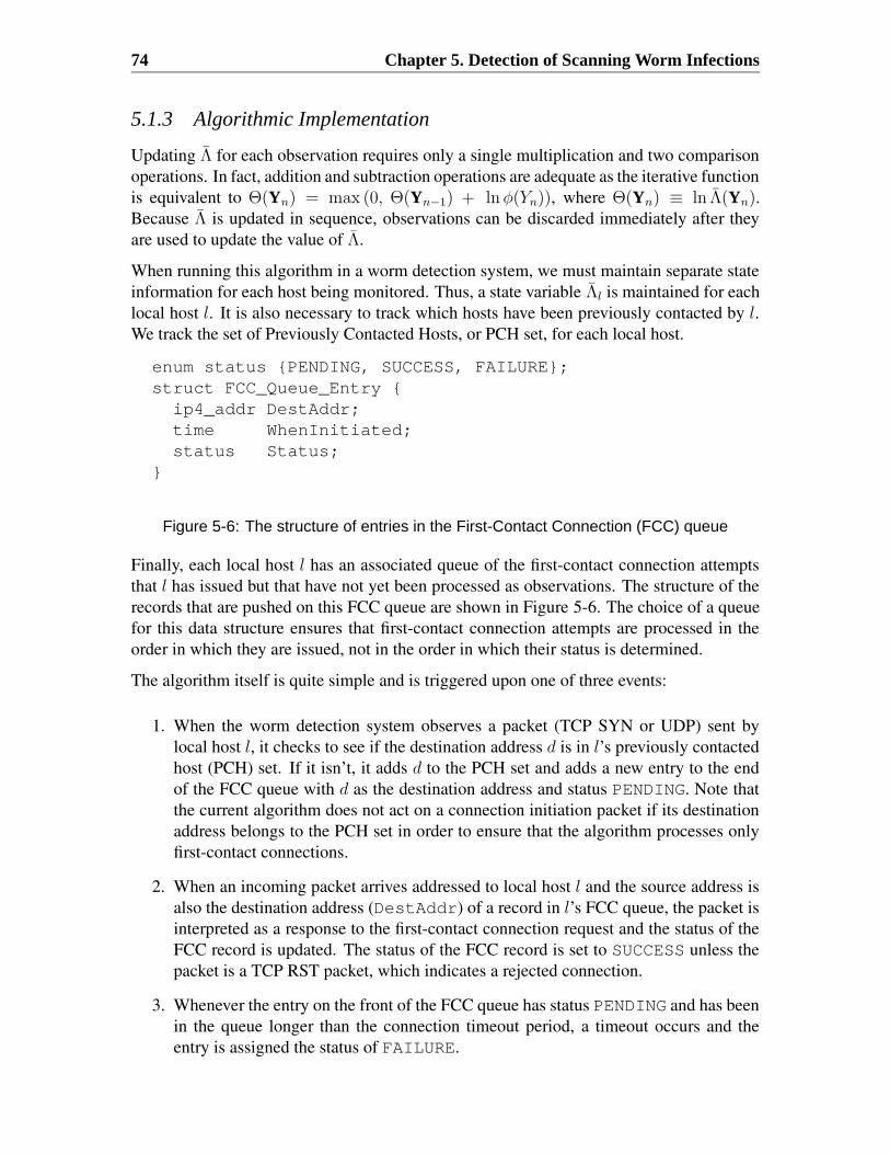
74 Chapter 5. Detection of Scanning Worm Infections
5.1.3 Algorithmic Implementation
Updating Λ for each observation requires only a single multiplication and two comparisonoperations. In fact, addition and subtraction operations are adequate as the iterative functionis equivalent to Θ(Yn) = max (0, Θ(Yn−1) + ln φ(Yn)), where Θ(Yn) ≡ ln Λ(Yn).Because Λ is updated in sequence, observations can be discarded immediately after theyare used to update the value of Λ.
When running this algorithm in a worm detection system, we must maintain separate stateinformation for each host being monitored. Thus, a state variable Λl is maintained for eachlocal host l. It is also necessary to track which hosts have been previously contacted by l.We track the set of Previously Contacted Hosts, or PCH set, for each local host.
enum status {PENDING, SUCCESS, FAILURE};struct FCC_Queue_Entry {ip4_addr DestAddr;time WhenInitiated;status Status;
}
Figure 5-6: The structure of entries in the First-Contact Connection (FCC) queue
Finally, each local host l has an associated queue of the first-contact connection attemptsthat l has issued but that have not yet been processed as observations. The structure of therecords that are pushed on this FCC queue are shown in Figure 5-6. The choice of a queuefor this data structure ensures that first-contact connection attempts are processed in theorder in which they are issued, not in the order in which their status is determined.
The algorithm itself is quite simple and is triggered upon one of three events:
1. When the worm detection system observes a packet (TCP SYN or UDP) sent bylocal host l, it checks to see if the destination address d is in l’s previously contactedhost (PCH) set. If it isn’t, it adds d to the PCH set and adds a new entry to the endof the FCC queue with d as the destination address and status PENDING. Note thatthe current algorithm does not act on a connection initiation packet if its destinationaddress belongs to the PCH set in order to ensure that the algorithm processes onlyfirst-contact connections.
2. When an incoming packet arrives addressed to local host l and the source address isalso the destination address (DestAddr) of a record in l’s FCC queue, the packet isinterpreted as a response to the first-contact connection request and the status of theFCC record is updated. The status of the FCC record is set to SUCCESS unless thepacket is a TCP RST packet, which indicates a rejected connection.
3. Whenever the entry on the front of the FCC queue has status PENDING and has beenin the queue longer than the connection timeout period, a timeout occurs and theentry is assigned the status of FAILURE.

5.2. Credit-Based Connection Rate Limiting 75
When any of the above events causes the entry at the front of the FCC queue to have statusother than PENDING, it is dequeued and Λl is updated and compared to η1. If Λl ≥ η1, wehalt testing for host l and immediately conclude that l is infected. Dequeuing continues solong as Λl < η1, the front entry of the FCC queue has status other than PENDING, and thequeue is not empty.
5.2 Credit-Based Connection Rate Limiting
It is necessary to limit the rate at which first-contact connections can be initiated in orderto ensure that worms cannot propagate rapidly between the moment scanning begins andthe time at which the scan’s first-contact connections have timed out and been observed byour reverse sequential hypothesis test (←−−HT ).
Twycross and Williamson [76, 89] use a technique they call a virus throttle to limit out-going first-contact connections. When observing a given host, their algorithm maintainsa working set of up to five hosts previously contacted by the host they are observing. Intheir work, a first-contact connection is a connection to a host that is not in this workingset. First-contact connections issued when the working set is full are not sent out, but in-stead added to a queue. Once per second, the least recently used entry in the working set isremoved and, if the pending queue of first-contact connection requests is not empty, a re-quest is pulled off the queue, delivered, and its destination address is added to the workingset. All requests in the queue with the same destination address are also removed from thequeue and delivered.
Virus throttling is likely to interfere with HTTP connection requests for embedded objects,as many Web pages contain several or more embedded objects each of which may be lo-cated on a distinct server. While a slow but bursty stream of requests from a Web browserwill eventually be released by the throttle, mail servers, Web crawlers, and other legitimateservices that issue first-contact connections at a rate greater than once per second will over-flow the queue. In this case, the virus throttling algorithm quarantines the host and allowsno further first-contact connections.
To achieve rate limiting with a better false positive rate we once again present a solutioninspired by sequential hypothesis testing and that relies on the observation that benign first-contact connections are likely to succeed whereas those issued by scanners are likely to fail.This credit-based approach, however, is unlike←−−HT in that it assumes that a connection willfail until evidence proves otherwise. Because it does not wait for a timeouts to act, it canreact immediately to a burst of connections and halt the flow so that ←−−HT can then make amore informed decision as to whether the host is infected. As it does not force connectionsto be evaluated in order, CBCRL can also immediately process evidence of connectionsuccesses. This will enable it to quickly increase the allowed first-contact connection ratewhen these requests are benign.
CBCRL, as summarized in Table 5.1, works by allocating to each local host, l, a start-ing balance of C0 credits, which can be used for issuing first-contact connection requests.Whenever a first-contact connection request is observed, the sending host’s balance is

76 Chapter 5. Detection of Scanning Worm Infections
decremented by p. If the successful acknowledgment of a first-contact connection is ob-served, the host that initiated the request is issued with q additional credits. No action istaken when connections fail, as the cost of issuing a first-contact connection has alreadybeen deducted from the issuing host’s balance. Finally, first-contact connection requestsare blocked if the host does not have any credit available (Cl = 0).
Table 5.1: The underlying equations behind credit-based connection rate limiting. Changesto a host’s balance are triggered by the first-contact connections (FCCs) it initiates and bythe passing of time.
Event Change to Cl
Starting balance Cl ← C0
FCC issued by l Cl ← Cl − pFCC succeeds Cl ← Cl + q (q > p)Every second Cl ← max(C0, rCl) if Cl > C0 (0 < r < 1)Allowance Cl ← 1 if Cl = 0 for t seconds
If a first-contact connection succeeds with probability θ, its expected payoff from issuingthat connection is its expected success credit minus its cost, or qθ−p. This payoff is positivefor θ > p
qand negative otherwise. To penalize a host with a less than 50% success rate,
we set q = 2 and p = 1. Hosts that scan with a low rate of successful connections (< p
q)
will quickly consume their credits whereas benign hosts that issue first-contact connectionswith high rates of success will increase their credits each time they invest them.
As described so far, the algorithm could result in two undesirable states. First, a host couldacquire a large number of credits while performing a benign activity (e.g., Web crawling)which could be used later by a scanning worm. Second, a network outage could cause abenign host to use all of its credits after which it would starve for a lack of first-contactconnection successes.
These problems are addressed by providing each host with a small allowance and by puttingin place a high rate of inflation. If a host has been without credits for t seconds, we issuethe host a single credit (Cl ← 1 if Cl ≤ 0). This not only ensures that the host does notstarve, but enables us to collect another observation to feed into the hypothesis test (←−−HT ).
Because←−−HT , as configured below in Section 5.3, observes all first-contact connection re-quests as successes or failures within three seconds, providing a starving process with acredit allowance only after more than three seconds have passed ensures that←−−HT will havebeen executed on all previously issued first-contact connection requests. In other words, t
should be set such that it is greater than a timeout value based on which ←−−HT determines afailure for a non-responding first-contact connection request. If←−−HT has already concludedthat the host is a worm, it is expected that the system will be quarantined and so no requestswill reach their destination regardless of the credit balance.
For each second that passes, a host that has acquired more than C0 credits will be forcedto surrender up to (1− r) of them, but not so many as to take its balance below C0 (Cl ←

5.3. Experimental Setup 77
max(C0, rCl) if Cl > C0). A host that is subject to the maximum inflation rate, with afirst-contact connection rate γ, success rate θ > 0, and credit balance Cl,t at time t, will seethis balance reach an equilibrium state C when C = Cl,t = Cl,t+1.
Cl,t+1 = r[Cl,t + γ · (qθ − p)]
C = r[C + γ · (qθ − p)]
C =r
1− r· γ · (qθ − p)
One way to choose the inflation constant r is to ensure that, in the upcoming second, a hostthat has a perfect first-contact connection success rate (θ = 1) will have twice as manycredits as it could have needed in the previous second. In the case of p = 1 and q = 2:
r
1− r· γ = 2 · γ
r =2
3
Also note that the maximum inflation rate, which seems quite steep, is only fully appliedwhen C ≥ 15, which in turn occurs only when the first-contact connection rate r is greaterthan 7.5 requests per second. Twycross and Williamson’s virus throttle, on the other hand,can only assume that any host with a first-contact connection rate consistently greater than1 per second is a worm.
The constant of 10 was chosen for the starting credit balance (and for the equilibriumminimum credit balance for benign hosts with first-contact connection rates below 5 re-quests/second) in order to match the requirements of our sequential hypothesis test (←−−HT )as currently configured (see parameters in Section 5.3), which itself requires a minimum of10 observations in order to conclude that a host is engaged in scanning. Slowing the rate atwhich the first 10 observations can be obtained will only delay the time required by←−−HT toconclude that a host is engaged in scanning. Should the parameters of←−−HT be reconfiguredand the minimum number of observations required to conclude a host is a scanner change,the starting credit balance for rate-limiting can be changed to match it.
5.3 Experimental SetupWe evaluated our algorithms using two traces collected at the peering link of a mediumsized ISP: one collected in April 2003 (isp-03) containing 404 active hosts and the otherin January 2004 (isp-04) containing 451 active hosts. These traces, summarized in Ta-ble 5.2, were collected using tcpdump.
Obtaining usable traces was difficult. Due to privacy concerns, network administrators areloathe to share any traces, let alone those that contain payload data in addition to headers.Yet we required the payload data in order to manually determine which, if any, worm waspresent on a host that was flagged as infected.

78 Chapter 5. Detection of Scanning Worm Infections
Table 5.2: Summary of network tracesisp-03 isp-04
Date 2003/04/10 2004/01/28Duration 627 minutes 66 minutes
Total outbound connection attempts 1,402,178 178,518Total active local host 404 451
In configuring the reverse sequential hypothesis test (←−−HT ), first-contact connection requestswere interpreted as failures if they were not acknowledged within a three second grace pe-riod. First-contact connection requests for which TCP RST packets were received in re-sponse were immediately reported as failure observations. Connection success probabilityestimates were chosen to be:
θ0 = 0.7 θ1 = 0.1
Confidence requirements were set to:
α = 0.00005 β = 0.99
Note that these confidence requirements are for each reverse sequential hypothesis test, andthat a test is performed for each first-contact connection that is observed. Therefore, thefalse positive rate (α) is chosen to be particularly low as testing will occur many times foreach host.For each local host we maintained a Previously Contacted Host (PCH) set of only the last64 destination addresses that each local host had communicated with (LRU replacement).In the experiment, a first-contact connection request was any TCP SYN packet or UDPpacket addressed to a host that was not in the local host’s PCH set. While using a fixedsized PCH set demonstrates the efficacy of our test under the memory constraints that arelikely to occur when observing large (e.g., class B) networks, this fixed memory usagecomes at a cost. As described in Section 5.5, it is possible for a worm to exploit limitationsin the PCH set size to avoid having its scans detected.For comparison, we also implemented Twycross and Williamson’s virus throttle as de-scribed in [76]. Because our traces contain only those packets seen at the peering point,our results may differ from a virus throttle implemented at each local host as Twycross andWilliamson recommend. However, because observing connections farther from the hostresults in a reduction in the number of connections observed, it should only act to reducethe reported number of false positives in which benign behavior is throttled.All algorithms were implemented in Perl. We used traces that had been pre-processed bythe Bro Network Intrusion Detection System [1, 52].We did not process FTP data-transfer, finger, and ident connections as these connectionsare the result of local hosts responding to remote hosts, and are not likely to be acceptedby a host that has not issued a request for such a connection. These connections are thusunlikely to be useful for worm propagation.

5.4. Results 79
5.4 Results←−−HT detected two hosts infected with Code Red II [13, 69] from the April, 2003 trace(isp-03). Our test detected one host infected with Blaster [24], three hosts infected withMyDoom [26, 85], and one host infected with Mimail.j [25] from the January, 2004 trace(isp-04). The worms were conclusively identified by painstakingly comparing the loggedtraffic with the cited worm descriptions at various online virus/worm information libraries.Our test also identified four additional hosts that we classify as HTTP scanners becauseeach sent SYN packets to port 80 of at least 290 addresses within a single class B network.These results are summarized in Table 5.3.
Table 5.3: Alarms reported by reverse sequential hypothesis testing combined with credit-based rate limiting. The cause of each alarm was later identified manually by comparingobserved traffic to signature behaviors described at online virus libraries.
isp-03 isp-04Worms/Scanners detected
Code Red II 2 0Blaster 0 1MyDoom 0 3
Mimail.j 0 1HTTP (other) 3 1
Total 5 6False alarms
HTTP 0 3SMTP 0 3
Total 0 6P2P detected 6 11Total identified 11 23
While peer-to-peer applications are not necessarily malicious, many network administra-tors do not classify them as benign. Peer-to-peer file sharing applications also exhibitambiguous network behavior, as they attempt to contact a large number of transient peersthat are often unwilling or unavailable to respond to connection requests. While peer-to-peer clients are deemed undesirable on most of the corporate networks that we envision ourapproach being used to protect, it would be unfair to classify these hosts as infected. Forthis reason we place hosts that we detect running peer-to-peer applications into their owncategory. Networks that allow peer-to-peer traffic may avoid these false alarms by limitingthe detection algorithm to outgoing traffic to the well known port numbers [75]. However,this may not eliminate false alarms due to peer-to-peer applications because some of themtunnel through port 80.
Three additional false alarms were reported for three of the 60 (isp-04) total hosts trans-mitting SMTP traffic. We suspect the false alarms are the result of bulk retransmission ofthose emails that have previously failed when the recipients’ mail servers were unreachable.
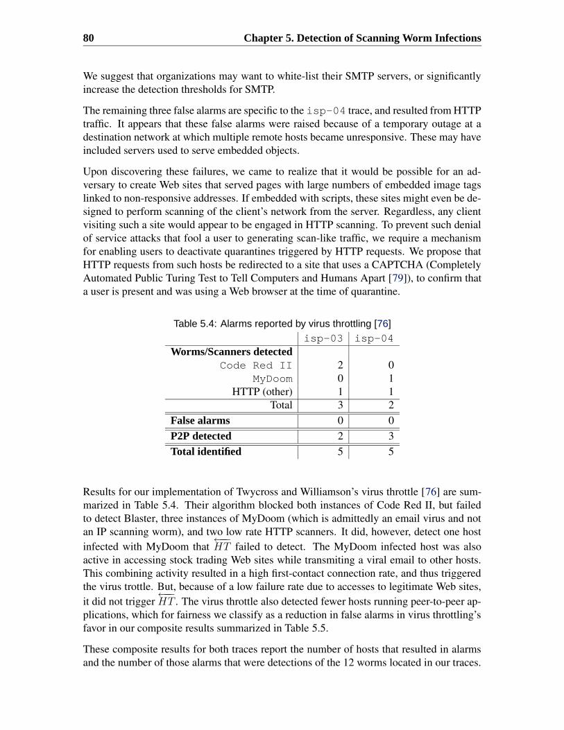
80 Chapter 5. Detection of Scanning Worm Infections
We suggest that organizations may want to white-list their SMTP servers, or significantlyincrease the detection thresholds for SMTP.
The remaining three false alarms are specific to the isp-04 trace, and resulted from HTTPtraffic. It appears that these false alarms were raised because of a temporary outage at adestination network at which multiple remote hosts became unresponsive. These may haveincluded servers used to serve embedded objects.
Upon discovering these failures, we came to realize that it would be possible for an ad-versary to create Web sites that served pages with large numbers of embedded image tagslinked to non-responsive addresses. If embedded with scripts, these sites might even be de-signed to perform scanning of the client’s network from the server. Regardless, any clientvisiting such a site would appear to be engaged in HTTP scanning. To prevent such denialof service attacks that fool a user to generating scan-like traffic, we require a mechanismfor enabling users to deactivate quarantines triggered by HTTP requests. We propose thatHTTP requests from such hosts be redirected to a site that uses a CAPTCHA (CompletelyAutomated Public Turing Test to Tell Computers and Humans Apart [79]), to confirm thata user is present and was using a Web browser at the time of quarantine.
Table 5.4: Alarms reported by virus throttling [76]isp-03 isp-04
Worms/Scanners detectedCode Red II 2 0
MyDoom 0 1HTTP (other) 1 1
Total 3 2False alarms 0 0P2P detected 2 3Total identified 5 5
Results for our implementation of Twycross and Williamson’s virus throttle [76] are sum-marized in Table 5.4. Their algorithm blocked both instances of Code Red II, but failedto detect Blaster, three instances of MyDoom (which is admittedly an email virus and notan IP scanning worm), and two low rate HTTP scanners. It did, however, detect one hostinfected with MyDoom that ←−−HT failed to detect. The MyDoom infected host was alsoactive in accessing stock trading Web sites while transmiting a viral email to other hosts.This combining activity resulted in a high first-contact connection rate, and thus triggeredthe virus trottle. But, because of a low failure rate due to accesses to legitimate Web sites,it did not trigger←−−HT . The virus throttle also detected fewer hosts running peer-to-peer ap-plications, which for fairness we classify as a reduction in false alarms in virus throttling’sfavor in our composite results summarized in Table 5.5.
These composite results for both traces report the number of hosts that resulted in alarmsand the number of those alarms that were detections of the 12 worms located in our traces.

5.4. Results 81
Table 5.5: Composite results for both traces: A total of 7 HTTP scanning worms and 5email worms were present.
Alarms Detection Efficiency Effectiveness←−−HT 34 11 0.324 0.917virus-throttling 10 5 0.500 0.417
We also include the efficiency, which is the number of detections over the total number ofalarms, and the effectiveness, which is the total number of detections over the total numberof infected hosts we have found in these traces. While←−−HT is somewhat less efficient thanvirus throttling, we believe that the more-than-two-fold increase in effectiveness is wellworth the trade-off. In addition, corporate networks that forbid peer-to-peer file sharingapplications will see a two-fold increase in efficiency.
Table 5.6 shows the number of hosts that had connection requests blocked by the CBCRLalgorithm and the number of hosts that were rate-limited by Twycross and Williamson’salgorithm. For credit-based connection rate limiting, we say that a machine has been ratelimited if a single packet is dropped. For the virus throttle, we say that a machine has beenrate limited if the outgoing delay queue length is greater than five, giving Twycross andWilliamson the benefit of the doubt that users won’t notice unless connections are severelythrottled. CBCRL only limited the rates of hosts that our reverse sequential hypothesis testreported as infected. In contrast, even given our generous definition, more than 10% of thehosts in both traces were rate limited by Twycross and Williamson’s algorithm.
Table 5.6: Comparison of rate limiting by CBCRL vs. virus throttlingCBCRL Virus Throttling
isp-03 isp-04 isp-03 isp-04Worms/Scanners 5 1 3 4
P2P 4 8 3 7Unnecessary rate limiting 0 0 84 59
Table 5.7 reports the number of first-contact connections permitted by the two approachesfor those scanners that both detected. Code Red II is a fast scanner, and so virus throttlingexcels in blocking it after 6 to 7 connection requests. This speed is expected to come atthe price of detecting any service, malicious or benign, that issues high-rate first-contactconnections.←−−HT with credit-based connection rate limiting detects worms after a somewhat higher num-ber of first-contact connections are permitted (10), but does so regardless of the scanningrate. Whereas our approach detects a slow HTTP scanner after 10 first-contact connectionrequests, the virus throttle requires as many as 526.

82 Chapter 5. Detection of Scanning Worm Infections
Table 5.7: The number of first-contact connections permitted before hosts were reported asinfected: the value pairs represent individual results for two different Code Red II infectionsand two different HTTP scanners. ←−−
HT with CBCRL Virus ThrottlingCode Red II 10,10 6,7
Other HTTP scanners 10,10 102,526
5.5 LimitationsCBCRL is resilient to network uplink outages as hosts starved for credits will receive anallowance credit seconds after the network is repaired. Unfortunately, this will be of littleconsolation as Reverse Sequential Hypothesis Testing (←−−HT ) may have already concludedthat all hosts are scanners. This may not be a problem if network administrators are giventhe power to invalidate observations made during the outage period, and to automaticallyreverse any quarantining decisions that would not have been taken without these invalidobservations.
Of greater concern is that both ←−−HT and CBCRL rely exclusively on the observation thathosts engaged in scanning will have lower first-contact connection success rates than be-nign hosts. New hypotheses and tests are required to detect worms for which this statisticalrelationship does not hold.
Also problematic is that two instances of a worm on different networks could collaborate toensure that none of their first-contact connections will appear to fail. For example, if wormA does not receive a response to a first-contact connection request after half the timeoutperiod, it could send a message to worm B asking it to forge a connection response. Thisforged response attack prevents our system from detecting connection failures. To thwartthis attack for TCP connections, a worm detection system implemented on a router canmodify the TCP sequence numbers of traffic as it enters and leaves the network. For ex-ample, the result of a hash function h(IPlocal, IPremote, salt) may be added to all sequencenumbers on outgoing traffic and subtracted from all incoming sequence numbers. The useof the secret salt prevents the infected hosts from calculating the sequence number usedto respond to a connection request which they have sent, but not received. By storing thecorrect sequence number in the FCC queue, responses can then be validated by the wormdetection system. However, modifying sequence numbers can disrupt a pre-existing con-nection that is already in progress when the detection system starts running. It is importantthat the detection system modifies a packet’s sequence number (or acknowledgement num-ber) only if the packet belongs to a connection that is initiated by a local host and theconnection’s initial SYN packet has been observed by the detection system.
Another concern is the possibility that a worm could arrive at its target already in possessionof a list of known repliers – hosts that are known to reply to connection requests at a givenport. This known-replier attack could employ lists that are programmed into the worm atcreation, or accumulated by the worm as it spreads through the network. First-contact con-nections to these known-repliers will be very likely to succeed and can be interleaved with

5.6. Summary 83
scans to raise the first-contact connection success rate. A one to one interleaving is likelyto ensure that more than half of all connections succeed. This success rate would enablethe scanner to bypass credit-based connection rate limiting, and delay detection by ReverseSequential Hypothesis Testing until the scanner had contacted all of its known-repliers.What’s worse, a worm could avoid detection altogether if the detection system defines afirst-contact connection with respect to a fixed sized previously contact host (PCH) set.If the PCH set tracks only the n previously visited hosts, the scanner can cycle through(n/2)+1 known-repliers, interleaved with as many new addresses, and never be detected.4
To prevent a worm from scanning your local network by interleaving connections to known-repliers outside of your network, Weaver et al. [83] propose that one hypothesis test be runfor local connections (i.e., those within the same IP block) and another for connections toremote hosts. If hosts in your local network are widely and randomly dispersed through alarge IP space,5 then a worm will have a low probability of finding another host to infectbefore being quarantined.
A worm might also avoid detection by interleaving scanning with other apparently benignbehavior, such as Web crawling. A subset of these benign interleaving attacks can beprevented by detecting scanners based on the destination port they target in addition to thesource IP of the local host. While it is still fairly easy to create benign looking traffic forports such as HTTP, for which one connection can lead to information about other activehosts receptive to new connections, this is not the case for ports such as those used by SSH.Running separate scan detection tests for each destination port that a local host addressescan ensure that connections to one service aren’t used to mask scans to other services.
Finally, if an infected host can impersonate other hosts, the host could escape quarantineand cause other (benign) hosts to be quarantined. To address these address impersonationattacks, it is important that a complete system for network quarantining include strongmethods for preventing IP masquerading by its local hosts, such as switch-level egressfiltering. Host quarantining should also be enforced as close to the host as is possiblewithout relying on the host to quarantine itself. If these boundaries cannot be enforcedbetween each host, one must assume that when one machine is infected, all of the machineswithin the same boundary will also be infected.
5.6 Summary
When combined, credit-based connection rate limiting and reverse sequential hypothesistesting ensure that worms are quickly identified with an attractively low false alarm rate.While no current system can detect all possible worms, our new approach is a significantimprovement over prior methods, which detect a smaller range of scanners and unnec-essarily delay network traffic. What’s more, the techniques introduced in this work lendthemselves to efficient implementation, as they need only be activated to observe a small
4For detecting such a worm, a random replacement policy will be superior to an LRU replacement policy,but will still not be effective enough for long known-replier lists.
5Randomly dispersing local hosts through a large IP space can be achieved by using a network addresstranslation (NAT) switch.
84 Chapter 5. Detection of Scanning Worm Infections
subset of network events and require little calculation for the common case that traffic isbenign.
As worm authors become aware of the limitations discussed in Section 5.5, it will be nec-essary to revise our algorithms to detect scanning at the resolution of the local host (sourceaddress) and targeted service (destination port), rather than looking at the source host alone.Solutions for managing the added memory requirements imposed by this approach havebeen explored by Weaver, Staniford, and Paxson [83].
The intrusiveness of credit-based connection rate limiting, which currently drops outgoingconnection requests when credit balances reach zero, can be further reduced. Instead ofhalting outgoing TCP first-contact connection requests from hosts that do not maintain apositive credit balance, the requests can be sent immediately and the responses can be helduntil a positive credit balance is achieved. This improvement has the combined benefits ofreducing the delays caused by false rate limiting while simultaneously ensuring that fewerconnections are allowed to complete when a high-speed scanning worm issues a burst ofconnection requests. As a result, the remaining gap in response speed between credit-basedconnection rate limiting and Twycross and Williamson’s virus throttle can be closed whilefurther decreasing the risk of acting on false positives.
Finally, we can employ additional indicators of infection to further reduce the number offirst-contact connection observations required to detect a worm. For example, it is reason-able to conclude that, when a host is deemed to be infected, those hosts to which it has mostrecently initiated successful connections are themselves more likely to be infected (as wasthe premise behind GrIDS [68]). We propose that this be accomplished by adding an eventtype, the report of an infection of a host that has recently contacted the current host, to ourexisting hypothesis test.
Chapter 6
Detection of Targeting WormPropagations
The previous chapter presented algorithms for detecting network worms that use randomscanning to discover new victims. This chapter describes an algorithm for detecting fast-propagating worms that use high-quality targeting information. It then presents a unifiedframework for detecting network worms independently of their target discovery strategy.
If a network worm penetrates a site’s perimeter, it can quickly spread to other vulnera-ble hosts inside the site. The infection propagates by the compromised host repeatedlyattempting to contact and infect new potential victims. Figure 6-1 illustrates a situationwhere a worm bypasses a firewall and then propagates to local machines via an infectedlaptop plugged in to a local network. The traffic pattern of fast worm propagation—a singlehost quickly contacting many different hosts—is a prominent feature across a number oftypes of worms, and detecting such patterns constitutes the basis for several worm detectionapproaches [14, 76].
The problem of accurately detecting such worm propagation becomes particularly acutefor enterprise networks comprised of a variety of types of hosts running numerous, dif-ferent applications. This diversity makes it difficult to tune existing worm detection meth-ods [14,76] that presume preselected thresholds for connection rates and window sizes overwhich to compute whether a host’s activity is “suspicious.” First, finding a single thresholdrate that accommodates most of benign hosts requires excessive tuning because of diverseapplication behaviors (e.g., a Web browser generating multiple concurrent connections tofetch embedded objects vs. an SSH client connecting to a server). Second, the windowsize chosen to compute the average rate affects the detection speed and accuracy; if toosmall, the detection algorithm is less resilient to small legitimate connection bursts, but iftoo big, the detection algorithm reacts slowly to fast propagating worms, for which promptresponse is vital.
We first develop an algorithm for detecting fast-propagating worms that use high-qualitytargeting information. We base our approach on analyzing the rate at which hosts initi-ate connections to new destinations. One such class of worms are those that spread in a
85

86 Chapter 6. Detection of Targeting Worm Propagations
Switch
Router
Firewall
Internet
1 0
Figure 6-1: Worm propagation inside a site
topological fashion [67, 82]: they gather information on the locally infected host regard-ing other likely victims. For example, the Morris worm examined .rhosts files to see whatother machines were known to the local machine [20, 63]. A related technique is the useof meta-servers, such as worms that query search engines for likely victims [22]. Thesetargeting worms can spread extremely quickly, even using relatively low-rate scanning, be-cause the vulnerability density of the addresses they probe is so much higher than if theyuse random scanning. Furthermore, these worms can evade many existing worm defensesystems that rely on the artifacts of random scanning such as number of failed connectionsand the absence of preceding DNS lookups [14, 83, 84].
Our detection algorithm, Rate-Based Sequential Hypothesis Testing (RBS), operates ona per-host and per-connection basis and does not require access to packet contents. It isbuilt on a probabilistic model that captures benign network characteristics, which enablesus to discriminate between benign traffic and worm traffic. RBS also provides an analyticframework that enables a site to tailor its operation to its network traffic pattern and securitypolicies.
We then present RBS + TRW, a unified framework for detecting fast-propagating wormsindependent of their target discovery strategy. RBS + TRW is a blend of RBS and theThreshold Random Walk (TRW) algorithm from Chapter 4, which rapidly discriminatesbetween random scanners and legitimate traffic based on their differing rates of connectionfailures.
Section 6.1 presents an analysis of network traces we obtained from two internal routersof Lawrence Berkeley National Laboratory (LBL). Such data allow us to assess RBS’sefficacy in detecting worms that remain inside an organization network, rather than justthose that manifest in a site’s external Internet traffic (a limitation of previous studies).
6.1. Data Analysis 87
The traced traffic includes more than 650 internal hosts, about 10% of the total at thesite. We examine the distribution of the time between consecutive first-contact connectionrequests, defined in Chapter 5 as a packet addressed to a host with which the sender has notrecently communicated. Our analysis finds that for benign network traffic, these interarrivaltimes are bursty, but within the bursts can be approximately modeled using exponentialdistributions with a few hundred millisecond average intervals.
In Section 6.2, we develop the RBS algorithm, based on the same sequential hypothesistesting framework as TRW. RBS quickly identifies hosts that initiate first-contact connec-tion requests at a rate n times higher than that of a typical benign host. RBS updates itsdecision process upon each data arrival, triggering an alarm after having observed enoughempirical data to make a distinction between the candidate models of (somewhat slower)benign and (somewhat faster) malicious host activity.
In Section 6.3, we evaluate RBS using trace-driven simulations. We find that when n issmall, RBS requires more empirical data to arrive at a detection decision; for example,it requires on average 10.4 first-contact connections when n = 5. However, when n islarger, RBS provides accurate and fast detection. On the other hand, we show that a fixed-threshold rate-based scheme will inevitably require more difficult tradeoffs between falsepositives and false negatives.
Section 6.4 presents RBS + TRW, which automatically adapts between the rate at whicha host initiates first-contact connection requests and observations of the success of theseattempts, combining two different types of worm detection. Using datasets that containactive worms caught in action, we show that RBS + TRW provides fast detection of twohosts infected by Code Red II worms, while generating less than 1 false alarm per hour.
6.1 Data AnalysisWe hypothesize that we can bound a benign host’s network activity by a reasonably lowfan-out per unit time, where we define fan-out as the number of first-contact connectionrequests a given host initiates. This fan-out per unit time, or fan-out rate, is an importanttraffic measure that we hope will allow us to separate benign hosts from relatively slowlyscanning worms. In this section, we analyze traces of a site’s internal network traffic,finding that a benign host’s fan-out rate rarely exceeds a few first-contact connections persecond, and time intervals between those connections can be approximately modeled asexponentially distributed.
We analyze a set of 22 anonymized network traces, each comprised of 10 minutes’ of trafficrecorded at LBL on Oct. 4, 2004. These were traced using tcpdump at two internal routerswithin LBL, enabling them to collect bidirectional traffic originated by internal hosts toboth external hosts outside LBL and to other internal hosts inside LBL. While ideally wewould have such traces from a number of different sites in order to assess the range ofbehavior normally seen, such traces have to date been unavailable. Indeed, we believe theinternal traces to which we have access are unique or nearly so for the research communityat present. Thus, we view them as highly valuable, if fundamentally limited, though weneed to continually keep in mind the caution that we should not readily generalize from
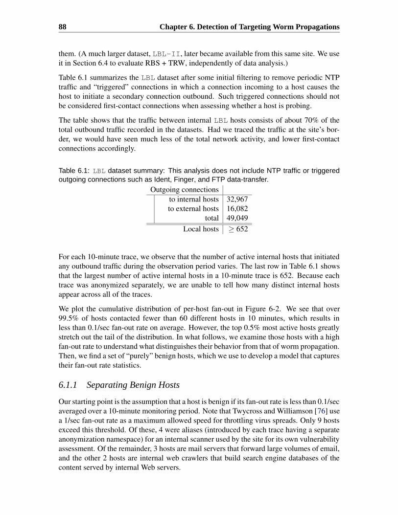
88 Chapter 6. Detection of Targeting Worm Propagations
them. (A much larger dataset, LBL-II, later became available from this same site. We useit in Section 6.4 to evaluate RBS + TRW, independently of data analysis.)
Table 6.1 summarizes the LBL dataset after some initial filtering to remove periodic NTPtraffic and “triggered” connections in which a connection incoming to a host causes thehost to initiate a secondary connection outbound. Such triggered connections should notbe considered first-contact connections when assessing whether a host is probing.
The table shows that the traffic between internal LBL hosts consists of about 70% of thetotal outbound traffic recorded in the datasets. Had we traced the traffic at the site’s bor-der, we would have seen much less of the total network activity, and lower first-contactconnections accordingly.
Table 6.1: LBL dataset summary: This analysis does not include NTP traffic or triggeredoutgoing connections such as Ident, Finger, and FTP data-transfer.
Outgoing connectionsto internal hosts 32,967to external hosts 16,082
total 49,049Local hosts ≥ 652
For each 10-minute trace, we observe that the number of active internal hosts that initiatedany outbound traffic during the observation period varies. The last row in Table 6.1 showsthat the largest number of active internal hosts in a 10-minute trace is 652. Because eachtrace was anonymized separately, we are unable to tell how many distinct internal hostsappear across all of the traces.
We plot the cumulative distribution of per-host fan-out in Figure 6-2. We see that over99.5% of hosts contacted fewer than 60 different hosts in 10 minutes, which results inless than 0.1/sec fan-out rate on average. However, the top 0.5% most active hosts greatlystretch out the tail of the distribution. In what follows, we examine those hosts with a highfan-out rate to understand what distinguishes their behavior from that of worm propagation.Then, we find a set of “purely” benign hosts, which we use to develop a model that capturestheir fan-out rate statistics.
6.1.1 Separating Benign Hosts
Our starting point is the assumption that a host is benign if its fan-out rate is less than 0.1/secaveraged over a 10-minute monitoring period. Note that Twycross and Williamson [76] usea 1/sec fan-out rate as a maximum allowed speed for throttling virus spreads. Only 9 hostsexceed this threshold. Of these, 4 were aliases (introduced by each trace having a separateanonymization namespace) for an internal scanner used by the site for its own vulnerabilityassessment. Of the remainder, 3 hosts are mail servers that forward large volumes of email,and the other 2 hosts are internal web crawlers that build search engine databases of thecontent served by internal Web servers.

6.1. Data Analysis 89
0
10
20
30
40
50
60
70
80
90
100
1 2 3 6 10 20 30 60 100 300
Cum
ulat
ive
% o
f Loc
al H
osts
Fan-Out
Figure 6-2: Fan-out distribution of an internal host’s outbound network traffic for a 10 minuteobservation period: only 9 hosts contacted more than 60 different hosts in 10 minutes.
By manual inspection, we also later found another appearance of the internal scanner thatwe missed using our 0.1/sec fan-out rate threshold, as in that instance the scanner contactedonly 51 different IP addresses during the 10-minute period. Table 6.2 shows the averagefan-out per each type of scanners detected from the LBL dataset. Note that we do notinclude the mail servers here, as they are not scanners per se, but rather applications thathappen in this environment to exhibit high fan-out.
Table 6.2: Scanners detected from the LBL datasetType Count Average fan-out
Internal scanner 5 196.4Internal crawler 2 65.5
We exclude the scanners from our subsequent analysis, because including them wouldgreatly skew the fan-out statistics of benign hosts. Given their low number, it is reasonableto presume that sites could maintain white-lists of such hosts to filter out detections of theiractivities by our algorithm.
6.1.2 Time Interval to Visit New Destinations
A host engaged in scanning or worm propagation will generally probe a significant numberof hosts in a short time period, yielding an elevated first-contact connection rate. In thissection, we analyze our dataset to determine the distribution of first-contact connection’sinterarrivals as initiated by benign hosts. We then explore the discriminating power of thismetric for a worm whose interarrivals arrive a factor of n more quickly.
Figure 6-3 shows the distribution of the amount of time between first-contact connectionsfor individual hosts. Here we have separated out the scanners (identified as discussed

90 Chapter 6. Detection of Targeting Worm Propagations
0
0.1
0.2
0.3
0.4
0.5
0.6
0.7
0.8
0.9
1
10-3 10-2 10-1 100 101 102 103 104 105 106
CD
F
Millisecond
ScannersNon-Scanners
Figure 6-3: Distribution of first-contact interarrival time, per host
above), listing two groups, scanners and non-scanners. We see that scanners havea much shorter average interarrival time (1.1 sec) compared to the non-scanners (39.2 sec).Yet, the average is deceptive because of the uneven distribution of time intervals. Althoughthe average non-scanner interarrival time is 39.2 sec, we often see benign, non-scannerhosts initiating multiple first-contact connections separated by very little (< 1 sec) time.In fact, these short time intervals account for about 40% of the total intervals generated bybenign hosts, which makes it impractical to use 1/sec fan-out rate to identify possible wormpropagation activity.
0 200 400 600 800 1000
0.0
0.2
0.4
0.6
0.8
1.0
Milliseconds
CD
F
Non−Scanner InterarrivalsExponential Fit
Figure 6-4: First-contact interarrivals initiated by benign hosts roughly follow an exponentialdistribution with mean µ = 261 msec.
However, when focusing on sub-second interarrivals, we find that a benign host’s short-time-scale activity fits fairly well to an exponential distribution, as illustrated in Figure 6-4.Here the fit to non-scanners uses µ = 261 msec. In comparison, scanners on av-
6.2. Rate-Based Sequential Hypothesis Testing 91
erage wait no more than 69 msec between first-contact connections in this trace. We notethat a scanner (or a worm) could craft its probing scheduling such that its fine-grained scan-ning behavior matches that of benign users, or at least runs slower than what we model asbenign activity. However, this will significantly slow down the scanning speed, so com-pelling attackers to make this modification constitutes an advance in the ongoing “armsrace” between attackers and defenders.
We also note that we could extract significantly more precise interarrival models—includingdiffering mean interarrival rates—if we partitioned the traffic based on its application pro-tocol. While investigating this refinement remains a topic for future work, in our presenteffort we want to explore the efficacy of as simple a model as possible. If our algorithmcan prove effective without having to characterize different protocols separately, we willbenefit a great deal from having fewer parameters that need to be tuned operationally.
In the next section, based on these characteristics of benign activity, we develop our de-tection algorithm, RBS, for quickly identifying scanners or worm infectees with a highaccuracy.
6.2 Rate-Based Sequential Hypothesis Testing
In the previous section we examined traces and found that benign hosts often initiate morethan one first-contact connection request per second, but in such cases we can approximatethe interval between these connections with an exponential distribution. In this section, wedevelop a rate-based sequential hypothesis testing algorithm, RBS, which aims to quicklyidentify hosts issuing first-contact connections at rates higher than what we model as benignactivity.
Let H1 be the hypothesis that a given host is engaged in worm propagation, and let H0
be the null hypothesis that the host exhibits benign network activity. A host generates anevent when it initiates a connection to a destination with which the host has not previouslycommunicated (since the observation began), i.e., when the host initiates a first-contactconnection. We assume that the interarrival times of such events follow an exponentialdistribution with mean 1/λ0 (benign host) or 1/λ1 (scanner or a worm infectee). When ahost generates the ith event at time ti, we can compute an interarrival time, Xi = ti − ti−1
for i ≥ 1 and t0 the initial starting point, and update the likelihood ratio of the host beingengaged in scanning (or benign).
Define X1, X2, . . . , Xn as a sequence of such interarrival times. Since each Xi followsan exponential distribution, Tn = X1 + X2 + · · · + Xn can be modeled as an n-Erlangdistribution,
fn(Tn|H1) =λ1(λ1Tn)n−1
(n− 1)!e−λ1Tn (6.1)
fn(Tn|H0) =λ0(λ0Tn)n−1
(n− 1)!e−λ0Tn (6.2)

92 Chapter 6. Detection of Targeting Worm Propagations
Based on Equations (6.1) and (6.2), we can develop a sequential hypothesis test in whichwe define the likelihood ratio as:
Λ(n, Tn) =fn(Tn|H1)
fn(Tn|H0)=
(
λ1
λ0
)n
e−(λ1−λ0)Tn (6.3)
and the detection rules as:
Output =
H1 if Λ(n, Tn) ≥ η1
H0 if Λ(n, Tn) ≤ η0
Pending if η0 < Λ(n, Tn) < η1
where we can set η1 and η0 in terms of a target false positive rate, α, and a target detectionrate, as discussed in Chapter 2.2.
η1 ←β
α(6.4)
η0 ←1− β
1− α(6.5)
As shown by Wald, above thresholds guarantee that the resulting false positive rate isbounded by α
βand the false negative rate is by 1−β
1−α[80]. Given that β is usually set to
a value higher than 0.99 and α to a value lower than 0.001, the margin of error becomesnegligible (i.e., 1
β≈ 1 and 1
1−α≈ 1).
There are four parameters that need to be set in order to run RBS: α and β can be chosenwith the values of the false positive rate (α) and the detection rate (β) that we want toachieve with the detection algorithm. However, the selection of two priors, λ0 and λ1,is less straightforward than that of α and β as it depends on an average fan-out rate ofbenign hosts (λ0) at the site and the site’s security policy (i.e., a host issuing first-contactconnections at a rate higher than nλ0 (λ1) will trigger an alarm). In what follows, we showthe impact of these four parameters on the detection result, which in turn sheds light onhow they should be chosen.
Upon each arrival of a first-contact connection by a host, RBS estimates whether the currentbehavior provides evidence strong enough to choose one hypothesis against the other. Forinstance, if a host has initiated n first-contact connections and the elapsed time for the nth
connection is Tn, RBS chooses H1 (worm) only if the likelihood ratio Λ(n, Tn) exceeds η1.
Using Equations (6.3) and (6.4), we can obtain a threshold on the elapsed time, TH1, below

6.2. Rate-Based Sequential Hypothesis Testing 93
-1
-0.5
0
0.5
1
1.5
0 1 2 3 4 5 6 7 8 9
Tn
(sec
)
n
H0
Pending
H1 TH1TH0 worm
(a) Fast spreading worm with 100 first-contact connections/secondwill be detected by RBS at the 8th connection attempt.
-1
-0.5
0
0.5
1
1.5
0 1 2 3 4 5 6 7 8 9
Tn
(sec
)
n
H0
Pending
H1 TH1TH0 benign
(b) Benign host with 4 first-contact connections/second will be de-clared “benign” by RBS at the 4th connection attempt.
Figure 6-5: TH1and TH0
when λ0 = 3/sec, λ1 = 20/sec, α = 10−5, and β = 0.99. The X
axis represents the nth event and Y axis represents the elapsed time for the nth event.

94 Chapter 6. Detection of Targeting Worm Propagations
which we arrive at an H1 (worm) decision:
β
α≤ Λ(n, Tn)
β
α≤(
λ1
λ0
)n
e−(λ1−λ0)Tn
lnβ
α≤ n ln
λ1
λ0
− (λ1 − λ0)Tn
Tn ≤ nln λ1
λ0
λ1 − λ0
− ln β
α
λ1 − λ0
= TH1(6.6)
Likewise, we can obtain a threshold elapsed time TH0, above which we conclude H0 (be-
nign host):
TH0= n
lnλ1
λ0
λ1−λ0
− ln 1−β
1−α
λ1−λ0
(6.7)
Figure 6-5 shows how those threshold elapsed times, TH1and TH0
, partition the area intothree decision regions—H1, H0, and Pending. Figure 6-5(a) illustrates Tn of a hostissuing first-contact connections at 100/second. At the 8th event, T8 falls below TH1
, whichdrives the likelihood ratio to reach the H1 decision. Note that with the set of parametersused in Figure 6-5, RBS holds a decision until it sees at least 7 events ; this occurs becausethe elapsed time, Tn, is always greater than TH1
up to n = 6. Ti is a non-negative, non-decreasing random variable and TH1
becomes positive when n > 6.1, given λ0 =3/sec,λ1 =20/sec, α = 10−5, and β = 0.99. This initial holding period makes RBS robustagainst a small traffic burst. We can shorten this initial holding period, however, if we use asmaller β or larger α. In general, Equation (6.6) provides important insights into the priorsand the performance of RBS. TH1
is a function of n, taking a form of g(n) = a(n − c),where a = (ln λ1
λ0
)/(λ1 − λ0) and c = (ln β
α)/(ln λ1
λ0
):
1. α and β affect only c, the minimum number of events required for detection. For fixedvalues of λ1 and λ0, lower values of α or higher values of β (i.e., greater accuracyin our decisions) let more initial connections escape before RBS declares H1. Onecan shorten this initial holding period by increasing α or decreasing β. But we canonly do so to a limited degree, as c needs to be greater than the size of bursty arrivalsthat we often observe from applications on benign hosts, in order to avoid excessivefalse alarms. Another way to prevent damage from those initially allowed connectionattempts is to hold them at a switch until proved innocent as discussed in Section 5.6.
2. λ0 and λ1 determine a, the slope of TH1over n. The inverse of the slope gives the
minimum connection rate that RBS can detect. Any host generating first-contactconnections at a higher rate than λ1 intercepts g(n) with probability 1. There is abuilt-in robustness in this, because the slope is strictly larger than 1
λ1
(what we modelas a worm), which follows from the inequality ln(x) < x−1, 0 < x < 1 (Figure 6-6).

6.3. Evaluation 95
-1
-0.5
0
0.5
1
-0.5 0 0.5 1 1.5
x-1ln(x)
Figure 6-6: ln(x) < x− 1 when 0 < x < 1
3. Although we use λ1 to model a worm’s first-contact connection rate, RBS can detectany worm with a rate λ′ provided that:
λ′ >1
a=
λ1 − λ0
ln λ1 − ln λ0
(6.8)
because a host with a rate higher than λ′ will eventually cross the line of TH1and
thus trigger an alarm.
6.3 Evaluation
We evaluate the performance of RBS in terms of false positives, false negatives, and thedetection speed using a trace-driven simulation of the LBL dataset. The dataset contains650 active hosts, including 14 hosts that are legitimate but exhibit network behavior resem-bling that of fast targeting worms. We then discuss the robustness of RBS to the burstynature of benign traffic that a naıve fixed threshold based algorithm is unable to capture.
Each line in the LBL dataset represents a connection seen by the Bro NIDS [52], sortedby the timestamp of the first packet belonging to the connection. Connection informationincludes a source address, s, a destination address, d, and a connection start time. Foreach connection, our trace-driven simulator checks if s has previously accessed d. If not, itupdates the likelihood of s being a scanner as described in Section 6.2.
In addition to the hosts identified in Table 6.2, by operating RBS we found 9 more hostswhose network activity involved some sort of scanning: 2 more instances of the internalscanner (not found using the previous simple fan-out threshold of 60 destinations over10 minutes, because their scanning was limited to 7 and 34 destinations, respectively); anetwork monitoring system, “WhatsUp” [6], which contacted 14 hosts in 0.4 sec; and 6

96 Chapter 6. Detection of Targeting Worm Propagations
Table 6.3: Trace-driven simulation results of RBS varying λ1 when λ0 = 3.83 Hz, α = 10−5,and β = 0.99 : N |H1 represents the average number of first-contact connections initiatedby the flagged hosts until detection. The final line gives the theoretical bound on the slowestscanner (or worm) the RBS can detect (Equation (6.8)).
λ1 = 2λ0 3λ0 4λ0 5λ0 10λ0 15λ0 20λ0 25λ0
scanners (7) 4 5 6 6 7 7 7 7Web crawlers (2) 2 2 2 2 2 2 2 2
WhatsUp (1) 0 1 1 1 1 1 1 1iprint (6) 0 0 1 2 3 3 6 6
Total detection (16) 6 8 10 11 13 13 16 16False positives 0 0 0 0 0 0 0 0
N |H1 30.2 18.1 13.8 10.4 6.6 5.7 5.2 5.0Theoretical bound (Hz) > 5.5 > 7.0 > 8.3 > 9.5 > 15.0 > 19.8 > 24.3 > 28.5
instances of an iprint printer management client [5] that occasionally accesses all theprinters to check availability. These all exhibit greater than 5/sec fan-out rates averagedover a second because of their bursty first-contact connections.
For high accuracy, we set β = 0.99 (99% target detection rate) and α = 0.00001 (0.001%target false alarm rate). Note that α is set very low because the detection algorithm executesat every first-contact connection initiated by a local host, which adds up to a very largenumber of tests. We choose λ0 such that 1/λ0 equals 261 (msec), the mean time intervalto visit new destinations of benign hosts as shown in Section 6.1.2. However, there is noobvious pick for λ1 since a worm can choose an arbitrary rate to propagate. If λ1/λ0 isclose to 1, RBS takes longer to make a decision. It can also miss short bursts; but on theother hand, it can detect slower scanners than for higher λ1/λ0 ratios, per Equation (6.8).
Table 6.3 shows the simulation results of RBS for the LBL dataset as we vary λ1 as amultiple of λ0 = 3.83 Hz. With increasing λ1, we see that RBS’s detection rate increaseswithout incurring false positives. Hosts that RBS often fails to detect include an internalscanner that probed only 7 hosts in a 10 minute trace, and 6 iprint hosts that accessedonly 10 or fewer other printers, sometimes in two separate 5-connection bursts, which thinsout the sources’ average fan-out rate, making them difficult to detect.
Thus, while this assessment is against a fairly modest amount of data, we find the resultspromising. We conduct a more extensive evaluation in Section 6.4.
6.3.1 Limitations of Simple Rate-Base Thresholds
An issue to consider is whether we really need RBS’s more sophisticated approach, or if asimpler scheme using a fixed-rate threshold suffices. We model such a simpler scheme asone that, upon each connection arrival, compares the fan-out rate, n/T , with a threshold η,alerting if the rate exceeds the threshold. Here, n is the number of first-contact connectionsfrom a host and T the elapsed time over which they occurred.

6.4. RBS + TRW: A Combined Approach 97
1 2 5 10 20 50 100
0.95
0.97
0.99
1
Fan−Out Rate (Hz)
Upp
er T
ail o
f CD
F
N = 15, 10, 7, 5
Figure 6-7: CDF of fan-out rates of non-scanner hosts using a window size of 15, 10, 7and 5 (from left to right).
In this section we evaluate such schemes and find that they suffer from either significantfalse alarms, due to legitimate bursty connections, or significant false negatives. RBS ismore robust to such bursts as it demands consistency over a larger number of observationsbefore reaching a decision.
We compute a host’s instantaneous fan-out rate as follows. For an outgoing connectioninitiated by the host at time tc, we look back in time for the n− 1 most recent first-contactconnections. If the time of the first of these is tp, then we calculate the fan-out rate as theratio of n/T = n/(tc − tp).
After removing the scanners listed in Table 6.3, Figure 6-7 shows the upper tail of thedistribution of the fan-out rate of the remaining hosts, as a function of the aggregationwindow size n. Recall that any detection of these connections constitutes a false positive.So, for example, for windows of size n = 7, the 99th percentile occurs right around 10 Hz.Thus, using a window of size 7, to detect scanners that scan as slowly as 10 Hz, we mustaccept a false positive rate of 1% per window. With a window size of 7, this would meanover our dataset the detector would generate 118 false positives. While higher values ofn reduce the false positive rate, they also will increase false negatives, such as the burstyscanners discussed in the previous section.
Comparing these curves with the slowest scanners detectable by RBS, per Table 6.3, wesee that RBS gains significant power in both detecting slower or briefer scanners and inavoiding false positives. The essential advantage of RBS over the simpler schemes is thatRBS effectively can adapt its window n and threshold η, rather than having to use single,fixed values for these.
6.4 RBS + TRW: A Combined Approach
RBS uses fan-out rate to differentiate benign traffic from scanners (or targeting worms),which we model as Poisson processes with rates λ0 (benign) and λ1 (scanner or a worminfectee), with λ0 < λ1. Another discriminatory metric proved to work well in detectingscanners (or random scanning worms) is the failure ratio of first-contact connections asdiscussed in Chapter 4, Chapter 5, and [83]. TRW works by modeling Bernoulli processeswith success probabilities, θ0 (benign) and θ1 (scanner), with 1−θ0 < 1−θ1. In this section,we develop a combined worm detection algorithm that exploits both a fan-out rate modeland a failure ratio model. We evaluate the hybrid using trace-driven simulation, finding

98 Chapter 6. Detection of Targeting Worm Propagations
that this combined algorithm, RBS + TRW, improves both overall accuracy and speed ofdetection.
Suppose that a given host has initiated connections to n different destinations, and that theelapsed time until the nth connection is Tn. Among those n destinations, Sn peers acceptedthe connection request (success) and Fn = n− Sn rejected (TCP RST) or did not respond(failure). Applying the models from RBS and TRW (Chapter 4), we obtain a conditionalprobability distribution function for worms:
f [(Sn, Tn)|H1] = P [Sn|Tn, H1]× f [Tn|H1]
=
(
n
Sn
)
θSn
1 (1− θ1)Fn
×λ1(λ1Tn)n−1
(n− 1)!e−λ1Tn
where P [Sn|Tn, H1] is the probability of getting Sn success events when each event willsucceed with an equal probability of θ1, and f [Tn|H1] is an n-Erlang distribution in whicheach interarrival time is exponentially distributed with mean interarrival time 1/λ1.
Analogous to f [(Sn, Tn)|H1], for benign hosts we can derive:
f [(Sn, T )|H0] =
(
n
Sn
)
θSn
0 (1− θ0)Fn
×λ0(λ0Tn)n−1
(n− 1)!e−λ0Tn .
We then define the likelihood ratio, Λ(Sn, Tn), as
Λ(Sn, Tn) =f [(Sn, Tn)|H1]
f [(Sn, Tn)|H0]
=
(
θ1
θ0
)Sn(
1− θ1
1− θ0
)Fn
×(
λ1
λ0
)n
e−(λ1−λ0)Tn .
It is interesting to note that Λ(Sn, Tn) is just the product of ΛTRW and ΛRBS . Moreover,Λ(Sn, Tn) reduces to ΛTRW when there is no difference in fan-out rates between benign andscanning hosts (λ1 = λ0). Likewise, Λ(Sn, Tn) reduces to ΛRBS when there is no differencein success ratios (θ1 = θ0).
We evaluate this combined approach, RBS + TRW, using two new sets of traces, each ofwhich contains different types of scanners and worm infectees that happen to wind upcontrasting the strengths of RBS and TRW. We first categorize hosts into classes based ontheir fan-out rates and failure ratios. In what follows, we discuss types of scanners fallinginto each region and detection algorithms capable of detecting such hosts.

6.4. RBS + TRW: A Combined Approach 99
• Class LH (low fan-out rate, high failure ratio): Slow-scanning worms or scannersthat probe at blindly (randomly or sequentially) will likely generate many failures,triggering TRW with a high probability.
• Class HH (high fan-out rate, high failure ratio): Fast-scanning worms (e.g., CodeRed, Slammer) that exhibit both a high fan-out rate and a high failure ratio will verylikely to drive both TRW and RBS to quickly reach their detection thresholds.
• Class HL (high fan-out rate, low failure ratio): Flash, metaserver, and topologicalworms [82] belong to this class. These worms build or acquire a list of target hostsand then propagate over only those potential victims, so their connection attemptstend to succeed. While these targeting worms can bypass TRW, their high fan-outrate should trigger RBS.
• Class LL (low fan-out rate, low failure ratio): Most benign hosts fall into this class, inwhich their network behavior is characterized by a low fan-out rate and a low failureratio. Typically, a legitimate host’s fan-out rate rarely exceeds a few first-contactconnections per second. In addition, benign users do not initiate traffic to hosts unlessthere is reason to believe that the host will accept the connection request, and thus willyield a high success probability. Neither TRW nor RBS will trigger hosts in this class,which in turn, allows particularly stealthy worms, or passive “contagion” worms thatrely on a user’s behavior for propagation [82], to evade detection. Worms of this typerepresent a formidable challenge whose detection remains an open problem.
We use an average 3.83 Hz fan-out rate (λ0) and 0.3 failure ratio (1 − θ0) as baselinesin order to categorize hosts in our trace, where the setting for λ0 comes from Section 6.1and that for θ0 from Section 5.3. We compute a fan-out rate with a sliding window ofsize 5 in order to capture bursty arrivals that often result from concurrent Web connectionsaddressed to different Web sites for embedded objects. Figure 6-8 classifies hosts in thedatasets based on the 3.83 Hz fan-out rate and 0.3 failure ratio thresholds.
Table 6.4 shows the details of the datasets we use for evaluation. The LBL-II dataset wasalso collected from Lawrence Berkeley Laboratory (LBL). It is composed of 135 one-hourlong traces from Dec. 2004 and Jan. 2005, recorded at internal routers connecting a varietyof subnets to the rest of the laboratory and the Internet. The ISP dataset was recorded usingtcpdump at the border of a small ISP in April 2003. It contains traffic from 389 activehosts during the 10-hour monitoring period (The high number of connections is due toworm infections during the time of measurement.).
The table shows the division of the internal hosts into the four categories discussed above.Manual inspection of the hosts in HH, HL, and LH1 reveals that there are 9 (LBL-II)and 5 (ISP) hosts that are actual worms or scanners or whose behavior qualifies them asproxies for targeting worms that we aim to detect because of their high-fan-out behaviors:for LBL-II, the 3 HH hosts are one internal vulnerability scanner, one host that did a fast
1We looked into each host in those three classes for the ISP dataset, and the 66 of such hosts for theLBL-II dataset that generated more than 20 first-contact connections in a one-hour monitoring period.

100 Chapter 6. Detection of Targeting Worm Propagations
0
0.2
0.4
0.6
0.8
1
10-4 10-3 10-2 10-1 100 101 102 103 104 105
Ave
rage
Fai
lure
Rat
io
Average Fan-Out Rate (Hz)
S
S
N
M
C
C
P
P
PLL
LH HH
HL
(a) LBL-II (S: scanner, N: host running nmap, M: “Whatsup”monitor, C: internal Web crawler, P: print management host): Thereare 2 S’s, 1 N, 1 M, 2 C’s and 3P’s in the plot.
0
0.2
0.4
0.6
0.8
1
10-4 10-3 10-2 10-1 100 101 102 103 104 105
Ave
rage
Fai
lure
Rat
io
Average Fan-Out Rate (Hz)
WW
S S
S
LL
LH HH
HL
(b) ISP (S: scanner, W: Code Red II infectee): There are 3 S’s and2 W’s in the plot. Two W’s are almost overlapped with each other.
Figure 6-8: Classification of hosts present in the evaluation datasets: Each point repre-sents a local host that generated more than 5 first-contact connections.
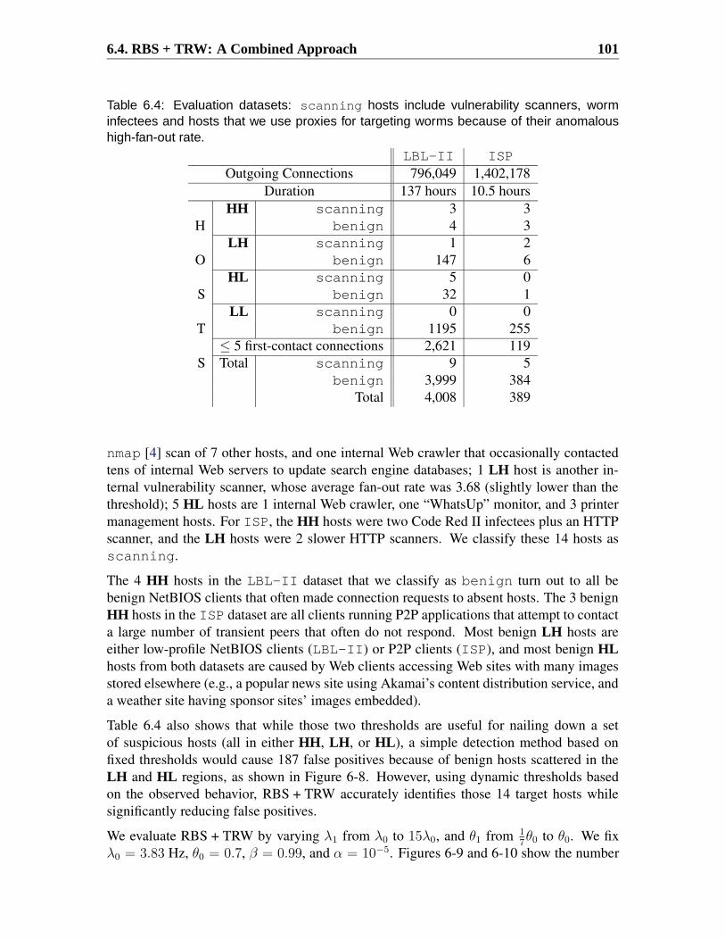
6.4. RBS + TRW: A Combined Approach 101
Table 6.4: Evaluation datasets: scanning hosts include vulnerability scanners, worminfectees and hosts that we use proxies for targeting worms because of their anomaloushigh-fan-out rate.
LBL-II ISPOutgoing Connections 796,049 1,402,178
Duration 137 hours 10.5 hoursHH scanning 3 3
H benign 4 3LH scanning 1 2
O benign 147 6HL scanning 5 0
S benign 32 1LL scanning 0 0
T benign 1195 255≤ 5 first-contact connections 2,621 119
S Total scanning 9 5benign 3,999 384
Total 4,008 389
nmap [4] scan of 7 other hosts, and one internal Web crawler that occasionally contactedtens of internal Web servers to update search engine databases; 1 LH host is another in-ternal vulnerability scanner, whose average fan-out rate was 3.68 (slightly lower than thethreshold); 5 HL hosts are 1 internal Web crawler, one “WhatsUp” monitor, and 3 printermanagement hosts. For ISP, the HH hosts were two Code Red II infectees plus an HTTPscanner, and the LH hosts were 2 slower HTTP scanners. We classify these 14 hosts asscanning.
The 4 HH hosts in the LBL-II dataset that we classify as benign turn out to all bebenign NetBIOS clients that often made connection requests to absent hosts. The 3 benignHH hosts in the ISP dataset are all clients running P2P applications that attempt to contacta large number of transient peers that often do not respond. Most benign LH hosts areeither low-profile NetBIOS clients (LBL-II) or P2P clients (ISP), and most benign HLhosts from both datasets are caused by Web clients accessing Web sites with many imagesstored elsewhere (e.g., a popular news site using Akamai’s content distribution service, anda weather site having sponsor sites’ images embedded).
Table 6.4 also shows that while those two thresholds are useful for nailing down a setof suspicious hosts (all in either HH, LH, or HL), a simple detection method based onfixed thresholds would cause 187 false positives because of benign hosts scattered in theLH and HL regions, as shown in Figure 6-8. However, using dynamic thresholds basedon the observed behavior, RBS + TRW accurately identifies those 14 target hosts whilesignificantly reducing false positives.
We evaluate RBS + TRW by varying λ1 from λ0 to 15λ0, and θ1 from 17θ0 to θ0. We fix
λ0 = 3.83 Hz, θ0 = 0.7, β = 0.99, and α = 10−5. Figures 6-9 and 6-10 show the number

102 Chapter 6. Detection of Targeting Worm Propagations
of detection and false positives for each pair of λ1 and θ1. In particular, for λ1 = λ0, thecombined algorithm reduces to TRW (dashed vertical lines along the θ1 axis), and whenθ1 = θ0, to RBS (dashed vertical lines along the λ0 axis).
Table 6.5: Evaluation of RBS + TRW vs. RBS and TRW: LBL-II has 9 scanners andISP has 5 scanners. N |H1 represents the average number of first-contact connectionsoriginated from the detected hosts upon detection.
LBL-II ISPλ1 θ1 False - False + N |H1 False - False + N |H1
RBS 11λ0 = θ0 0 25 5.6 2 8 6.4TRW = λ0
17θ0 7 5 18.5 0 3 10.0
RBS + TRW 10λ047θ0 1 9 6.9 1 6 5.0
Table 6.5 compares the performance of the combined algorithm against that of RBS andTRW alone. First, we find the priors that make RBS (TRW) the most effective (0 falsenegatives) in identifying scanners in the LBL-II (ISP) dataset. The nature of our testdatasets keeps either algorithm from working better across both datasets. In fact, whenλ1 = 11λ0 and θ1 = θ0, RBS has 0 false negatives for LBL-II, but misses 2 LH scannersin ISP. In comparison, when λ1 = λ0 and θ1 = 1
7θ0, TRW has 0 false negatives for ISP,
but misses 7 scanners in LBL-II, including the HL hosts, 1 Web crawler and the LHnmap scanner.
We could address the problem of false negatives for either algorithm by running TRW andRBS in parallel, raising an alarm if either algorithm decides so. However, this approachcomes at the cost of an increased number of false alarms, which usually result from LHhosts (e.g., Windows NetBIOS connections, often made to absent hosts) or HL hosts (e.g.,a busy mail server or a Web proxy).
In general, improving the accuracy of a detection algorithm requires iterative adjustmentsof decision rules: first improving the detection rate by loosening the decision rule, and thendecreasing the false positive rate by tightening the decision rule without losing too manycorrect detections. For this iteration, our combined algorithm, RBS + TRW provides twoknobs, λ1 and θ1, that we can adjust to tune the detector to a site’s traffic characteristics.
The trace-driven simulation shows that RBS + TRW with λ1 = 10λ0 and θ1 = 47θ0 misses
only two low-profile target hosts (one iprint host from LBL-II and a slow HTTP scannerfrom ISP) while generating no more than 15 false positives, per Table 6.5. Had we runRBS and TRW in parallel, we could have eliminated all the false negatives, but at the costof 41 false alarms altogether.
Overall, RBS + TRW provides the good detection of high-profile worms and scanners (nomore than 2 misses across both datasets) while generating less than 1 false alarm per hourfor a wide range of parameters (λ1 ∈ [10λ0, 15λ0] and θ1 ∈ [4
7θ0,
67θ0]), and reaching its
detection decisions quickly (less than 7 first-contact connections on average).

6.4. RBS + TRW: A Combined Approach 103
λ1
θ1
0 2 4 6 8
10
Detection
λ02λ0
4λ06λ0
8λ010λ0
12λ014λ0
θ0
5θ0/73θ0/7
θ0/7
Detection
(a) Detection (out of 9 targets)
λ1
θ1
0 5
10 15 20 25 30
False positives
λ02λ0
4λ06λ0
8λ010λ0
12λ014λ0
θ0
5θ0/73θ0/7
θ0/7
False positives
(b) False alarms (out of 4,008 hosts)
Figure 6-9: Simulation results of RBS + TRW for the LBL-II dataset, varying λ1 and θ1:each point represents the number of detection or false alarms when the detection algorithmis run with a certain pair of λ1 and θ1. In particular, points connected with the vertical linesalong the θ1 axis are the results when λ1 = λ0 (TRW) and those connected with the verticallines along the λ1 axis are the results when θ1 = θ0 (RBS).

104 Chapter 6. Detection of Targeting Worm Propagations
λ1
θ1
0 1 2 3 4 5
Detection
λ02λ0
4λ06λ0
8λ010λ0
12λ014λ0
θ0
5θ0/73θ0/7
θ0/7
Detection
(a) Detection (out of 5 targets)
λ1
θ1
0 1 2 3 4 5 6 7 8
False positives
λ02λ0
4λ06λ0
8λ010λ0
12λ014λ0
θ0
5θ0/73θ0/7
θ0/7
False positives
(b) False alarms (out of 389 hosts)
Figure 6-10: Simulation results of RBS + TRW for the ISP dataset, varying λ1 and θ1: eachpoint represents the number of detection or false alarms when the detection algorithm isrun with a certain pair of λ1 and θ1. In particular, points connected with the vertical linesalong the θ1 axis are the results when λ1 = λ0 (TRW) and those connected with the verticallines along the λ1 axis are the results when θ1 = θ0 (RBS).

6.5. Discussion 105
6.5 Discussion
This section discusses several technical issues that may arise when employing RBS + TRWin practice. While addressing these issues is beyond the scope of this work, we outlinegeneral ideas and directions.
Operational Issues. A worm detection device running RBS + TRW needs to maintainper local host information. For each host, a detector must track first-contact connectionsoriginated by the host, their failure/success status, and the elapsed time. The state thusincreases proportional to the number of local hosts in the network (N ) and the sum of alltheir currently pending first-contact connections. Given that RBS + TRW requires ≤ 10first-contact connections on average to reach a decision (see Section 6.4), we can estimateamount of state as scaling on the order of 10N . Note that every time RBS + TRW crosseseither threshold, it resets its states for the corresponding host.
When constrained by computation and storage resources, one can employ cache data struc-tures suggested by Weaver et al. [83] that track first-contact connections with a high preci-sion. However, we note that running RBS + TRW on the aggregated traffic across hosts (asopposed to the per-host operation for which it is designed) can significantly affect the de-tection performance due to the uneven traffic distribution generated by each end-host [90].
Post-detection Response. The results in Table 6.5 correspond to RBS + TRW generating0.07 false alarms per hour at the LBL-II site and 0.57 per hour at the ISP site. Thislow rate, coupled with RBS + TRW’s fast detection speed, make it potentially suitable forautomated containment, crucial to defending against fast-spreading worms. Alternatively, anetwork operator could employ connection rate-limiting for hosts detected by RBS + TRW,automatically restricting such hosts to a low fan-out rate.
Limitations. As indicated in Figure 6-8, RBS + TRW is unable to detect targeting wormsusing high-quality hit lists comprised of at least 70% active hosts and spreading no fasterthan several first-contact connections per second. Detecting such worms might be possi-ble by working on larger time scales. For example, a scanner that generates first-contactconnections at a rate of 1 Hz will end up accessing 3,600 different hosts in an hour, faroutnumbering the sustained activity of a typical benign host. Thus, a natural avenue forfuture work is assessing the operation of RBS on longer timescales.
Finally, attackers can game our detection algorithm by tricking end users into generat-ing first-contact connections either at a high rate (RBS), or that will likely end up failing(TRW). For instance, similar to an attack discussed in Section 5.4, an attacker could putcontent on a web site with numerous embedded links to non-existent destinations.
6.6 Summary
We have presented a worm detection algorithm, RBS (Rate-Based Sequential HypothesisTesting), that rapidly identifies high-fan-out behavior by hosts (e.g., targeting worms) basedon the rate at which the hosts initiate connections to new destinations. RBS is built on anempirically-driven probability model that captures benign network characteristics, which
106 Chapter 6. Detection of Targeting Worm Propagations
allows us to discriminate between benign traffic and scanning traffic. Developed using themathematical framework of sequential hypothesis testing [80], RBS can effectively adaptits threshold and window size, based on which it computes instantaneous rates to use inupdating its decision-making in real-time. This gives RBS an essential advantage overschemes using single, fixed values for these.
We have evaluated RBS using trace-driven simulations. We find that when the factor ofspeed difference, n, between a scanner and a benign host is small, RBS requires moreempirical data to arrive at a detection decision; for example, it requires on average 10.4 first-contact connections when n = 5, but the theoretical bound shows that it can detect anyscanners that sustain more than 9.5 first-contact connections per second. In addition, as ngrows larger RBS provides accurate and quick detection.
Finally, we have developed RBS + TRW, a hybrid of RBS and TRW, which combines fan-out rate and probability of success of each first-contact connection. RBS + TRW providesa unified framework for detecting fast-propagating worms independent of their target dis-covery strategy (i.e., targeting worm or scanning worm). Using two traces from two quali-tatively different sites, containing 389 active hosts and 4,008 active hosts, respectively, weshow that RBS + TRW provides fast detection of hosts infected by Code Red II, as well asthe internal Web crawlers and a network monitoring tool that we use as proxies for targetingworms. In doing so, it generates less than 1 false alarm per hour.
Chapter 7
Conclusion and Future Directions
We have investigated three malicious network activities — portscan, scanning worm infec-tion, and targeting worm propagation, and developed detection algorithms that accuratelyidentify a host engaged in such forms of malicious activities in real-time. A common basisof our detection algorithms is an ability to capture connection-level characteristics that areinherent to each activity type. We have shown that there is a disparity between the fre-quency with which connections to newly visited addresses are successful for benign hostsvs. for scanners (Chapters 4 and 5). Another characteristic is the rate at which a host ini-tiates connections to new destinations, which proves useful for identifying high-fan-outbehavior by hosts infected by targeting worms (Chapter 6).
Our algorithms rely on connection-level information (e.g., source and destination IP ad-dresses, protocol, connection status) and do not require access to packet contents. Com-pared to content-based approaches [37, 62, 81], our connection-based approach incurs sig-nificantly lower processing cost when implemented in a detection system. Moreover, pay-load information is not always available (e.g., failed connection attempts), and the increas-ing use of application-level encryption can render content-based approaches ineffective.However, we note that content-based approaches are capable of detecting slow-propagating(stealthy) worms that are indistinguishable from benign hosts in their traffic behavior.
Our study shows that due to the stochastic nature of a host’s network behavior, it is im-portant that a detection algorithm should be able to dynamically adapt its decision-makingbased on observed traffic data. Built on Wald’s mathematical framework of sequential anal-ysis [80], our detection algorithms automatically adjust the number of events to be collectedaccording to the strength of the evidence. Furthermore, the sequential hypothesis testingmethodology enables engineering the detection algorithms to meet false positive and falsenegative targets, rather than triggering when fixed thresholds are crossed.
While sequential analysis provides an underlying structure over which one can developan adaptive real-time detection algorithm, the algorithm’s performance greatly depends onhow well priors model actual benign and malicious network activities. When poor priorsare used, the performance bounds that the sequential analysis provides are no longer valid:false positives can occur because of atypical benign applications whose behavior is similar
107

108 Chapter 7. Conclusion and Future Directions
to what is modeled as malicious. Likewise, false negatives can occur if the a priori modelsof benign activity include some cases of low-profile attack traffic.
In this study, we obtain priors based on the analysis of real network trace data that containvarious types of network traffic as well as the malicious traffic of interest. However, wefind it challenging to find “good” priors that properly separate benign network traffic frommalicious mainly because of the following two reasons.
1. Once a detection algorithm is known, attackers can craft traffic behavior such thattheir attack traffic smears among other legitimate traffic flows. Because of this never-ending arms race between attackers and defense systems, it may be impossible todesign a bullet-proof detection algorithm. Yet, some traffic properties are harder tomodify and therefore work better as priors. In Chapter 4, we show that a strongmodality appears when we look at the ratio of failed connection attempts over thetotal number of connections originated from each remote host. Since a portscannerhas little knowledge of the configuration of a target network, this pattern of frequentlyaccessing non-responding hosts (thus making a connection attempt unsuccessful) ishard to alter.
2. Applications vary a lot in their network behavior, making it difficult to find a reason-ably simple model that captures all benign network activity. As shown in Chapter 6, abenign host’s first-contact connection interarrival times are distributed across a widerange of intervals. However, when focusing on sub-second interarrivals, we find thatthose interarrival times fit an exponential distribution fairly well.
Using real trace data collected from multiple sites, we have evaluated the performanceof our algorithms and examined false alarms and missed detections: our portscan detec-tion algorithm, TRW, is more accurate and requires a much smaller number of events(4 or 5 packets in practice) to detect remote portscanners compared to previous schemessuch as Bro [52] and Snort [56] (Chapter 4). Our credit-based rate limiting algorithm re-sults in significantly fewer unnecessary rate limiting than the virus throttle [76] (Chapter 5).Our worm detection algorithm, RBS + TRW, provides fast detection of hosts infected byCode Red II, as well as hosts exhibiting abnormal level of high fan-out-rate. In doing so,RBS + TRW generates less than 1 false alarm per hour (Chapter 6).
This dissertation demonstrates that, when properly modeled, traffic characteristics can beused for identifying certain malicious network activities with high accuracy. One avenuefor future work includes extending a detection algorithm to further classify the results withapplication-level semantics. For instance, if there is a database available that maintainsinformation about which worms exploit which services, the detection algorithm can triggeran alarm of the “Slammer worm” as opposed to “some worm”, if the detector finds a localhost generating scan traffic to port 1434. Imbuing alarms with such semantics will facilitatethe construction of an appropriate response after detection. If an alarm results from thetraffic from the application in which a critical vulnerability is recently published, it is astrong indicator of a new worm outbreak and thus automatic containment is vital.

109
Finally, this dissertation provides important building blocks toward a general frameworkof categorizing network traffic by the activity being performed at the originating client.If traffic profiles are available for multiple activity types, one can build a classifier thatanalyzes network traffic associated with active hosts and reports their activity in real-time(e.g., worm propagation over port 80, running peer-to-peer applications tunneling throughport 80, benign Web browsing). This kind of classifier will not only protect the networkagainst many known Internet attacks, but also significantly enhance our understanding ofongoing “network situational awareness” [91].


Appendix A
Implementation of TRW in Bro policy
The Bro network intrusion detection system includes a number of policy scripts, whichanalyze network traffic and determine alarm worthy events used by the main program [1].We implemented the Threshold Random Walk (TRW) portscan detection algorithm in Bropolicy. One can load the TRW policy file, trw.bro using the @load command. Below isthe source code of trw.bro.@load a l e r t@load p o r t−name@load h o t@load scan
r e d e f use TRW algor i thm = T ;
r e d e f enum A l e r t + = {TRWAddressScan , # Source f l a g g e d as s c a n n e r by TRW a l g o r i t h mTRWScanSummary , # Summary o f s c a n n i n g a c t i v i t i e s r e p o r t e d by TRW} ;
module TRW;
g l o b a l t a r g e t d e t e c t i o n p r o b = 0 . 9 9 & r e d e f ;g l o b a l t a r g e t f a l s e p o s i t i v e p r o b = 0 . 0 1 & r e d e f ;
# As d e f i n e d i n Chapter 4 , t h e t a z e r o ( t h e t a o n e ) i s t h e s u c c e s s# p r o b a b i l i t y o f a g i v e n b e n i g n ( s c a n n i n g ) remote h o s t ’ s f i r s t# c o n t a c t c o n n e c t i o ng l o b a l t h e t a z e r o = 0 . 8 & r e d e f ;g l o b a l t h e t a o n e = 0 . 1 & r e d e f ;
# S e t o f remote h o s t s s u c c e s s f u l l y a c c e s s e d by l o c a l h o s t sg l o b a l f r i e n d l y r e m o t e s : s e t [ add r ] ;
# S e t o f l o c a l h o n e y p o t h o s t s i f any
111

112 Chapter A. Implementation of TRW in Bro policy
g l o b a l honeypo t : s e t [ add r ] ;
# Upper and lower t h r e s h o l d s : i n i t i a l i z e d when Bro s t a r t sg l o b a l e t a z e r o : d o u b l e ;g l o b a l e t a o n e : d o u b l e ;
# T e l l TRW n o t t o f l a g f r i e n d l y r e m o t e sg l o b a l d o n o t f l a g f r i e n d l y r e m o t e s = T & r e d e f ;
# S e t o f s e r v i c e s o f ou tbound c o n n e c t i o n s t h a t are# p o s s i b l y t r i g g e r e d by incoming c o n n e c t i o n sc o n s t t r i g g e r e d o u t b o u n d s e r v i c e s ={ i d e n t , f i n g e r , 2 0 / t cp , } & r e d e f ;
g l o b a l TRW scan sources : s e t [ add r ] ;g l o b a l TRW benign sources : s e t [ add r ] ;
g l o b a l f i r s t c o n t a c t c o n n e c t i o n s : s e t [ addr , add r ] ;
g l o b a l lambda : t a b l e [ add r ] o f d o u b l e & d e f a u l t = 1 . 0 ;g l o b a l n u m s c a n n e d l o c a l s : t a b l e [ add r ] o f c o u n t & d e f a u l t = 0 ;
e v e n t b r o i n i t ( ) {# Approx imate s o l u t i o n s f o r upper and lower t h r e s h o l d s
e t a z e r o =( 1 − t a r g e t d e t e c t i o n p r o b ) / ( 1 − t a r g e t f a l s e p o s i t i v e p r o b ) ;
e t a o n e = t a r g e t d e t e c t i o n p r o b / t a r g e t f a l s e p o s i t i v e p r o b ;}
e v e n t TRW scan summary ( o r i g : add r ) {ALERT ( [ $ a l e r t =TRWScanSummary , $ s r c = o r i g ,
$msg=fmt ( ”%s scanned a t o t a l o f %d h o s t s ” ,o r i g , n u m s c a n n e d l o c a l s [ o r i g ] ) ] ) ;}
e x p o r t {f u n c t i o n check TRW scan ( c : c o n n e c t i o n , s t a t e : s t r i n g ,r e v e r s e : boo l ) : boo l {
l o c a l i d = c $ i d ;l o c a l s e r v i c e =
( c $ s e r v i c e = = p o r t n a m e s [ 2 0 / t c p ] ) ? 2 0 / t c p : i d $ r e s p p ;l o c a l o r i g = r e v e r s e ? i d $ r e s p h : i d $ o r i g h ;l o c a l r e s p = r e v e r s e ? i d $ o r i g h : i d $ r e s p h ;l o c a l outbound = i s l o c a l a d d r ( o r i g ) ;
# Mark a remote as f r i e n d l y i f i t i s s u c c e s s f u l l y a c c e s s e d by# a l o c a l w i t h p r o t o c o l s o t h e r than t r i g g e r e d o u t b o u n d s e r v i c e s

113
i f ( ou tbound ) {i f ( r e s p ! i n TRW scan sources &&
s e r v i c e ! i n t r i g g e r e d o u t b o u n d s e r v i c e s &&o r i g ! i n honeypo t && s t a t e ! = ”OTH” )add f r i e n d l y r e m o t e s [ r e s p ] ;
re turn F ;}
i f ( o r i g i n TRW scan sources )re turn T ;
i f ( o r i g i n TRW benign sources )re turn F ;
i f ( d o n o t f l a g f r i e n d l y r e m o t e s && o r i g i n f r i e n d l y r e m o t e s )re turn F ;
# S t a r t TRW e v a l u a t i o nl o c a l f l a g = + 0 ;l o c a l r e s p b y t e = r e v e r s e ? c $ o r i g $ s i z e : c $ r e s p $ s i z e ;l o c a l e s t a b l i s h e d = T ;
i f ( s t a t e = = ” S0 ” | | s t a t e = = ”REJ” | | s t a t e = = ”OTH” | |( s t a t e = = ”RSTOS0” && r e s p b y t e < = 0 ) )
e s t a b l i s h e d = F ;
i f ( ! e s t a b l i s h e d | | r e s p i n honeypo t ) {i f ( [ o r i g , r e s p ] ! i n f i r s t c o n t a c t c o n n e c t i o n s ) {
f l a g = 1 ;add f i r s t c o n t a c t c o n n e c t i o n s [ o r i g , r e s p ] ;}}
e l s e i f ( [ o r i g , r e s p ] ! i n f i r s t c o n t a c t c o n n e c t i o n s ) {f l a g = −1 ;add f i r s t c o n t a c t c o n n e c t i o n s [ o r i g , r e s p ] ;}
i f ( f l a g = = 0 )re turn F ;
l o c a l r a t i o = 1 . 0 ;
# Update t h e c o r r e s p o n d i n g l i k e l i h o o d r a t i o o f o r i gi f ( t h e t a z e r o < = 0 | | t h e t a z e r o > = 1 | | t h e t a o n e < = 0 | |
t h e t a o n e > = 1 | | t h e t a o n e >= t h e t a z e r o ) {

114 Chapter A. Implementation of TRW in Bro policy
# Error : t h e t a z e r o s h o u l d be be tween 0 and 1l o g ” bad t h e t a z e r o / t h e t a o n e i n check TRW scan ” ;use TRW algor i thm = F ;re turn F ;}
i f ( f l a g = = 1 )r a t i o = ( 1 − t h e t a o n e ) / ( 1 − t h e t a z e r o ) ;
i f ( f l a g = = −1 )r a t i o = t h e t a o n e / t h e t a z e r o ;
++ n u m s c a n n e d l o c a l s [ o r i g ] ;
lambda [ o r i g ] = lambda [ o r i g ] ∗ r a t i o ;l o c a l u p d a t e d l a m b d a = lambda [ o r i g ] ;
i f ( t a r g e t d e t e c t i o n p r o b < = 0 | |t a r g e t d e t e c t i o n p r o b > = 1 | |t a r g e t f a l s e p o s i t i v e p r o b < = 0 | |t a r g e t f a l s e p o s i t i v e p r o b > = 1 ) {# Error : t a r g e t p r o b a b i l i t i e s s h o u l d be be tween 0 and 1l o g ” bad t a r g e t p r o b a b i l i t i e s i n check TRW scan ” ;use TRW algor i thm = F ;re turn F ;}
i f ( u p d a t e d l a m b d a > e t a o n e ) {add TRW scan sources [ o r i g ] ;ALERT ( [ $ a l e r t =TRWAddressScan , $ s r c = o r i g ,
$msg=fmt ( ”%s scanned a t o t a l o f %d h o s t s ” ,o r i g , n u m s c a n n e d l o c a l s [ o r i g ] ) ] ) ;s c h e d u l e 1 day { TRW scan summary ( o r i g ) } ;re turn T ;
}
i f ( u p d a t e d l a m b d a < e t a z e r o ) {add TRW benign sources [ o r i g ] ;re turn F ;}}}

Bibliography
[1] Bro Intrusion Detection System. http://bro-ids.org. (Cited on pages 78and 111.)
[2] Internet Security Systems — Internet Scanner. http://www.iss.net/products_services/enterprise_protection/vulnerability_assessment/scanner_internet.php. (Cited onpage 16.)
[3] Nessus. http://www.nessus.org/. (Cited on page 16.)
[4] Nmap — Free Security Scanner for Network Exploration & Security Audits.http://www.insecure.org/nmap/. (Cited on pages 16, 30 and 101.)
[5] Novell: iPrint Overview. http://www.novell.com/products/netware/printing/quicklook.html. (Cited on page 96.)
[6] WhatsUp Gold — The Standard for Network Monitoring Systems. http://www.areawidetech.com/whatsup_gold.htm. (Cited on page 95.)
[7] D. Anderson, T. Lunt, H. Javits, A. Tamaru, and A. Valdes. Detecting Unusual Pro-gram Behavior Using the Statistical Components of NIDES. Technical Report SRI-CSL-95-06, SRI Computer Science Laboratory, May 1995. (Cited on page 21.)
[8] Michele Basseville and Igor V. Nikiforov. Detection of Abrupt Changes: Theoryand Application, chapter 4.3: Sequential Analysis. Prentice-Hall, Inc., Upper SaddleRiver, NJ, USA, 1993. (Cited on page 25.)
[9] Vincent Berk, George Bakos, and Robert Morris. Designing a Framework for Ac-tive Worm Detection on Global Networks. In Proceedings of the IEEE InternationalWorkshop on Information Assurance, March 2003. (Cited on pages 35 and 71.)
[10] Vincent Berk, Robert Gray, and George Bakos. Using Sensor Networks and DataFusion for Early Detection of Active Worms. In Proceedings of the SPIE AerosenseConference, April 2003. (Cited on pages 35 and 71.)
[11] CAIDA. CAIDA-Analysis of Code Red. http://www.caida.org/analysis/security/code-red/. (Cited on page 65.)
115

116 BIBLIOGRAPHY
[12] CERT. CERT Advisory CA-2001-26 Nimda Worm. http://www.cert.org/advisories/CA-2001-26.html. (Cited on page 33.)
[13] CERT. “Code Red II:” Another Worm Exploiting Buffer Overflow in IIS In-dexing Service DLL. http://http://www.cert.org/incident_notes/IN-2001-09.html. (Cited on pages 34 and 79.)
[14] Shigang Chen and Yong Tang. Slowing Down Internet Worms. In Proceedings ofthe 24th International Conference on Distributed Computing Systems (ICDCS’04),Tokyo, Japan, March 2004. (Cited on pages 35, 85 and 86.)
[15] CIO Asia. CA Details Sophisticated Web At-tack. http://www.idg.com.sg/ShowPage.aspx?pagetype=2&articleid=1482&pubid=5&issueid=48. (Cited onpage 15.)
[16] Fred Cohen. Computer Viruses: Theory and Experiments. Computers and Security,6(1):22–35, 1987. (Cited on page 32.)
[17] Marco de Vivo, Eddy Carrasco, Germinal Isern, and Gabriela O. de Vivo. A Review ofPort Scanning Techniques. SIGCOMM Computer Communication Review, 29(2):41–48, 1999. (Cited on page 30.)
[18] Sven Dietrich, Neil Long, and David Dittrich. Analyzing Distributed Denial Of Ser-vice Tools: The Shaft Case. In Proceedings of LISA, 2000. (Cited on page 17.)
[19] Holger Dreger, Anja Feldmann, Vern Paxson, and Robin Sommer. Operational Ex-periences with High-Volume Network Intrusion Detection. In Proceedings of the11th ACM Conference on Computer and Communications Security, 2004. (Cited onpage 20.)
[20] Mark Eichin and Jon Rochlis. With Microscope and Tweezers: An Analysis of the In-ternet Virus of November 1988. In Proceedings of the IEEE Symposium on Researchin Security and Privacy, 1989. (Cited on pages 32 and 86.)
[21] F-Secure. F-Secure Virus Description Database. http://www.f-secure.com/v-descs/. (Cited on page 32.)
[22] F-Secure. F-Secure Virus Descriptions : Santy. http://www.f-secure.com/v-descs/santy_a.shtml. (Cited on page 86.)
[23] F-Secure Computer Virus Information page. LoveLetter. http://www.f-secure.com/v-descs/love.shtml. (Cited on page 33.)
[24] F-Secure Computer Virus Information page. Lovesan. http://www.f-secure.com/v-descs/msblast.shtml. (Cited on pages 34, 65 and 79.)
[25] F-Secure Computer Virus Information page. Mimail.J. http://www.f-secure.com/v-descs/mimail_j.shtml. (Cited on page 79.)

BIBLIOGRAPHY 117
[26] F-Secure Computer Virus Information page. Mydoom. http://www.f-secure.com/v-descs/novarg.shtml. (Cited on pages 34 and 79.)
[27] F-Secure Computer Virus Information page. Nimda. http://www.f-secure.com/v-descs/nimda.shtml. (Cited on page 33.)
[28] F-Secure Computer Virus Information page. Zotob.A. http://www.f-secure.com/v-descs/zotob_a.shtml. (Cited on page 34.)
[29] Nick Feamster, Jaeyeon Jung, and Hari Balakrishnan. An Empirical Study of “Bogon”Route Advertisements. In Computer Communication Review, Volume 35, Number 1,January 2005. (Cited on page 65.)
[30] Simson Garfinkel, Gene Spafford, and Alan Schwartz. Practical UNIX & InternetSecurity, chapter 5.5: SUID. O’Reilly Media, Inc., Sebastopol, CA, 3rd edition,February 2003. (Cited on page 21.)
[31] Anup K. Ghosh, Aaron Schwartzbard, and Michael Schatz. Learning Program Be-havior Profiles for Intrusion Detection. In Proceedings of the 1st USENIX Workshopon Intrusion Detection and Network Monitoring, April 1999. (Cited on page 21.)
[32] HackFix. SubSeven Removals. http://www.hackfix.org/subseven.(Cited on page 20.)
[33] L. Todd Heberlein, Gihan Dias, Karl Levitt, Biswanath Mukherjee, Jeff Wood, andDavid Wolber. A Network Security Monitor. In Proceedings of the IEEE Symposiumon Research in Security and Privacy, 1990. (Cited on page 30.)
[34] Koral Ilgun, Richard A. Kemmerer, and Phillip A. Porras. State Transition Analysis:A Rule-Based Intrusion Detection Approach. Software Engineering, 21(3):181–199,1995. (Cited on page 20.)
[35] Don Johnson. Criteria in Hypothesis Testing. http://cnx.rice.edu/content/m11228/latest/. (Cited on pages 25 and 26.)
[36] Jaeyeon Jung, Vern Paxson, Arthur W. Berger, and Hari Balakrishnan. Fast PortscanDetection Using Sequential Hypothesis Testing. In Proceedings of the IEEE Sympo-sium on Security and Privacy, May 2004. (Cited on page 22.)
[37] Hyang-Ah Kim and Brad Karp. Autograph: Toward Automated Distributed WormSignature Detection. In Proceedings of the 13th USENIX Security Symposium, Au-gust 9–13, 2004. (Cited on pages 35 and 107.)
[38] C. Ko, M. Ruschitzka, and K. Levitt. Execution Monitoring of Security-Critical Pro-grams in Distributed Systems: a Specification-Based Approach. In Proceedings ofthe IEEE Symposium on Security and Privacy, 1997. (Cited on page 21.)
[39] Sandeep Kumar and Eugene H. Spafford. A Pattern Matching Model for Misuse Intru-sion Detection. In Proceedings of the 17th National Computer Security Conference,1994. (Cited on page 20.)

118 BIBLIOGRAPHY
[40] Christopher Leckie and Ramamohanarao Kotagiri. A Probabilistic Approach to De-tecting Network Scans. In Proceedings of the 8th IEEE Network Operations andManagement Symposium (NOMS 2002), pages 359–372, Florence, Italy, April 2002.(Cited on page 31.)
[41] Ulf Lindqvist and Phillip A Porras. Detecting Computer and Network MisuseThrough the Production-Based Expert System Toolset (P-BEST). In Proceedingsof the 1999 IEEE Symposium on Security and Privacy, pages 146–161, Oakland, Cal-ifornia, may 1999. IEEE Computer Society Press, Los Alamitos, California. (Citedon page 20.)
[42] Matthew V. Mahoney and Philip K. Chan. Learning Nonstationary Models of NormalNetwork Traffic for Detecting Novel Attacks. In Proceedings ACM SIGKDD interna-tional conference on Knowledge discovery and data mining, NY, USA, 2002. (Citedon page 21.)
[43] Jelena Mirkovic, Sven Dietrich, David Dittrich, and Peter Reiher. Internet Denialof Service: Attack and Defense Mechanisms. Prentice Hall PTR, 2004. (Cited onpage 17.)
[44] David Moore, Vern Paxson, Stefan Savage, Colleen Shannon, Stuart Staniford, andNicholas Weaver. Inside the Slammer worm. IEEE Security and Privacy, 1:33–39,July 2003. (Cited on pages 15, 29, 34 and 65.)
[45] David Moore and Colleen Shannon. The Spread of the Code-Red Worm(CRv2). http://www.caida.org/analysis/security/code-red/coderedv2_analysis.xml. (Cited on pages 33 and 65.)
[46] David Moore, Colleen Shannon, Geoffrey M. Voelker, and Stefan Savage. InternetQuarantine: Requirements for Containing Self-Propagating Code. In Proceedings ofIEEE INFOCOM, April 2003. (Cited on pages 34 and 66.)
[47] Robert Morris and Ken Thompson. Password Security: A Case History. Communi-cations of the ACM, 22(11):594–597, 1979. (Cited on page 17.)
[48] George Moustakides. Optimal Procedures for Detecting Changes in Distributions.Annals Statistics, 14:1379–1387, 1986. (Cited on pages 22 and 35.)
[49] Peter G. Neumann. Risks of Passwords. Communications of the ACM, 37(4), 1994.(Cited on page 17.)
[50] Openwall Project. John The Ripper. http://www.openwall.com/john/.(Cited on page 17.)
[51] Martin Overton. Bots and Botnets: Risks, Issues and Prevention. In Proceedings ofthe 15th Virus Bulletin Conference, 2005. (Cited on page 17.)
BIBLIOGRAPHY 119
[52] Vern Paxson. Bro: a System for Detecting Network Intruders in Real-Time. ComputerNetworks (Amsterdam, Netherlands: 1999), 31(23–24):2435–2463, 1999. (Cited onpages 20, 31, 78, 95 and 108.)
[53] J. B. Postel. Transmission Control Protocol, September 1981. RFC 793. (Cited onpage 30.)
[54] Thomas H. Ptacek and Timothy N. Newsham. Insertion, Evasion, and Denial ofService: Eluding Network Intrusion Detection. Technical report, Suite 330, 1201 5thStreet S.W, Calgary, Alberta, Canada, T2R-0Y6, 1998. (Cited on page 20.)
[55] Seth Robertson, Eric V. Siegel, Matt Miller, and Salvatore J. Stolfo. SurveillanceDetection in High Bandwidth Environments. In Proceedings of the 2003 DARPADISCEX III Conference, Washington, DC, April 2003. (Cited on pages 31 and 68.)
[56] Martin Roesch. Snort: Lightweight Intrusion Detection for Networks. In Proceedingsof the 13th Conference on Systems Administration (LISA-99), Berkeley, CA, Novem-ber 1999. USENIX Association. (Cited on pages 20, 30 and 108.)
[57] Stuart E. Schechter, Jaeyeon Jung, and Arthur W. Berger. Fast Detection of Scan-ning Worm Infections. In Proceedings of the 7th International Symposium on RecentAdvances in Intrusion Detection (RAID 2004), September 2004. (Cited on page 23.)
[58] R. Sekar and P. Uppuluri. Synthesizing Fast Intrusion Prevention/Detection Systemsfrom High-Level Specifications. In Proceedings of the 8th USENIX Security Sympo-sium, 1999. (Cited on page 21.)
[59] Colleen Shannon and David Moore. The Spread of the Witty Worm. Technical report,Cooperative Association for Internet Data Analysis (CAIDA), March 2004. (Cited onpages 34 and 65.)
[60] Stelios Sidiroglou and Angelos D. Keromytis. A Network Worm Vaccine Architec-ture. In Proceedings of the IEEE International Workshops on Enabling Technologies:Infrastructure for Collaborative Enterprises (WETICE), Workshop on Enterprise Se-curity, June 2003. (Cited on page 66.)
[61] Stelios Sidiroglou and Angelos D. Keromytis. Countering Network Worms ThroughAutomatic Patch Generation. In Proceedings of the IEEE Symposium on Security andPrivacy, 2005. (Cited on page 66.)
[62] Sumeet Singh, Cristian Estan, George Varghese, and Stefan Savage. AutomatedWorm Fingerprinting. In Proceedings of the 13th Operating Systems Design andImplementation OSDI, December 2004. (Cited on pages 35 and 107.)
[63] Eugene H. Spafford. A Failure to Learn from the Past. In Proceedings of the 19thAnnual Computer Security Applications Conference, pages 217–233, December 2003.(Cited on pages 32 and 86.)

120 BIBLIOGRAPHY
[64] @stake. L0phtCrack. http://www.atstake.com/products/lc/. (Citedon page 17.)
[65] Stuart Staniford. Containment of Scanning Worms in Enterprise Networks. Journalof Computer Security, Forthcoming. (Cited on page 35.)
[66] Stuart Staniford, James A. Hoagland, and Joseph M. McAlerney. Practical Auto-mated Detection of Stealthy Portscans. In Proceedings of the 7th ACM Conference onComputer and Communications Security, Athens, Greece, 2000. (Cited on pages 32and 58.)
[67] Stuart Staniford, Vern Paxson, and Nicholas Weaver. How to 0wn the Internet in YourSpare Time. In Proceedings of the 11th USENIX Security Symposium, Berkeley, CA,USA, August 2002. (Cited on page 86.)
[68] S. Staniford-Chen, S. Cheung, R. Crawford, M. Dilger, J. Frank, J. Hoagland,K. Levitt, C. Wee, R. Yip, and D. Zerkle. GrIDS – A Graph-based Intrusion De-tection System for Large Networks. In Proceedings of the 19th National InformationSystems Security Conference, volume 1, pages 361–370, October 1996. (Cited onpages 35 and 84.)
[69] Symantec. Security Response – Code Red II. http://securityresponse.symantec.com/avcenter/venc/data/codered.ii.html. (Cited onpages 29, 34 and 79.)
[70] Symantec. Symantec Internet Security Threat Report Identifies More Attacks NowTargeting e-Commerce, Web Applications. http://www.symantec.com/press/cgi/printfriendlypress.cgi?release=2004/n040920b.html. (Cited on page 15.)
[71] Symantec Security Response. Search and Latest Virus Threats. http://www.symantec.com/avcenter/vinfodb.html. (Cited on page 32.)
[72] Symantec Security Response. W32.Nimda.A@mm. http://securityresponse.symantec.com/avcenter/venc/data/[email protected]. (Cited on page 33.)
[73] Symantec Security Response. W32.Sasser.Worm. http://securityresponse.symantec.com/avcenter/venc/data/w32.sasser.worm.html. (Cited on page 65.)
[74] silicon.com. Denial of Service Attack Victim Speaks Out. http://http://management.silicon.com/smedirector/0,39024679,39130810,00.htm, 2005. (Cited on page 17.)
[75] The Internet Assigned Numbers Authority. Port Numbers. http://http://www.iana.org/assignments/port-numbers/, last accessed on February1, 2006. (Cited on page 79.)

BIBLIOGRAPHY 121
[76] Jamie Twycross and Matthew M. Williamson. Implementing and Testing a VirusThrottle. In Proceedings of the 12th USENIX Security Symposium, August 2003.(Cited on pages 13, 35, 66, 75, 78, 80, 85, 88 and 108.)
[77] United States Computer Emergency Readiness Team. US-CERT Vulnerability Notes.http://www.kb.cert.org/vuls/. (Cited on page 17.)
[78] USA TODAY. Unprotected PCs can be Hijacked in Minutes.http://www.usatoday.com/money/industries/technology/2004-11-29-honeypot_x.htm. (Cited on page 15.)
[79] Luis von Ahn, Manuel Blum, and John Langford. Telling Humans and ComputersApart (Automatically) or How Lazy Cryptographers Do AI. Technical Report CMU-CS-02-117, February 2002. (Cited on page 80.)
[80] Abraham Wald. Sequential Analysis. J. Wiley & Sons, New York, 1947. (Cited onpages 18, 21, 26, 48, 50, 54, 92, 106 and 107.)
[81] Ke Wang, Gabriela Cretu, and Salvatore J. Stolfo. Anomalous payload-based wormdetection and signature generation. In Proceedings of the Eighth International Sym-posium on Recent Advances in Intrusion Detection (RAID 2005), September 2005.(Cited on page 107.)
[82] Nicholas Weaver, Vern Paxson, Stuart Staniford, and Robert Cunningham. A Taxon-omy of Computer Worms. In Proceedings of the ACM Workshop on Rapid Malcode,Washington, DC, 2003. (Cited on pages 65, 86 and 99.)
[83] Nicholas Weaver, Stuart Staniford, and Vern Paxson. Very Fast Containment of Scan-ning Worms. In Proceedings of the 13th USENIX Security Symposium, August 2004.(Cited on pages 35, 83, 84, 86, 97 and 105.)
[84] David Whyte, Evangelos Kranakis, and P.C. van Oorschot. DNS-based Detection ofScanning Worms in an Enterprise Network. In Proceedings of the Network and Dis-tributed System Security Symposium (NDSS’05), February 2005. (Cited on pages 35and 86.)
[85] Wikipedia. Mydoom. http://en.wikipedia.org/wiki/MyDoom, last ac-cessed on February 10, 2006. (Cited on pages 34 and 79.)
[86] Wikipedia. SQL Slammer Worm. http://en.wikipedia.org/wiki/SQL_slammer_worm, last accessed on February 10, 2006. (Cited on page 65.)
[87] Wikipedia. Timeline of Notable Computer Viruses and Worms. http://en.wikipedia.org/wiki/Notable_computer_viruses_and_worms, lastaccessed on February 10, 2006. (Cited on page 32.)
[88] Wikipedia. Zotob. http://en.wikipedia.org/wiki/Zotob, last accessedon February 10, 2006. (Cited on page 34.)
122 BIBLIOGRAPHY
[89] Matthew M. Williamson. Throttling Viruses: Restricting Propagation to Defeat Mali-cious Mobile Code. In Proceedings of The 18th Annual Computer Security Applica-tions Conference (ACSAC 2002), December 2002. (Cited on pages 35, 66 and 75.)
[90] Cynthia Wong, Stan Bielski, Ahren Studer, and Chenxi Wang. Empirical Analysis ofRate Limiting Mechanisms. In Proceedings of the Eighth International Symposiumon Recent Advances in Intrusion Detection (RAID 2005), September 2005. (Cited onpage 105.)
[91] Vinod Yegneswaran, Paul Barford, and Vern Paxson. Using Honeynets for InternetSituational Awareness. In Proceedings of ACM Sigcomm Hotnets, 2005. (Cited onpage 109.)
[92] T. Ylonen and C. Lonvick Ed. The Secure Shell (SSH) Protocol Architecture. InternetEngineering Task Force, January 2006. RFC 4251. (Cited on page 17.)