real-time machine listening and segmental re-synthesis for
TRANSCRIPT
Real-time Machine Listening
and Segmental Re-synthesis
for Networked Music Performance
Dissertation
zur Erlangung der Würde des
Doktors der Philosophie
des Fachbereichs Kulturgeschichte
und Kulturkunde
der Universität Hamburg
vorgelegt von
Chrisoula Alexandraki
aus Athen, Griechenland
Hamburg, 2014
2
1. Gutachter: Herr Prof. Dr. Rolf Bader
2. Gutachter: Herr Prof. Dr. Albrecht Schneider
Datum der Disputation:
17. November 2014
Tag des Vollzugs der Promotion:
26. November 2014
3
Abstract
The general scope of this work is to investigate potential benefits of Networked Music
Performance (NMP) systems by employing techniques commonly found in Machine
Musicianship. Machine Musicianship is a research area aiming at developing software
systems exhibiting some musical skill such as listening, composing or performing
music. A distinct track of this research line, mostly relevant to this work, is computer
accompaniment systems. Such systems are expected to accompany human musicians by
causally analysing the music being performed and timely responding by synthesizing an
accompaniment, or the part of one or more of the remaining members of a performance
ensemble. The objective of the present work is to investigate the possibility of
representing each performer of a dispersed NMP ensemble, by a local computer-based
musician, which constantly listens to the local performance, receives network
notifications from remote locations and re-synthesizes the performance of remote peers.
Whenever a new musical construct is recognized at the location of each performer, a
code representing that construct is communicated to all of the remaining musicians, as
low-bandwidth information. Upon reception, the remote audio signal is re-synthesized
by splicing pre-recorded audio segments corresponding to the musical construct
identified by the received code. Computer accompaniment systems may use any
conventional audio synthesis technique to generate the accompaniment. In this work,
investigations focus on concatenative music synthesis, in an attempt to preserve all
expressive nuances introduced by the interpretation of individual performers. Hence, the
research carried out and presented in this dissertation lies on the intersection of three
domains, which are NMP, Machine Musicianship and Concatenative Music Synthesis.
The dissertation initially presents an analysis of the current trends in all three research
domains, and then elaborates on the methodology that was followed to realize the
intended scenario. Research efforts have led to the development of BoogieNet, a
preliminary software prototype implementing the proposed communication scheme for
networked musical interactions. Real-time music analysis is achieved by means of
audio-to-score alignment techniques and re-synthesis at the receiving end takes place by
concatenating pre-recorded and automatically segmented audio units, generated by
means of onset detection algorithms. The methodology of the entire process is presented
and contrasted with competing analysis/synthesis techniques. Finally, the dissertation
presents important implementation details and an experimental evaluation to
demonstrate the feasibility of the proposed approach.
4
Acknowledgements
First of all, I want to thank my advisor Prof. Rolf Bader for his valuable guidance,
continuous help, encouragement, inspiration and understanding during all phases of my
doctorate research.
I would also like to thank the members of the examining committee: Prof. Albrecht
Schneider for thoroughly reviewing this dissertation, and also Prof. Georg Hajdu, Prof.
Christiane Neuhaus and Prof. Udo Zölzer for their time and expertise.
Many thanks to my friend and former classmate Esben Skovenborg for helping me to
disambiguate some audio signal processing concepts and for reviewing certain chapters
of this dissertation.
I owe a great thank you to my colleague Prof. Demosthenes Akoumianakis for his
continuous encouragement and support to pursue my research visions.
When thinking over the last few years, I think the most difficult part of this work was to
define the precise research problem I wanted tackle. In trying to solve this puzzle, I had
the valuable support of my former colleague Alexandros Paramythis. Although
researching in different domains, he suggested some key concepts that helped me to
determine what I really wanted to do. So, I want to deeply thank him for that!
There are also two people living in the beautiful city of Hamburg that I would like to
thank: Prof. George Hajdu, whom I first met in Belfast during the 2008 International
Computer Music Conference (ICMC), for suggesting me to work with Prof. Bader and
for all our interesting discussions on Networked Music Performance. I also want to
thank Konstantina Orlandatou for welcoming me in Hamburg and for helping me cope
with the administrative regulations of the University of Hamburg.
Many thanks also go to my colleague Panagiotis Zervas for his patience when I had to
give second priority to our common work obligations. I also owe gratitude to additional
members of academic and administration staff of the Technological Educational
Institute of Crete, who helped to take a sabbatical leave from my position at the
Department of Music Technology and Acoustics Engineering. This possibility has
greatly helped me to complete this work within a reasonable period of time. Special
thanks to Evangelos Kapetanakis, Nektarios Papadogiannis and Georgia Kokkineli.
Last but not least, I want to express my deepest gratitude and love to my mother Poppi
and my brother Dionysis, for understanding my stress and frustration during the last few
years.
Finally, I want to dedicate this work to the memory of my father Lazaros.

5
6
Table of Contents
1 INTRODUCTION ...................................................................................................................... 14
1.1 FROM SCORE TO AUDIO-BASED MUSICAL ANALYSIS................................................................ 15
1.2 TEXTURE, DEVIATIONS AND LEVELS OF MUSIC PERFORMANCE ................................................ 16
1.3 MUSICAL ANTICIPATION IN ENSEMBLE PERFORMANCE ........................................................... 17
1.4 COLLABORATIVE PERFORMANCE ACROSS DISTANCE .............................................................. 18
1.5 DISSERTATION STRUCTURE ................................................................................................... 19
PART I: RELATED WORK .............................................................................................................. 21
2 NETWORKED MUSIC PERFORMANCE .............................................................................. 22
2.1 EARLY ATTEMPTS AND FOLLOW-UP ADVANCEMENTS ............................................................. 22
2.2 RESEARCH CHALLENGES ....................................................................................................... 23
2.3 REALISTIC VS. NON-REALISTIC NMP..................................................................................... 24
2.4 LATENCY TOLERANCE IN ENSEMBLE PERFORMANCE............................................................... 25
2.5 FUNDAMENTALS OF NMP SYSTEM DEVELOPMENT ................................................................. 27
2.5.1 Software applications ...................................................................................................... 27
2.5.1.1 Client Software .................................................................................................................... 28
2.5.1.2 Server Software .................................................................................................................... 30
2.5.2 Network infrastructures ................................................................................................... 31
2.5.2.1 QoS issues ........................................................................................................................... 31
2.5.2.1.1 Network throughput ......................................................................................................... 31
2.5.2.1.2 Latency and Jitter............................................................................................................. 31
2.5.2.1.3 Packet Loss ..................................................................................................................... 32
2.5.2.2 Network protocols ................................................................................................................ 33
2.6 OPEN ISSUES IN NMP RESEARCH ........................................................................................... 36
3 MACHINE MUSICIANSHIP .................................................................................................... 39
3.1 MACHINE LISTENING APPROACHES ....................................................................................... 39
3.2 MUSIC LISTENING AND RELEVANT COMPUTATIONAL AFFORDANCES ....................................... 43
3.2.1 Automatic music transcription ......................................................................................... 44
3.2.2 Audio-to-score alignment ................................................................................................. 46
3.2.3 Audio-to-audio alignment ................................................................................................ 48
3.2.4 Computer accompaniment and robotic performance ......................................................... 49
3.3 MACHINE MUSICIANSHIP IN THE CONTEXT OF NMP ............................................................... 51
4 CONCATENATIVE MUSIC SYNTHESIS............................................................................... 54
4.1 GENERAL METHODOLOGY ..................................................................................................... 54
4.1.1 Audio segmentation ......................................................................................................... 56
4.1.2 Segment analysis and tagging .......................................................................................... 57
4.1.3 Target analysis ................................................................................................................ 58
4.1.4 Matching (Unit Selection) ................................................................................................ 58
4.1.5 Concatenation ................................................................................................................. 59
4.2 CONCATENATION IN SPEECH SYNTHESIS AND CODING ............................................................ 59
4.3 CONTEMPORARY RELEVANT INITIATIVES .............................................................................. 61
4.3.1 Compositional approaches ............................................................................................... 62
7
4.3.1.1 Jamming with Plunderphonics .............................................................................................. 62
4.3.1.2 CataRT ................................................................................................................................ 63
4.3.1.3 Input-Driven explorative synthesis ........................................................................................ 63 4.3.2 High fidelity instrumental simulation ............................................................................... 64
4.3.2.1 Expressive Performance of monophonic Jazz Recordings ...................................................... 64
4.3.2.2 Synful Orchestra................................................................................................................... 65
4.3.2.3 Vocaloid .............................................................................................................................. 65
4.4 COMPARISON WITH THE PRESENT WORK ................................................................................ 66
PART II: RESEARCH METHODOLOGY ....................................................................................... 68
5 RESEARCH FOCUS AND SYSTEM OVERVIEW ................................................................. 69
5.1 RATIONALE AND OBJECTIVE ................................................................................................. 69
5.2 COMPUTATIONAL CHALLENGES ............................................................................................ 70
5.2.1 Real-time constraints ....................................................................................................... 70
5.2.2 Audio quality constraints ................................................................................................. 72
5.3 ASSUMPTIONS - PREREQUISITES ............................................................................................ 73
5.4 ADOPTED METHODOLOGY .................................................................................................... 74
6 ONLINE AUDIO FEATURE EXTRACTION .......................................................................... 77
6.1 FEATURE EXTRACTION AND VISUALISATION .......................................................................... 77
6.2 MATHEMATICAL NOTATION .................................................................................................. 79
6.3 A NOTE ON FREQUENCY TRANSFORMS ................................................................................... 79
6.4 ENERGY FEATURES .............................................................................................................. 87
6.4.1 Energy (E) ....................................................................................................................... 87
6.4.2 RMS amplitude ................................................................................................................ 87
6.4.3 Log Energy (LE) .............................................................................................................. 88
6.5 ONSET FEATURES ................................................................................................................. 89
6.5.1 High Frequency Content (HFC) ....................................................................................... 89
6.5.2 Spectral Activity (SA) ....................................................................................................... 90
6.5.3 Spectral Flux (SF) ........................................................................................................... 91
6.5.4 Phase Deviation (PD) ...................................................................................................... 93
6.5.5 Complex Domain Distance (CDD) ................................................................................... 94
6.5.6 Modified Kullback-Leibler Divergence (MKLD) ............................................................... 95
6.6 PITCH FEATURES .................................................................................................................. 96
6.6.1 Wavelet Pitch (WP) ......................................................................................................... 97
6.6.2 Peak-Structure Match (PSM) ........................................................................................... 98
7 OFFLINE AUDIO SEGMENTATION ................................................................................... 100
7.1 BLIND VS. BY-ALIGNMENT APPROACHES .............................................................................. 100
7.2 ONSETS AND TRANSIENT PHENOMENA ................................................................................. 101
7.3 TYPICAL BLIND ONSET DETECTION METHODOLOGY .............................................................. 104
7.3.1 Pre-processing .............................................................................................................. 105
7.3.2 Reduction ...................................................................................................................... 105
7.3.3 Peak-picking.................................................................................................................. 109
7.4 OFFLINE SEGMENTATION IN THE PROPOSED SYSTEM ............................................................. 110
7.4.1 A Robust onset detection algorithm ................................................................................ 110
7.4.2 Generating Segment Descriptions .................................................................................. 112

8
8 HMM SCORE FOLLOWING ................................................................................................. 113
8.1 THE HMM APPROACH ........................................................................................................ 113
8.2 MATHEMATICAL FOUNDATION ........................................................................................... 115
8.2.1 Definition of an HMM.................................................................................................... 115
8.2.2 Hypothesis and computational approach ........................................................................ 115
8.3 DESIGN CONSIDERATIONS ................................................................................................... 117
8.3.1 States, transitions and HMM topologies ......................................................................... 117
8.3.2 Observations and observation Probabilities ................................................................... 120
8.3.3 Training Process ........................................................................................................... 122
8.3.3.1 Multiple observation sequences........................................................................................... 124
8.3.3.2 Obtaining an initial alignment ............................................................................................. 125
8.3.3.3 Numerical instability .......................................................................................................... 126
8.3.3.4 Memory Requirements ....................................................................................................... 126
8.3.4 Decoding Process .......................................................................................................... 127
8.4 HMM IN THE PROPOSED SYSTEM ......................................................................................... 129
8.4.1 Offline HMM training .................................................................................................... 129
8.4.2 Real-time HMM Decoding ............................................................................................. 131
9 SEGMENTAL RE-SYNTHESIS ............................................................................................. 133
9.1 RENDERING EXPRESSIVE MUSICAL PERFORMANCE ............................................................... 133
9.2 TECHNICAL APPROACHES TO SEGMENTAL RE-SYNTHESIS...................................................... 135
9.2.1 Segment transformations................................................................................................ 136
9.2.1.1 Phase Vocoder Transformations .......................................................................................... 137
9.2.1.2 SOLA transformations ........................................................................................................ 139 9.2.2 Eliminating perceptual discontinuities ........................................................................... 140
9.2.3 Real-time approaches and the need for anticipation ....................................................... 141
9.3 SYNTHESIS IN THE PRESENT SYSTEM .................................................................................... 142
9.3.1 Performance Monitoring and future event estimation ..................................................... 144
9.3.2 Segment Transformations............................................................................................... 145
9.3.3 Concatenation ............................................................................................................... 150
PART III: IMPLEMENTATION & VALIDATION ...................................................................... 152
10 THE BOOGIENET SOFTWARE PROTOTYPE ................................................................... 153
10.1 SOFTWARE AVAILABILITY ................................................................................................... 153
10.2 USING BOOGIENET ............................................................................................................. 154
10.2.1 Offline Audio Segmentation (oas)............................................................................... 155
10.2.2 Performance Model Acquisition (pma) ....................................................................... 156
10.2.3 Train Performance Model (tpm) ................................................................................ 157
10.2.4 Offline Audio to Score Alignment (oasa) .................................................................... 157
10.2.5 Real-time analysis/synthesis (rtas): single-peer .......................................................... 158
10.2.6 Real-time UDP communication (udp): udp-peer......................................................... 162
10.3 SYSTEM OVERVIEW ............................................................................................................ 164
10.3.1 C++ Classes ............................................................................................................. 164
10.3.2 Data Files ................................................................................................................. 166
10.3.2.1 ARFF File .......................................................................................................................... 166
10.3.2.2 Model file .......................................................................................................................... 167
10.3.2.3 Performance Description file............................................................................................... 169
9
10.4 THIRD PARTY LIBRARIES .................................................................................................... 170
11 EXPERIMENTAL EVALUATION ........................................................................................ 172
11.1 CONSIDERATIONS ON THE EVALUATION METHODOLOGY ...................................................... 172
11.1.1 The lack of a formal user evaluation .......................................................................... 172
11.1.2 Standard evaluation metrics and significance of results .............................................. 173
11.1.3 Lack of multiple training sequences ........................................................................... 174
11.1.4 Algorithm fine tuning ................................................................................................. 175
11.2 EVALUATION OF ALGORITHMIC PERFORMANCE .................................................................... 175
11.2.1 Dataset...................................................................................................................... 176
11.2.2 Measures ................................................................................................................... 178
11.2.3 Experimental setup .................................................................................................... 180
11.2.4 Offline Audio Segmentation (OAS) ............................................................................. 181
11.2.5 Real-time Audio to Score Alignment ........................................................................... 184
11.2.5.1 Results prior to HMM training (RTAS-INIT) ...................................................................... 184
11.2.5.2 Results after HMM training (RTAS-TRAINED).................................................................. 187 11.2.6 Comparison of Results ............................................................................................... 189
11.2.7 On the performance of segmental re-synthesis ............................................................ 191
11.3 NETWORK EXPERIMENT ...................................................................................................... 192
11.3.1 Bandwidth consumption ............................................................................................. 194
11.3.2 Network latency and jitter .......................................................................................... 196
11.3.3 The effect of packet loss ............................................................................................. 197
11.4 CONSOLIDATION OF RESULTS .............................................................................................. 197
12 CONCLUSIONS ...................................................................................................................... 201
12.1 SUMMARY AND CONCLUDING REMARKS .............................................................................. 201
12.2 CONTRIBUTIONS ................................................................................................................. 207
12.3 IMPLICATIONS, SHORTCOMINGS AND FUTURE PERSPECTIVES ................................................ 208
13 APPENDIX: NUMERICAL DATA OBTAINED IN THE EVALUATION EXPERIMENTS
212
14 REFERENCES......................................................................................................................... 217
10
List of Figures
Figure 2-1: Typical components of an NMP client application. .............................................................. 28 Figure 2-2: Peer-to-peer vs. centralised media communication in NMP. ................................................ 30 Figure 2-3: The format of the IP header................................................................................................. 33 Figure 2-4: The format of the UDP header. ........................................................................................... 34 Figure 2-5: Structure of an Ethernet frame carrying an RTP packet. The numbers indicate the minimum
size for each header. ..................................................................................................................... 35 Figure 2-6: A GUI offering virtual collaboration capabilities in NMP. ................................................... 37 Figure 3-1: Perception, reasoning and action in machine listening systems. ........................................... 42 Figure 4-1: Data-flow of processes taking place prior to synthesis ......................................................... 55 Figure 4-2: Data-flow of processes taking place during synthesis ........................................................... 56 Figure 4-3: Classification of text-to-speech synthesis techniques ........................................................... 59 Figure 5-1: Block diagram of the processes that take place offline, prior to collaborative performance. .. 74 Figure 5-2: Block diagram of the processes taking place during live NMP. ............................................ 75 Figure 6-1: The musical score of the audio signal used for visualising the values of the audio features. .. 78 Figure 6-2: The windowing function delays the detection of the onset on subsequent hops, resulting in
detection latency corresponding to approximately 30-4 hops. ........................................................ 81 Figure 6-3: Waveform derived from a piano recording. Two 4096-point windows are chosen to
demonstrate the behaviour of STFT during a nearly periodic portion of a signal and a portion for
which a note onset occurs at the last 512 samples representing the hop. ......................................... 82 Figure 6-4: Different parameterisations of the STFT for the nearly periodic segment of the piano signal
shown on Figure 6-3. .................................................................................................................... 85 Figure 6-5: Different parameterisations of the STFT for the segment of the piano signal that contains a
note onset as shown on Figure 6-3. ............................................................................................... 86 Figure 6-6: Temporal evolution of the Energy feature and its first order difference for a short musical
phrase performed by a flute. ......................................................................................................... 87 Figure 6-7: Temporal evolution of the RMS amplitude feature and its first order difference for a short
musical phrase performed by a flute. ............................................................................................ 88 Figure 6-8: Temporal evolution of the Log Energy feature and its first order difference for a short musical
phrase performed by a flute. ......................................................................................................... 89 Figure 6-9: Temporal evolution of the HFC feature and its first order difference for a short musical phrase
performed by a flute. .................................................................................................................... 90 Figure 6-10: Temporal evolution of the SA feature and its first order difference for a short musical phrase
performed by a flute. .................................................................................................................... 91 Figure 6-11: Temporal evolution of the different versions of the Spectral Flux feature for a short musical
phrase performed by a flute. ......................................................................................................... 92 Figure 6-12: Temporal evolution of the PD feature and its first order difference for a short musical phrase
performed by a flute. .................................................................................................................... 93 Figure 6-13: Temporal evolution of the CDD feature and its first order difference for a short musical
phrase performed by a flute. ......................................................................................................... 95 Figure 6-14: Temporal evolution of the MKL feature and its first order difference for a short musical
phrase performed by a flute. ......................................................................................................... 96 Figure 6-15: The Haar wavelet. ............................................................................................................. 97 Figure 6-16: Temporal evolution of the WP feature and its first order difference for a short musical phrase
performed by a flute. .................................................................................................................... 98 Figure 6-17: Temporal evolution of the PSM(440Hz) feature and its first order difference for a short
musical phrase performed by a flute. ............................................................................................ 99 Figure 7-1: Salient onsets and subtle onsets. The left part of the figure shows 7 onsets of a snare drum
recording, while the right part shows 4 note onsets of a flute performance. .................................. 103 Figure 7-2: The physical onset occurs at 2ms, but the new note will not be audible until about 40ms. ... 104
11
Figure 7-3: Onset Detection Functions for a drum and a flute sound snippet computed using a 4096-point
STFT with a hop-size of 512 samples and a Hanning windowing function. .................................. 106 Figure 7-4: Onset Detection Functions for a drum and a flute sound snippet computed using 2048 samples
with a hop size of 512 samples, zero padded to form a 4096 point window. No windowing function
is used for this transform. ........................................................................................................... 107 Figure 7-5: Block diagram of the offline audio segmentation process in the implemented system. ........ 111 Figure 8-1: HMM topologies. Image derived from Fink (2008) ........................................................... 118 Figure 8-2: The HMM topology used in the current system. Letter ‘A’ indicates an attack state, ‘S’ a
sustain state and ‘R’ an optional rest state. .................................................................................. 119 Figure 8-3: A forward-backward score representation ......................................................................... 120 Figure 8-4: A musical passage for which HMM training will hinder the recognition of the C4->G3 note
transition .................................................................................................................................... 120 Figure 8-5: Block diagram of the HMM training process. .................................................................... 130 Figure 8-6: Block diagram of the HMM decoding process. .................................................................. 132 Figure 9-1: Block diagram depicting the functionality for segmental re-synthesis on the receiver thread of
the present prototype system. ...................................................................................................... 143 Figure 9-2: Time stretching (top) and time-shrinking (bottom)............................................................. 148 Figure 9-3: Pitch synchronous time domain transformations. ............................................................... 149 Figure 9-4: Linear cross-fade over a single audio block at the junction point of consecutive note segments.
.................................................................................................................................................. 150 Figure 10-1: The call graph of BoogieNet::segmentNotes function. ......................................... 155
Figure 10-2: The call graph of the BoogieNet::buildHMModel function .................................... 156
Figure 10-3: The call graph of the BoogieNet::train function. ................................................ 157
Figure 10-4: The call graph of the BoogieNet::hmmOfflineDecode function. .......................... 158
Figure 10-5: Audio routing with Jack for the real-time analysis/synthesis functionality of the boogienet
application in ‘single-peer’ mode. ............................................................................................... 159 Figure 10-6: A running instance of the Rezound audio editor. .............................................................. 160 Figure 10-7: The required configuration of the Jack daemon for the current version of BoogieNet.. ..... 161 Figure 10-8: The call graph of the BoogieNet::rtConcatenate function. ................................. 161
Figure 10-9: Typical connection for UDP communications in BoogieNet. ........................................... 163 Figure 10-10: The call graph of the BoogieNet::udpPerform function. ...................................... 163 Figure 11-1: Average F-measure per instrument class for the offline audio segmentation algorithm...... 182 Figure 11-2: Mean and standard deviation values for the timing offset of the detected onsets for the of
offline audio segmentation algorithm. ......................................................................................... 183 Figure 11-3: Average F-measure per instrument class for real-time audio to score alignment algorithm
without HMM training. .............................................................................................................. 185 Figure 11-4: Mean and standard deviation values for the timing offset of the detected onsets during real-
time audio to score alignment without HMM training. ................................................................ 185 Figure 11-5: The sequence of processes that take place during real-time audio to score alignment. ....... 186 Figure 11-6: Average F-measure per instrument class for real-time audio to score alignment algorithm
after HMM training. ................................................................................................................... 188 Figure 11-7: Mean and standard deviation values for the timing offset of the detected onsets during real-
time audio to score alignment after HMM training. ..................................................................... 188 Figure 11-8: Box plot depicting the F-measure performance of the three algorithms (OAS, RTAS-INIT
and RTAS-TRAIN) for the task of onset detection. ..................................................................... 189 Figure 11-9: Average of F-measure per instrument class for the task of onset detection for the three
algorithms (OAS, RTAS-INIT and RTAS-TRAIN) used in the evaluation. ................................. 190 Figure 11-10: The score of the music duet performed over the Ethernet. .............................................. 193 Figure 11-11: Wireshark screenshot showing UDP network traffic during the experiment. ................... 194
12
List of Tables
Table 4-1: Comparison of CSS approaches initiatives with respect to meeting the requirements of the
proposed system. .......................................................................................................................... 66 Table 10-1: Usage of the boogienet command line application. ............................................................ 154 Table 10-2: The key classes of the BoogieNet framework ................................................................... 164 Table 10-3: An extract of an ARFF file used for audio file annotations in the BoogieNet framework. ... 166 Table 10-4: An extract of a model file, used for maintaining HMM probabilities. ................................ 168 Table 10-5: A desc file describing the audio segments of a solo performance. ...................................... 169 Table 10-6: Third party C++ libraries used in the implementation of BoogieNet .................................. 170 Table 10-7: Library dependencies of the BoogieNet framework........................................................... 171 Table 11-1: The music pieces of the dataset used for the evaluation of algorithmic performance. ......... 177 Table 11-2: Class Averages of the evaluation metrics for the offline audio segmentation algorithm. ..... 182 Table 11-3: Class Averages of the evaluation metrics for the real-time audio to score alignment algorithm
without HMM training. .............................................................................................................. 184 Table 11-4: Class Averages of the evaluation metrics for the real-time audio to score alignment algorithm
after HMM training. ................................................................................................................... 187 Table 11-5: Comparison table for bandwidth consumption. ................................................................. 195 Table 11-6: RTT reported by pinging different network locations from the city Heraklion Greece. ....... 196 Table 11-7: Summary of the dataset and the evaluation results for the task of onset detection for MIREX
2013 and for the present evaluation............................................................................................. 198 Table 11-8: Summary of the evaluation dataset and the results for the task of real-time audio to score
alignment, performed by the MIREX 2013 contest and for the present evaluation. ....................... 199 Table 13-1: Piecewise, instrument-class and global evaluation results for the offline audio segmentation
algorithm. .................................................................................................................................. 213 Table 13-2: Piecewise, instrument-class and global evaluation results for the real-time audio to score
alignment algorithm without HMM training (RTAS-INIT).......................................................... 214 Table 13-3: Piecewise, instrument-class and global evaluation results for the real-time audio to score
alignment algorithm after HMM training (RTAS-TRAINED). .................................................... 215 Table 13-4: UDP traffic during the network experiment as captured by Wireshark ............................... 216

13
14
1 Introduction
Within the last decades, the ever-increasing availability of affordable computational
resources and networked media communications have thoroughly altered the way music
is created, distributed and analysed. Similarly to alternative information domains, the
impact of technological developments on musical content interactions is twofold: firstly
it has permitted to overcome well-known limitations of conventional music distribution
and handling and secondly it has led to the emergence of novel and previously
unforeseen affordances, offered to music consumers and music professionals. For
instance in the case of musicology, the digitization of recorded music and the wide
availability of tools for computational processing have allowed analysing music on the
sound level, rather than on the score level. Although sound is the most prevalent means
for analysing music, sound-analysis was neither feasible nor anticipated in traditional
musicology.
At the same time, recent technological advances have enabled new types of applications
and services that do not attempt to replicate or substitute conventional interactions with
music content. Currently, a large number of online music repositories, containing tens
of millions of music tracks and a notably large number of related applications and
services are considered commonplace for the average consumer. These services allow a
plethora of user affordances both in terms of individual man-machine interactions as
well as in terms of social and collaborative enactments that are not limited to music
distribution and sharing or mere exchange of musically informed metadata.
Personalized music recommendations (e.g. last.fm), identification of music tracks by
their acoustic fingerprint (e.g. SoundHound) and prediction of the popularity of one’s
own musical works (e.g. uplaya.com) present examples of novel functionalities offered
to music consumers and music professionals.
Yet a further perspective in this track of new developments relates to the primary
activity of music making, that of music performance. In musicology, technological
innovations have allowed for the computational modelling of expressive music
performance. Performer identification using rule-based models and machine learning
methods presents an example application of this research line. In terms of real-time
human-machine interactions, technological advancements have encouraged the
development of agents that are able to engage in collaborative music performance and
artificially accompany human musicians. Furthermore, in terms of human-to-human
musical interactions, the increasing availability of networked communications has
allowed for music collaborations taking place across geographical distance.
This dissertation aims at establishing a connection between computer accompaniment
and networked music performance systems. There are several possible ways to support
15
networked music performance by means of computer accompaniment or more generally
machine musicianship. This work focuses on experimenting with the idea of
substituting each performer of a distributed music ensemble with an artificial performer,
replicated across all remote peers. These replicas are constantly informed about the live
music performed at the corresponding network location and lively produce a faithful
rendition of the remote performance at the network sites of collaborating peers.
1.1 From score to audio-based musical analysis
Seen from a musicological perspective, the vast digitization of music sources and the
developments in area of audio signal processing have led to a sound-based rather than
the conventional score-based analysis of musical works. There are many reasons why
this discipline shift was essential. Firstly, in popular music, as well as in
ethnomusicological studies, there is no score at all describing musicians’ performance.
Although Western researchers have often transcribed orally transmitted music, these
transcriptions are often influenced by the musical orientation of the transcribing
researcher and may therefore be seen as one of several possible interpretations. Also, as
many of the crucial parameters of musical pieces do not have a standard notation,
transcribers often devise new symbols producing transcriptions that are often too hard to
read. This holds for scores trying to fix microtunings of non-Western musical scales and
of pitch articulations of any kind. It also holds for rhythmic deviations and
polyrhythmic structures. Most Western notation assumes a divisive rhythmic structure.
For music of the Balkan including Greece and some parts of Turkey, additive notations
have been proposed (Fracile 2003). For African music, ethnomusicological research
often uses the notion of elementary pulses introduced by Alfons Dauer (see e.g. Arom
1991). Still these are again Western interpretations and may not correspond to the
cognitive structure of music in the minds of the musicians.
Secondly, scores have only very rough notions of timbre. Only few performance rules
like sul ponticello or sul tasto or indications of musical instruments in orchestral scores
are given. Performance nuances adopted by musicians cannot be notated in a simple
way. Although over the last fifty years many investigations about musical timbre have
been performed, up to now there is no music theory of timbre widely accepted and used
in practice. Indeed, algorithms and results of Music Information Retrieval systems come
more closely to a representation of musical timbre.
So, naturally music on the sound level includes all aspects of pitch, rhythm, and timbre
and is therefore the ideal starting point for analysing music. The algorithms developed
over the last decades are quite robust in many ways and so feasible to address musical
features often fast and convenient, and, more importantly, with much more information
and content than traditional scores or oral transcriptions.

16
1.2 Texture, deviations and levels of music performance
Early music theory analysts like Meyer (1956) discerned that musical meaning may be
found either within the structure of a musical work or when certain musical constructs
are referential and therefore informed by extra-musical concepts, actions, emotional
states and character. In fact, such references may originate from the listeners own
experience or they may be intentionally driven by the composer by facilitating extra-
musical narratives or quasi-linguistic references, as for example in programme music.
Meyer goes further to discern two types of psychological effects generated by music:
intellectual music perception (i.e. musical meaning generated purely by the musical
relationships set forth by the work of art) and expressional music perception (i.e.
musical relationships capable of exciting particular feelings and emotions of the
listener). Still for Meyer meaning is within the musical texture, the score of pitches
played by different instruments over time.
The other approach is to find meaning not in the texture itself but in the deviations in
terms of pitch and rhythm as proposed by Keil & Feld (1994). They call these
deviations Participatory Discrepancies to point to the social meaning of music
participating with the audience. Others had similar approaches discussing the
relationship between texture and its deviations (Stephen 1994, Gabrielsson 1982,
Timmers 2002, etc.). Many studies have been performed to follow this reasoning and
measure deviations in music, e.g. investigate the Jazz swing feel (Prögler 1995, Ellis
1991, Friberg and Sundström 2002, Waadeland 2001, Collier and Collier 2002, Rose
1998, among others), but also discuss pitch deviations (Gabrielsson and Lindström
2010, Folio and Weisberg 2006, Dannenberg 2002). It was found that much of the
information of musical performance is within these fine structures and that performing a
score strictly like a simple MIDI sequencer is neither realistic nor appreciated by
listeners.
Studies of expressive musical performance (Widmer & Goebl 2004) address two levels
of computational analysis: note-level and multi-level. Expression at the note level
concerns deviations in the timing, dynamics and articulation of the performance of
individual notes. Note-level observations are then supplemented by higher-level
expressive strategies related to shaping an entire musical phrase. These ideas of the
relationships between musical levels go back to Heinrich Schenker, who proposed an
‘Ursatz’ and ‘Urmelodie’, a basic texture and melody of music. His ideas form the basis
of the mainstream of American Music Theory nowadays called Schenkerism. Still in his
model there are no explicit rules for extracting the Ursatz from a given piece.
To go beyond Schenkerism, generative models have been developed, inspired by the
generative grammar of Noam Chomsky, most prominent the Generative Theory of
Tonal Music by Lerdahl & Jackendoff (1983). There, well-formatness rules according
to Gestalt principles are heuristically given to explain scores of Vienna Classical Music.
17
In terms of multilayer textures, prolongation and reduction rules are formulated. Also
Clarke (2001) claims that professional performers develop strategies for their
performance and that these strategies are generative as well as hierarchical and
especially so when a piece is performed from memory. At the same time Clarke
acknowledges that considering the knowledge processes of performers are entirely
hierarchical is rather implausible due to the high complexity of musical works. He
explains that it is more likely that some part of the entire structure is activated at any
given time, and that this part is related to the structure of isolated phrases or the
connection between successive phrases.
In agreement with Clark’s notion of structure and interpretation, Widmer and Goebl
(2004) consider examples of multi-level musical interpretation such as using abrupt
tempo turns combined with rather constant dynamics, combining crescendo with
ritardando, repetition of a certain phrase totally different in the second time, and so on.
Consequently, the perception of musical expression is realized on the structural
components within which it occurs. It is therefore of vital importance to preserve
contextual information when attempting to generate expressive performances, instead of
modelling isolated notes. Approaches to rendering expressive music performance are
further discussed in the main part of the dissertation, in section 9.1.
1.3 Musical anticipation in ensemble performance
As many problems of Music Information Retrieval have been approached quite
successfully today, like pitch detection, beat tracking, etc., many problems of musical
performance are still to be discussed. One is the correlations occurring between the
different levels of musical performance, the note or beat level and higher levels like
meter, bar, phrase or form. As already discussed, these problems appear often over the
last hundred of years or so, starting with Schenkerism and being discussed again in the
80’s with the Generative Theory of Tonal Music. It is reasonable to assume a
dependency between these levels and cognitive structures that act on performance
details on the note level by also considering the development of higher levels. So
models are needed to explain these relations or at least give a clue to basic problems and
features.
As higher-order levels also need to deal with expectations of what will come next not
only on a note but also on a phrase and further a form level, models explaining
performance also consider ensemble playing. When the members of an ensemble do
know each other’s performance styles very well, it is evident that the musicians know
when exactly a co-musician will play a note in advance, so before the note is actually
played. This type of intelligence emanates from different knowledge processes,
including the cognitive understanding of the performance plan (i.e. the score or any
alternative form of pre-existing arrangement), the built-up of the music piece up to that
time and finally the experience gained through past rehearsals of the ensemble.
18
Collectively, these processes allow hearing the performance of others in advance. This
type of anticipation is a fundamental characteristic of ensemble performance and is
further elaborated in section 9.2.3.
The idea here is that if a computational model would be able to perform such a task, it
would be very much suitable operate in networked collaborations, where the
transmission delay between performers across the globe is so large that it is audible to
the musicians playing together via computer networks. The models discussed in this
dissertation are not to answer all questions addressed above, still performances possible
with them in ensemble playing via a network gives some ideas about success and
restrictions and therefore may add some answers to this field.
1.4 Collaborative performance across distance
Networked Music Performance targets the implementation of systems that allow
musicians to collaborate from distance using computer networks. The concept of
dislocated collaborative performances dates back to the years of John Cage (Carôt,
Rebelo and Renaud 2007). However, realistic bidirectional music collaborations across
distance became possible only around 2000 with the advent of the Interrnet2 network
backbone (Chafe et al. 2000).
Although, there is evidence that such network infrastructures allow transatlantic musical
collaborations1 (Carôt and Werner 2007), networked music performance still remains a
challenge. The experimental nature of these performances shows that the main
technological constraints limiting wide use of NMP systems have not been defeated.
Specifically, the main technological barriers to implementing realistic NMP systems
concern the fact that these systems are highly sensitive in terms of latency and
synchronization, because of the requirement for ‘real-time’ communication, as well as
highly demanding in terms of bandwidth availability and error alleviation, because of
the acoustic properties of music signals. Moreover, an equally important challenge
relates to sustaining musician engagement in synchronous computer-mediated
collaboration in the absence of physical co-presence.
Meanwhile, in an adjacent research track, the concept of the ‘synthetic performer’
appears in mid 1980s through the inspiring works of Vercoe (1984), Vercoe and
Puckette (1985) and Dannenberg (1985). The motivation in these works is grounded on
a computer system which will be able to replace any member of a music ensemble
through its ability to listen, perform and learn musical structures in a way which is
comparable to the one employed by humans. The concept of the synthetic performer
was later extended to ‘machine musicianship’ (Rowe 2001). Relevant terms referring to
the capability of computers to demonstrate musical comprehension are ‘computational
audition’ (in an analogy to ‘computer vision’) and ‘machine listening’ (Rowe 1994).
1 http://networkmusicfestival.org/

19
Machine listening pictures a computer system that, in response to an audio input,
discards inaudible information and maps audible signal attributes to higher-level
musical constructs such as notes, chords, phrases. Machine listening is not constrained
to musical signals. It may also concern speech signals (i.e. speech recognition) as well
as environmental sounds. With respect to music, machine listening techniques are
relevant to the majority of Music Information Retrieval (MIR) tasks (Downie 2008).
Nevertheless, in comparison to MIR research, the verb ‘listening’ presents an implicit
bias towards the detection of musical constructs that temporally evolve within a music
piece. Hence, relevant MIR tasks include music transcription and score following, as
opposed to more general classification tasks, such as genre classification or mood
detection. Moreover, the implicit embodiment of artificially intelligent agents in
machine listening systems (Whalley 2009), qualifies them as being able to infer musical
knowledge while music is sequentially generated or acquired, therefore subsuming
online behaviour. Even further, when these systems are expected to react (e.g. perform)
in response to musical knowledge acquisition and do so within certain time constraints,
their requirement for real-time behaviour is additionally manifested. The relevant
literature refers to these systems as ‘real-time machine listening’ systems (Collins 2006)
and their capabilities are collectively referred to as ‘real-time machine musicianship’.
The challenges of implementing real-time musicianship in computer systems are
analogous to those of networked music performance systems. This fact presents a
compelling urge to investigate their evolution in parallel. In short, this dissertation will
explore the perspective of incorporating machine musicianship so as to meet the
requirements of networked music performance architectures.
1.5 Dissertation structure
This dissertation is organized in three parts:
The first part is entitled ‘Related Work’ and comprises three chapters that present
research initiatives and achievements in three domains that are highly relevant to the
present research: Networked Music Performance, Machine Musicianship and
Concatenative Music Synthesis. Examples of successful developments are presented
and compared with the objectives of the present work and the prototype system to be
developed.
The second part, entitled ‘Research Methodology’, describes the methodology that was
followed to realize the intended scenario for live music collaborations across the
Internet. It consists of five chapters. The first one, entitled ‘Research Focus and System
Overview’, elaborates on the research challenges being confronted as compared to
alternative research initiatives, and provides an overview of the system to be developed
with respect real-time audio analysis, network transmissions and re-synthesis of the live
performance of remote peers. As audio feature extraction is a pre-processing step in any
audio analysis task, the chapter that follows is dedicated to computational methods and
20
mathematical definitions of features that were investigated in the context of the present
work. The remaining three chapters describe the adopted methodology with respect to
three algorithmic processes, which are offline audio segmentation, real-time audio
analysis by alignment to a music score and segmental re-synthesis to take place at
remote network locations.
Then, the third part is entitled ‘Implementation & Validation’. Chapter 10 provides
details on the object oriented design and the implementation of the final prototype
system. All third party libraries and source code used to implement the final system
have been clearly indicted and appropriately referenced (section 10.4). The chapter that
follows reports on evaluation experiments therefore providing evidence for the
feasibility of the proposed communication scheme for NMP.
Finally, the concluding chapter consolidates the work presented in this dissertation,
outlines contributions and research achievements and presents future perspectives for
further work in the proposed research direction.

21
PART I:
RELATED WORK
22
2 Networked Music Performance
This chapter provides an overview of past, current and ongoing research initiatives on
NMP. Initially, the chapter elaborates on the origins of NMP and the follow-up
advancements. It presents research challenges and discusses the most important
impediment of distributed ensemble performances, that of communication latencies.
Following, the chapter concentrates on delineating fundamental issues in the
development of NMP systems with respect to software architectures and network
infrastructures. These issues are revisited in the final part of the dissertation providing
details on the implementation and validation of the system under investigation. Finally,
the chapter is concluded by discussing open issues pending further attention.
2.1 Early attempts and follow-up advancements
Physical proximity of musicians and co-location in physical space are typical pre-
requisites for collaborative music performance. Nevertheless, the idea of music
performers collaborating across geographical distance was remarkably intriguing since
the early days of computer music research.
The relevant literature appoints the first experimental attempts for interconnected
musical collaboration to the years of John Cage. Specifically, the 1951 piece “Imaginary
Landscape No. 4 for twelve radios” is regarded as the earliest attempt for remote music
collaborations (Carôt, Rebelo and Renaud 2007). The piece was using interconnected
radio transistors which were influencing each other in respect with their amplitude and
timbre variations (Pritchett 1993). A further example, the first attempt of performing
music using a computer network, in fact a Local Area Network (LAN), was the
networked music performed by the League of Automatic Music Composers, which was
a band/collective of electronic music experimentalists active in the San Francisco Bay
Area between 1977 and 1983 (Barbosa 2003; Follmer 2005). The League realised the
computer network as an interactive musical instrument made up of independently
programmed automatic music machines, producing a music that was noisy, difficult,
often unpredictable, and occasionally beautiful (Bischoff, Gold, and Horton 1978).
These early experimental attempts are predominantly anchored on exploring the
aesthetics of musical interaction in a conceptually ‘dissolved and interconnected’
musical instrument. The focus seems to be placed on machine interaction rather than on
the absence of co-presence, as in both of these initiatives the performers were in fact co-
located. Telepresence across geographical distance initially appeared in the late 1990s
(Kapur, Wang and Cook 2005) either as control data transmission, noticeably using
protocols such as the Remote Music Control Protocol (RMCP) (Goto, Neyama, and
23
Muraoka 1997) and later the OpenSound Control (Wright and Freed 1997), or as one
way transmissions from an orchestra to a remotely located audience (Xu et al. 2000) or
a recording studio (Cooperstock and Spackman 2001).
True bidirectional audio interactions across geographical distance became possible with
the advent of broadband academic network infrastructures in 2001, the Internet2 in the
US and later the European GEANT. In music, these networks enabled the development
of frameworks that allowed remotely located musicians to collaborate as if they were
co-located. As presented by the Wikipedia2, currently known systems of this kind are
the Jacktrip application developed by the SoundWire research group at CCRMA in the
University of Stanford (Cáceres and Chafe 2009), the Distributed Immersive
Performance (DIP) project at the Integrated Systems Center of the University of
Southern California (Sawchuck et al. 2003) as well as the DIAMOUSES project
conceived and developed at the Dept. of Music Technology and Acoustics Engineering
of the Technological Educational Institute of Crete (Alexandraki et al. 2008).
These systems permitted the realization of distributed music collaborations across
distance. In practical terms, this translates to audio signals generated at one site reaching
a different network site with an acceptable sound quality and within an acceptable time
interval, so as effectively resemble collocated music performance. Unfortunately, the
widely available Digital Subscriber Lines (xDSL) are not capable of coping with the
requirements of live music performance, thus musicians are not offered the possibility
to experiment with such setups.
2.2 Research challenges
Despite technological advancements and the proliferation of the Internet, networked
music performance still remains a challenge. The main technological obstacles to
implementing realistic NMP systems concern the fact that these systems are highly
sensitive in terms of latency and synchronization, because of the requirement for real-
time communication, and highly demanding in terms of bandwidth availability and error
alleviation, because of the acoustic properties of music signals. Latency is the most
important obstacle hindering the collaboration of performers and it is introduced
throughout the entire process of capturing, transmitting, receiving, and reproducing
audio streams. Existing latency may be due to hardware and software equipment,
network infrastructures, and the physical distance separating collaborating peers. Even
worse, latency variation, referred as network jitter, forms an additional barrier in
ensuring smooth and timely signal delivery. Furthermore, an additional challenge
relates to the actual experience of collaborative NMP and the value resulting from
making this practice a virtual endeavour in cyberspace. Specifically, networked media
may facilitate mechanisms such as sharing, feedback, and feed-through, thus catalyzing
2 http://en.wikipedia.org/wiki/Networked_music_performance
24
not only how music is produced and marketed but also how it is conceived, negotiated,
made sense of, and ultimately created.
It is therefore plausible to distinguish between two types of challenges, which can be
summarised as technical impediments and collaboration deficiencies. Technical
impediments render currently available consumer networks inappropriate for NMP.
Consequently at the time of this writing, reliable NMP is restricted within academic
community boundaries having access to broadband and highly reliable network
infrastructures. As a result, NMP research is not offered to its intended target users and
thus has not yet revealed its full potential to music expression.
Collaboration deficiencies on the other hand, constraint the usability of these systems
hence discouraging the sustainability of user communities once these have been
established. The majority of professional musicians, although initially fascinated by the
idea of remote collaborative performance, become sceptic when asked to do so on a
regular basis. In their point of view, music performers should be able to see, feel, touch
and smell each other during a collaborative performance (Alexandraki and Kalantizs
2007). This reflection suggests that co-presence should be enforced by the
collaboration environment, by facilitating mechanisms that allow instant exchange of
information which is supplementary to the auditory or visual communication. Such
mechanisms must be tailored to the practice of real-time music making. For example,
online score generation, score scrolling or adaptable metronomes can provide valuable
tools for overcoming the lack of spatial proximity.
2.3 Realistic vs. Non-realistic NMP
A substantial body of research articles (Carôt and Werner 2007; Carôt, Rebelo and
Renaud 2007) classifies NMP systems by considering their approach to dealing with
audio latency, thereby distinguishing between realistic NMP solutions and latency-
accepting approaches. The first category refers to systems that aim to provide low-
latency conditions comparable to those of co-located performances. The distinguishing
characteristic of such systems is that the audio latency between performers is kept
below the so-called Ensemble Performance Threshold (EPT), which has been
psychoacoustically measured and estimated to be in the range of 20-40ms (Schuett
2002). The second category of NMP systems refers to solutions that accept
compromises in audio latency. These latency-accepting solutions are anchored either in
investigating how well users can adapt to the introduced latencies or in exploring how
to creatively manipulate latencies in experimental music performances (Cáceres and
Renaud 2008; Tanaka 2006).
The first systems to take advantage of the reliability of the Internet2 backbone in order
to conduct realistic NMP experiments were the Jacktrip application (Cáceres and Chafe
2009) and the Distributed Immersive Performance (DIP) project (Sawchuck et al. 2003).
Both of these systems focus on delivering high-quality and low-latency audio stream

25
exchange. Jacktrip is currently available as an open source software application, while
DIP focused on transmitting multiple channels of audio and video for the purpose of
creating an immersive experience. Although technically competent, neither of these
systems integrates different communication channels (audio, video, and chat) and
collaboration practices (community awareness, score manipulation, etc.) in a single
software application. As a result, they require extra effort on behalf of the performers to
cope with the graphic representations of the various running programs that are necessary
for efficient multimodal communication and collaboration. In multipart performances,
this task may be considerably bothersome.
Alternatively, non-realistic NMP approaches handle latency by requiring some or all of
the musicians participating in a performance session to adapt to their auditory feedback
being delayed with respect to their motor-sensory interaction with their musical
instruments. Systems of this kind, though less interesting academically, form the main
bulk of the currently popular solutions for NMP. Representative examples are
eJamming AUDiiO3 and Ninjam
4. The former company has released versions that claim
to minimize latencies, whereas the latter system adopted an approach of increasing
latencies even further and requires performers to adapt to performing one measure
ahead of what they are hearing (Carôt, Rebelo and Renaud 2007).
In respect with adapting to latency, significant research has been carried out in the
neurological domain to investigate the relationships between auditory feedback and
motor interactions in music performance (Zatorre, Chen, and Penhune 2007). These
relationships are being studied for different kinds of music, which are characterized by
the speed with which pitches and rhythms change. As indicated by Lazzaro and
Wawryznek (2001), as the pipe organ has a sound generation latency of the order of
seconds, delays may be tolerable even in high values, depending on the participating
instruments and the kind of music performed. However, although musicians can learn to
adapt to constant latencies, they cannot adapt to varying latencies, caused by network
jitter, which is why some approaches (e.g. Ninjam) prefer to further increase latency so
as to reach more stable values.
2.4 Latency tolerance in ensemble performance
Since the advent of networked music collaborations a number of studies are being
performed for the purpose of effectively measuring latency tolerance in ensemble
performance. For Schuett (2002), this objective was defined as identifying an Ensemble
Performance Threshold (EPT), or “the level of delay at which effective real-time
musical collaboration shifts from possible to impossible”. Schuett observed that
musicians would start to slow down performance tempo when the communication delay
was raised above 30ms. However, he acknowledged that the actual threshold is likely to
3 http://www.ejamming.com 4 http://www.cockos.com/ninjam/
26
be affected by several characteristics of the music being performed such as tempo, genre
and instrumentation, most notably with respect to the impulsive properties of the
participating instruments.
This fact was further confirmed by the study of Mäki-Patola (2005), who presented a
review concerning asynchronies between motor interactions and generated auditory
feedback by one’s own instrument. They showed that asynchronies of up to 30ms do not
seem to cause problems for most acoustic instruments, while when dealing with
continuous sound instruments even latencies of 60ms may be tolerable and that the
absence of tactile feedback (as for example in the Theremin) may further increase
latency tolerance (Mäki-Patola and Hämäläinen 2004). In a further study, Chafe et al.
(2004) measured the rhythmic accuracy of a clapping session between two musicians
and showed that delays longer than 11.5ms would result in performers slowing down
tempo, while delays shorter than 11.5ms would cause performers to accelerate.
It is generally acknowledged that the amount of slowdown depends on the actual
performance tempo. Hence, Chew et al. (2005) used not only tempo difference but also
tempo scaling to characterise the effects of latency on ensemble performance. More
recently, Driessen, Darcie and Pillay (2011) observed an amount of tempo slowdown, of
approximately 58% for latencies between 30 and 90 ms, of two performers engaged in a
clapping session and attempted to model this effect using theories of coupled oscillators
with delay.
An interesting aspect concerning the effect of latency in the tempo of ensemble
performance would be to investigate how it relates to musical anticipation; an issue has
already been discussed in section 1.3. In the article of Chafe et al. (2004), it is explicitly
stated that if one considers the problem as simple as that of performer A waiting for
performer B who is again waiting for performer A, then we would observe a steadily
decreasing tempo, which is not really the case. The fluctuations of the observed tempo
are attributed to the fact that performers often anticipate, push back or intermittently
ignore one another. The article suggests that these phenomenona could be explained by
musical expressivity and cognitive models of rhythm perception and beat anticipation,
as for example elaborated by Large and Palmer (2002).
Assuming a value of 30ms for the EPT, which was observed in most studies, it is worth
noticing that this value is in fact lower that the 50ms echo threshold. This value is an
established threshold in several studies addressing audio perception. It is considered as
the integration time of the ear as well as the threshold of rhythm perception. Within this
time all sensory inputs of the ear are integrated in one sensation. So if two acoustic
events occur within a time interval of 50ms, they are perceived as a single event. In the
domain of experimental psychology, Albert Michotte (Card, Moran and Newell 1983)
showed that if the time separating the occurrence of two events is less than 50ms, then
the events are perceived as connected with immediate causality. With respect to audio
perception, the Haas effect (a.k.a. precedence effect) showed that the perceived
direction of a sound source will be altered, if it is followed by a second sound of a
27
different direction and within a time interval of 50ms (see for example Litovsky et al.
1999). Furthermore, it seems that 50ms also corresponds to the threshold of rhythm
perception. Bader (2013b) reports that one of the fastest tempi found in empirical
musicology is that of 1200bpm (beats per minute), which correspond to one beat per
50ms. This tempo was found in Uganda and is presumably generated by an interlocking
of several players to a common rhythmic pattern. The time interval of 50ms corresponds
to a frequency of 20Hz, the lower limit of audible frequencies. Hence, if two sound
events occur within less than 50ms the audible result would correspond to a pitch
alteration rather than affecting the perceived rhythmic pattern. Consequently, it is
reasonable to deduce that the value of the EPT should be less than the threshold of 50ms
for all musical events to be clearly perceived. This is in fact in agreement with the
threshold found in the previous studies.
2.5 Fundamentals of NMP system development
In NMP research, the introduced latency is often thought of as comprising local
latencies and network latencies. Respectively, two distinct entities are studied when
developing NMP systems: the software facilitated by music performers and the
communication medium, i.e. the computer network. In the majority of cases, NMP
progress is concentrated on software development. Issues that are inherently related to
the communication medium are less often addressed (e.g. Kurtisi and Wolf 2008;
Lazzaro and Wawryznek 2001).
2.5.1 Software applications
NMP systems are intrinsically related to teleconferencing systems. In teleconferencing,
delay requirements are dictated by the needs for speech-based human interaction, and
are of the order of approximately 150 ms (Wu, Dhara and Krishnaswamy 2007).
Compared to teleconferencing, NMP systems have a much lower tolerance to latency
and much higher requirements in audio quality. For example, in telephony speech
signals are sampled at the rate of 8 kHz with 8 bits per sample, while music quality is
generally considered unacceptable when sampled at a rate below 44.1 kHz,
corresponding to ten times more information in the case of monophonic audio encoded
using with 16 bits per sample.
Consequently, by overlooking their focus on musical interaction, NMP systems could
be categorized as “ultra low-delay” and “ultra high-quality” teleconferencing systems.
As in teleconferencing, NMP commonly necessitates the use of video, in addition to
audio communication. Evidently, musicians establish eye-contact to synchronize their
performance especially after a pause. Such visual communication is also time-critical
(Sawchuck et al. 2003). If the software application used by music performers does not
support video communication, then some external teleconferencing application (e.g.
Skype) is often facilitated for their visual communication (Chafe 2011).
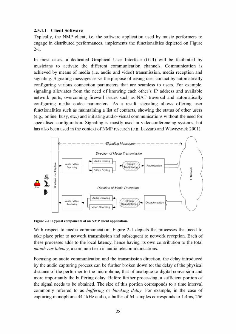
28
2.5.1.1 Client Software
Typically, the NMP client, i.e. the software application used by music performers to
engage in distributed performances, implements the functionalities depicted on Figure
2-1.
In most cases, a dedicated Graphical User Interface (GUI) will be facilitated by
musicians to activate the different communication channels. Communication is
achieved by means of media (i.e. audio and video) transmission, media reception and
signaling. Signaling messages serve the purpose of easing user contact by automatically
configuring various connection parameters that are seamless to users. For example,
signaling alleviates from the need of knowing each other’s IP address and available
network ports, overcoming firewall issues such as NAT traversal and automatically
configuring media codec parameters. As a result, signaling allows offering user
functionalities such as maintaining a list of contacts, showing the status of other users
(e.g., online, busy, etc.) and initiating audio-visual communications without the need for
specialised configuration. Signaling is mostly used in videoconferencing systems, but
has also been used in the context of NMP research (e.g. Lazzaro and Wawrzynek 2001).
Figure 2-1: Typical components of an NMP client application.
With respect to media communication, Figure 2-1 depicts the processes that need to
take place prior to network transmission and subsequent to network reception. Each of
these processes adds to the local latency, hence having its own contribution to the total
mouth-ear latency, a common term in audio telecommunications.
Focusing on audio communication and the transmission direction, the delay introduced
by the audio capturing process can be further broken down to: the delay of the physical
distance of the performer to the microphone, that of analogue to digital conversion and
more importantly the buffering delay. Before further processing, a sufficient portion of
the signal needs to be obtained. The size of this portion corresponds to a time interval
commonly referred to as buffering or blocking delay. For example, in the case of
capturing monophonic 44.1kHz audio, a buffer of 64 samples corresponds to 1.4ms, 256

29
samples correspond to 5.8ms and 1024 samples correspond to 23.2ms. Hence, the size
of the audio buffer should be appropriately eliminated to correspond to latencies that are
sufficiently lower than the EPT.
In some cases, audio capturing is followed by compression encoding. Audio
compression aims at reducing the size of the information to be transmitted, hence
eliminating the required network bandwidth. It is straightforward to estimate that raw
monophonic CD quality audio (44.1kHz/16bit) corresponds to a bit rate of 705.6kbps,
while the stereo signal requires 1.41Mbps. Clearly, requiring more audio channels or
higher quality audio in terms of sampling rate or bit resolution further increases the data
rate and hence the required network throughput.
These bitrates cannot be continuously available during NMP. Thus, some NMP
approaches employ compression encoding to reduce the required bandwidth (e.g.
Polycom 2011; Kurtisi and Wolf 2008; Kraemer et al. 2007). Nevertheless, some NMP
systems, and especially those intended for use over academic networks (Alexandraki
and Akoumianakis 2010; Cáceres and Chafe 2009; Sawchuck et al. 2003) do not use
audio compression. The choice of whether or not to use audio compression is primarily
determined by the latencies introduced by the compression codec. Encoding latencies
comprise both delays caused by the algorithmic complexity of the encoder as well as
buffering delays. Compression schemes conventionally require a sufficient amount of
data (hence increasing the buffer size), so as to effectively encode data streams and
offer commendable data reduction.
Further to compression encoding, an NMP client may optionally perform multiplexing.
Multiplexing serves the purpose of combining multiple data streams in one stream, so as
to eliminate the need for using an additional network port, hence a separate
configuration at the receiving end, for each individual stream. For example multiple
streams of audio or video could be combined in a single stream. Multiplexing is
generally a lightweight process that does not significantly add to the overall latency.
Finally, before departing to the network the possibly encoded and multiplexed audio
chucks are wrapped in network packets. Apart from the main data, i.e. the payload,
network packets include header information. Header information is determined and
structured according to network protocol facilitated for media transmission. Header
information is necessary and among other things defines the destination of each network
packet. The network protocols used by NMP applications are briefly discussed in
section 2.5.2.2. It is important to note that header information adds to the total data rate,
hence increasing the required network bandwidth. A research initiative attempting to
reduce header overhead in NMP is presented by Kurtisi and Wolf (2008).
It can be seen from Figure 2-1, that the inverse processes takes place in the direction of
media reception. Although processes such as audio decoding and audio rendering are
more lightweight than encoding or capturing, media reception is not necessarily more
efficient than media transmission. This is due to the fact that in the event of multiple
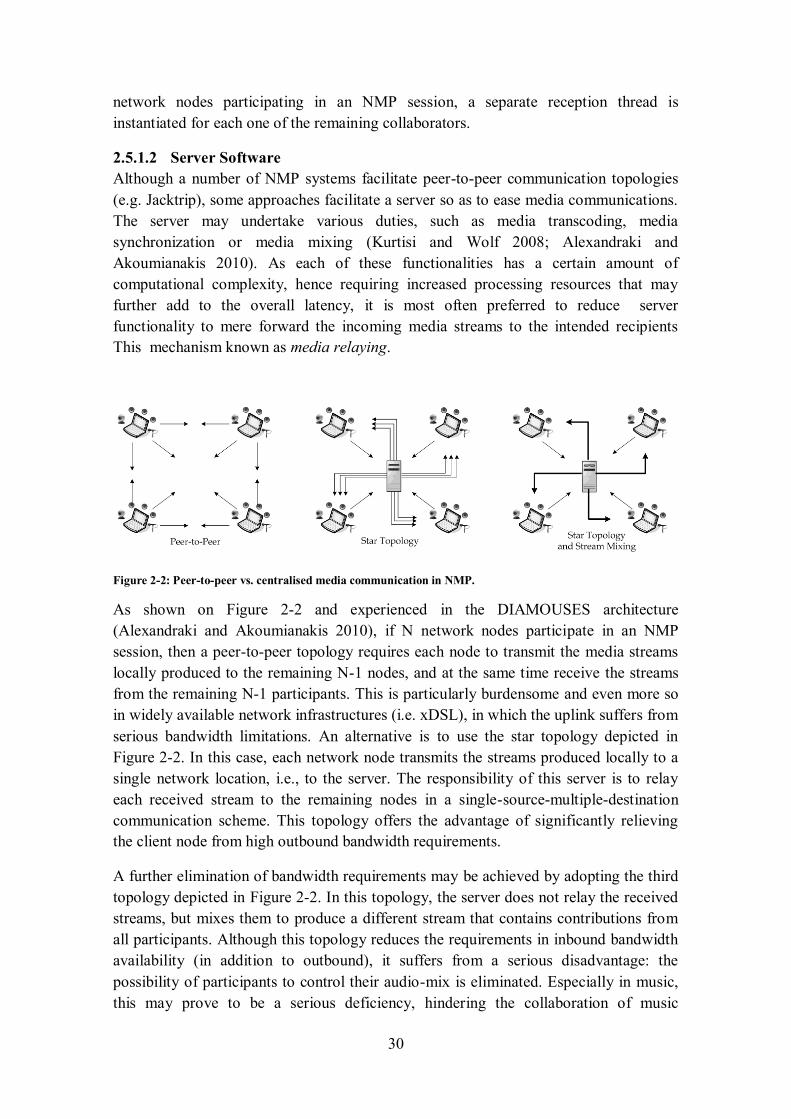
30
network nodes participating in an NMP session, a separate reception thread is
instantiated for each one of the remaining collaborators.
2.5.1.2 Server Software
Although a number of NMP systems facilitate peer-to-peer communication topologies
(e.g. Jacktrip), some approaches facilitate a server so as to ease media communications.
The server may undertake various duties, such as media transcoding, media
synchronization or media mixing (Kurtisi and Wolf 2008; Alexandraki and
Akoumianakis 2010). As each of these functionalities has a certain amount of
computational complexity, hence requiring increased processing resources that may
further add to the overall latency, it is most often preferred to reduce server
functionality to mere forward the incoming media streams to the intended recipients
This mechanism known as media relaying.
Figure 2-2: Peer-to-peer vs. centralised media communication in NMP.
As shown on Figure 2-2 and experienced in the DIAMOUSES architecture
(Alexandraki and Akoumianakis 2010), if N network nodes participate in an NMP
session, then a peer-to-peer topology requires each node to transmit the media streams
locally produced to the remaining N-1 nodes, and at the same time receive the streams
from the remaining N-1 participants. This is particularly burdensome and even more so
in widely available network infrastructures (i.e. xDSL), in which the uplink suffers from
serious bandwidth limitations. An alternative is to use the star topology depicted in
Figure 2-2. In this case, each network node transmits the streams produced locally to a
single network location, i.e., to the server. The responsibility of this server is to relay
each received stream to the remaining nodes in a single-source-multiple-destination
communication scheme. This topology offers the advantage of significantly relieving
the client node from high outbound bandwidth requirements.
A further elimination of bandwidth requirements may be achieved by adopting the third
topology depicted in Figure 2-2. In this topology, the server does not relay the received
streams, but mixes them to produce a different stream that contains contributions from
all participants. Although this topology reduces the requirements in inbound bandwidth
availability (in addition to outbound), it suffers from a serious disadvantage: the
possibility of participants to control their audio-mix is eliminated. Especially in music,
this may prove to be a serious deficiency, hindering the collaboration of music

31
performers. During live performances, musicians may need to occasionally increase the
audio level of certain ensemble members or even mute or solo the playback of one of
them. Evidently, the position of musicians in orchestral settings is deliberately such that
musicians collaborating more closely, e.g., woodwind, strings etc. are positioned closer
to each other. An alternative to providing a single mix to all participants, would be to
require that an audio mixing server provides a different mix for each participating
network node, which can controlled by that node. Unfortunately, this approach requires
a great amount of signal processing performed on the server, as all streams need to be
decoded, mixed or composited according to each participant’s requirements and then re-
encoded. This scheme not only requires considerable processing resources but also
introduces a considerable amount of delay. For all these reasons, it is generally more
efficient to adopt the solution depicted in the centre of Figure 2-2, which is for example
realized in the Ninjam framework5.
2.5.2 Network infrastructures
Besides software architectures, the prevalent problems of NMP are related to the actual
medium of communication, the network. The next section describes these problems in
more detail, while the section that follows gives a brief description of the network
protocols that are most commonly facilitated in NMP.
2.5.2.1 QoS issues
The term Quality of Service (QoS) is used to describe the means to prioritize network
traffic, so as to help ensure that the most important data gets through the network as
quickly as possible. To quantitatively measure QoS several related aspects of the
network service are often considered, such as error rates, network throughput,
transmission delay, jitter, etc. In the following, QoS is discussed in terms of bandwidth
availability, latency and jitter as well as packet loss.
2.5.2.1.1 Network throughput
Bandwidth availability or network throughput refers to the capacity of the network to
accommodate certain data rates. As already discussed, using raw CD quality audio
requires a continuous throughput of more than 1.41Mbps (as this value excludes header
overhead). Due to varying load from disparate users sharing the same network
resources, the bit rate that can be provided to a certain data stream may be too low for
real-time multimedia services if all data streams get the same scheduling priority. When
the load of the network is greater than its capacity can handle, the network becomes
congested. Characteristics of a congested network path are queuing delays, packet loss
and sometimes the blockage of new connections.
2.5.2.1.2 Latency and Jitter
Network latency refers to the time elapsed for a network packet to reach its intended
destination. In the widely used connectionless packet-switching network connections,
5 http://www.cockos.com/ninjam/
32
the routing path of a network packet is neither known beforehand nor can be controlled.
Depending on the actual transmission path, a packet may require a long time to reach its
destination, because it may be held up in long queues, or take a less direct route to avoid
congestion. This is different from throughput, as the delay can build up over time, even
if the throughput is almost normal. In some cases, excessive latency can render the
application unusable.
Measuring network latencies is not a trivial task especially due to synchronization
inaccuracies and clock drifts. Network latencies are often measured either as one way
packet delivery or as round trip delay times. One way latency refers to measuring the
time elapsed between sending a packet from one location and receiving it at a different
location. In this case, accurate measurements require synchronizing the clocks of the
transmitter and the receiver, which is a difficult task in its own behalf. Alternatively, the
parameter Round-Trip Time (RTT) refers to the time elapsed between sending a packet
to a remote location and receiving it back. In this case, time is measured from a single
point and the need for synchronization is eliminated. However, measuring the actual
transmission latency is still inaccurate, since the RTT values contain the time taken by
processing the packet at its destination and before sending back the response. The ping
utility offers a solution to this problem as it performs no packet processing at the the
receiving end. It merely sends a response back as soon as it receives an ICMP packet.
The Internet Control Messaging Protocol (ICMP) is the protocol used by the ping
utility. However, ICMP packets are normally given low priority by network devices
such as routers and switches. Hence, their delivery may be delayed by queuing them
between subsequent hops which does not commonly occur in the transmission of actual
TCP or UDP data packets. For this reason, RTT values reported by the ping utility
present a theoretical maximum in the delivery of actual TCP or UDP packets. The ping
utility is the most frequently method for measuring communication latencies in NMP
and has also been adopted in the evaluation of BoogieNet, the prototype system under
investigation (section 11.3.2).
Further to latency, a more important obstruction in NMP and teleconferencing
applications stems from the fact that the different network packets will reach their
destination with different delays. Variation in the delivery time of different packets is
known as network jitter or more formally Packet Delay Variation (PDV). PDV may be
due to queuing network packets on different network devices across the transmission
path, or due to packets being driven in different routing paths. Since media playback
requires a steady pace, PDV must be eliminated either in the network, or at the end host.
Playing the received packets at a steady pace can compensate for network PDV.
Reducing PDV in the network requires QoS guarantees and stable routes, which are
generally not feasible on the Internet on an end-to-end basis.
2.5.2.1.3 Packet Loss
Finally, packet loss occurs when one or more packets of data travelling across a
computer network fail to reach their destination. In Wide Area Networks packet loss is

33
frequently observed and caused by congested network paths or data corruption by faulty
networking hardware across the path. In the case of audio, losing network packets will
result in audio dropouts on the waveform rendered after de-packetisation and possible
de-multiplexing and decoding (see Figure 2-1). The distortion introduced by audio
dropouts can seriously hinder the collaboration of music performers.
Some network transport protocols, such as TCP, provide mechanisms for reliable
delivery of packets. In the event of a lost packet, the receiver asks for retransmission or
the sender automatically resends any segments that have not been acknowledged. This
method of error handling is known as Automatic Repeat reQuest (ARQ). Clearly, ARQ
is not an appropriate error correction method for real-time multimedia communications,
as in VoIP or NMP the packets received after retransmission will be outdated. This is
the main reason why, instead of TCP the more lightweight and less reliable UDP
transport protocol is preferred in applications involving real-time media
communications. Protocols such as UDP provide no mechanisms for recovering lost
packets. Applications that use UDP are expected to define their own mechanisms for
handling packet loss.
2.5.2.2 Network protocols
The User Datagram Protocol (UDP) is one of the core members of the Internet
Protocol suite (the set of network protocols used for the Internet). With UDP, computer
applications can send messages, in this case referred to as datagrams, to other hosts on
an Internet Protocol (IP) network without prior communications to set up special
transmission channels or data paths.
Figure 2-3: The format of the IP header. The numbers on top indicate the number of bits required for each
field. The fields appearing on the 6th
layer are optional.
In comparison to Transmission Control Protocol (TCP), UDP is a simpler message-
based connectionless protocol. Connectionless protocols do not set up a dedicated end-
to-end connection. Communication is achieved by transmitting information in one
direction from source to destination without verifying the readiness or state of the
receiver. Compared to TCP, UDP does not offer any mechanism for ensuring the
delivery of network packets to its intended recipient, which is why UDP is considered
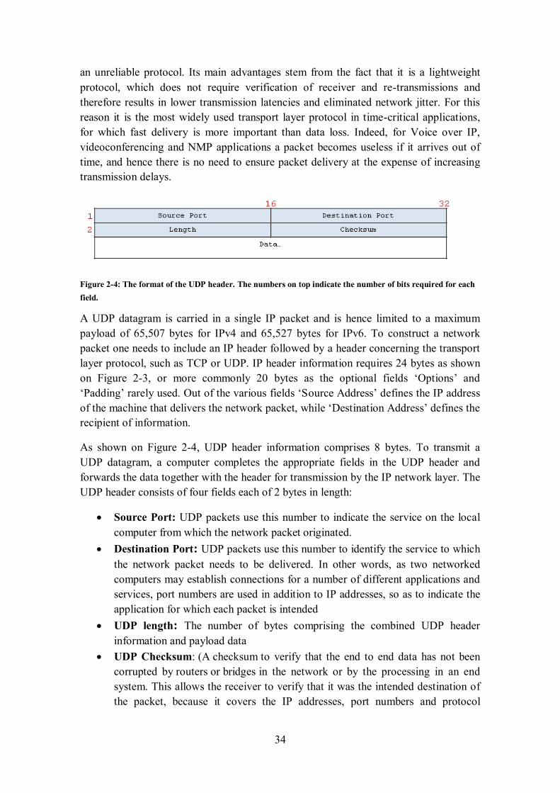
34
an unreliable protocol. Its main advantages stem from the fact that it is a lightweight
protocol, which does not require verification of receiver and re-transmissions and
therefore results in lower transmission latencies and eliminated network jitter. For this
reason it is the most widely used transport layer protocol in time-critical applications,
for which fast delivery is more important than data loss. Indeed, for Voice over IP,
videoconferencing and NMP applications a packet becomes useless if it arrives out of
time, and hence there is no need to ensure packet delivery at the expense of increasing
transmission delays.
Figure 2-4: The format of the UDP header. The numbers on top indicate the number of bits required for each
field.
A UDP datagram is carried in a single IP packet and is hence limited to a maximum
payload of 65,507 bytes for IPv4 and 65,527 bytes for IPv6. To construct a network
packet one needs to include an IP header followed by a header concerning the transport
layer protocol, such as TCP or UDP. IP header information requires 24 bytes as shown
on Figure 2-3, or more commonly 20 bytes as the optional fields ‘Options’ and
‘Padding’ rarely used. Out of the various fields ‘Source Address’ defines the IP address
of the machine that delivers the network packet, while ‘Destination Address’ defines the
recipient of information.
As shown on Figure 2-4, UDP header information comprises 8 bytes. To transmit a
UDP datagram, a computer completes the appropriate fields in the UDP header and
forwards the data together with the header for transmission by the IP network layer. The
UDP header consists of four fields each of 2 bytes in length:
Source Port: UDP packets use this number to indicate the service on the local
computer from which the network packet originated.
Destination Port: UDP packets use this number to identify the service to which
the network packet needs to be delivered. In other words, as two networked
computers may establish connections for a number of different applications and
services, port numbers are used in addition to IP addresses, so as to indicate the
application for which each packet is intended
UDP length: The number of bytes comprising the combined UDP header
information and payload data
UDP Checksum: (A checksum to verify that the end to end data has not been
corrupted by routers or bridges in the network or by the processing in an end
system. This allows the receiver to verify that it was the intended destination of
the packet, because it covers the IP addresses, port numbers and protocol
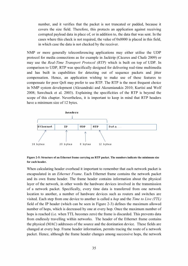
35
number, and it verifies that the packet is not truncated or padded, because it
covers the size field. Therefore, this protects an application against receiving
corrupted payload data in place of, or in addition to, the data that was sent. In the
cases where this check is not required, the value of 0x0000 is placed in this field,
in which case the data is not checked by the receiver.
NMP or more generally teleconferencing applications may either utilise the UDP
protocol for media connections as for example in Jacktrip (Cáceres and Chafe 2009) or
may use the Real-Time Transport Protocol (RTP) which is built on top of UDP. In
comparison to UDP, RTP was specifically designed for delivering real-time multimedia
and has built in capabilities for detecting out of sequence packets and jitter
compensation. Hence, an application wishing to make use of these features to
compensate for poor QoS may prefer to use RTP. The RTP is the most frequent choice
in NMP system development (Alexandraki and Akoumianakis 2010; Kurtisi and Wolf
2008; Sawchuck et al. 2003). Explaining the specificities of the RTP is beyond the
scope of this chapter. Nevertheless, it is important to keep in mind that RTP headers
have a minimum size of 12 bytes.
Figure 2-5: Structure of an Ethernet frame carrying an RTP packet. The numbers indicate the minimum size
for each header.
When calculating header overhead it important to remember that each network packet is
encapsulated in an Ethernet Frame. Each Ethernet frame contains the network packet
and its own frame header. The frame header contains information about the physical
layer of the network, in other words the hardware devices involved in the transmission
of a network packet. Specifically, every time data is transferred from one network
location to another, a number of hardware devices such as routers and switches are
visited. Each step from one device to another is called a hop and the Time to Live (TTL)
field of the IP header (which can be seen in Figure 2-3) defines the maximum allowed
number of hops, which is decreased by one at every hop. Once the maximum number of
hops is reached (i.e. when TTL becomes zero) the frame is discarded. This prevents data
from endlessly travelling within networks. The header of the Ethernet frame contains
the physical (MAC) addresses of the source and the destination device. These fields are
changed at every hop. Frame header information, permits tracing the route of a network
packet. Hence, although the frame header changes among successive hops, the network
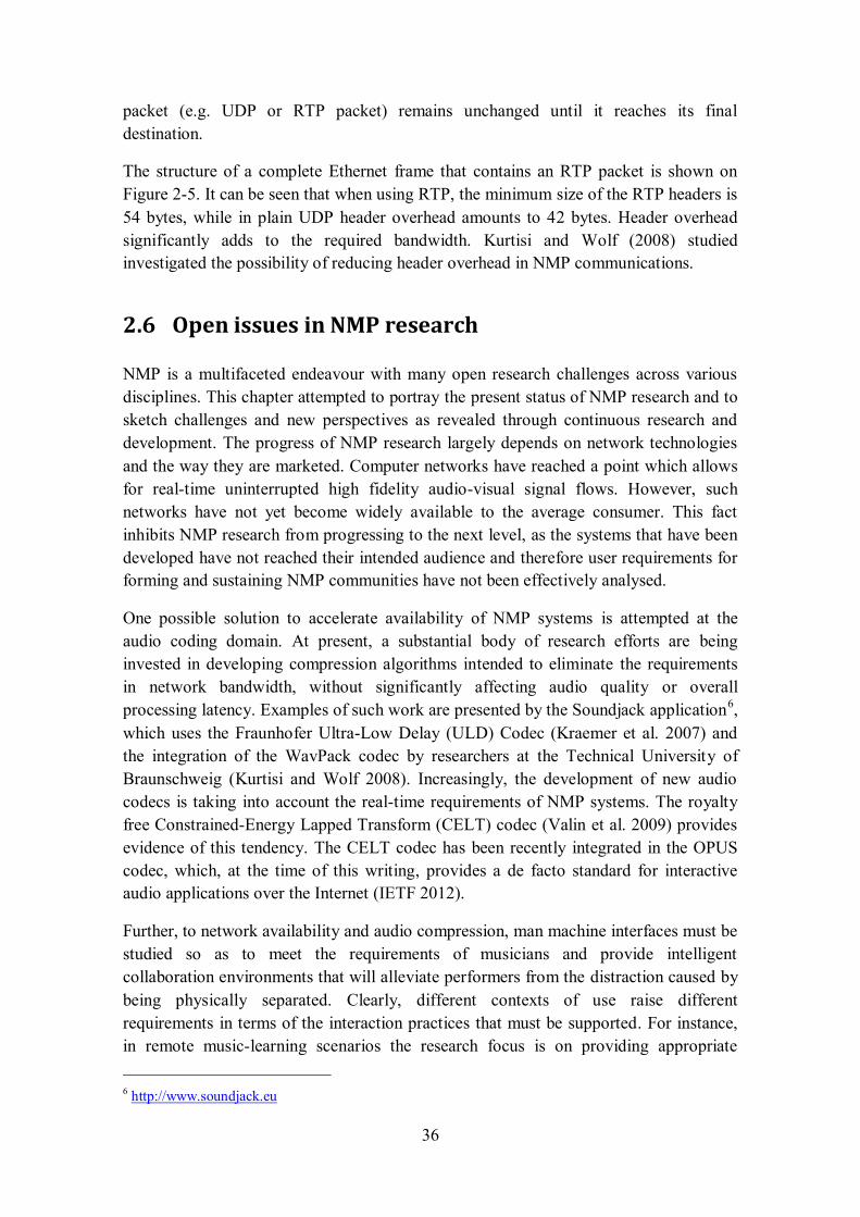
36
packet (e.g. UDP or RTP packet) remains unchanged until it reaches its final
destination.
The structure of a complete Ethernet frame that contains an RTP packet is shown on
Figure 2-5. It can be seen that when using RTP, the minimum size of the RTP headers is
54 bytes, while in plain UDP header overhead amounts to 42 bytes. Header overhead
significantly adds to the required bandwidth. Kurtisi and Wolf (2008) studied
investigated the possibility of reducing header overhead in NMP communications.
2.6 Open issues in NMP research
NMP is a multifaceted endeavour with many open research challenges across various
disciplines. This chapter attempted to portray the present status of NMP research and to
sketch challenges and new perspectives as revealed through continuous research and
development. The progress of NMP research largely depends on network technologies
and the way they are marketed. Computer networks have reached a point which allows
for real-time uninterrupted high fidelity audio-visual signal flows. However, such
networks have not yet become widely available to the average consumer. This fact
inhibits NMP research from progressing to the next level, as the systems that have been
developed have not reached their intended audience and therefore user requirements for
forming and sustaining NMP communities have not been effectively analysed.
One possible solution to accelerate availability of NMP systems is attempted at the
audio coding domain. At present, a substantial body of research efforts are being
invested in developing compression algorithms intended to eliminate the requirements
in network bandwidth, without significantly affecting audio quality or overall
processing latency. Examples of such work are presented by the Soundjack application6,
which uses the Fraunhofer Ultra-Low Delay (ULD) Codec (Kraemer et al. 2007) and
the integration of the WavPack codec by researchers at the Technical University of
Braunschweig (Kurtisi and Wolf 2008). Increasingly, the development of new audio
codecs is taking into account the real-time requirements of NMP systems. The royalty
free Constrained-Energy Lapped Transform (CELT) codec (Valin et al. 2009) provides
evidence of this tendency. The CELT codec has been recently integrated in the OPUS
codec, which, at the time of this writing, provides a de facto standard for interactive
audio applications over the Internet (IETF 2012).
Further, to network availability and audio compression, man machine interfaces must be
studied so as to meet the requirements of musicians and provide intelligent
collaboration environments that will alleviate performers from the distraction caused by
being physically separated. Clearly, different contexts of use raise different
requirements in terms of the interaction practices that must be supported. For instance,
in remote music-learning scenarios the research focus is on providing appropriate
6 http://www.soundjack.eu
37
pedagogical paradigms and on exploring methods for the evaluation of student progress
(Ng and Nesi 2008). Furthermore, in collaborative music composition (Hajdu 2005), a
key challenge relates to representing musical events effectively and devising appropriate
musical notations (Hajdu 2006). In the context of the DIAMOUSES framework
(Alexandraki and Akoumianakis 2010) research investigations focused on
accommodating diverse user requirements in music performance across different
collaboration scenarios such as rehearsals, stage performances and music lessons.
Graphical User Interfaces such as the one depicted in Figure 2-6 present innovative
approaches in dealing with collaboration deficiencies (see section 2.2). Such interfaces
integrate the audiovisual communication of musicians with shared collaborative objects
(e.g. a shared music score or metronome) that allow synchronous manipulations
accessible to all participants, hence maintaining a sense of user focus and promoting a
collaborative perspective. Computer Supported Collaborative Work (CSCW) is a focal
point of research for several application domains, including e-gaming, e-learning and
enterprise groupware, to name a few. The limited availability of reliable NMP systems
does not provide sufficient motivation for instantiating CSCW research in distributed
music performances.
Figure 2-6: A GUI offering virtual collaboration capabilities in NMP.
In the light of the above, a significant contribution to easing performers’ collaboration
across distance can be made through the development intelligent user interfaces that are
capable of extracting musically meaningful information from the audio signals
38
generated and exchanged in the course of a distributed performance. For example, the
‘performance worm’ devised by Langer and Goebl (2003) provides a visualization of
live performances, represented as the trajectory of a point on a two dimensional plane
depicting loudness versus tempo. The depicted trajectories are automatically derived
from audio analysis. Such real-time visualisations of the expressive performance can
create performance anticipations that may greatly enhance the collaboration of
musicians, for example in the presence of high communication delays or in the absence
of adequate visual contact.
Alternative possibilities may be devised by examining different collaboration scenarios
and contexts of use. Ultimately, incremental progress on machine listening systems and
computational music performance can directly translate to intelligent interfaces for
NMP. As further discussed in the next chapter, functionalities such as automatic music
transcription, automatic score scrolling and computer accompaniment may reveal their
full potential in the context of remote musical collaborations.

39
3 Machine Musicianship
Machine listening refers to the computational understanding of sounds (including
music, speech as well as environmental sounds) at a comparable level to the sound
understanding occurring in humans. In comparison, Machine musicianship focuses on
musical sounds, assumes musical machine listening capabilities and addresses
supplementary musical skills such as performance and composition. In line with human
musicianship, these skills require knowledge of musical concepts, which may be
inherent, learnt or developed through practice.
This chapter presents the overall research directions and perspectives in two areas.
Specifically, the first section discusses the general algorithmic processes taking place in
machine listening systems, while the second section presents previous and state-of-the-
art research achievements in machine musicianship for different musical skills which
are: music transcription, score following, audio synchronisation and computer
accompaniment. Finally, the third section attempts to track down research initiatives
that are relevant to the present work, hence investigating machine musicianship in
distributed performance context.
3.1 Machine Listening Approaches
Machine listening research deals with the computational modelling of sound
understanding. The objective of this area is to implement systems that are capable of
generating meaning in response to sound input, similarly to the cognitive understanding
of sound carried out by human listeners. In attempt to further refine the notion of
meaning, media theorist Hansen (2006) elucidates that the human body acts as a central
point for various sensory modalities. It essentially selects and subtracts from the totality
of images available and it is this act of subtraction and selection which is a meaning-
giving act that ‘in-forms’ our perception of information.
Equivalently, digital media represent the sensory stimuli of models of computational
intelligence, and indeed there is strong evidence in a plethora of information domains,
including music (Toiviainen et al. 1998; Bharucha & Todd 1989), that these models are
successful in deriving perceptually meaningful information. However, although
meaning-giving in computer intelligence may be successfully modelled, this does not
mean that the mechanisms employed by humans are similar to the algorithms employed
in computational intelligence. For example, although Artificial Neural Networks are
inspired from biological neurons, their biological counterparts are significantly more
complex. In a similar line, Hidden Markov Models use observation and transition
probabilities to perform abstraction of digital stimuli; nevertheless, it is not clear
40
whether similar processes occur in humans whose perception and cognition is strongly
influenced by complex psychological, physiological and neurological processes.
To this end, two distinct trends may be identified in machine listening research. The
first relates to initiatives developing computer models that simulate certain
characteristics of auditory perception (e.g. tonal or harmonic expectancies, judging
timbral similarities etc.) with the aim of understanding musical perception and
cognition, while the second relates to developing systems that extract perceptually
meaningful information for further use. Although the ultimate objective is common in
the two perspectives (i.e. to enable computers manipulate sound at a comparable level to
humans), however the adopted methodologies are profoundly different.
Computational simulations of the auditory perception commonly entail dynamic models
that describe perception as adaptation and synchronization, where sometimes only one
step is needed from a low-level to high-level feature estimations. Examples are neural
networks, both of the connectionist side of the perceptron model (e.g. Bharucha &Todd
1989; Gjerdingen 1990) and the Kohonen map side (e.g. Leman & Carreras 1997;
Toiviainen 1998; Kostek 2005) of self-organizing maps, modelling tonality, musical
phrases, or timbre perception. A similar idea about modelling memory in music that of
an echoic short-term memory, where a perceptual input is echoing in the brain, like an
impulse echoes in a concert hall, modelling short-time memory (Snyer 2000). This is
similar to the perceptron model, as in both an input echoes through the model until it
has decayed. A relatively new approach is the free-energy principle (Friston 2010;
Friston et al. 2010) which is a self-organizing perception model based on the principle
of minimizing surprise when adapting an internal state to a perception, taking memory
and also motion into consideration.
On the other hand, the development of computational models that aim at extracting
perceptually meaningful information from audio signals adopts a fairly application
oriented bottom-up approach, in which data reduction occurs in successive steps thereby
reducing the dimensionality of sound to higher level constructs. Such systems are said
to perform Computational Auditory Scene Analysis (CASA), a roughly coincident area
of research that aims at identifying the various sound events contained in a mixture of
sounds. Challenges arise when these events are simultaneous, masked by other sounds
or highly distorted.
According to Wang (2007), in humans scene analysis entails two basic perceptual
processes: the segmentation of a scene into a set of coherent patterns (objects) and the
recognition of memorized ones. Following, in the same article Wang states:
Human intelligence can be broadly divided into three aspects: Perception, reasoning, and
action. The first is mainly concerned with analyzing the information in the environment
gathered by the five senses, and the last is primarily concerned with acting on the
environment. In other words, perception and action are about input and output,
respectively, from the viewpoint of the intelligent agent (i.e. a human being). Reasoning
involves higher cognitive functions such as memory, planning, language understanding,
41
and decision making, and is at the core of traditional artificial intelligence. Reasoning also
serves to connect perception and action, and the three aspects interact with one another to
form the whole of intelligence.
In line with Wang’s comprehension of human intelligence, machine listening systems
manifest their intelligence in three sequential processes, namely:
Perception: Detection of sound objects by segmenting an auditory scene into its
constituent events based on the variation of a number of perceptually relevant
acoustic features
Reasoning: Identification of the context of one or more sound objects by
recognising patterns that have been registered and memorised in the course of
prior initialisation or training
Action: deliver custom functionalities based on the identified patterns
The content of sound to be processed in machine listening systems commonly falls in
one of the three categories, namely speech, environmental sound and music or
combinations of these. As depicted in Figure 3-1, although for different domains the
structural components of sound differ, the methodology for reducing the dimensionality
of an input signal to acquiring information that is semantically meaningful for the
application at hand is fundamentally the same. Starting from an audio signal, feature
extraction takes place so as to compute a number of acoustically relevant properties
corresponding to a small frame of audio. Following feature extraction, individual sound
events carrying structural information of interest are detected through a process called
temporal segmentation. Temporal segmentation concerns the detection of the
boundaries of sound events (i.e. onset and end-times) using the temporal behaviour of
acoustic features. These features must be carefully selected in order to efficiently reveal
segment boundaries. For example a sudden elevation of noise levels is typically caused
by a mechanical excitation and is often followed by a stationary sound event.
Consequently, acoustic features representing noisy components in the signal are highly
appropriate for detecting the onsets of sound events.
Once sound events have been detected their frequency or timing of occurrence is used
by pattern recognition methodologies to convey their context. Such contextual
information characterises the information content carried by longer signal portions
(compared to audio segments) or the audio signal in its entity. Depending on the target
application, different levels of information content are used to determine or initiate
system actions. Some applications use the output of pattern recognition to offer user
functionalities while others, especially those requiring action that is constraint within
time limits, use directly the output of the temporal segmentation process. The following
paragraphs elaborate further on these processes and how they are realised for different
audio domains.
Most feature extraction schemes rely on a frame-based analysis, where overlapping
audio frames of 10–100 ms are windowed and used as the input for feature extraction.
In such short frames, dynamic audio sources tend to be stationary therefore allowing to
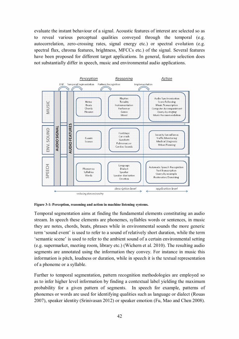
42
evaluate the instant behaviour of a signal. Acoustic features of interest are selected so as
to reveal various perceptual qualities conveyed through the temporal (e.g.
autocorrelation, zero-crossing rates, signal energy etc.) or spectral evolution (e.g.
spectral flux, chroma features, brightness, MFCCs etc.) of the signal. Several features
have been proposed for different target applications. In general, feature selection does
not substantially differ in speech, music and environmental audio applications.
Figure 3-1: Perception, reasoning and action in machine listening systems.
Temporal segmentation aims at finding the fundamental elements constituting an audio
stream. In speech these elements are phonemes, syllables words or sentences, in music
they are notes, chords, beats, phrases while in environmental sounds the more generic
term ‘sound event’ is used to refer to a sound of relatively short duration, while the term
‘semantic scene’ is used to refer to the ambient sound of a certain environmental setting
(e.g. supermarket, meeting room, library etc.) (Wichern et al. 2010). The resulting audio
segments are annotated using the information they convey. For instance in music this
information is pitch, loudness or duration, while in speech it is the textual representation
of a phoneme or a syllable.
Further to temporal segmentation, pattern recognition methodologies are employed so
as to infer higher level information by finding a contextual label yielding the maximum
probability for a given pattern of segments. In speech for example, patterns of
phonemes or words are used for identifying qualities such as language or dialect (Rouas
2007), speaker identity (Srinivasan 2012) or speaker emotion (Fu, Mao and Chen 2008).
43
In environmental sounds sequences of sound events are used to determine the presence
of certain types of human or other activity such as footsteps (Radhakrishnan, Divakaran
and Smaragdis 2005), car collisions, gun shots (Cai et al. 2006) or heart and lung
sounds (Yadollahi and Moussavi 2006) for medical applications. In the music domain,
pattern recognition applied on note, beat or phrase sequences leads to the identification
of contextual properties such as rhythmic structures (Goto 2001a), instrumentation
(Tetsuro et al. 2005), genre (Silla Koerich and Kaestner 2008) or mood (Oliveira and
Cardoso 2010) for a given piece of music.
Finally at the application level, Figure 3-1 shows potential functionalities offered by
systems receiving and analysing auditory input. In speech listening, prominent
functionalities are automatic speech recognition (Scharenborg 2007) and speech
restoration from noisy, reversed or corrupted sources (Srinivasan and Wang 2005). In
environmental audio, popular application domains include security surveillance (Harma,
Mc inney and Skowronek 2005), traffic monitoring (Fagerlönn and Alm 2010),
medical applications (Yadollahi and Moussavi 2006) and urban planning (Hedfors et al.
1998.). Generally, environmental auditory scene analysis is commonly used in
situations where visual information is either costly (e.g. inside the human body), limited
(e.g. dark places) or too broad (e.g. countryside), or alternatively in multimodal systems
in which monitoring and analysing the auditory information channel complements the
visual or some other sensory channel (Sanderson et al. 2004).
3.2 Music listening and relevant computational affordances
In the music domain, machine listening functionalities are similar to those addressed by
content-based music information retrieval. Content-based MIR approaches focus on
analysing music sources, which may be either music signals or symbolic representations
(MIDI, score etc.), so as derive music semantics characterising these sources (Casey et
al. 2008). The connotation ‘content-based’ is facilitated so as to distinguish from
‘context-based’ MIR approaches, in which musical metadata, such as lyrics, artists’
cultural background, band biographies etc., useful for indexing music, are derived by
employing Natural Language Processing (NLP) techniques on web-mined resources
(Schedl et al., 2011).
According to Rowe (2001), the term musicianship refers to the collective intelligence
relating to musical concepts that underlie the skills of listening (analysis), performance
and composition. Subsequently, machine musicianship refers to computational
programs designed to implement any of these skills. Relevant affordances of machine
musicianship systems that are potentially useful in distributed performance settings
include:
Automatic Music Transcription
Audio-to-score alignment
44
Audio-to-audio alignment
Computer Accompaniment
The following subsections discuss applications, challenges and methodologies related to
these capabilities and elaborate on previous and state-of-the-art research initiatives and
computational approaches.
3.2.1 Automatic music transcription
Automatic Music Transcription (AMT) refers to the possibility of generating a music
score given an audio signal. A music score, whether using the notation of the Western
music tradition or some other notation such as chord symbols, piano rolls or tablatures,
should, as a basic requirement, define the pitch, the timing and the musical instrument
for each music event in a piece of music. In comparison with humans, AMT systems are
required to perform equally or better than a well-trained and gifted musician. This is
made apparent if we consider that when listening to a piece of music, we can perceive
the melodic line, tap or sing along, recognise long-term structural parts such as chorus
and verse but more precise information such as timing of notes, harmonic changes and
detailed description of all concurrent melodic lines is less consciously perceived. As
generating a complete transcription of a music piece can be an extremely challenging
task, often impossible to achieve and especially in cases of polyphonic and poly-
instrumental music recordings, the objective of these systems is commonly constrained
in finding as many musical events as possible (complete transcription) or finding the
most dominant part of the sound such as the drum strokes or the bass-line (partial
transcription). An elaborate account of AMT approaches may be found in (Klapuri and
Davy 2006).
Regardless the approach, an AMT system is required to detect pitch, relative loudness
and timbre of sound events. Clearly, all of these attributes are related to human
perception and the correspondences with their physical counterparts (i.e. sound) are not
straightforward. Generally, the mapping of physical stimuli to psychological percepts,
since Fechner (1860), is called psychophysics and in terms of audition, psychoacoustics.
This mapping is not at all trivial. The psychological perception of pitch corresponds to
multiple acoustic features, most prominent the frequency presented, but also the
amplitude of this frequency. These two physical dimensions, frequency and amplitude,
are independent or orthogonal one to another on the physics side. Still they are no
longer independent in perception, where an increase of the amplitude of a sine wave
with a constant frequency leads to a perception of an increasing pitch (for a general
description and model see Garner 1974). Such phenomena are found nearly everywhere
in music perception, with pitch, timbre, rhythm, etc. Additionally, perception can also
be ambiguous, depending on listeners. As an example of pitch perception, Goldstein
proposed a statistical model of pitch perception, based on the harmonic overtone
content, amplitude, and slight frequency deviations (Goldstein 1973). Still pitch
perception may be simplified, as listeners tend to correct pitches which are deviating

45
from a ‘perfect’ pitch by categorizing tones into pitch classes, such as the twelve semi-
tones of an octave in Western music. So in AMT, to identify the pitch class does not
necessarily require to get into the details of pitch perception when it comes to
transforming the sound to a MIDI representation. Still, polyphonic texture instruments
or the singing voice tend to perform simple interval ratios using free intonation, in
which case it may be important to detect the precise pitch. Timbre on the other hand is
more difficult to model, as there is no single leading feature to account for the
instrument producing the sound. Timbre therefore is often found to be multi-
dimensional (Grey 1977; Bader 2013a), thus represented as vectors of acoustic features.
In addition to pitch and timbre, an AMT system is expected to account for the rhythmic
properties of a music piece, as these are depicted by the relative duration of note events.
In fact, instead of note durations, rhythm detection uses the variation of the Inter-Onset
Intervals (IOI) defined as the time intervals between the beginnings of two successive
notes (Goto 2001a). Although important for music transcription, note duration itself
does not always provide valuable indicator to rhythm detection. This is because in
percussive sounds with fast exponentially decaying envelopes, note durations are not
uniquely defined and in non-percussive sounds durations may be altered due to
performance articulation, for example in using legato and staccato notes. Evidently,
onset detection and therefore the accurate computation of IOIs can be a complicated
task by itself (Bello et al. 2005).
AMT has been the subject of several PhD theses since the seventies. The earliest
systematic attempt for the development of an AMT system is found in James Moorer’s
PhD thesis (1975). Moorer dealt with polyphony of two voices whose harmonic
relations were constrained to non-overlapping overtones, therefore disallowing unisons,
octaves, twelfths and some other intervals for which disambiguation of the two voices
would be significantly obscured. Following, the works of Pisczcalski and Geller (1977)
and Chafe et al. (1982) proposed certain improvements, however still limiting the
musical material to two-voice polyphony. Notably, in the first of these works
computational intelligence was employed to statistically infer the musical notes that
could best account for the observed frequency amplitude and time variations. Later in
1985, Schloss in his PhD thesis (Schloss 1985) focused on percussive musical
instruments and was therefore oriented towards the identification of rhythmic patterns.
Finally, Anssi lapuri’s PhD (2004) dealt with polyphonic music including but not
constraint in percussive sounds. Moreover, lapuri’s work considered musical meter
estimation and proposed certain techniques for the subtasks of multiple f0 estimation
(i.e. pitch of simultaneous notes) and onset detection.
Current AMS systems offer various improvements, however still suffering from several
limitations. In particular, significant accuracy has been achieved in the transcription of
either percussive or pitched instruments for recordings comprising of a limited number
of instruments (Davy and Godsill 2002; Tolonel and Karjalainen 2000) or for a single
instrument (Raphael 2002). More promising works dealing with more generic, less
46
constrained musical signals are those of Ryynänen and lapuri (2008) and Goto
(2001b). In fact, Goto (2001b) presents a system for transcribing the melody and
baseline of an unconstraint CD recording in real-time. Finally, another attempt for real-
time music transcription is presented in (Dessein, Cont and Lemaitre 2010), where
transcription is carried out for a live piano performance.
Score transcription often employs computational methods that are not instrument
specific, thereby disregarding the fact that different timbral characteristics may not be
captured equally well by a single computational model (Benetos et al. 2012).
Configuring these models for specific instruments requires that the instrument is known
or identifiable from the audio signal. Identifying instruments in poly-phonic and poly-
instrumental recordings is a particularly cumbersome task, related to sound source
separation. To this end Eggink and Brown (2003) proposed generating time-frequency
masks that isolate the spectral regions of specific instruments which can then be
classified more accurately.
An implementation of AMT is not attempted in current work. However, the continuous
evolution of techniques towards robust music transcription can provide a significant
improvement in the collaboration of dislocated music performers.
3.2.2 Audio-to-score alignment
Audio-to-score alignment seeks to find correspondences between a symbolic music
representation and an audio performance of the same piece of music. There are two
different approaches of the same problem, namely offline audio-to-score alignment,
often referred to as score matching and online audio-to-score alignment, often referred
to as score following or score scrolling.
In offline settings, both score and audio representations are available prior to matching.
Hence the matching algorithm is able to search the entire waveform in order to match
each score event. There are several applications sought by score matching, such as
easing digital audio editing and post-processing that often requires knowledge of the
location of a particular note or phrase in the score (Liu, Dannenberg and Cai 2010),
allowing automatic annotation in music libraries for search and retrieval (Miotto and
Lanckriet, 2012), or more generally providing automatic audio segmentations
(Dannenberg 2006), a task that is a prerequisite to most applications of machine
musicianship.
Online or real-time audio-to-score alignment assumes the score is available prior to
matching but the audio signal is progressively acquired. Thus, at any time only past and
present knowledge about the signal is available and the goal is to identify the musical
events depicted on the score as soon as they appear on the audio waveform, with high
temporal accuracy and within the minimum possible latency. Mainly, two applications
are sought in this context: aiding musicians with enhanced score visualizations such as
47
page turners (Arzt, Widmer and Dixon 2008; Dannenbeg et al. 1993) and live computer
accompaniment (Raphael 2001; Dannenberg and Raphael 2006).
The most popular computational techniques employed in audio-to-score alignment are
Dynamic Time Warping (DTW), Hidden Markov Models (HMM) and more recently
Particle Filters. Each approach is briefly described in the following paragraphs:
DTW was originally applied to identify speech patterns in speech recognition (Rabiner
and Juang 1993). It is a consolidated technique that finds the best match between two
sequences according to a number of constraints. Typically (Müller 2010), these
constraints concern boundary conditions (i.e. both sequences are bounded and assumed
to match both at their starting and at their ending point), a monotonicity condition
(requiring that the matching path progresses in the same direction i.e. it does not move
back and forth) and a step wise condition (requiring continuity of the matching path i.e.
no jumps). DTW has been extensively used for offline audio matching (Hu, Dannenberg
and Tzanetakis 2003; Soulez, Rodet, Schwarz 2003; Orio and Scwarz 2001). Generally
DTW is highly robust in offline settings but it is very inaccurate in real-time settings.
Online variants of the DTW algorithm have been sporadically presented in the relevant
literature (Dixon 2005; Marcae and Dixon 2010a). However, these variants are applied
in audio-to-audio synchronisation instead of score following. Even in the work of
Marcae and Dixon (2010b), where the ultimate goal is to provide score following, this is
achieved by synchronising the real-time waveform with an alternative audio signal
which has been synthesized from MIDI and is therefore an audio-to-audio alignment
task.
HMMs, although generally less accurate than DTW approaches, are more appropriate
for real-time alignments. HMMs are probably the most widely used technique in audio-
to-score alignment (both offline and online) and is the one used in the prototype system
developed in this work. An elaborate description of HMM mathematical foundations
and their use for audio-to-score alignment is provided in a Chapter 8. One of the main
issues concerning HMM score following is the fact that the Markovian model used for
alignment is associated with various probability values, which must be estimated prior
to alignment, during an offline process called training. HMMs may be trained using a
pre-existing manual alignment of a score to an audio file (i.e. supervised learning),
without any pre-existing alignment (i.e. using techniques of unsupervised learning)
(Raphael 1999) or using discriminative training, namely estimating an approximate
alignment and then further improving it using some training technique. Approximate
alignments may for example be estimated from an offline DTW alignment or blindly
from feature values. For example in (Cont 2004) the YIN pitch detection algorithm (de
Cheveigné and Kawahara 2002) is used to estimate the occurrence of notes on the audio
waveform. HMM probabilities are initially estimated according the produced alignment
and further refined by an iterative training process prior to using the model for real-time
alignment. Yet, more recent works of Cont (2010) present an HMM alignment system
that does not require any prior training. It uses a hybrid Markov/Semi Markov Model
48
which deals explicitly with tempo estimation and does not require any training of HMM
probabilities.
A further computational technique employed in audio-to-score alignment, is presented
by Particle Filter approaches. Particle filters do not require any training and are
remarkably appropriate for real-time alignments. Particle filters, also known as
Sequential Monte Carlo methods, operate by recursively approximating the alignment
of two sequences assumed to have a Markovian state evolution (i.e. the current state
depends only on the previous state and the current observation). In the context of
statistical models such as HMM and Particle filters, ‘filtering’ refers to determining the
distribution of a latent variable (i.e. score position) at a specific time (i.e. on the audio
signal), given all observations up to that time. An explanation of the theory of Particle
Filters is beyond the scope of this dissertation and it can be found in dedicated tutorials
(e.g. Arulampalam, Maskell and Gordon 2002). Particle filters have been recently used
for score following (Montecchio and Cont 2011a; Duan and Pardo 2011a) as well as for
real-time robotic performance enabled by means of score following (Otsuka et al. 2011).
3.2.3 Audio-to-audio alignment
Audio-to-audio alignment or audio synchronization aims at temporally aligning two
waveforms representing different interpretations of the same piece of music. Audio
synchronization has received less attention than audio-to-score alignment. However,
from a user oriented perspective, this task can also offer several practical applications.
The prevalent application of this task relates to the possibility of comparing different
interpretations of the same piece of music. Such comparison may be useful in the
context of computational musicology, for example by investigating expressive aspects
of music performances or the individualities of the performance by different artists.
Audio synchronization meets its full potential in digital music libraries offering efficient
browsing and random access within music recordings. A further application of audio
synchronization is additionally presented in the domain of studio engineering, for
example by allowing to time align different recording takes of a reference performance
during digital mixing (Montecchio and Cont 2011b).
In respect with the adopted computational techniques, most approaches use DTW, while
some more recent works have attempted audio synchronization using particle filters.
HMMs are not an appropriate strategy for directly aligning audio streams. As will be
seen in Chapter 8, HMMs aim at finding a sequence of hidden variables from within a
sequence of observable variables. In such cases as in audio-to-score alignment
observable variables are represented as sequences of feature vectors and hidden
variables are represented by higher –level and information of lower dimension such as
notes or chords. In audio-to-audio alignment, such higher–level representation is neither
available nor needs to be identified. The following paragraphs provide some
representative initiatives in this research track.
49
Match (Dixon and Widmer 2005), is a freely available software program for audio to
audio alignment developed in Java. It is based on an efficient DTW algorithm which has
time and space costs that are linear with respect to the length of the performances to be
aligned. The audio data is represented by positive spectral difference vectors. Frames of
audio input are converted to a frequency domain representation using a Short Time
Fourier Transform, and then mapped to a non-linear frequency scale, which is linear at
low frequencies and logarithmic at high frequencies. The time derivative of this
spectrum is then half-wave rectified and the resulting vector is used in the dynamic time
warping algorithm’s cost function, using a Euclidean metric.
In a similar line, Muller, Mattes and Kurth (2006), propose an alternative variant of
DTW, called Multi-Scale-DTW. They use an overlap-add technique based on waveform
similarity (WSOLA) to produce a stereo file in which the left channel carries one of the
recordings to be aligned and the right channel contains a time-warped version of the
second recording, using the results of their DTW algorithm. In a more recent work
Muller and Appelt (2008), aimed at synchronizing recordings having significant
structural differences such as omissions of repetitions, insertion of additional parts (soli,
cadenzas), or differences in the number of stanzas in popular, folk, or art songs.
Typically, DTW requires the complete series of both input streams in advance and has
quadratic time requirements. As such, DTW is unsuitable for real-time applications and
is inefficient for aligning long sequences. Nevertheless, Marcae and Dixon (2010)
presented a real-time variant of the DTW. Unfortunately, they used a hop size of 50ms
or more to derive their chroma features used for calculating sequence similarities. As a
result, time precision may not be sufficient for real-time applications.
Recent works on audio synchronization using particle filter approaches (Xion and
Izmirli 2012; Montecchio and Cont 2011a) seem to advance the development of real-
time synchronization. For instance the present work, as well as most research initiatives
in computer-based musical accompaniment could benefit from aligning the live audio
stream with a reference recording instead of requiring the presence of the score, which
is undoubtedly less informative in terms of tempo variability and expressive
articulations.
3.2.4 Computer accompaniment and robotic performance
Computer accompaniment aims at the development of techniques that allow a computer
system to listen to a live performer and synchronously reproduce an existing
accompaniment.
In line with the Turing test7, Barry Vercoe (1984) defines this objective as:
7 The Turing test is a test of a machine's ability to exhibit intelligent behaviour equivalent to, or
indistinguishable from that of an actual human. It involves a human judge who engages in a natural

50
to understand the dynamics of live ensemble performance well enough to
replace any member of the group by a synthetic performer (i.e. a computer
model) so that the remaining live members cannot tell the difference.
That same work reports on an accompaniment system which follows the live
performance of a flutist. Tracking the live performance was achieved using pitch
detection assisted by fingering information captured by optical sensors and score
information. Finally, the synthetic sound was generated using the 4X real-time audio
processor of that time. In the same article, Vercoe further reports on his intensions to
incorporate learning strategies so that the synthetic performer can progressively improve
from past experiences.
At the same time, Dannenberg (1984) presents an implementation of matching a live
monophonic keyboard performance to a score using dynamic programming techniques
inspired from string matching. His algorithm of note matching allows ignoring wrong
notes played by the performer. Output is synthesized using conventional digital
synthesizers of that time. Later, Bloch and Dannenberg (1985) attempted to extend their
system to polyphonic keyboard matching, while Vercoe and Puckette (1985) employed
an offline training method using data from past rehearsals, so as to allow the
anticipation of certain tempo deviations from the predefined score tempo.
In the years that followed, most research efforts concentrated in audio-to-score
alignment of monophonic (Raphael 1999) and polyphonic music (Raphael 2004),
without however abandoning the ultimate goal which was to develop real-time
computer-based performers. In 2001, Raphael presents his Music-Plus-One8 system
(Raphael 2001a) for the first time. Music-Plus-One is currently available as a free
software application that provides an orchestral accompaniment of a soloist using a big
repertoire of recordings, which can be purchased online. It uses phase vocoder
techniques to synchronize the orchestral recordings to the live solo, which is analysed
using HMM score following. In his work, the research focus is concentrated on
predicting the future evolution of the live performance before it actually occurs. This
type of prediction is necessary in order to allow for smooth synchronization between the
soloist and the accompaniment. Without prediction, part of the note must be perceived
before it is detectable by the corresponding algorithms, therefore leading to poor
synchronization. Early approaches to guiding prediction used heuristic rules
(Dannenberg 1989). Raphael used Bayesian Belief Networks to achieve performance
predictions (Raphael 2001b).
The name Music-Plus-One was devised to contrast with Music-Minus-One9, which is a
commercial online store offering orchestral recordings of a big repertoire of classical
language conversation with a human and a machine. If the judge cannot reliably distinguish the machine
from the human, the machine is said to have passed the test. 8 http://music-plus-one.com/ 9 http://musicminusone.com

51
music. In these recordings, the parts of one of more of the instruments are missing, and
interested musicians can purchase to play their part along with the orchestra. In the
Music-Minus-One approach the soloist is required to synchronize with the recording
rather than the other way round, as in Music-Plus-One. The criticism addressed by
Raphael, is a common place in the era of live electronics (Stropa 1999). In such
contemporary music works, a common practice is that live electronic instruments follow
tape music instead of the musician having full control on the playback tempo. A
solution to this problematic is offered by a tool called ‘Antescofo’ (Cont 2008a).
Collectively, the works of Arshia Cont (2008a, 2008b) emphasize on computational
anticipation, and Antescofo extrapolates the future of a performance by explicitly
modelling tempo on hybrid Markov/Semi-Markov chains.
More recently, Dannenberg (2011;2012) classifies computer accompaniment systems
under the more general term ‘Human Computer Music Performance’, referring to all
forms of live music performance involving humans and computers. Consequently,
computer accompaniment systems are integrated to a more general class of systems that
support multiple modalities both as input (audio, visual, gesture) as well as output. In
this direction, a new tendency has recently made its appearance as ‘coplayer music
robots’. For example in the work of Otsuka et al. (2011), particle filter score following
of a human flutist is used to guide the Thereminist (Mizumoto et al. 2009), a humanoid
robot playing the Theremin. In the work of Lim et al. (2010) the same robot is guided
by visual cues and gestures of the human flutist.
Although research in computer accompaniment has a history of more than two decades,
and it continuously progresses to new approaches and computational techniques,
Human Computer Music Performance still remains a vision rather than a practice
(Dannenberg 2012). Hence, the progress made is not sufficient to address all types of
complexities in music performance and there are still many challenges to be confronted.
3.3 Machine Musicianship in the context of NMP
This section attempts to investigate research initiatives that lie on the intersection of
real-time machine listening systems and networked music performance. The perspective
of analysing what is being locally performed and exploiting the results of this analysis
for informing remote peers in synchronous musical collaboration has very rarely
appeared in scholar publications and has not been adequately considered or investigated.
It has to be made clear, that in this context we are not interested in analysis and
transmission over low-bandwidth transmission channels, as for instance in structured
audio research and the relevant MPEG-4 standard (Vercoe et al. 1998). The focus is
neither on networked collaborative manipulation of shared musical instruments (Vallis
et al. 2012; Barbosa 2006). This section concentrates on systems that aim at
synchronously analysing the content of real-time audio streams and transmitting this
52
information remotely for various purposes, such as informing performance context or
using it with the ultimate goal of re-synthesis. Only three works specifically addressing
this perspective have been found in the relevant literature and are elaborated in the
following paragraphs.
Possibly the profoundly most relevant perspective in this direction is a system called
‘TablaNet’ (Sarkar and Vercoe 2007). TablaNet is a real-time online musical
collaboration system for the tabla, a pair of North Indian hand drums. These two drums
produce twelve pitched and unpitched sounds called bols. The system recognises bols
using supervised training and k-means clustering on a set of features extracted from
drum strokes. The recognised bols are subsequently sent as symbols over the network.
A computer at the receiving end identifies the musical structure from the incoming
sequence of symbols by mapping them dynamically to known musical constructs. To
cope with transmission delays, the receiver predicts the next events by analyzing
previous patterns before receiving the original events. This prediction is done using
Dynamic Bayesian Networks. Finally, an audio output estimate is synthesized by
triggering the playback of pre-recorded samples.
More recently, the work of Dansereau, Brock and Cooperstock (2013) attempt to
mitigate the effects of latency in distributed orchestral performances, based on
generation of a predicted version of the conductor’s baton trajectory. The prediction
step is the most fundamental problem in this scheme, for which the use of conventional
machine learning techniques, such as particle filters and an extended Kalman filter
allow tracking the location of the baton’s tip and predict it multiple beats into the future.
They also describe a generic two-part framework that prescribes the incorporation of
rehearsal data into a probabilistic model, which is then adapted during live performance.
Validation of the methodology concentrates on the accuracy of predictions for
conductor movements. Unfortunately, the effectiveness of the method in assisting
networked performances was not assessed in the article.
Yet an alternative perspective has been presented for a networked piano duo (Hadjakos,
Aitenbichler and Mühlhäuser 2008). In this approach, data generated from two MIDI
pianos is matched to a score. Matching is achieved using the dynamic programming
algorithm of Bloch and Dannenberg (1985). During matching, three types of deviations
of the performance to the score are detected, namely tempo deviations (based on the
detected inter-onset intervals), dynamics deviations (based the velocity of note on MIDI
messages) and articulations (in terms of note duration). Subsequently, these deviations
are transmitted across the network and they are used to control a MIDI sequencer
reproducing the score of the remote performer. Although this is an inspiring work in
studying expressive aspects of music performance, it is not made clear why transmitting
score deviations is more advantageous than sending the live MIDI stream of each
pianist.
No further works have been found to specifically address real-time audio analysis and
network transmission, neither for re-synthesis nor for informing performance context, to

53
geographically dispersed music collaborators. Consequently, the perspective
demonstrated in the current work provides a potential for advancing a new path of
investigations, possibly revealing highly novel and previously undermined research
challenges.
54
4 Concatenative Music Synthesis
In the relevant literature, Concatenative Sound Synthesis (CSS) is often distinguished
from the other sound synthesis techniques as an entirely different approach.
Subsequently, sound synthesis techniques are often classified into two categories:
functional or modelling techniques and sampling or concatenative techniques
(Lindemann 2007; Simon et al. 2005; Bonada and Serra 2007). Functional synthesizers
generate sound waveforms by incorporating a mathematical model of the sound to be
synthesized. In contrast, sampling synthesizers generate waveforms by combining
recordings of pre-existing sound material. Especially when synthesizing acoustical
sounds, sampling synthesizers often outperform functional synthesizers as, identifying
and implementing the mathematical model that simulates the processes of generating
and sustaining a sound as convincingly as possible is a highly complex task. Instead, the
sound samples used in sampling synthesizers already incorporate the dynamics of these
processes.
This chapter is structured as follows: Firstly, the general methodology of CSS systems
is presented. As CSS techniques originate from speech synthesis and processing, the
section that follows is devoted to concatenative approaches in speech technology. Then,
some successful examples of concatenative synthesis in music are presented. The
section distinguishes between synthesis for the purposes of compositional exploration
and synthesis for efficient reconstruction of music generated by acoustic instruments.
Finally, the chapter is concluded by comparing these approaches with the present work,
hence highlighting the research challenges being confronted by the system under
investigation.
4.1 General methodology
The objective of CSS systems is to generate a waveform by concatenating segments of
pre-recorded sound material, given a target specification (most commonly provided as
an audio stream or a symbolic representation, e.g. a score) so that the resulting
waveform will optimally resemble the target, in some sense which depends on the
application at hand. Specifically, when used for high fidelity instrumental synthesis the
goal is to generate waveforms that are as realistic as possible. In this case, the emphasis
is placed on efficiently rendering expressive performance, including for example noise
components that are generated due to performers’ intentional gestures such as forceful
bow scratches or sustained breath effects in wind instruments (Lindemann 2007).
Alternatively, when a CSS system is used for compositional purposes the goal is to
generate a sound which is by no means identical to the target. For example, in the
approach presented by Puckette (2004) the aim is not to re-synthesize the performance
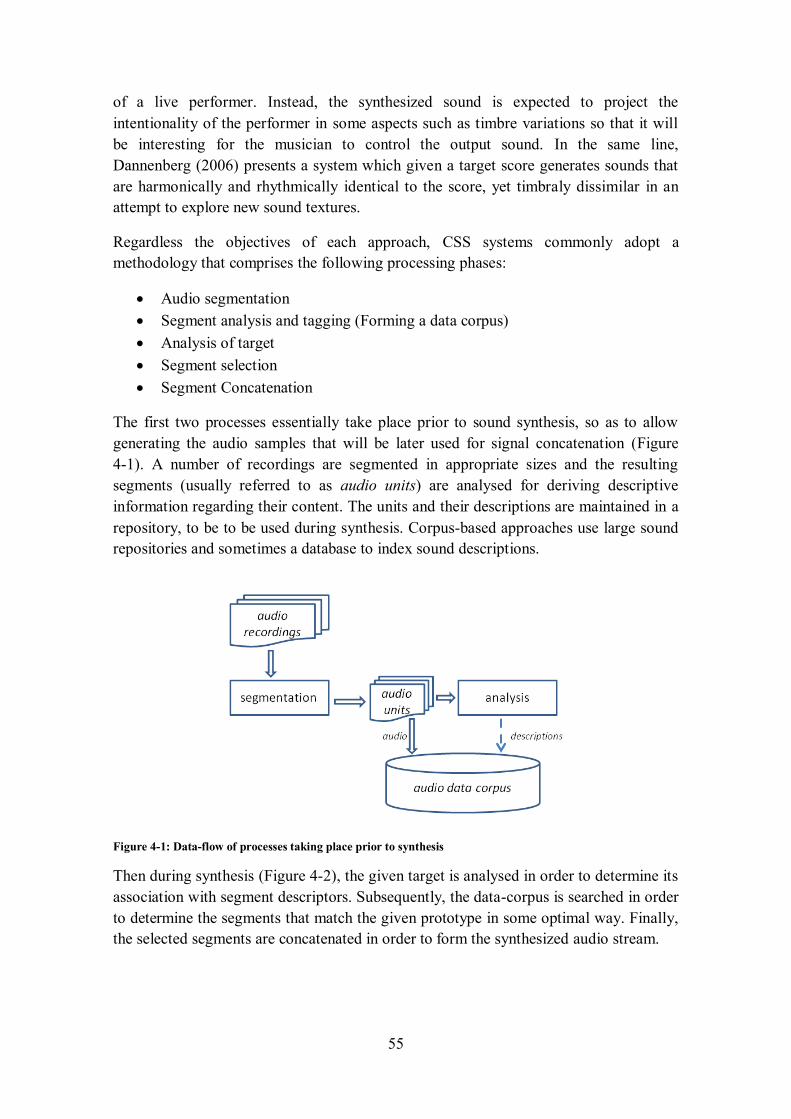
55
of a live performer. Instead, the synthesized sound is expected to project the
intentionality of the performer in some aspects such as timbre variations so that it will
be interesting for the musician to control the output sound. In the same line,
Dannenberg (2006) presents a system which given a target score generates sounds that
are harmonically and rhythmically identical to the score, yet timbraly dissimilar in an
attempt to explore new sound textures.
Regardless the objectives of each approach, CSS systems commonly adopt a
methodology that comprises the following processing phases:
Audio segmentation
Segment analysis and tagging (Forming a data corpus)
Analysis of target
Segment selection
Segment Concatenation
The first two processes essentially take place prior to sound synthesis, so as to allow
generating the audio samples that will be later used for signal concatenation (Figure
4-1). A number of recordings are segmented in appropriate sizes and the resulting
segments (usually referred to as audio units) are analysed for deriving descriptive
information regarding their content. The units and their descriptions are maintained in a
repository, to be to be used during synthesis. Corpus-based approaches use large sound
repositories and sometimes a database to index sound descriptions.
Figure 4-1: Data-flow of processes taking place prior to synthesis
Then during synthesis (Figure 4-2), the given target is analysed in order to determine its
association with segment descriptors. Subsequently, the data-corpus is searched in order
to determine the segments that match the given prototype in some optimal way. Finally,
the selected segments are concatenated in order to form the synthesized audio stream.
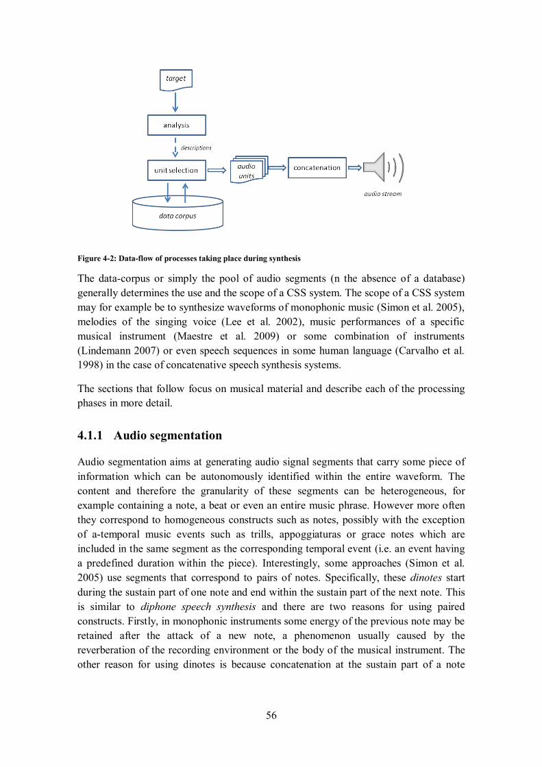
56
Figure 4-2: Data-flow of processes taking place during synthesis
The data-corpus or simply the pool of audio segments (n the absence of a database)
generally determines the use and the scope of a CSS system. The scope of a CSS system
may for example be to synthesize waveforms of monophonic music (Simon et al. 2005),
melodies of the singing voice (Lee et al. 2002), music performances of a specific
musical instrument (Maestre et al. 2009) or some combination of instruments
(Lindemann 2007) or even speech sequences in some human language (Carvalho et al.
1998) in the case of concatenative speech synthesis systems.
The sections that follow focus on musical material and describe each of the processing
phases in more detail.
4.1.1 Audio segmentation
Audio segmentation aims at generating audio signal segments that carry some piece of
information which can be autonomously identified within the entire waveform. The
content and therefore the granularity of these segments can be heterogeneous, for
example containing a note, a beat or even an entire music phrase. However more often
they correspond to homogeneous constructs such as notes, possibly with the exception
of a-temporal music events such as trills, appoggiaturas or grace notes which are
included in the same segment as the corresponding temporal event (i.e. an event having
a predefined duration within the piece). Interestingly, some approaches (Simon et al.
2005) use segments that correspond to pairs of notes. Specifically, these dinotes start
during the sustain part of one note and end within the sustain part of the next note. This
is similar to diphone speech synthesis and there are two reasons for using paired
constructs. Firstly, in monophonic instruments some energy of the previous note may be
retained after the attack of a new note, a phenomenon usually caused by the
reverberation of the recording environment or the body of the musical instrument. The
other reason for using dinotes is because concatenation at the sustain part of a note

57
reduces undesired audible artefacts (e.g. discontinuities perceived as glitches) which are
often unavoidable when concatenating at the location of note onsets (Schwarz 2007).
Different systems use different segmentation methodologies. Some even use manual
segmentation (Lindemann 2007; Simon et al. 2005). However, as manual segmentation
is labour intensive and therefore constrains the scalability of a CSS system to using
additional audio material, the majority of approaches use automatic segmentation
algorithms.
Automatic segmentation algorithms are commonly distinguished in two categories:
blind segmentation and segmentation by alignment. Blind segmentation algorithms do
not take into account any prior information about the signal or the information carried
within the signal. They commonly compute a number of acoustic features for detecting
note onsets or pitch changes (Lazier and Cook 2003). Alternatively, segmentation by
alignment may be performed by score matching (see section 3.2.2), which can be used
to reveal the boundaries of note or a phrase (Schwarz 200b).
4.1.2 Segment analysis and tagging
Each of the audio units produced during segmentation, normally undergoes an analysis
process which allows determining segment characteristics and therefore associating it
with appropriate descriptions within the pool of audio segments or the database. In
certain cases, the number of audio segments is generally small; their selection is pre-
determined and mere indexing takes place instead of analysis and tagging. Such a case
is for example presented when reconstructing a certain piece of music by concatenating
the segments of a pre-existing reference performance, as in the present work.
However in the majority of CSS systems, each audio segment is tagged with
information accounting for multiple levels of description. Schwarz (2007) discerns three
levels of descriptors which are categorical, static and dynamic. Categorical descriptors
concern the category of musical sounds to which an audio unit belongs and are usually
provided as manual annotations. Categorical descriptors may for example be the
instrument class or some subjective metadata such as ‘mellow’, ‘bright’ etc. Static
descriptors are values that are constant over the entire duration of a unit and they
commonly correspond to perceptual attributes such as pitch or duration. Dynamic
descriptors on the other hand are those having a temporal evolution within an audio unit
and they are usually represented as feature vectors. Examples are the fundamental
frequency, the signal energy or some other time or spectral domain feature.
In some cases not just the description of samples is considered, but also the musical
context within which they occur. For instance in the work of Maestre et al. (2009),
where the emphasis is on rendering musical expressivity, each note segment is
associated with information such as the metrical strength in which it appears and the
pitch of the preceding and the successive note.
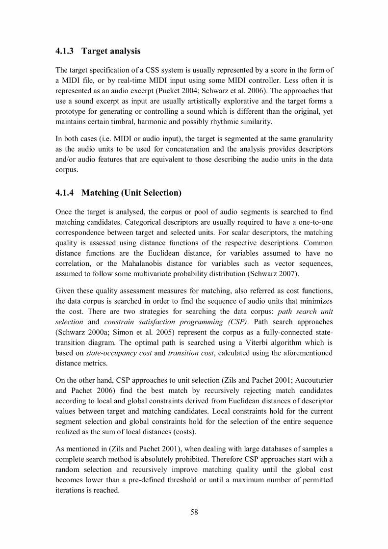
58
4.1.3 Target analysis
The target specification of a CSS system is usually represented by a score in the form of
a MIDI file, or by real-time MIDI input using some MIDI controller. Less often it is
represented as an audio excerpt (Pucket 2004; Schwarz et al. 2006). The approaches that
use a sound excerpt as input are usually artistically explorative and the target forms a
prototype for generating or controlling a sound which is different than the original, yet
maintains certain timbral, harmonic and possibly rhythmic similarity.
In both cases (i.e. MIDI or audio input), the target is segmented at the same granularity
as the audio units to be used for concatenation and the analysis provides descriptors
and/or audio features that are equivalent to those describing the audio units in the data
corpus.
4.1.4 Matching (Unit Selection)
Once the target is analysed, the corpus or pool of audio segments is searched to find
matching candidates. Categorical descriptors are usually required to have a one-to-one
correspondence between target and selected units. For scalar descriptors, the matching
quality is assessed using distance functions of the respective descriptions. Common
distance functions are the Euclidean distance, for variables assumed to have no
correlation, or the Mahalanobis distance for variables such as vector sequences,
assumed to follow some multivariate probability distribution (Schwarz 2007).
Given these quality assessment measures for matching, also referred as cost functions,
the data corpus is searched in order to find the sequence of audio units that minimizes
the cost. There are two strategies for searching the data corpus: path search unit
selection and constrain satisfaction programming (CSP). Path search approaches
(Schwarz 2000a; Simon et al. 2005) represent the corpus as a fully-connected state-
transition diagram. The optimal path is searched using a Viterbi algorithm which is
based on state-occupancy cost and transition cost, calculated using the aforementioned
distance metrics.
On the other hand, CSP approaches to unit selection (Zils and Pachet 2001; Aucouturier
and Pachet 2006) find the best match by recursively rejecting match candidates
according to local and global constraints derived from Euclidean distances of descriptor
values between target and matching candidates. Local constraints hold for the current
segment selection and global constraints hold for the selection of the entire sequence
realized as the sum of local distances (costs).
As mentioned in (Zils and Pachet 2001), when dealing with large databases of samples a
complete search method is absolutely prohibited. Therefore CSP approaches start with a
random selection and recursively improve matching quality until the global cost
becomes lower than a pre-defined threshold or until a maximum number of permitted
iterations is reached.
59
4.1.5 Concatenation
Subsequent to unit selection, unit concatenation takes place in order to generate the
synthesized waveform. Clearly, some blending needs to be applied at the junction point
of consecutive units in order to avoid signal discontinuities resulting in audible clicks.
Such blending may range from a simple amplitude cross-fade (Dannenberg 2006), to
more sophisticated phase and spectral shape interpolation techniques (Bonada and
Loscos 2003).
Furthermore, in some cases (Maestre et al. 2009), unit transformation may take place
prior to concatenation so that the selected units will better match the desired target
concerning amplitude, pitch or duration. Although amplitude scaling is straightforward,
pitch and duration transformations commonly use phase vocoder techniques (Flanagan
and Golden 1966), as in (Bonada and Serra 2007), or some variation of the Pitch
Synchronous Overlap – Add transform (Roucos and Wilgus 1985), as in Simon et al.
(2005).
4.2 Concatenation in speech synthesis and coding
From an engineering perspective, concatenative sound synthesis has its origins in
speech synthesis, where signal concatenation is an established technique for offering
improved naturalness and intelligibility of synthesized voice compared to alternative
parametric models of speech (Sak et al. 2006; Bulut et al. 2002). It is therefore essential
to outline here some relevant approaches from the speech synthesis domain.
Figure 4-3: Classification of text-to-speech synthesis techniques

60
Text-To-Speech (TTS) synthesis is broadly classified in parametric and corpus-based
approaches (Figure 4-3). Parametric approaches generate a speech waveform based on
signal and physical modelling. For example formant synthesis is based on filtering
sinusoidal or noise components in order to better simulate the spectral envelope of vocal
utterances. Accordingly, articulatory synthesis approaches use a physical model to
simulate the flow of air in the vocal tract. In contrast, corpus-based approaches use a
pool of pre-recorded speech segments that approximate the target speech signal. In this
respect, three approaches may be found in the relevant literature (Dutoit 2008): fixed-
inventory, unit selection and statistical parametric (or HMM) synthesis. In fixed
inventory approaches the data corpus consists of small snippets of voice sounds that
correspond to phonemes, diphones or syllables. Unit selection approaches use much
larger databases for which each speech utterance is represented by several segments of
speech corresponding to different segmentation granularities. Therefore the data corpus
contains sounds ranging from diphones and syllables to words or entire sentences.
During waveform generation, a ‘unit selection’ algorithm is employed in order to find
the chain of units that best accounts for the target prototype. This type of synthesis
yields improved naturalness and intelligibility compared to fixed inventory approaches,
as the segments that are finally selected for concatenation capture not only the phonetic
content but also the contextual and prosodic characteristics of the target signal. Finally,
in statistical parametric coding or simply HMM synthesis, the speech corpus is used for
training an HMM that relates speech utterances to parametric representations
corresponding to pitch, intonation and duration information (Zen et al. 2009). During
synthesis, the speech waveform is generated using the induced parametric
representation of sound and some parametric approach such as formant or articulatory
synthesis. Therefore HMM speech synthesis is not a concatenative approach in respect
with waveform generation.
Besides TTS, concatenative sound synthesis may also be utilized for low bit-rate speech
coding. Generally, speech coding concerns the compression of speech signals for the
purposes of transmitting them over low-bandwidth communication channels as in
mobile or Voice over IP communications, and is thereby highly relevant to the present
work. There are several approaches to speech coding and they may be classified
according to a number of attributes (Spanias 1994; Hasegawa and Alwan 2003).
Roughly they can be divided into waveform coders and model based or parametric
coders (or vocoders). Waveform coders are based on removing the statistical
redundancies of the signal and do not assume any prior knowledge about the signal
generation mechanism. Typical examples of waveform coders are based on Pulse Code
Modulation (PCM) such as Differential PCM (DPCM) and Adaptive Differential PCM
(ADPCM) as well as Delta Modulation. They have relatively low complexity in the
encoding process but yield higher bit-rates (16-64 kbps) in comparison to other
encoding schemes (Hasewaga and Alwan 2003). Vocoders on the other hand are
speech-specific perceptual coders, as they aim at rejecting perceptual redundancies in
the speech signals. Vocoders are capable of providing intelligible speech at bitrates 2.4
kbps and below, but cannot provide natural sounding speech at any bit rate. Typical
61
examples are Homophonic Vocoders, Formant Vocoders encompassing spectral
envelop modelling techniques and Linear Predictive Coders (LPC) using analysis,
synthesis and articulatory models to model the speech signal.
In speech coding, a third category is defined by hybrid coders, which exploit the
advantages of both strategies (i.e. waveform and speech-specific coders). Modern
hybrid coders can achieve communication quality speech at 8 kbps and below at the
expense of increased complexity. There are several hybrid codecs including the CELP
(Code-Excited Linear Prediction) codec (Schroeder and Atal 1985), which is one of the
most widely used speech codec.
Yet a further category of speech codecs, mostly relevant to the present work are
segmental speech coders, also known as very-low bitrate (VLBR) speech coders or
corpus-based coders. In segmental voice coding, feature vectors are calculated for
segments of the speech signal to be encoded. These feature vectors are compared to the
pre-calculated feature vectors of speech segments residing in a database. The index of
the segment in the database which is closest to the original segment is transmitted. To
recreate the speech signal, the successive transmitted indices are mapped to speech
segments which are subsequently concatenated to reproduce the original speech
waveform. Approaches to segmental speech coding were presented since the late 90s
(Cernocky, Baudoin and Chollet 1998).
Segmental coders achieve extremely low bit rates but have the disadvantage of being
speaker dependent and have high memory costs due to the size of the speech corpus.
However, Baudoin and El Chami (2003) presented a speech coder which achieves a
bitrate of 400bps using a speech corpus summing in one hour of speech. Another reason
assumed to have hindered the proliferation of segmental codecs is related to the fact that
these codecs generally yield variable bit rates, which is unacceptable in certain
communication applications involving low bandwidth channels with their limit on
maximum rate. However, some recent approaches have presented algorithms for
employing segmental coding at fixed rates (e.g. Kumar et al. 2008). Moreover,
segmental coders are considered rather unsuitable for real-time applications (e.g.
teleconferencing) due to the computational complexity of unit selection algorithms,
even though relevant optimizations have been occasionally proposed (Roucos et al.
1987).
4.3 Contemporary Relevant Initiatives
In the music domain, concatenative synthesis has attracted a lot of research interest for
more than a decade. Comprehensive reviews on the origins and the evolution of relevant
research initiatives have been published in dedicated scholar publications (Schwarz
2006; Schwarz 2007). Hence, there is no need to reproduce another such review in this
section. Instead, the present section will focus on understanding the current state of the
62
art, so as to gain insight on the best practices that may be applicable to our target
domain of Networked Music Performance.
Like most directions in computer music research, the focus of concatenative music
synthesis is either to compositionally explore new sound textures or to efficiently
reproduce musical acoustics. Clearly, the target application of the present work belongs
to the second category of approaches, thus emphasising on reproducing musical
expression as faithfully as possible. Furthermore, the present work has to deal with two
further challenges: firstly the target prototype to be synthesized is provided as an audio
signal (instead of a symbolic representation) and secondly both analysis of target as well
as re-synthesis must take place within strict time constraints imposed by the EPT of
30ms (see section 2.4), therefore qualifying the system under investigation as a real-
time system.
No research initiatives attempting to satisfy all three requirements (i.e. faithful
instrumental synthesis, audio target and real-time operation) have been reported in the
relevant literature thus far. It will be seen that audio target and real-time operation has
been attempted exclusively in compositionally explorative approaches, therefore not
having the requirement of high fidelity audio renditions.
Both compositional and high-fidelity approaches are presented below, in attempt to gain
understanding on the challenges of the present work. The following two subsections
outline some of the most relevant approaches for both approaches. Then, the section that
follows provides a comparison of the presented systems in order to emphasize on their
similarities and differences.
4.3.1 Compositional approaches
This section reports on three research initiatives that focus on explorative music
composition by means of sample concatenation. Specifically, the aim is not to
accurately reproduce acoustic sounds but instead to produce interesting textures that
retain some perceptual relevance to the given audio or symbolic target.
These initiatives are considered relevant to this dissertation only because they allow for
synthesizing an output while the input is acquired, and are therefore presented as real-
time CSS approaches.
4.3.1.1 Jamming with Plunderphonics
Aucouturier and Pachet (2006) present a real-time interactive extension of their older
work on Musical Mosaicing (Zils and Pachet 2001). The output sound is generated in
real-time from MIDI or audio input using a Constraint Satisfaction Programming
technique (section 4.1.4) and constraints that may be asynchronously added or removed
to a CPS solver module. The article presents an example application in which a virtual
drummer is able to interact with real-time MIDI input. This is not a case of musical
accompaniment, it rather uses MIDI input (e.g. from keyboard) to control the drum
63
beats that are selected for audio playback, according to the energy and pitch values of
the MIDI controller, based on the previously provided constraints.
The sound units correspond to 4 –beat drum samples automatically segmented from
drum solos of popular or jazz music pieces. The drum solos within the piece are also
automatically detected. They do not report on any specific transformation such as phase
vocoder taking place prior to synthesis, presumably due to the percussive nature and
noisy content of drum sounds.
This work is classified in compositional approaches as it does not aim at simulating a
specific instrumental sound. It is rather meant as an explorative, controlled synthesis
system.
4.3.1.2 CataRT
CataRT (Schwarz et al. 2006) is a real-time extension of the Caterpillar system, which
was developed by Schwarz (2004) for his PhD dissertation. CataRT plays grains from a
large corpus of segmented and descriptor-analysed sounds according to their proximity
to a target position in the descriptor space. The target application is described as an
‘interactive explorative synthesis’ approach. It allows exploring the corpus interactively
or via a target audio file, a live audio input or through gestural control. CataRT is
implemented in MaxMSP and is distributed as free and open source software under a
GNU GPL10
licence.
Audio units are segmented from violin sounds, environmental noises and speech.
Segmentation is achieved by audio-to-score alignment in the case of musical sounds,
and by blind segmentation for the other sounds. Units are annotated using the MPEG-7
low level descriptor set and indexed in a relational SQL database. Unit selection is
achieved using a Viterbi path-search algorithm that seeks to minimize the Euclidean
distance between the descriptors of the target and those of the database units. A short
fade-in and fade out is applied to the selected units. It is also reported that pitch and
loudness transformations are possible prior to unit concatenation.
4.3.1.3 Input-Driven explorative synthesis
This section refers to the work of Puckette (2004). This work is considered relevant to
the present context because synthesis is driven by real-time audio input. The reported
application scenario concerns the possibility of producing sounds that have similar
timbral variations as the input sound. The sound units were based on vocal recordings
that were analyzed in 30ms time frames to yield 11 frequency bands. The output of
these bands was subsequently used to form a 10-dimensional timbre space, by means of
multidimensional scaling. During synthesis the trajectory of the input sound on the same
timbre space was used to derive the sound units by minimizing the Euclidean distance
between the analyzed and the re-synthesized timbre. Finally, the output sound was
formed by concatenating the selected units using phase vocoder overlap-add. The shape
10 GNU General Public License - http://www.gnu.org/licenses/gpl.html
64
of the controlling input sound could be identified in the output, while the output did not
maintain any phonetic intelligibility.
4.3.2 High fidelity instrumental simulation
This section focuses on the currently most popular CSS solutions that aim at efficiently
rendering the performance of acoustic instruments. These systems are clearly more
relevant to the system under investigation. However in most cases synthesis takes place
offline. The only exception is the Synful synthesizer, for which the target specification
may be provided from a MIDI keyboard in real-time. In this real-time approach, no
audio analysis needs to take place prior to unit selection and concatenation.
4.3.2.1 Expressive Performance of monophonic Jazz Recordings
The system described by Maestre et al. (2009) aims at rendering expressive saxophone
recordings given a music score. It uses a database of automatically segmented
recordings at note level. Notes are blindly segmented using onset features and
fundamental frequency estimation. The resulting segments are annotated using different
levels of description. Apart from conventional melodic descriptors (i.e. pitch, duration,
loudness and some spectral features indicating timbre variations), the system
additionally uses descriptors concerning intra-note structure and transition duration.
This information is acquired by automatic intra-note segmentation using envelop
characterization. Moreover, an additional type of descriptors, of particular importance to
expressive performance rendering, is the context within which an audio segment occurs.
Contextual descriptors are, for instance, the metrical strength in which the segment
appears and the pitch and duration of the previous and the following notes. All these
descriptors are finally processed by a k-means clustering algorithm which clusters note
segments in groups that are likely to be perceptually similar. The cluster label is stored
as an additional descriptor of the note segment.
Rendering musical expression in this work is informed by Narmour’s (1990)
implication/realization theory. Contextual descriptors are informed by three Narmour
structures declaring the expectations created by a note segment. Narmour’s structures
are based on melodic expectations created by intervallic difference and registral
direction (upward or downward interval) between consecutive notes.
Subsequently to audio database construction, the solo recordings that were used to
produce the segments together with the cluster labels of the notes are used to train
expressive performance models using inductive logic programming. During synthesis,
the given score is enriched by predictions of the expressive performance models,
yielding not only pitch and loudness contained in the score but further parameters
regarding expression such as note energy and articulation.
Following, for each note in the score a candidate list of all possible matching segments
is generated. Then, the best matching segment is determined by applying a path-search
algorithm considering both the “cost” of the transformations to be applied and also the
65
concatenation cost. Each retrieved note is transformed in terms of amplitude, pitch and
duration in order to better match the required expressivity. Finally, the transformed
units are concatenated using amplitude and spectral-shape interpolation so as to
eliminate undesirable signal discontinuities.
4.3.2.2 Synful Orchestra
Synful Orchestra11
is a commercial software application providing expressive musical
performances in response to MIDI file (‘look-ahead mode’) or real-time input generated
by a controller such as a keyboard (‘live-mode’). It is used by composers and
performers as a ‘virtual orchestra in a box’. The emphasis is placed on faithfully re-
synthesizing the idiomatic use of music articulation found in note transition-slurs, legato
playing, bow changes etc.
The audio corpus consists of pre-recorded audio passages instead of isolated notes.
These passages are acquired from solo recordings that represent all kinds of articulation
and phrasing: detached, slurred, portamento, sharp attacks, soft attacks, etc. The
recorded phrases are manually annotated, using a graphical editing tool. Their
descriptive labels concern pitches, length and intensity of notes as well as type of note
transitions. During synthesis, the input MIDI stream is parsed to identify musical
phrases consisting of two to eight notes. Subsequently, the corpus is searched for a
matching phrase using a path search algorithm. The selection of matches is based on the
description of pitch, duration and transition type of the phrases contained in the corpus.
As it is highly unlikely that an exact match will be found in the database,
transformations such as intensity, pitch and duration stretching and shifting, take place
prior to synthesis. During synthesis, pitches, amplitudes and durations identified from
the MIDI input stream are generated using additive synthesis. On this additive, ‘tonal’
signal the phrases that were selected from the database are superimposed to give the
final realistic result. This technique is referred as Reconstructive Phrase Modelling
(RPM) by its inventor (Lindemann 2007).
In ‘live-mode’, the system has no advance knowledge of when a new note is coming,
and so it does its best to react as expressively as possible with low latency when a new
note occurs, using only past history of the input stream as a guide to phrasing.
4.3.2.3 Vocaloid
Bonada and Serra (2007) in cooperation with Yamaha, have been working on a software
synthesizer, the Vocaloid12
. The objective of this research is to synthesize expressive
performances of the singing voice given the song lyrics and the music score.
The system, based on phase-vocoder techniques and spectral concatenation, searches the
most convenient sequence of diphonemes (samples) of an annotated database of singing
voice excerpts, recorded at different tempi and dynamics, to render the performance.
These segments are produced from singer recordings which are further segmented by
11 http://www.synful.com/ 12 http://www.vocaloid.com/en/
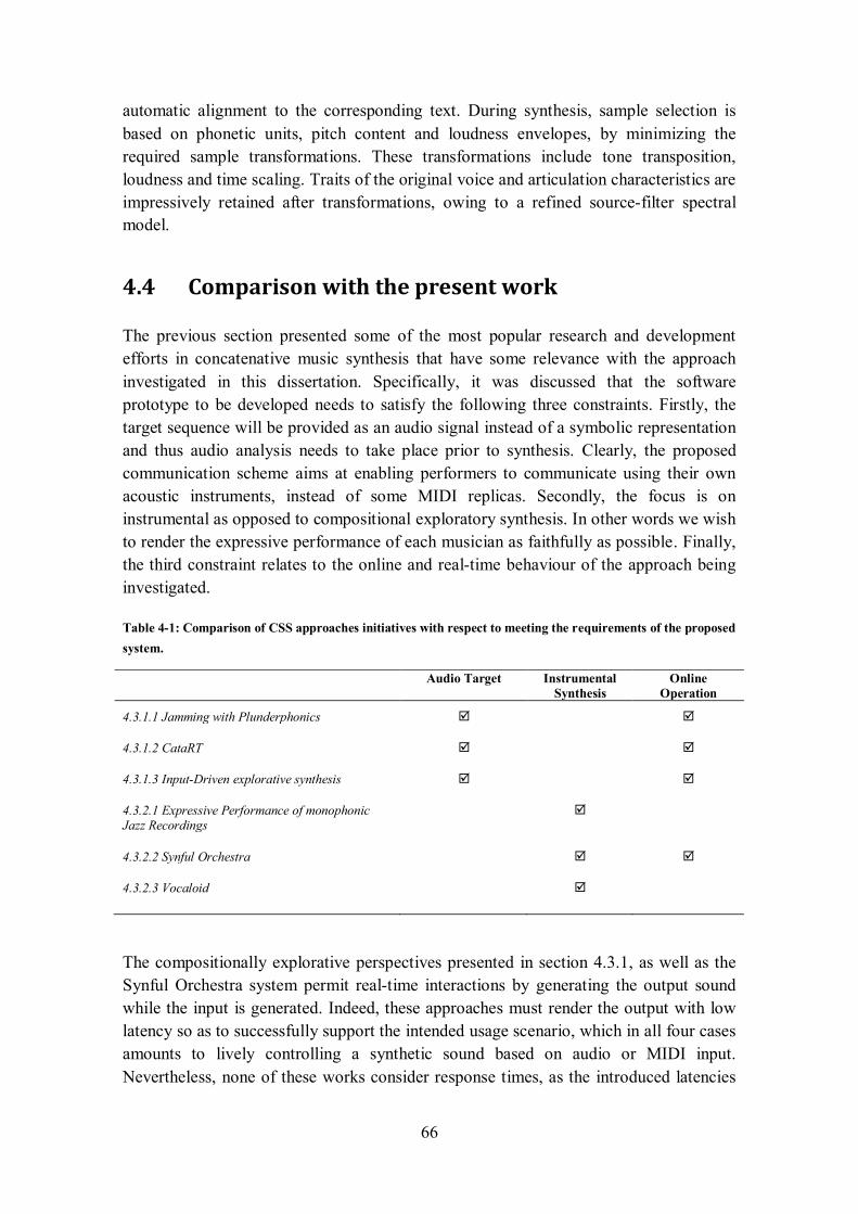
66
automatic alignment to the corresponding text. During synthesis, sample selection is
based on phonetic units, pitch content and loudness envelopes, by minimizing the
required sample transformations. These transformations include tone transposition,
loudness and time scaling. Traits of the original voice and articulation characteristics are
impressively retained after transformations, owing to a refined source-filter spectral
model.
4.4 Comparison with the present work
The previous section presented some of the most popular research and development
efforts in concatenative music synthesis that have some relevance with the approach
investigated in this dissertation. Specifically, it was discussed that the software
prototype to be developed needs to satisfy the following three constraints. Firstly, the
target sequence will be provided as an audio signal instead of a symbolic representation
and thus audio analysis needs to take place prior to synthesis. Clearly, the proposed
communication scheme aims at enabling performers to communicate using their own
acoustic instruments, instead of some MIDI replicas. Secondly, the focus is on
instrumental as opposed to compositional exploratory synthesis. In other words we wish
to render the expressive performance of each musician as faithfully as possible. Finally,
the third constraint relates to the online and real-time behaviour of the approach being
investigated.
Table 4-1: Comparison of CSS approaches initiatives with respect to meeting the requirements of the proposed
system.
Audio Target Instrumental
Synthesis
Online
Operation
4.3.1.1 Jamming with Plunderphonics
4.3.1.2 CataRT
4.3.1.3 Input-Driven explorative synthesis
4.3.2.1 Expressive Performance of monophonic Jazz Recordings
4.3.2.2 Synful Orchestra
4.3.2.3 Vocaloid
The compositionally explorative perspectives presented in section 4.3.1, as well as the
Synful Orchestra system permit real-time interactions by generating the output sound
while the input is generated. Indeed, these approaches must render the output with low
latency so as to successfully support the intended usage scenario, which in all four cases
amounts to lively controlling a synthetic sound based on audio or MIDI input.
Nevertheless, none of these works consider response times, as the introduced latencies
67
do not really render the intended application unusable. Therefore these systems cannot
be literally considered as real-time approaches.
Table 4-1 summarises the features of the presented systems with respect to satisfying
the three constraints of the system under investigation. It can be seen that none of the
currently popular approaches in concatenative synthesis satisfies all three constraints.
Yet, these systems present a number of alternative novelties that can inform current and
future implementations of the proposed system.
All of the approaches aiming at exploratory composition place the research focus on
unit selection algorithms. As unit selection determines the type of perceptual similarities
to be retained in the output sound, it is made clear that the synthesized sound must be
compositionally interesting instead of presenting a faithful rendition of the input. On the
other hand, in high-level instrument synthesis approaches the research focus is placed
on the rendering quality of the audio stream and specifically on reproducing the
expressive nuances generated by performers’ gestures and musical instrument
manipulations.
As will be seen in the next part of the dissertation, the system investigated in the present
work does not facilitate an audio corpus of considerable size, neither a database to store
audio units and associated descriptors. The units used for concatenation are acquired
from a prior solo recording of the performer playing the specific piece of music. These
units are automatically segmented and their selection is predetermined. However, as a
future enhancement, and in order to allow for arbitrary interactions among distributed
musicians a data corpus of previous recordings for each performer will need to be
generated. Consequently, real-time unit selection algorithms must be employed so as to
allow selecting appropriate data units representing the live music stream.
Moreover, the fact that networked musical interactions take place in real-time, presents
a limitation on the quality of concatenation. Specifically, in high-level instrument
synthesis approaches (section 4.3.2), transformation of units always takes place prior to
concatenation so as to alleviate cope with two problems: differences in amplitude, pitch
or duration between the selected unit and the desired output, and perceivable
discontinuities between successive sound units. Within the real-time requirements of the
present system it is impossible to perform sophisticated transformations, unless a
prediction mechanism is incorporated. Consequently, the point of concatenation needs
to be predicted before it actually occurs on the input sound. This issue and the approach
adopted by the system under investigation are discussed explicit in Chapter 9.
68
PART II:
RESEARCH METHODOLOGY
69
5 Research Focus and System Overview
This chapter elucidates the research focus of the present dissertation and provides an
overview of the adopted methodology and the prototype software application to be
developed. The first section recapitulates on the conclusions of the previous chapters
and illustrates the objectives of the present work. Following, the computational
challenges of achieving these objectives are enumerated. The final section presents the
overall methodology and the block diagram of the prototype system to be developed.
5.1 Rationale and Objective
The effectiveness of NMP systems to offer musical collaborations comparable to those
of collocated music performances is constrained by two types of problems (section 2.2).
The first relates to the availability of network resources, while the second concerns the
lack of suitable software tools and interfaces for permitting distributed musicians to
effectively collaborate across distance (section 2.6).
On the other hand, machine listening approaches aim at offering computational
affordances that can significantly assist or enhance the experience of musicians during
live performance. For example, automatic music transcription, audio alignment and
computer accompaniment present innovative system capabilities both in offline as well
as in online settings. As real-time functionalities, they can augment the experience of
musicians in several music performance contexts, such as learning, jamming,
rehearsing, etc. The perspective of encompassing capabilities of machine musicianship
systems in the context of NMP research has not been widely addressed (section 3.3).
In a similar line, a number of initiatives in concatenative music synthesis research aim
at rendering expressive music performances. Unfortunately, the relevant initiatives are
rarely implemented in real-time settings, and even if they are, a symbolic description of
the sound to be synthesized is provided instead of an audio stream (section 4.4).
The objective of the present work is to explicitly suggest the exploitation of
contemporary research achievements in the areas of machine listening and
concatenative music synthesis, so as to alleviate from the complexities of NMP systems.
In fact, it could be that progress made in one domain can directly translate to the other
domains. So for example, making progress on expressive performance rendering by
means of audio segment concatenation, can directly translate to improving computer
accompaniment. Improving computational models of musical expectation and
anticipation directly suggests the possibility of eliminating communication latencies,
which is the main barrier of communication in NMP systems. Progress in NMP allows
investigating features of man-machine collaboration also applicable to machine
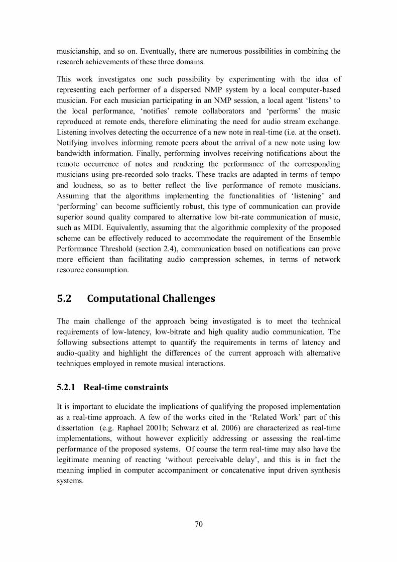
70
musicianship, and so on. Eventually, there are numerous possibilities in combining the
research achievements of these three domains.
This work investigates one such possibility by experimenting with the idea of
representing each performer of a dispersed NMP system by a local computer-based
musician. For each musician participating in an NMP session, a local agent ‘listens’ to
the local performance, ‘notifies’ remote collaborators and ‘performs’ the music
reproduced at remote ends, therefore eliminating the need for audio stream exchange.
Listening involves detecting the occurrence of a new note in real-time (i.e. at the onset).
Notifying involves informing remote peers about the arrival of a new note using low
bandwidth information. Finally, performing involves receiving notifications about the
remote occurrence of notes and rendering the performance of the corresponding
musicians using pre-recorded solo tracks. These tracks are adapted in terms of tempo
and loudness, so as to better reflect the live performance of remote musicians.
Assuming that the algorithms implementing the functionalities of ‘listening’ and
‘performing’ can become sufficiently robust, this type of communication can provide
superior sound quality compared to alternative low bit-rate communication of music,
such as MIDI. Equivalently, assuming that the algorithmic complexity of the proposed
scheme can be effectively reduced to accommodate the requirement of the Ensemble
Performance Threshold (section 2.4), communication based on notifications can prove
more efficient than facilitating audio compression schemes, in terms of network
resource consumption.
5.2 Computational Challenges
The main challenge of the approach being investigated is to meet the technical
requirements of low-latency, low-bitrate and high quality audio communication. The
following subsections attempt to quantify the requirements in terms of latency and
audio-quality and highlight the differences of the current approach with alternative
techniques employed in remote musical interactions.
5.2.1 Real-time constraints
It is important to elucidate the implications of qualifying the proposed implementation
as a real-time approach. A few of the works cited in the ‘Related Work’ part of this
dissertation (e.g. Raphael 2001b; Schwarz et al. 2006) are characterized as real-time
implementations, without however explicitly addressing or assessing the real-time
performance of the proposed systems. Of course the term real-time may also have the
legitimate meaning of reacting ‘without perceivable delay’, and this is in fact the
meaning implied in computer accompaniment or concatenative input driven synthesis
systems.

71
However, more formally and in the context of digital signal processing, a real-time
system has to at least satisfy the following two requirements (Kuo, Lee and Tian 2006):
a) The system must be causal. Causality implies that at any time only the current
and the previous values of the system are available. The term online, used
throughout this document refers to causal behaviour.
b) The required processing latency per each input frame should be less than or
equal to the time span represented by that frame for all possible frame lengths.
In other words the average processing time per sample should be no longer than
the sampling period.
Clearly, the first of these requirements has an influence on the robustness of the
implemented algorithms. This is primarily caused by the fact that no signal overview is
available prior to processing and therefore operations such as DC removal or signal
normalization are not possible. Moreover, as most of the algorithms considered here are
essentially statistical, data distribution measures such as means and variances are
computed from insufficient data and are therefore suboptimal to those computed from
offline procedures.
The second constraint demands using algorithms of reduced computational complexity
such that processing latencies do not exceed the time corresponding to the length of the
audio buffer. For instance, processing a block of 1024 samples of monophonic 16-bit
audio with a rate of 44.1 kHz should not require more time than 23.22ms to execute on
the target processing machine, otherwise processing becomes ineffective as audio
blocks are collected faster than processed, thus necessitating to queue them in an ever
increasing memory stack.
In addition to the above constraints, the target application scenario presents a third
limitation. Specifically, in NMP settings the sum of the latencies of all the processes in
the capture-analysis-transmission-reception-synthesis-playback cycle must be kept
below the Ensemble Performance Threshold (EPT), i.e. approximately below 30ms (see
also section 2.4), including buffering delays. This third constraint enforces limitations
not only in processing latencies but also on the length of the audio buffers. For example,
buffering in blocks of 1024 samples at the rate of 44.1 kHz yields a latency of 23.22ms
which is already close to the EPT and therefore strictly prohibited for the target
application. Consequently, the audio processing algorithms investigated and presented
in this dissertation are constraint to use a maximum block size of 512 samples, which
corresponds to a buffering latency of 11.6ms.
Unfortunately, the limitation imposed on the length of the audio buffer further degrades
the performance of real-time analysis/synthesis algorithms, especially when these
operate on the frequency domain of the signal. Specifically, when applying Fourier
Transforms a 512-samples frame length at the rate of 44.1 kHz results in a linear
frequency resolution of 86.13Hz per frequency band. Consequently at the frequency of
220Hz (i.e. A note before middle C) which lies within the frequency range of most

72
acoustic instruments, the frequency band spans more than four semitones, and therefore
spectral features provide little information about the pitch of the notes being performed.
A common approach to dealing with this problem is to either employ multi-resolution
frequency analysis, as in the wavelet transform (see section 6.6.1), or to attempt
estimating pitch content based on the energy of harmonic overtone structure (section
6.6.2).
When the system is expected to react within certain time limits, as in computer
accompaniment systems, a common practice to reducing latency is to employ prediction
mechanisms. For instance Raphael (2001b) uses Bayesian Belief Networks in order to
predict the performance of a soloist, so as to timely adjust the tempo of the orchestral
accompaniment. This is achieved during an offline training phase, which yields a
performer-specific model for a specific piece of music using past rehearsal recordings.
In a similar line the work of Sarkar and Vercoe (2007), uses a Dynamic Bayesian
Network to predict the next note of a musical phrase on the Indian drum tabla, based on
rules that define rhythmic phrases for the specific instrument and music genre.
As will be seen in Chapter 9, in the present work an alternative mechanism to
progressively predict the energy and duration of a note is employed at the time instant
when its onset occurs. The problem is simplified by assuming that duration and energy
deviations from one performance to another will be consistently propagated based on
the deviations observed on the past four or five notes.
5.2.2 Audio quality constraints
The second challenge to be met by the target system is to maintain high quality audio
communication, comparable to that of live audio stream exchange, while reducing
information bandwidth to significantly low bitrates. Conventionally, low bitrate
communication requires the use of signal descriptions instead of raw audio streams.
When considering acoustic music, descriptive representations are commonly manifested
by the score of a music piece or equivalently its MIDI counterpart. Although highly
compact, such descriptions fail to maintain the expressive aspects of music performed
using acoustic musical instruments.
The focus is clearly on musical acoustics as opposed to performances using electronic
instruments, for which musical communication protocols such as MIDI or the
OpenSound Control provide established solutions in low-bandwidth musical
interactions. As was discussed in the Introduction (section 1.2), the expressive nuances
of music interpretation using acoustic instruments are predominantly attributed to the
idiomatic use of articulation, dynamics and also deviations from predefined musical
tempi (Widmer and Goebl 2004). Such expressive utterances are impossible to
sufficiently reconstruct from any symbolic representation alone. Moreover, the
originality of sound produced by acoustic instrument manipulations is not easy to
replicate when using functional sound synthesis methodologies. Therefore

73
concatenative music synthesis is the single choice in order to preserve the expressive
qualities of musical performance.
In the present context, high-fidelity music synthesis amounts to being able to re-
synthesize the live performance as closely as possible. As the methodology uses a prior
recording of the same piece of music performed by the same performer, retaining the
expressive qualities of the live performance requires careful transformations of the
audio segments to be concatenated in terms of loudness (i.e. dynamics) and duration
(revealing tempo deviations). As for timbral nuances we assume that they are
sufficiently captured in the original solo recording. Clearly, transformations degrade
signal quality and therefore they should be kept as minimal as possible. Furthermore,
careful processing must take place in order to eliminate perceivable artefacts caused by
signal discontinuities at the junction point of consecutive audio segments.
Equivalently, in the context of NMP undesirable artefacts are caused by audio dropouts
owing to network packet loss (see section 2.5.2.1.3). As in the proposed system
bandwidth requirements are fairly eliminated, packet loss can be entirely eliminated by
transmitting redundant information in addition to onset notifications. Clearly, it is not
acceptable to eliminate distortions that are commonly found in NMP and introduce new
types of distortions attributed to segment transformation or signal concatenation.
Consequently, implementing the required transformations and applying them within the
aforementioned time constraints presents a significant challenge for the system under
investigation.
5.3 Assumptions - Prerequisites
Due to the fact that the prototype system developed in the present work has not been
previously investigated in its entity, and in order to efficiently cope with the
aforementioned computational challenges, a number of assumptions are made on the
application context so as to allow for producing some useful research results.
Undoubtedly, these assumptions correspond to usage constraints in their own behalf.
However, eliminating these constraints and providing more generic solutions to the
proposed approach is the main focus of ongoing and future research efforts.
Up to the time of this writing, the proposed approach has been applied to solo
recordings (i.e. assuming a single musician is located at each network node) of
monophonic instruments, although provisions are made for additionally accommodating
polyphonic instruments. Moreover, no unit selection process is involved, other than
concatenating an automatically pre-segmented performance of the reference music
piece.
The entire concept might seem rather simplistic, as the segmentation of the solo
performance to units; the online analysis of the live solo as well as the real-time
concatenation of segments could be performed using a single algorithm for robust real-
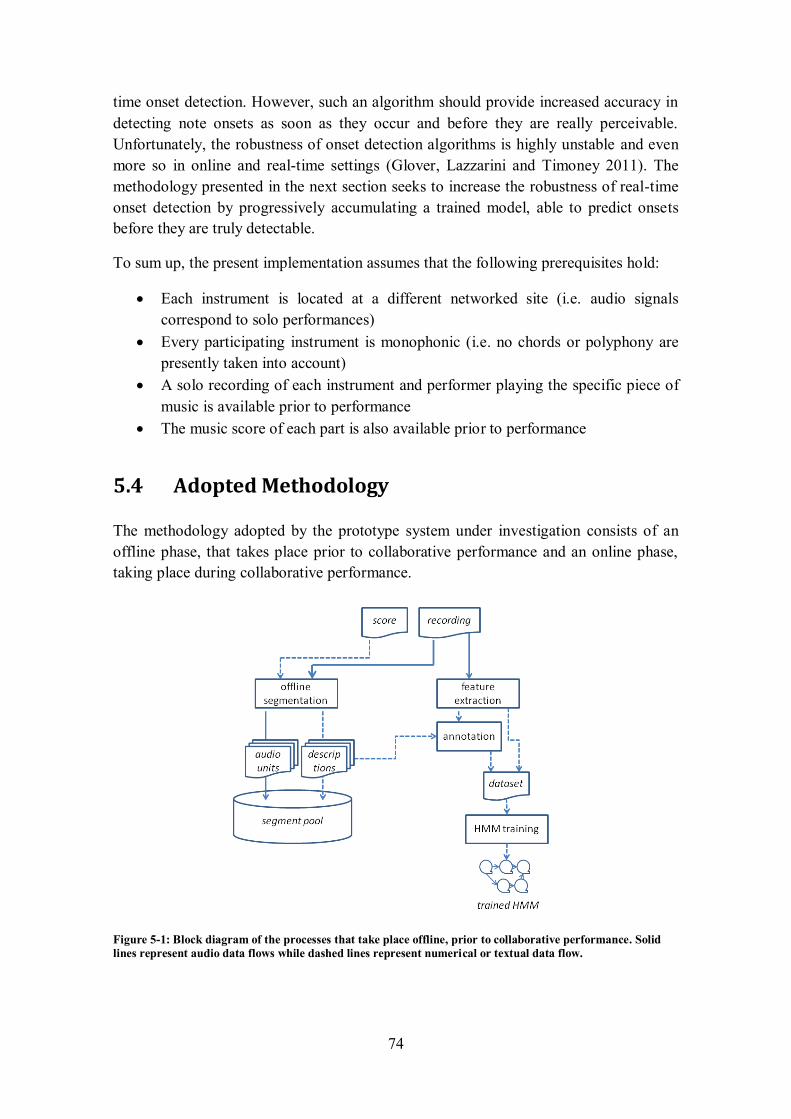
74
time onset detection. However, such an algorithm should provide increased accuracy in
detecting note onsets as soon as they occur and before they are really perceivable.
Unfortunately, the robustness of onset detection algorithms is highly unstable and even
more so in online and real-time settings (Glover, Lazzarini and Timoney 2011). The
methodology presented in the next section seeks to increase the robustness of real-time
onset detection by progressively accumulating a trained model, able to predict onsets
before they are truly detectable.
To sum up, the present implementation assumes that the following prerequisites hold:
Each instrument is located at a different networked site (i.e. audio signals
correspond to solo performances)
Every participating instrument is monophonic (i.e. no chords or polyphony are
presently taken into account)
A solo recording of each instrument and performer playing the specific piece of
music is available prior to performance
The music score of each part is also available prior to performance
5.4 Adopted Methodology
The methodology adopted by the prototype system under investigation consists of an
offline phase, that takes place prior to collaborative performance and an online phase,
taking place during collaborative performance.
Figure 5-1: Block diagram of the processes that take place offline, prior to collaborative performance. Solid
lines represent audio data flows while dashed lines represent numerical or textual data flow.
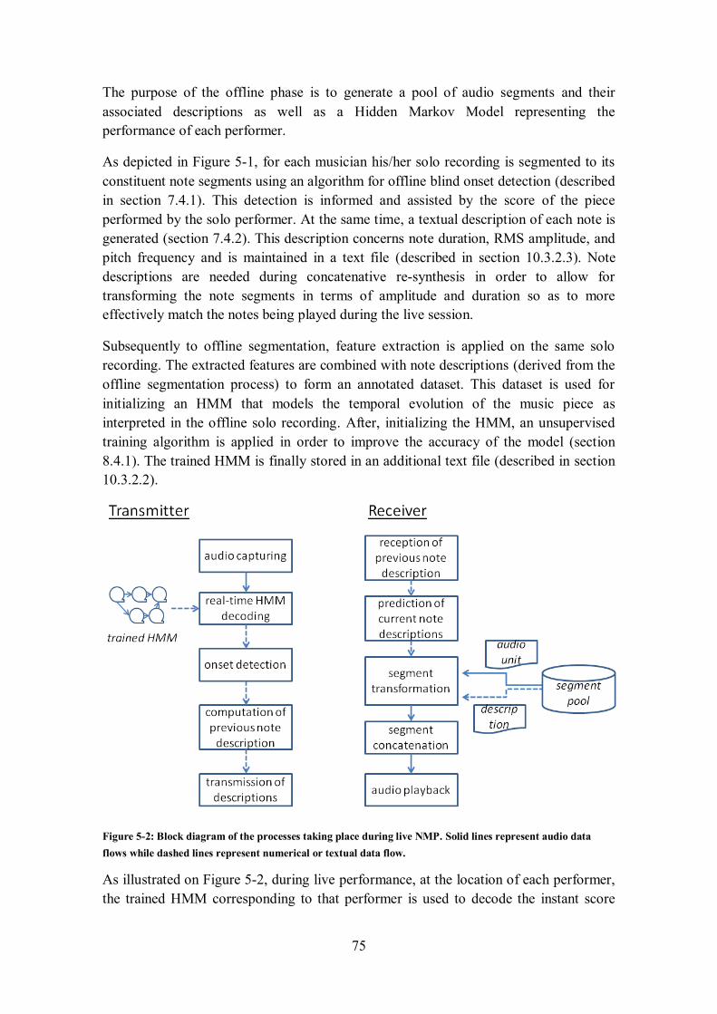
75
The purpose of the offline phase is to generate a pool of audio segments and their
associated descriptions as well as a Hidden Markov Model representing the
performance of each performer.
As depicted in Figure 5-1, for each musician his/her solo recording is segmented to its
constituent note segments using an algorithm for offline blind onset detection (described
in section 7.4.1). This detection is informed and assisted by the score of the piece
performed by the solo performer. At the same time, a textual description of each note is
generated (section 7.4.2). This description concerns note duration, RMS amplitude, and
pitch frequency and is maintained in a text file (described in section 10.3.2.3). Note
descriptions are needed during concatenative re-synthesis in order to allow for
transforming the note segments in terms of amplitude and duration so as to more
effectively match the notes being played during the live session.
Subsequently to offline segmentation, feature extraction is applied on the same solo
recording. The extracted features are combined with note descriptions (derived from the
offline segmentation process) to form an annotated dataset. This dataset is used for
initializing an HMM that models the temporal evolution of the music piece as
interpreted in the offline solo recording. After, initializing the HMM, an unsupervised
training algorithm is applied in order to improve the accuracy of the model (section
8.4.1). The trained HMM is finally stored in an additional text file (described in section
10.3.2.2).
Figure 5-2: Block diagram of the processes taking place during live NMP. Solid lines represent audio data
flows while dashed lines represent numerical or textual data flow.
As illustrated on Figure 5-2, during live performance, at the location of each performer,
the trained HMM corresponding to that performer is used to decode the instant score
76
position of the live performance in real-time (the real-time decoding process is
described in section 8.4.2). If the decoded position corresponds to a note onset, then a
description (the note duration and the RMS amplitude) of the previous note is
communicated to the remaining performers participating in the live session. These
remote peers, upon receiving the description of the previous note, attempt to predict the
attributes (i.e. RMS and duration) of the current note (see section 9.3.1). These
attributes correspond to expressive deviations in tempo and loudness during live
performance. Following, the corresponding note segment is retrieved from the pool of
audio segments along with its description. This segment is transformed so that it better
matches the predictions for the current note (section 9.3.2). Finally, the transformed
segment is concatenated to the audio stream being reproduced (section 9.3.3).
At the location of each participating peer, a single transmitter decoding the local
performance is executed and as many receivers as the other the number of remote peers.
For instance for a session of four performers, at the location of each performer a single
transmitter and another three receivers are instantiated. Low latency audio capturing and
playback is achieved using audio buffers of 512 samples per channel at the sampling
rate of 44.1 kHz, corresponding to a buffering latency of 11.6ms. This latency is a good
compromise between small buffering delays and improved performance of the audio
analysis algorithms.
The following chapters provide details on the precise methodology followed by each of
these processes. Specifically, Chapter 7 describes the offline segmentation process.
Chapter 8 describes the score following process using HMMs, i.e. the ‘listening’
component. The representation of the performance model, the offline training as well as
the process of real-time decoding are presented in detail. Finally, chapter 9 describes the
synthesis process including the type of information transmitted as network notifications
(i.e. the ‘notify’ component), acquisition of predictions for the current note attributes, of
segment transformations to account for tempo and loudness deviations as well as the
technique used for eliminating signal discontinuities at the junction point of consecutive
segments (i.e. the ‘perform’ component). As audio feature extraction is a pre-processing
step employed whenever descriptive information needs to be inferred from an audio
signal, the next chapter 6 describes the feature extraction process and provides the
definitions of the acoustic features that were used for experimentation and
implementation throughout the development of the final system.
77
6 Online Audio Feature Extraction
The present chapter is intended as a reference for the chapters that follow. Specifically,
it provides definitions for a number of audio features that were used throughout this
work, those used during experimentation as well as those that were selected to inform
computations in the final prototype system. Definitions are provided as mathematical
formulas. Besides the mathematical definition, the following sections provide
visualizations of the temporal evolution of each feature for an example melodic phrase.
These visualisations effectively depict the performance of the different features for the
tasks of audio segmentation and audio to score alignment, which are presented in
subsequent chapters.
6.1 Feature extraction and visualisation
In contrast to directly using audio samples, machine listening approaches use a set of
attributes for signal representation, known as audio features. In principle, an audio
feature is a signal property computed over successive audio blocks having a constant
predefined length of the order of 10-50ms. At the sampling rate of 44.1kHz, commonly
used values for the length of audio blocks are those of 2048, 1024 or 512 samples. The
use of blocks having a length of some power of two is imposed by the fact that these
features are often computed on the frequency domain of the signal, which is usually
obtained by the Fourier Transform. The fast implementation of the Fourier transform
(FFT) is based on computational optimisations assuming that the length of the audio
blocks is some power of two.
At this point it is important to disambiguate the use of the terms audio block versus
audio frame. The term frame is sometime used to refer to a small signal chunk.
However, in audio engineering technology the term audio frame is usually used to refer
to a time instance across all audio channels, i.e. 8 channels would result in an audio
frame of 8 samples, one at each audio channel. Hence, when a signal has a single
channel, a frame refers to an audio sample. Throughout the present document the term
audio block will be consistently used, so as to avoid confusion with multichannel audio
frames.
The reason for using audio features, as opposed to signal samples is twofold: firstly
features offer a rate reduction on the data to be processed, and secondly they can be
cautiously selected to effectively reveal the desired structure of the signal depending on
the information that needs to be found. Small block lengths result in increased time
resolution therefore allowing the detection of sudden bursts of feature values even if
they span short time intervals. Unfortunately, as already elaborated (section 5.2.1),
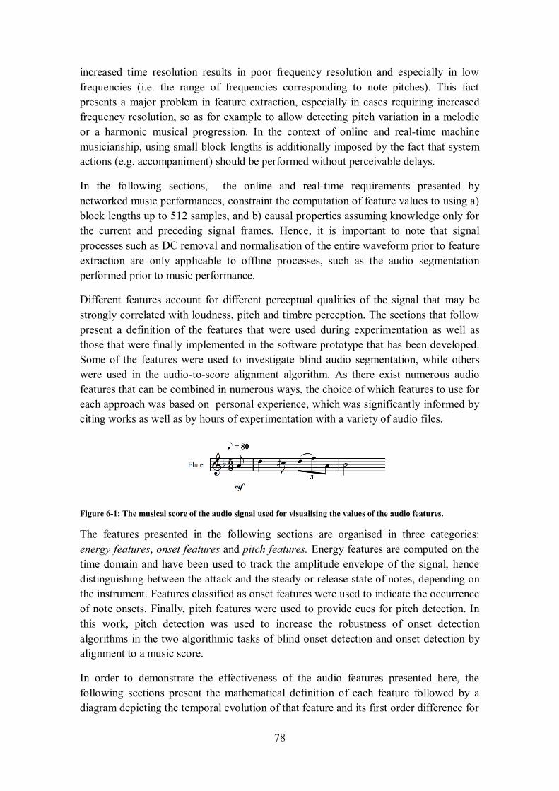
78
increased time resolution results in poor frequency resolution and especially in low
frequencies (i.e. the range of frequencies corresponding to note pitches). This fact
presents a major problem in feature extraction, especially in cases requiring increased
frequency resolution, so as for example to allow detecting pitch variation in a melodic
or a harmonic musical progression. In the context of online and real-time machine
musicianship, using small block lengths is additionally imposed by the fact that system
actions (e.g. accompaniment) should be performed without perceivable delays.
In the following sections, the online and real-time requirements presented by
networked music performances, constraint the computation of feature values to using a)
block lengths up to 512 samples, and b) causal properties assuming knowledge only for
the current and preceding signal frames. Hence, it is important to note that signal
processes such as DC removal and normalisation of the entire waveform prior to feature
extraction are only applicable to offline processes, such as the audio segmentation
performed prior to music performance.
Different features account for different perceptual qualities of the signal that may be
strongly correlated with loudness, pitch and timbre perception. The sections that follow
present a definition of the features that were used during experimentation as well as
those that were finally implemented in the software prototype that has been developed.
Some of the features were used to investigate blind audio segmentation, while others
were used in the audio-to-score alignment algorithm. As there exist numerous audio
features that can be combined in numerous ways, the choice of which features to use for
each approach was based on personal experience, which was significantly informed by
citing works as well as by hours of experimentation with a variety of audio files.
Figure 6-1: The musical score of the audio signal used for visualising the values of the audio features.
The features presented in the following sections are organised in three categories:
energy features, onset features and pitch features. Energy features are computed on the
time domain and have been used to track the amplitude envelope of the signal, hence
distinguishing between the attack and the steady or release state of notes, depending on
the instrument. Features classified as onset features were used to indicate the occurrence
of note onsets. Finally, pitch features were used to provide cues for pitch detection. In
this work, pitch detection was used to increase the robustness of onset detection
algorithms in the two algorithmic tasks of blind onset detection and onset detection by
alignment to a music score.
In order to demonstrate the effectiveness of the audio features presented here, the
following sections present the mathematical definition of each feature followed by a
diagram depicting the temporal evolution of that feature and its first order difference for
79
an example melodic phrase. The signal is a flute performance of the melody shown on
Figure 6-1. The fifth note is performed as a subtle pitch change, i.e. a legato articulation.
The signal has a total duration of 4.12sec and the features have been estimated on audio
blocks having a length of 11.6ms (i.e. 512 samples of 44100/16bit audio).
6.2 Mathematical notation
The definition of features in the next sections, comply with the following mathematical
notation:
: denotes the length of the audio block
: denotes the sample index within an audio block
: denotes the block index starting from 0
: denotes the number of frequency bins in the spectrum up to the Nyquist
frequency
: denotes the index of frequency bins
: denotes the signal value at time instant t
: denotes the kth frequency bin of the complex Fourier spectrum of the n
th
audio block
: denotes the spectral magnitude of the kth
frequency bin of the nth
block
: denotes the phase of the kth frequency bin of the signal at block n
: denotes the value of feature F at block n
: denotes the first order difference of feature F at
block n
: denotes the second order difference of feature
F at block n.
The last two differences values (the equivalent of the first and the second derivative in
analogue signals) are often used in combination with the actual feature value, so as to
allow monitoring the monotonicity of the corresponding features along with their local
values.
6.3 A note on frequency transforms
This section discusses the importance of proper parameterisation of the Fourier
transform for the proposed application scenario on NMP. The Fourier transform is used
to compute spectral features, which are monitored in real-time in order to indicate the
occurrence of note onsets. For the application scenario addressed here, it is important to
realize that note onsets need to be detected as soon as they occur. This requirement is
imposed by the fact following the detection of an onset, a notification will be
transmitted to all remote network ends and re-synthesis of the corresponding note
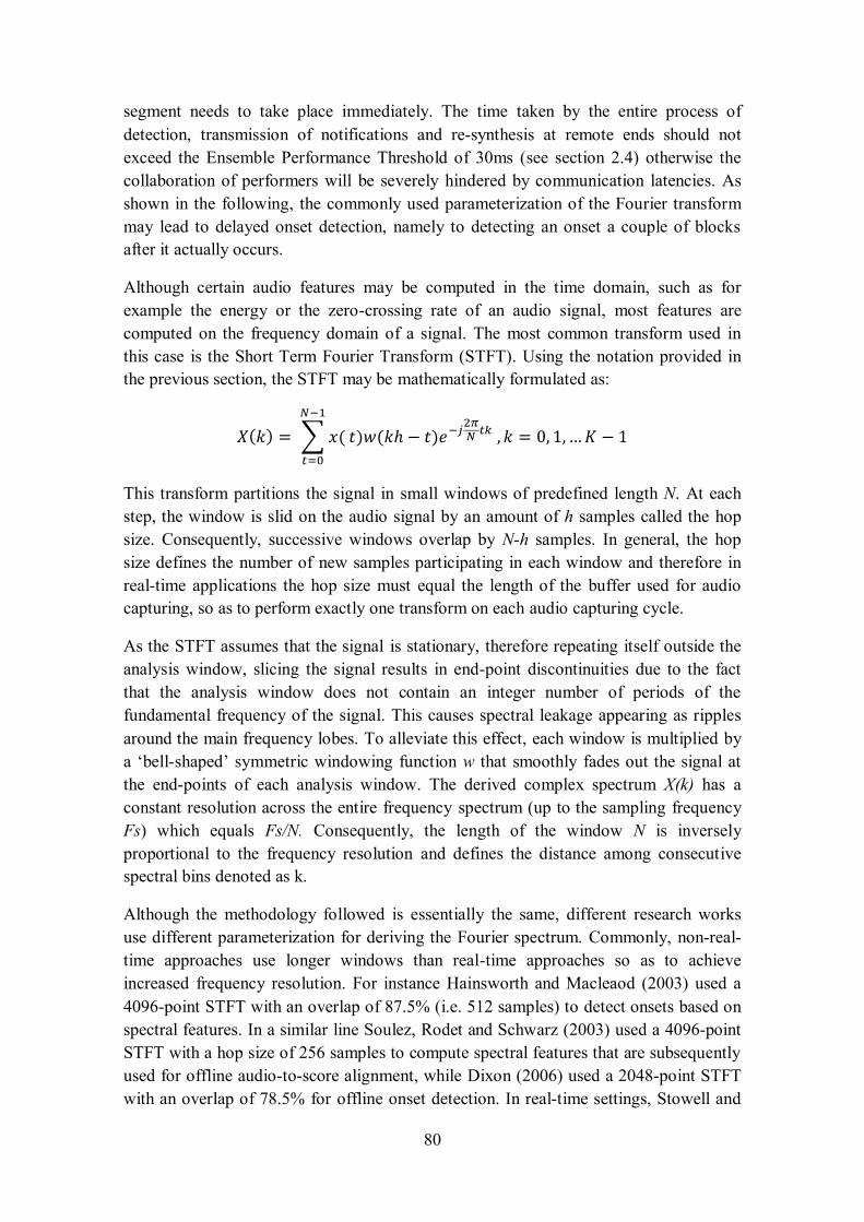
80
segment needs to take place immediately. The time taken by the entire process of
detection, transmission of notifications and re-synthesis at remote ends should not
exceed the Ensemble Performance Threshold of 30ms (see section 2.4) otherwise the
collaboration of performers will be severely hindered by communication latencies. As
shown in the following, the commonly used parameterization of the Fourier transform
may lead to delayed onset detection, namely to detecting an onset a couple of blocks
after it actually occurs.
Although certain audio features may be computed in the time domain, such as for
example the energy or the zero-crossing rate of an audio signal, most features are
computed on the frequency domain of a signal. The most common transform used in
this case is the Short Term Fourier Transform (STFT). Using the notation provided in
the previous section, the STFT may be mathematically formulated as:
This transform partitions the signal in small windows of predefined length N. At each
step, the window is slid on the audio signal by an amount of h samples called the hop
size. Consequently, successive windows overlap by N-h samples. In general, the hop
size defines the number of new samples participating in each window and therefore in
real-time applications the hop size must equal the length of the buffer used for audio
capturing, so as to perform exactly one transform on each audio capturing cycle.
As the STFT assumes that the signal is stationary, therefore repeating itself outside the
analysis window, slicing the signal results in end-point discontinuities due to the fact
that the analysis window does not contain an integer number of periods of the
fundamental frequency of the signal. This causes spectral leakage appearing as ripples
around the main frequency lobes. To alleviate this effect, each window is multiplied by
a ‘bell-shaped’ symmetric windowing function w that smoothly fades out the signal at
the end-points of each analysis window. The derived complex spectrum X(k) has a
constant resolution across the entire frequency spectrum (up to the sampling frequency
Fs) which equals Fs/N. Consequently, the length of the window N is inversely
proportional to the frequency resolution and defines the distance among consecutive
spectral bins denoted as k.
Although the methodology followed is essentially the same, different research works
use different parameterization for deriving the Fourier spectrum. Commonly, non-real-
time approaches use longer windows than real-time approaches so as to achieve
increased frequency resolution. For instance Hainsworth and Macleaod (2003) used a
4096-point STFT with an overlap of 87.5% (i.e. 512 samples) to detect onsets based on
spectral features. In a similar line Soulez, Rodet and Schwarz (2003) used a 4096-point
STFT with a hop size of 256 samples to compute spectral features that are subsequently
used for offline audio-to-score alignment, while Dixon (2006) used a 2048-point STFT
with an overlap of 78.5% for offline onset detection. In real-time settings, Stowell and
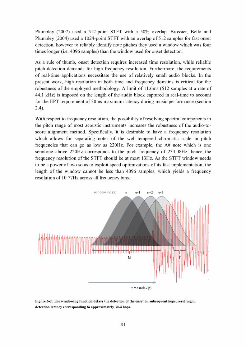
81
Plumbley (2007) used a 512-point STFT with a 50% overlap. Brossier, Bello and
Plumbley (2004) used a 1024-point STFT with an overlap of 512 samples for fast onset
detection, however to reliably identify note pitches they used a window which was four
times longer (i.e. 4096 samples) than the window used for onset detection.
As a rule of thumb, onset detection requires increased time resolution, while reliable
pitch detection demands for high frequency resolution. Furthermore, the requirements
of real-time applications necessitate the use of relatively small audio blocks. In the
present work, high resolution in both time and frequency domains is critical for the
robustness of the employed methodology. A limit of 11.6ms (512 samples at a rate of
44.1 kHz) is imposed on the length of the audio block captured in real-time to account
for the EPT requirement of 30ms maximum latency during music performance (section
2.4).
With respect to frequency resolution, the possibility of resolving spectral components in
the pitch range of most acoustic instruments increases the robustness of the audio-to-
score alignment method. Specifically, it is desirable to have a frequency resolution
which allows for separating notes of the well-tempered chromatic scale in pitch
frequencies that can go as low as 220Hz. For example, the A# note which is one
semitone above 220Hz corresponds to the pitch frequency of 233,08Hz, hence the
frequency resolution of the STFT should be at most 13Hz. As the STFT window needs
to be a power of two so as to exploit speed optimizations of its fast implementation, the
length of the window cannot be less than 4096 samples, which yields a frequency
resolution of 10.77Hz across all frequency bins.
Figure 6-2: The windowing function delays the detection of the onset on subsequent hops, resulting in
detection latency corresponding to approximately 30-4 hops.
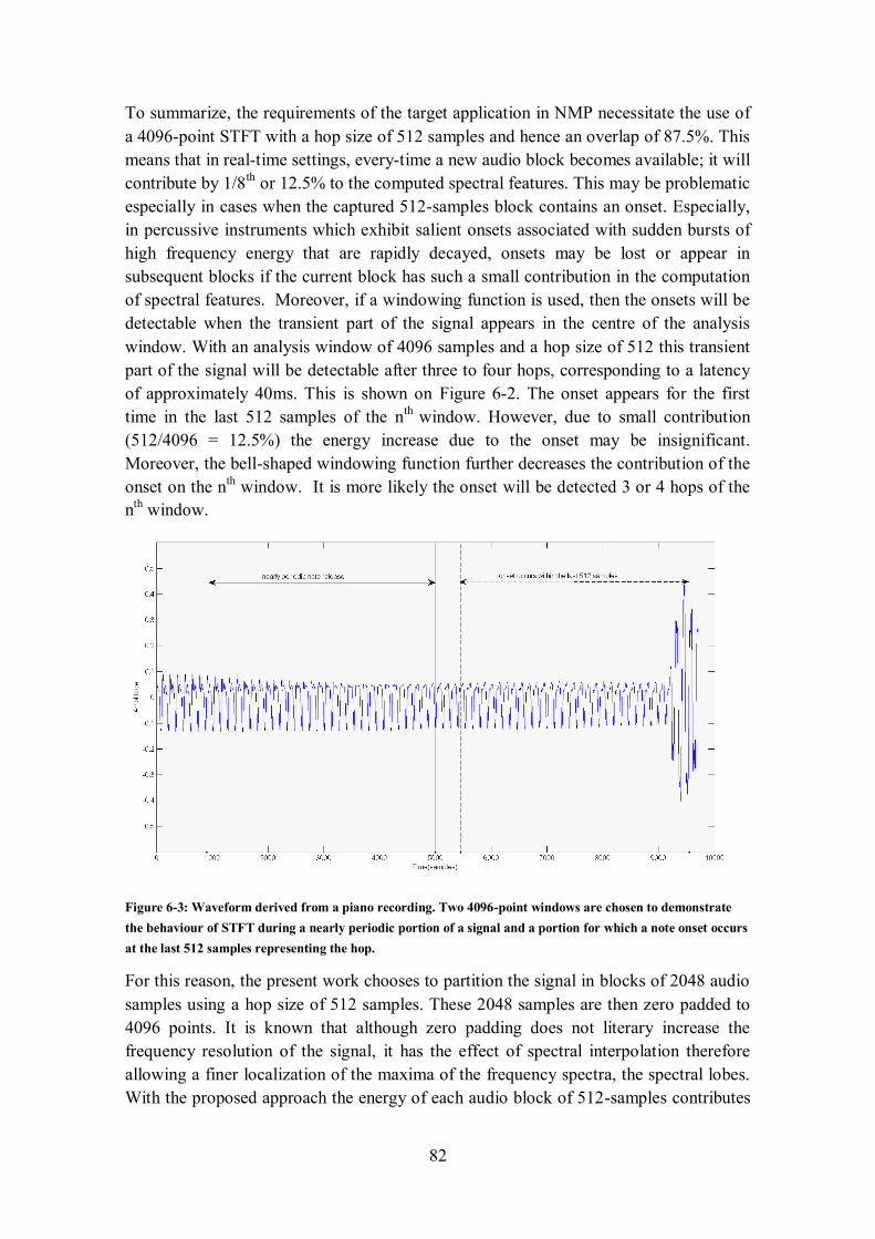
82
To summarize, the requirements of the target application in NMP necessitate the use of
a 4096-point STFT with a hop size of 512 samples and hence an overlap of 87.5%. This
means that in real-time settings, every-time a new audio block becomes available; it will
contribute by 1/8th
or 12.5% to the computed spectral features. This may be problematic
especially in cases when the captured 512-samples block contains an onset. Especially,
in percussive instruments which exhibit salient onsets associated with sudden bursts of
high frequency energy that are rapidly decayed, onsets may be lost or appear in
subsequent blocks if the current block has such a small contribution in the computation
of spectral features. Moreover, if a windowing function is used, then the onsets will be
detectable when the transient part of the signal appears in the centre of the analysis
window. With an analysis window of 4096 samples and a hop size of 512 this transient
part of the signal will be detectable after three to four hops, corresponding to a latency
of approximately 40ms. This is shown on Figure 6-2. The onset appears for the first
time in the last 512 samples of the nth
window. However, due to small contribution
(512/4096 = 12.5%) the energy increase due to the onset may be insignificant.
Moreover, the bell-shaped windowing function further decreases the contribution of the
onset on the nth window. It is more likely the onset will be detected 3 or 4 hops of the
nth
window.
Figure 6-3: Waveform derived from a piano recording. Two 4096-point windows are chosen to demonstrate
the behaviour of STFT during a nearly periodic portion of a signal and a portion for which a note onset occurs
at the last 512 samples representing the hop.
For this reason, the present work chooses to partition the signal in blocks of 2048 audio
samples using a hop size of 512 samples. These 2048 samples are then zero padded to
4096 points. It is known that although zero padding does not literary increase the
frequency resolution of the signal, it has the effect of spectral interpolation therefore
allowing a finer localization of the maxima of the frequency spectra, the spectral lobes.
With the proposed approach the energy of each audio block of 512-samples contributes
83
by 25% to the computed spectral features, which provides a good compromise between
time and frequency resolution. Moreover, the windowing function w(n) corresponds to a
rectangular window which is equivalent to not using a windowing function.
The superiority of the proposed transform over the conventional STFT for the task of
onset detection is demonstrated using an example audio signal. The signal shown on
Figure 6-3 has been derived from a piano recording playing a monophonic tune.
Specifically, two 4096-point windows have been chosen: the first one is derived from
the steady, nearly periodic, part of a note and the second one contains the onset of the
next note within the last hop of 512 samples. For the computation of the STFT a
Hanning windowing function has been used, which is mathematically formulated as:
where N equals the number of samples used in the analysis window. Four
parameterisations of the STFT have been chosen for demonstration:
1. 512-point STFT using a Hanning window
2. 4096-point STFT using a Hanning window
3. 2048-point STFT using a Hanning window of 2048-points (i.e. N = 2048) and a
Fourier analysis window which is zero padded to 4096
4. 2048-point STFT using a rectangular windowing function (i.e. which is
equivalent to no windowing function) and a Fourier analysis window which is
zero padded to 4096
Figure 6-4 shows the frequency spectra of the periodic part of the signal derived using
the above parameterisations, while Figure 6-5 contains the same plot but with the
transforms applied on the window that contains an onset during the last 512 samples.
Note that the first parameterisation of the Fourier transform is applied on the last 512
samples of the window, the second on the entire window while the third and the fourth
parameterisations are applied on the second half (i.e. the last 2048 samples) of each
window.
The following conclusions may be drawn from these spectra:
Window Size and Frequency Resolution: The 512 transform (1) has a very
coarse frequency resolution, hindering the separation of pitches in the task of
audio to score alignment. The remaining parameterisations give a better estimate
of the main spectral lobe (in this case corresponding to the fundamental
frequency) as well as the next three harmonics.
Window Shape and Spectral Leakage: The use of the rectangular window in the
fourth parameterisation (4), introduces ripples around the main spectral lobes,
which is caused by spectral leakage introduced by signal discontinuities at the
end points of the analysis window. This effect is suppressed when using a
84
Hanning window that smoothly fades out the signal at the end points of the
analysis window.
Zero Padding vs. Not Zero Padding: The 2048 signal zero padded to form a
4096 point analysis window (3) yields an identical spectral shape to the 4096
point STFT (2) which however contains less energy, due to fewer samples with
non-zero amplitude. Mere zero-padding does not appear to significantly
contribute to early onset detection.
Periodicity and divergence: The most important conclusion drawn from these
two diagrams is that both the 4096 Hanning STFT (2) as well as the 2048
Hanning STFT (3) parameterisations have a very similar spectrum in the two
signal regions, therefore providing no hint for the occurrence of the onset on the
last 512 samples of the second spectrum. In both cases, the onset is attenuated
by the Hanning windowing function. In contrast, the 2048 STFT using a
rectangular window (4), provides a very different spectrum in the two figures,
which contains a substantial percentage of energy in higher frequencies as well
as in frequencies between the main lobes, thus clearly indicating the occurrence
of the onset. In the periodic part of the signal it has a spectrum which is very
close to the 4096 Hanning STFT (2), therefore clearly depicting that the signal is
highly periodic. It can also be seen that the 512 parameterisation (1) yields a
spectrum of higher energy than that of the periodic part of the spectrum. This
energy increase may also be used to inform onset detection. However, as the
present application additionally uses pitch identification to increase the
robustness of audio to score alignment, the last parameterisation (4) yields better
results both for onset detection as well as for audio to score alignment. It can be
argued that the same performance may be achieved by using a rectangular
window on 4096 samples, thus omitting zero padded. However, as previously
discussed, using 2048 samples is preferred due to each 512-hop having a greater
contribution to the resulting spectrum, i.e. twice than that without zero padding.
All of the algorithms presented in the rest of this dissertation use an STFT applied on
analysis windows for which the first 2048 points are audio samples and the second half
is zero padded. Out of the 2048 samples, 512 correspond to the audio block captured in
real-time (i.e. yielding a 75% overlap factor). No windowing function is used in order to
avoid eliminating transient phenomena at the time of their occurrence. Experiments on a
number of acoustic instruments confirmed that this parameterisation offers a good
compromise between timely identification of note onsets and frequency resolution to
allowing distinguishing note pitches in the frequency range of interest.
The spectral features defined and visualised in the sections that follow are computed
using the proposed parameterisation of the Fourier transform. The rest of the features,
namely those computed on the time domain (i.e. E, RMS, LE) and the WP feature
(which uses a Discrete Wavelet Transform instead of the Fourier transform) are
computed on consecutive 512-sample blocks.
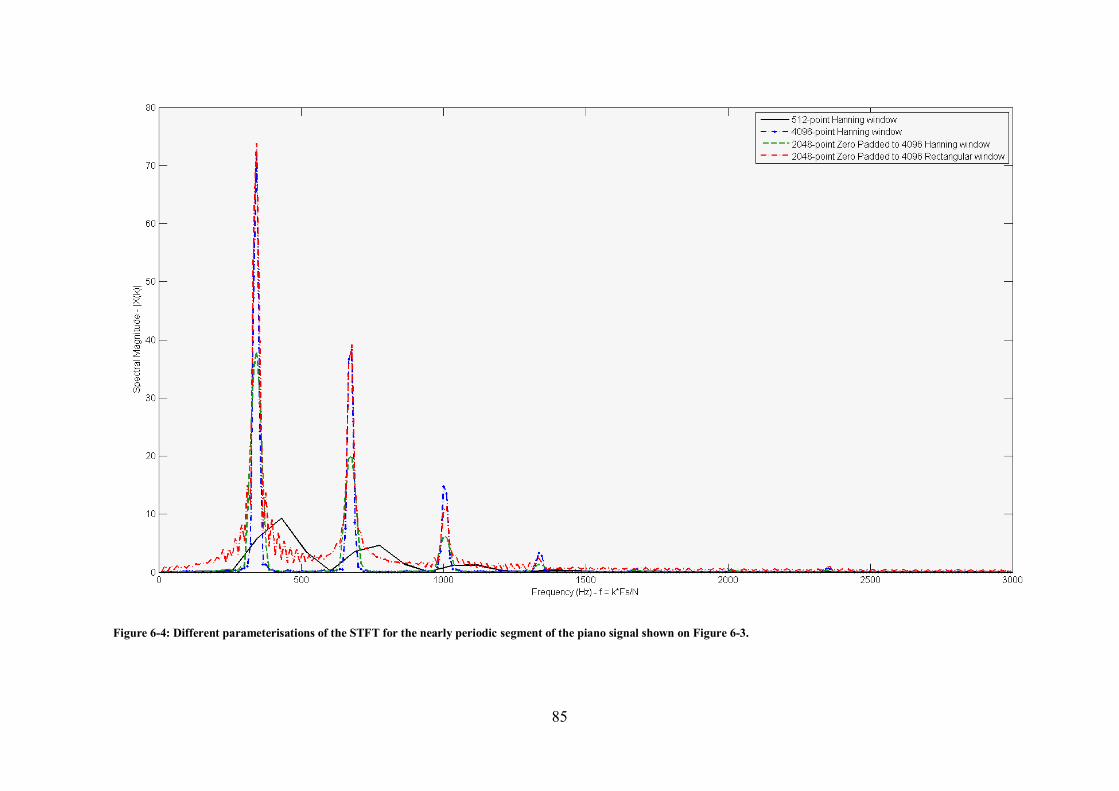
85
Figure 6-4: Different parameterisations of the STFT for the nearly periodic segment of the piano signal shown on Figure 6-3.
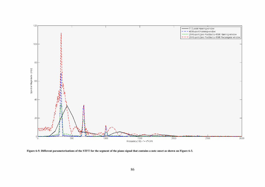
86
Figure 6-5: Different parameterisations of the STFT for the segment of the piano signal that contains a note onset as shown on Figure 6-3.
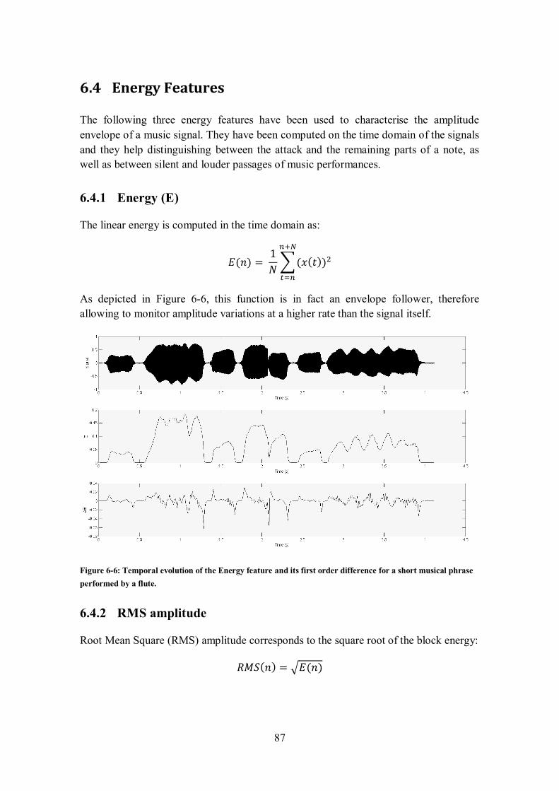
87
6.4 Energy Features
The following three energy features have been used to characterise the amplitude
envelope of a music signal. They have been computed on the time domain of the signals
and they help distinguishing between the attack and the remaining parts of a note, as
well as between silent and louder passages of music performances.
6.4.1 Energy (E)
The linear energy is computed in the time domain as:
As depicted in Figure 6-6, this function is in fact an envelope follower, therefore
allowing to monitor amplitude variations at a higher rate than the signal itself.
Figure 6-6: Temporal evolution of the Energy feature and its first order difference for a short musical phrase
performed by a flute.
6.4.2 RMS amplitude
Root Mean Square (RMS) amplitude corresponds to the square root of the block energy:
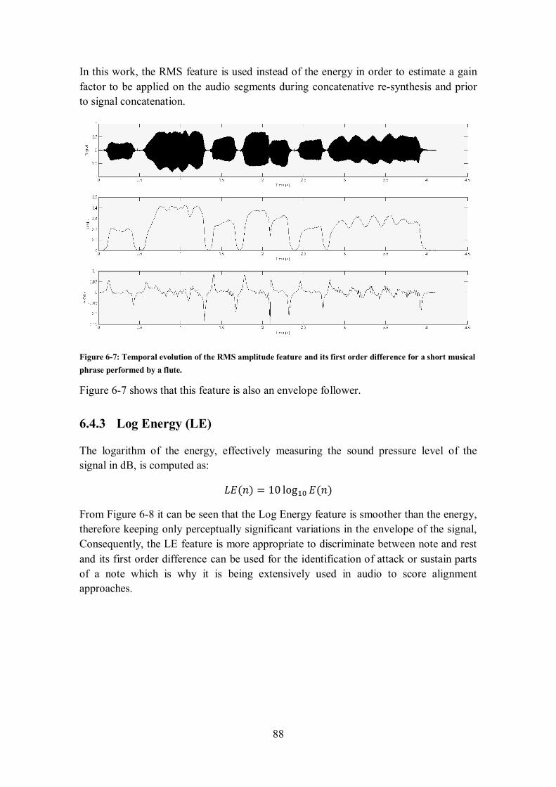
88
In this work, the RMS feature is used instead of the energy in order to estimate a gain
factor to be applied on the audio segments during concatenative re-synthesis and prior
to signal concatenation.
Figure 6-7: Temporal evolution of the RMS amplitude feature and its first order difference for a short musical
phrase performed by a flute.
Figure 6-7 shows that this feature is also an envelope follower.
6.4.3 Log Energy (LE)
The logarithm of the energy, effectively measuring the sound pressure level of the
signal in dB, is computed as:
From Figure 6-8 it can be seen that the Log Energy feature is smoother than the energy,
therefore keeping only perceptually significant variations in the envelope of the signal,
Consequently, the LE feature is more appropriate to discriminate between note and rest
and its first order difference can be used for the identification of attack or sustain parts
of a note which is why it is being extensively used in audio to score alignment
approaches.
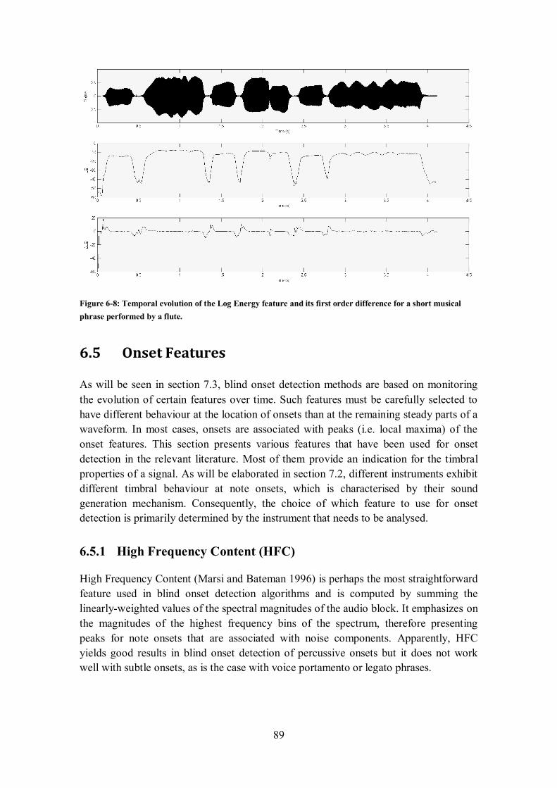
89
Figure 6-8: Temporal evolution of the Log Energy feature and its first order difference for a short musical
phrase performed by a flute.
6.5 Onset Features
As will be seen in section 7.3, blind onset detection methods are based on monitoring
the evolution of certain features over time. Such features must be carefully selected to
have different behaviour at the location of onsets than at the remaining steady parts of a
waveform. In most cases, onsets are associated with peaks (i.e. local maxima) of the
onset features. This section presents various features that have been used for onset
detection in the relevant literature. Most of them provide an indication for the timbral
properties of a signal. As will be elaborated in section 7.2, different instruments exhibit
different timbral behaviour at note onsets, which is characterised by their sound
generation mechanism. Consequently, the choice of which feature to use for onset
detection is primarily determined by the instrument that needs to be analysed.
6.5.1 High Frequency Content (HFC)
High Frequency Content (Marsi and Bateman 1996) is perhaps the most straightforward
feature used in blind onset detection algorithms and is computed by summing the
linearly-weighted values of the spectral magnitudes of the audio block. It emphasizes on
the magnitudes of the highest frequency bins of the spectrum, therefore presenting
peaks for note onsets that are associated with noise components. Apparently, HFC
yields good results in blind onset detection of percussive onsets but it does not work
well with subtle onsets, as is the case with voice portamento or legato phrases.
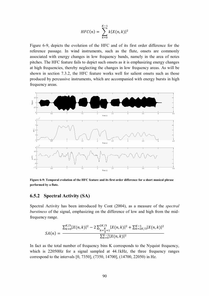
90
Figure 6-9, depicts the evolution of the HFC and of its first order difference for the
reference passage. In wind instruments, such as the flute, onsets are commonly
associated with energy changes in low frequency bands, namely in the area of notes
pitches. The HFC feature fails to depict such onsets as it is emphasizing energy changes
at high frequencies, thereby neglecting the changes in low frequency areas. As will be
shown in section 7.3.2, the HFC feature works well for salient onsets such as those
produced by percussive instruments, which are accompanied with energy bursts in high
frequency areas.
Figure 6-9: Temporal evolution of the HFC feature and its first order difference for a short musical phrase
performed by a flute.
6.5.2 Spectral Activity (SA)
Spectral Activity has been introduced by Cont (2004), as a measure of the spectral
burstiness of the signal, emphasizing on the difference of low and high from the mid-
frequency range.
In fact as the total number of frequency bins K corresponds to the Nyquist frequency,
which is 22050Hz for a signal sampled at 44.1kHz, the three frequency ranges
correspond to the intervals [0, 7350], (7350, 14700], (14700, 22050) in Hz.
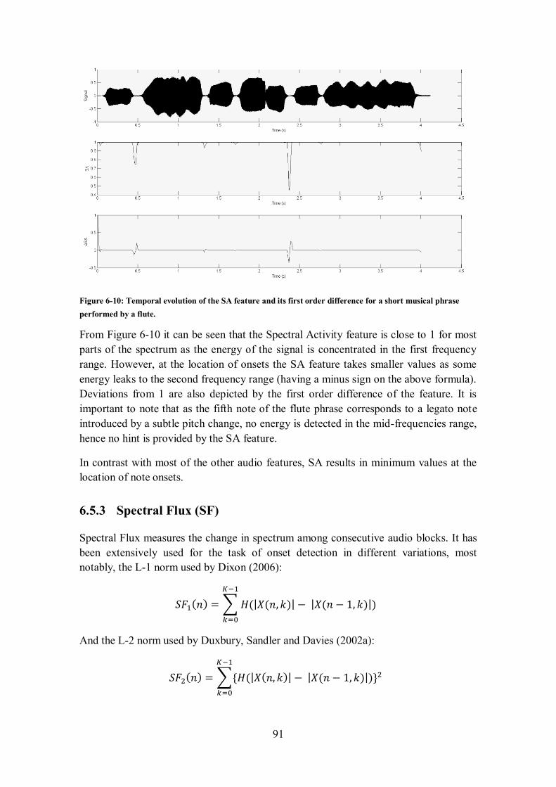
91
Figure 6-10: Temporal evolution of the SA feature and its first order difference for a short musical phrase
performed by a flute.
From Figure 6-10 it can be seen that the Spectral Activity feature is close to 1 for most
parts of the spectrum as the energy of the signal is concentrated in the first frequency
range. However, at the location of onsets the SA feature takes smaller values as some
energy leaks to the second frequency range (having a minus sign on the above formula).
Deviations from 1 are also depicted by the first order difference of the feature. It is
important to note that as the fifth note of the flute phrase corresponds to a legato note
introduced by a subtle pitch change, no energy is detected in the mid-frequencies range,
hence no hint is provided by the SA feature.
In contrast with most of the other audio features, SA results in minimum values at the
location of note onsets.
6.5.3 Spectral Flux (SF)
Spectral Flux measures the change in spectrum among consecutive audio blocks. It has
been extensively used for the task of onset detection in different variations, most
notably, the L-1 norm used by Dixon (2006):
And the L-2 norm used by Duxbury, Sandler and Davies (2002a):
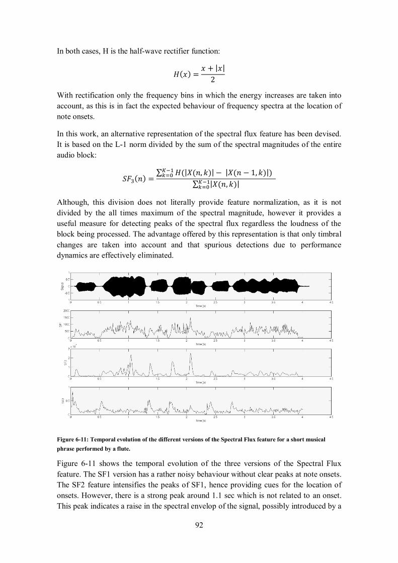
92
In both cases, H is the half-wave rectifier function:
With rectification only the frequency bins in which the energy increases are taken into
account, as this is in fact the expected behaviour of frequency spectra at the location of
note onsets.
In this work, an alternative representation of the spectral flux feature has been devised.
It is based on the L-1 norm divided by the sum of the spectral magnitudes of the entire
audio block:
Although, this division does not literally provide feature normalization, as it is not
divided by the all times maximum of the spectral magnitude, however it provides a
useful measure for detecting peaks of the spectral flux regardless the loudness of the
block being processed. The advantage offered by this representation is that only timbral
changes are taken into account and that spurious detections due to performance
dynamics are effectively eliminated.
Figure 6-11: Temporal evolution of the different versions of the Spectral Flux feature for a short musical
phrase performed by a flute.
Figure 6-11 shows the temporal evolution of the three versions of the Spectral Flux
feature. The SF1 version has a rather noisy behaviour without clear peaks at note onsets.
The SF2 feature intensifies the peaks of SF1, hence providing cues for the location of
onsets. However, there is a strong peak around 1.1 sec which is not related to an onset.
This peak indicates a raise in the spectral envelop of the signal, possibly introduced by a
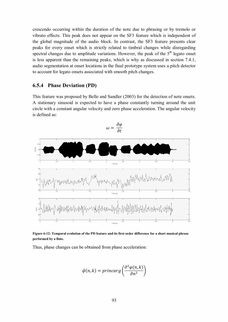
93
crescendo occurring within the duration of the note due to phrasing or by tremolo or
vibrato effects. This peak does not appear on the SF3 feature which is independent of
the global magnitude of the audio block. In contrast, the SF3 feature presents clear
peaks for every onset which is strictly related to timbral changes while disregarding
spectral changes due to amplitude variations. However, the peak of the 5th legato onset
is less apparent than the remaining peaks, which is why as discussed in section 7.4.1,
audio segmentation at onset locations in the final prototype system uses a pitch detector
to account for legato onsets associated with smooth pitch changes.
6.5.4 Phase Deviation (PD)
This feature was proposed by Bello and Sandler (2003) for the detection of note onsets.
A stationary sinusoid is expected to have a phase constantly turning around the unit
circle with a constant angular velocity and zero phase acceleration. The angular velocity
is defined as:
Figure 6-12: Temporal evolution of the PD feature and its first order difference for a short musical phrase
performed by a flute.
Thus, phase changes can be obtained from phase acceleration:
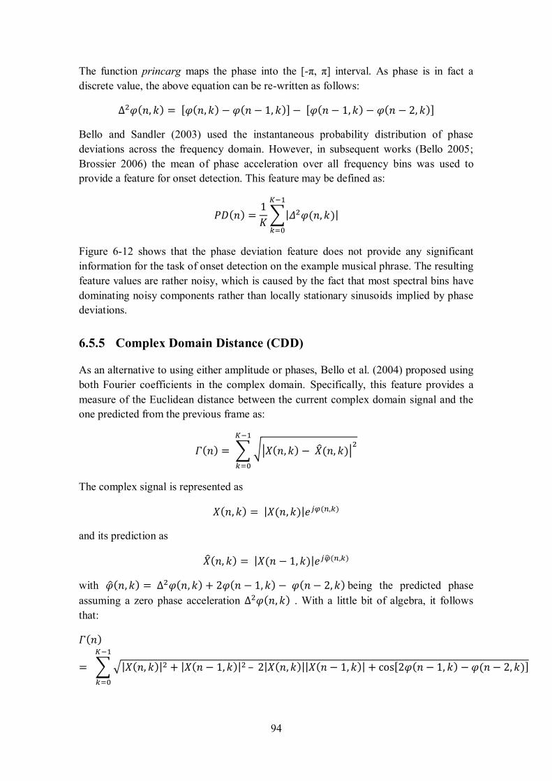
94
The function princarg maps the phase into the [-π, π] interval. As phase is in fact a
discrete value, the above equation can be re-written as follows:
Bello and Sandler (2003) used the instantaneous probability distribution of phase
deviations across the frequency domain. However, in subsequent works (Bello 2005;
Brossier 2006) the mean of phase acceleration over all frequency bins was used to
provide a feature for onset detection. This feature may be defined as:
Figure 6-12 shows that the phase deviation feature does not provide any significant
information for the task of onset detection on the example musical phrase. The resulting
feature values are rather noisy, which is caused by the fact that most spectral bins have
dominating noisy components rather than locally stationary sinusoids implied by phase
deviations.
6.5.5 Complex Domain Distance (CDD)
As an alternative to using either amplitude or phases, Bello et al. (2004) proposed using
both Fourier coefficients in the complex domain. Specifically, this feature provides a
measure of the Euclidean distance between the current complex domain signal and the
one predicted from the previous frame as:
The complex signal is represented as
and its prediction as
with being the predicted phase
assuming a zero phase acceleration . With a little bit of algebra, it follows
that:
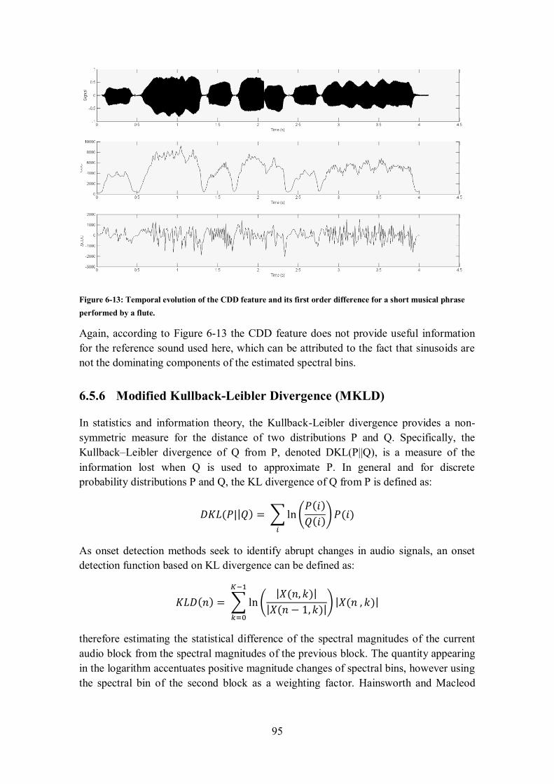
95
Figure 6-13: Temporal evolution of the CDD feature and its first order difference for a short musical phrase
performed by a flute.
Again, according to Figure 6-13 the CDD feature does not provide useful information
for the reference sound used here, which can be attributed to the fact that sinusoids are
not the dominating components of the estimated spectral bins.
6.5.6 Modified Kullback-Leibler Divergence (MKLD)
In statistics and information theory, the Kullback-Leibler divergence provides a non-
symmetric measure for the distance of two distributions P and Q. Specifically, the
Kullback–Leibler divergence of Q from P, denoted DKL(P||Q), is a measure of the
information lost when Q is used to approximate P. In general and for discrete
probability distributions P and Q, the KL divergence of Q from P is defined as:
As onset detection methods seek to identify abrupt changes in audio signals, an onset
detection function based on KL divergence can be defined as:
therefore estimating the statistical difference of the spectral magnitudes of the current
audio block from the spectral magnitudes of the previous block. The quantity appearing
in the logarithm accentuates positive magnitude changes of spectral bins, however using
the spectral bin of the second block as a weighting factor. Hainsworth and Macleod
96
(2003) proposed removing the weighting factor, thereby simply reflecting the rate of
positive amplitude evolution between successive blocks:
Based on this measure, Brossier (2006) proposed a modified version formulated as:
which firstly prevents negative values and introduces the term ε=10-6
to ensure that the
feature is still defined in very low energy levels approaching zero.
Figure 6-14: Temporal evolution of the MKL feature and its first order difference for a short musical phrase
performed by a flute.
As will be seen in section 7.3.2, the MKL feature is highly effective for percussive
onset detection. Unfortunately, as shown on Figure 6-14 it does not effectively depict
onsets for non-percussive sounds, as it appears that the variation of spectral envelopes at
onset locations is not significantly different than at the remaining parts of the signal.
6.6 Pitch Features
The prototype system developed in this work uses two audio features related to pitch.
These are the pitch values determined using a discrete wavelet transform and the PSM
feature, which is based on the Fourier transform and provides a measure for the
presence of a given pitch in the audio block over which it is computed.
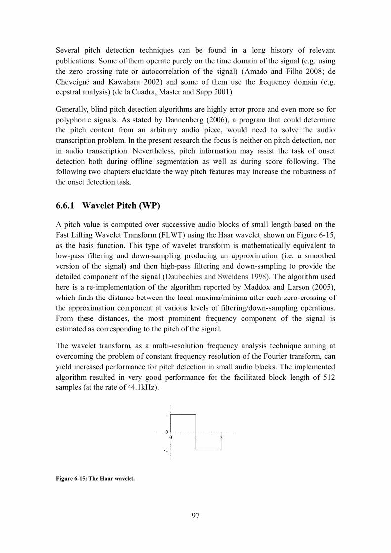
97
Several pitch detection techniques can be found in a long history of relevant
publications. Some of them operate purely on the time domain of the signal (e.g. using
the zero crossing rate or autocorrelation of the signal) (Amado and Filho 2008; de
Cheveigné and awahara 2002) and some of them use the frequency domain (e.g.
cepstral analysis) (de la Cuadra, Master and Sapp 2001)
Generally, blind pitch detection algorithms are highly error prone and even more so for
polyphonic signals. As stated by Dannenberg (2006), a program that could determine
the pitch content from an arbitrary audio piece, would need to solve the audio
transcription problem. In the present research the focus is neither on pitch detection, nor
in audio transcription. Nevertheless, pitch information may assist the task of onset
detection both during offline segmentation as well as during score following. The
following two chapters elucidate the way pitch features may increase the robustness of
the onset detection task.
6.6.1 Wavelet Pitch (WP)
A pitch value is computed over successive audio blocks of small length based on the
Fast Lifting Wavelet Transform (FLWT) using the Haar wavelet, shown on Figure 6-15,
as the basis function. This type of wavelet transform is mathematically equivalent to
low-pass filtering and down-sampling producing an approximation (i.e. a smoothed
version of the signal) and then high-pass filtering and down-sampling to provide the
detailed component of the signal (Daubechies and Sweldens 1998). The algorithm used
here is a re-implementation of the algorithm reported by Maddox and Larson (2005),
which finds the distance between the local maxima/minima after each zero-crossing of
the approximation component at various levels of filtering/down-sampling operations.
From these distances, the most prominent frequency component of the signal is
estimated as corresponding to the pitch of the signal.
The wavelet transform, as a multi-resolution frequency analysis technique aiming at
overcoming the problem of constant frequency resolution of the Fourier transform, can
yield increased performance for pitch detection in small audio blocks. The implemented
algorithm resulted in very good performance for the facilitated block length of 512
samples (at the rate of 44.1kHz).
Figure 6-15: The Haar wavelet.
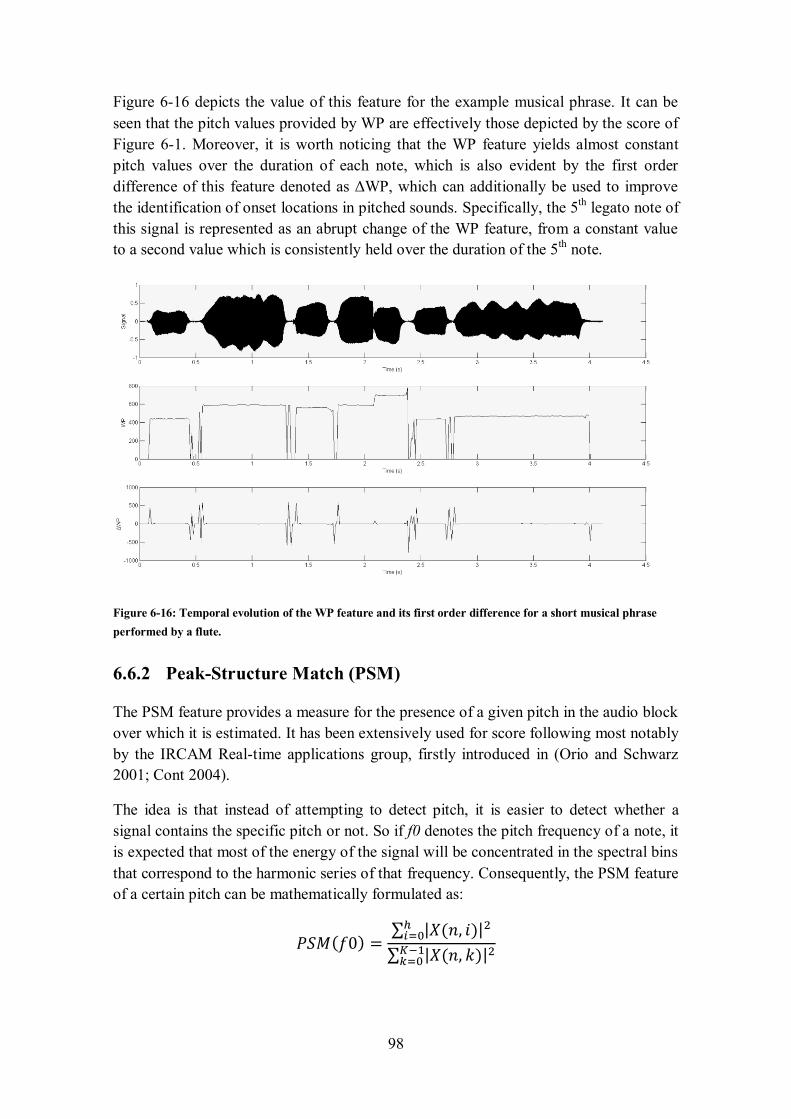
98
Figure 6-16 depicts the value of this feature for the example musical phrase. It can be
seen that the pitch values provided by WP are effectively those depicted by the score of
Figure 6-1. Moreover, it is worth noticing that the WP feature yields almost constant
pitch values over the duration of each note, which is also evident by the first order
difference of this feature denoted as ΔWP, which can additionally be used to improve
the identification of onset locations in pitched sounds. Specifically, the 5th
legato note of
this signal is represented as an abrupt change of the WP feature, from a constant value
to a second value which is consistently held over the duration of the 5th note.
Figure 6-16: Temporal evolution of the WP feature and its first order difference for a short musical phrase
performed by a flute.
6.6.2 Peak-Structure Match (PSM)
The PSM feature provides a measure for the presence of a given pitch in the audio block
over which it is estimated. It has been extensively used for score following most notably
by the IRCAM Real-time applications group, firstly introduced in (Orio and Schwarz
2001; Cont 2004).
The idea is that instead of attempting to detect pitch, it is easier to detect whether a
signal contains the specific pitch or not. So if f0 denotes the pitch frequency of a note, it
is expected that most of the energy of the signal will be concentrated in the spectral bins
that correspond to the harmonic series of that frequency. Consequently, the PSM feature
of a certain pitch can be mathematically formulated as:
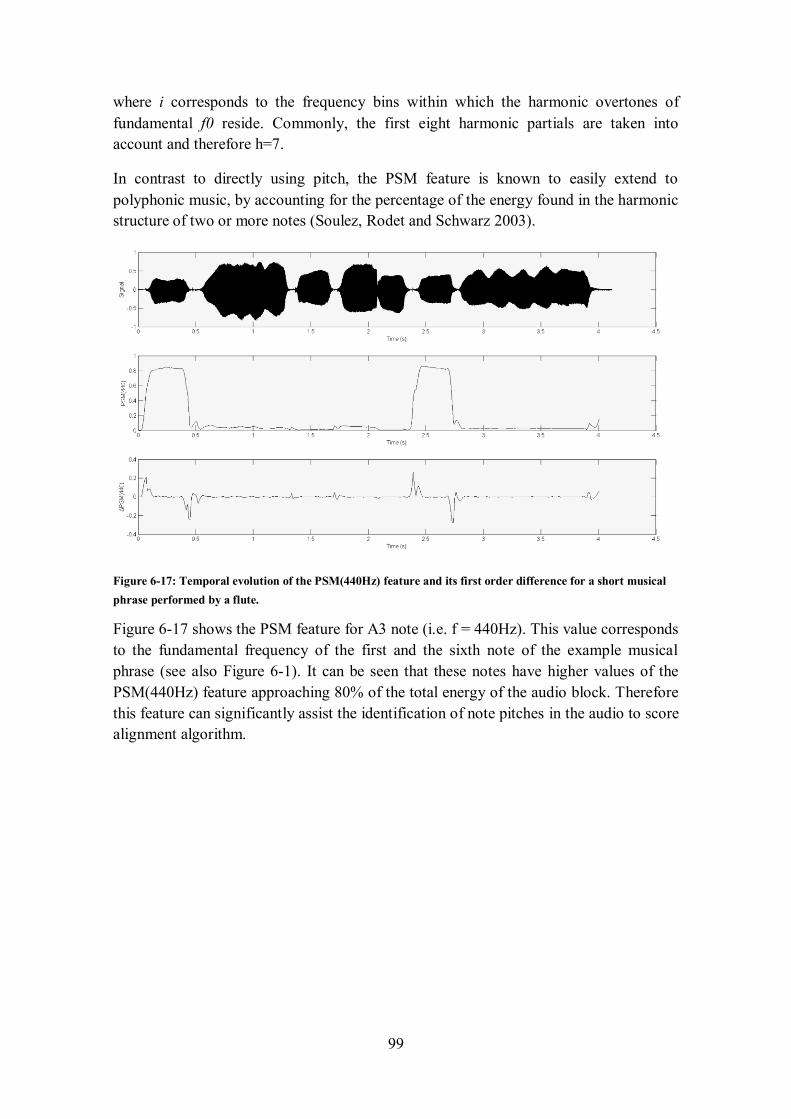
99
where i corresponds to the frequency bins within which the harmonic overtones of
fundamental f0 reside. Commonly, the first eight harmonic partials are taken into
account and therefore h=7.
In contrast to directly using pitch, the PSM feature is known to easily extend to
polyphonic music, by accounting for the percentage of the energy found in the harmonic
structure of two or more notes (Soulez, Rodet and Schwarz 2003).
Figure 6-17: Temporal evolution of the PSM(440Hz) feature and its first order difference for a short musical
phrase performed by a flute.
Figure 6-17 shows the PSM feature for A3 note (i.e. f = 440Hz). This value corresponds
to the fundamental frequency of the first and the sixth note of the example musical
phrase (see also Figure 6-1). It can be seen that these notes have higher values of the
PSM(440Hz) feature approaching 80% of the total energy of the audio block. Therefore
this feature can significantly assist the identification of note pitches in the audio to score
alignment algorithm.
100
7 Offline Audio Segmentation
This chapter presents the methodology that was adopted for segmenting the solo
recording of each musician in the target prototype system. The resulting segments are
needed during live performance to remotely re-synthesize the performance of each
musician in real-time by means of segmental re-synthesis, which is presented in chapter
9.
The chapter initially emphasizes on the importance of blind onset detection methods as
a necessary pre-processing step for any audio analysis task on a fully automated system.
The section that follows discusses the behaviour of music signals at the location of note
onsets which may or may not be accompanied by strong initial transients. This
behaviour is determined by the tone production mechanism of acoustic instruments or
may be intentionally altered by the performer due to expressive articulation. Following,
an overview of existing blind onset detection methodologies is presented and the
performance of various onset features is briefly discussed. It is demonstrated that the
SF3 feature computed using an STFT of 2048-sample windows zero-padded to 4096-
points and a hop size of 512 samples (section 6.5.3) provides superior performance both
for signals exhibiting strong transients as well as for instrumental sounds that contain
softer onsets due to articulation. Subsequently, section 7.4 presents the offline audio
segmentation algorithm that was implemented in the final software prototype. This
algorithm besides computing SF3 values, exploits information derived from the score of
each solo recording so as increase the robustness of onset detection. Moreover, it uses
the instant pitch values as estimated by a wavelet transform (section 6.6.1) to identify
subtle pitch changes that are not accompanied by strong initial transients. The algorithm
was implemented and integrated into the system under development. An evaluation of
the computational performance of this algorithm is provided in Chapter 11.
7.1 Blind vs. by-alignment approaches
Producing a temporal segmentation that accounts for the musical events contained in an
audio waveform requires accurate identification of note onsets. As already mentioned in
section 4.1.1, audio segmentation is usually performed either by blind segmentation or
by aligning the waveform to a music score or to an alternative ‘reference’ waveform.
Blind audio segmentation methodologies assume no prior information about the content
of the audio signal being analysed and attempt to locate onsets by observing abrupt
changes in the values of certain audio features. On the other hand, segmentation by
alignment approaches use either Dynamic Time Warping to align the waveform to an
additional reference waveform of the same musical content (i.e. another recording of the
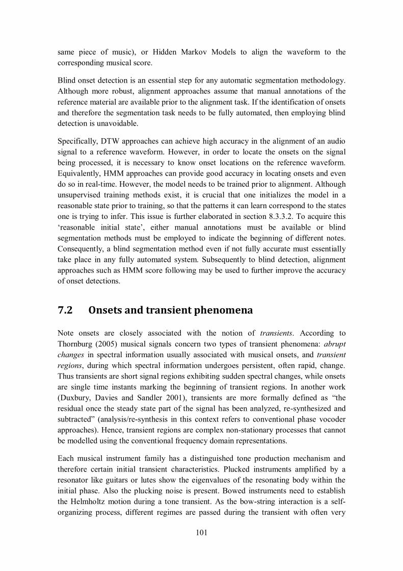
101
same piece of music), or Hidden Markov Models to align the waveform to the
corresponding musical score.
Blind onset detection is an essential step for any automatic segmentation methodology.
Although more robust, alignment approaches assume that manual annotations of the
reference material are available prior to the alignment task. If the identification of onsets
and therefore the segmentation task needs to be fully automated, then employing blind
detection is unavoidable.
Specifically, DTW approaches can achieve high accuracy in the alignment of an audio
signal to a reference waveform. However, in order to locate the onsets on the signal
being processed, it is necessary to know onset locations on the reference waveform.
Equivalently, HMM approaches can provide good accuracy in locating onsets and even
do so in real-time. However, the model needs to be trained prior to alignment. Although
unsupervised training methods exist, it is crucial that one initializes the model in a
reasonable state prior to training, so that the patterns it can learn correspond to the states
one is trying to infer. This issue is further elaborated in section 8.3.3.2. To acquire this
‘reasonable initial state’, either manual annotations must be available or blind
segmentation methods must be employed to indicate the beginning of different notes.
Consequently, a blind segmentation method even if not fully accurate must essentially
take place in any fully automated system. Subsequently to blind detection, alignment
approaches such as HMM score following may be used to further improve the accuracy
of onset detections.
7.2 Onsets and transient phenomena
Note onsets are closely associated with the notion of transients. According to
Thornburg (2005) musical signals concern two types of transient phenomena: abrupt
changes in spectral information usually associated with musical onsets, and transient
regions, during which spectral information undergoes persistent, often rapid, change.
Thus transients are short signal regions exhibiting sudden spectral changes, while onsets
are single time instants marking the beginning of transient regions. In another work
(Duxbury, Davies and Sandler 2001), transients are more formally defined as “the
residual once the steady state part of the signal has been analyzed, re-synthesized and
subtracted” (analysis/re-synthesis in this context refers to conventional phase vocoder
approaches). Hence, transient regions are complex non-stationary processes that cannot
be modelled using the conventional frequency domain representations.
Each musical instrument family has a distinguished tone production mechanism and
therefore certain initial transient characteristics. Plucked instruments amplified by a
resonator like guitars or lutes show the eigenvalues of the resonating body within the
initial phase. Also the plucking noise is present. Bowed instruments need to establish
the Helmholtz motion during a tone transient. As the bow-string interaction is a self-
organizing process, different regimes are passed during the transient with often very
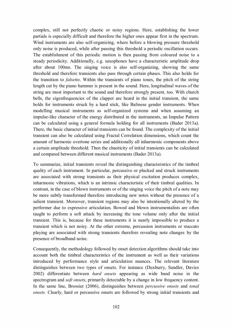
102
complex, still not perfectly chaotic or noisy regions. Here, establishing the lower
partials is especially difficult and therefore the higher ones appear first in the spectrum.
Wind instruments are also self-organizing, where before a blowing pressure threshold
only noise is produced, while after passing this threshold a periodic oscillation occurs.
The establishment of this periodic motion is then passing from coloured noise to a
steady periodicity. Additionally, e.g. saxophones have a characteristic amplitude drop
after about 100ms. The singing voice is also self-organizing, showing the same
threshold and therefore transients also pass through certain phases. This also holds for
the transition to falsetto. Within the transients of piano tones, the pitch of the string
length cut by the piano hammer is present in the sound. Here, longitudinal waves of the
string are most important to the sound and therefore strongly present, too. With church
bells, the eigenfrequencies of the clapper are heard in the initial transient, the same
holds for instruments struck by a hard stick, like Balinese gender instruments. When
modelling musical instruments as self-organized systems and when assuming an
impulse-like character of the energy distributed in the instruments, an Impulse Pattern
can be calculated using a general formula holding for all instruments (Bader 2013a).
There, the basic character of initial transients can be found. The complexity of the initial
transient can also be calculated using Fractal Correlation dimensions, which count the
amount of harmonic overtone series and additionally all inharmonic components above
a certain amplitude threshold. Then the chaoticity of initial transients can be calculated
and compared between different musical instruments (Bader 2013a).
To summarize, initial transients reveal the distinguishing characteristics of the timbral
quality of each instrument. In particular, percussive or plucked and struck instruments
are associated with strong transients as their physical excitation produces complex,
inharmonic vibrations, which is an intrinsic characteristic of their timbral qualities. In
contrast, in the case of blown instruments or of the singing voice the pitch of a note may
be more subtly transformed therefore introducing new notes without the presence of a
salient transient. Moreover, transient regions may also be intentionally altered by the
performer due to expressive articulation. Bowed and blown instrumentalists are often
taught to perform a soft attack by increasing the tone volume only after the initial
transient. This is, because for these instruments it is nearly impossible to produce a
transient which is not noisy. At the other extreme, percussion instruments or staccato
playing are associated with strong transients therefore revealing note changes by the
presence of broadband noise.
Consequently, the methodology followed by onset detection algorithms should take into
account both the timbral characteristics of the instrument as well as their variations
introduced by performance style and articulation nuances. The relevant literature
distinguishes between two types of onsets. For instance (Duxburry, Sandler, Davies
2002) differentiate between hard onsets appearing as wide band noise in the
spectrogram and soft onsets, primarily detectable by a change in low frequency content.
In the same line, Brossier (2006), distinguishes between percussive onsets and tonal
onsets. Clearly, hard or percussive onsets are followed by strong initial transients and
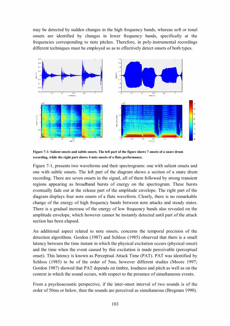
103
may be detected by sudden changes in the high frequency bands, whereas soft or tonal
onsets are identified by changes in lower frequency bands, specifically at the
frequencies corresponding to note pitches. Therefore, in poly-instrumental recordings
different techniques must be employed so as to effectively detect onsets of both types.
Figure 7-1: Salient onsets and subtle onsets. The left part of the figure shows 7 onsets of a snare drum
recording, while the right part shows 4 note onsets of a flute performance.
Figure 7-1, presents two waveforms and their spectrograms: one with salient onsets and
one with subtle onsets. The left part of the diagram shows a section of a snare drum
recording. There are seven onsets in the signal, all of them followed by strong transient
regions appearing as broadband bursts of energy on the spectrogram. These bursts
eventually fade out at the release part of the amplitude envelope. The right part of the
diagram displays four note onsets of a flute waveform. Clearly, there is no remarkable
change of the energy of high frequency bands between note attacks and steady states.
There is a gradual increase of the energy of low frequency bands also revealed on the
amplitude envelope, which however cannot be instantly detected until part of the attack
section has been elapsed.
An additional aspect related to note onsets, concerns the temporal precision of the
detection algorithms. Gordon (1987) and Schloss (1985) observed that there is a small
latency between the time instant in which the physical excitation occurs (physical onset)
and the time when the event caused by this excitation is made perceivable (perceptual
onset). This latency is known as Perceptual Attack Time (PAT). PAT was identified by
Schloss (1985) to be of the order of 5ms, however different studies (Moore 1997;
Gordon 1987) showed that PAT depends on timbre, loudness and pitch as well as on the
context in which the sound occurs, with respect to the presence of simultaneous events.
From a psychoacoustic perspective, if the inter-onset interval of two sounds is of the
order of 50ms or below, then the sounds are perceived as simultaneous (Bregman 1990).
104
Consequently, more recent studies (Klapuri 1999; Duxbury, Sandler and Davies 2002a;
as well as the MIREX evaluation measures) consider an onset as accurately detected, if
it falls within a 50ms time window around the actual physical onset. However, it is
clearly stated by MIREX that as onset detection is a pre-processing step, the real cost of
an error depends on the application following the task of onset detection13
.
Figure 7-2: The physical onset occurs at 2ms, but the new note will not be audible until about 40ms.
As was also discussed in section 2.4, 50 ms corresponds to a frequency of 20 Hz, which
is the lowest threshold of pitch perception. Also in vision, 50 ms is a basic integration
time, all events occurring within this 50 ms are integrated to one sensation. Therefore a
video stream needs to have a frame rate of at least 18 fps to appear as continuous.
Figure 7-2 presents an onset of a flute note, in which the physical excitation occurs at
2ms. The attack is not audible until about 50ms. Nevertheless, it is important to
highlight that for the purposes of the target application on NMP, the onset must be
detected as early as possible so as to allow concatenation to take place before the actual
note is made audible.
7.3 Typical blind onset detection methodology
Blind onset detection algorithms operate in three steps, which are: pre-processing,
reduction and peak-picking (Bello et al. 2005). Pre-processing is an optional step,
mostly appropriate to offline onset detection of music recordings. The reduction step
concerns the computation of an Onset Detection Function (ODF) as the value of one or
more temporal or spectral features computed over successive audio blocks of predefined
13 http://www.music-ir.org/mirex/wiki/2011:Audio_Onset_Detection
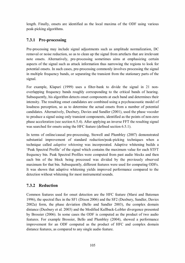
105
length. Finally, onsets are identified as the local maxima of the ODF using various
peak-picking algorithms.
7.3.1 Pre-processing
Pre-processing may include signal adjustments such as amplitude normalization, DC
removal or noise reduction, so as to clean up the signal from artefacts that are irrelevant
note onsets. Alternatively, pre-processing sometimes aims at emphasizing certain
aspects of the signal such as attack information thus narrowing the regions to look for
potential onsets. In such cases, pre-processing commonly involves processing the signal
in multiple frequency bands, or separating the transient from the stationary parts of the
signal.
For example, Klapuri (1999) uses a filter-bank to divide the signal in 21 non-
overlapping frequency bands roughly corresponding to the critical bands of hearing.
Subsequently, his algorithm detects onset components at each band and determines their
intensity. The resulting onset candidates are combined using a psychoacoustic model of
loudness perception, so as to determine the actual onsets from a number of potential
candidates. Alternatively, Duxbury, Davies and Sandler (2001), used the phase vocoder
to produce a signal using only transient components, identified as the points of non-zero
phase acceleration (see section 6.5.4). After applying an inverse FFT the resulting signal
was searched for onsets using the HFC feature (defined section 6.5.1).
In terms of online/causal pre-processing, Stowell and Plumbley (2007) demonstrated
substantial improvement of standard reduction/peak-picking techniques when a
technique called adaptive whitening was incorporated. Adaptive whitening builds a
‘Peak Spectral Profile’ of the signal which contains the maximum value for each STFT
frequency bin. Peak Spectral Profiles were computed from past audio blocks and then
each bin of the block being processed was divided by the previously observed
maximum for that bin. Subsequently, different features were used for computing ODFs.
It was shown that adaptive whitening yields improved performance compared to the
detection without whitening for most instrumental sounds.
7.3.2 Reduction
Common features used for onset detection are the HFC feature (Marsi and Bateman
1996), the spectral flux in the SF1 (Dixon 2006) and the SF2 (Duxbury, Sandler, Davies
2002a) form, the phase deviation (Bello and Sandler 2003), the complex domain
distance (Duxbury et al. 2003) and the Modified Kullback-Leibler divergence presented
by Brossier (2006). In some cases the ODF is computed as the product of two audio
features. For example Brossier, Bello and Plumbley (2004), showed a performance
improvement for an ODF computed as the product of HFC and complex domain
distance features, as compared to any single audio feature.
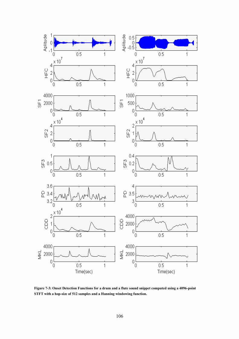
106
Figure 7-3: Onset Detection Functions for a drum and a flute sound snippet computed using a 4096-point
STFT with a hop-size of 512 samples and a Hanning windowing function.
107
Figure 7-4: Onset Detection Functions for a drum and a flute sound snippet computed using 2048 samples with
a hop size of 512 samples, zero padded to form a 4096 point window. No windowing function is used for this
transform.
108
Plenty of experimentation was conducted prior to designing the onset detection
algorithm to be used in the current system. A formal evaluation of the performance of
each feature for the task of onset detection is beyond the scope of this dissertation, as it
has been previously reported in several related publications (Brossier 2006; Brossier,
Bello and Plumbley 2004; Bello et al. 2005). However, for reasons of consistency and
in order to provide reasoning for the approach adopted in the present system, the
remaining part of this section demonstrates the performance of each feature for the
example drum and flute sound snippet of Figure 7-1.Specifically, the performance of
these features is demonstrated using two parameterisations of the STFT (see section
6.3): a) the commonly used STFT of 4096 samples having a hop size of 512 samples
and multiplied by a Hanning window and b) the parameterisation that was proposed for
early detections which uses 2048 samples zero padded to 4096 and a hop size of 512
samples, without multiplying by any windowing function (equivalent to using a
rectangular window). Figure 7-3 illustrates the ODFs computed using the
parameterisation (a), while Figure 7-4 illustrates the ODFs computed with the proposed
parameterisation (b). Although it is not obvious from the following figures it was
experimentally verified that using parameterisation (b) yields earlier detections, i.e.
closer to the physical onsets.
By observing these figures the following conclusions may be drawn: Firstly, it is a lot
easier to detect onsets on the drum sound, associated with percussive onsets having
salient initial transients. For this sound all features have a maximum value at the
location of onsets which is clearly not the case for the flute sound. For the flute sound
the most appropriate features are those based on Spectral Flux (i.e. SF1, SF2, and SF3).
Out of these three features, the SF3 feature seems to more successfully account for
onsets of both sounds, as it is independent of amplitude variations (see also section
6.5.3).
Finally, with respect to the parameterisation of the Fourier transform, it can be seen that
when using parameterisation (b), feature values are more ‘noisy’ than in
parameterisation (a). This noisy behaviour is caused by spectral leakage owing to the
use of a rectangular window, which does not fade out end-point discontinuities. In the
percussive drum sound, the noisy behaviour is less apparent because of dominating
noisy components of the signal itself. However, in both parameterisations the dominant
peaks of feature values owing to note onsets are clearly distinguishable. As was
discussed in section 6.3, parameterization (b) is preferred because, due to using fewer
audio samples (i.e. 2048 instead of 4096) on the analysis window, each captured block
(of 512 samples) has a higher contribution to the computed spectral features and more
importantly because, due to the rectangular window, it allows early detections, namely
before the onset appears in the center of the analysis window.
109
7.3.3 Peak-picking
Subsequently to reduction, temporal peak-peaking is applied in order to identify onsets
as the local maxima of the computed ODF.
Before computing the local maxima, post processing the ODF may be optionally
performed. In such cases, post-processing involves normalisation and DC removal so
that the ODF varies within the interval [0, 1] and possibly some smoothing in order to
remove unwanted noise. Obviously, normalisation and DC removal is applied only in
offline settings, while smoothing may be effectively and causally implemented in online
settings using for example a Finite Impulse Response (FIR) filter (Brossier 2006; Bello
et al. 2005).
Peak-picking aims at computing a threshold value, so that values of the ODF exceeding
that threshold are identified as onsets. The threshold may be either fixed (i.e. a constant
value over the entire duration of the signal) or it may be dynamically computed based
on previous ODF values, so as to account for variations owing to performance
dynamics.
Bello et al. (2005), used normalisation, DC removal and low-pass filtering for post-
processing various ODFs and then used a median filter to compute a dynamic threshold.
This median filter can be formulated as:
where D(n) is the ODF value of audio block n, δ and λ are positive constants and M
corresponds to the longest time interval on which the dynamics of the signal are not
expected to evolve, typically around 100ms. The computation of this threshold is non-
causal and therefore not applicable to online settings.
In causal settings, considering the mean value, in addition to the median, for the
computation of the dynamic threshold was proposed as a way to compensate for the
lack of DC removal and normalization (Brossier 2006; Brossier, Bello and Plumbley
2004). The corresponding dynamic threshold was formulated as:
In the respective implementation, namely the open source Aubio library14
, Brossier uses
α = 5 and b=1, therefore computing the threshold using a window which starts five
blocks before the current block and one block after the current block. Unfortunately,
this threshold is non–causal, but using b=1 introduces a latency of a single block in the
detection of onsets.
14 http://aubio.org/
110
Subsequently to the computation of the dynamic threshold, two further constraints may
be applied to the values exceeding the threshold. Specifically, in order to minimize false
detections Brossier (2006) proposed the use of a silence gate so as to reject spurious
detections in low energy areas, as well as rejection of an onset when it is detected very
close to another onset, based on a so called minimum Inter-Onset-Interval (IOI)
criterion.
7.4 Offline segmentation in the proposed system
For the application being investigated, robust onset detection is essential for producing
the audio segments that will be concatenated during live performance in order to
remotely re-synthesize the performance of each musician in real-time. For this purpose
and since the target usage scenario permits it, the respective algorithm exploits
information derived from the music score in order to increase the robustness of the blind
detection methodology. Hence, the resulting onset detection algorithm cannot be
considered ‘blind’ per se. However, it does not perform any score alignment either. The
score information exploited concerns the total number of notes the appearing in the
signal (i.e. the number of onsets that need to be found). This possibility simplifies the
peak-picking step of the blind detection methodology. As was discussed in section 0
peak-picking involves configuring a number of parameters (α, δ, λ) which need careful
consideration to successfully depict ODF thresholds for different instrumental timbres
and performance articulations. Consequently, the adopted approach can be regarded as a
hybrid onset detection scheme, which is based on the blind detection methodology,
however exploiting score information so as to provide increased robustness and allow
for a broad variety of instrumental sounds to be accurately segmented using the same
algorithm and the same parameterisation.
As shown on Figure 5-1, audio segmentation takes place offline and prior to NMP with
the objective of generating a pool of audio segments for each performer together with
their associated descriptors. The following subsection describes the onset detection
algorithm used for detecting segment boundaries and the one that follows describes the
process of computing segment descriptions.
7.4.1 A Robust onset detection algorithm
The ‘blind’ part of the algorithm uses the SF3 feature computed with an STFT of 2048-
samples zero-padded to form a 4096-point analysis window, which is not multiplied by
any windowing function (i.e. uses a rectangular window). The hop size is deliberately
small in order to provide increased time resolution in the detection of onsets, while zero
padding is used instead of highly overlapping signal windows to accentuate early
detections. As elaborated in section 7.3.2 and illustrated in Figure 7-4, this feature was
proven more effective in depicting onsets as local maxima of the corresponding ODF, in
comparison to alternative audio features. In the case of subtle pitch onsets as in the
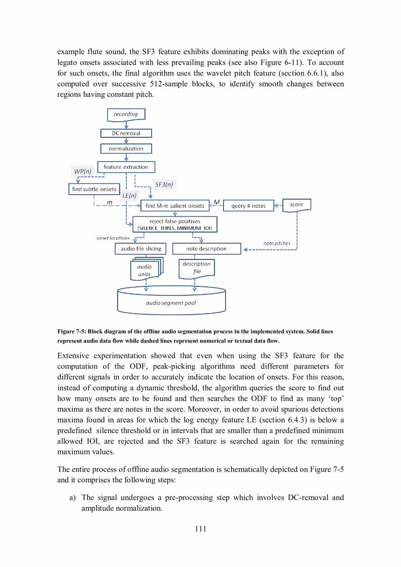
111
example flute sound, the SF3 feature exhibits dominating peaks with the exception of
legato onsets associated with less prevailing peaks (see also Figure 6-11). To account
for such onsets, the final algorithm uses the wavelet pitch feature (section 6.6.1), also
computed over successive 512-sample blocks, to identify smooth changes between
regions having constant pitch.
Figure 7-5: Block diagram of the offline audio segmentation process in the implemented system. Solid lines
represent audio data flow while dashed lines represent numerical or textual data flow.
Extensive experimentation showed that even when using the SF3 feature for the
computation of the ODF, peak-picking algorithms need different parameters for
different signals in order to accurately indicate the location of onsets. For this reason,
instead of computing a dynamic threshold, the algorithm queries the score to find out
how many onsets are to be found and then searches the ODF to find as many ‘top’
maxima as there are notes in the score. Moreover, in order to avoid spurious detections
maxima found in areas for which the log energy feature LE (section 6.4.3) is below a
predefined silence threshold or in intervals that are smaller than a predefined minimum
allowed IOI, are rejected and the SF3 feature is searched again for the remaining
maximum values.
The entire process of offline audio segmentation is schematically depicted on Figure 7-5
and it comprises the following steps:
a) The signal undergoes a pre-processing step which involves DC-removal and
amplitude normalization.
112
b) Feature extraction is applied in order to derive three features which are: the
instant wavelet pitch (WP), the normalized version of spectral flux (SF3), and
the log-energy (LE)
c) Subtle pitch changes are detected by examining the instant pitch WP. In specific,
a non-percussive onset is located at pitch changes for which the old pitch is
maintained for at least 100ms before the potential onset and the new pitch for at
least 100ms after the onset.
d) The score is parsed to determine the number of notes that must be detected, for
example M-notes.
e) If m-notes are detected as subtle pitch onsets, then the SF3 feature is searched
for the top M-m maximum values
f) For each such maximum value, the algorithm examines satisfaction of two
constraints: a) that the detected maximum is at least 50ms (defined by a global
constant named MINIMUM_IOI) apart from any previously detected onset and
that b) for the next 50ms (i.e. ATTACK_DURATION) there is at least one audio
block having a Log Energy (LE) value that exceeds -40dB (i.e.
SILENCE_THRESHOLD). If the detected maximum satisfies these constrained
it is recorded in the list of detected onsets, otherwise it is recorded in a list of
discarded candidates.
g) When the list of detected onsets reaches the desired length M, it is ordered in
time, so that earlier onsets appear in the list before later onsets.
h) For every onset in the ordered list, a new segment is stored in the pool of audio
segments and a line is added in the corresponding description file.
7.4.2 Generating Segment Descriptions
While segmenting each solo recording, the system generates a text file that describes the
duration, the RMS amplitude and the pitch of the note contained in each audio segment.
As described in section 9.3, these descriptions are used for computing expressive
deviations of the note performed during live NMP, compared to the corresponding note
segment maintained in the segment pool. The estimated deviations are subsequently
used to transform the retrieved segment in terms of loudness and duration, so as to more
closely match expressive utterances employed during live collaborative performance.
A precise description of the contents of the description file as well as an excerpt of an
example file is provided in section 10.3.2.3.
113
8 HMM Score Following
This chapter describes the methodology that was adopted for tracking the performance
of each musician during distributed live performance. Performance tracking was
achieved by means of score following based on Hidden Markov Models. Initially, the
chapter discusses the general conceptual approach and the applications targeted by
HMMs. The section that follows formulates their mathematical definition and the
adopted computational approach. As there are several alternative representations of
HMMs in tackling specific problems, the section that follows elaborates on several
design considerations that were confronted while experimenting with the system under
investigation. Finally, the last section of this chapter presents the model that was
implemented in the present system, as well as the methodology that was adopted for
efficiently training that model and using it in order to allow detecting note onsets in
real-time.
8.1 The HMM approach
A Hidden Markov Model (HMM) is a statistical model for determining the current state
of a system, which is assumed to be governed by a Markov process. A Markov process
is a stochastic process satisfying the Markov property, which requires that the process is
memoriless, meaning that future states depend exclusively on the present state and not
on preceding states. More concisely stated, HMMs assume that the current state is only
conditioned on the previous state.
In particular, HMMs attempt to extrapolate versatile information within data series.
Such versatile information is represented in system states. System states are not directly
observable and they are considered as hidden or latent variables of the model. However,
what is observable is a series of system measurements, termed as observations or
emissions, which are assumed to be highly correlated with the hidden states. To sum up,
an HMM determines the current state of a system, given its previous state and the
current system observations. Clearly, the design of an HMM for a specific task needs
careful consideration with respect to selecting appropriate system states and system
observations, so that states effectively match the information that needs to be
extrapolated and that observations are sufficiently correlated to system states so that
different states are associated with highly uncorrelated system observations.
HMMs are extensively used in pattern recognition and time series prediction in a variety
of disciplines ranging from financial forecasting (Park et al. 2009) to biological
sequence analysis (Bi 2009). In the audio domain and specifically in speech research,
HMMs have been widely used for the task of speech recognition as well as for speech
114
synthesis. In speech recognition, observations are formed from audio feature vectors
and states correspond to phonemes, syllables, or words. Therefore, given a feature
vector as well as the previously decoded state, the HMM determines the current
phoneme, or syllable (Rabiner and Juang 1993). In speech synthesis HMMs are used to
determine parametric representations of speech signals induced from textual
compounds. Subsequently, the determined parameters are applied on a parametric
model such as an articulatory or formant model of speech which generates the speech
signal (see also section 4.2).
In music, HMMs have been widely used for the task of audio-to-score alignment
(section 3.2.2). By the time of this writing no evidence has been found that HMMs can
be used for direct audio-to-audio alignment (i.e. without assuming the presence of a
score). This is inherently related to the types of problems addressed by HMMs, which
are not to align two sequences of the same data rate (as for example in DTW), but to
find correspondences among two series of related data, one of which represents system
observations and the other represents higher level models of reduced data rate such as
notes or chords. Accordingly, the audio signal to be aligned needs a higher level
structural representation, which is effectively provided by its music score.
In these systems the audio file is sliced in a number of audio blocks. Feature extraction
is applied on each block so as to provide a number of feature values per block. These
feature values form a feature vector and each feature vector is an HMM observation
symbol. Given the sequence of observations (feature vectors) the goal of audio-to-score
alignment is to find the most probable sequence of notes. In HMM terminology notes
are represented as states, therefore the idea is to find the note sequence that yields the
maximum probability for a given sequence of feature vectors. There are three types of
probabilities related with HMMs: initial probabilities, transition probabilities and
observation probabilities. Initial probabilities determine the initial state of the sequence,
namely the state at time zero. Transition probabilities determine the possible transitions
among states, e.g. which note follows the current note. Finally, observation probabilities
associate observations symbols with system states, i.e. determine whether a symbol may
be emitted while the system is in a specific state.
Whether or not the HMM corresponds to perception is still a question under debate. In
terms of melody, the implementation-realization theory of Narmour (1990) also
assumes a transition probability imposed by melodic expectations between adjacent
musical intervals, similarly to HMMs. Also the Goldstein optimum processor of pitch
perception presents a statistical model in which, pitch estimations of complex tones are
successfully derived using Gaussian probabilities for the observed harmonic structure
and a maximum likelihood criterion (Goldstein 1973). As early as 1956, Mayer
remarked that musical style and also the mental processes involved in the perception of
music may be regarded as a complex system of probabilities. Such probabilities model
expectations and tendencies upon which musical meaning relies (Meyer 1956). A
115
statistical approach on how probabilities shape music perception is more
comprehensively investigated in the book of Temperley (2007).
8.2 Mathematical Foundation
There are numerous of mathematical resources on Hidden Markov Models. This section
does attempt to provide elaborate mathematical details on the realization of HMMs.
Instead, it provides the basic mathematical concepts that are necessary for describing
how HMMs were represented and integrated in the present work. The section firstly
provides the mathematical definition of HMMs, and then it summarises the
computational approach employed in alignment tasks. The notation as well as the
computational approach presented here is based on two widely known tutorials on
HMMs (Rabiner 1989; Bilmes 1998).
8.2.1 Definition of an HMM
Mathematically formulated, if O = {o1, o2,..., oT} is a sequence of observations drawn
from an observation vocabulary V = {v1, v2, ..., vM} and Q = {q1, q2, …, qT} is a
sequence of hidden states derived from a set of possible states S = {s1, s2, ...,sN}, in
other words if at each time t, where Tt 1 ,then Vot and Sqt , the HMM is
defined as the tuple ),,,,( BAMN , where:
N: is the number of possible states in the model
M: is the number of possible observations symbols
A = {aij }:is the state transition probability matrix, namely the matrix
that contains the probabilities of moving from state si to state sj, for each
pair of states: NjiforsqsqP itjtij ,1),|(a 1
B = { bik }: is the observation probability matrix, namely the matrix that
contains the probabilities of observation symbols ok emitted while the
system is in state si for each pair of symbol and state:
MkandNiforsqvopb itktik 11),|(
π = {πi }: is initial state distribution, defining the probabilities that at time
1t the system is at state i , for each such state:
NiforsqP i 1),( 1
8.2.2 Hypothesis and computational approach
From a statistical point of view, an HMM is a probabilistic model of the joint
probability of two distributions of random variables O and Q. This joint probability is
made tractable (i.e. efficiently evaluated), due to two conditional independence
assumptions:

116
1. The tth hidden state qt depends exclusively on the previous hidden state, qt-1 :
2. The tth
observation symbol depends exclusively on the tth hidden state:
Computationally, the theory of HMMs tackles three problems:
1. Compute the probability of an observation sequence given the model, P(O|λ).
2. Find the optimal state sequence that best explains a series of observations given
the model. That is find Q = {q1, q2, …, qT}, when O = {o1, o2,..., oT} and λ are
known.
3. Find the optimal parameters of model λ that best explains the observation
sequence. This problem translates to computing the model
which out of all possible models maximizes the
probability of a given sequence of observations.
The second problem is often referred as HMM decoding and the third as HMM training.
This is not necessarily the order followed in solving an HMM problem. Usually,
problem 3 and 1 are performed prior to HMM Decoding (problem 2). Each of these
problems is efficiently solved using: the forward or the backward procedure (problem
1), the Viterbi algorithm (problem 2), the Baum-Welch algorithm also called
Expectation-Maximization (EM) algorithm for HMMs, or forward-backward algorithm
(problem 3). Problem 3 is by far the most difficult to compute. The EM-algorithm has
proven to be a robust way to estimate model probabilities given an observation
sequence. The idea of EM is to view these probabilities as part of the given
observations, so as part of a time series. As these probabilities and distributions are only
a small amount of parameters compared to the number of observations, the EM
estimates them as if there were missing data points in a long time series. The elaborate
mathematical description of these algorithms can be found elsewhere and is beyond the
scope of this document; however some essential key concepts are presented in the next
section.
Considering the case of audio to score alignment as an example, the main goal is to find
the sequence of states (e.g. notes) that corresponds to the sequence of observations (i.e.
feature vectors) per audio block, so to say per 512 samples of a monophonic audio
signal. This target is depicted in the second problem, which however assumes that the
model is known prior to determining the hidden states. Therefore, before approaching
the second problem, one needs to consider the third problem in order to find the optimal
model for the given sequence of feature vectors. However, in order to solve the third
problem, an efficient method for evaluating the probability of observations given a
model, i.e. the first problem needs to be tackled. Hence, all three problems must be
essentially addressed for any alignment task.
117
8.3 Design considerations
In order to design a model for a specific task, it is necessary to determine a number of
HMM attributes from a broad range of different alternatives. In fact, all models used in
the relevant literature allow for numerous variations in the representation of HMMs.
This section outlines the design questions that were confronted during the
implementation of the prototype system being investigated and summarizes the
conclusions drawn from extensive experimentation with different HMM
representations.
8.3.1 States, transitions and HMM topologies
HMM states must essentially correspond to the information that needs to be found by
the HMM. In audio-to-score alignment approaches, states are directly derived from
score events. For example, in monophonic audio segmentation by alignment, which
aims at identifying the instants of note onsets, three states such as attack, sustain and
rest are used for the representation of each note of the score (Schwarz, Cont and Orio
2006; Raphael 1999). When dealing with polyphonic music (Raphael 2004; Cont 2010)
the score is represented as a single pitch, a chord (pitches occurring simultaneously) or
silence at every change of polyphony (i.e. at each note start and note end). Alternatively,
in the work of Bello and Pickens (2005) and later Cho and Bello (2009) as the HMM is
used for harmonic content recognition instead of score alignment, states correspond to
24 major and minor triads, i.e. a pair of triads for each of the 12 pitches of the chromatic
scale.
Determining how to represent states also determines the types of transitions permitted
between system states. The overall behaviour with regard to process movement between
states, in other words the number of states and their associated transitions, constitute an
HMM topology. Different HMM topologies are appropriate for different types of
applications.
Figure 8-1, illustrates some popular HMM topologies derived from the book of Gernot
Fink (2008). In such diagrams, non-zero transition probabilities are depicted with
directed arrows and the sum of all probabilities departing from any single state is
always 1. It can be seen that all states are associated with self-transitions or loops. In the
case of forward topologies (i.e. when transitions move in one direction), self-transition
probabilities effectively depict the time spent at each state. Consequently in audio to
score alignment approaches, transition probabilities are informed by the rhythmic
structure of the score (Raphael 1999).
The simplest HMM topology is the linear topology (i.e. the system can either stay on
the same state or proceed to the next one) and the most complex is the ergodic model
(i.e. any state can be reached from any other state). The Bakis topology allows for
skipping individual states, while the left-right model provides more flexibility by
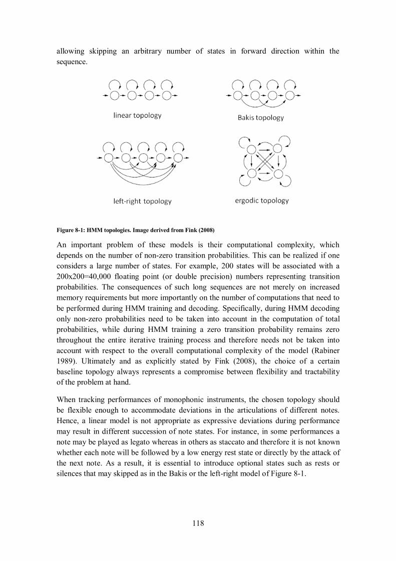
118
allowing skipping an arbitrary number of states in forward direction within the
sequence.
Figure 8-1: HMM topologies. Image derived from Fink (2008)
An important problem of these models is their computational complexity, which
depends on the number of non-zero transition probabilities. This can be realized if one
considers a large number of states. For example, 200 states will be associated with a
200x200=40,000 floating point (or double precision) numbers representing transition
probabilities. The consequences of such long sequences are not merely on increased
memory requirements but more importantly on the number of computations that need to
be performed during HMM training and decoding. Specifically, during HMM decoding
only non-zero probabilities need to be taken into account in the computation of total
probabilities, while during HMM training a zero transition probability remains zero
throughout the entire iterative training process and therefore needs not be taken into
account with respect to the overall computational complexity of the model (Rabiner
1989). Ultimately and as explicitly stated by Fink (2008), the choice of a certain
baseline topology always represents a compromise between flexibility and tractability
of the problem at hand.
When tracking performances of monophonic instruments, the chosen topology should
be flexible enough to accommodate deviations in the articulations of different notes.
Hence, a linear model is not appropriate as expressive deviations during performance
may result in different succession of note states. For instance, in some performances a
note may be played as legato whereas in others as staccato and therefore it is not known
whether each note will be followed by a low energy rest state or directly by the attack of
the next note. As a result, it is essential to introduce optional states such as rests or
silences that may skipped as in the Bakis or the left-right model of Figure 8-1.
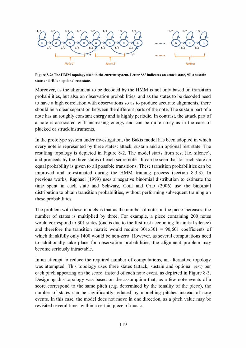
119
Figure 8-2: The HMM topology used in the current system. Letter ‘A’ indicates an attack state, ‘S’ a sustain
state and ‘R’ an optional rest state.
Moreover, as the alignment to be decoded by the HMM is not only based on transition
probabilities, but also on observation probabilities, and as the states to be decoded need
to have a high correlation with observations so as to produce accurate alignments, there
should be a clear separation between the different parts of the note. The sustain part of a
note has an roughly constant energy and is highly periodic. In contrast, the attack part of
a note is associated with increasing energy and can be quite noisy as in the case of
plucked or struck instruments.
In the prototype system under investigation, the Bakis model has been adopted in which
every note is represented by three states: attack, sustain and an optional rest state. The
resulting topology is depicted in Figure 8-2. The model starts from rest (i.e. silence),
and proceeds by the three states of each score note. It can be seen that for each state an
equal probability is given to all possible transitions. These transition probabilities can be
improved and re-estimated during the HMM training process (section 8.3.3). In
previous works, Raphael (1999) uses a negative binomial distribution to estimate the
time spent in each state and Schwarz, Cont and Orio (2006) use the binomial
distribution to obtain transition probabilities, without performing subsequent training on
these probabilities.
The problem with these models is that as the number of notes in the piece increases, the
number of states is multiplied by three. For example, a piece containing 200 notes
would correspond to 301 states (one is due to the first rest accounting for initial silence)
and therefore the transition matrix would require 301x301 = 90,601 coefficients of
which thankfully only 1400 would be non-zero. However, as several computations need
to additionally take place for observation probabilities, the alignment problem may
become seriously intractable.
In an attempt to reduce the required number of computations, an alternative topology
was attempted. This topology uses three states (attack, sustain and optional rest) per
each pitch appearing on the score, instead of each note event, as depicted in Figure 8-3.
Designing this topology was based on the assumption that, as a few note events of a
score correspond to the same pitch (e.g. determined by the tonality of the piece), the
number of states can be significantly reduced by modelling pitches instead of note
events. In this case, the model does not move in one direction, as a pitch value may be
revisited several times within a certain piece of music.
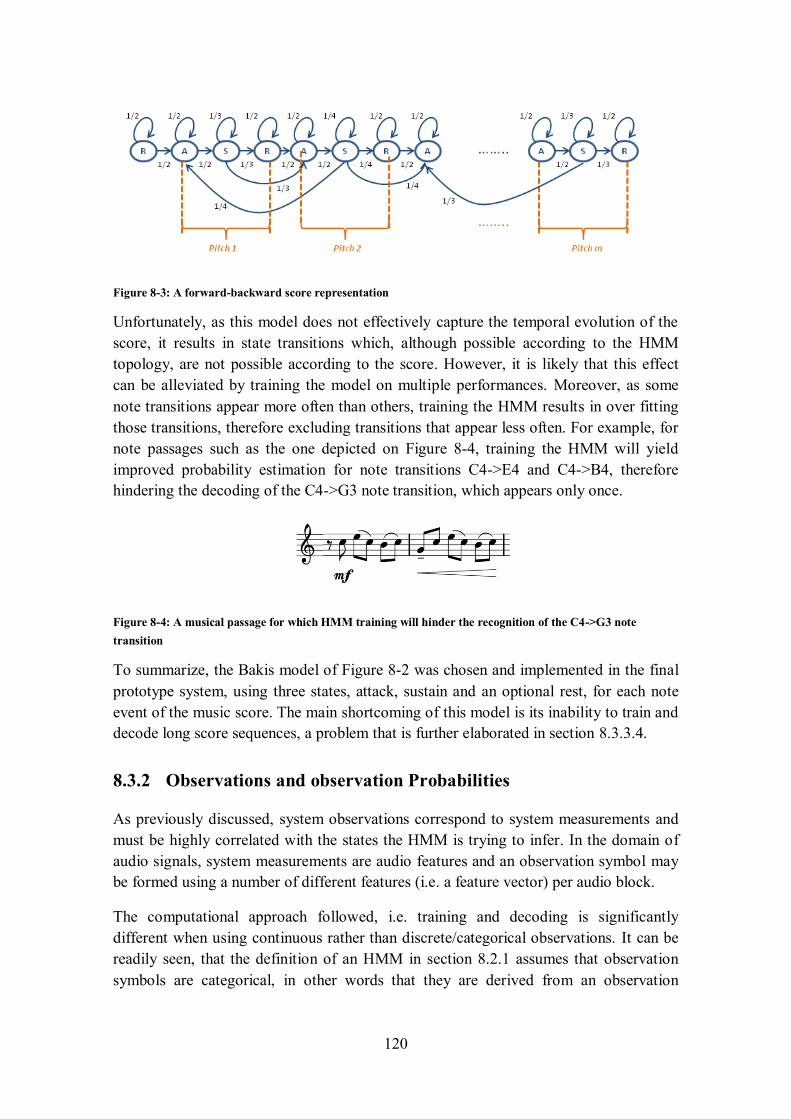
120
Figure 8-3: A forward-backward score representation
Unfortunately, as this model does not effectively capture the temporal evolution of the
score, it results in state transitions which, although possible according to the HMM
topology, are not possible according to the score. However, it is likely that this effect
can be alleviated by training the model on multiple performances. Moreover, as some
note transitions appear more often than others, training the HMM results in over fitting
those transitions, therefore excluding transitions that appear less often. For example, for
note passages such as the one depicted on Figure 8-4, training the HMM will yield
improved probability estimation for note transitions C4->E4 and C4->B4, therefore
hindering the decoding of the C4->G3 note transition, which appears only once.
Figure 8-4: A musical passage for which HMM training will hinder the recognition of the C4->G3 note
transition
To summarize, the Bakis model of Figure 8-2 was chosen and implemented in the final
prototype system, using three states, attack, sustain and an optional rest, for each note
event of the music score. The main shortcoming of this model is its inability to train and
decode long score sequences, a problem that is further elaborated in section 8.3.3.4.
8.3.2 Observations and observation Probabilities
As previously discussed, system observations correspond to system measurements and
must be highly correlated with the states the HMM is trying to infer. In the domain of
audio signals, system measurements are audio features and an observation symbol may
be formed using a number of different features (i.e. a feature vector) per audio block.
The computational approach followed, i.e. training and decoding is significantly
different when using continuous rather than discrete/categorical observations. It can be
readily seen, that the definition of an HMM in section 8.2.1 assumes that observation
symbols are categorical, in other words that they are derived from an observation
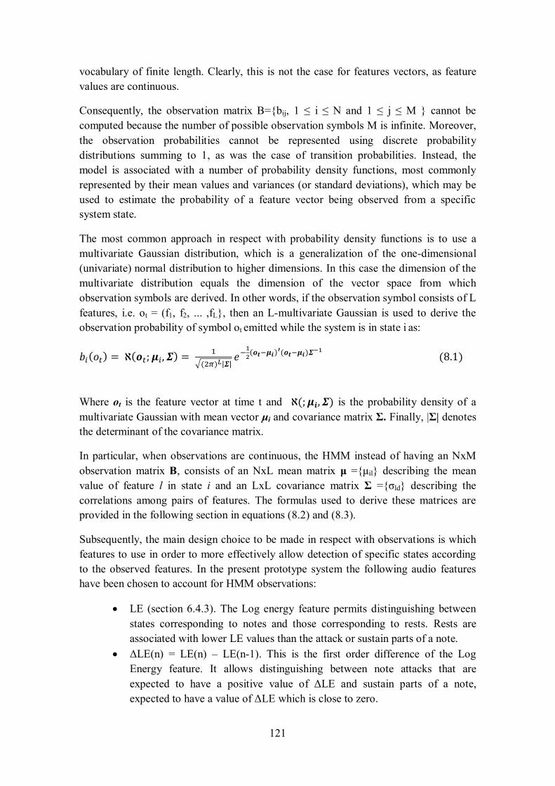
121
vocabulary of finite length. Clearly, this is not the case for features vectors, as feature
values are continuous.
Consequently, the observation matrix B={bij, 1 ≤ i ≤ N and 1 ≤ j ≤ M } cannot be
computed because the number of possible observation symbols M is infinite. Moreover,
the observation probabilities cannot be represented using discrete probability
distributions summing to 1, as was the case of transition probabilities. Instead, the
model is associated with a number of probability density functions, most commonly
represented by their mean values and variances (or standard deviations), which may be
used to estimate the probability of a feature vector being observed from a specific
system state.
The most common approach in respect with probability density functions is to use a
multivariate Gaussian distribution, which is a generalization of the one-dimensional
(univariate) normal distribution to higher dimensions. In this case the dimension of the
multivariate distribution equals the dimension of the vector space from which
observation symbols are derived. In other words, if the observation symbol consists of L
features, i.e. ot = (f1, f2, ... ,fL}, then an L-multivariate Gaussian is used to derive the
observation probability of symbol ot emitted while the system is in state i as:
Where ot is the feature vector at time t and is the probability density of a
multivariate Gaussian with mean vector μi and covariance matrix Σ. Finally, |Σ| denotes
the determinant of the covariance matrix.
In particular, when observations are continuous, the HMM instead of having an NxM
observation matrix B, consists of an NxL mean matrix μ ={μil} describing the mean
value of feature l in state i and an LxL covariance matrix Σ ={σld} describing the
correlations among pairs of features. The formulas used to derive these matrices are
provided in the following section in equations (8.2) and (8.3).
Subsequently, the main design choice to be made in respect with observations is which
features to use in order to more effectively allow detection of specific states according
to the observed features. In the present prototype system the following audio features
have been chosen to account for HMM observations:
LE (section 6.4.3). The Log energy feature permits distinguishing between
states corresponding to notes and those corresponding to rests. Rests are
associated with lower LE values than the attack or sustain parts of a note.
ΔLE(n) = LE(n) – LE(n-1). This is the first order difference of the Log
Energy feature. It allows distinguishing between note attacks that are
expected to have a positive value of ΔLE and sustain parts of a note,
expected to have a value of ΔLE which is close to zero.
122
SA (section 6.5.2): The spectral activity feature is primarily used as an onset
feature. In Figure 6-10, it can be seen that the distribution of this feature is
rather constant at all places except the location of onsets where local minima
are observed. Consequently, this feature can significantly improve the
probability of inferring a transition from a rest or sustain state to an attack
state (i.e. the onset)
SF3 (section 6.5.3). The same applies to the Spectral Flux feature which is
also used to increase the probability of an onset related transition.
ΔSF3: Experimentation showed that the first order difference of spectral flux
improves the quality of HMM alignment.
PSM (section 6.6.2) for each unique note present in the score. This feature
helps to distinguish among different pitches, and therefore among the states
corresponding to different notes.
ΔPSM for each unique note present in the score. As shown on Figure 6-17,
the distribution of this feature is constant throughout the signal apart from
the location of note onsets, where a sudden fluctuation is observed.
Therefore, in the current HMM implementation, the number of features L depends on
the number of unique notes appearing on the score. For example, if the score contains
50 notes of which 10 correspond to unique pitches then the dimension of the
observation symbol ot is L = 5+2x10 = 25 features and the number of states are N =
3x50+1= 151. The corresponding mean matrix will have a dimension of 151x25 and the
covariance matrix that of 25x25.
These features are computed for monophonic signals sampled at 44.1kHz and using a
16-bit sample resolution in audio blocks of 512 samples. For the computation of
spectral features, an STFT of 2048-sample windows zero-padded to 4096-points and a
hop size of 512 samples was used (section 6.3). Unfortunately, experimentation showed
that 256 sample blocks resulted in degradation of the alignment accuracy, as the
corresponding features do not contain enough information to sufficiently correlate with
HMM states. For example, if an attack state is expected to last while the logarithmic
energy is increasing and therefore the ΔLE feature is positive, then 256 samples may
not be enough to provide a positive value due to intermediate signal oscillations within
the 256-samples block.
8.3.3 Training Process
Training involves the estimation of HMM probabilities prior to HMM decoding. This
estimation concerns the initial probability matrix π, the transition probability matrix A,
and the emission probability matrix B. As we use continuous observations, instead of an
emission probability matrix we seek to estimate the mean vector matrix μ = {μil} and
the covariance matrix Σ = {σld}, where i is the state index and l, d are audio feature
indices. During decoding, the matrices μ and Σ are used to compute the probability bi(o-
t) of a feature vector ot being observed in state i using equation (8.1).

123
If for a given observation sequence O = {o1, o2, …, oT} the hidden state sequence Q =
{q1, q2, … qT } is known, then the mean vector μ and the covariance matrix Σ can be
easily computed for each state and for each feature as follows:
where fl(t) is the value of feature l at time t when the system is found in state si, and ni is
the number of audio blocks (out of the duration T of the entire sequence) spent in state
si.
The implementation of audio to score alignment in the current system uses a transition
probability matrix A which complies with the HMM topology shown on Figure 8-2.
Additionally, as the model follows a left-right direction and assuming the sequence
starts from the initial rest state, the initial probability matrix can be defined as π = {1.0,
0.0, ….,0.0}. This matrix corresponds to a system that starts from the initial (prior to
performing) rest and has zero probability in all other states at time t=1.
Consequently, if an accurate alignment is available prior to decoding it is possible to
estimate the model, including all probability matrices. However, in most cases no such
alignment exists, neither is easy to obtain. For this reason, several approaches (Raphael
1999; Cho and Bello 2005) employ unsupervised training methods in order to estimate
HMM probabilities. As already mentioned in section 8.2.2 the algorithm to efficiently
compute the HMM probabilities that best explain a sequence of observations is known
as Baum-Welch algorithm or Expectation Maximization for HMMs, or forward-
backward algorithm.
This algorithm is mathematically complex and involves the intermediate computation of
probabilities that are supplementary to π, A and B, known as forward and backward
probabilities. However, for reasons of consistency this section attempts to give a
simplistic and intuitive explanation of the entire process.
The idea is that the HMM model λ = (π, A, B) can be initialized by taking an initial
guess on the various probability values. Given this ‘guessed’ model, an alignment may
be computed using either the Viterbi algorithm used for decoding a sequence when the
model is known, or by computing the forward and the backward probabilities, which
provides an efficient procedure for computing the probability of a sequence P(O|λ) for
all possible state sequences. Then, given the resulting alignment Q, a new model λ’ =
(π’, A’, B’) can be estimated from λ as:
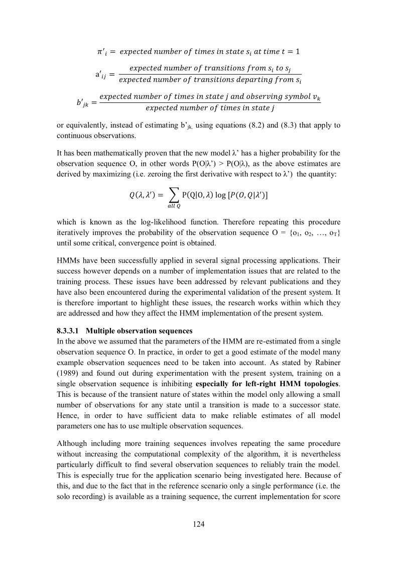
124
or equivalently, instead of estimating b’jk, using equations (8.2) and (8.3) that apply to
continuous observations.
It has been mathematically proven that the new model λ’ has a higher probability for the
observation sequence O, in other words P(Ο|λ’) > P(O|λ), as the above estimates are
derived by maximizing (i.e. zeroing the first derivative with respect to λ’) the quantity:
which is known as the log-likelihood function. Therefore repeating this procedure
iteratively improves the probability of the observation sequence O = {o1, o2, …, oT}
until some critical, convergence point is obtained.
HMMs have been successfully applied in several signal processing applications. Their
success however depends on a number of implementation issues that are related to the
training process. These issues have been addressed by relevant publications and they
have also been encountered during the experimental validation of the present system. It
is therefore important to highlight these issues, the research works within which they
are addressed and how they affect the HMM implementation of the present system.
8.3.3.1 Multiple observation sequences
In the above we assumed that the parameters of the HMM are re-estimated from a single
observation sequence O. In practice, in order to get a good estimate of the model many
example observation sequences need to be taken into account. As stated by Rabiner
(1989) and found out during experimentation with the present system, training on a
single observation sequence is inhibiting especially for left-right HMM topologies.
This is because of the transient nature of states within the model only allowing a small
number of observations for any state until a transition is made to a successor state.
Hence, in order to have sufficient data to make reliable estimates of all model
parameters one has to use multiple observation sequences.
Although including more training sequences involves repeating the same procedure
without increasing the computational complexity of the algorithm, it is nevertheless
particularly difficult to find several observation sequences to reliably train the model.
This is especially true for the application scenario being investigated here. Because of
this, and due to the fact that in the reference scenario only a single performance (i.e. the
solo recording) is available as a training sequence, the current implementation for score
125
follower does not train transition probabilities. The Baum-Welch algorithm is only used
to train observation probabilities. However, in a more elaborate scenario, recordings
obtained during offline rehearsals can be incorporated in training the model, therefore
providing a better estimate for all types of probabilities.
8.3.3.2 Obtaining an initial alignment
Previously, at the description of the training process it was mentioned that one should
start the iterative training process by taking an initial guess on model parameters (i.e.
initial, transition and observation probabilities). It is generally acknowledged that,
regardless the application domain, the initialization of model parameters is critical to the
performance of the model after training (Nathan, Senior and Subrahmonia 1996). In
fact, correct model initialization is essential when dealing with continuous system
observations (Rabiner 1989). Techniques such as clustering algorithms (e.g. segmental
k-mean clustering), Gaussian Mixture Models or the use of random values (Rabiner
1989; Rosa et al. 2007) have been proposed for different HMM tasks.
Correct model initialization largely depends on the task at hand. For example Bello and
Pickens (2005) used musical knowledge to inform the parameters of their HMM for
chord recognition, while previously Sheh and Ellis (2003) used random initializers for
the same task. For the task of audio to score alignment Cont (2004) used the Yin
algorithm (de Cheveigne 2002) for blind pitch detection to discriminate among different
pitch classes informing score states. Alternative approaches include generating a correct
alignment by synthesizing an audio waveform from the score, using a software program
or an API such as Timidity++15
(Hu, Dannenberg and Tzanetakis 2003), and optionally
aligning the synthesized waveform to an alternative recording using audio-to-audio
alignment techniques such as DTW or directly initialising the model based on the
synthesized waveform.
It is important to realize that this initial alignment should be as accurate as possible, so
that the patterns the HMM learns during training correspond to the states that need to be
inferred during HMM decoding. In the current HMM implementation, model
initialization is based on the offline audio segmentation algorithm that was used for
segmenting the solo recording (section 7.4.1). Based on the detected onsets, an
approximate alignment is inferred, which is further used for computing the mean vector
and covariance matrix from equations (8.2) and (8.3). The initial values of transition
probabilities are those depicted on Figure 8-2 and initial state probabilities are all zero
except from that of the first state which equals 1.0. Subsequently, the Baum-Welch
algorithm is applied on that initial model, so as to further refine observation
probabilities.
It is quite reasonable to wonder about what is the benefit of HMMs if a correct
alignment needs to be available prior to their decoding process. There are two benefits
in this respect: firstly that training on an accurate alignment/recognition will enable
15 http://timidity.sourceforge.net/
126
aligning/recognizing additional sequences bearing the same information content and
secondly that with HMMs it is possible to do so causally (i.e. online) and in real-time.
A further issue which is quite important to consider in the initialisation phase, is related
to the fact only transitions that are absolutely impossible should be assigned a zero
transition probability. It was previously mentioned (section 8.3.1) that zero-transition
probabilities remain zero throughout the entire iterative training process. This also holds
for observation probabilities (Rabiner 1989). Hence, in the present system, if the initial
alignment contains a skipped rest state, which is valid according to the topology of
Figure 8-2, then the computed observation probabilities of that state will be zero and
will remain zero after training. However, in an alternative performance, variations in
music interpretation may be such that the specific rest state is actually visited. In this
case the model will be unable to decode the performance further to the state having a
zero observation probability. To alleviate this problem in the implementation of the
final prototype, a common observation probability is computed for all rests, in other
words the mean values of features in rest states are computed based on all rests of the
initial alignment, regardless the preceding or following note and this also applies to the
computation of the covariance matrix. Therefore an equal observation probability is
obtained for all rest states using equations (8.2) and (8.3). Subsequently, Baum-Welch
training provides more accurate estimation of these probabilities resulting in different
values for different rest states. These trained values do not become zero so as to exclude
the possibility of expressive deviations in a different performance interpretation.
8.3.3.3 Numerical instability
As HMM training involves computing the product of a large number of probabilities
(i.e. forward and backward probabilities) that are numbers significantly smaller than
one, exceeding the machine’s numerical precision is a common problem during HMM
training.
The most common technique followed in order to avoid numerical underflow is to scale
these probabilities, by dividing them after each training iteration by their sum over all
states (Rabiner 1989). Alternatively, Mann (2006) proposes working with the
logarithms of probabilities. Unfortunately, as verified in the system under investigation,
working with logarithms in long sequences and left-right models increases the
computational complexity of the algorithm, and may therefore render the training
process entirely intractable.
8.3.3.4 Memory Requirements
One of the problems of Baum-Welch training is the inhibiting memory requirements
when attempting to model long audio sequences. These requirements stem from the fact
that for each audio block a number of multidimensional arrays holding forward and
backward probabilities per audio feature and per HMM state must be allocated.
Moreover, due to the numerical instability issued mentioned in the previous section,
these arrays must be of double precision (64 bit), otherwise it will be impossible to
perform computations on small probability values.
127
In order to realize the magnitude of this problem it is easy to find that one minute of
monophonic 44.1 kHz audio corresponds to (44100x60)/512 = 5,168 blocks of 512
samples. If we now consider the number of notes, for example 50 notes, of which ten
correspond to unique pitch values, we have 25 features and 151 states (see also section
8.3.2). One of the probability matrices ξt(i, j) used during training, records the
probability of being in state si at time t and in state sj at time t+1. Only this matrix
requires recording 5168x151x151 = 117,835,568 doubles that correspond to almost
943MB of computer memory, and this is only for one of the arrays!
Although this is a well known problem in biological sequence analysis (Miklós and
Meyer 2005) and several algorithms for reducing memory requirements have been
proposed (Khreich and Granger 2010), the problem has not been sufficiently addressed
for the task of audio–to-score alignment. A solution could be to split the observation
sequence into smaller and possibly overlapping segments and perform Baum-Welch
training for each of these segments. This has not been attempted in the implementation
of the system being investigated.
8.3.4 Decoding Process
HMM decoding involves finding the state sequence that best explains a given
observation sequence, when the model λ = (Ν, Μ, Α, Β, π) is known. This problem is
efficiently solved using the Viterbi algorithm, which is a dynamic programming
technique aiming at finding the optimal hidden state sequence by maximizing the
forward probability based on initial, transition and observation probabilities.
Mathematically stated, for a given λ and a given observation sequence O = {o1, o2, …,
oT}, the algorithm determines the single best state path Q = {q1, q2, … qT} by
maximizing P(Q|O, λ), which is equivalent to maximizing P(Q, O| λ). If the maximum
probability of the system reaching state si at time t is denoted as
then the optimal state sequence can be found by maximizing δt(i) at all times 1≤t≤T.
This probability can be computed by induction as:
It is reminded that aij is the transition probability from state i to state j and that bj(ot) is
the observation probability of symbol ot being emitted when the system is in state j.
If ψt(j) is an array that holds the state index i at time t-1 that optimizes the probability of
being at state j at time t, if in other words it holds the previous state for every current
state, then the complete Viterbi algorithm comprises four steps that can be formulated
as follows:
1) Initialization:
128
2) Recursion:
3) Termination:
4) Backtracking:
),
The backtracking step serves to adjust the preceding states once the terminating state
has been found, hence identifying the globally optimal state sequence. Clearly the
backtracking step is not causal, which renders the entire algorithm inappropriate for
real-time alignments. In respect with providing a causal equivalent Cho and Bello
(2009) proposed using an observation buffer of a small fixed length of the order of 5 to
15 blocks within which they performed backtracking, therefore decoding the state which
is 5 to 15 blocks past the current audio block. Alternatively, Orio and Dechelle (2001)
implemented their score scrolling algorithm by maximizing the probability of the state
sequence up to time t, known as forward probability:
which is computed recursively as:
Therefore, as a new block becomes available its state is determined from the previous
state by maximizing equation (8.5). As the forward probabilities αt(i) can become quite
large, it is necessary to scale, in other words normalize the probabilities among all
states j at each time step t, so as to avoid numerical overflow.
In the current system, two methods have been attempted for the implementation of real-
time decoding. The first attempts to maximize the value provided by equation (8.4) and
the second attempts to maximize the value of (8.5). Clearly both methods yield less
accurate alignments than the offline Viterbi algorithm due to probability maximization
on incomplete sequences. It should be noted that maximizing (8.4) or (8.5) is similar.
The major difference is the summation appearing in the formula (8.5) as opposed to
maximisation in formula (8.4). Experimental results showed maximizing (8.4) yields the
same alignment as maximizing (8.5).
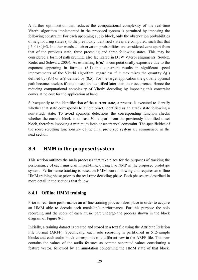
129
A further optimization that reduces the computational complexity of the real-time
Viterbi algorithm implemented in the proposed system is permitted by imposing the
following constraint: For each upcoming audio block, only the observation probabilities
of neighbouring states sj to the previously identified state si are computed, such that that
j-3 ≤ i ≤ j+3. In other words all observation probabilities are considered zero apart from
that of the previous state, three preceding and three following states. This may be
considered a form of path pruning, also facilitated in DTW Viterbi alignments (Soulez,
Rodet and Schwarz 2003). As estimating bi(ot) is computationally expensive due to the
exponent appearing in formula (8.1) this constraint results in significant speed
improvements of the Viterbi algorithm, regardless if it maximizes the quantity δt(j)
defined by (8.4) or αt(j) defined by (8.5). For the target application the globally optimal
path becomes useless if note onsets are identified later than their occurrence. Hence the
reducing computational complexity of Viterbi decoding by imposing this constraint
comes at no cost for the application at hand.
Subsequently to the identification of the current state, a process is executed to identify
whether that state corresponds to a note onset, identified as an attack state following a
non-attack state. To avoid spurious detections the corresponding function checks
whether the current block is at least 50ms apart from the previously identified onset
block, therefore imposing a minimum inter-onset-interval constraint. The specificities of
the score scrolling functionality of the final prototype system are summarised in the
next section.
8.4 HMM in the proposed system
This section outlines the main processes that take place for the purposes of tracking the
performance of each musician in real-time, during live NMP in the proposed prototype
system. Performance tracking is based on HMM score following and requires an offline
HMM training phase prior to the real-time decoding phase. Both phases are described in
more detail in the sections that follow.
8.4.1 Offline HMM training
Prior to real-time performance an offline training process takes place in order to acquire
an HMM able to decode each musician’s performance. For this purpose the solo
recording and the score of each music part undergo the process shown in the block
diagram of Figure 8-5.
Initially, a training dataset is created and stored in a text file using the Attribute Relation
File Format (ARFF). Specifically, each solo recording is partitioned in 512-sample
blocks and each audio block corresponds to a different row in the ARFF file. This row
contains the values of the audio features as comma separated values constituting a
feature vector, followed by an annotation concerning the HMM state of that block.
130
HMM states are textually represented as (MIDI pitch, state) pairs following the
topology depicted on Figure 8-2. In order to generate the feature vectors, feature
extraction is performed on the solo recording, while generating state annotations for the
initial alignment is achieved using the same algorithm for onset detection that was used
for the purposes of segmenting the solo recording and which was described in section
7.4.1.
Figure 8-5: Block diagram of the HMM training process. Solid lines represent audio data flows while dashed
lines represent numerical or textual data flow.
Annotations start with an initial rest state (0, Rest) until the audio block corresponding
to the first onset. The subsequent blocks up until 50ms (defined by a global constant
named ATTACK_DURATION) after the onset are marked as an attack state, for
example (60, Attack) for a MIDI pitch corresponding to middle C. The blocks that
follow are marked as sustain blocks (60, Sustain) up until the block where the Log
Energy feature falls below the threshold of -40dB (i.e. SILENCE_THRESHOLD). If
that or any previous sustain block corresponds to the next onset, the attack state of the
next onset is annotated, otherwise if after -40dB no onset has arrived, the blocks until
the next onset are marked as rest states as (60, Rest). Finally the annotated dataset is
stored in the ARFF file. A description of the use of ARFF files in the prototype system
as well as an extract of an example file is provided in section 10.3.2.1.
Following, the ARFF file is read and a model file describing the HMM is generated.
This file contains the names of the audio features that were used as well as the
131
probability values of all matrices: π, Α, μ, Σ. Initial probabilities are all zero apart from
the probability of the initial rest state, transition probabilities are those depicted on
Figure 8-2, while the mean vector and the covariance matrix are computed from
equations (8.2) and (8.3) using the annotated alignment provided by the ARFF file. A
description and an extract of an example model file are provided in section 10.3.2.2.
This initial model is denoted as λinit on the block diagram. The probability matrices of
that model as well as the feature vectors of the ARFF file are finally delivered to the
Baum-Welch algorithm. The Baum-Welch algorithm after running a number of
iterations which depends on the accuracy of λinit, converges to a new set of probability
matrices μ, Σ for the observation probabilities. This trained model λtrained is finally
stored in an additional model file.
With respect to the implementation of the training process, it is important to recapitulate
on two key points. Firstly, transition probabilities are not trained but instead retain the
values of Figure 8-2 so as to alleviate from problems caused by the fact that training is
performed on a single observation sequence (i.e. the solo recording), which is generally
inhibiting for training left-to-right HMM topologies, an issue that was elaborated in
section 8.3.3.1. Secondly, during the estimation of the initial model λinit, an equal
observation probability is computed out of all possible rest states, so as to avoid zero-
initialisation of the observation probabilities of certain rest states. As previously
discussed in section 8.3.3.2, these rest states may not be visited in one performance, but
visited in another performance. Initializing the corresponding probabilities to zero, may
lead to errors in the decoding process.
8.4.2 Real-time HMM Decoding
Figure 8-6 depicts the processes that take place during HMM decoding. These processes
are implemented on the transmitter of Figure 5-2.
The trained model file λtrained is loaded to memory prior to decoding, including feature
names and all HMM related matrices. Real-time audio capturing is based on callback
functions configured to use a buffer of 512 samples of monophonic 44.1kHz/16-bit
audio. As soon as a new block of audio becomes available, feature extraction takes
place to compute the features specified in the model file. Subsequently to the
computation of the feature vector, an observation probability bi(ot) is computed for each
score state from equation (8.1) using the values of μ, Σ provided by the model file. In
fact, as the computation of observation probabilities is based on exponents and the
number of score states may be quite high, in order to eliminate the number of
computations, bi(ot) is estimated only for neighbouring states of the one identified for
the previous audio block. As mentioned in section 8.3.4, this is a form of path pruning,
which is necessary to allow identifying HMM states before the next block of audio
becomes available.

132
Figure 8-6: Block diagram of the HMM decoding process. Solid lines represent audio data flows while dashed
lines represent numerical or textual data flow.
The computed observation probabilities as well as the transition probabilities are
fetched to the real-time Viterbi algorithm, which estimates the score state of the current
block. If that score state corresponds to an attack state following a non-attack state and
occurring after 50ms (i.e. greater than the MIMINUM_IOI global constant) from a
previously identified onset, then the current block is identified as an onset block and a
notification is sent over the network to indicate that the next audio segment must be
concatenated to the audio stream reproduced at the location of remote NMP
collaborators. This notification carries information about the RMS amplitude as well as
the duration of the previous note approximated by the corresponding Inter-Onset-
Interval (i.e. RMS (m-1), IOI(m-1)). As described in the next chapter, these two
attributes are used by remote receivers in order predict a gain factor and a time-scaling
factor that needs to be applied to the current segment, prior to signal concatenation.
133
9 Segmental Re-Synthesis
The title of this chapter has been deliberately chosen to distinguish the methodology
presented here from Concatenative Sound Synthesis (CSS) approaches. Conventionally,
and as was presented in chapter 4, CSS approaches imply the presence of an audio
corpus as well as a unit selection algorithm for selecting the units that best match the
specified target. As the problem addressed in the present work is a lot simpler in that
respect, using the term concatenative re-synthesis would be misleading given the
abundance of informative resources on CSS systems reported in the relevant research
literature.
The term segmental was found to more appropriately represent the methodology
employed in the present work and has been previously used in the speech coding
domain (see section 4.2). In the present context, the aim of the synthesis step is to
generate the performance of each musician at remote network locations using the audio
segments of his/her solo recording, which were accumulated using automatic offline
audio segmentation techniques. Clearly, the pre-segmented solo performance will be
very different from the live performance, not only because the latter is collaborative and
therefore follows the performance of other musicians, but also because music
interpretation is greatly influenced by the instantaneous mental and emotional state of
performers, and is therefore unique every time a piece is performed, even by the same
performer.
Thus, the present chapter initially discusses theoretical studies on expressive
performance, in an attempt to discern the type of interpretive deviations that may
introduced in different performances of the same piece of music. Then, the chapter
provides an overview of the processes undertaken during unit concatenation in relevant
concatenative music synthesis and computer accompaniment research initiatives. The
final section presents the approach adopted by the prototype system under investigation
and discusses the quality of the synthesized audio signals..
9.1 Rendering expressive musical performance
It is well known that faithful rendition of a musical score sounds machine-like and
musically uninteresting. In the western tradition, music scores have been a necessary
means of communicating composers’ intentions to potential performers. However, the
performer is offered plenty of freedom to interpret the music score using his/her own
understanding of musical meaning. Consequently, in the cases of non-improvisatory
music, musical expression may be attributed to deviations from a pre-transcribed
musical score. The prevalent deviations are related to inter- and intra-note attributes
134
such as timing duration and loudness (Ramírez et al. 2007), therefore accounting for
tempo deviations, dynamics, articulation (i.e. the type of transition among consecutive
notes) and less often deviations in pitch or intonation. However, depending on the
instrument, performers employ additional cues to manifest their intentions with respect
to expressive interpretation. For example, chord asynchronies (i.e. slight timing
deviations in the playback of different voices in polyphonic or harmonic context), the
use of piano pedal, or alternative deviations such as slight portamenti, tremolo or
vibratos present examples that define the unique character of a music performance.
Nevertheless, most of these intentions are subliminal and not readily tractable.
To provide an understanding on the expressive aspects introduced by deviating from a
score, music performance is often compared to speaking or reading from text (Delgado,
Fajardo and Solana 2011). If multiple people are asked to read the same text, the
produced sounds will be considerably different in terms of prosodic nuances rhythmic
stress or intonation. This analogy has been inspiring for several research initiatives. For
example in the work of Thompson, Schellenberg and Husain (2004), it was shown that
musically trained adults performed better than untrained in identifying emotions
conveyed by speech prosody. In another work, Coutinho and Dibben (2012) showed
that emotions in music and speech prosody can be predicted from seven
psychoacoustically relevant features: loudness, tempo/speech rate, melody/prosody
contour, spectral centroid, spectral flux, sharpness, and roughness.
Interestingly, expression of music emotion is predominantly, although not exclusively,
driven by performers’ intentions. For example, Widmer and Goebl (2004) defined
expressive music performance as “the deliberate shaping of the music by the performer
by means of continuous variations of timing loudness and articulation.” Skilled
professional performers apply such deliberate warping of expressive parameters so as to
develop their own signature-sound that distinguishes them from other performers. In
this line, a number of research efforts are being invested in developing machine learning
models that are able to recognize individual artists from their recordings (Saunders et al.
2008; Molina-Solana, Arcos and Gomez 2008). However, performances of the same
piece of music, even by the same performer may be very different from one another
depending on other factors, such as performer’s psychological mood (Gabrielson 1995;
Rigg 1964), fatigue or even the acoustics of the physical location in which music is
performed. Although sparsely investigated (e.g. Kalkandjiev 2013; Hatlevik 2012),
room acoustics may play an important role on how performers communicate music to
their surrounding environment.
Notably, a large number of studies on expressive performance approach music
expression from the structure residing within the music piece. Musicological studies
such as those of Sloboda (1983) observed that pianists tend to play louder and more
legato the notes at beginning of measures. Moreover, it was noticed that the beginning
and end of phrases are slower than the rest. With respect to harmonic progressions and

135
musical expression, Palmer (1996) showed that melodic expectation is influenced by the
energy used in playing the different notes.
Besides their musicological interest, studies in expressive music performance are often
conducted for the purposes of computational modelling to be ultimately applied in the
design of systems capable of rendering expressive performances. Evidently,
computational models of expressive music performance are already capable of
emulating human performances. In 2002, the Rencon, performance rendering contest
was created to offer subjective evaluations of systems generating expressive
performances. The contest employs a human judge to determine whether a performance
is artificial or human in accordance with the Turing test (Hiraga et al. 2004), as well as
to evaluate these systems in terms of their capability to demonstrate different factors
such as conveying emotional content or highlighting musical structure (Katayose et al.
2012).
Delgado, Fajardo and Mollina-Solana (2011) present a comprehensive review of
approaches in computational music performance and discern three research strategies:
(a) analysis-by-synthesis, (b) analysis-by-measurement and (c) performance systems
based on artificial intelligence. Analysis-by-synthesis is concerned with embedding
performance rules defined by the experience of an expert musician (Friberg Bresin and
Frydén 1998; Zanon and Poli 2003). Analysis-by-measurement systems derive
performance rules from acoustic analysis and statistical processing of recorded
performances (e.g. Todd 1992). In contrast to these approaches, the works of Widmer
(2003; Grachten and Widmer 2012) propose the use inductive machine learning applied
on large music corpora.
Expressive music performance is not the main focal point of this work. However,
synthesizing an audio stream from a pre-segmented performance requires careful
consideration of expressive aspects in order to retain the interpretive nuances of the live
recording in the synthesized audio stream. The sections that follow describe this process
from the perspective of audio signal processing.
9.2 Technical approaches to segmental re-synthesis
Re-synthesis of audio from pre-recorded segments is a task relevant both to CSS, as
well as computer accompaniment systems. In computer accompaniment, synthesis is
essentially performed in real-time while in CSS systems it may be performed either
offline or in real-time context, depending on the application scenario. As was seen in
section 4.4, most real-time CSS approaches aim at artistic exploration rather than high-
fidelity instrumental synthesis. Consequently in these initiatives, signal inconsistencies
due to poor concatenation quality are neither critical nor necessarily undesirable.
This section reviews alternative methodologies that are commonly adopted when
synthesizing a waveform using audio samples, so as to highlight differences among
136
methodologies and provide an understanding on the choices that were made in the
present work. When re-synthesizing a signal from audio segments, sample processing
needs to take place for two reasons: firstly to transform each segment in terms of
amplitude, duration and sometimes pitch, so as to better match the required target, and
secondly to eliminate perceivable artefacts that are caused by amplitude, pitch and
possibly timbre discontinuities at the junction point of two consecutive segments. In the
approach proposed here, it is important to elucidate that the occurrence of
discontinuities is caused by timing deviations in the occurrence of note onsets between
the pre-segmented solo performance and the live performance of each musician. These
timing deviations require time-scaling applied on note segments. Apart from time-
scaling amplitude transformations are also applied to account for deviations in
performance dynamics. Collectively, these two transformations are the reason of
consecutive segment discontinuities. If there were no transformations, then no
discontinuities would occur, but that would be equivalent to rendering the original audio
file without adapting it to the context of the live performance.
The next two subsections describe solutions to these two problems (i.e. transformation
and concatenation), while the section that follows describes the adaptation of this
problem to real-time settings. Representative examples from the relevant literature are
also provided.
9.2.1 Segment transformations
This stage is meant to transform the audio segment, most commonly in terms of
amplitude and duration and sometimes in terms of pitch as well, so as to better match
the desired target waveform. Amplitude transformations are pretty straightforward and
they conventionally involve multiplication of the entire segment by a gain or attenuation
factor. Regarding duration and pitch, the rudimentary approach involves re-sampling the
signal at a different rate than the one it was originally sampled. This technique is
inspired from the old days of analogue recording technology, where the ratio of
recording and playback rates alters the signal both in terms of duration as well as in
terms of pitch.
To perform duration and pitch modifications independently of each other, two
established techniques are commonly used: the phase vocoder which operates on the
spectral domain of the signal and the Pitch Synchronous Overlap Add (PSOLA)
transform, which operates on the time domain. Implementations of these two techniques
may greatly vary depending on the content of the signals being processed as well as on
potential requirements for low computational cost and real-time operation.
As will be seen in the next section, none of these methods has been precisely integrated
in the prototype system under investigation. The assumptions holding for the signals
being treated in this work (see section 5.3), largely simplify the problem of segment
transformations, for which a novel and intuitive approach has been adopted.
137
Consequently, no detailed mathematic or algorithmic description of phase vocoder and
PSOLA methods is provided in this chapter. However for reasons of consistency, a
qualitative and hopefully intuitive explanation of these techniques is provided in the
following subsections.
9.2.1.1 Phase Vocoder Transformations
The phase vocoder, originally introduced by Flanagan and Golden (1966), is a
technique for independently varying the pitch and the duration of an audio waveform
using the Short Term Fourier Transform (STFT), i.e. the Fourier Transform of
consecutive windowed and overlapped blocks of audio.
Phase vocoder time scaling is achieved by performing STFT analysis of the audio signal
and then applying the inverse transform by using a different amount of overlap than the
one used in the analysis step. Precisely, given a time scaling factor α, the analysis hop-
size Ra is varied with respect to the synthesis hop-size Rs, such that their ratio yields the
scaling factor, i.e. α = Rs/Ra. Conventionally, a 75% overlap at the output is considered
a good practice so as to avoid amplitude modulation due to phase inconsistencies.
Hence, Ra is varied in respect to Rs which remains constant at 75% of the STFT window
function.
Clearly, using a different amount of overlap between analysis and synthesis yields phase
discontinuities in the synthesized output, which can be corrected by applying the inverse
STFT using the analyzed spectral magnitudes and a phase which is estimated from the
phases of the original signal and adjusted by an amount that corresponds to the new hop
size. This is known as phase propagation and it ensures horizontal phase coherence,
namely phase consistency between successive audio blocks for each frequency
component. Unfortunately, this phase correction ruins the phase relationships between
different frequency components of the same audio block, known as vertical phase
coherence. In phase propagation, the same amount of phase correction is applied to all
frequency bins. However, as generally the signals being processed contain non-
stationary sinusoidal components, phases are not linearly related to the different
frequency bands. Absence of vertical phase coherence results in a degradation of
timbral quality, so that the resulting signal sounds more ‘smeary’ or ‘phasey’. For this
reason, an improved phase vocoder implementation (Laroche and Dolson 1999)
proposes a technique known as phase locking. Phase locking attempts to find the
sinusoidal components of the signal as the most dominant peaks of the spectrum of each
frame. Then it updates the phases of the non-sinusoidal components by preserving their
phase relationship to the closest sinusoidal component, after the last has been phase
corrected for horizontal phase coherence.
The most prominent application of the phase vocoder is on speech signals and the
synthesis of the singing voice (Laroch 2003; Bonada and Loscos 2003). This is
probably related to the spectral content of speech signals which are dominated by voice
formants corresponding to the acoustic resonances of the vocal tract. Formants appear
as dominating sinusoidal components; hence phase locking to these components
138
provides a more realistic phase approximation. In the case of music however, sinusoidal
components may be less apparent and even more so for percussive sounds as well as
during the initial transients. The duration of percussive sounds, such as drum sounds
cannot be controlled by the performer (no sustain state is present in the amplitude
envelope). Therefore, when for example stretching or shrinking a percussive sample in
time, one should simply increase or decrease the spacing among consecutive events
rather than performing a uniform stretch or shrink on the entire waveform. This is not
taken into account by phase vocoder time scaling and has to be treated in dedicated
implementations. When time scaling a percussive sound or a transient, even if perfectly
reconstructing its spectral content, its timbre will sound unnatural and therefore
perceptually distorted.
This problem has been addressed by (Duxbury, Davies and Sandler 2002b), where a
signal is firstly separated into its transient and steady state parts by means of multi-
resolution analysis, and then phase vocoder time scaling with phase locking is applied
to the steady (quasi-stationary) parts of the signal. This is clearly an offline, non-causal
process. However, in (Barry, Dorran and Coyle 2008) a real-time solution is provided
called transient hoping. In this work a measure of the ‘percussivity’ of the sound is
defined which looks at the rise of energy in dB between successive hops, summed for
all frequency bins. The audio frames for which this measure exceeds a predefined
threshold are characterized as transient and retained in the times-scaled signal without
any modification.
Phase vocoder pitch scaling on the other hand, is conventionally performed in two steps
which are re-sampling the signal to achieve the required pitch and then perform phase
vocoder time scaling to regain its original duration. For example to raise the pitch by a
factor of two one would half the sampling rate (i.e. skip every other sample of the
original waveform) and then time stretch the resulting signal by a factor of two (Laroche
2002). However, direct manipulation of the frequency partials of the signal has also
been proposed (Laroche and Dolson 1999). Direct frequency domain manipulations are
less favoured due to the fact that, firstly, they require a very high frequency resolution
and secondly that they are computationally more expensive due to the large number of
multiplications involved (Laroche 2002).
A real-time version of phase vocoder pitch shifting that does not require time scaling is
presented in (Barry, Dorran and Coyle 2008). In this paper, re-sampling at the required
rate is performed within a window that has a length which is multiplied by the pitch
scaling factor (i.e. βΝ where β is the pitch scaling factor and Ν the length of the FFT
window), therefore the duration is not affected. However, such re-sampling requires
phase correction by an amount affected by β and subsequent phase locking to
additionally maintain vertical phase coherence.
The phase vocoder is by far the most commonly used technique in CSS and computer
accompaniment systems. In CSS it has been used by Maestre et al. (2009) in offline
context for synthesizing expressive saxophone performances from contextually
139
informed note segments (see also section 4.3.2.1). In computer accompaniment systems,
the Music-Plus-One system developed by Raphael (section 3.2.4) uses the phase
vocoder to control the playback rate of the orchestral accompaniment of a live solo
performer. In this case the orchestral recording has been manually indexed and an
HMM of its alignment to the corresponding score is constructed offline. During live
performance a different HMM that corresponds to the soloist (trained during rehearsals)
is used to detect new onsets of the live solo. Subsequently, the duration of the orchestral
recording is appropriately scaled to synchronize with the solo performance at certain
points that represent short-term synchronization goals (Raphael 2003). This system does
not report on any mechanism for eliminating signal discontinuities. This is due to the
fact that no parts of the orchestral recording are skipped and therefore no discontinuities
are introduced, its only the playback rate that is continuously adjusted.
9.2.1.2 SOLA transformations
The SOLA (Synchronized OverLap Add) method was originally proposed by Roucos
and Wilgus (1985). It exists in many variations such as Waveform Similarity Overlap
Add (WSOLA) (Verhelst and Roelands 1993), Time Domain TD-PSOLA (Moulines
and Charpentier 1990), MultiBand Resynthesis Overlap Add (MBROLA) (Dutoit
1996), etc. The principle is essentially the same: Firstly, the pitch frequency of the
signal is detected by an f0 estimation algorithm. Following, the signal is windowed
commonly by using a Hanning window spanning two periods of the fundamental
frequency and centered on the maxima of signal energy. To increase or decrease the
pitch of the signal, consecutive windows are placed closer together or further apart
respectively. Finally, the overlapping parts of the signal are added to produce the final
waveform. In the case of time scaling, certain windows are duplicated to achieve
lengthening or skipped to achieve shortening. In both cases the resulting signal is
overlapped-added.
SOLA is commonly used in text-to-speech synthesis and has been impressively used in
synthesizing a choir in real-time from recordings of solo singers (Schnell et al. 2000). A
main problem of the algorithm arises when the sounds to be treated are not periodic, as
is the case of ‘unvoiced’ sounds. In such cases, a default window length of 10ms is used
while caution must be taken to avoid introducing artificial pitch correlations resulting in
a flanging-like effect. Common techniques in avoiding such correlations include phase
randomization (Richard and d’Alessandro 1996) at the non-periodic parts of the signal.
In the case of acoustic instruments, the same problem arises during note transients as
well as percussive sounds. In respect with preserving the distinctive timbre of note
transients and avoiding their repetitions, the same method as in phase vocoder is applied
by subtracting the transient components before PSOLA and then re-applying them after
synthesis (von dem nesebeck, Ziraksaz and Zölzer 2010).
Generally, most SOLA approaches are highly computationally efficient but their
performance relies on the periodicity of the signals being processed, as well as the
amount of required scaling. It is well known that scaling up or down by more than a

140
factor of two may result in considerable signal degradation. Modifications of the main
algorithms are occasionally proposed to allow high quality of transformations within a
wider scaling range (Cabral and Oliveira 2005; Bárdi 2006).
SOLA has been used in offline context in the Audio Analogies project (Simon et al.
2005). This project uses individual notes or pairs of notes to construct the waveform of
a music piece given its music score. Audio segments are re-sampled to achieve pitch
transformations, while their duration is scaled by means of SOLA.
Additionally as already mentioned, Schnell et al. (2000) used PSOLA in real-time
context to reproduce a choir sound from a single recording of a solo choir singer.
Analysis of the solo recording is performed offline and it comprises two phases:
separation between voiced (harmonic) and unvoiced parts and detection of marker
positions on the harmonic parts. These PSOLA markers indicate windowing positions
and they are placed pitch-synchronously (i.e. so that their distance corresponds to the
period of the fundamental frequency) and centered on the local maxima of signal
energy. Finally during synthesis, a marker file and the corresponding waveform are read
and a real-time algorithm applies replication of voices and PSOLA transformations so
as to obtain a distinctive character for each replicated voice. Unvoiced signal parts are
re-synthesized using some variation of granular synthesis.
9.2.2 Eliminating perceptual discontinuities
When concatenating transformed audio frames, phase and spectral shape discontinuities
occur. Such discontinuities are easy to handle in offline context but become more
difficult in real-time applications.
Solutions range from a simple amplitude cross-fade within a range of 10-100ms
(Schwarz et al. 2006; Dannenberg 2006) to more complex phase and spectral shape
interpolation spanning several frames in order to provide a smooth transition (Bonada
and Loscos 2003). In the work of Maestre et al. (2009) amplitude and pitch
discontinuities are smoothed using cubic spline curves so as to synthesize legato notes.
A simpler approach is presented by (Simon et al. 2005) where the optimal point of
intersecting the two segments is estimated by calculating their cross correlation. The
two segments are then intersected at the maximum of their cross correlation and
smoothed by a linear cross fade.
In real-time settings it is impossible to prepare the elimination of discontinuities
beforehand because the point of intersection is not known until the next segment needs
to be rendered. Therefore any time or spectral domain interpolations can only occur
within a single audio frame.

141
9.2.3 Real-time approaches and the need for anticipation
Several studies are being conducted with the aim of understanding the cognitive
processes that enable musicians to synchronise during ensemble performance (Rasch
1988; Keller 2007; Goebl and Palmer 2009). Studies of computational music
performance confirm tempo and dynamics as the most prominent resources available for
musicians to convey emotion and meaning in non-improvisatory music (Widmer and
Goebl 2004). As ensemble performance involves actions coordinated within small
fractions of seconds, collaborating musicians employ a great amount of cognitive
anticipation. Anticipating and therefore scheduling tempo and dynamic deviations both
at the macroscopic (i.e. for the overall piece) and the microscopic level (i.e. within small
groups of note events in a way that does not contribute to the macroscopic level) is
informed by three types of information sources: rehearsals, the score of the music work
and by continuously monitoring musical events during live performance (Marchini,
Papiotis and Maestre 2012).
Rehearsals help members of ensemble performance establish a common goal; a unified
concept of the ideal sound (Keller 2007). Performance goals are developed through
individual practice and collaborative rehearsals and aim at establishing a plan that
guides the motor processes involved in translating goal representations into appropriate
body movements (Gabrielson 1999).
Regarding the score, Raphael (2003) highlights that the music score should not be
viewed as a rigid grid prescribing the precise times at which musical events occur;
rather the score gives the basic elastic material which will be stretched in various ways
to produce the actual performance. The score simply does not address most interpretive
aspects of performance.
During live ensemble performance, Keller (2007) uses the term ‘adaptive timing’ to
refer to the process of adjusting musical performance according to the temporal
evolution of performance up to that time. Specifically, Keller assumes that the human
brain is capable of instantiating timekeepers that can be used to control the temporal
aspects of perception and action. These timekeepers are adjusted using error correction
processes that are initiated upon the occurrence of asynchronies in the timing of actions
undertaken by the various performers.
A more elaborate account on psychological and cognitive theories of timing
synchronisation is provided in Bader (2013b). It appears that traditional theories on
rhythm perception (Wing and Kristofferson 1973) show that when tapping on a
rhythmic pattern the timing deviation of each event depends on the deviation of the
previous event, so that an IOI arriving later (or earlier) than dictated by the rhythmic
pattern will be followed by an IOI arriving earlier (or later respectively) in a attempt to
correct the previous tap. This could be very well represented by a Markov chain as each
note event depends exclusively on the previous event. Yet, subsequent studies
investigating longer tapping series (e.g. Haken, elso and Bunz 1985; Delignières,

142
Lemoine and Torre 2004) showed that long–term memory is likely to further influence
the perception of rhythm. Notably, this is interpreted as the 1/f noise pattern of human
cognition (Gilden 2001). For example Pressing (1999) suggested using a moving
average to model this type of behaviour. As will be seen in section 9.3.1, a similar
approach has been employed in the system under investigation, for which the most
recent IOI deviations have a greater influence on the estimation of the IOI of future note
events.
When involving a computer performer, as in the case of computer accompaniment
systems as well as in the present system, the same type of anticipation and scheduling
must be developed by the virtual performer. Equivalently, such anticipation may be
built based on three knowledge sources, namely (a) past musical events in the live solo
(i.e. up to the time of scheduling), (b) the music score and (c) a pre-existing recording of
that same piece of music possibly acquired in the course of a rehearsal session.
Early works on musical accompaniment (Vercoe 1984; Grubb and Dannenberg 1998)
estimated a running tempo which was matched on the score and they used that tempo to
predict upcoming events. A more sophisticated perspective is presented by Raphael
(2001), who uses a Bayesian network to anticipate future events and adjust the playback
rate accordingly. This network is a linear directed acyclic graph, built on the timeline of
the music piece, with a number of observed variables, which are the onset times of the
solo recording and those of the available accompaniment projected on a common
musical alignment, which is partitioned according to bar positions and beat structures.
Based on the observed variables, which may be acquired from a past rehearsal, the
network estimates a collection of Gaussian distributions (i.e. means and variances) for
the hidden variables, which are the tempo and duration deviations of each note event
(concurrent events of the solo and the accompaniment are assumed to have same
measure position). These Gaussians are estimated during an offline training phase.
Subsequently, during live performance the arrival of a pending note is predicted based
on the conditional distributions of these Gaussians conditioned on the past (already
observed) musical events.
Generally, most research initiatives on computer accompaniment emphasize on timing
synchronisation, which is critical to performance. However, for a truly collaborative
experience, additional aspects of musical expression must be incorporated in the
synthesis phase, such as variations in dynamics and articulation, collectively referred to
as ‘phrasing’. Articulation is more difficult to address as it requires accurate and
instrument specific detection of note offsets, besides the challenging task of real-time
onset detection.
9.3 Synthesis in the present system
Remote re-synthesis from audio segments in the final prototype system occurs by
monitoring the RMS amplitude and the Inter-Onset-Interval (IOI) of each note on the
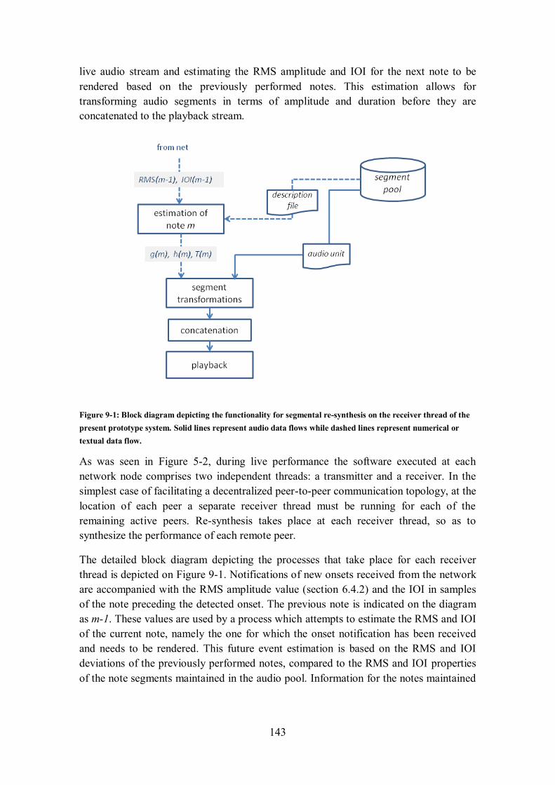
143
live audio stream and estimating the RMS amplitude and IOI for the next note to be
rendered based on the previously performed notes. This estimation allows for
transforming audio segments in terms of amplitude and duration before they are
concatenated to the playback stream.
Figure 9-1: Block diagram depicting the functionality for segmental re-synthesis on the receiver thread of the
present prototype system. Solid lines represent audio data flows while dashed lines represent numerical or
textual data flow.
As was seen in Figure 5-2, during live performance the software executed at each
network node comprises two independent threads: a transmitter and a receiver. In the
simplest case of facilitating a decentralized peer-to-peer communication topology, at the
location of each peer a separate receiver thread must be running for each of the
remaining active peers. Re-synthesis takes place at each receiver thread, so as to
synthesize the performance of each remote peer.
The detailed block diagram depicting the processes that take place for each receiver
thread is depicted on Figure 9-1. Notifications of new onsets received from the network
are accompanied with the RMS amplitude value (section 6.4.2) and the IOI in samples
of the note preceding the detected onset. The previous note is indicated on the diagram
as m-1. These values are used by a process which attempts to estimate the RMS and IOI
of the current note, namely the one for which the onset notification has been received
and needs to be rendered. This future event estimation is based on the RMS and IOI
deviations of the previously performed notes, compared to the RMS and IOI properties
of the note segments maintained in the audio pool. Information for the notes maintained
144
in the pool is derived from the corresponding performance description file (see sections
7.4.2 and 10.3.2.3).
Following, the segment that corresponds to that note is loaded from the segment pool
and transformations apply to account for the estimated RMS amplitude and duration.
Finally, a short linear cross-fade is applied between the currently rendered audio and the
first audio block of the newly loaded segment, which is subsequently appended to the
playback stream that corresponds to the performer from which the notification arrived.
In the case of multiple performers (i.e. remote peers) mixing of all synthesized streams
is performed prior to playback.
The next sub-sections describe these algorithmic processes in more detail.
9.3.1 Performance Monitoring and future event estimation
Performance monitoring provides information related to deviations in tempo and
dynamics between the live performance and the pre-segmented solo performance,
maintained in a pool of audio segments. Different segment pools correspond to the solo
recording of different performers. For this reason, a performance description-file
(section 10.3.2.3) describing the note segments that correspond to a particular performer
is parsed during the creation of each receiver thread. The information contained in this
file is maintained in memory during live performance.
Notifications of note onsets at remote ends carry information about the RMS amplitude
and the IOI of the note preceding the received onset for the live audio stream generated
at a remote network location. When receiving such a notification the deviation of that
previous note from the corresponding note in the pool of audio segments is estimated
from two ratios:
where m-1 is the index of the previous note, while the subscript live refers to the note of
the live remote stream and the subscript pool refers to the corresponding note segment
maintained in pool.
Hence, the g ratio depicts expressive deviations in music dynamics while h is related to
tempo deviations in the live performance compared to the pre-segmented solo
performance. The IOI values do not actually provide information about note durations
but only on tempo deviations, as a note may actually decay long before the occurrence
of the next onset. In fact, whether an IOI value relates to note duration is a matter of
articulation (i.e. legato, staccato, tenuto etc.) as well as a matter of timbre (e.g.
percussive instruments do not have a controllable duration).
Due to the fact that performance monitoring takes place online (i.e. causally), these
ratios are available only for the past notes. Subsequently, RMS and IOI ratios of
145
previous notes are used to predict the same ratios for the current note. In the present
implementation of the software, this prediction is based on the mean value of the
previous L notes, as:
The number of notes L over which the mean values are estimated can change or remain
constant over the duration of the piece. For instance, the mean value may be estimated
using all previous notes or it may be based on the preceding four or five notes to
account for the fact that deviations in tempo and dynamics can be constant within music
phrases, but varying over the duration of the piece. Another possibility could be to
compute a weighted mean, such as a recursive average, for which more recent notes
would have a greater influence to the estimation of future notes. For the moment the
number L=4 appeared to give satisfactory estimates.
Clearly, these techniques provide very rough estimates and are not literally predictive,
as no probabilities are involved in the computation of future estimates. A more
sophisticated mechanism for making predictions in expressive performance needs to be
incorporated. This issue is addressed in current and ongoing research efforts.
9.3.2 Segment Transformations
Based on the estimated g(m) and h(m) ratios for the next note to be rendered, i.e. the one
for which the onset was just detected, two types of transformations are applied after
loading the corresponding note from the pool of audio segments: amplitude and
duration transformations. Amplitude is transformed by multiplying the entire segment
by g(m), which is a gain or attenuation factor, depending on its value.
For duration transformations a time-domain pitch-synchronous approach that requires a
minimal amount of signal processing has been adopted. Time scaling is performed by
repeating or skipping parts of the signal having a length that corresponds to one period
of the pitch frequency (pitch synchronous transformations), while omitting the overlap-
add phase of conventional PSOLA approaches. In the present application scenario, the
pitch frequency of the segment is known before performing transformations. It is
extracted from the score file during offline segmentation and maintained in the
performance-description file (section 10.3.2.3) of the solo recording. As the target
application scenario deals with monophonic instruments the corresponding signals are
highly periodic and therefore pitch synchronous time scaling is highly appropriate.
The employed time-scaling technique is similar to PSOLA but without the overlap-add
part of the algorithm. There is one disadvantage of the proposed algorithm compared to
PSOLA, which is however not relevant for the target application scenario. The
disadvantage concerns the fact that as entire periods are added or skipped from the note,
time-scaling will not precisely provide the intended duration. It will instead have a

146
granularity that depends on the period of the periodic signal. This fact was also
addressed by the original publication introducing the PSOLA transform (Roucos and
Wilgus 1985).
In the present scenario, as the required time-scaling factor h(m) forms an approximate
estimation of the actual segment duration, imprecise time-scaling is not critical.
Moreover, omitting the overlap-add process is preferred both in respect with the
resulting computational complexity as well as in terms of the quality of the synthesized
audio stream. Future improvements of the proposed approach, such as incorporating
more sophisticated prediction algorithms and less constrained signals (i.e. in terms of
their periodicity) will require more accurate time-scaling techniques.
The rest of this section describes the algorithm for time-scaling implemented in the
present prototype system. It is important to highlight that both when time stretching (i.e.
h(m)>1) as well as when time shrinking (i.e. h(m)<1) the first part of the segment is left
unprocessed, as it is assumed to carry the initial transient of the note. As discussed in
the previous sections, initial transients should remain unprocessed to time/pitch scaling
operations due to two reasons: firstly, because they are not periodic and therefore pitch
synchronous time-domain transformations are not possible and secondly because, as
initial transients are related to the sound production mechanism of acoustic instruments,
they are important in terms of timbre perception. As they always span a small region of
the signal, time scaling initial transients would result in an unnatural audio effect.
Given an audio segment S(m) having a length of |S(m)| samples (note that |x| accounts
for the length of signal x), a time-scaling factor h(m) and a length of an initial transient
Δ, a new scaling factor h’(n), which applies only to the steady state part of the signal is
calculated as:
Intuitively, although it can also be deduced from the above formula, in the case of time
stretching, excluding the initial transient will require the remaining part to be even more
stretched (i.e. h’(n) > h(n)). In the opposite case of time shrinking less scaling will be
required on the steady state part (i.e. h’(m) < h(m)) in order to shrink by the same
amount.
The h’(m) factor will generally be a non-integer value. Achieving a final length which is
as close as possible to the desired length by repeating or omitting an integer number of
periods cannot be easily solved with algebraic calculations. Firstly, repeated or omitted
periods must be evenly distributed within the duration of the note segment in order to
maintain the overall amplitude envelope of the corresponding signal. Secondly, the
number of periods to be repeated or omitted will not necessarily be an integer multiple
of the number of existing periods in the signal. For this reason and in order to yield a
duration that is as close as possible to the intended duration, periods to be repeated or
skipped are distributed using two steps.
147
Specifically, in the case of time stretching, we define two integers as follows:
In other words α(m) is the integer/truncated (the symbol denotes integer truncation,
namely the floor() function) part of the new scaling factor h’(m), whereas β(m) is the
rounded reciprocal of the decimal part of the h’(m). Note that for any positive number
x>0, round(x) = floor(x+0.5). Then, to achieve time scaling one must repeat each
period following the initial transient of the signal α(m) times and once again at multiples
of β(m) periods of the original signal. This is shown at the top diagram of Figure 9-2.
If T(m) is the pitch period of the note segment in samples, then
denotes the number of complete (i.e. truncated) periods contained in the original
segment after the initial transient. Subsequently, the new duration of the signal can be
computed as:
In other words the new duration equals the original duration increased by the number of
extra periods.
As an example consider a note segment sampled at 44.1kHz having a length of
|S(m)|=15872 samples (i.e. 0.34 sec) with an initial transient of Δ=3584 (i.e. 81ms), a
pitch period of T(m)=100 samples (i.e. for a pitch frequency of 441Hz). A time scaling
factor of h(m)=2.23, yields a factor of h’(m)=2.59 stretching for the steady state and
therefore α(m)=2 and β(m)=2. This means that time stretching will repeat every period
(i.e. every 100 samples) following the initial transient twice and for every two of the
periods of the original signal a third repetition will be performed. As there exist
γ(m)=122 complete periods in the periodic part of the signal, the resulting segment
length will be |S’(m)|=34172, therefore yielding a scaling factor |S’(m)|/|S(m)| = 2.153,
which is 96% close to the original h(m) = 2.23.
In the case of time-shrinking (i.e. h(m) <1) a different strategy needs to be employed for
reducing the steady state up to half length, than for reducing it below half length. In the
following it is assumed that h’(n) > 0.5.
Assuming that shrinking can be achieved by removing an integer number of periods
denoted as x(m) from the periodic steady part of the segment, the following must hold:
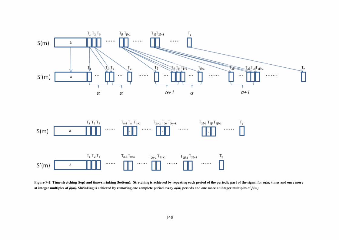
148
Figure 9-2: Time stretching (top) and time-shrinking (bottom). Stretching is achieved by repeating each period of the periodic part of the signal for α(m) times and once more
at integer multiples of β(m). Shrinking is achieved by removing one complete period every α(m) periods and one more at integer multiples of β(m).
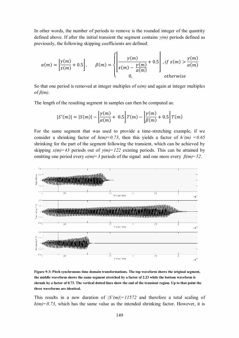
149
In other words, the number of periods to remove is the rounded integer of the quantity
defined above. If after the initial transient the segment contains γ(m) periods defined as
previously, the following skipping coefficients are defined:
So that one period is removed at integer multiples of α(m) and again at integer multiples
of β(m).
The length of the resulting segment in samples can then be computed as:
For the same segment that was used to provide a time-stretching example, if we
consider a shrinking factor of h(m)=0.73, then this yields a factor of h’(m) =0.65
shrinking for the part of the segment following the transient, which can be achieved by
skipping x(m)=43 periods out of γ(m)=122 existing periods. This can be attained by
omitting one period every α(m)=3 periods of the signal and one more every β(m)=52.
Figure 9-3: Pitch synchronous time domain transformations. The top waveform shows the original segment,
the middle waveform shows the same segment stretched by a factor of 2.23 while the bottom waveform is
shrunk by a factor of 0.73. The vertical dotted lines show the end of the transient region. Up to that point the
three waveforms are identical.
This results in a new duration of |S’(m)|=11572 and therefore a total scaling of
h(m)=0.73, which has the same value as the intended shrinking factor. However, it is
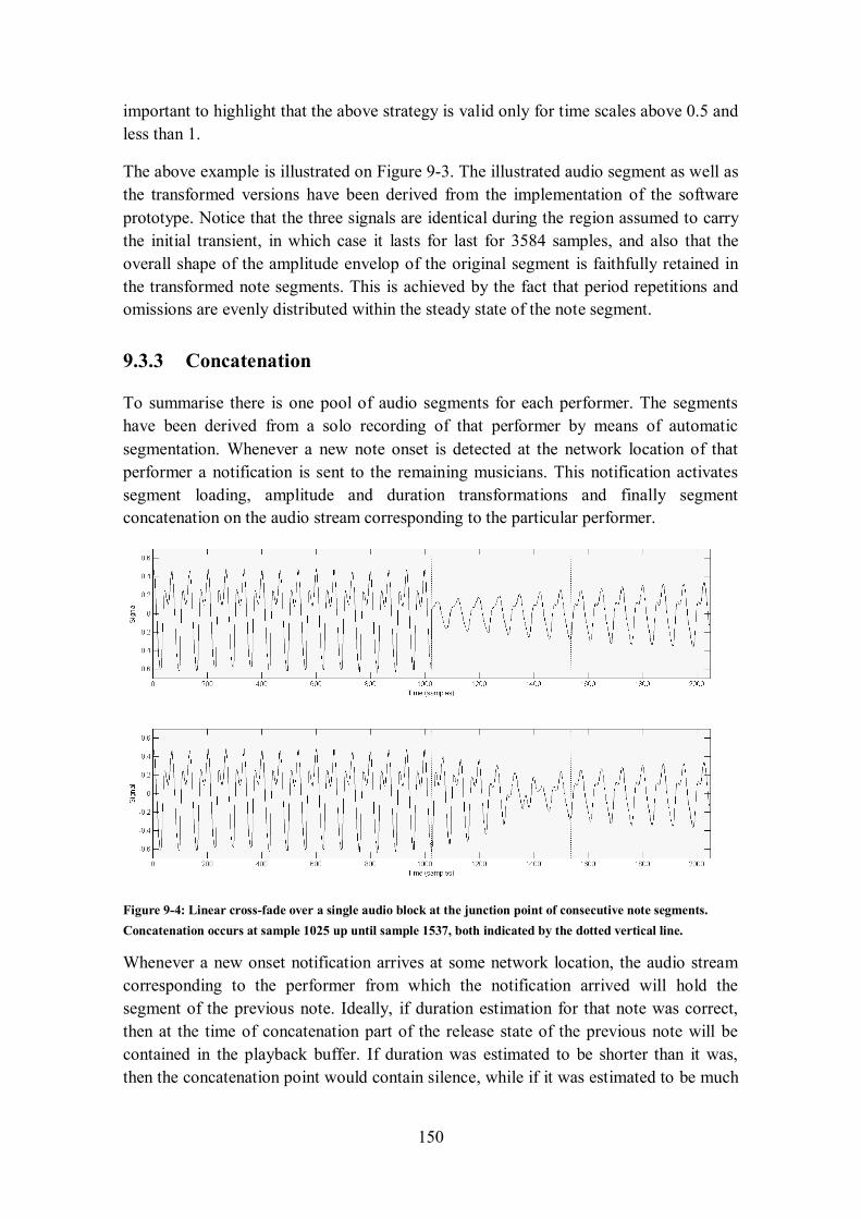
150
important to highlight that the above strategy is valid only for time scales above 0.5 and
less than 1.
The above example is illustrated on Figure 9-3. The illustrated audio segment as well as
the transformed versions have been derived from the implementation of the software
prototype. Notice that the three signals are identical during the region assumed to carry
the initial transient, in which case it lasts for last for 3584 samples, and also that the
overall shape of the amplitude envelop of the original segment is faithfully retained in
the transformed note segments. This is achieved by the fact that period repetitions and
omissions are evenly distributed within the steady state of the note segment.
9.3.3 Concatenation
To summarise there is one pool of audio segments for each performer. The segments
have been derived from a solo recording of that performer by means of automatic
segmentation. Whenever a new note onset is detected at the network location of that
performer a notification is sent to the remaining musicians. This notification activates
segment loading, amplitude and duration transformations and finally segment
concatenation on the audio stream corresponding to the particular performer.
Figure 9-4: Linear cross-fade over a single audio block at the junction point of consecutive note segments.
Concatenation occurs at sample 1025 up until sample 1537, both indicated by the dotted vertical line.
Whenever a new onset notification arrives at some network location, the audio stream
corresponding to the performer from which the notification arrived will hold the
segment of the previous note. Ideally, if duration estimation for that note was correct,
then at the time of concatenation part of the release state of the previous note will be
contained in the playback buffer. If duration was estimated to be shorter than it was,
then the concatenation point would contain silence, while if it was estimated to be much
151
longer than it actually was then the steady part of the note would be active at the
concatentation point. In all of these cases, concatenation will result in an audible
distortion perceived as a ‘click’, due to the discontinuity occurring at the junction point
of two segments.
As shown on Figure 9-4, the effect of this discontinuity is mitigated by applying a short
linear cross-fade spanning a single audio block, i.e. 512 samples of 44.1 kHz. It can be
seen that the block starting at 1025 up until 1537 contains both signals, while before and
after that block the waveforms are identical to the non-crossfaded audio streams
depicted at the top of the diagram.
As seen in section 9.2.2, offline approaches to concatenative music synthesis often
encompass more sophisticated techniques to smooth discontinuities in the range of
several audio blocks around the concatenation point. This is not possible for the current
application as the concatenation point is not known or predicted beforehand. Instead it
only becomes available when a note onset is remotely detected. Segment blending could
however expand in audio blocks following the concatenation point. Again this is not
applicable for the current scenario, because the concatenation point corresponds to the
note onset and hence the subsequent blocks most likely contain the initial transient of
the signal, which, as already elaborated in several places within this chapter, needs to
remain unprocessed in order to preserve the distinctive character of the acoustic
instrument and the performer. After all, this simple low-complexity waveform blending
solution appeared to be adequate for the target monophonic signals, as it achieves to
eliminate perceivable click distortions.
152
PART III:
IMPLEMENTATION & VALIDATION
153
10 The BoogieNet software prototype
This chapter describes the implementation details of a software prototype called
BoogieNet, which has been developed in the context of the current doctoral research.
BoogieNet provides algorithmic implementations for the functionalities of ‘Offline
Audio Segmentation’, ‘HMM Score Following’ and ‘Segmental Re-Synthesis’ as these
were presented in the previous three chapters of the dissertation. In addition to the
implementation of the algorithms, BoogieNet provides two operational modes for real-
time audio communication using notifications for detected note onsets. The first,
‘single-peer’ mode uses live audio capturing to re-synthesize the captured stream on the
same computer using onset information and segmental re-synthesis. The second, ‘udp-
peer’ operational mode permits networked musical interactions among two network
locations using HMM score following, UDP sockets and segmental re-synthesis. In this
mode, the same software application is executed at both network locations. Both peers
are capable of transmitting and at the same time receiving onset information in the form
of UDP packets. Network transmissions are initiated whenever a new note onset is
detected on the captured audio signal (e.g. from a microphone), while network reception
controls the parameters used for synthesizing the local audio stream, which are
subsequently delievered to the audio out port of the sound card. The complete prototype
is offered as an open source Application Programming Interface (API), which includes a
command line application permitting the execution of the various functional processes.
The chapter initially provides some general information on the availability of the
software prototype and a user guide explaining how to use the provided command line
application to execute the various functionalities. Then it describes important
implementation details concerning data files, data structures and the object oriented
design of the API. Finally, project dependencies and the third party libraries are
appropriately listed and cited.
10.1 Software availability
The final prototype system has been implemented in the C++ object oriented
programming language and the Linux operating system and has been thoroughly tested
on a CentOS 5 distribution. The BoogieNet prototype16
is available for download as free
and open source software under a GNU/GPL v3 license17
. The downloadable package
can be compiled and installed from source on any Linux distribution as long as the
16 http://www.teicrete.gr/diamouses/ca/phd/ 17 http://www.gnu.org/licenses/gpl.html
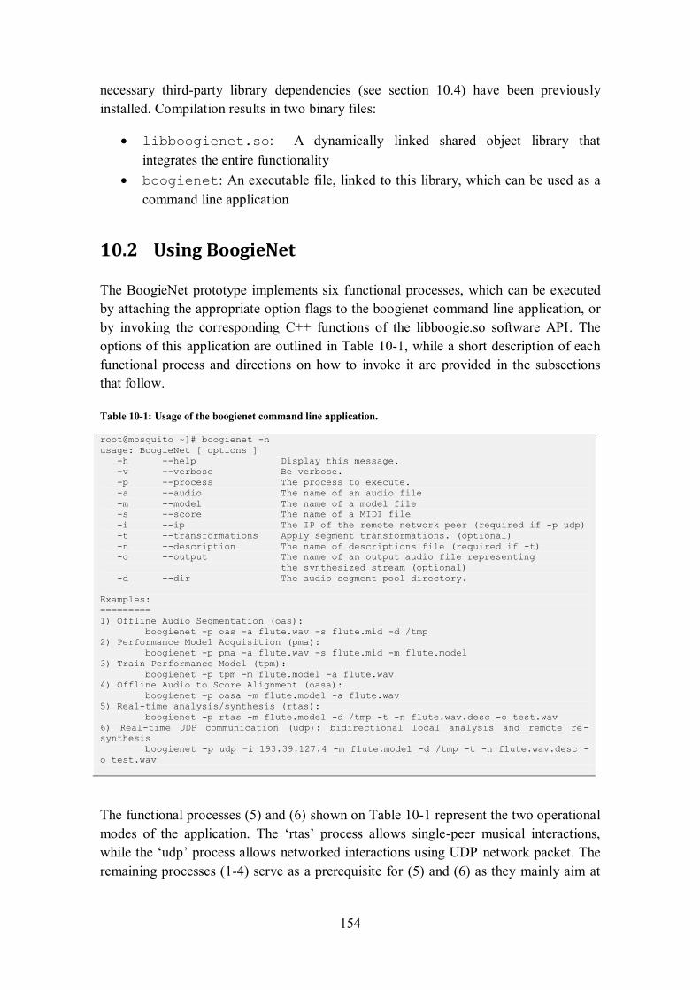
154
necessary third-party library dependencies (see section 10.4) have been previously
installed. Compilation results in two binary files:
libboogienet.so: A dynamically linked shared object library that
integrates the entire functionality
boogienet: An executable file, linked to this library, which can be used as a
command line application
10.2 Using BoogieNet
The BoogieNet prototype implements six functional processes, which can be executed
by attaching the appropriate option flags to the boogienet command line application, or
by invoking the corresponding C++ functions of the libboogie.so software API. The
options of this application are outlined in Table 10-1, while a short description of each
functional process and directions on how to invoke it are provided in the subsections
that follow.
Table 10-1: Usage of the boogienet command line application.
root@mosquito ~]# boogienet -h
usage: BoogieNet [ options ]
-h --help Display this message.
-v --verbose Be verbose.
-p --process The process to execute.
-a --audio The name of an audio file
-m --model The name of a model file
-s --score The name of a MIDI file
-i --ip The IP of the remote network peer (required if -p udp)
-t --transformations Apply segment transformations. (optional)
-n --description The name of descriptions file (required if -t)
-o --output The name of an output audio file representing
the synthesized stream (optional)
-d --dir The audio segment pool directory.
Examples:
=========
1) Offline Audio Segmentation (oas):
boogienet -p oas -a flute.wav -s flute.mid -d /tmp
2) Performance Model Acquisition (pma):
boogienet -p pma -a flute.wav -s flute.mid -m flute.model
3) Train Performance Model (tpm):
boogienet -p tpm -m flute.model -a flute.wav
4) Offline Audio to Score Alignment (oasa):
boogienet -p oasa -m flute.model -a flute.wav
5) Real-time analysis/synthesis (rtas):
boogienet -p rtas -m flute.model -d /tmp -t -n flute.wav.desc -o test.wav
6) Real-time UDP communication (udp): bidirectional local analysis and remote re-
synthesis
boogienet -p udp –i 193.39.127.4 -m flute.model -d /tmp -t -n flute.wav.desc -
o test.wav
The functional processes (5) and (6) shown on Table 10-1 represent the two operational
modes of the application. The ‘rtas’ process allows single-peer musical interactions,
while the ‘udp’ process allows networked interactions using UDP network packet. The
remaining processes (1-4) serve as a prerequisite for (5) and (6) as they mainly aim at
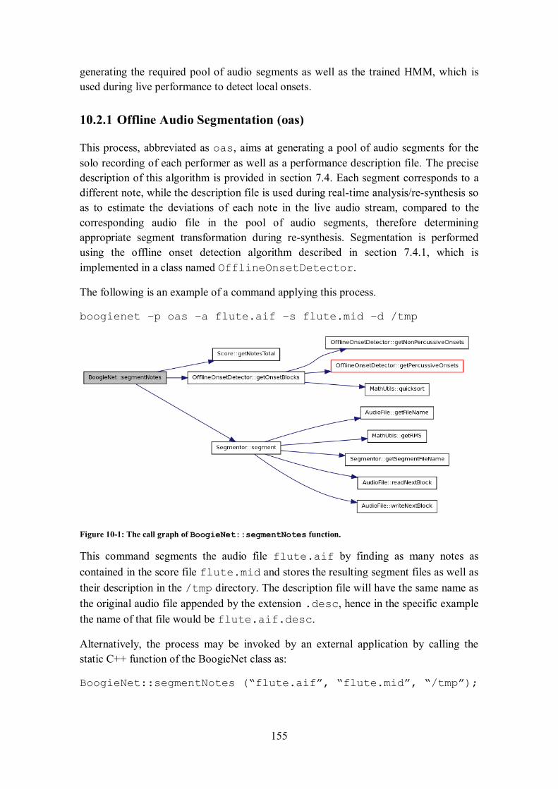
155
generating the required pool of audio segments as well as the trained HMM, which is
used during live performance to detect local onsets.
10.2.1 Offline Audio Segmentation (oas)
This process, abbreviated as oas, aims at generating a pool of audio segments for the
solo recording of each performer as well as a performance description file. The precise
description of this algorithm is provided in section 7.4. Each segment corresponds to a
different note, while the description file is used during real-time analysis/re-synthesis so
as to estimate the deviations of each note in the live audio stream, compared to the
corresponding audio file in the pool of audio segments, therefore determining
appropriate segment transformation during re-synthesis. Segmentation is performed
using the offline onset detection algorithm described in section 7.4.1, which is
implemented in a class named OfflineOnsetDetector.
The following is an example of a command applying this process.
boogienet –p oas –a flute.aif –s flute.mid –d /tmp
Figure 10-1: The call graph of BoogieNet::segmentNotes function.
This command segments the audio file flute.aif by finding as many notes as
contained in the score file flute.mid and stores the resulting segment files as well as
their description in the /tmp directory. The description file will have the same name as
the original audio file appended by the extension .desc, hence in the specific example
the name of that file would be flute.aif.desc.
Alternatively, the process may be invoked by an external application by calling the
static C++ function of the BoogieNet class as:
BoogieNet::segmentNotes (“flute.aif”, “flute.mid”, “/tmp”);
156
or equivalently invoke the commands contained within this function. Figure 10-1 shows
the call graph of this function.
10.2.2 Performance Model Acquisition (pma)
This process aims at generating an initial HMM (see section 8.3.3.2) given an audio file
and a score (MIDI) file. The model is stored in the given model filename. The process
does not apply Baum-Welch training. Instead, it generates annotations for the audio file
by applying the offline onset detection algorithm of section 7.4.1 implemented in the
class OfflineOnsetDetector and uses the class HMMAnnotator which aligns
the score to the audio file using certain heuristics. These heuristics have been described
in detail in section 8.4.1.
This initial model may be directly used for HMM decoding (offline or online) or
formerly trained with a Train Performance Model tpm process (described in the next
section) in order to refine the HMM probabilities of the initial model.
Figure 10-2: The call graph of the BoogieNet::buildHMModel function
The following is an example of a command applying the pma process.
boogienet –p pma –a flute.aif –s flute.mid –m flute.model
This command uses the flute.aif audio file and the flute.mid MIDI file to
generate an untrained model file with the name flute.model.
Alternatively, the process may be invoked by an external application by calling the
static C++ function of the BoogieNet class as:
BoogieNet::buildHMModel (“flute.aif”, “flute.mid”, “flute.model”);
or equivalently invoke the commands called within this function. Figure 10-2 depicts
the call graph of this function.
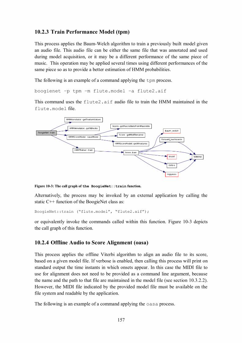
157
10.2.3 Train Performance Model (tpm)
This process applies the Baum-Welch algorithm to train a previously built model given
an audio file. This audio file can be either the same file that was annotated and used
during model acquisition, or it may be a different performance of the same piece of
music. This operation may be applied several times using different performances of the
same piece so as to provide a better estimation of HMM probabilities.
The following is an example of a command applying the tpm process.
boogienet –p tpm –m flute.model –a flute2.aif
This command uses the flute2.aif audio file to train the HMM maintained in the
flute.model file.
Figure 10-3: The call graph of the BoogieNet::train function.
Alternatively, the process may be invoked by an external application by calling the
static C++ function of the BoogieNet class as:
BoogieNet::train (“flute.model”, “flute2.aif”);
or equivalently invoke the commands called within this function. Figure 10-3 depicts
the call graph of this function.
10.2.4 Offline Audio to Score Alignment (oasa)
This process applies the offline Viterbi algorithm to align an audio file to its score,
based on a given model file. If verbose is enabled, then calling this process will print on
standard output the time instants in which onsets appear. In this case the MIDI file to
use for alignment does not need to be provided as a command line argument, because
the name and the path to that file are maintained in the model file (see section 10.3.2.2).
However, the MIDI file indicated by the provided model file must be available on the
file system and readable by the application.
The following is an example of a command applying the oasa process.
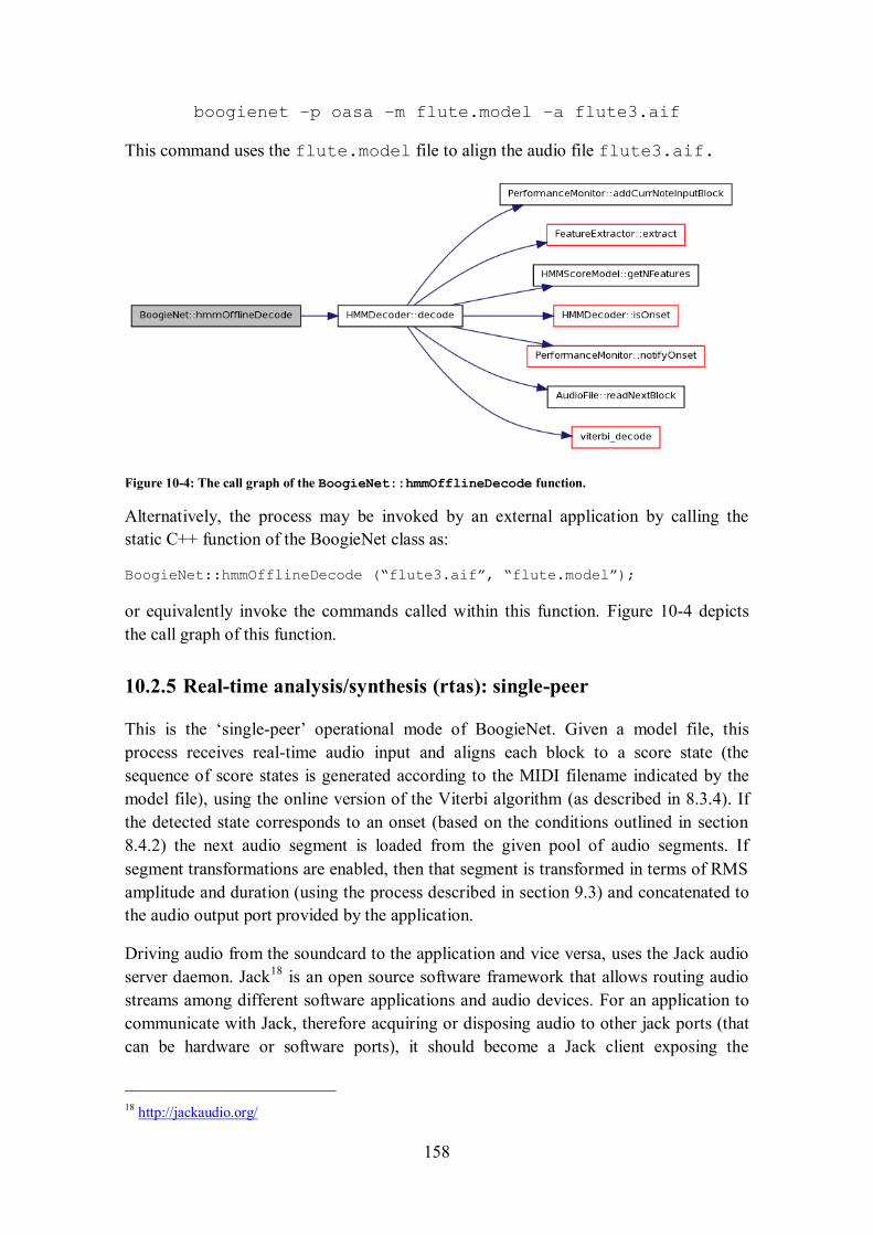
158
boogienet –p oasa –m flute.model –a flute3.aif
This command uses the flute.model file to align the audio file flute3.aif.
Figure 10-4: The call graph of the BoogieNet::hmmOfflineDecode function.
Alternatively, the process may be invoked by an external application by calling the
static C++ function of the BoogieNet class as:
BoogieNet::hmmOfflineDecode (“flute3.aif”, “flute.model”);
or equivalently invoke the commands called within this function. Figure 10-4 depicts
the call graph of this function.
10.2.5 Real-time analysis/synthesis (rtas): single-peer
This is the ‘single-peer’ operational mode of BoogieNet. Given a model file, this
process receives real-time audio input and aligns each block to a score state (the
sequence of score states is generated according to the MIDI filename indicated by the
model file), using the online version of the Viterbi algorithm (as described in 8.3.4). If
the detected state corresponds to an onset (based on the conditions outlined in section
8.4.2) the next audio segment is loaded from the given pool of audio segments. If
segment transformations are enabled, then that segment is transformed in terms of RMS
amplitude and duration (using the process described in section 9.3) and concatenated to
the audio output port provided by the application.
Driving audio from the soundcard to the application and vice versa, uses the Jack audio
server daemon. Jack18
is an open source software framework that allows routing audio
streams among different software applications and audio devices. For an application to
communicate with Jack, therefore acquiring or disposing audio to other jack ports (that
can be hardware or software ports), it should become a Jack client exposing the
18 http://jackaudio.org/
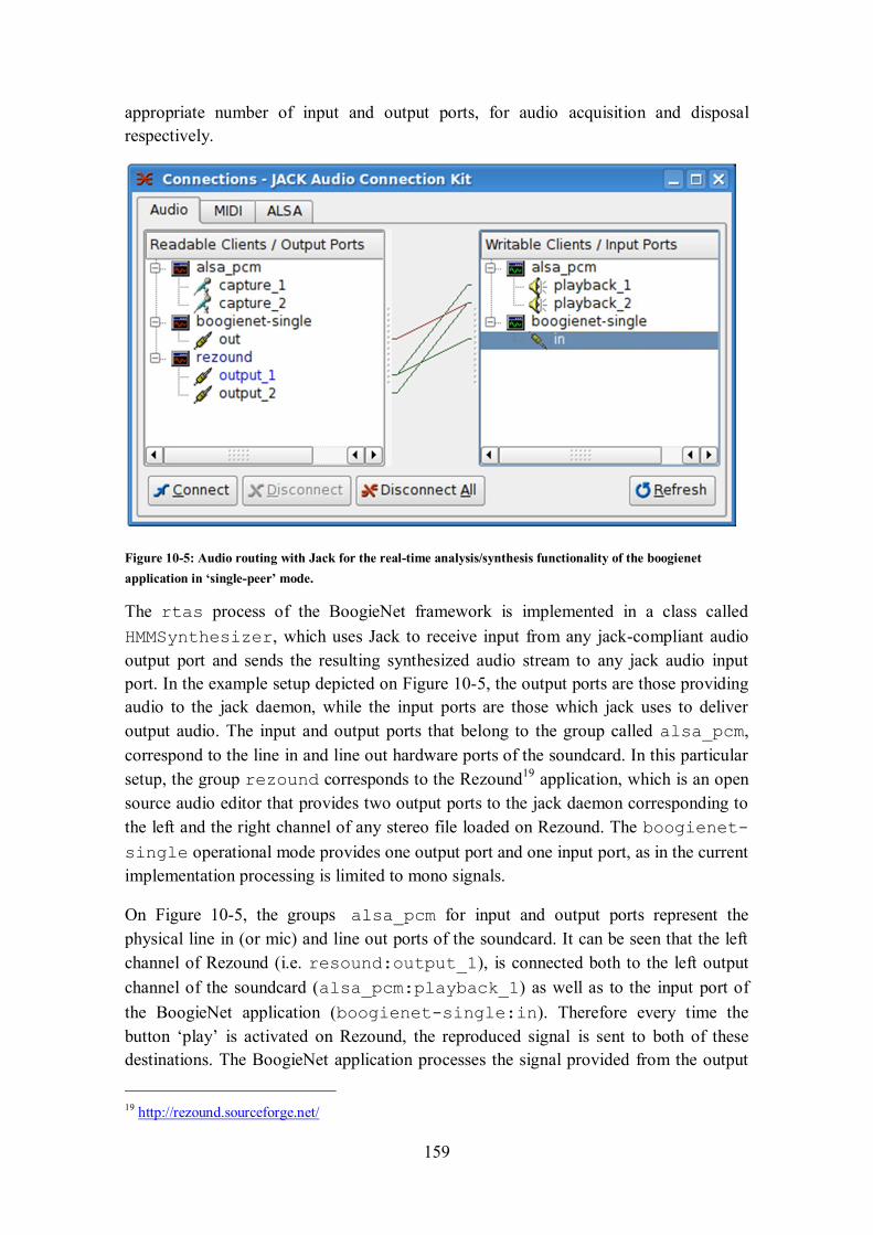
159
appropriate number of input and output ports, for audio acquisition and disposal
respectively.
Figure 10-5: Audio routing with Jack for the real-time analysis/synthesis functionality of the boogienet
application in ‘single-peer’ mode.
The rtas process of the BoogieNet framework is implemented in a class called
HMMSynthesizer, which uses Jack to receive input from any jack-compliant audio
output port and sends the resulting synthesized audio stream to any jack audio input
port. In the example setup depicted on Figure 10-5, the output ports are those providing
audio to the jack daemon, while the input ports are those which jack uses to deliver
output audio. The input and output ports that belong to the group called alsa_pcm,
correspond to the line in and line out hardware ports of the soundcard. In this particular
setup, the group rezound corresponds to the Rezound19
application, which is an open
source audio editor that provides two output ports to the jack daemon corresponding to
the left and the right channel of any stereo file loaded on Rezound. The boogienet-
single operational mode provides one output port and one input port, as in the current
implementation processing is limited to mono signals.
On Figure 10-5, the groups alsa_pcm for input and output ports represent the
physical line in (or mic) and line out ports of the soundcard. It can be seen that the left
channel of Rezound (i.e. resound:output_1), is connected both to the left output
channel of the soundcard (alsa_pcm:playback_1) as well as to the input port of
the BoogieNet application (boogienet-single:in). Therefore every time the
button ‘play’ is activated on Rezound, the reproduced signal is sent to both of these
destinations. The BoogieNet application processes the signal provided from the output
19 http://rezound.sourceforge.net/
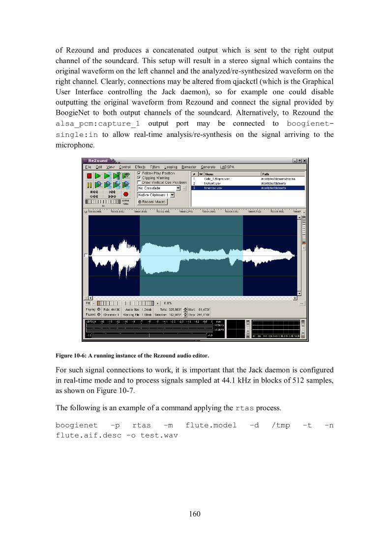
160
of Rezound and produces a concatenated output which is sent to the right output
channel of the soundcard. This setup will result in a stereo signal which contains the
original waveform on the left channel and the analyzed/re-synthesized waveform on the
right channel. Clearly, connections may be altered from qjackctl (which is the Graphical
User Interface controlling the Jack daemon), so for example one could disable
outputting the original waveform from Rezound and connect the signal provided by
BoogieNet to both output channels of the soundcard. Alternatively, to Rezound the
alsa_pcm:capture_1 output port may be connected to boogienet-
single:in to allow real-time analysis/re-synthesis on the signal arriving to the
microphone.
Figure 10-6: A running instance of the Rezound audio editor.
For such signal connections to work, it is important that the Jack daemon is configured
in real-time mode and to process signals sampled at 44.1 kHz in blocks of 512 samples,
as shown on Figure 10-7.
The following is an example of a command applying the rtas process.
boogienet –p rtas –m flute.model –d /tmp –t –n
flute.aif.desc –o test.wav
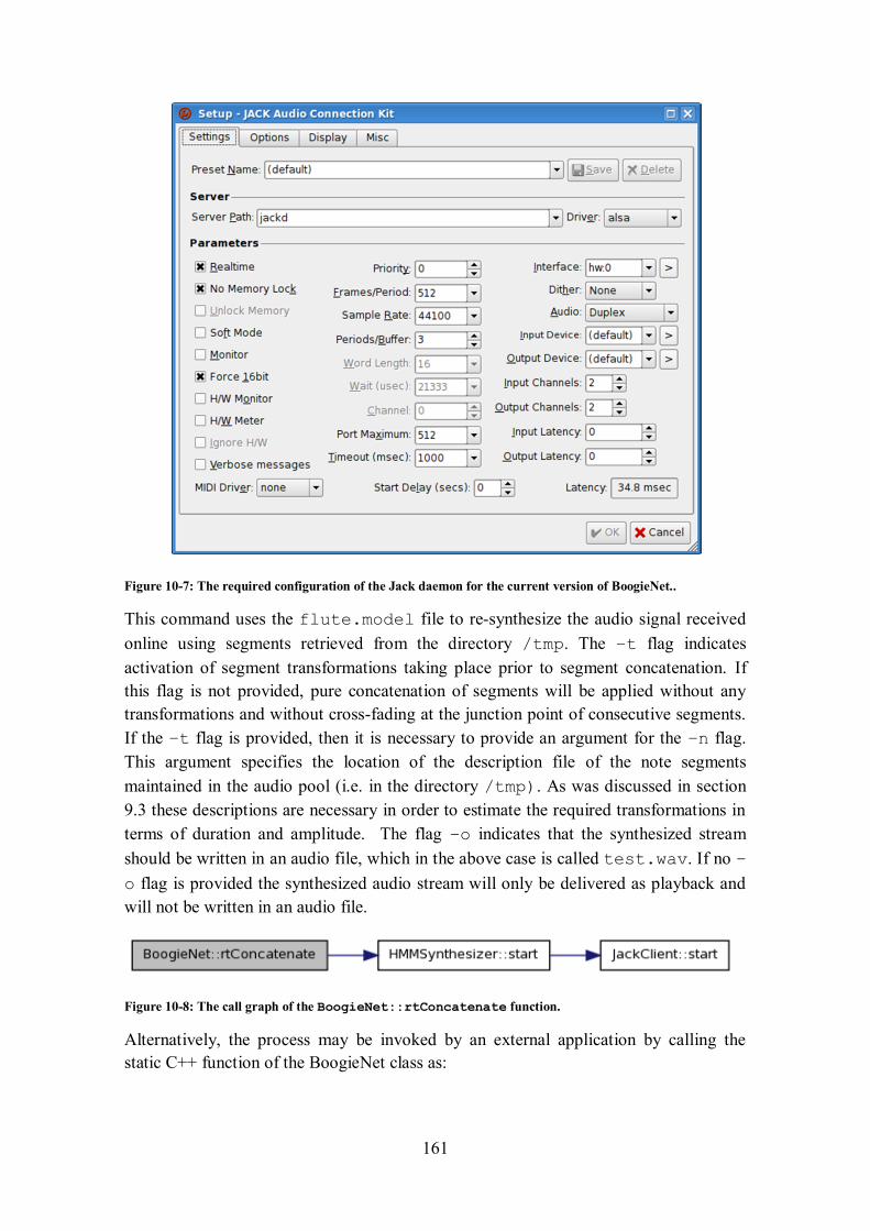
161
Figure 10-7: The required configuration of the Jack daemon for the current version of BoogieNet..
This command uses the flute.model file to re-synthesize the audio signal received
online using segments retrieved from the directory /tmp. The –t flag indicates
activation of segment transformations taking place prior to segment concatenation. If
this flag is not provided, pure concatenation of segments will be applied without any
transformations and without cross-fading at the junction point of consecutive segments.
If the –t flag is provided, then it is necessary to provide an argument for the –n flag.
This argument specifies the location of the description file of the note segments
maintained in the audio pool (i.e. in the directory /tmp). As was discussed in section
9.3 these descriptions are necessary in order to estimate the required transformations in
terms of duration and amplitude. The flag –o indicates that the synthesized stream
should be written in an audio file, which in the above case is called test.wav. If no –
o flag is provided the synthesized audio stream will only be delivered as playback and
will not be written in an audio file.
Figure 10-8: The call graph of the BoogieNet::rtConcatenate function.
Alternatively, the process may be invoked by an external application by calling the
static C++ function of the BoogieNet class as:
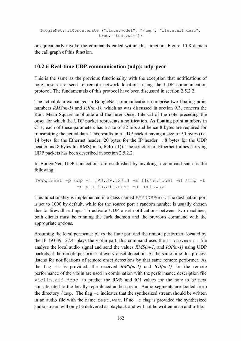
162
BoogieNet::rtConcatenate (“flute.model”, “/tmp”, “flute.aif.desc”,
true, “test.wav”);
or equivalently invoke the commands called within this function. Figure 10-8 depicts
the call graph of this function.
10.2.6 Real-time UDP communication (udp): udp-peer
This is the same as the previous functionality with the exception that notifications of
note onsets are send to remote network locations using the UDP communication
protocol. The fundamentals of this protocol have been discussed in section 2.5.2.2.
The actual data exchanged in BoogieNet communications comprise two floating point
numbers RMS(m-1) and IOI(m-1), which as was discussed in section 9.3, concern the
Root Mean Square amplitude and the Inter Onset Interval of the note preceding the
onset for which the UDP packet represents a notification. As floating point numbers in
C++, each of these parameters has a size of 32 bits and hence 8 bytes are required for
transmitting the actual data. This results in a UDP packet having a size of 50 bytes (i.e.
14 bytes for the Ethernet header, 20 bytes for the IP header , 8 bytes for the UDP
header and 8 bytes for RMS(m-1), IOI(m-1)). The structure of Ethernet frames carrying
UDP packets has been described in section 2.5.2.2.
In BoogieNet, UDP connections are established by invoking a command such as the
following:
boogienet –p udp –i 193.39.127.4 –m flute.model –d /tmp –t
–n violin.aif.desc –o test.wav
This functionality is implemented in a class named HMMUDPPeer. The destination port
is set to 1000 by default, while for the source port a random number is usually chosen
due to firewall settings. To activate UDP onset notifications between two machines,
both clients must be running the Jack daemon and the previous command with the
appropriate options.
Assuming the local performer plays the flute part and the remote performer, located by
the IP 193.39.127.4, plays the violin part, this command uses the flute.model file
analyse the local audio signal and send the values RMS(m-1) and IOI(m-1) using UDP
packets at the remote performer at every onset detection. At the same time this process
listens for notifications of remote onset detections by that same remote performer. As
the flag –t is provided, the received RMS(m-1) and IOI(m-1) for the remote
performance of the violin are used in combination with the performance description file
violin.aif.desc to predict the RMS and IOI values for the note to be next
concatenated to the locally reproduced audio stream. Audio segments are loaded from
the directory /tmp. The flag –o indicates that the synthesized stream should be written
in an audio file with the name test.wav. If no –o flag is provided the synthesized
audio stream will only be delivered as playback and will not be written in an audio file.
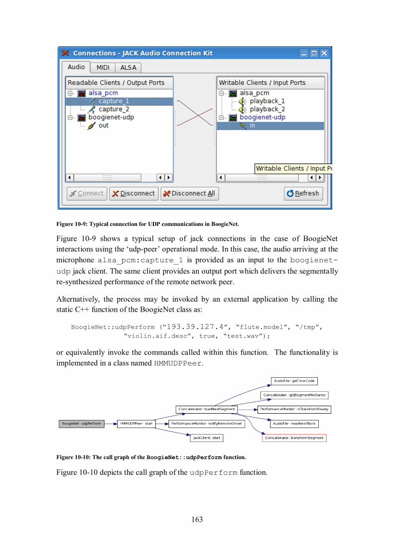
163
Figure 10-9: Typical connection for UDP communications in BoogieNet.
Figure 10-9 shows a typical setup of jack connections in the case of BoogieNet
interactions using the ‘udp-peer’ operational mode. In this case, the audio arriving at the
microphone alsa_pcm:capture_1 is provided as an input to the boogienet-
udp jack client. The same client provides an output port which delivers the segmentally
re-synthesized performance of the remote network peer.
Alternatively, the process may be invoked by an external application by calling the
static C++ function of the BoogieNet class as:
BoogieNet::udpPerform (“193.39.127.4”, “flute.model”, “/tmp”,
“violin.aif.desc”, true, “test.wav”);
or equivalently invoke the commands called within this function. The functionality is
implemented in a class named HMMUDPPeer.
Figure 10-10: The call graph of the BoogieNet::udpPerform function.
Figure 10-10 depicts the call graph of the udpPerform function.
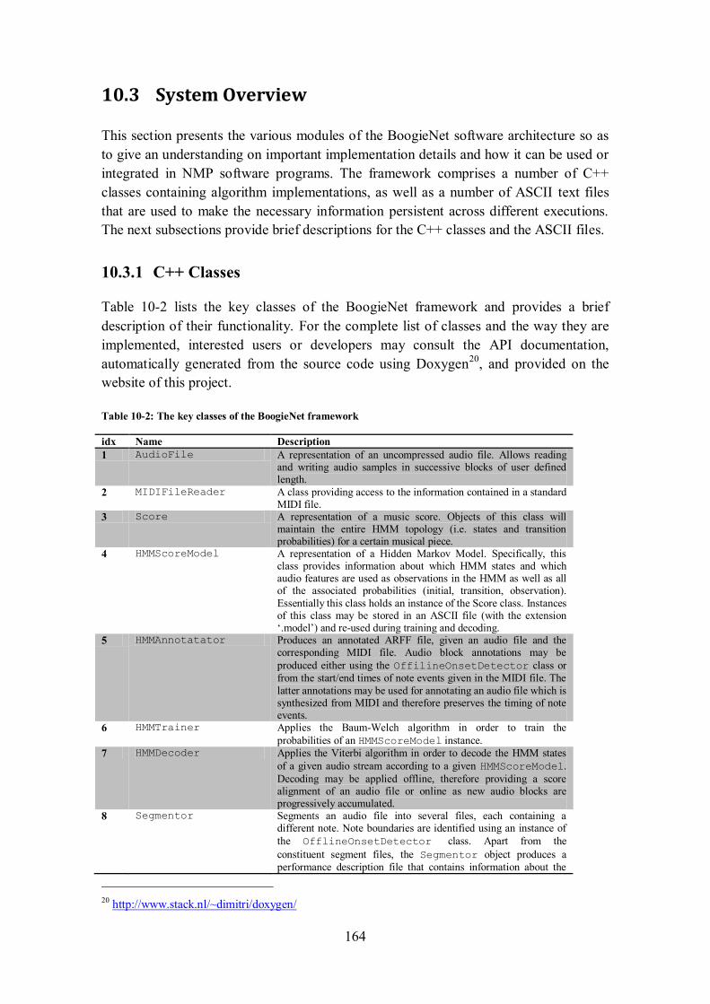
164
10.3 System Overview
This section presents the various modules of the BoogieNet software architecture so as
to give an understanding on important implementation details and how it can be used or
integrated in NMP software programs. The framework comprises a number of C++
classes containing algorithm implementations, as well as a number of ASCII text files
that are used to make the necessary information persistent across different executions.
The next subsections provide brief descriptions for the C++ classes and the ASCII files.
10.3.1 C++ Classes
Table 10-2 lists the key classes of the BoogieNet framework and provides a brief
description of their functionality. For the complete list of classes and the way they are
implemented, interested users or developers may consult the API documentation,
automatically generated from the source code using Doxygen20
, and provided on the
website of this project.
Table 10-2: The key classes of the BoogieNet framework
idx Name Description
1 AudioFile A representation of an uncompressed audio file. Allows reading and writing audio samples in successive blocks of user defined length.
2 MIDIFileReader A class providing access to the information contained in a standard MIDI file.
3 Score A representation of a music score. Objects of this class will maintain the entire HMM topology (i.e. states and transition probabilities) for a certain musical piece.
4 HMMScoreModel A representation of a Hidden Markov Model. Specifically, this class provides information about which HMM states and which audio features are used as observations in the HMM as well as all of the associated probabilities (initial, transition, observation).
Essentially this class holds an instance of the Score class. Instances of this class may be stored in an ASCII file (with the extension ‘.model’) and re-used during training and decoding.
5 HMMAnnotatator Produces an annotated ARFF file, given an audio file and the corresponding MIDI file. Audio block annotations may be
produced either using the OffilineOnsetDetector class or
from the start/end times of note events given in the MIDI file. The
latter annotations may be used for annotating an audio file which is synthesized from MIDI and therefore preserves the timing of note events.
6 HMMTrainer Applies the Baum-Welch algorithm in order to train the
probabilities of an HMMScoreModel instance.
7 HMMDecoder Applies the Viterbi algorithm in order to decode the HMM states
of a given audio stream according to a given HMMScoreModel.
Decoding may be applied offline, therefore providing a score alignment of an audio file or online as new audio blocks are progressively accumulated.
8 Segmentor Segments an audio file into several files, each containing a different note. Note boundaries are identified using an instance of
the OfflineOnsetDetector class. Apart from the
constituent segment files, the Segmentor object produces a
performance description file that contains information about the
20 http://www.stack.nl/~dimitri/doxygen/

165
length, the RMS amplitude and the pitch of the note contained in each segment. These descriptions are used during synthesis to apply segment transformations prior to concatenation.
9 OfflineOnsetDetector Detects the location of note onsets in an audio waveform by applying the blind onset detection algorithm provided in section 7.4.1.
10 PitchDetector Provides a C++ implementation of the Maddox and Larson (2005) algorithm for pitch detection using wavelets.
11 Concatenator Instances of this class perform segmental synthesis by loading the audio files that correspond to note segments. This class is invoked
by the HMMSynthesizer everytime new audio data must be
sent to the output. The Concatenator will load a new audio
segment every time it is notified for the occurrence of a new onset. If amplitude and duration transformations are enabled it perform
then when loading a new audio segment. If no onset occurs, it will provide the next audio block of the current segment to the
HMMSynthesizer object.
12 HMMSynthesizer It performs segmental analysis and re-synthesis based on audio blocks received in real-time. It holds an instance of an
HMMDecoder as well as an instance of the Concatenator
class. The HMMSynthesizer class is a subclass of a Jack Client,
exposing an audio input as well as an audio output port. It receives input from any Jack output port such as the microphone or line in of the sound card or any jack compliant audio player (e.g.
JackTrip, Audacity, rezound) and it calls the HMMDecoder class
to decode the received audio block and find its score position as the corresponding HMM state. If that state corresponds to a note
onset it instructs its Concatenator object to load the next
segment from the pool of audio segments, otherwise it asks for the next audio block from the current possibly transformed audio segment in order to forward it to the line out of the audio device.
HMMSynthesizer may additionally save the concatenated audio
to a sound file, if created by calling the appropriate constructor.
13 HMMUDPPeer This is similar to the HMMSynthesizer class and it additionally
implements UDP communications. It holds an instance of an
HMMDecoder and an instance of the Concatenator class and
it is a subclass of JackClient exposing one input and one
output audio port to Jack. At the same time this class opens the 1000 UDP ports for listening, hence waiting to receive remote onset notifications. Every time an onset is detected on the local performance a notification is sent to port 1000 of the remote peer identified by the provided IP address.
14 FeatureExtractor Extracts the requested audio features either offline (i.e. from an audio file) or online (i.e. from successive audio blocks).
15 SpectrumAnalyser Performs the Fourier transform of a given audio segment. This is an abstract class subclassed by different classes implementing different parameterisations of the STFT, which are described in section 6.3.
16 PerformanceMonitor This class loads a performance description file and gets notified by
the HMMDecoder every time a new onset occurs. For every new
note it maintains its divergence from the corresponding audio
segment in the pool of audio segments in terms of duration (in samples) and RMS amplitude. These divergences are made
available to the Concatenator object which then attempts to
predict the divergence of an upcoming note when its onset occurs.
17 BoogieNet This is a main class provided for testing purposes. It allows executing the functionalities of offline audio segmentation, performance model acquisition, training a performance model,
performing offline audio-to-score alignment using an HMM and finally, real-time analysis re-synthesis. This main class when executed with the appropriate flags allows testing the corresponding functionalities in a stand-alone application. In real-time operation it requires communication with the jack audio daemon.
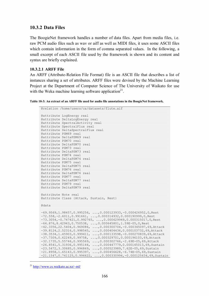
166
10.3.2 Data Files
The BoogieNet framework handles a number of data files. Apart from media files, i.e.
raw PCM audio files such as wav or aiff as well as MIDI files, it uses some ASCII files
which contain information in the form of comma separated values. In the following, a
small excerpt of each ASCII file used by the framework is shown and its content and
syntax are briefly explained.
10.3.2.1 ARFF File
An ARFF (Attribute-Relation File Format) file is an ASCII file that describes a list of
instances sharing a set of attributes. ARFF files were devised by the Machine Learning
Project at the Department of Computer Science of The University of Waikato for use
with the Weka machine learning software application21
.
Table 10-3: An extract of an ARFF file used for audio file annotations in the BoogieNet framework.
@relation /home/users/ca/datasets/flute.aif
@attribute LogEnergy real
@attribute DeltaLogEnergy real
@attribute SpectralActivity real
@attribute SpectralFlux real
@attribute DeltaSpectralFlux real
@attribute PSM69 real
@attribute DeltaPSM69 real
@attribute PSM70 real
@attribute DeltaPSM70 real
@attribute PSM73 real
@attribute DeltaPSM73 real
@attribute PSM74 real
@attribute DeltaPSM74 real
@attribute PSM75 real
@attribute DeltaPSM75 real
@attribute PSM76 real
@attribute DeltaPSM76 real
@attribute PSM77 real
@attribute DeltaPSM77 real
@attribute PSM79 real
@attribute DeltaPSM79 real
@attribute Note real
@attribute Class {Attack, Sustain, Rest}
@data
-69.9569,1.98457,0.995256, ...,0.000123933,-0.000426952,0,Rest
-72.558,-2.6011,0.991661, ...,0.000314932,0.000190999,0,Rest
-73.3054,-0.747421,0.992765, ...,0.000629949,0.000315017,0,Rest
-64.876,8.42943,0.750538, ...,0.000645801,1.59E-05,0,Rest
-42.3356,22.5404,0.969086, ...,0.000300704,-0.000345097,69,Attack
-39.8124,2.52316,0.998545, ...,0.000404436,0.000103732,69,Attack
-38.3534,1.45903,0.999411, ...,0.000133598,-0.000270839,69,Attack
-37.7309,0.62249,0.99758, ...,0.000329701,0.000196103,69,Attack
-32.1735,5.55746,0.995569, ...,0.000302766,-2.69E-05,69,Attack
-26.8541,5.31936,0.995144, ...,0.000447779,0.000145013,69,Sustain
-23.5472,3.30685,0.994849, ...,0.000523989,7.62E-05,69,Sustain
-21.8958,1.65143,0.995397, ...,0.000456628,-6.74E-05,69,Sustain
-21.1547,0.741125,0.996622, ...,0.000330994,-0.000125634,69,Sustain
21 http://www.cs.waikato.ac.nz/~ml/
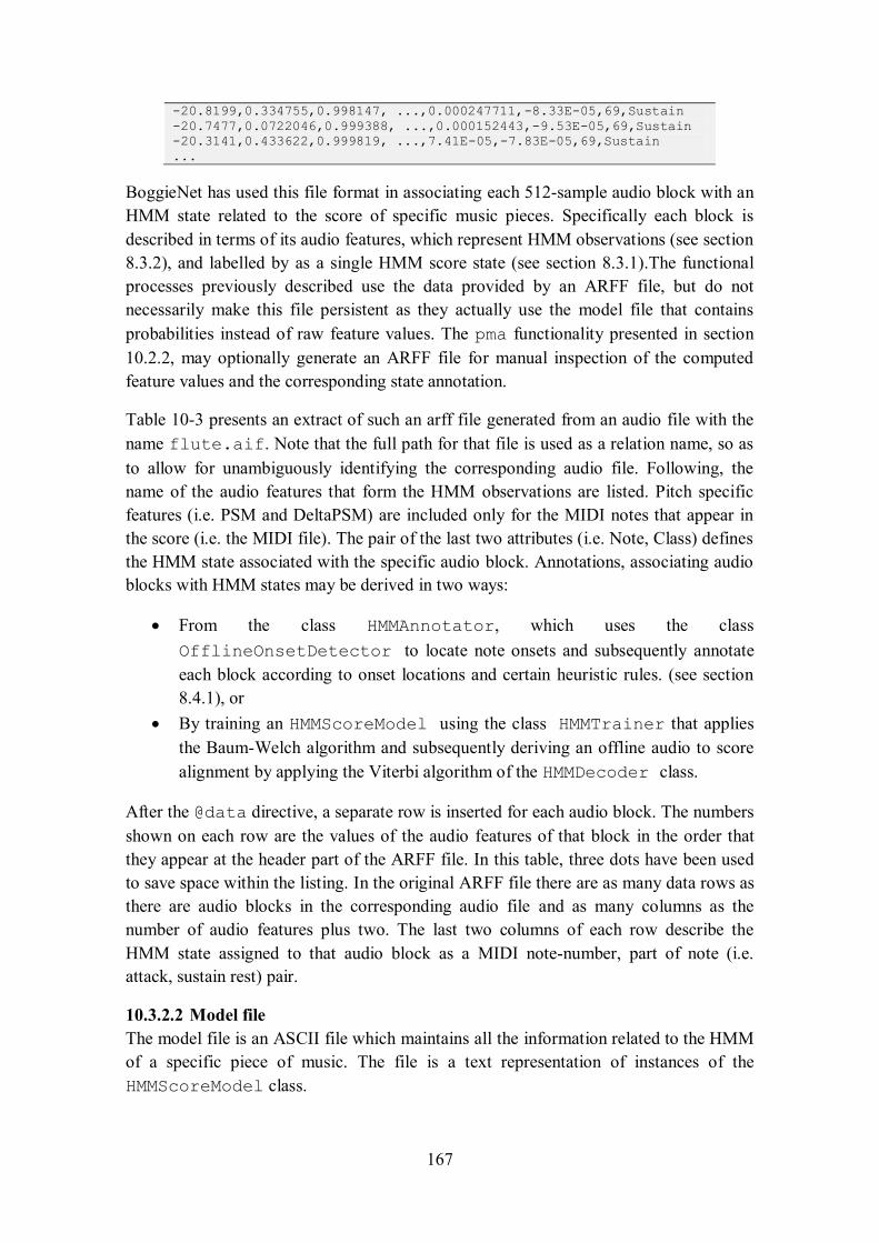
167
-20.8199,0.334755,0.998147, ...,0.000247711,-8.33E-05,69,Sustain
-20.7477,0.0722046,0.999388, ...,0.000152443,-9.53E-05,69,Sustain
-20.3141,0.433622,0.999819, ...,7.41E-05,-7.83E-05,69,Sustain
...
BoggieNet has used this file format in associating each 512-sample audio block with an
HMM state related to the score of specific music pieces. Specifically each block is
described in terms of its audio features, which represent HMM observations (see section
8.3.2), and labelled by as a single HMM score state (see section 8.3.1).The functional
processes previously described use the data provided by an ARFF file, but do not
necessarily make this file persistent as they actually use the model file that contains
probabilities instead of raw feature values. The pma functionality presented in section
10.2.2, may optionally generate an ARFF file for manual inspection of the computed
feature values and the corresponding state annotation.
Table 10-3 presents an extract of such an arff file generated from an audio file with the
name flute.aif. Note that the full path for that file is used as a relation name, so as
to allow for unambiguously identifying the corresponding audio file. Following, the
name of the audio features that form the HMM observations are listed. Pitch specific
features (i.e. PSM and DeltaPSM) are included only for the MIDI notes that appear in
the score (i.e. the MIDI file). The pair of the last two attributes (i.e. Note, Class) defines
the HMM state associated with the specific audio block. Annotations, associating audio
blocks with HMM states may be derived in two ways:
From the class HMMAnnotator, which uses the class
OfflineOnsetDetector to locate note onsets and subsequently annotate
each block according to onset locations and certain heuristic rules. (see section
8.4.1), or
By training an HMMScoreModel using the class HMMTrainer that applies
the Baum-Welch algorithm and subsequently deriving an offline audio to score
alignment by applying the Viterbi algorithm of the HMMDecoder class.
After the @data directive, a separate row is inserted for each audio block. The numbers
shown on each row are the values of the audio features of that block in the order that
they appear at the header part of the ARFF file. In this table, three dots have been used
to save space within the listing. In the original ARFF file there are as many data rows as
there are audio blocks in the corresponding audio file and as many columns as the
number of audio features plus two. The last two columns of each row describe the
HMM state assigned to that audio block as a MIDI note-number, part of note (i.e.
attack, sustain rest) pair.
10.3.2.2 Model file
The model file is an ASCII file which maintains all the information related to the HMM
of a specific piece of music. The file is a text representation of instances of the
HMMScoreModel class.
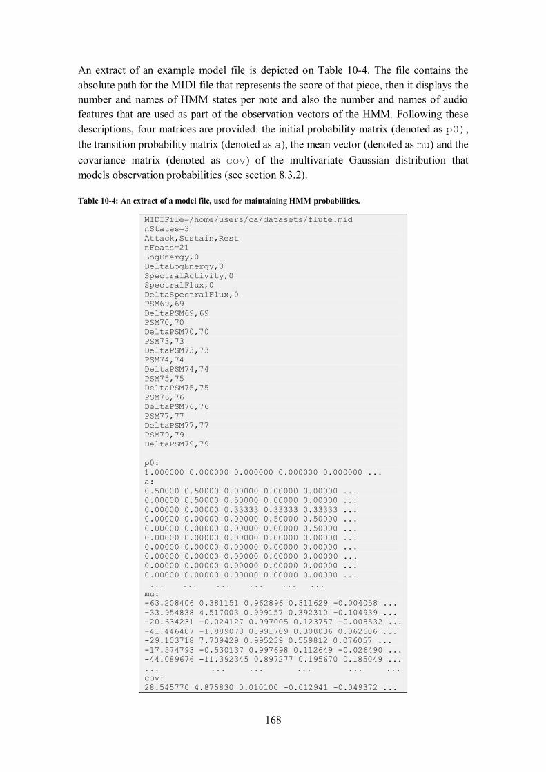
168
An extract of an example model file is depicted on Table 10-4. The file contains the
absolute path for the MIDI file that represents the score of that piece, then it displays the
number and names of HMM states per note and also the number and names of audio
features that are used as part of the observation vectors of the HMM. Following these
descriptions, four matrices are provided: the initial probability matrix (denoted as p0),
the transition probability matrix (denoted as a), the mean vector (denoted as mu) and the
covariance matrix (denoted as cov) of the multivariate Gaussian distribution that
models observation probabilities (see section 8.3.2).
Table 10-4: An extract of a model file, used for maintaining HMM probabilities.
MIDIFile=/home/users/ca/datasets/flute.mid
nStates=3
Attack,Sustain,Rest
nFeats=21
LogEnergy,0
DeltaLogEnergy,0
SpectralActivity,0
SpectralFlux,0
DeltaSpectralFlux,0
PSM69,69
DeltaPSM69,69
PSM70,70
DeltaPSM70,70
PSM73,73
DeltaPSM73,73
PSM74,74
DeltaPSM74,74
PSM75,75
DeltaPSM75,75
PSM76,76
DeltaPSM76,76
PSM77,77
DeltaPSM77,77
PSM79,79
DeltaPSM79,79
p0:
1.000000 0.000000 0.000000 0.000000 0.000000 ...
a:
0.50000 0.50000 0.00000 0.00000 0.00000 ...
0.00000 0.50000 0.50000 0.00000 0.00000 ...
0.00000 0.00000 0.33333 0.33333 0.33333 ...
0.00000 0.00000 0.00000 0.50000 0.50000 ...
0.00000 0.00000 0.00000 0.00000 0.50000 ...
0.00000 0.00000 0.00000 0.00000 0.00000 ...
0.00000 0.00000 0.00000 0.00000 0.00000 ...
0.00000 0.00000 0.00000 0.00000 0.00000 ...
0.00000 0.00000 0.00000 0.00000 0.00000 ...
0.00000 0.00000 0.00000 0.00000 0.00000 ...
... ... ... ... ... ...
mu:
-63.208406 0.381151 0.962896 0.311629 -0.004058 ...
-33.954838 4.517003 0.999157 0.392310 -0.104939 ...
-20.634231 -0.024127 0.997005 0.123757 -0.008532 ...
-41.446407 -1.889078 0.991709 0.308036 0.062606 ...
-29.103718 7.709429 0.995239 0.559812 0.076057 ...
-17.574793 -0.530137 0.997698 0.112649 -0.026490 ...
-44.089676 -11.392345 0.897277 0.195670 0.185049 ...
... ... ... ... ... ...
cov:
28.545770 4.875830 0.010100 -0.012941 -0.049372 ...
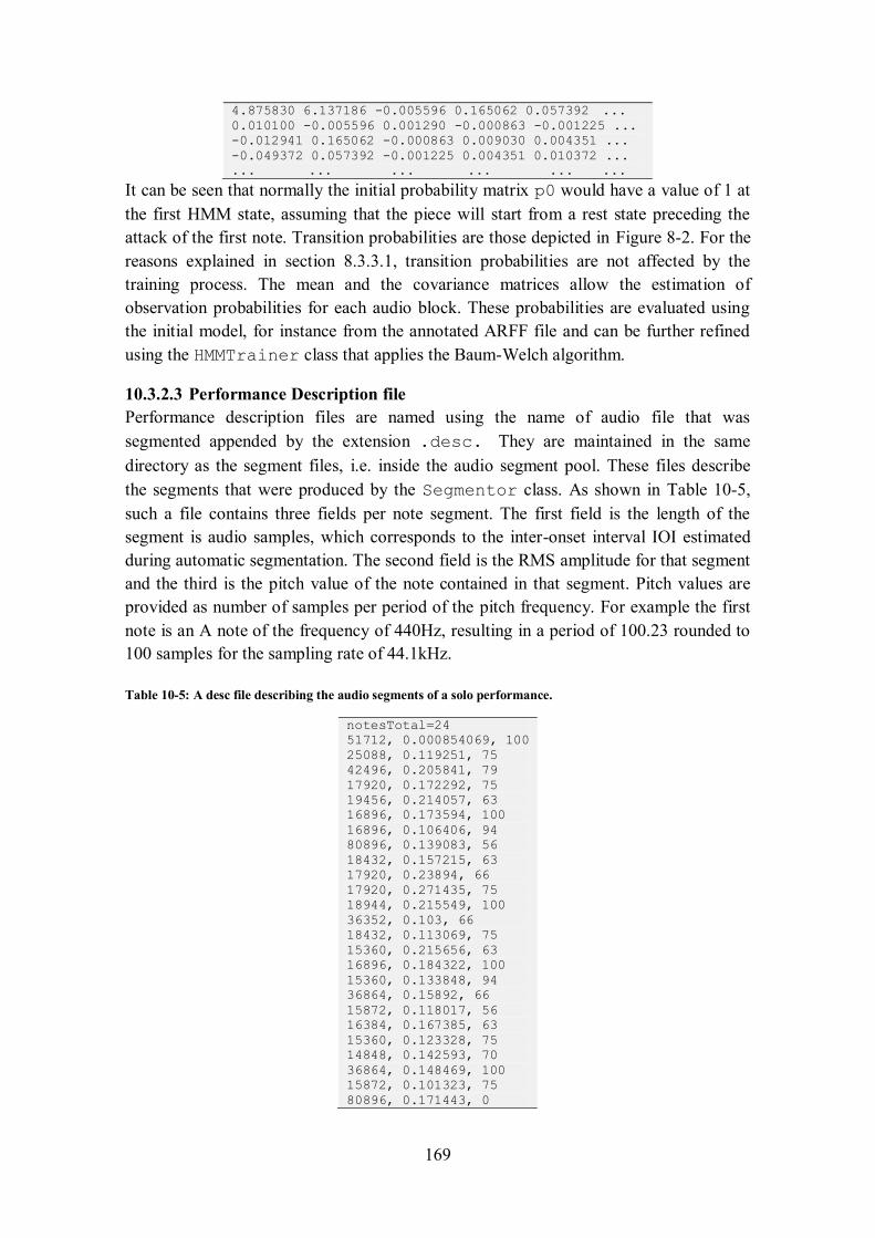
169
4.875830 6.137186 -0.005596 0.165062 0.057392 ...
0.010100 -0.005596 0.001290 -0.000863 -0.001225 ...
-0.012941 0.165062 -0.000863 0.009030 0.004351 ...
-0.049372 0.057392 -0.001225 0.004351 0.010372 ...
... ... ... ... ... ...
It can be seen that normally the initial probability matrix p0 would have a value of 1 at
the first HMM state, assuming that the piece will start from a rest state preceding the
attack of the first note. Transition probabilities are those depicted in Figure 8-2. For the
reasons explained in section 8.3.3.1, transition probabilities are not affected by the
training process. The mean and the covariance matrices allow the estimation of
observation probabilities for each audio block. These probabilities are evaluated using
the initial model, for instance from the annotated ARFF file and can be further refined
using the HMMTrainer class that applies the Baum-Welch algorithm.
10.3.2.3 Performance Description file
Performance description files are named using the name of audio file that was
segmented appended by the extension .desc. They are maintained in the same
directory as the segment files, i.e. inside the audio segment pool. These files describe
the segments that were produced by the Segmentor class. As shown in Table 10-5,
such a file contains three fields per note segment. The first field is the length of the
segment is audio samples, which corresponds to the inter-onset interval IOI estimated
during automatic segmentation. The second field is the RMS amplitude for that segment
and the third is the pitch value of the note contained in that segment. Pitch values are
provided as number of samples per period of the pitch frequency. For example the first
note is an A note of the frequency of 440Hz, resulting in a period of 100.23 rounded to
100 samples for the sampling rate of 44.1kHz.
Table 10-5: A desc file describing the audio segments of a solo performance.
notesTotal=24
51712, 0.000854069, 100
25088, 0.119251, 75
42496, 0.205841, 79
17920, 0.172292, 75
19456, 0.214057, 63
16896, 0.173594, 100
16896, 0.106406, 94
80896, 0.139083, 56
18432, 0.157215, 63
17920, 0.23894, 66
17920, 0.271435, 75
18944, 0.215549, 100
36352, 0.103, 66
18432, 0.113069, 75
15360, 0.215656, 63
16896, 0.184322, 100
15360, 0.133848, 94
36864, 0.15892, 66
15872, 0.118017, 56
16384, 0.167385, 63
15360, 0.123328, 75
14848, 0.142593, 70
36864, 0.148469, 100
15872, 0.101323, 75
80896, 0.171443, 0
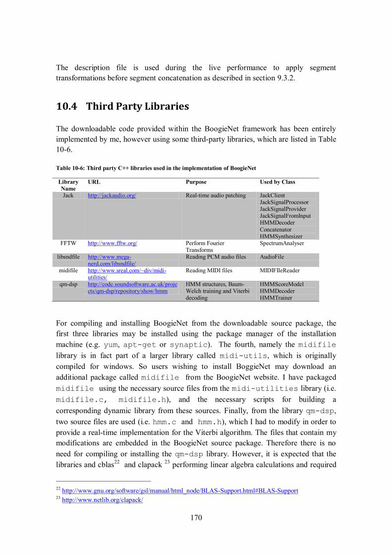
170
The description file is used during the live performance to apply segment
transformations before segment concatenation as described in section 9.3.2.
10.4 Third Party Libraries
The downloadable code provided within the BoogieNet framework has been entirely
implemented by me, however using some third-party libraries, which are listed in Table
10-6.
Table 10-6: Third party C++ libraries used in the implementation of BoogieNet
Library
Name
URL Purpose Used by Class
Jack http://jackaudio.org/ Real-time audio patching JackClient JackSignalProcessor JackSignalProvider JackSignalFromInput HMMDecoder
Concatenator HMMSynthesizer
FFTW http://www.fftw.org/ Perform Fourier Transforms
SpectrumAnalyser
libsndfile http://www.mega-nerd.com/libsndfile/
Reading PCM audio files AudioFile
midifile
http://www.sreal.com/~div/midi-utilities/
Reading MIDI files MIDIFIleReader
qm-dsp http://code.soundsoftware.ac.uk/projects/qm-dsp/repository/show/hmm
HMM structures, Baum-Welch training and Viterbi decoding
HMMScoreModel HMMDecoder HMMTrainer
For compiling and installing BoogieNet from the downloadable source package, the
first three libraries may be installed using the package manager of the installation
machine (e.g. yum, apt-get or synaptic). The fourth, namely the midifile
library is in fact part of a larger library called midi-utils, which is originally
compiled for windows. So users wishing to install BoggieNet may download an
additional package called midifile from the BoogieNet website. I have packaged
midifile using the necessary source files from the midi-utilities library (i.e.
midifile.c, midifile.h), and the necessary scripts for building a
corresponding dynamic library from these sources. Finally, from the library qm-dsp,
two source files are used (i.e. hmm.c and hmm.h), which I had to modify in order to
provide a real-time implementation for the Viterbi algorithm. The files that contain my
modifications are embedded in the BoogieNet source package. Therefore there is no
need for compiling or installing the qm-dsp library. However, it is expected that the
libraries and cblas22
and clapack 23
performing linear algebra calculations and required
22 http://www.gnu.org/software/gsl/manual/html_node/BLAS-Support.html#BLAS-Support 23 http://www.netlib.org/clapack/

171
by the HMM part of the qm-dsp library have been previously installed on the target
machine, which can be done using the available package manager.
Table 10-7: Library dependencies of the BoogieNet framework
[root@mosquito ~]# ldd /usr/local/lib/libboogienet.so
linux-gate.so.1 => (0x0070e000)
libjack.so.0 => /usr/local/lib/libjack.so.0 (0x0018c000)
libsndfile.so.1 => /usr/local/lib/libsndfile.so.1 (0x00afa000)
libmidifile.so.0 => /usr/local/lib/libmidifile.so.0 (0x005c5000)
libgslcblas.so.0 => /usr/lib/libgslcblas.so.0 (0x00a95000)
liblapack.so.3 => /usr/lib/liblapack.so.3 (0x00b53000)
libudp.so.0 => /usr/local/lib/libudp.so.0 (0x00478000)
libstdc++.so.6 => /usr/lib/libstdc++.so.6 (0x001a4000)
libm.so.6 => /lib/libm.so.6 (0x00424000)
libc.so.6 => /lib/libc.so.6 (0x00850000)
libgcc_s.so.1 => /lib/libgcc_s.so.1 (0x00110000)
librt.so.1 => /lib/librt.so.1 (0x00703000)
libpthread.so.0 => /lib/libpthread.so.0 (0x00527000)
libdl.so.2 => /lib/libdl.so.2 (0x0011c000)
libblas.so.3 => /usr/lib/libblas.so.3 (0x00121000)
libgfortran.so.1 => /usr/lib/libgfortran.so.1 (0x0028f000)
/lib/ld-linux.so.2 (0x003b3000)
[root@mosquito ~]# ldd `which boogienet`
linux-gate.so.1 => (0x00ed5000)
libboogienet.so.0 => /usr/local/lib/libboogienet.so.0 (0x00730000)
libjack.so.0 => /usr/local/lib/libjack.so.0 (0x0098b000)
librt.so.1 => /lib/librt.so.1 (0x00901000)
libpthread.so.0 => /lib/libpthread.so.0 (0x00563000)
libdl.so.2 => /lib/libdl.so.2 (0x0055c000)
libsamplerate.so.0 => /usr/lib/libsamplerate.so.0 (0x03254000)
libcelt.so.0 => /usr/lib/libcelt.so.0 (0x0057f000)
libsndfile.so.1 => /usr/local/lib/libsndfile.so.1 (0x00110000)
libmidifile.so.0 => /usr/local/lib/libmidifile.so.0 (0x00431000)
libgslcblas.so.0 => /usr/lib/libgslcblas.so.0 (0x00169000)
liblapack.so.3 => /usr/lib/liblapack.so.3 (0x009a3000)
libudp.so.0 => /usr/local/lib/libudp.so.0 (0x0019b000)
libstdc++.so.6 => /usr/lib/libstdc++.so.6 (0x0019d000)
libm.so.6 => /lib/libm.so.6 (0x00531000)
libgcc_s.so.1 => /lib/libgcc_s.so.1 (0x00288000)
libc.so.6 => /lib/libc.so.6 (0x0058e000)
/lib/ld-linux.so.2 (0x003b3000)
libblas.so.3 => /usr/lib/libblas.so.3 (0x00294000)
libgfortran.so.1 => /usr/lib/libgfortran.so.1 (0x002e7000)
[root@mosquito ~]#
Listing the library dependencies of the boogienet library and the command line
application provides the output shown on Table 10-7.
172
11 Experimental Evaluation
This chapter presents the evaluation of the BoogieNet framework. Specifically, it
provides the results of a number of evaluation experiments assessing the performance of
the algorithms presented in the previous chapters, as well as an experiment of a
collaborative performance over the network. The evaluation of the algorithmic
performance serves to reveal shortcomings of the current implementation that need to be
addressed in future developments. The network experiment reveals the benefits offered
by the proposed communication scheme compared to direct audio stream exchange,
which is the prevalent means of audio communication in Network Music Performances.
The chapter initially discusses some concerns related to the evaluation methodology
which is unavoidably constrained in many respects. Then, the results of the evaluation
of algorithmic performance are presented. The section that follows presents the network
experiment. Finally, the last section consolidates the results and discusses the efficacy
of the proposed communication scheme for NMP.
11.1 Considerations on the evaluation methodology
The comprehensiveness of the evaluation methodology presented in this chapter may be
considered debatable due to a number of reasons. Firstly, it was not possible to perform
a formal user evaluation involving human musicians collaborating over computer
networks, due to the robustness of the implemented algorithms being currently
inadequate for the intended scenario. Secondly, it was not possible to draw conclusions
with respect to practical significance of results due to the limited availability of
appropriate musical material to use in experimental validations. Thirdly, due to the
same reason it was not possible to assess the improvement of the HMM algorithm by
using sufficient training datasets. Finally, minor modifications of algorithm parameters
were required in order to effectively cope with the variability of the temporal
characteristics of different music performances. These issues are further elaborated in
the subsections that follow.
11.1.1 The lack of a formal user evaluation
As the system under investigation integrates achievements from different research
domains, different methodologies may be employed to evaluate its performance. A
formal user evaluation requires for conducting NMP experiments involving human
musicians. Such experiments commonly amount to some music ensemble engaged in
collaborative music performance using an NMP software framework (Alexandraki and
Akoumianakis 2010) or some software/hardware setup that artificially simulates
173
network conditions in terms of one or more parameters such as latency, jitter (Chew et
al. 2005; Driessen, Darcie and Pillay 2011; Chafe et al. 2004) or packet loss.
Subsequently to collaborative performance, the evaluation findings are obtained either
from user ratings provided by performers as responses to a number of questions relating
to their ability to synchronize (Buillot 2007), or by analyzing performance data captured
by appropriate MIDI (Chew et al. 2005) or audio (Driessen, Darcie and Pillay 2011)
apparatus facilitated to capture the live performance. Unfortunately, conducting NMP
experiments is highly expensive in terms of costly human resources. In particular, NMP
experiments requires the participation of professional music ensembles (so as to
eliminate biased conclusions owing to musician’s effort to adapt to each other’s
performance), network engineers (in order to resolve firewall issues and activate the
necessary network ports for audio and possibly video communication), as well as sound
engineers (to appropriately setup audio equipment therefore avoiding feedback loops or
unwanted noise consuming network resources).
The approach under investigation does not literary provide a networking solution, as
there are no contributions in terms of networking technologies (e.g. network protocols
or data routing optimisations). Additionally, the current implementation is far from
being a fully functional software application. Unfortunately, the facilitated algorithms
are not yet sufficiently robust to support the intended scenario. Conversely, the
implemented prototype is the result of early investigations on a new musical interaction
paradigm, which may be used to experiment with new musical ideas, for instance by
alternating between transmitting audio streams and onset notifications. Consequently,
conducting a formal user evaluation (i.e. NMP experiments) is neither feasible for the
current status of this work, nor can it provide any useful information for the task at
hand.
For this reason, the main part of this chapter focuses on evaluating the algorithmic
performance of the methodology presented in the previous chapters. For reasons of
consistency, a network experiment has also been conducted. This experiment involves
the collaboration of two musicians, namely a flutist and a violinist, collaborating across
a Local Area Network (LAN). The evaluation of the algorithmic performance reveals
shortcomings of the current implementation, therefore motivating future research and
development efforts, while the network experiment shows the benefits of employing the
proposed communication scheme over conventional audio stream exchange, which is
the prevalent means of communication in NMP.
11.1.2 Standard evaluation metrics and significance of results
For the evaluation of the algorithmic performance, standard MIR evaluation procedures
have been employed. MIREX (Music Information Retrieval Evaluation eXchange) is a
community-based framework which organises annual contests that provide a de facto
standard for evaluating algorithmic performance in a number of MIR tasks. These MIR
174
tasks24
range from ‘genre recognition’ and ‘music similarity and retrieval’ applied on
large music collections, to tasks focusing on specific music pieces and machine
musicianship such as ‘melody extraction’, ‘beat tracking’ or ‘chord detection’. With
respect to the performance of algorithms operating in real-time, the only relevant task in
MIREX is that of ‘score following’.
MIREX annual contests allow making meaningful comparisons for the performance of
different algorithms targeting a specific task. As the algorithms are evaluated on the
same dataset, an estimator for the best algorithmic performance for each task is
provided on an annual basis. For instance, the maximum total precision for the task of
‘Real-time audio to score alignment (aka score following)’ was 67.11% in 2011,
83.01% in 2012 and 86.70% in 2013. Although these rankings are not necessarily
increasing every year for all of the tasks under evaluation, evaluation metrics are
derived by applying the algorithms on the same audio dataset. Unfortunately, the
majority of MIREX datasets are not freely available to researchers due to musical
intellectual property copyright enforcement. As a result, to compare to the annual
rankings in MIR tasks one should submit their algorithm to the MIREX community
(Downie 2008).
An important issue relating to MIREX evaluation procedures is related to whether such
algorithmic rankings correspond to truly significant differences in performance. To
account for this concern, since 2006 MIREX employed significance tests that measure
the global and pair-wise significance of differences in algorithmic rankings (Downie
2008). As the significance tests used by MIREX are inspired by TREC (Text REtrieval
Conference), a community on text retrieval, significance tests have only been applied to
the tasks that have a closer resemblance to text retrieval. For the tasks of ‘Audio Onset
Detection’ and ‘Real-time Audio to Score Alignment’ that are mostly relevant to the
present work, no significance tests have been applied up to 2013.
Furthermore, with respect to the relationship of user satisfaction in an application
targeted by a MIR task and the algorithmic performance of a system in that task,
Urbano et al. (2012) showed that, for the example task of ‘music similarity and
retrieval’, differences in user satisfaction may be so subtle that statistical significance is
not sufficient to prove the superiority of one algorithm over another. In such cases, one
needs to evaluate for practical significance (i.e. on large-scale datasets) in order to truly
prove real-world user satisfaction. Clearly, practical significance is a lot more difficult
in MIR research, as the systems under evaluation need to have access to large
collections of copyrighted material.
11.1.3 Lack of multiple training sequences
Yet a further concern related to the evaluation of algorithmic performance relates to the
fact that, due to the lack of different recordings for the same piece of music, HMM
24 http://www.music-ir.org/mirex/wiki/2013:Main_Page

175
training and HMM decoding was performed on the same audio file. This causes two
problems. Firstly, as elaborated in section 8.3.3.1, for HMMs having a left-right
topology it is essential that multiple sequences are used so as to accurately train the
model. Hence, the performance measures of audio to score alignment are suboptimal
than those obtained when training on multiple performances of the same piece of music,
as for example in the course of a music rehearsal.
Secondly, in classification problems, testing the performance of a trained classifier on
the data used for training is a method known as resubstitution and it is well known that
performance measures estimated in this way are usually overoptimistic (Flexer 2006
and the references therein). Preferably, a method known as K-fold cross-validation is
employed for evaluating trained classifiers. K-fold cross-validation amounts to dividing
the data into K equally-sized parts and using each part as a test set for the classifier
trained with the remaining data. The performance measures are then the average of
performance measures over the K different runs.
Unfortunately, it was not possible to obtain multiple performances of the same piece of
music so as to use multiple training sequences for each model or to perform a K-fold
cross validation test. In the following experiments the HMM is initialised using the
output of the offline segmentation process as described in section 8.4.1. Subsequently,
the performance of real-time audio to score alignment is evaluated prior to training and
after Baum-Welch training. Finally, a pair-wise t-test is performed to evaluate the
significance of performance improvement through the training process.
11.1.4 Algorithm fine tuning
A further aspect relating to the performed evaluation relates to the number of changes
that may be required when algorithms need to analyse different audio streams. It is
widely known that such algorithms require human supervision in order effectively to
cope with variability in the timbral and temporal variations of each music performance.
In the present evaluation of algorithmic performance, a single parameter was adjusted,
namely the value of the minimum Inter-Onset-Interval. This parameter is used by the
offline audio segmentation algorithm as well as by the HMM score following algorithm
to reduce the number of falsely detected onsets. In future implementations, the value of
this parameter may be automatically estimated by employing techniques for tempo
induction.
11.2 Evaluation of algorithmic performance
This section presents the evaluation of the performance of the algorithms presented in
the previous chapters. These algorithms have been applied on a small dataset that I had
to assemble from various publicly available music sources and manually annotate to
provide ground truth data for the location of note onsets. As elaborated in section
176
11.1.2, the results of this evaluation are not comparable to officially evaluated
algorithms. However, they serve to provide some insight with regards to feasibility of
the proposed communication scheme for NMP. More importantly, the results presented
in the following sections reveal weaknesses of the current implementation to be
addressed in future developments. Evaluation metrics are those used by MIREX
evaluations for the tasks of ‘Audio Onset Detection’ and ‘Real-time Audio to Score
Alignment’, supplemented by some measures that are relevant to the intended
application scenario on Networked Music Performance.
11.2.1 Dataset
At present, a substantial number of music datasets are available on the Internet, some of
them free, without any payment fee. Unfortunately, most of these datasets have been
assembled for more generic music information retrieval tasks, such as genre
classification or music similarity. Assembling an appropriate evaluation dataset for the
present system imposes a number of restrictions that are not commonly met in existing
datasets. These restrictions concern the following aspects:
All sound files should correspond to the performance of a single instrument
The instruments should be monophonic, as no chords or polyphony is being
considered at the present implementation
All sound files should be accompanied by a corresponding MIDI file (i.e. a
music score)
The dataset should contain recordings from different types of instruments so as
to provide insight on potential differences in algorithmic performance for
different musical timbres
In order to satisfy the above restrictions, an evaluation dataset was assembled using
some files from publicly available datasets and some of my own recordings. This
dataset comprises 23 music pieces summing to a total of 969 notes and a total duration
of 9.63 minutes, as listed on Table 11-1. All audio files are uncompressed files in WAV
encoding format, having a sample rate of 44.1 kHz, a bit resolution of 16 bits per
sample, and a single audio channel.
The column entitled ‘FILE-ID provides the filename for the audio file and
corresponding MIDI file and additionally depicts the musical instrument that was used
for the solo recording. Ground truth onset annotations were performed manually and
assisted by Sonic Visualizer25
, an open source software program designed to aid audio
file annotation.
The column entitled ‘SRC’ indicates the dataset from which audio and MIDI files were
derived. Specifically, the files having SRC=1 were derived from the TRIOS26
publicly
25 http://www.sonicvisualiser.org/ 26 http://c4dm.eecs.qmul.ac.uk/rdr/handle/123456789/27
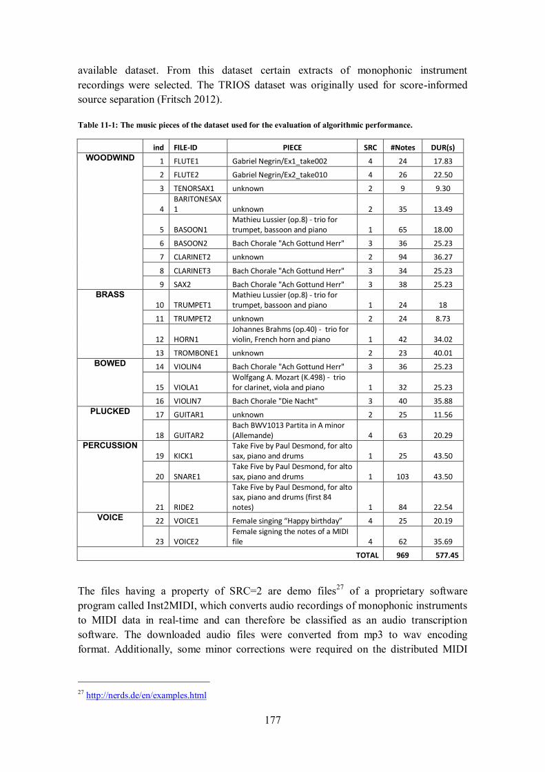
177
available dataset. From this dataset certain extracts of monophonic instrument
recordings were selected. The TRIOS dataset was originally used for score-informed
source separation (Fritsch 2012).
Table 11-1: The music pieces of the dataset used for the evaluation of algorithmic performance.
ind FILE-ID PIECE SRC #Notes DUR(s) WOODWIND 1 FLUTE1 Gabriel Negrin/Ex1_take002 4 24 17.83
2 FLUTE2 Gabriel Negrin/Ex2_take010 4 26 22.50
3 TENORSAX1 unknown 2 9 9.30
4 BARITONESAX1 unknown 2 35 13.49
5 BASOON1 Mathieu Lussier (op.8) - trio for trumpet, bassoon and piano 1 65 18.00
6 BASOON2 Bach Chorale "Ach Gottund Herr" 3 36 25.23
7 CLARINET2 unknown 2 94 36.27
8 CLARINET3 Bach Chorale "Ach Gottund Herr" 3 34 25.23
9 SAX2 Bach Chorale "Ach Gottund Herr" 3 38 25.23 BRASS
10 TRUMPET1 Mathieu Lussier (op.8) - trio for trumpet, bassoon and piano 1 24 18
11 TRUMPET2 unknown 2 24 8.73
12 HORN1 Johannes Brahms (op.40) - trio for violin, French horn and piano 1 42 34.02
13 TROMBONE1 unknown 2 23 40.01 BOWED 14 VIOLIN4 Bach Chorale "Ach Gottund Herr" 3 36 25.23
15 VIOLA1 Wolfgang A. Mozart (K.498) - trio for clarinet, viola and piano 1 32 25.23
16 VIOLIN7 Bach Chorale "Die Nacht" 3 40 35.88 PLUCKED 17 GUITAR1 unknown 2 25 11.56
18 GUITAR2 Bach BWV1013 Partita in A minor (Allemande) 4 63 20.29
PERCUSSION
19 KICK1 Take Five by Paul Desmond, for alto sax, piano and drums 1 25 43.50
20 SNARE1 Take Five by Paul Desmond, for alto sax, piano and drums 1 103 43.50
21 RIDE2
Take Five by Paul Desmond, for alto sax, piano and drums (first 84 notes) 1 84 22.54
VOICE 22 VOICE1 Female singing “Happy birthday” 4 25 20.19
23 VOICE2 Female signing the notes of a MIDI file 4 62 35.69
TOTAL 969 577.45
The files having a property of SRC=2 are demo files27
of a proprietary software
program called Inst2MIDI, which converts audio recordings of monophonic instruments
to MIDI data in real-time and can therefore be classified as an audio transcription
software. The downloaded audio files were converted from mp3 to wav encoding
format. Additionally, some minor corrections were required on the distributed MIDI
27 http://nerds.de/en/examples.html
178
files, which were generated by the Inst2MIDI software and had some minor
imperfections.
The files having a property of SRC=3 have been derived from the Bach10 dataset28
,
which contains audio recordings for ten Bach Chorales for which the four voices
(Soprano, Alto, Tenor and Bass) of each piece are performed by the instruments violin,
clarinet, saxophone and bassoon, respectively. The Bach10 dataset has been assembled
for the purposes of multi-pitch estimation and tracking (Duan, Pardo and Zhang 2010)
as well as for the purposes of score informed audio source separation (Duan and Pardo
2011). The MIDI files of this dataset comprise four channels that correspond to the four
voices of the chorale. Hence, to use them in the present evaluation, different channels
had to be saved in separate MIDI files.
Finally, the files having a property of SRC=4 were recorded for the purposes of the
present evaluation.
With respect to timbral specificities, the following instrument classes were used in the
evaluation dataset:
Woodwind: 8 woodwind solo performances comprising 361 notes in total
Brass: 4 solo performances comprising 113 notes in total
Bowed String: 3 solo performances comprising 108 notes in total
Plucked String: 2 guitar solo comprising 88 notes in total
Percussive: 3 instrument performances comprising 212 notes in total
Vocal: 2 pieces comprising 87 notes in total
11.2.2 Measures
The measures that were used to evaluate the present system are based on the evaluation
measures used by the yearly annual MIREX contests for the tasks of ‘Audio Onset
Detection’29
and ‘Real-time Audio to Score Alignment (a.k.a. Score Following)’30
with
minor changes that are relevant to the intended scenario for networked musical
interactions. Specifically, MIREX uses the following measures to compare the detected
onsets with ground-truth ones:
Ocd: Number of correctly detected onsets (CD). For a given ground-truth onset
time, if there is a detection in a tolerance time-window around it, it is considered
as a correct detection. This tolerance time-window conventionally spans a range
of ±50ms around the ground-truth onset. It is generally not possible to evaluate
on more accurate timing tolerance due to weak precision in ground truth
annotations.
28 http://music.cs.northwestern.edu/data/Bach10.html 29 http://www.music-ir.org/mirex/wiki/2013:Audio_Onset_Detection 30 http://www.music-ir.org/mirex/wiki/2013:Real-time_Audio_to_Score_Alignment_(a.k.a_Score_Following)
179
Ofn: Number of False Negatives (FN). This is the number of ground-truth
onsets that were not detected. In other words, it is the number of ground-truth
onsets for which no onset was detected within a time window ±50ms around
them.
Ofp: Number of False Positives (FP). The number of detections that fall outside
all tolerance windows, namely the number of spurious detections.
MIREX additionally uses the measures of ‘doubled onsets’ (two detections for one
ground-truth onset) and merged onsets (a single detection for two ground-truth onsets).
Doubled onsets are a subset of the FP onsets, and merged onsets a subset of FN onsets.
These measures were not used in the present evaluation because all algorithms impose a
minimum Inter-Onset-Interval criterion of permitting detections only if they are
separated by a predefined threshold value (which was 50ms or higher), therefore
execution of the algorithms did not yield any doubled or merged detections.
The above numbers are used to calculate the F-measure (F), which is a common metric
of algorithm performance in information retrieval and pattern recognition tasks. The F-
measure is computed here as the harmonic mean of Precision (P) and Recall (R)
measures:
, where
and
(11.1)
In the case of score following, two additional metrics have been computed to allow
comparing with the annual reporting of MIREX results in the task of score following.
These are the piecewise precision rate, which is the percentage of ground truth onsets
minus the number of missed onsets of each piece, averaged for all pieces in the dataset,
as well as the overall precision rate, which is the percentage of the total number of
ground truth notes in the dataset minus the total number of missed notes during the
evaluation.
The following values were also computed to provide metrics related to the time
precision of correct onset detections:
Avg. Abs. Offset: The average of the absolute value of the time difference
between a correctly detected onset and the corresponding ground truth onset.
This is always a value below 50ms. The average is calculated for all correct
detections within a specific audio file.
Mean Offset: The mean value of the time difference between a correct detection
and the corresponding ground truth onset. This quantity can have negative
values hence indicating detected onsets may precede the corresponding ground-
truth onsets. The mean is calculated for the total of correct detections within a
certain audio file.
Std Offset: The standard deviation of the timing offset. It gives an idea for the
variability of offset values. Like the mean value the standard deviation is
computed for the total of correct detections within a piece of music.
180
Finally, for the purposes of measuring algorithm speed and related complexity three
measures have been recorded. The first one provides a metric for the speed of the offline
audio segmentation process, the second provides a metric for the speed of real-time
audio to score alignment (also used by MIREX score following evaluations), while the
third one provides a metric for the speed of real-time audio analysis and segmental re-
synthesis in the current system:
Time Elapsed: This provides a speed measurement of the task of offline audio
segmentation, which comprises both onset detection and saving the segments in
different audio files on disk space. Hence, more notes in a music piece are
generally expected to yield higher values of this quantity.
Avg. Latency 1: The latency of the score follower, i.e. difference between
detection time and the time when the system captures an audio block. This
measurement is recorded at onset detections and averaged for all detected onsets
within the audio file.
Avg. Latency 2: This is the time elapsed between the arrival of a new audio
block and the rendering of a transformed audio segment recorded at every onset
detection and averaged for all detected onsets. In other words this refers to the
total latency that may be decomposed to latency for the detection of the new
onset (i.e. Avg. Latency 1) and the latency introduced by segmental re-synthesis
during the live performance. This measure is intended for comparison with the
Ensemble Performance Threshold (see section 2.4), as it incorporates all
processing latencies apart from network transmission. The latency of re-
synthesis alone is thus equal to the difference Avg_Latency_2 – Avg_Latency_1
11.2.3 Experimental setup
All of the experiments were performed on the same computer, a Lenovo Thinkpad with
an Intel Core Duo 2GHz processor, 2GB RAM and a CentOS5 Linux distribution.
Three processes were executed to assess the performance of the algorithms under
evaluation:
OAS: Offline Audio Segmentation, i.e. by issuing the following command line
process:
o boogienet –p oas –a FLUTE1.wav –s FLUTE1.mid –d /tmp
RTAS-INIT: Real-time Audio to Score Alignment based on an HMM, which is
initialised according to annotations based on the note onsets detected during
offline audio segmentation and a number of heuristics (see section 8.4.1). The
evaluation of this process involved issuing the following commands:
o boogienet –p oas –a FLUTE1.wav –s FLUTE1.mid –d /tmp
o boogienet –p pma –a FLUTE1.wav –s FLUTE1.mid –m
FLUTE1.model
181
o boogienet –p rtas –m FLUTE1.model –d /tmp –t –n
FLUTE1.wav.desc
RTAS-TRAINED: Real-time Audio to Score Alignment based on a
performance model initialised as previously and subsequently trained to obtain
more accurate estimations of HMM probabilities. The evaluation of this process
involved issuing the following commands:
o boogienet –p oas –a FLUTE1.wav –s FLUTE1.mid –d /tmp
o boogienet –p pma –a FLUTE1.wav –s FLUTE1.mid –m
FLUTE1.model
o boogienet –p tpm –m FLUTE1.model –a FLUTE1.wav
o boogienet –p rtas –m FLUTE1.model –d /tmp –t –n
FLUTE1.wav.desc
In the above, the command line process invocation is shown for an example audio/MIDI
file pair ‘FLUTE1.wav’ and ‘FLUTE1.mid’. Real-time audio capturing and playback
was appropriately routed to the BoogieNet application using the Jack Audio Connection
Kit, as explained in section 10.2.5. This process does not involve any network
transmissions. The –n flag for the processes RTAS-INIT and RTAS-TRAINED
indicates that segment transformations were activated during segmental re-synthesis.
Each of these processes was setup to print on standard output the location of the
detected onsets as well as the speed of the algorithms (i.e. ‘Time Elapsed’ for the OAS
process and ‘Latency 1’, ‘Latency 2’ for every onset detected by the processes RTAS-
INIT and RTAS-TRAINED). Subsequently, to the execution of these programs a utility
program (implemented for this purpose) was executed to automatically compute the
remaining evaluation metrics (e.g. correct detections, false positives, F-Measure,
averages of timing offsets etc.).
11.2.4 Offline Audio Segmentation (OAS)
The detailed (i.e. piecewise) results of the offline audio segmentation process are shown
on Table 13-1 of the Appendix. A summary of these results is provided on Table 11-2,
which shows the most important measures estimated for all pieces within an instrument
class. The column %TP refers to the percentage of true positives, while %FP refers to
the percentage of false positives summed for the total of number of onsets appearing in
all pieces of music within the instrument class. The column ‘Avg. F’ refers to the value
of the F-measure per piece, which is averaged for all the pieces of an instrument class.
F-measure averages are also depicted in Figure 11-1. While %TP refers to the global
percentage of correct detections, ‘Avg. F’ refers to the average of correct detections as
estimated by equations (11.1). Also, the averages appearing at the bottom row of Table
11-2 are class averages, while the bottom row of Table 13-1 refers to piecewise
averages.
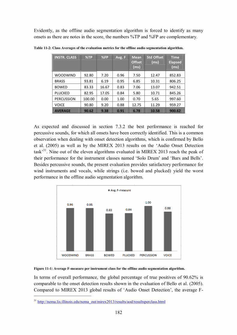
182
Evidently, as the offline audio segmentation algorithm is forced to identify as many
onsets as there are notes in the score, the numbers %TP and %FP are complementary.
Table 11-2: Class Averages of the evaluation metrics for the offline audio segmentation algorithm.
INSTR. CLASS %TP %FP Avg. F Mean Offset (ms)
Std Offset (ms)
Time Elapsed
(ms)
WOODWIND 92.80 7.20 0.96 7.50 12.47 852.83
BRASS 93.81 6.19 0.95 6.85 10.31 806.25
BOWED 83.33 16.67 0.83 7.06 13.07 942.51
PLUCKED 82.95 17.05 0.84 5.80 10.71 845.26
PERCUSSION 100.00 0.00 1.00 0.70 5.65 997.60
VOICE 90.80 9.20 0.88 12.75 11.29 959.27
AVERAGE 90.62 9.38 0.91 6.78 10.58 900.62
As expected and discussed in section 7.3.2 the best performance is reached for
percussive sounds, for which all onsets have been correctly identified. This is a common
observation when dealing with onset detection algorithms, which is confirmed by Bello
et al. (2005) as well as by the MIREX 2013 results on the ‘Audio Onset Detection
task’31
. Nine out of the eleven algorithms evaluated in MIREX 2013 reach the peak of
their performance for the instrument classes named ‘Solo Drum’ and ‘Bars and Bells’.
Besides percussive sounds, the present evaluation provides satisfactory performance for
wind instruments and vocals, while strings (i.e. bowed and plucked) yield the worst
performance in the offline audio segmentation algorithm.
Figure 11-1: Average F-measure per instrument class for the offline audio segmentation algorithm.
In terms of overall performance, the global percentage of true positives of 90.62% is
comparable to the onset detection results shown in the evaluation of Bello et al. (2005).
Compared to MIREX 2013 global results of ‘Audio Onset Detection’, the average F-
31 http://nema.lis.illinois.edu/nema_out/mirex2013/results/aod/resultsperclass.html

183
measure is higher than all the eleven algorithms evaluated32
. Clearly, this does not mean
that the algorithm evaluated here is superior to the algorithms evaluated by MIREX,
since a significant amount of performance degradation should be expected when
evaluating on larger datasets.
With respect to the timing precision of the detected onsets, Figure 11-2 shows the mean
and standard deviation values of the offset between the time of correct onset detections
and that of the corresponding ground truth annotation, computed for all pieces
belonging to an instrument class. It can be seen that the offset does not increase beyond
25ms compared to the ground truth onset, while again percussive instruments have the
smallest timing offset and the smallest variance. Evaluations of onset detection
algorithms reported elsewhere do not provide results for this measure, as due to weak
precision of the ground truth annotation process, timing offsets considered rather
unimportant. However, it is worth noticing here that bowed instruments exhibit the
largest variation while percussive instruments exhibit the shortest variation.
Figure 11-2: Mean and standard deviation values for the timing offset of the detected onsets for the of offline
audio segmentation algorithm.
Finally in terms of speed, the algorithm runs in less than two seconds in all the cases
evaluated, i.e. with the number of notes per piece ranging between 9 and 103. As
confirmed by Table 13-1, the number of notes to be found increases the execution time,
which can go up to 1.5sec for the 103 notes of the snare drum (SNARE1). This time
interval includes onset detections as well as reading the audio and MIDI file and writing
audio segments on disk space.
32 http://nema.lis.illinois.edu/nema_out/mirex2013/results/aod/summary.html
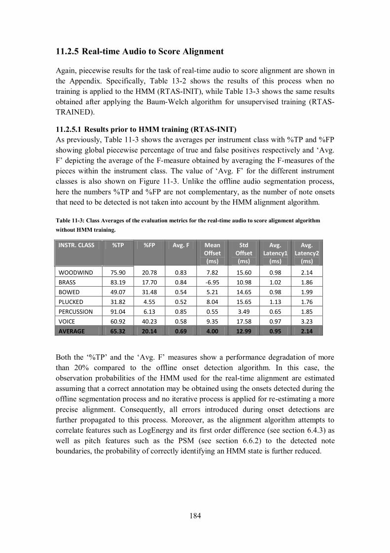
184
11.2.5 Real-time Audio to Score Alignment
Again, piecewise results for the task of real-time audio to score alignment are shown in
the Appendix. Specifically, Table 13-2 shows the results of this process when no
training is applied to the HMM (RTAS-INIT), while Table 13-3 shows the same results
obtained after applying the Baum-Welch algorithm for unsupervised training (RTAS-
TRAINED).
11.2.5.1 Results prior to HMM training (RTAS-INIT)
As previously, Table 11-3 shows the averages per instrument class with %TP and %FP
showing global piecewise percentage of true and false positives respectively and ‘Avg.
F’ depicting the average of the F-measure obtained by averaging the F-measures of the
pieces within the instrument class. The value of ‘Avg. F’ for the different instrument
classes is also shown on Figure 11-3. Unlike the offline audio segmentation process,
here the numbers %TP and %FP are not complementary, as the number of note onsets
that need to be detected is not taken into account by the HMM alignment algorithm.
Table 11-3: Class Averages of the evaluation metrics for the real-time audio to score alignment algorithm
without HMM training.
INSTR. CLASS %TP %FP Avg. F Mean Offset (ms)
Std Offset (ms)
Avg. Latency1
(ms)
Avg. Latency2
(ms)
WOODWIND 75.90 20.78 0.83 7.82 15.60 0.98 2.14
BRASS 83.19 17.70 0.84 -6.95 10.98 1.02 1.86
BOWED 49.07 31.48 0.54 5.21 14.65 0.98 1.99
PLUCKED 31.82 4.55 0.52 8.04 15.65 1.13 1.76
PERCUSSION 91.04 6.13 0.85 0.55 3.49 0.65 1.85
VOICE 60.92 40.23 0.58 9.35 17.58 0.97 3.23
AVERAGE 65.32 20.14 0.69 4.00 12.99 0.95 2.14
Both the ‘%TP’ and the ‘Avg. F’ measures show a performance degradation of more
than 20% compared to the offline onset detection algorithm. In this case, the
observation probabilities of the HMM used for the real-time alignment are estimated
assuming that a correct annotation may be obtained using the onsets detected during the
offline segmentation process and no iterative process is applied for re-estimating a more
precise alignment. Consequently, all errors introduced during onset detections are
further propagated to this process. Moreover, as the alignment algorithm attempts to
correlate features such as LogEnergy and its first order difference (see section 6.4.3) as
well as pitch features such as the PSM (see section 6.6.2) to the detected note
boundaries, the probability of correctly identifying an HMM state is further reduced.
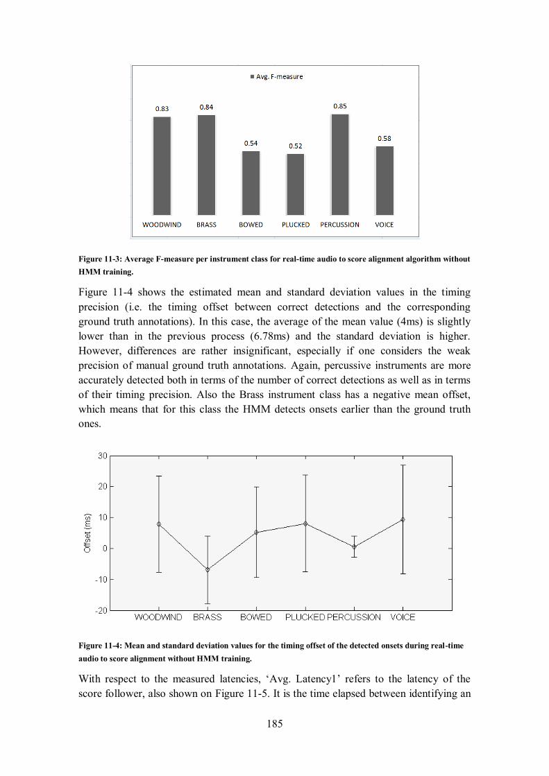
185
Figure 11-3: Average F-measure per instrument class for real-time audio to score alignment algorithm without
HMM training.
Figure 11-4 shows the estimated mean and standard deviation values in the timing
precision (i.e. the timing offset between correct detections and the corresponding
ground truth annotations). In this case, the average of the mean value (4ms) is slightly
lower than in the previous process (6.78ms) and the standard deviation is higher.
However, differences are rather insignificant, especially if one considers the weak
precision of manual ground truth annotations. Again, percussive instruments are more
accurately detected both in terms of the number of correct detections as well as in terms
of their timing precision. Also the Brass instrument class has a negative mean offset,
which means that for this class the HMM detects onsets earlier than the ground truth
ones.
Figure 11-4: Mean and standard deviation values for the timing offset of the detected onsets during real-time
audio to score alignment without HMM training.
With respect to the measured latencies, ‘Avg. Latency1’ refers to the latency of the
score follower, also shown on Figure 11-5. It is the time elapsed between identifying an
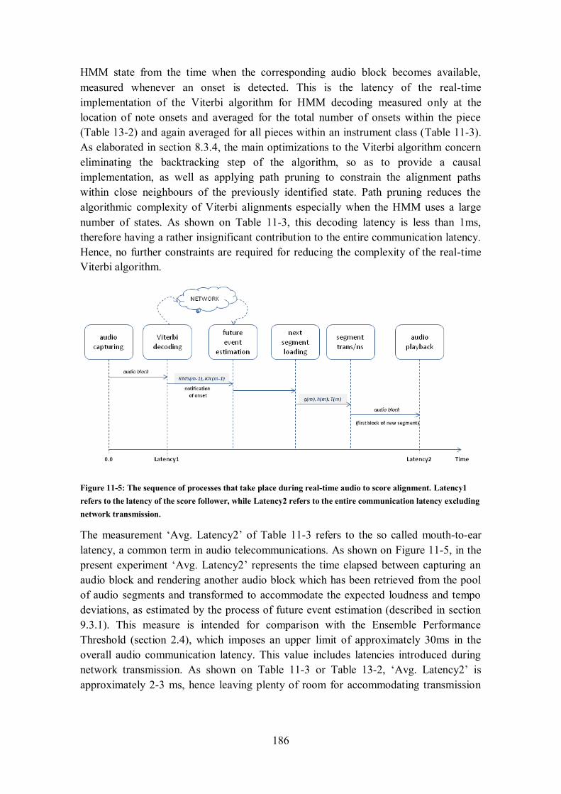
186
HMM state from the time when the corresponding audio block becomes available,
measured whenever an onset is detected. This is the latency of the real-time
implementation of the Viterbi algorithm for HMM decoding measured only at the
location of note onsets and averaged for the total number of onsets within the piece
(Table 13-2) and again averaged for all pieces within an instrument class (Table 11-3).
As elaborated in section 8.3.4, the main optimizations to the Viterbi algorithm concern
eliminating the backtracking step of the algorithm, so as to provide a causal
implementation, as well as applying path pruning to constrain the alignment paths
within close neighbours of the previously identified state. Path pruning reduces the
algorithmic complexity of Viterbi alignments especially when the HMM uses a large
number of states. As shown on Table 11-3, this decoding latency is less than 1ms,
therefore having a rather insignificant contribution to the entire communication latency.
Hence, no further constraints are required for reducing the complexity of the real-time
Viterbi algorithm.
Figure 11-5: The sequence of processes that take place during real-time audio to score alignment. Latency1
refers to the latency of the score follower, while Latency2 refers to the entire communication latency excluding
network transmission.
The measurement ‘Avg. Latency2’ of Table 11-3 refers to the so called mouth-to-ear
latency, a common term in audio telecommunications. As shown on Figure 11-5, in the
present experiment ‘Avg. Latency2’ represents the time elapsed between capturing an
audio block and rendering another audio block which has been retrieved from the pool
of audio segments and transformed to accommodate the expected loudness and tempo
deviations, as estimated by the process of future event estimation (described in section
9.3.1). This measure is intended for comparison with the Ensemble Performance
Threshold (section 2.4), which imposes an upper limit of approximately 30ms in the
overall audio communication latency. This value includes latencies introduced during
network transmission. As shown on Table 11-3 or Table 13-2, ‘Avg. Latency2’ is
approximately 2-3 ms, hence leaving plenty of room for accommodating transmission
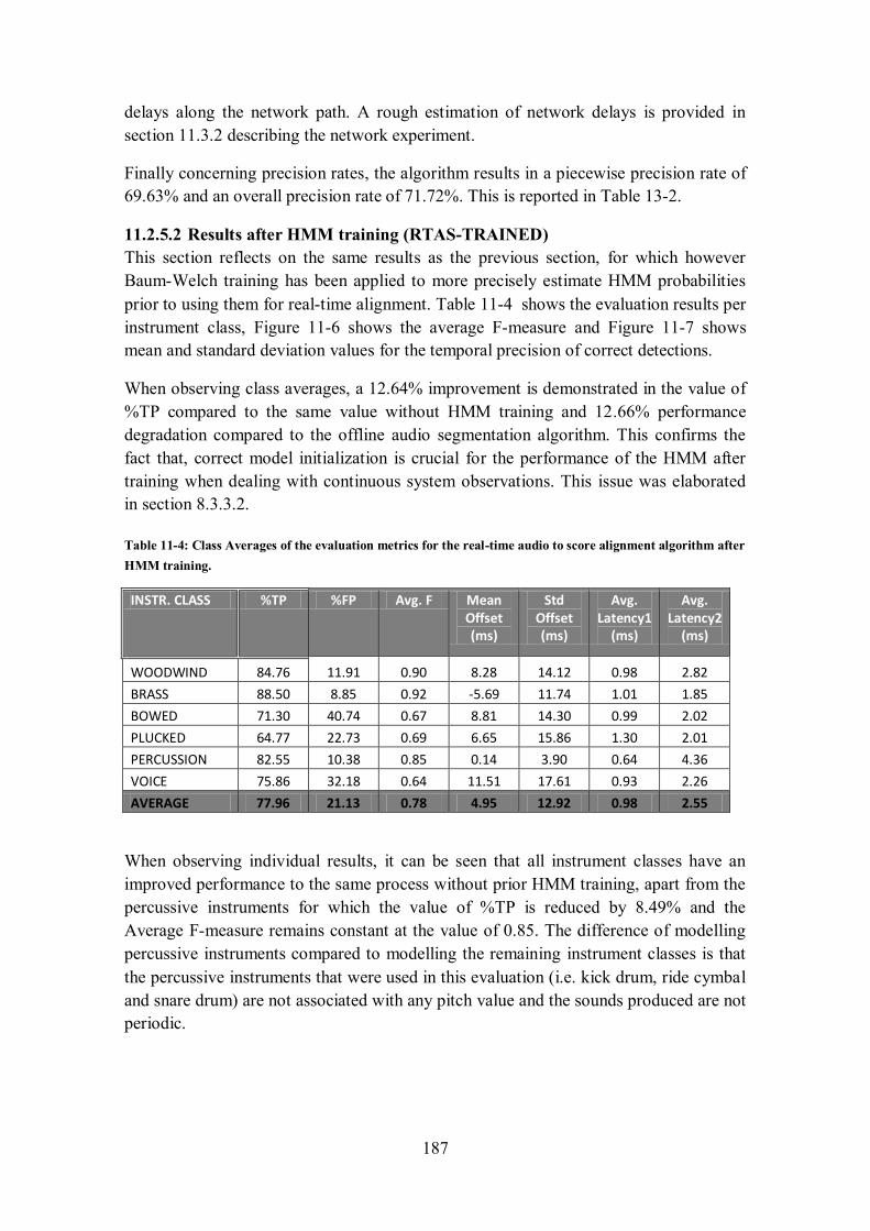
187
delays along the network path. A rough estimation of network delays is provided in
section 11.3.2 describing the network experiment.
Finally concerning precision rates, the algorithm results in a piecewise precision rate of
69.63% and an overall precision rate of 71.72%. This is reported in Table 13-2.
11.2.5.2 Results after HMM training (RTAS-TRAINED)
This section reflects on the same results as the previous section, for which however
Baum-Welch training has been applied to more precisely estimate HMM probabilities
prior to using them for real-time alignment. Table 11-4 shows the evaluation results per
instrument class, Figure 11-6 shows the average F-measure and Figure 11-7 shows
mean and standard deviation values for the temporal precision of correct detections.
When observing class averages, a 12.64% improvement is demonstrated in the value of
%TP compared to the same value without HMM training and 12.66% performance
degradation compared to the offline audio segmentation algorithm. This confirms the
fact that, correct model initialization is crucial for the performance of the HMM after
training when dealing with continuous system observations. This issue was elaborated
in section 8.3.3.2.
Table 11-4: Class Averages of the evaluation metrics for the real-time audio to score alignment algorithm after
HMM training.
INSTR. CLASS %TP %FP Avg. F Mean Offset (ms)
Std Offset (ms)
Avg. Latency1
(ms)
Avg. Latency2
(ms)
WOODWIND 84.76 11.91 0.90 8.28 14.12 0.98 2.82
BRASS 88.50 8.85 0.92 -5.69 11.74 1.01 1.85
BOWED 71.30 40.74 0.67 8.81 14.30 0.99 2.02
PLUCKED 64.77 22.73 0.69 6.65 15.86 1.30 2.01
PERCUSSION 82.55 10.38 0.85 0.14 3.90 0.64 4.36
VOICE 75.86 32.18 0.64 11.51 17.61 0.93 2.26
AVERAGE 77.96 21.13 0.78 4.95 12.92 0.98 2.55
When observing individual results, it can be seen that all instrument classes have an
improved performance to the same process without prior HMM training, apart from the
percussive instruments for which the value of %TP is reduced by 8.49% and the
Average F-measure remains constant at the value of 0.85. The difference of modelling
percussive instruments compared to modelling the remaining instrument classes is that
the percussive instruments that were used in this evaluation (i.e. kick drum, ride cymbal
and snare drum) are not associated with any pitch value and the sounds produced are not
periodic.

188
Figure 11-6: Average F-measure per instrument class for real-time audio to score alignment algorithm after
HMM training.
According to the General MIDI standard, non-chromatic percussion use MIDI Channel
10 and a different pitch value to define the instrument timbre to use when synthesizing
the output sound. The MIDI files used in this case had the note number of 36 for the
kick drum, 59 for the ride cymbal and 38 for the snare drum. Therefore, each piece
evaluated in the percussion class holds a single pitch value, which corresponds to the
instrument rather than the dominating pitch. As a result, the PSM feature and its first
order difference (section 6.6.2) used in the computation of emission probabilities, have
little or no correlation to the actual notes performed in the audio file, which explains the
poor performance of the model in percussive instruments both before as well as after
Baum-Welch training. Conversely, it may be assumed that, as the PSM features are
important for the performance of HMM alignments, the more the pitches used in a
certain piece of music the better the performance of the HMM.
Figure 11-7: Mean and standard deviation values for the timing offset of the detected onsets during real-time
audio to score alignment after HMM training.

189
Other than the improvement in the number of correct onset detections, there are no
significant differences in the temporal precision or in algorithmic latencies.
Finally concerning precision rates, the algorithm yields a piecewise precision rate of
79.14% and an overall precision rate of 80.60%. These values are reported in Table 13-
3. Compared to real-time audio to score alignment without training there is an
approximate improvement of 10% in both rates.
11.2.6 Comparison of Results
The previous sections provided evidence that the performance of the Offline Audio
Segmentation (OAS) process determines the quality of the Real-time Audio to Score
Alignments (RTAS). When the probabilities of the HMM were initialized based on the
onsets detected by the OAS process (RTAS-INIT), the performance of the real-time
HMM alignment was degraded compared to that of the OAS process by approximately
25% in terms of the %TP measure and by 22% in terms of the F-measure (which takes
into account both false positives and false negatives). By applying Baum-Welch
training, subsequently to model initialization and before the alignment (RTAS-
TRAINED), this performance was improved by 12.64% in terms of %TP and 11% in
the F-measure, compared to the alignment performance without training (RTAS-INIT).
Figure 11-8: Box plot depicting the F-measure performance of the three algorithms (OAS, RTAS-INIT and
RTAS-TRAIN) for the task of onset detection. Distributions concern the F-measure values for each music
piece of the evaluation dataset.
This is further verified by the box plot of Figure 11-8 showing the distribution of the
value of F-measure for all music pieces that have been evaluated. It can be seen that
more than 50% of the pieces had an F-measure of more than 0.95 in OAS, 0.74 in
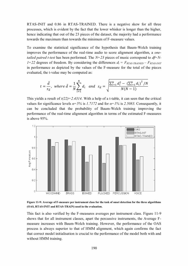
190
RTAS-INIT and 0.86 in RTAS-TRAINED. There is a negative skew for all three
processes, which is evident by the fact that the lower whisker is longer than the higher,
hence indicating that out of the 23 pieces of the dataset, the majority had a performance
towards the maximum than towards the minimum of F-measure values.
To examine the statistical significance of the hypothesis that Baum-Welch training
improves the performance of the real-time audio to score alignment algorithm, a one-
tailed paired t-test has been performed. The N=23 pieces of music correspond to df=N-
1=22 degrees of freedom. By considering the differences di = FRTAS-TRAINED – FRTAS-INIT
in performance as depicted by the values of the F-measure for the total of the pieces
evaluated, the t-value may be computed as:
This yields a result of t(22)=2.4314. With a help of a t-table, it can seen that the critical
values for significance levels α=5% is 1.7172 and for α=1% is 2.5083. Consequently, it
can be concluded that the probability of Baum-Welch training improving the
performance of the real-time alignment algorithm in terms of the estimated F-measures
is above 95%.
Figure 11-9: Average of F-measure per instrument class for the task of onset detection for the three algorithms
(OAS, RTAS-INIT and RTAS-TRAIN) used in the evaluation.
This fact is also verified by the F-measures averages per instrument class. Figure 11-9
shows that for all instrument classes, apart the percussive instruments, the Average F-
measure increases with Baum-Welch training. However, the performance of the OAS
process is always superior to that of HMM alignment, which again confirms the fact
that correct model initialisation is crucial to the performance of the model both with and
without HMM training.
191
Regarding the instruments of the percussion class, the absence of performance
differences before and after training, which can also be seen in Table 13-2 and Table
13-3, is caused by the fact that there is only one pitch value per piece, which does not
even correspond to the dominating pitch of the notes. As discussed in the previous
section, sounds of percussive instruments do not correspond to periodic waveforms, and
therefore the use of PSM features in the computation of the emission probabilities is
misleading for the performance of the model both before and after Baum-Welch
training. An alternative model, relying solely on timbral features needs to be employed
for more accurate score following of non-chromatic percussion instruments.
11.2.7 On the performance of segmental re-synthesis
The research methodology employed for the development of the BoogieNet framework
comprises three computational processes: offline audio segmentation (described in
chapter 7 and evaluated in section 11.2.4), HMM score following (described in chapter
8 and evaluated in section 11.2.5) and segmental re-synthesis (described in chapter 9).
An evaluation of the algorithmic performance of segmental re-synthesis has not been
performed.
The segmental re-synthesis technique that was devised for the system under
investigation has been optimized for speed and algorithmic complexity, but the quality
of the synthesized audio is heavily dependent on the algorithmic performance of the
offline audio segmentation and the score following algorithms.
Duration transformations are applied pitch synchronously assuming that each audio
segment is highly periodic having the period specified in the performance description
file (section 10.3.2.3). As a result, if the offline segmentation process misses an onset
(i.e. false negative detection) then the segment being transformed will contain two
notes, which most likely will have different pitch. Applying duration transformations on
that segment will assume the pitch of the first note to be valid over two notes, hence
resulting in audible distortion during the second note owing to signal discontinuities.
Conversely, if the offline audio segmentation process yields a false positive (i.e. a
spurious detection), then the corresponding audio segment will contain part of that note
and the subsequent segment will contain the remaining part of that note and possibly the
next note. Time scaling the second segment will be performed using the pitch of the
second note for the entire duration of the segment, again resulting in audible signal
distortions.
If the offline segmentation process does not provide any wrong detections (i.e. missed
or spurious onsets), then errors in the score following process do not necessarily result
in audible distortion. For example, missing an onset of the live performance will result
in the previous note being rendered longer than needed, while detecting a false positive
on the live performance will result in the next note being rendered remotely while the
192
previous note still holds. Of course, this assumes that note durations are precisely
estimated.
As was described in section 9.3.1, the estimated note duration at the time of real-time
onset detections is not very precise and it is based on averaging tempo deviations for the
previous notes. This clearly does not reflect true tempo deviations and in the event of a
note of the live performance holding longer than estimated, silence will be appended to
the concatenated note segment. This introduces an additional disturbance in the case of
live performance.
Clearly, the segmental re-synthesis algorithm needs several improvements. Techniques
for instant tempo estimation need to be employed in order to more precisely estimate
the expected tempo deviations of the live performance compared to the pre-existing
recording. Moreover, the evaluation showed that the offline segmentation process needs
to be further improved for robustness, or a synthesis technique based on the phase
vocoder needs to be incorporated in order to eliminate the distortion caused by errors
during the offline audio segmentation algorithm.
11.3 Network experiment
The evaluation of algorithmic performance demonstrated that although the algorithms
implemented in this work do not yield sub-optimal performance to alternative
algorithms for the MIR tasks of onset detection and score following, they are inefficient
for unconditionally supporting the intended communication scheme during NMP. The
algorithms need further improvements in terms of correctly identifying note onsets both
in offline and in real-time contexts and in certain cases, for example the synthesis
algorithm, need to be re-designed in order to more effectively cope with variations in
musical performance. However, as the proposed communication scheme offers
significant benefits compared to conventional raw or encoded audio stream exchange,
this section presents a basic networked experiment that provides insight to the expected
network traffic in an ideal (with respect to algorithmic performance) scenario of
segmental machine listening and re-synthesis over the network.
The experiment involves two music performers, a flutist and a violinist, performing the
same piece of music over the Ethernet. The score of the music piece is depicted on
Figure 11-10. It can be seen that the performance of the flute is associated with 24
onsets, while the performance of the violin has 22 onsets (i.e. 23 notes including ties).
This piece was composed for the purposes of this experiment.
The “Real-time UDP Communication” functionality of the BoogieNet framework
(section 10.2.6) was used for the communication between performers. Network traffic
was captured using Wireshark33
, which is a free, open source and cross platform
33 http://www.wireshark.org
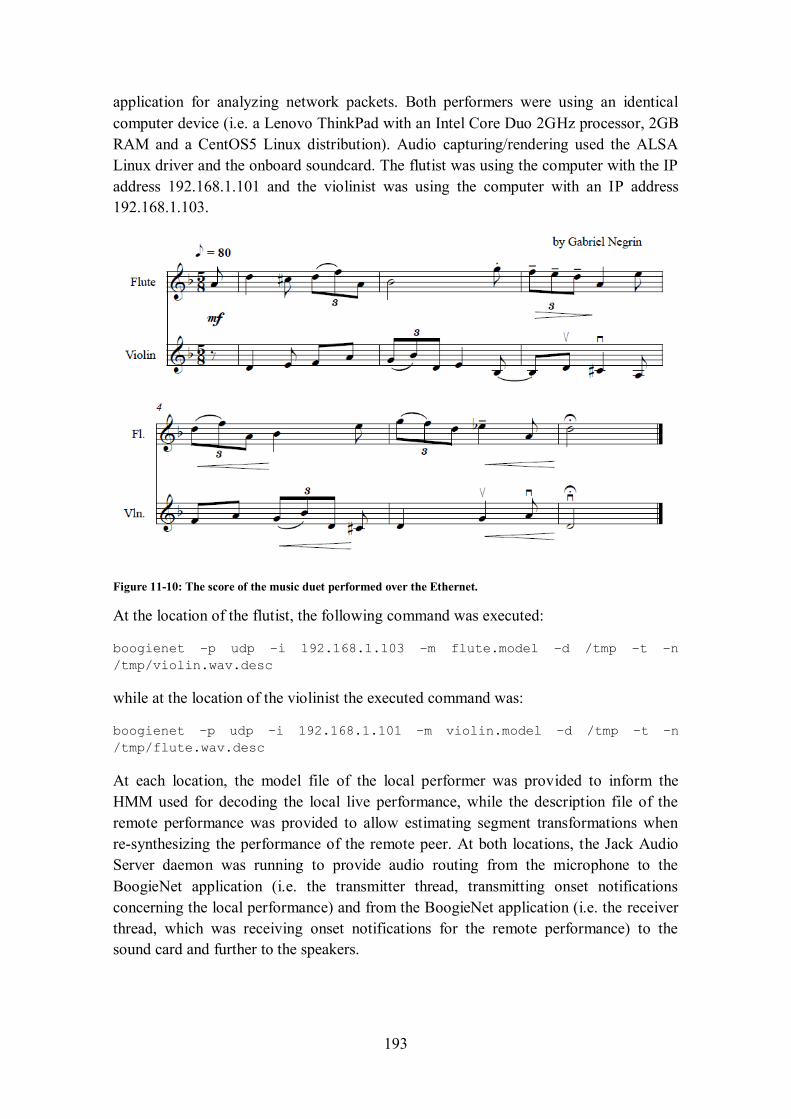
193
application for analyzing network packets. Both performers were using an identical
computer device (i.e. a Lenovo ThinkPad with an Intel Core Duo 2GHz processor, 2GB
RAM and a CentOS5 Linux distribution). Audio capturing/rendering used the ALSA
Linux driver and the onboard soundcard. The flutist was using the computer with the IP
address 192.168.1.101 and the violinist was using the computer with an IP address
192.168.1.103.
Figure 11-10: The score of the music duet performed over the Ethernet.
At the location of the flutist, the following command was executed:
boogienet –p udp –i 192.168.1.103 –m flute.model –d /tmp –t –n
/tmp/violin.wav.desc
while at the location of the violinist the executed command was:
boogienet –p udp –i 192.168.1.101 –m violin.model –d /tmp –t –n
/tmp/flute.wav.desc
At each location, the model file of the local performer was provided to inform the
HMM used for decoding the local live performance, while the description file of the
remote performance was provided to allow estimating segment transformations when
re-synthesizing the performance of the remote peer. At both locations, the Jack Audio
Server daemon was running to provide audio routing from the microphone to the
BoogieNet application (i.e. the transmitter thread, transmitting onset notifications
concerning the local performance) and from the BoogieNet application (i.e. the receiver
thread, which was receiving onset notifications for the remote performance) to the
sound card and further to the speakers.
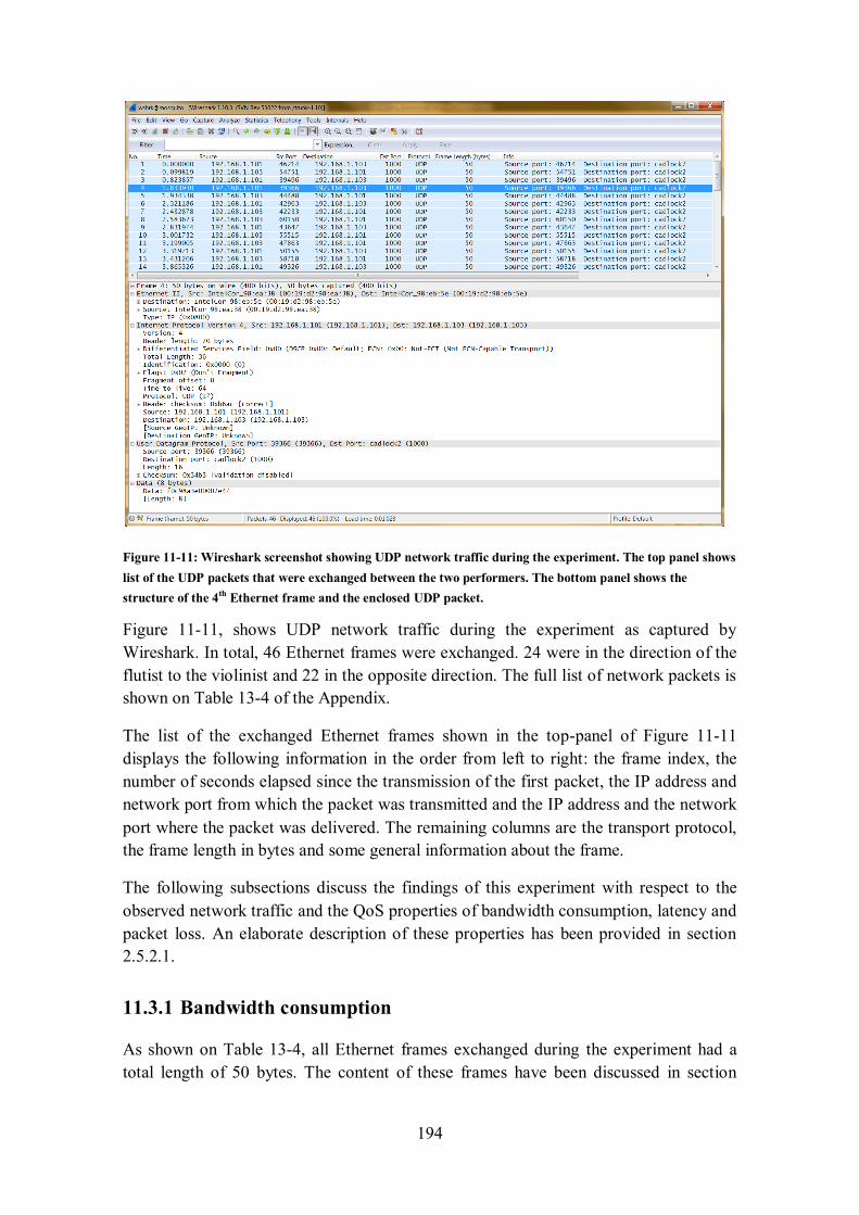
194
Figure 11-11: Wireshark screenshot showing UDP network traffic during the experiment. The top panel shows
list of the UDP packets that were exchanged between the two performers. The bottom panel shows the
structure of the 4th
Ethernet frame and the enclosed UDP packet.
Figure 11-11, shows UDP network traffic during the experiment as captured by
Wireshark. In total, 46 Ethernet frames were exchanged. 24 were in the direction of the
flutist to the violinist and 22 in the opposite direction. The full list of network packets is
shown on Table 13-4 of the Appendix.
The list of the exchanged Ethernet frames shown in the top-panel of Figure 11-11
displays the following information in the order from left to right: the frame index, the
number of seconds elapsed since the transmission of the first packet, the IP address and
network port from which the packet was transmitted and the IP address and the network
port where the packet was delivered. The remaining columns are the transport protocol,
the frame length in bytes and some general information about the frame.
The following subsections discuss the findings of this experiment with respect to the
observed network traffic and the QoS properties of bandwidth consumption, latency and
packet loss. An elaborate description of these properties has been provided in section
2.5.2.1.
11.3.1 Bandwidth consumption
As shown on Table 13-4, all Ethernet frames exchanged during the experiment had a
total length of 50 bytes. The content of these frames have been discussed in section
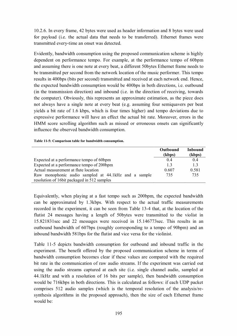
195
10.2.6. In every frame, 42 bytes were used as header information and 8 bytes were used
for payload (i.e. the actual data that needs to be transferred). Ethernet frames were
transmitted every-time an onset was detected.
Evidently, bandwidth consumption using the proposed communication scheme is highly
dependent on performance tempo. For example, at the performance tempo of 60bpm
and assuming there is one note at every beat, a different 50bytes Ethernet frame needs to
be transmitted per second from the network location of the music performer. This tempo
results in 400bps (bits per second) transmitted and received at each network end. Hence,
the expected bandwidth consumption would be 400bps in both directions, i.e. outbound
(in the transmission direction) and inbound (i.e. in the direction of receiving, towards
the computer). Obviously, this represents an approximate estimation, as the piece does
not always have a single note at every beat (e.g. assuming four semiquavers per beat
yields a bit rate of 1.6 kbps, which is four times higher) and tempo deviations due to
expressive performance will have an effect the actual bit rate. Moreover, errors in the
HMM score scrolling algorithm such as missed or erroneous onsets can significantly
influence the observed bandwidth consumption.
Table 11-5: Comparison table for bandwidth consumption.
Outbound
(kbps)
Inbound
(kbps)
Expected at a performance tempo of 60bpm 0.4 0.4
Expected at a performance tempo of 200bpm 1.3 1.3
Actual measurement at flute location 0.607 0.581 Raw monophonic audio sampled at 44.1kHz and a sample
resolution of 16bit packaged in 512 samples
735 735
Equivalently, when playing at a fast tempo such as 200bpm, the expected bandwidth
can be approximated by 1.3kbps. With respect to the actual traffic measurements
recorded in the experiment, it can be seen from Table 13-4 that, at the location of the
flutist 24 messages having a length of 50bytes were transmitted to the violist in
15.821831sec and 22 messages were received in 15.146773sec. This results in an
outbound bandwidth of 607bps (roughly corresponding to a tempo of 90bpm) and an
inbound bandwidth 581bps for the flutist and vice versa for the violinist.
Table 11-5 depicts bandwidth consumption for outbound and inbound traffic in the
experiment. The benefit offered by the proposed communication scheme in terms of
bandwidth consumption becomes clear if these values are compared with the required
bit rate in the communication of raw audio streams. If the experiment was carried out
using the audio streams captured at each site (i.e. single channel audio, sampled at
44.1kHz and with a resolution of 16 bits per sample), then bandwidth consumption
would be 716kbps in both directions. This is calculated as follows: if each UDP packet
comprises 512 audio samples (which is the temporal resolution of the analysis/re-
synthesis algorithms in the proposed approach), then the size of each Ethernet frame
would be:
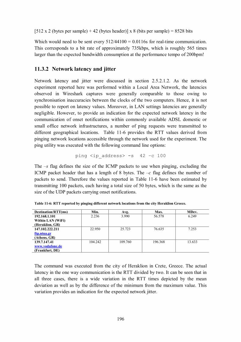
196
[512 x 2 (bytes per sample) + 42 (bytes header)] x 8 (bits per sample) = 8528 bits
Which would need to be sent every 512/44100 = 0.0116s for real-time communication.
This corresponds to a bit rate of approximately 735kbps, which is roughly 565 times
larger than the expected bandwidth consumption at the performance tempo of 200bpm!
11.3.2 Network latency and jitter
Network latency and jitter were discussed in section 2.5.2.1.2. As the network
experiment reported here was performed within a Local Area Network, the latencies
observed in Wireshark captures were generally comparable to those owing to
synchronisation inaccuracies between the clocks of the two computers. Hence, it is not
possible to report on latency values. Moreover, in LAN settings latencies are generally
negligible. However, to provide an indication for the expected network latency in the
communication of onset notifications within commonly available ADSL domestic or
small office network infrastructures, a number of ping requests were transmitted to
different geographical locations. Table 11-6 provides the RTT values derived from
pinging network locations accessible through the network used for the experiment. The
ping utility was executed with the following command line options:
ping <ip_address> -s 42 –c 100
The –s flag defines the size of the ICMP packets to use when pinging, excluding the
ICMP packet header that has a length of 8 bytes. The –c flag defines the number of
packets to send. Therefore the values reported in Table 11-6 have been estimated by
transmitting 100 packets, each having a total size of 50 bytes, which is the same as the
size of the UDP packets carrying onset notifications.
Table 11-6: RTT reported by pinging different network locations from the city Heraklion Greece.
Destination/RTT(ms) Min. Avg. Max. MDev.
192.168.1.101
Within LAN (WiFi)
(Heraklion, GR)
2.236 3.990 56.578 6.249
147.102.222.211
ftp.ntua.gr
(Athens, GR)
22.950 25.723 76.635 7.253
139.7.147.41
www.vodafone.de
(Frankfurt, DE)
104.242 109.760 196.368 13.633
The command was executed from the city of Heraklion in Crete, Greece. The actual
latency in the one way communication is the RTT divided by two. It can be seen that in
all three cases, there is a wide variation in the RTT times depicted by the mean
deviation as well as by the difference of the minimum from the maximum value. This
variation provides an indication for the expected network jitter.
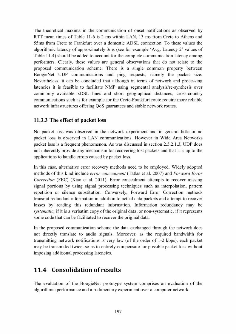
197
The theoretical maxima in the communication of onset notifications as observed by
RTT mean times of Table 11-6 is 2 ms within LAN, 13 ms from Crete to Athens and
55ms from Crete to Frankfurt over a domestic ADSL connection. To these values the
algorithmic latency of approximately 3ms (see for example ‘Avg. Latency 2’ values of
Table 11-4) should be added to account for the complete communication latency among
performers. Clearly, these values are general observations that do not relate to the
proposed communication scheme. There is a single common property between
BoogieNet UDP communications and ping requests, namely the packet size.
Nevertheless, it can be concluded that although in terms of network and processing
latencies it is feasible to facilitate NMP using segmental analysis/re-synthesis over
commonly available xDSL lines and short geographical distances, cross-country
communications such as for example for the Crete-Frankfurt route require more reliable
network infrastructures offering QoS guarantees and stable network routes.
11.3.3 The effect of packet loss
No packet loss was observed in the network experiment and in general little or no
packet loss is observed in LAN communications. However in Wide Area Networks
packet loss is a frequent phenomenon. As was discussed in section 2.5.2.1.3, UDP does
not inherently provide any mechanism for recovering lost packets and that it is up to the
applications to handle errors caused by packet loss.
In this case, alternative error recovery methods need to be employed. Widely adopted
methods of this kind include error concealment (Tatlas et al. 2007) and Forward Error
Correction (FEC) (Xiao et al. 2011). Error concealment attempts to recover missing
signal portions by using signal processing techniques such as interpolation, pattern
repetition or silence substitution. Conversely, Forward Error Correction methods
transmit redundant information in addition to actual data packets and attempt to recover
losses by reading this redundant information. Information redundancy may be
systematic, if it is a verbatim copy of the original data, or non-systematic, if it represents
some code that can be facilitated to recover the original data.
In the proposed communication scheme the data exchanged through the network does
not directly translate to audio signals. Moreover, as the required bandwidth for
transmitting network notifications is very low (of the order of 1-2 kbps), each packet
may be transmitted twice, so as to entirely compensate for possible packet loss without
imposing additional processing latencies.
11.4 Consolidation of results
The evaluation of the BoogieNet prototype system comprises an evaluation of the
algorithmic performance and a rudimentary experiment over a computer network.
198
The evaluation of the algorithmic performance focused on monitoring onset detections
using the algorithms of offline audio segmentation and HMM score following as these
were described in the corresponding chapters and implemented in the final prototype
system. Standard MIREX evaluation measures were used to inform the performance of
these algorithms. As MIREX evaluation datasets are not publicly available due to
copyright restrictions, a small music dataset was assembled and manually annotated for
the purposes of this evaluation. This dataset is significantly smaller than MIREX
datasets and therefore it is not possible to perform meaningful comparisons between the
algorithms implemented in the BoogieNet prototype and those evaluated by MIREX.
Table 11-7: Summary of the dataset and the evaluation results for the task of onset detection for MIREX 2013
and for the present evaluation.
MIREX 2013 BoogieNet
Task Audio Onset Detection OAS Dataset
Number of pieces 85 23
Total Duration 14 min 9.62 min
Number of notes NOT REPORTED 969
Results
Average for the 11 algorithms
-
Average F-measure 0.74 0.93
Average precision 0.79 0.93
Average recall 0.76 0.93
Nevertheless, the results of the present evaluation provide some preliminary findings
concerning the algorithms under evaluation. Table 11-7 summarizes properties of the
music dataset and results of the offline segmentation process of the BoogieNet
prototype aligned with those of the MIREX 2013 contest for the task of Audio Onset
Detection. Table 11-8 shows a summary of data and results for the evaluation of the
Real-time Audio to Score Alignment task, performed by MIREX 2013 and the
BoogieNet HMM score following algorithm, after HMM training. Compared to MIREX
2013 evaluation results, the offline audio segmentation process of BoogieNet resulted in
higher values for the metrics Precision, Recall and F-measure, while for score following
roughly equivalent values of piecewise and overall precision rates have been observed.
It is emphasized that a fair amount of degradation should be expected when evaluating
on larger datasets, therefore the performance of the BoogieNet algorithms could be
lower than that of the algorithms evaluated in MIREX 2013 contests.
Concerning, the facilitation of these algorithms for the intended scenario on NMP, the
network experiment revealed the following aspects. Firstly, in terms of bandwidth a 50
bytes network frame is transmitted every time an onset is detected. This comprises 42
bytes header overhead and 8 bytes of actual data. Hence, at an extreme estimate of
having four semiquavers (sixteenth notes) per beat at the tempo of 200bpm the
bandwidth consumption would be 5.3kbps (four times the rate reported on Table 11-5).
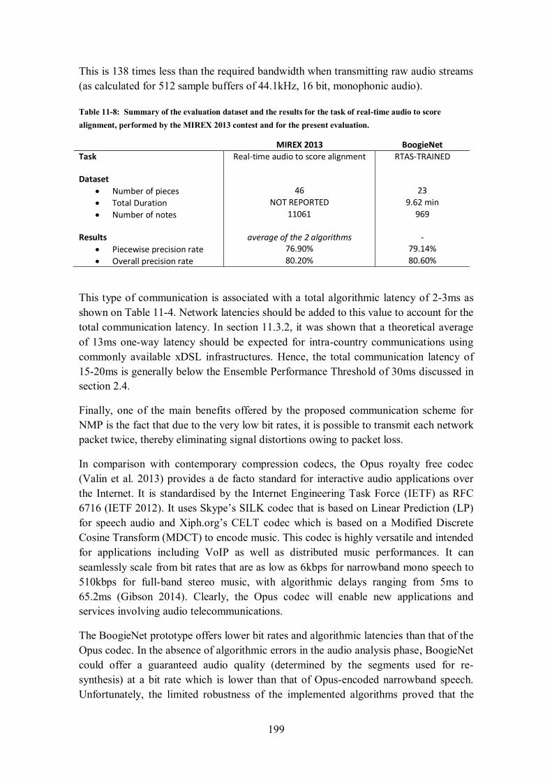
199
This is 138 times less than the required bandwidth when transmitting raw audio streams
(as calculated for 512 sample buffers of 44.1kHz, 16 bit, monophonic audio).
Table 11-8: Summary of the evaluation dataset and the results for the task of real-time audio to score
alignment, performed by the MIREX 2013 contest and for the present evaluation.
MIREX 2013 BoogieNet
Task
Real-time audio to score alignment RTAS-TRAINED
Dataset
Number of pieces 46 23
Total Duration NOT REPORTED 9.62 min
Number of notes 11061 969
Results
average of the 2 algorithms
-
Piecewise precision rate 76.90% 79.14%
Overall precision rate 80.20% 80.60%
This type of communication is associated with a total algorithmic latency of 2-3ms as
shown on Table 11-4. Network latencies should be added to this value to account for the
total communication latency. In section 11.3.2, it was shown that a theoretical average
of 13ms one-way latency should be expected for intra-country communications using
commonly available xDSL infrastructures. Hence, the total communication latency of
15-20ms is generally below the Ensemble Performance Threshold of 30ms discussed in
section 2.4.
Finally, one of the main benefits offered by the proposed communication scheme for
NMP is the fact that due to the very low bit rates, it is possible to transmit each network
packet twice, thereby eliminating signal distortions owing to packet loss.
In comparison with contemporary compression codecs, the Opus royalty free codec
(Valin et al. 2013) provides a de facto standard for interactive audio applications over
the Internet. It is standardised by the Internet Engineering Task Force (IETF) as RFC
6716 (IETF 2012). It uses Skype’s SIL codec that is based on Linear Prediction (LP)
for speech audio and Xiph.org’s CELT codec which is based on a Modified Discrete
Cosine Transform (MDCT) to encode music. This codec is highly versatile and intended
for applications including VoIP as well as distributed music performances. It can
seamlessly scale from bit rates that are as low as 6kbps for narrowband mono speech to
510kbps for full-band stereo music, with algorithmic delays ranging from 5ms to
65.2ms (Gibson 2014). Clearly, the Opus codec will enable new applications and
services involving audio telecommunications.
The BoogieNet prototype offers lower bit rates and algorithmic latencies than that of the
Opus codec. In the absence of algorithmic errors in the audio analysis phase, BoogieNet
could offer a guaranteed audio quality (determined by the segments used for re-
synthesis) at a bit rate which is lower than that of Opus-encoded narrowband speech.
Unfortunately, the limited robustness of the implemented algorithms proved that the

200
intended scenario was over-optimistic. However, it is envisaged that this research work
suggests a new and previously undermined research direction that will be realized in
upcoming developments.
201
12 Conclusions
This chapter summarizes the work presented in this dissertation, outlines contributions
and discusses various innovative perspectives in networked music research emerging
from recent achievements in the domain of machine musicianship.
12.1 Summary and concluding remarks
This dissertation proposes a novel scheme for audio communication in synchronous
musical performances carried out over computer networks. The research approach uses
techniques inspired from computer accompaniment systems, in which a software agent
follows the performance of a human musician in real-time, by synchronizing a pre-
recorded musical accompaniment to the live performance. In networked settings, each
performer participating in the distributed session is represented by a software agent,
which adapts a pre-recorded solo performance of each musician to the live music
performed at the corresponding remote location. Hence, this research focuses on the
development of software agents supporting networked music performances by their
ability to autonomously listen to the performance of each musician, notify remaining
collaborators and perform the live music based on the received notifications.
This writing builds up from contemporary musicological perspectives enabled by the
proliferation of digital media and the wide availability of network communications in
Chapter 1, the ‘Introduction’. It is shown that technological achievements have severely
altered the way music is created, distributed and analysed with respect to overcoming
conventional limitations, as well as permitting new and previously unforeseen
possibilities for interacting with musical content. Concerning music analysis,
innovations have permitted analysing music on the sound level rather than conventional
score based analysis. Sound essentially captures all expressive aspects of music
performance including expressive deviations from a predefined musical score.
Computational sound analysis allows for unambiguously observing these deviations
both at the note level (e.g. note articulations, rhythmic deviations) as well as at higher-
levels including the development of strategies for shaping a musical phrase or an entire
movement during performance. Collectively, these observations allow investigating
traditional theories on perception and cognition of musical meaning. Based solely on
signal observations, machine learning processes allow modelling expressive
performance using mathematical models. Although such models do not directly
translate to the cognitive processes undertaken by humans, they manage to successfully
deliver musical semantics in response to sound stimuli. An interesting perspective in
this direction is to develop computer musicians capable of predicting or anticipating the
future evolution of a music performance, hence simulating anticipatory processes such
202
as those taking place in the collaboration among the members of a performance
ensemble. Computational models for musical anticipation can considerably alleviate
communication problems especially when music performers are physically separated.
Following, Chapter 2 entitled ‘Networked Music Performance’ provides an overview of
research and development efforts in this domain. The chapter initially provides a brief
historical overview of research initiatives and discusses that, although expert musicians
become sceptical about remote performance collaboration, experimentalists have always
been intrigued with the idea of musical interplay across distance. The chapter outlines
the main research challenges manifested in this research domain by distinguishing
between technical impediments and collaboration deficiencies. With respect to technical
impediments, the most important obstacle impeding wide availability of NMP is the
latency observed in the communication among musicians. It is discussed that the total
communication latency comprises local latencies at the location of the transmitter and
the receiver of digital media, as well as network latencies owing to volatile network
paths and the actual geographical distance separating musicians. A separate section is
devoted to studies attempting to measure latency tolerance in ensemble performance,
known as Ensemble Performance Threshold (EPT), hence implicitly delineating the
temporal limits of performers’ musical anticipation. These studies acknowledge that the
precise value of the EPT depends on characteristic properties of the music being
performed (e.g. tempo, instrumentation), however in most cases they agree that for
uninterrupted ensemble performance communication latencies should not exceed an
approximate value of 30ms. Following, the chapter outlines the fundamental
constituents of an NMP system in terms of software architectures and network
infrastructures. This description permits tracing potential causes of technical
impediments throughout the entire route of real-time audio communication. Finally in
terms of collaboration deficiencies, it is shown that developing intelligent user
interfaces for NMP, subsuming machine listening capabilities, can significantly improve
the experience of musicians and foster a plethora of novel perspectives in computer-
assisted musical collaboration.
Machine musicianship is discussed in Chapter 3. The chapter begins by defining the
terms machine listening and machine musicianship and further distinguishing between
computational approaches with the objective of understanding musical cognition in
humans and those aiming at extrapolating meaningful information from audio signals to
be further used in a wide range of practical software applications. Then, the overall
methodology followed by machine listening and auditory scene analysis systems is
described using examples on how they are realized in different disciplines concerning
speech, environmental sounds and music. The section that follows focuses on four
functionalities of machine musicianship, namely on automatic music transcription,
audio to score alignment, audio synchronisation and computer accompaniment. For
each of these functionalities, existing research initiatives and computational techniques
are discussed so as to provide a baseline for the possibilities available for
experimentation with the research approach under investigation. Finally, the chapter is
203
concluded by discussing that - at the time of this writing - there are very few research
initiatives attempting to exploit machine musicianship in the context of NMP.
An additional research domain considered relevant to the present work, is that of
Concatenative Sound Synthesis (CSS) and it is presented in Chapter 4. The objective of
CSS systems is to generate a waveform by concatenating segments of pre-recorded
sound material, given a target specification (most commonly provided as an audio
stream or a symbolic representation, e.g. a score), so that the resulting waveform will
optimally resemble the target, in some sense which depends on the target application.
Initially, the chapter presents the overall methodology employed by CSS systems and
the alternative computational techniques that have been facilitated in different
applications and reported in the relevant literature. As this type of sound synthesis
originates from speech synthesis systems, a brief overview of relevant speech synthesis
and coding techniques is additionally provided. Following, the chapter concentrates on
music synthesis and some of the most popular approaches are presented and contrasted
with the synthesis method to be implemented for the intended communication in NMP.
The chapter concludes by showing that none of the currently popular CSS approaches
attempts to satisfy all three challenges confronted by the system under investigation,
which are the requirement for high quality instrumental synthesis, the fact that the target
to be synthesis is provided as an audio signal (hence requiring prior analysis) and the
fact that analysis of target and re-synthesis needs to take place within strict time
constraints imposed by the EPT.
The remaining part of the dissertation provides details on the research and development
efforts carried out for the purposes of implementing the intended communication
scheme for distributed music collaborations.
Chapter 5 describes this research objective and presents the challenges to be confronted
including strict real-time requirements, constrained not only in terms of using causal
algorithmic processes, but also by restricting the total end-to-end communication delay
that needs to be kept below the EPT. Concerning benefits, it is deduced that if the
algorithms implementing the functionalities of ‘listening’ and ‘performing’ can become
sufficiently robust, this type of communication can provide superior sound quality
compared to alternative low bit-rate communication of music, such as MIDI.
Equivalently, assuming that the algorithmic complexity of the proposed scheme can be
effectively reduced to accommodate the requirement of the EPT, communication based
on note notifications can prove more efficient, in terms of network resource
consumption, than facilitating audio compression schemes. Following, a number of
assumptions/prerequisites are set on the usage scenario, so as to allow early
investigations carried out in the present dissertation to produce some useful research
results. These assumptions are mainly concerned with the fact that the signals to be
analysed are constrained to mono-timbral and monophonic music and that the
performance needs to be a precise interpretation of a pre-defined music score. The last
section presents the block diagram of the entire prototype system to be developed.

204
The next chapter is devoted to audio features. It is intended as a reference for the
chapters that follow and it provides definitions for a number of audio features that are
commonly used in audio segmentation and machine listening research. Besides
mathematical definitions, the chapter attempts to provide insight to the expected
temporal behaviour of the various features. This is achieved using diagrams depicting
the evolution of audio features for an example musical phrase. Possibly the most
significant contribution of this chapter is a discussion on the importance of the
parameterisation of the Fourier transform when computing spectral features intended for
real-time music analysis. Specifically, it is shown that as audio should be captured in
sufficiently small chunks to mitigate the effect of long buffering delays, zero-padding
may be preferred to highly overlapping analysis windows, as it increases the
contribution of each chunk to the overall spectral energy. Moreover, it is shown that a
rectangular windowing functions may be more appropriate to a bell-shaped window
when the emphasis is on early onset detection. Specifically, an onset occurring at the
location of a ‘window-hop’ may be dumped due to windowing functions that are
smoothly attenuating the amplitude near the boundaries of the analysis window, where
the hop actually occurs. It is therefore more likely that indications of sudden energy
bursts are detected earlier in the signal, when using a rectangular window.
Subsequently, chapter 7 is devoted to the offline audio segmentation process. This
process aims at automatically generating a pool of audio segments, each corresponding
to a different note of the solo recording of each musician participating in an NMP
session. During NMP, these segments are transformed in terms of duration and
amplitude and appropriately concatenated to re-synthesize the performance of each
musician at the location of remote collaborators. The chapter initially discusses the
acoustic characteristics of note onsets and how these diverge depending on the
instrument timbre as well as on expressive articulation. It is discussed that the relevant
literature distinguishes between two types of onsets, namely salient onsets associated
with strong transients corresponding to energy bursts in the high frequency spectrum
and subtle onsets that do not exhibit such abrupt behaviour and correspond to smooth
sound generation mechanisms or subtle pitch changes. Following the general
methodology of blind onset detection algorithms is presented in three steps (i.e. pre-
processing, reduction and peak-picking) along with representative examples of how
these steps have been implemented in previous research initiatives. Finally, the chapter
presents the offline audio segmentation algorithm that was devised and implemented in
the final software prototype. It is shown that this algorithm is informed by the number
of notes that need to be found (as provided by the corresponding score of the music
piece) and that subtle onsets are detected using instantaneous pitch detection by means
of a wavelet transform. In comparison with conventional onset detection algorithms,
these two aspects are intended to increase the robustness of onset detections for a wide
variety of instrument timbres and expressive articulations.
Chapter 8 is devoted to the methodology followed for the purposes of tracking the
performance of each musician in real-time. This represents the ‘listening’ component of
205
the system. As listening is achieved by means of HMM score following, the chapter
provides an elaborate discussion on the mathematical representation of these models. Of
particular importance is a section devoted to design considerations manifested when
developing HMMs for machine listening tasks. This includes a number of challenges I
was confronted with, during extensive experimentation with various model
representations. Among other things, the section discusses HMM topologies, and
problems related to numerical instability, increased memory requirements and the lack
of sufficient data to effectively train such models. This discussion is informed by
examples of how these problems have been approached in the relevant literature and the
workarounds I employed in my implementation, so as to increase the computational
performance of the real-time performance tracking component. Finally, implementation
specific details are recapitulated in the last section, which additionally presents the
block diagrams for the processes of HMM training and the real-time decoding.
Chapter 9 presents the methodology followed for re-synthesizing the live performance
of each musician by using the segments of a prior solo recording. This constitutes the
‘performing’ component of the system. The employed methodology is called segmental
re-synthesis, so as to avoid confusion with well-known concatenative sound synthesis
approaches. The chapter initially elaborates on relevant studies in expressive music
performance. It is argued that there are numerous possibilities in deviating from mere
score rendition, including the timing of different events, chord asynchronies, slight pitch
deviations, variations in dynamics, note articulations and so on. It is discussed that, in
line with Meyer’s (1956) notion of structural meaning, most of these studies emphasize
on the importance of musical structure driving performers’ intentions with respect to
musical expression. The most conscious and readily tractable expressive nuances are
concerned with loudness and tempo variations within a melodic or harmonic
progression. Consequently, these are the main properties addressed in expression-aware
audio systems. The chapter also discusses that applying audio transformations in
expressive musical collaboration, as for example in computer accompaniment systems,
necessitates the implementation of anticipatory processes predicting the transformations
that need to be applied prior to rendering, similarly to the musical anticipation occurring
between the members of a performance ensemble. Then, the chapter provides an
overview of the most widely used waveform time-scaling techniques, which are the
phase vocoder and the PSOLA transforms, and presents the approach implemented in
the context of this work, regarding the anticipation of expressive deviations, amplitude
and time-scaling transformations as well as techniques for eliminating signal
discontinuities at the junction point of consecutive audio segments.
The remaining two chapters are devoted to the implementation details and the
experimental evaluation of the software prototype that was implemented as a result of
this doctoral research.
Chapter 10 describes the implementation of this software framework. It is given the
name BoogieNet and it has been implemented in C++. BoogieNet is downloadable from
206
a personal webpage as open source software, packaged using a GNU/GPL license. The
chapter provides a user manual, for researchers wishing to experiment with this
framework and further describes its object-oriented design in terms of the implemented
classes and some associated text files that are generated by the software. Finally, the
chapter lists all third party libraries that have been used in the implementation of
BoogieNet.
Chapter 11 presents the evaluation of the BoogieNet software prototype. Specifically,
BoogieNet has been evaluated for its algorithmic performance in the machine listening
task, comprising the functionalities of offline audio segmentation and HMM score
following as well as for its efficiency in terms of network resource consumption, in
permitting music performers to communicate across distance. Algorithmic performance
has been evaluated on a small dataset of solo monophonic instrument performances
comprising 23 music pieces. In terms of actual performance measures it was shown that
BoogieNet yields a similar performance, to onset detection and score following
algorithms reported in the relevant literature. Specifically, it was shown that as the
results of the offline audio segmentation process are further used for initialising the
HMM model for each music piece, the performance of the score following algorithm is
determined by that of the offline segmentation. Errors of the offline segmentation
process are propagated to the score following process, yielding an approximate 25%
degradation in the number of correct detections. Although the score following algorithm
has a performance that is suboptimal to that of audio segmentation, it was found that
training the model prior to real-time decoding improves the performance of real-time
decoding by an approximate factor of 12%. To statistically confirm this fact, a
significance test revealed a 95% significance of the hypothesis that the implementation
of the Baum-Welch algorithm for training the HMM, improves the performance of
score following compared to the performance achieved prior to Baum-Welch training.
With respect to evaluating different instrument timbres, it was shown that the offline
audio segmentation algorithm yields superior performance for percussive instruments
and reaches the minimum of its performance for bowed string instruments. This does
not hold for the score following process which is heavily dependent on pitch
information. Non-chromatic percussive instruments produce highly in-harmonic sounds
and therefore the observation probabilities of the HMM should not rely on pitch
information. Finally, the algorithm for segmental re-synthesis was not evaluated for
algorithmic performance, however it was discussed that the main shortcoming of its
current implementation is the fact that time-scaling transformations assume that the
offline segmentation process is fully accurate. Errors introduced during offline audio
segmentation will result in distortions on the synthesised signal. Thus, a more robust
approach needs to be incorporated both for the anticipation of expressive deviations in
music performance as well as for time scaling the pre-existing solo recording.
In addition to experiments evaluating the algorithmic performance of BoogieNet, a
network experiment was conducted to provide some insight the expected network
207
traffic, while disregarding errors in algorithmic performance. It was elucidated that the
proposed communication scheme has a variable bit rate, which depends on the rate of
detected onsets. The implemented UDP communication mechanism results in a separate
network packet of 50 bytes transmitted at every onset detection. It is discussed that the
actual bit-rate may be computed based on the instant tempo and the score structure, as a
function of the number of the score events per second. It is for example estimated that
having four semiquavers per beat at a tempo of 200bpm will result in an expected bit
rate of 5.3kbps. In comparison, transmitting monophonic audio of CD quality requires
730kbps. As for audio compression, the Opus codec, which is the present state of the art
in low-latency and low-bit rate communication, requires a minimum bit rate of 6kbps
for speech quality audio. Hence, in terms of bandwidth consumption the proposed
scheme is superior to alternative state of the art schemes in audio communication.
However, the benefits offered by the BoogieNet approach are not really on bandwidth
consumption, but rather on extremely low algorithmic complexity, resulting in
processing latencies of up to 3ms and the fact that, as the communication bit rate is very
low, it is possible to transmit multiple replicas of each notification, so as to entirely
alleviate from the effects of network packet loss. Latencies owing to network
transmission are not directly addressed by the present work, as the proposed
optimisations are not related to network routes or communication protocols. However,
low algorithmic delays in the lifecycle of an audio chuck, allow for accommodating
higher delays during transmission. Respecting the value of the EPT, this results in a
range of allowable transmission delays up to approximately 27ms. Using ping requests
that provide a theoretical maximum on transmission delays, it was found that this is in
the range of expected delays when using xDSL connections and geographical distances
that are roughly within the same country. However, in cross-country communications,
as for example between Greece and Germany, it is necessary to also apply optimisations
on the network paths. Nevertheless, allowing intra-country communications using
commonly available xDSL lines and complete elimination of the effects of network
packet loss, offers a significant advantage in the communication of music collaborators.
12.2 Contributions
The main contribution of this work is the investigation of a novel paradigm for musical
collaboration across computer networks and it is encapsulated in the implementation of
the BoogieNet software prototype. This prototype has been made available as open
source software, hoping that researchers and practitioners will be keen to experiment
with the proposed idea and further contribute to the realisation of this type of artificially
intelligent musical communications. To increase visibility, this work has been presented
and published in the proceedings of two international conferences (Alexandraki and
Bader 2014; Alexandraki and Bader 2013).
The following list recapitulates some contributions and findings of this work:
208
An elaborate discussion on the importance of the parameterisation of the Fourier
transform when it is used for extrapolating musical information in real-time
context, as described in section 6.3.
An offline onset detection algorithm, presented in section 7.4.1, which takes into
account both salient onsets, associated with strong initial transients, as well as
subtle pitch changes.
An elaborate discussion on design issues to consider when implementing HMMs
for music performance following, in section 8.3.
An implementation of an HMM score following algorithm for monophonic
instruments, presented in section 8.4
A new method for lightweight low-distortion time scaling of monophonic music,
informed by the timing of note onsets and their pitch frequencies, presented in
section 9.3.2
Although, offering robust and unconstraint communication in music performance using
the proposed scheme is still a long way off, this dissertation is a first step towards this
important long-term goal. Throughout various investigations it was found out that
realizing the intended scenario was highly optimistic in terms of the expected
algorithmic performance of the audio analysis algorithms. It was shown, that like the
main bulk of Music Information Retrieval research initiatives, the algorithms
implemented in BoogieNet cannot fully cope with the abundance of timbral and
temporal complexities introduced in the music performance of acoustic instruments and
human musicians. Although the implemented algorithms achieve to successfully
recognize the majority of musical events, they are not meant to be 100% robust.
This is probably the most outstanding challenge encountered when aiming to derive
perceptually meaningful information using mathematical models and computational
prototyping. No such algorithm can fully model the complexities of the human brain.
Therefore, when aiming to develop applications that require high accuracy, emphasis
should be given to copying with inaccuracies. This can be done either by integrating
human knowledge in the implementation of these models, for example heuristics rules,
or by implementing algorithms that are able detect their failures and re-adjust their
parameters during functional operation, i.e. without failing to carry on .
12.3 Implications, shortcomings and future perspectives
The motivation of the work presented in this dissertation lies in the development of a
system which will be able to progressively learn and model the individualities of each
performer, with respect to music expression. The original idea was to implement an
artificial ‘clone’ of each musician, capable of developing musical skills and increasingly
improving its resemblance to the human performer though continuous use. In such an
ideal scenario, musicians would be able to travel with their clones and use them to
collaborate with their peers from different locations across the globe.
209
This vision raised a number of questions, clearly not possible to address within the time
limits of a doctoral dissertation. For example, is it possible to formulate general rules of
how performers develop strategies to shape their personal interpretation of any given
music work? What are the distinguishing characteristics of each individual performance
of the same music work when it is performed by the same artist? In other words, what
are the parameters that are susceptible to change from one performance to another?
How does collaboration between the members of a performance ensemble reshape one’s
own intentions with respect to musical expression? As already elaborated in various
places within this dissertation, there is an abundance of possibilities in deviating from
faithful score rendition. Is it possible to define subsets of such deviations that are more
commonly adopted by certain artists? If so, how could these personal deviations relate
to the actual structure residing in a music piece?
It is well known that expressive performance is an extremely complex cognitive and
artistic phenomenon, not possible to explain using general rules. In this regard, two
research tendencies are being pursuit: the one aiming at understanding the specificities
of this complex phenomenon and that aiming at developing expression-aware audio
systems. It may be argued that artificial intelligence and inductive machine learning
applied on large music corpora can provide successful developments of expression-
aware audio systems, without requiring full comprehension of the underlying
mechanisms of music perception. Nevertheless, and almost by definition, the maximum
performance that can be achieved by machine learning models will always be
suboptimal to our perception of music. A plausible question in this direction relates to
whether inaccuracies of such models lead to systems failing to deliver their intended
functionality.
The perspective investigated in this dissertation falls in this category of highly
challenging applications, with respect to the required accuracy of the algorithms of
machine listening and expression-aware audio rendering. This is probably the reason
why the proposed perspective has not been previously investigated and the reason why
the most popular applications of inductive machine learning in music are concerned
with either music similarity and recommendation or with general purpose beat tracking,
chord recognition, music transcription etc., thereby presenting solutions that are less
vulnerable to algorithmic failures. It is likely that certain applications, such as the one
investigated here, require a better understanding of human psychology and cognition in
order to cope with the inaccuracies of mathematical models and recover from
algorithmic failures. Yet, the performance model generated for each musician by the
system implemented here may be regarded as a ‘fingerprint’, which is unique to each
particular performer and therefore encapsulates all distinctive aspects of his/her own
understanding to music expression.
Ultimately, there are a number of shortcomings in the present work, to be addressed in
ongoing and future research efforts. These shortcomings have been discussed in
210
different places within the document and they are summarised here, along with some
ideas on how they can be addressed in future developments.
The most important limitations of the current approach are outlined in the pre-requisites
that were set forth during the initial phases of research investigations (section 5.3). For
instance, one straightforward extension of the investigated algorithms is to
accommodate polyphonic, in addition to monophonic, musical instruments. At present,
there are numerous research works addressing polyphonic music alignment (e.g. Hu,
Dannenber and Tzanetakis 2003; Soulez, Rodet and Schwarz 2003; Niedermayer 2009),
with a few of them presenting online and real-time approaches (e.g. Otsuka et al. 2011,
Duan and Pardo 2011a; Montecchio and Cont 2011a; Cont 2010). However, these
works do not clearly address real-time constraints in terms of the time taken by the
system to respond to an alignment decision.
Notably, recent approaches to score scrolling and real-time audio synchronisation
increasingly suggest Particle Filter based models instead of conventional DTW or
HMM approaches. Particle Filters approaches were briefly discussed in section 3.2.2
and offer several advantages over conventional models, including the fact that they are
capable of modelling both audio-to-audio as well as audio-to-score alignments, they are
highly efficient in real-time operation, they are robust to performance discrepancies
both at the note level as well as the structural level (e.g. omitted repetitions) (Xiong and
Izmirli 2012), and also the fact that they do not require prior training.
In fact, an alternative approach to the one investigated in this dissertation would be to
implement a Particle Filter solution to directly align the live recording of each
performer to the pre-existing solo recording, thus alleviating from the requirement of
obtaining a score representation of the piece to be performed. As there is evidence that
Particle Filters can cope with performance deviations, including performance errors,
such an approach would alleviate from an additional deficiency of the current
implementation, which is concerned with the fact that performers are assumed to
precisely interpret the score without any errors. Clearly, this is a rather ideal situation
that rarely ever occurs. The employed algorithms need to take into account performance
errors as well as the fact that, in cases where collaboration occurs for the purposes of a
music rehearsal, a music lesson or an improvisation session, musicians will occasionally
stop before the end or repeatedly perform certain phrases or sections within a music
piece.
Finally with respect to real-time re-synthesis, it could have been more appropriate to
time stretch or otherwise transform the original solo recording without prior
segmentation and segment concatenation, in a similar approach to the one employed for
example by Raphael (2003). In this case, phase vocoder time-scaling techniques offer a
widely adopted solution. However, the reason for choosing prior segmentation and
segment concatenation in the present investigations originates from the initial idea of
ultimately allowing a performer to perform arbitrary music pieces and facilitating a data
corpus to re-synthesize one’s expressive performance from previously recorded phrases

211
or note articulations of that same performer and do so in real-time. Time-stretching a
pre-existing recording would preclude the possibility of employing the proposed
communication scheme for improvisational music. In contrast, when concatenating
small segments of audio, any audio stream can be potentially rendered by means of
concatenative sound synthesis. Hence, in terms of segmental re-synthesis, future
research efforts are oriented towards generating a larger and appropriately annotated
audio corpus for each musician and implementing algorithms for real-time unit
selection. This also gives greater flexibility to the types of interpreted nuances that may
be accommodated by the proposed approach.
Clearly, there are endless possibilities in experimenting with the idea of communicating
performance intentions, to be rendered at remote locations. These perspectives demand
further research on how to encode or represent such intentions and how to process
existing signals to more appropriately reflect these intentions. This could go up to
modelling the cognitive skills employed when developing music improvisation
strategies (William and Wallace 2004; Pressing 1987), human-computer music
improvisation (Young 2010; Walker 1997) or even computer musicians autonomously
collaborating from distance with or without human supervision controlling the evolving
musical structures.
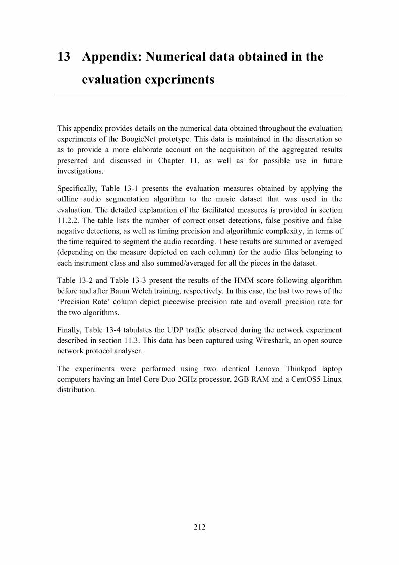
212
13 Appendix: Numerical data obtained in the
evaluation experiments
This appendix provides details on the numerical data obtained throughout the evaluation
experiments of the BoogieNet prototype. This data is maintained in the dissertation so
as to provide a more elaborate account on the acquisition of the aggregated results
presented and discussed in Chapter 11, as well as for possible use in future
investigations.
Specifically, Table 13-1 presents the evaluation measures obtained by applying the
offline audio segmentation algorithm to the music dataset that was used in the
evaluation. The detailed explanation of the facilitated measures is provided in section
11.2.2. The table lists the number of correct onset detections, false positive and false
negative detections, as well as timing precision and algorithmic complexity, in terms of
the time required to segment the audio recording. These results are summed or averaged
(depending on the measure depicted on each column) for the audio files belonging to
each instrument class and also summed/averaged for all the pieces in the dataset.
Table 13-2 and Table 13-3 present the results of the HMM score following algorithm
before and after Baum Welch training, respectively. In this case, the last two rows of the
‘Precision Rate’ column depict piecewise precision rate and overall precision rate for
the two algorithms.
Finally, Table 13-4 tabulates the UDP traffic observed during the network experiment
described in section 11.3. This data has been captured using Wireshark, an open source
network protocol analyser.
The experiments were performed using two identical Lenovo Thinkpad laptop
computers having an Intel Core Duo 2GHz processor, 2GB RAM and a CentOS5 Linux
distribution.
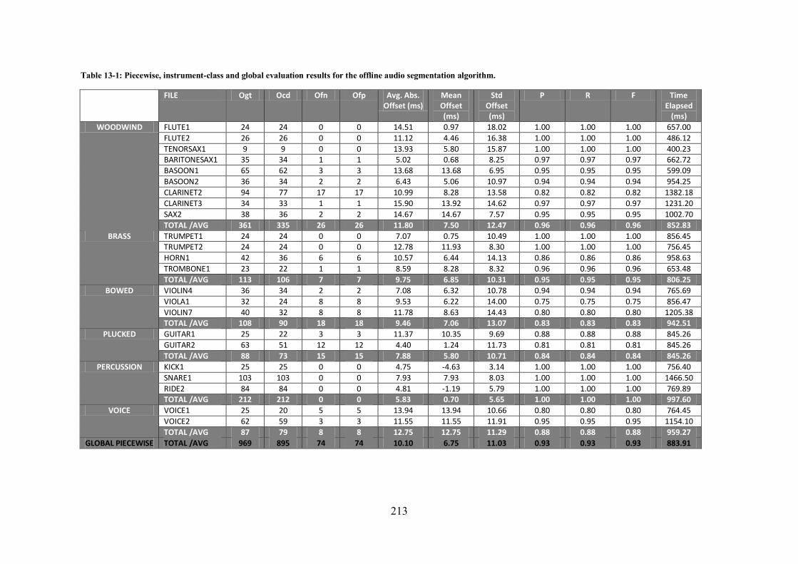
213
Table 13-1: Piecewise, instrument-class and global evaluation results for the offline audio segmentation algorithm.
FILE Ogt Ocd Ofn Ofp Avg. Abs. Offset (ms)
Mean Offset (ms)
Std Offset (ms)
P R F Time Elapsed
(ms)
WOODWIND FLUTE1 24 24 0 0 14.51 0.97 18.02 1.00 1.00 1.00 657.00
FLUTE2 26 26 0 0 11.12 4.46 16.38 1.00 1.00 1.00 486.12
TENORSAX1 9 9 0 0 13.93 5.80 15.87 1.00 1.00 1.00 400.23 BARITONESAX1 35 34 1 1 5.02 0.68 8.25 0.97 0.97 0.97 662.72
BASOON1 65 62 3 3 13.68 13.68 6.95 0.95 0.95 0.95 599.09
BASOON2 36 34 2 2 6.43 5.06 10.97 0.94 0.94 0.94 954.25
CLARINET2 94 77 17 17 10.99 8.28 13.58 0.82 0.82 0.82 1382.18
CLARINET3 34 33 1 1 15.90 13.92 14.62 0.97 0.97 0.97 1231.20
SAX2 38 36 2 2 14.67 14.67 7.57 0.95 0.95 0.95 1002.70
TOTAL /AVG 361 335 26 26 11.80 7.50 12.47 0.96 0.96 0.96 852.83
BRASS TRUMPET1 24 24 0 0 7.07 0.75 10.49 1.00 1.00 1.00 856.45 TRUMPET2 24 24 0 0 12.78 11.93 8.30 1.00 1.00 1.00 756.45
HORN1 42 36 6 6 10.57 6.44 14.13 0.86 0.86 0.86 958.63
TROMBONE1 23 22 1 1 8.59 8.28 8.32 0.96 0.96 0.96 653.48
TOTAL /AVG 113 106 7 7 9.75 6.85 10.31 0.95 0.95 0.95 806.25
BOWED VIOLIN4 36 34 2 2 7.08 6.32 10.78 0.94 0.94 0.94 765.69
VIOLA1 32 24 8 8 9.53 6.22 14.00 0.75 0.75 0.75 856.47
VIOLIN7 40 32 8 8 11.78 8.63 14.43 0.80 0.80 0.80 1205.38 TOTAL /AVG 108 90 18 18 9.46 7.06 13.07 0.83 0.83 0.83 942.51
PLUCKED GUITAR1 25 22 3 3 11.37 10.35 9.69 0.88 0.88 0.88 845.26
GUITAR2 63 51 12 12 4.40 1.24 11.73 0.81 0.81 0.81 845.26
TOTAL /AVG 88 73 15 15 7.88 5.80 10.71 0.84 0.84 0.84 845.26
PERCUSSION KICK1 25 25 0 0 4.75 -4.63 3.14 1.00 1.00 1.00 756.40
SNARE1 103 103 0 0 7.93 7.93 8.03 1.00 1.00 1.00 1466.50
RIDE2 84 84 0 0 4.81 -1.19 5.79 1.00 1.00 1.00 769.89 TOTAL /AVG 212 212 0 0 5.83 0.70 5.65 1.00 1.00 1.00 997.60
VOICE VOICE1 25 20 5 5 13.94 13.94 10.66 0.80 0.80 0.80 764.45
VOICE2 62 59 3 3 11.55 11.55 11.91 0.95 0.95 0.95 1154.10
TOTAL /AVG 87 79 8 8 12.75 12.75 11.29 0.88 0.88 0.88 959.27
GLOBAL PIECEWISE TOTAL /AVG 969 895 74 74 10.10 6.75 11.03 0.93 0.93 0.93 883.91
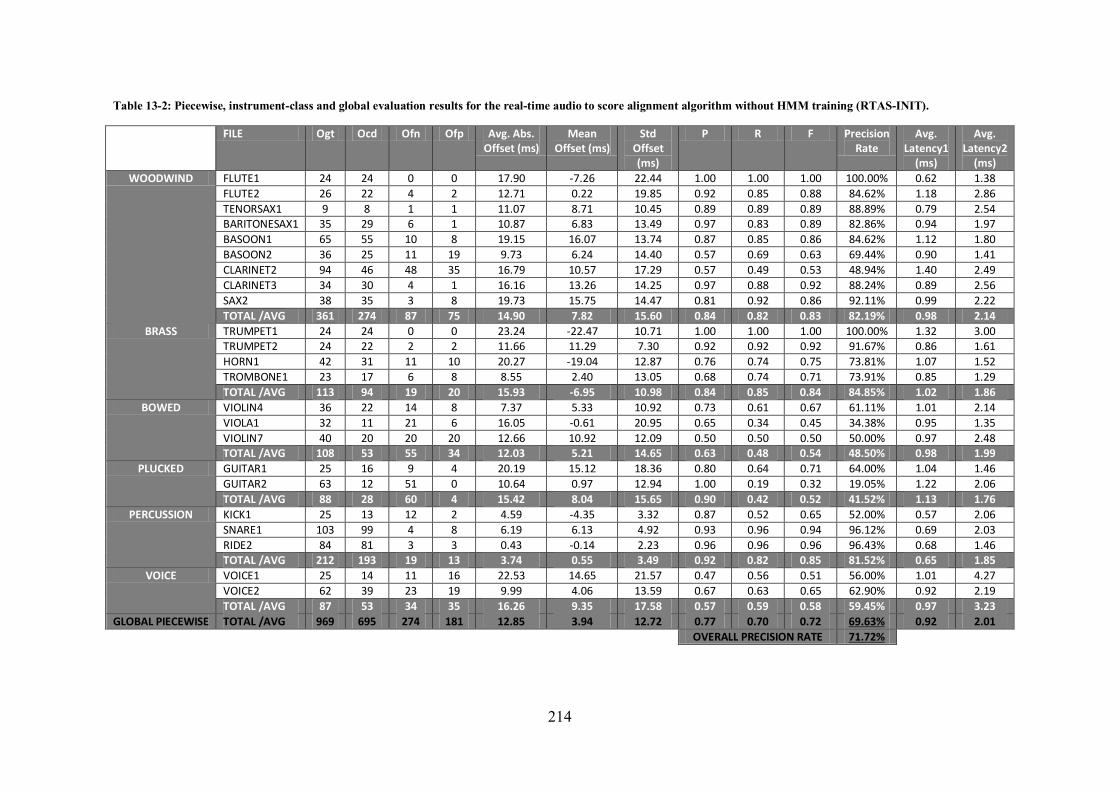
214
Table 13-2: Piecewise, instrument-class and global evaluation results for the real-time audio to score alignment algorithm without HMM training (RTAS-INIT).
FILE Ogt Ocd Ofn Ofp Avg. Abs. Offset (ms)
Mean Offset (ms)
Std Offset (ms)
P R F Precision Rate
Avg. Latency1
(ms)
Avg. Latency2
(ms)
WOODWIND FLUTE1 24 24 0 0 17.90 -7.26 22.44 1.00 1.00 1.00 100.00% 0.62 1.38
FLUTE2 26 22 4 2 12.71 0.22 19.85 0.92 0.85 0.88 84.62% 1.18 2.86
TENORSAX1 9 8 1 1 11.07 8.71 10.45 0.89 0.89 0.89 88.89% 0.79 2.54 BARITONESAX1 35 29 6 1 10.87 6.83 13.49 0.97 0.83 0.89 82.86% 0.94 1.97
BASOON1 65 55 10 8 19.15 16.07 13.74 0.87 0.85 0.86 84.62% 1.12 1.80
BASOON2 36 25 11 19 9.73 6.24 14.40 0.57 0.69 0.63 69.44% 0.90 1.41
CLARINET2 94 46 48 35 16.79 10.57 17.29 0.57 0.49 0.53 48.94% 1.40 2.49
CLARINET3 34 30 4 1 16.16 13.26 14.25 0.97 0.88 0.92 88.24% 0.89 2.56
SAX2 38 35 3 8 19.73 15.75 14.47 0.81 0.92 0.86 92.11% 0.99 2.22
TOTAL /AVG 361 274 87 75 14.90 7.82 15.60 0.84 0.82 0.83 82.19% 0.98 2.14
BRASS TRUMPET1 24 24 0 0 23.24 -22.47 10.71 1.00 1.00 1.00 100.00% 1.32 3.00 TRUMPET2 24 22 2 2 11.66 11.29 7.30 0.92 0.92 0.92 91.67% 0.86 1.61
HORN1 42 31 11 10 20.27 -19.04 12.87 0.76 0.74 0.75 73.81% 1.07 1.52
TROMBONE1 23 17 6 8 8.55 2.40 13.05 0.68 0.74 0.71 73.91% 0.85 1.29
TOTAL /AVG 113 94 19 20 15.93 -6.95 10.98 0.84 0.85 0.84 84.85% 1.02 1.86
BOWED VIOLIN4 36 22 14 8 7.37 5.33 10.92 0.73 0.61 0.67 61.11% 1.01 2.14
VIOLA1 32 11 21 6 16.05 -0.61 20.95 0.65 0.34 0.45 34.38% 0.95 1.35
VIOLIN7 40 20 20 20 12.66 10.92 12.09 0.50 0.50 0.50 50.00% 0.97 2.48 TOTAL /AVG 108 53 55 34 12.03 5.21 14.65 0.63 0.48 0.54 48.50% 0.98 1.99
PLUCKED GUITAR1 25 16 9 4 20.19 15.12 18.36 0.80 0.64 0.71 64.00% 1.04 1.46
GUITAR2 63 12 51 0 10.64 0.97 12.94 1.00 0.19 0.32 19.05% 1.22 2.06
TOTAL /AVG 88 28 60 4 15.42 8.04 15.65 0.90 0.42 0.52 41.52% 1.13 1.76
PERCUSSION KICK1 25 13 12 2 4.59 -4.35 3.32 0.87 0.52 0.65 52.00% 0.57 2.06
SNARE1 103 99 4 8 6.19 6.13 4.92 0.93 0.96 0.94 96.12% 0.69 2.03
RIDE2 84 81 3 3 0.43 -0.14 2.23 0.96 0.96 0.96 96.43% 0.68 1.46 TOTAL /AVG 212 193 19 13 3.74 0.55 3.49 0.92 0.82 0.85 81.52% 0.65 1.85
VOICE VOICE1 25 14 11 16 22.53 14.65 21.57 0.47 0.56 0.51 56.00% 1.01 4.27
VOICE2 62 39 23 19 9.99 4.06 13.59 0.67 0.63 0.65 62.90% 0.92 2.19
TOTAL /AVG 87 53 34 35 16.26 9.35 17.58 0.57 0.59 0.58 59.45% 0.97 3.23
GLOBAL PIECEWISE TOTAL /AVG 969 695 274 181 12.85 3.94 12.72 0.77 0.70 0.72 69.63% 0.92 2.01
OVERALL PRECISION RATE 71.72%

215
Table 13-3: Piecewise, instrument-class and global evaluation results for the real-time audio to score alignment algorithm after HMM training (RTAS-TRAINED).
FILE Ogt Ocd Ofn Ofp Avg. Abs. Offset (ms)
Mean Offset (ms)
Std Offset (ms)
P R F Precision Rate
Avg. Latency1 (ms)
Avg. Latency2
(ms)
WOODWIND FLUTE1 24 23 1 1 12.62 -0.50 17.28 0.96 0.96 0.96 95.83% 0.62 1.38
FLUTE2 26 22 4 2 11.83 1.81 18.18 0.92 0.85 0.88 84.62% 1.21 2.92
TENORSAX1 9 8 1 1 10.16 10.16 13.10 0.89 0.89 0.89 88.89% 0.84 2.66 BARITONESAX1 35 32 3 3 8.12 0.81 12.85 0.91 0.91 0.91 91.43% 0.91 1.95
BASOON1 65 53 12 7 18.36 15.30 13.29 0.88 0.82 0.85 81.54% 1.09 1.82
BASOON2 36 36 0 3 5.60 4.31 8.72 0.92 1.00 0.96 100.00% 0.91 1.42
CLARINET2 94 64 30 23 17.45 13.77 16.95 0.74 0.68 0.71 68.09% 1.36 8.25
CLARINET3 34 32 2 1 14.26 12.27 11.81 0.97 0.94 0.96 94.12% 0.92 2.54
SAX2 38 36 2 2 20.47 16.60 14.88 0.95 0.95 0.95 94.74% 0.99 2.39
TOTAL /AVG 361 306 55 43 13.21 8.28 14.12 0.90 0.89 0.90 88.80% 0.98 2.82
BRASS TRUMPET1 24 24 0 0 20.82 -20.05 11.71 1.00 1.00 1.00 100.00% 1.31 3.01 TRUMPET2 24 24 0 0 12.11 10.97 8.29 1.00 1.00 1.00 100.00% 0.81 1.55
HORN1 42 31 11 8 17.93 -14.35 14.33 0.79 0.74 0.77 73.81% 1.07 1.52
TROMBONE1 23 21 2 2 7.91 0.69 12.65 0.91 0.91 0.91 91.30% 0.86 1.31
TOTAL /AVG 113 100 13 10 14.69 -5.69 11.74 0.93 0.91 0.92 91.28% 1.01 1.85
BOWED VIOLIN4 36 25 11 14 7.99 3.92 10.61 0.64 0.69 0.67 69.44% 1.02 1.47
VIOLA1 32 20 12 9 12.39 8.68 14.41 0.69 0.63 0.66 62.50% 0.98 1.48
VIOLIN7 40 32 8 21 18.07 13.81 17.89 0.60 0.80 0.69 80.00% 0.97 3.13 TOTAL /AVG 108 77 31 44 12.82 8.81 14.30 0.64 0.71 0.67 70.65% 0.99 2.02
PLUCKED GUITAR1 25 19 6 10 16.02 6.39 19.21 0.66 0.76 0.70 76.00% 1.08 1.51
GUITAR2 63 38 25 10 9.97 6.91 12.52 0.79 0.60 0.68 60.32% 1.53 2.50
TOTAL /AVG 88 57 31 20 12.99 6.65 15.86 0.72 0.68 0.69 68.16% 1.30 2.01
PERCUSSION KICK1 25 22 3 6 4.67 -4.53 3.14 0.79 0.88 0.83 88.00% 0.59 1.10
SNARE1 103 73 30 13 6.60 5.39 6.35 0.85 0.71 0.77 70.87% 0.67 10.59
RIDE2 84 80 4 3 0.44 -0.44 2.21 0.96 0.95 0.96 95.24% 0.67 1.41 TOTAL /AVG 212 175 37 22 3.90 0.14 3.90 0.87 0.85 0.85 84.70% 0.64 4.36
VOICE VOICE1 25 11 14 18 20.47 13.71 21.16 0.38 0.44 0.41 44.00% 0.95 2.31
VOICE2 62 55 7 10 13.47 9.30 14.07 0.85 0.89 0.87 88.71% 0.92 2.20
TOTAL /AVG 87 66 21 28 16.97 11.51 17.61 0.61 0.66 0.64 66.35% 0.93 2.26
GLOBAL PIECEWISE TOTAL /AVG 969 781 188 167 11.99 4.79 12.32 0.79 0.79 0.79 79.14% 0.93 2.52
OVERALL PRECISSION RATE 80.60%
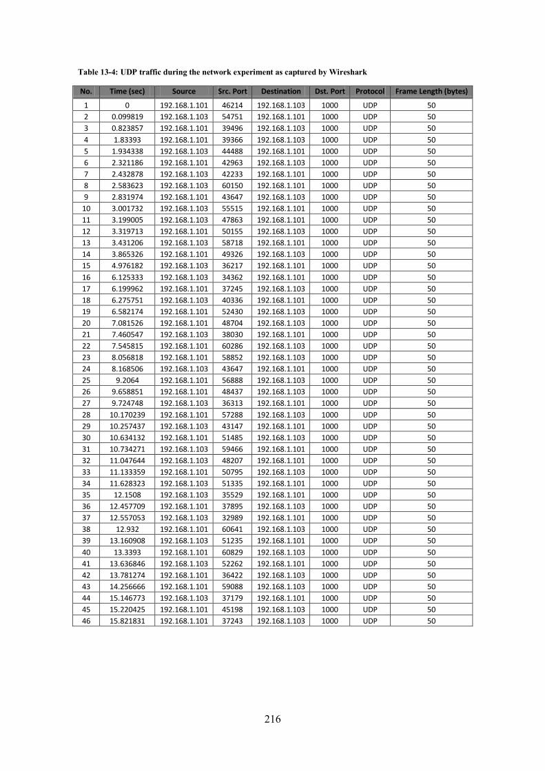
216
Table 13-4: UDP traffic during the network experiment as captured by Wireshark
No. Time (sec) Source Src. Port Destination Dst. Port Protocol Frame Length (bytes)
1 0 192.168.1.101 46214 192.168.1.103 1000 UDP 50
2 0.099819 192.168.1.103 54751 192.168.1.101 1000 UDP 50
3 0.823857 192.168.1.101 39496 192.168.1.103 1000 UDP 50
4 1.83393 192.168.1.101 39366 192.168.1.103 1000 UDP 50
5 1.934338 192.168.1.103 44488 192.168.1.101 1000 UDP 50
6 2.321186 192.168.1.101 42963 192.168.1.103 1000 UDP 50
7 2.432878 192.168.1.103 42233 192.168.1.101 1000 UDP 50
8 2.583623 192.168.1.103 60150 192.168.1.101 1000 UDP 50
9 2.831974 192.168.1.101 43647 192.168.1.103 1000 UDP 50
10 3.001732 192.168.1.103 55515 192.168.1.101 1000 UDP 50
11 3.199005 192.168.1.103 47863 192.168.1.101 1000 UDP 50
12 3.319713 192.168.1.101 50155 192.168.1.103 1000 UDP 50
13 3.431206 192.168.1.103 58718 192.168.1.101 1000 UDP 50
14 3.865326 192.168.1.101 49326 192.168.1.103 1000 UDP 50
15 4.976182 192.168.1.103 36217 192.168.1.101 1000 UDP 50
16 6.125333 192.168.1.103 34362 192.168.1.101 1000 UDP 50
17 6.199962 192.168.1.101 37245 192.168.1.103 1000 UDP 50
18 6.275751 192.168.1.103 40336 192.168.1.101 1000 UDP 50
19 6.582174 192.168.1.101 52430 192.168.1.103 1000 UDP 50
20 7.081526 192.168.1.101 48704 192.168.1.103 1000 UDP 50
21 7.460547 192.168.1.103 38030 192.168.1.101 1000 UDP 50
22 7.545815 192.168.1.101 60286 192.168.1.103 1000 UDP 50
23 8.056818 192.168.1.101 58852 192.168.1.103 1000 UDP 50
24 8.168506 192.168.1.103 43647 192.168.1.101 1000 UDP 50
25 9.2064 192.168.1.101 56888 192.168.1.103 1000 UDP 50
26 9.658851 192.168.1.101 48437 192.168.1.103 1000 UDP 50
27 9.724748 192.168.1.103 36313 192.168.1.101 1000 UDP 50
28 10.170239 192.168.1.101 57288 192.168.1.103 1000 UDP 50
29 10.257437 192.168.1.103 43147 192.168.1.101 1000 UDP 50
30 10.634132 192.168.1.101 51485 192.168.1.103 1000 UDP 50
31 10.734271 192.168.1.103 59466 192.168.1.101 1000 UDP 50
32 11.047644 192.168.1.103 48207 192.168.1.101 1000 UDP 50
33 11.133359 192.168.1.101 50795 192.168.1.103 1000 UDP 50
34 11.628323 192.168.1.103 51335 192.168.1.101 1000 UDP 50
35 12.1508 192.168.1.103 35529 192.168.1.101 1000 UDP 50
36 12.457709 192.168.1.101 37895 192.168.1.103 1000 UDP 50
37 12.557053 192.168.1.103 32989 192.168.1.101 1000 UDP 50
38 12.932 192.168.1.101 60641 192.168.1.103 1000 UDP 50
39 13.160908 192.168.1.103 51235 192.168.1.101 1000 UDP 50
40 13.3393 192.168.1.101 60829 192.168.1.103 1000 UDP 50
41 13.636846 192.168.1.103 52262 192.168.1.101 1000 UDP 50
42 13.781274 192.168.1.101 36422 192.168.1.103 1000 UDP 50
43 14.256666 192.168.1.101 59088 192.168.1.103 1000 UDP 50
44 15.146773 192.168.1.103 37179 192.168.1.101 1000 UDP 50
45 15.220425 192.168.1.101 45198 192.168.1.103 1000 UDP 50
46 15.821831 192.168.1.101 37243 192.168.1.103 1000 UDP 50
217
14 References
Akoumianakis, D. and C. Alexandraki. 2012. “Collective Practices in Common
Information Spaces: Insight from Two Case Studies,” Human-Computer
Interaction Journal. 27(4): 311-351.
Alexandraki C. and R. Bader. 2014. "Using computer accompaniment to assist
networked music performance," Proceedings of the AES 53rd Conference on
Semantic Audio, pp. 1-10. [Best Poster Award]
Alexandraki, C. and R. Bader. 2013. "Real-time concatenative synthesis for networked
musical interactions," Proceedings of Meetings on Acoustics, 19, art. no. 035040,
9 p.
Alexandraki, C. and D. Akoumianakis. 2010. “Exploring New Perspectives in Network
Music Performance: The DIAMOUSES Framework,” Computer Music Journal,
34(2): 66-83.
Alexandraki, C., Koutlemanis, P., Gasteratos, P., Valsamakis, N., Akoumianakis, D.,
Milolidakis, G., Vellis, G. and D. otsalis, D. 2008. “Towards the
Implementation of a Generic Platform for Networked Music Performance: The
DIAMOUSES approach,” Proceedings of the ICMC 2008 International Computer
Music Conference. pp. 251-258.
Alexandraki, C., and I. alantzis. 2007. “Requirements and Application Scenarios in
the Context of Network Based Music Collaboration,” Proceedings of the
AXMEDIS 2007 Conference. Florence: Firenze University Press, pp. 39–46.
Amado, R. G., and J. V. Filho. 2008. “Pitch detection algorithms based on zero-cross
rate and autocorrelation function for musical notes,” 2008 International
Conference on Audio Language and Image Processing, pp. 449-454.
Arom, S. 1991. African polyphony and polyrhythm: Musical structure and
methodology. Cambridge University Press.
Arulampalam, M. S., Maskell, S. and N. Gordon. 2002. “A tutorial on particle filters for
online nonlinear/non-gaussian bayesian tracking,” IEEE Transactions on Signal
Processing, 10(2): 174–188
Arzt, A., Widmer, G. and S. Dixon. 2008 “Automatic page turning for musicians via
real-time machine listening,” In Proceedings of the European Conference on
Artificial Intelligence, pp. 241–245.
Aucouturier, J.-J., and F. Pachet. 2006. "Jamming with Plunderphonics: Interactive
Concatenative Synthesis of Music" Journal of New Music Research 35(1): 35-50.
Bader R. 2013a. “Timbre.” In Nonlinearities and Synchronization in Musical Acoustics
and Music Psychology, edited by Rolf Bader, 329-379. Springer series on Current
Research in Systematic Musicology, Springer.
218
Bader R. 2013b. “Rhythm.” In Nonlinearities and Synchronization in Musical Acoustics
and Music Psychology, edited by Rolf Bader, 329-379. Springer series on Current
Research in Systematic Musicology, Springer.
Barbosa, A. 2006. “Computer-Supported Cooperative Work for Music Applications”.
PhD diss., Pompeu Fabra University, Barcelona, Spain
Barbosa, A. 2003. “Displaced Soundscapes: A Survey of Network Systems for Music
and Sonic Art Creation.,” Leonardo Music Journal 13:53–59.
Bárdi T. 2006. "High Resolution Speech F0 Modification," 3rd Speech Prosody Intl.
Conference
Barry, D., Dorran, D. and Coyle, E. 2008. “Time and pitch scale modification: a real-
time framework and tutorial,” Proceedings of the 11th. International Conference
on Digital Audio Effects (DAFx-08), pp. 103-110.
Baudoin, G. and El Chami F. 2003 “Corpus based very low bit rate speech coding.” In
Proceedings of the IEEE International Conference on Acoustics, Speech, and
Signal Processing, pp. 792-795.
Bello, J. P., Daudet, L., Abdallah, S., Duxbury, C., Davies, M. and M. B. Sandler. 2005.
“A Tutorial on Onset Detection in Music Signals,” IEEE Transactions On Speech
And Audio Processing, 13(5): 1035-1047.
Bello, J. P., and J. Pickens. 2005. “A Robust Mid-level Representation for Harmonic
Content in Music Signals.” In Proc ISMIR, ed. Joshua D Reiss and Geraint A
Wiggins, pp: 304-311.
Bello, J.P., Duxbury, C., Davies, M. and M. Sandler. 2004. “On the use of phase and
energy for musical onset detection in the complex domain,” IEEE Signal
Processing Letters, 4(6): 553–556.
Bello, J. P., and M Sandler. 2003. “Phase-based note onset detection for music signals.”
In Proc IEEE International Conference on Acoustics Speech and Signal
Processing (ICASSP 03), pp. 441-444.
Benetos, E., Dixon, S., Giannoulis, D., irchhoff, H. And lapuri, A. 2012. “Automatic
Music Transcription: Breaking the glass ceiling” In 13th International Conference
on Music Information Retrieval (ISMIR 2012), pp. 379-384.
Bi, C. 2009. “DNA motif alignment by evolving a population of Markov chains,” BMC
Bioinformatics 10, no. Suppl 1: S13.
Bilmes, Jeff A. 1998. “A Gentle Tutorial of the EM Algorithm and its Application to
Parameter Estimation for Gaussian Mixture and Hidden Markov Models,”
International Computer Science Institute 4, no. 510: 126.
Bischoff, J., Gold, R., and J. Horton. 1978. “Music for an Interactive Network of
Microcomputers,” Computer Music Journal, 2(3), 24–29
219
Bloch, J. B. and Dannenberg, R.B., 1985. “Real-Time Computer Accompaniment of
Keyboard Performances.” In Proceedings of the 1985 International Computer
Music Conference, International Computer Music Association, pp. 279-289
Bonada, J. And X. Serra. 2007. “Synthesis of the Singing Voice by Performance
Sampling and Spectral Models”, IEEE Signal Processing Magazine, 24(2): 67-79
Bonada , J., and A. Loscos. 2003. “Sample-Based Singing Voice Synthesis Based in
Spectral Concatenation.” Proceedings of the 2003 Stockholm Music and Acoustics
Conference. Stockholm: KTH, pp. 439–442.
Bharucha, J. J. And P. Todd.1989. “Modeling the perception of tonal structures with
neural nets,” Computer Music Journal 13: 44-53
Bregman, Albert S. 1990. Auditory Scene Analysis: The Perceptual Organization of
Sound. MIT Press.
Brossier, P. 2006. “Automatic annotation of musical audio for interactive applications.”
PhD diss., Queen Mary, University of London.
Brossier, P., Bello, J.P. and M.D Plumbley. 2004. ”Fast labelling of notes in music
signals,” In 5th International Conference on Music Information Retrieval (ISMIR-
04).
Buillot N. 2007. “nJam user experiments: enabling Remote Musical Interaction from
milliseconds to seconds.” In New Interfaces for Musical Expression (NIME'07),
6p.
Cabral, J. P. and Oliveira, L. C., "Pitch-Synchronous Time-Scaling for Prosodic and
Voice Quality Transformations", Proc. Interspeech'2005.
Cáceres, J. P., and C. Chafe. 2009. “JackTrip: Under the Hood of an Engine for
Network Audio.” Proceedings of the 2009 International Computer Music
Conference. San Francisco, California: International Computer Music
Association, pp. 509–512.
Cáceres, J.P. and A. Renaud. 2008. “Playing the network: the use of time delays as
musical devices.” In Proceedings of International Computer Music Conference,
pp. 244–250.
Cai, R., Lu, L., Hanjalic, A., Zhang H-J. and L-H Cai. 2006. “A flexible framework for
key audio effects detection and auditory context inference,” IEEE Transactions
on Audio Speech and Language Processing, 14(3):1026-1039.
Casey, M. A., Veltkamp, R., Goto, M., Leman, M., Rhodes, C. and M. Slaney. 2008.
“Content-Based Music Information Retrieval: Current Directions and Future
Challenges,” Proceedings of the IEEE, 96(4): 668-696.
Carôt, A., Rebelo, P. and A. Renaud. 2007. “Networked Music Performance: State of
the Art.” Proceedings of the AES 30th International Conference.
Saariselka, Finland: Audio Engineering Society. pp. 16-22.
Carôt, A., and C. Werner. 2007. “Network Music Performance—Problems, Approaches
and Perspectives.” Proceedings of the Music in the Global Village Conference.

220
Available online:
http://globalvillagemusic.net/2007/wp-content/uploads/carot_paper.pdf
Carôt, A., Renaud, A. and B. Verbrugghe. (2006) Network Music Performance (NMP)
with Soundjack, in Proceedings of the 6th NIME Conference, Paris, France, 2006
Carôt, A., rämer, U. and G. Schuller. 2006. “Network Music Performance (NMP) in
Narrow Band Networks,” Proceedings of the 120th AES convention.
Carvalho, P., Trancoso, I.M., and L.C. Oliveira. 1998. "Automatic Segment Alignment
for Concatenative Speech Synthesis in Portuguese", Proc. of the 10th
Portuguese
Conference on Pattern Recognition, RECPAD'98, pp. 221-226.
Cernocky, J., Baudoin, G., and G. Chollet, G. 1998. “Segmental Vocoder – Going
Beyond the Phonetic Approach.” IEEE ICASSP, pp. 605-608.
Chafe C. 2011. “Living with Net Lag,” In Proceedings of the 43rd AES International
Conference: Audio for Wirelessly Networked Personal Devices.
Chafe, C., Gurevich, M., Leslie, G. and S. Tyan. 2004. “Effect of Time Delay on
Ensemble Accuracy.” In Proceedings of the International Symposium on Musical
Acoustics.
Chafe, C. 2003. “Distributed Internet Reverberation for Audio Collaboration,”
Proceedings of the 24th
AES International Conference, pp. 13-19.
Chafe, C., Wilson, S., Leistikow, R., Chisholm, D. And G. Scavone. 2000. “A
Simplified Approach to High Quality Music and Sound Over IP.” Proc. COSTG6
Conference on Digital Audio Effects (DAFx-00).
Chafe, C., Mont-Reynaud, B. and L. Rush. 1982. “Toward an Intelligent Editor of
Digital Audio: Recognition of Musical Structures,” Computer Music Journal
6(1): 30-41.
de Cheveigné A. and H. awahara. 2002. “YIN, A Fundamental Frequency Estimator
for Speech and Music,” Journal of the Acoustical Society of America, vol. 111,
pp. 1917–1930.
Chew, E., Sawchuk, A. Tanoue, C. and R. Zimmermann. 2005. “Segmental Tempo
Analysis of Performances in User-Centered Experiments in the Distributed
Immersive Performance Project,” In Proceedings of the Sound and Music
Computing Conference, 12 p.
Cho, T. and J. P. Bello. 2008. “Real-time implementation of HMM-based chord
estimation in musical audio,” Proceedings of the International Computer Music
Conference ICMC, pp: 16–21.
Clarke, Eric F. 2001. Generative principles in music performance. In Generative
Processes in Music: The Psychology of Performance , Improvisation, and
Composition, ed. John Sloboda, 1-26. Oxford University Press.
Collier, G. L. And J. L. Collier. 2002. “A Study of Timing in two Louis Armstrong
Solos.“ In: Music Perception 19(3): 463-483.

221
Collins, N.S 2006. “Towards Autonomous Agents for Live Computer Music: Realtime
Machine Listening and Interactive Music Systems”, PhD diss., University of
Cambridge
Cont, A. 2010. “A Coupled Duration-Focused Architecture for Real-Time Music-to-
Score Alignment,” IEEE Transactions on Pattern Analysis and Machine
Intelligence, 32(6): 974-987.
Cont, A. 2008a. “ANTESCOFO: Anticipatory Synchronization and Control of
Interactive Parameters in Computer Music,” Proceedings of the International
Computer Music Conference.
Cont, A. 2008b. “Modeling Musical Anticipation: From the time of music to the music
of time” PhD thesis, University of Paris 6 and University of California in San
Diego
Cont A. 2004. “Improvement of Observation Modeling for Score Following.” IRCAM.
Available online: http://citeseerx.ist.psu.edu/viewdoc/download?doi=10.1.1.104.4970&rep=rep1&type=pdf
Cooperstock, J., and S. Spackman. 2001. “The Recording Studio that Spanned a
Continent.” In Proceedings of the International Conference on Web Delivering of
Music (WEDELMUSIC 2001). Florence, Italy:Wedelmusic, pp. 161–167.
de la Cuadra, P., Master, A. and C. Sapp. 2001. “Efficient Pitch Detection Techniques
for Interactive Music,” Proceedings of the International Computer Music
Conference, pp: 403–406.
Dannenberg R.B. 2012. “Human Computer Music Performance” . In Multimodal Music
Processing, edited by Müller M., Goto M., Schedl M., 121- 133, Wadern:
Dagstuhl - Leibniz Center for computer science GmbH.
Dannenberg, R.B. 2011. ”A Vision of Creative Computation in Music Performance,” in
Proceedings of the Second International Conference on Computational Creativity,
pp. 84-89.
Dannenberg, R. B, and C. Raphael. 2006. “Music score alignment and computer
accompaniment,” Communications of the ACM 49(8): 38.
Dannenberg R. 2006. “Concatenative Synthesis using Score-Aligned Transcriptions,”
Proceedings of the 2006 International Computer Music Conference, Computer
Music Association, pp. 352-355.
Dannenberg, R.. 2002. “Listening to “Naima”: An Automated Structural Analysis of
Music from Recorded Audio.” In Proceedings of the International Computer
Music Conference (ICMC), pp. 28-34.
Dannenberg, R., Sanchez, M., Joseph, A., Capell, P., Joseph, R. and R. Saul.1993. “A
computer-based multi-media tutor for beginning piano students,” Journal of New
Music Research, 19(2-3): 155–173
Dannenberg, R. B. 1989. “Real-Time Scheduling and Computer Accompaniment.” In
Mathews, M.and Pierce, J. eds. Current Research in Computer Music, MIT Press,
Cambridge, pp. 225-261.
222
Dannenberg R. 1984. “An On-Line Algorithm for Real-Time Accompaniment,”
Proceedings of the 1984 International Computer Music Conference, Computer
Music Association, pp. 193-198.
Dansereau, D.G., Brock, N. and J.R. Cooperstock. 2013. “Predicting an Orchestral
Conductor’s Baton Movements Using Machine Learning,” Computer Music
Journal, 37(2): 28-45
Daubechies, I., and W. Sweldens. 1998. “Factoring wavelet transforms into lifting
steps,” The Journal of Fourier Analysis and Applications 4(3): 247-269.
Delgado, M., Fajardo, W. and M. Molina-Solana. 2011. “A state of the art on
computational music performance,” Expert Systems with Applications 38(1): 155-
160.
Delignières, D., Lemoine, L. And K. Torre. 2004. “Time intervals production in tapping
and oscillatory motion,” Human Movement Science 23: 87–103
Dessein, A., Cont, A., and G. Lemaitre. 2010. “Real-time polyphonic music
transcription with non-negative matrix factorization and beta-divergence,”
In Proceedings of the 11th International Society for Music Information Retrieval
Conference (ISMIR), pp. 489–494.
Dixon, S. 2006. “Onset detection revisited.” In Proc of the Int Conf on Digital Audio
Effects DAFx06, pp. 133–137.
Dixon, S. 2005. “Live Tracking of Musical Performances using On-Line Time
Warping”, Proceedings of the 8th International Conference on Digital Audio
Effects (DAFx05), pp 92-97.
Dixon, S. and Widmer, G. 2005. “MATCH : A Music Alignment Tool Chest”, 6th
International Conference on Music Information Retrieval (ISMIR 2005).
Downie, J S. 2008. “The music information retrieval evaluation exchange (2005–2007):
A window into music information retrieval research,” Acoustical Science And
Technology, 29(4): 247-255.
Driessen, P. F., Darcie, T. E. And B. Pillay. 2011. “The Effects of Network Delay on
Tempo in Musical Performance.” Computer Music Joural, 35(1): 76-89
Duan Z. and B. Pardo. 2011a. “A state space model for online polyphonic audio-score
alignment,” Proceedings of IEEE ICASSP 2011, pp. 197-200.
Duan, Z. and B. Pardo. 2011b. “Soundprism: an online system for score-informed
source separation of music audio,” IEEE Journal of Selected Topics in Signal
Process., 5(6): 1205-1215.
Duan, Z., Pardo B. and C. Zhang. 2010. “Multiple fundamental frequency estimation
by modeling spectral peaks and non-peak regions,” IEEE Trans. Audio Speech
Language Process., 18(8): 2121-2133
Dutoit T. 2008. “Corpus-based Speech Synthesis.” In Springer Handbook of Speech
Processing edited by Benesty Jacob, Sondhi, M. M. and Huang, Yiteng, 437-453.
Springer: Springer Handbooks.
223
Dutoit T. 1996. An Introduction to Text-to-Speech Synthesis. Dordrecht: Kluwer
Academic Publishers.
Duxbury, C., Davies, M. and M. Sandler. 2003. “Complex domain onset detection for
musical signals,” In Proceedings of the International Conference on Digital Audio
Effects (DAFx-03), pp. 90–93.
Duxbury, C, Sandler, M, and M Davies. 2002a. “A hybrid approach to musical note
onset detection,” In Proc. of the 5th Int. Conference on Digital Audio Effects
(DAFx-02), pp. 33-38.
Duxbury, C., Davies, M. and M. Sandler. 2002b. “Improved time-scaling of musical
audio using phase locking at transients”. In Proceedings of the 112th AES
Convention. Paper 5530.
Duxbury, C., Davies, M. and M. Sandler. 2001. “Separation of transient information in
musical audio using multiresolution analysis techniques.” In Proceedings of the
COST G-6 Conference on Digital Audio Effects (DAFX-01), pp. 6-9.
Eggink J. and G.J. Brown. 2003. “A missing feature approach to instrument
identification in polyphonic music.” In ICASSP, volume 5, pp. 553–556, 2003.
Ellis, M. 1991. “An Analysis of 'Swing' Subdivisions and Asynchronization in Three
Jazz Saxophonists.” In: Perceptual and Motor Skills, 73(3): 707-713.
Fagerlönn, J, and H Alm. 2010. Auditory signs to support traffic awareness. IET
Intelligent Transport Systems, 4(4), 262
Fechner, G T. 1860. Elemente der Psychophysik. Ed. H E Adler, D H Howes, and E G
Boring. Search. Vol. 3. Breitkopf und Härtel.
Fink, G.A. 2008. “Configuration oh Hidden Markov Models.” In Markov Models for
Pattern Recognition, 127-136, Springer.
Flanagan J.L. and R. M. Golden. 1966. ‘Phase vocoder’. Bell System Technical Journal,
vol. 45, pp. 1493-1509.
Flexer A. 2006. “Statistical Evaluation of Music Information Retrieval Experiements,”
Journal of New Music Research, 35(2): 113-120
Follmer, G. 2005. “Electronic, Aesthetic and Social Factors in Net Music,” Organised
Sound, 10(3):185–192.
Folio C. and R.W. Weisberg. 2006. "Billie Holiday's Art of Paraphrase: A Study in
Consistency," In: New Musicology, Poland: Poznan Press, pp. 249-277.
Forney G.T. 1973. “The Viterbi algorithm,” Proc IEEE, vol. 61, pp. 268-178.
Fracile, N. 2003. "The 'Aksak' Rhythm, a Distinctive Feature of the Balkan Folklore".
Studia Musicologica Academiae Scientiarum Hungaricae 44 (1 and 2):197–210
Friberg, A. and A. Sundström. 2002. “Swing Ratios and Ensemble Timing in Jazz
Performacne: Evidence for a Common Rhythmic Pattern.” In: Music Perception
19(3): 333-49.
224
Friberg, A., Bresin, R. and L. Frydén. 1998. “Musical Punctuation on the Microlevel:
Automatic Identification and Performance of Small Melodic Units.” Journal of
New Music Research 27(3):217–292
Friston, arl J. 2010. “The free-energy principle: a unified brain theory?” Nature
Reviews Neuroscience 11: 127-138
Friston, K.J., Daunizeau, J., Kilner, J., and S.J. Kiebel. 2010. “Action and behaviour: a
free-energy formulation,” Biological Cybernetics 102: 227-260
Fritsch, J. 2012. “High Quality Musical Audio Source Separation.” Master’sthesis,
UPMC / IRCAM / Telecom Paristech.
Fu, L., Mao, X. and L. Chen. 2008. “Speaker independent emotion recognition based
on SVM/HMMS fusion system,” Audio Language and Image Processing 2008
ICALIP 2008 International Conference on, pp. 61–65.
Fu, Z., Lu, G., Ting, . and D. Zhang, D. 2011.”A survey of audio-based music
classification and annotation,” IEEE Transactions on Multimedia, 2(13): 303-319.
Gabrielsson, A. and E. Lindström. 2010. “The role of structure in musical expression of
emotions.” In: Sloboda, John A. & Juslin, Patrik N. (eds.): Handbook of Music
and Emotion. Theory, Research, Applications. Oxford University Press, pp. 367-
395.
Gabrielsson, A. 1999. “The performance of music.” In D.Deutsch (Ed.), The
Psychology of Music (2nd ed.), pp. 501-602. San Diego, CA: Academic Press.
Gabrielsson, A. 1982. “Perception and Performance of Musical Rhythm.” In: Manfred
Clynes (ed): Music, Mind and the Brain: The Neurophsychology of Music. NY,
Plenum Press, 159-169.
Garner, W. R. 1974. The processing of information and structure. Wiley & Sons, 1974.
Gibson D.B. 2014. “Challenges in Speech Coding.” In Speech and Audio Processing for
Coding, Enhancement and Recognition, edited by Tokunbo Ogunfunmi, Roberto
Togneri and Madihally Narasimha, Springer.
Gilden, D.L. 2001. “Cognitive Emissions of 1/f Noise,” Psychological Review 108(1):
33–56
Gjerdingen, R.O. 1990. “Categorization of musical patterns by self-organizing
neuronlike networks,” Music Perception 8: 339-370
Glover, J, Lazzarini, V. And J. Timoney. 2011. “Real-time detection of musical onsets
with linear prediction and sinusoidal modelling,” EURASIP Journal of advances
in Signal Processing, 60(1):1-13.
Goebl, W. and C. Palmer. 2009. “Synchronization of timing and motion among
performing musicians,” Music Perception, 26(5):427–438.
Goldstein, J L. 1973. “An optimum processor theory for the central formation of the
pitch of complex tones,” Journal of the Acoustical Society of America 54(6):
1496-1516.
225
Goldstein, J L. 1973. “An optimum processor theory for the central formation of the
pitch of complex tones,” Journal of the Acoustical Society of America 54(6):
1496-1516.
Gordon, J W. 1987. “The perceptual attack time of musical tones.” Journal of the
Acoustical Society of America 82(1): 88-105.
Goto, M. 2001a. “An Audio-based Real-time Beat Tracking System for Music With or
Without Drum-sounds,” Journal of New Music Research 30(2): 159-171
Goto, M. 2001b. “A predominant-f0 estimation method for real-world musical audio
signals: MAP estimation for incorporating prior knowledge about f0s and tone
models,” In Proc Workshop on Consistent and reliable acoustic cues for sound, 1-
4
Goto, M., Neyama, R., and Y. Muraoka. 1997. “RMCP: Remote Music Control
Protocol – design and Interactive Network Performance applications,” Proc. of the
1997 Int. Computer Music Conf. Thessaloniki, Hellas: ICMA, pp. 446–449.
Gotzen, A., Bernardini, N. and D. Arfib. 2000. “Traditional (?) implementations of a
phase vocoder: the tricks of the trade.” In Proceedings of the International
Conference on Digital Audio Effects (DAFx-00), pp. 37–44.
Grey, J M. 1977. “Multidimensional perceptual scaling of musical timbres,” Journal of
the Acoustical Society of America 61(5): 1270-1277.
Grachten, M. and Widmer G. 2012. “Linear Basis Models for Prediction and Analysis
of Musical Expression,” Journal of New Music Research 41(4): 311-322
Grubb, L. And R. Dannenberg. 1998. “Enhanced Vocal Performance Tracking Using
Multiple Information Sources”, Proceedings of the ICMC 1998 International
Computer Music Conference. pp. 37-44.
Gu, X., Dick, M., Kurtisi, Z., Noyer, U. and L. Wolf. 2005. "Network-centric Music
Performance: Practice and Experiments," IEEE Communications Magazine,
43(6): 86-93.
Hadjakos, A., Aitenbichler, E. and M. Mühlhäuser. 2008. "Parameter Controlled
Remote Performance (PCRP): Playing Together Despite High Delay". In
Proceedings of the 2008 International Computer Music Conference (ICMC), pp.
259-264.
Hainsworth S. and M. Macleod. 2003. “Onset detection in music audio signals,” In
Proceedings of the International Computer Music Conference (ICMC), pp. 163-
166.
Hajdu, G. 2006. “Automatic Composition and Notation in Network Music
Environments.” Proceedings of the 2006 Sound and Music Computing
Conference. Marseille: Centre National de Creation Musicale, pp. 109–114.
Hajdu, G. 2005. “Quintet.net: An Environment for Composing and Performing Music
on the Internet.” Leonardo Music Journal 38(1):23–30
226
Haken, H., Kelso, J.A.S. and H. Bunz, H. 1985. “A theoretical model of phase
transitions in human hand movements,” Biological Cybernetics 51: 347–356
Hansen, Mark M. B. 2006. New Philosophy for New Media. Cambridge: MIT Press.
Harma, A., Mc inney, M. F. and J. Skowronek. 2005. “Automatic surveillance of the
acoustic activity in our living environment,” in IEEE Int. Conf. Multimedia and
Expo, Amsterdam, The Netherlands, Jul. 2005.
Hasegawa-Johnson M. Alwan A. 2003. “Speech Codding: Fundamental and
Applications” In Wiley Encyclopedia of Telecommunications, edited by John G.
Proakis, John Wiley & Sons, Inc.
Hatlevik, E. 2012. “Are Musicians Affected by Room Acoustics in Rehearsal Rooms?”,
Master Thesis, Norwegian University of Science and Technology.
Hedfors, P., Grahn, P., Schafer, R. and H. Jarviluoma, Eds. 1998. “Soundscapes in
urban and rural planning and design—A brief communication of a research
project,” in Northern Soundscapes: Yearbook of Soundscape Studies, vol. 1, pp.
67–82.
Hiraga, R., Bresin, R., Hirata, ., and atayose, H. 2004. “Rencon 2004: Turing test for
musical expression,” In Proceedings of the 2004 conference on new interfaces for
musical expression (NIME04), pp. 120–123.
Hu, N., Dannenberg, R. B. and G Tzanetakis. 2003. “Polyphonic audio matching and
alignment for music retrieval.” In 2003 IEEE Workshop on Applications of Signal
Processing to Audio and Acoustics, pp. 185-188.
IETF (Internet Engineering Task Force). 2012. “RFC 6716: Definition of the Opus
Codec”. Available at: http://tools.ietf.org/html/rfc6716 (Last visit: 11/1/2014).s
Jensen, J. 2009. Feature Extraction for Music Information Retrieval, PhD dissertation,
Aalborg, Denmark, Aalborg University.
Jensen, . 2007. “Multiple scale music segmentation using rhythm, timbre, and
harmony,” EURASIP Journal on Advances on Signal Processing, 2007(1): 159-
170.
Kapur, A., Wang, G. and P. Cook. 2005. “Interactive Network Performance: a dream
worth dreaming?,” Organised Sound 10(3): 209-219.
atayose, H. Hashida, M. De Poli, G. and . Hirata. 2012 “On Evaluating Systems for
Generating Expressive Music Performance: the Rencon Experience,” Journal of
New Music Reserach 41(4): 299-310.
Kalkandjiev, Z. S. and S. Weinzierl. 2013. “Room acoustics viewed from the stage:
Solo performers' adjustments to the acoustical environment,“ Proceedings of the
International Symposium on Room Acoustics, p. 10
Keil, C. and S. Feld. 1994. Music Grooves. Essays and Dialogues. University of
Chicago Press.
227
eller P. 2007. “Musical Ensemble Synchronisation,” In Proceedings of the
International Conference on Music Communication Science, pp. 80-83.
hreich, W., Granger, E., Miri, A. and R. Sabourin. 2010. “On the memory complexity
of the forward-backward algorithm,” Pattern Recognition Letters, 31: 91-99.
iranyaz, S., Qureshi, A.F. and M. Gabbouj. 2006. “A generic audio classification and
segmentation approach for multimedia indexing and retrieval,” IEEE
Transactions on Audio, Speech, and Language Processing, 14 (3): 1062–1081.
Klapuri, A, and M Davy. 2006. Signal Processing Methods for Music Transcription.
Ed. Anssi Klapuri and Manuel Davy. Signal Processing. Springer-Verlag New
York Inc.
Klapuri A. 2004. Signal Processing Methods for the Automatic Transcription of Music.
PhD Dissertation, Tampere University of Technology.
lapuri, A. 1999. “Sound onset detection by applying psychoacoustic knowledge.”
1999 IEEE International Conference on Acoustics Speech and Signal Processing
Proceedings ICASSP99 Cat No99CH36258 6, pp. 3089-3092.
von dem nesebeck, A., Ziraksaz, P. and U. Zölzer. 2010. “High quality time-domain
pitch shifting using PSOLA and transient preservation,” in Proc. 129th Audio
Eng. Soc. Convention, paper 8202.
Kostek, B. 2005. Perception-based data processing in acoustics. Applications to Music
Information Retrieval and Psychophysiology of Hearing. Springer.
raemer, U., Hirschfeld, J., Schuller, G., Wabnik, S., Carôt, A. And C. Werner. 2007.
“Network Music Performance with Ultra-Low-Delay Audio Coding under
Unreliable Network Conditions.” Proceedings of the 123rd Audio Engineering
Society Convention. New York: Curran Associates, pp. 338–348.
umar, R. S., Tamrakar N. and P. Rao.2008. “Segment based MBE speech coding at
1000 bps,” Proc. of National Conference on Communications (NCC).
Kuo, S.M., Lee, B.H. and W. Tian. 2006. “Introduction to Real-time Digital Signal
Processing.” In Real-Time Digital Signal Processing: Implementations and
Applications, edited by Kuo, S.M., Lee, B.H. and W. Tian, 1-48, John Wiley &
Sons, Ltd
urtisi, Z., and L. Wolf. 2008. “Using WavPack for Real-time Audio Coding in
Interactive Applications.” Proceedings of the 2008 International Conference on
Multimedia & Expo (IEEE ICME 2008). Hannover: IEEE Publishing, pp. 1381–
1384.
urtisi, Z., Gu, X. and L. C. Wolf 2006. “Enabling network-centric music performance
in wide-area networks,” ACM Communications Mag. 49(11): 52-54.
Langner J. and W. Goebl. 2003. “Visualizing expressive performance in tempo-
loudness space.” Computer Music Journal, 27(4): 69–83
228
Large, E. W. and C. Palmer. 2002. “Perceiving temporal regularity in music,” Cognitive
Science 26: 1 – 37
Laroche, J. 2003. “Frequency-Domain Techniques for High-Quality Voice
Modification.” Proceedings of the 2003 DAFx (Digital Audio Effects) Conference.
London: Queen Mary, University of London, pp. 328–332.
Laroche, J. 2002. “Time and pitch scale modification of audio signals,” in Applications
of Digital Signal Processing to Audio and Acoustics, M. Kahrs and K.
Brandenburg, Eds. Kluwer Academic Publishers.
Laroche, J.; “Dolson, M. 1999 “Improved phase vocoder. Time-Scale Modification of
Audio”, In IEEE Transactions on Speech and Audio Processing, 7(3): 323 –332.
Lazier, A. And P. Cook. 2003. “MOSIEVIUS: feature driven interactive audio
mosaicing,” Proc. of the 6th Int. Conference on Digital Audio Effects (DAFx-03)
Lazzaro, J., and J. Wawrzynek. 2001. “A Case for Network Musical Performance.”
Proceedings of ACM NOSSDAV [International Workshop on Network and
Operating Systems Support for Digital Audio and Video] 01. Port Jefferson, New
York: Association for Computing Machinery, pp. 157–166.
Lee M. E. and M. J. T. Smith 2002. “Digital Voice Synthesis using a new alternating
reflection Model,” IEEE International Symposium on Circuits and Systems,
IEEE-ISCAS 2002, pp. 863-866.
Leman, M. and F. Carreras. 1997. “Schema and Gestalt: Testing the hypothesis of
Psychoneural Isomorphism by Computer Simulation.” In: Marc Leman (ed.):
Music, Gestalt, and Computing. Studies in Cognitive and Systematic Musicology,
144-168. . Springer, Berlin.
Lerdahl, F. and R. Jackendoff. 1983. A Generative Theory of Tonal Music, Cambridge,
Mass.: MIT Press.
Lim, A., Mizumoto, T., Cahier, L., Otsuka, T., Takahashi, T., Komatani, K., Ogata,
K. and H. Okuno. 2010. "Robot musical accompaniment: integrating audio and
visual cues for real-time synchronization with a human flutist," In Intelligent
Robots and Systems (IROS), 2010 IEEE/RSJ International Conference on. IEEE,
pp. 1964-1969.
Lindemann, E. 2007. “Music Synthesis with Reconstructive Phrase Modeling.” IEEE
Signal Processing Magazine, 24(2): 80-91
Litovsky, R.Y., Colburn, H.S., Yost, W.A., and S. J. Guzman. 1999. "The precedence
effect". The Journal of the Acoustical Society of America 106: 1633–16.
Liu, Y., Dannenberg, R. and L Cai. 2010. “The Intelligent Music Editor: Towards an
Automated Platform for Music Analysis and Editing,” In Advanced Intelligent
Computing Theories and Applications With Aspects of Artificial Intelligence,
editied by Huang, D.-S.; Zhang, X.; Reyes Garcia, C.A.; Zhang, L., Springer:
Lecture Notes on Artificial Intelligence, Vol: 6216, pp.:123-131.
229
Maddox R. . and Larson, E. 2005. “Real-time time-domain pitch tracking using
wavelets,”
http://courses.physics.illinois.edu/phys406/NSF_REU_Reports/2005_reu/ Real-
Time_Time-Domain_Pitch_Tracking_Using_Wavelets.pdf (Last viewed 21 Apr.
2013)
Maestre, E., Ramírez, R., ersten, S., and X. Serra 2009. “Expressive Concatenative
Synthesis by Reusing Samples from Real Performance Recordings.” Computer
Music Journal, 33(4): 23-42.
Maia, R., Toda, T., Zen, H., Nankaku, Y. and K Tokuda. 2007. An excitation model for
HMM-based speech synthesis based on residual modeling. In ISCA SSW,
6(2):131-136.
Mäki-Patola T. 2005. “Musical Effects Of Latency.” Swomen Musiikintutkijoiden 9:82–
85.
Mäki-Patola, T. and P. Hämäläinen. 2004. “Effect of Latency on Playing Accuracy of
two Gesture Controlled Continuous Sound Instruments Without Tactile
Feedback.” Proceedings of the 7th International Conference on Digital Audio
Effects (DAFx'04), pp. 11-16.
Mann, T. P. 2006. “Numerically Stable Hidden Markov Model Implementation,”
Available online at:
http://bozeman.genome.washington.edu/compbio/mbt599_2006/hmm_scaling_rev
ised.pd (Last visit: 26/4/2013)
Marcae, R. and S. Dixon. 2010a. “Accurate Real-time Windowed Time Warping,” 11th
International Society for Music Information Retrieval Conference (ISMIR 2010),
pp. 423-428.
Macrae, R, and S Dixon. 2010b. “A guitar tablature score follower.” IEEE
International Conference on Multimedia and Expo ICME 2010, pp. 725-726.
Marchini , M. Papiotis, P. And E. Maestre. 2012. “Timing synchronization in string
quartet performance: a preliminary study,” In Proceedings of the International
Symposium on Computer Music Modelling and Retrieval (CMMR2012), pp. 177-
185.
Masri, P., Bateman, A., 1996. “Improved Modelling of Attack Transients in Music
Analysis-Resynthesis”, Proc.International Computer Music Conference
(ICMC96), pp. 100 – 103.
Mathews, M. 1991. “The Radio Baton and Conductor program, or: Pith, the most
important and least expressive part of music,” Computer Music Journal, 15(4):
37-46.
Mathews, M. 1989. “The Radio Drum as a synthesizer controller,” In Proc. Int.
Computer Music Conference, pp. 42-45.
Mcennis, D., C. Mckay, I. Fujinaga, and P. Depalle (2005). “jAudio: An feature
extraction library.” In 6th International Conference on Music Information
Retrieval (ISMIR).
230
Mendonça, David, and William A. Wallace. 2004. “Cognition in Jazz Improvisation:
An Exploratory Study.” In 26th Annual Meeting of the Cognitive Science Society,
pp. 1-6.
Meyer, L. B. 1956. Musical meaning and emotion in music. University of Chicago
Press.
Miklós, István, and Irmtraud M Meyer. 2005. “A linear memory algorithm for Baum-
Welch training,” BMC Bioinformatics 6, no. 1471-2105: 231.
Miotto, R. and Lanckriet, G. 2012. “A Generative Context Model for Semantic Music
Annotation and Retrieval,” IEEE Transactions on Audio, Speech and Language
Processing, 20(4): 1096-1108
Mizumoto, T., Hiroshi, T., Takahashi, T., Ogata, T. and H. Okuno. 2009. "Thereminist
robot: Development of a robot theremin player with feedforward and feedback
arm control based on a theremin's pitch model," in Intelligent Robots and Systems
(IROS), 2009 IEEE/RSJ International Conference on. IEEE, pp. 2297-2302.
Montecchio, N. and A. Cont. 2011a. “A unified approach to real time audio-to-score
and audio-to-audio alignment using sequential Montecarlo inference techniques,”
Proceedings of the IEEE International Conference on Acoustics, Speech, and
Signal Processing, pp. 193-196
Montecchio, N., and A. Cont. 2011b. “Accelerating the Mixing Phase in Studio
Recording Productions by Automatic Audio Alignment,” 12th International
Society for Music Information Retrieval Conference (ISMIR 2011), pp. 627–632.
Moore, Brian C J. 2003. An Introduction to the Psychology of Hearing. Boston
Academic Press. Vol. 3. Academic Press.
Moorer J. A. 1975. “On the segmentation and analysis of continuous musical sound
bysigitl Computer.” PhD Dissertation, Stanford University.
Moulines, E. and F. Charpentier. 1990. “Pitch-synchronous waveform processing
techniques for text-to-speech synthesis using diphones,” Speech Communications,
9 (5-6): 453-467.
Müller, M. 2010. “Dynamic Time Warping.” In Information Retrieval for Music and
Motion, edited by Meinard Müller, 69-84, Springer
Müller, M. and D. Appelt. 2008. “Path-constrained partial music synchronization,”
Proceedings of the 34th International Conference on Acoustics, Speech and
Signal Processing (ICASSP), vol. 1, Las Vegas, Nevada, USA, pp. 65-68.
Müller, M., Mattes, H. and F. urth. 2006. “An efficient multiscale approach to audio
synchronization,” Proceedings of the 7th International Conference on Music
Information Retrieval (ISMIR), Victoria, Canada, pp. 192-197.
Narmour, E. 1990. The Analysis and Cognition of Basic Melodic Structures: The
Implication Realization Model. Chicago, Illinois: University of Chicago Press.
231
Nathan, K., Senior, A. and J. Subrahmonia. 1996. “Initialization of hidden Markov
models for unconstrained on-line handwriting recognition,” In Proceedings of
IEEE International Conference on Acoustics, Speech, and Signal Processing,
ICASSP-96, vol.6, pp: 3502-3505.
Niedermayer, B. 2009. “Improving Accuracy of Polyphonic Music-To-Score
Alignment,” Proceedings of the 10th International Society for Music Information
Retrieval Conference (ISMIR 2009), pp: 585-590.
Oliveira, A. P., and A. Cardoso. 2010. “A musical system for emotional expression,”
Knowledge-Based Systems 23(8): 901-913.
Orio, N. and F. Déchelle. 2001. “Score Following Using Spectral Analysis and Hidden
Markov Models,” In Proceedings of the International Computer Music
Conference ICMC, 27:1708-1710.
Orio, N. and D. Schwarz. 2001. “Alignment of monophonic and polyphonic music to a
score,” In Proceedings of the International Computer Music Conference.
Otsuka, T., Nakadai, K., Takahashi, T., Ogata, T. and H.G. Okuno. 2011. “Real-Time
Audio-to-Score Alignment Using Particle Filter for Coplayer Music
Robots,” EURASIP Journal on Advances in Signal Processing, 2011: 384651
doi:10.1155/2011/384651
Pachet, F. 1999. “Music listening: What is in the air?” Sony Computer Science
Laboratory internal Report.
Page, M. A. 1994. “Modeling the perception of musical sequences with self-organizing
neural networks,” Connection Science 6: 223-246
Park, S-H, Ju-Hong Lee, Jae-Won Song, and T-S Park. 2009. “Forecasting Change
Directions for Financial Time Series Using Hidden Markov Model,” Change,
5589 {LNAI, 184-191.
Pisczcalski M. and B. Geller. 1977. “Automatic Music Transcription,” Computer Music
Journal, 1(4): 24-31
Polycom. 2011. “Music Performance and Instruction over High-Speed Networks,” A
Polycom WhitePaper. Electronically available at: http://docs.polycom.com/global/documents/whitepapers/music_performance_and_instruction_over
_highspeed_networks.pdf
Pressing, J. 1999. “Sources of 1/f noise eff ects in human cognition and performance,” Paideusis, 2: 42–59
Pressing, J. 1988. “Improvisation: Methods and Models.” In Generative Processes in
Music, edited by John Sloboda, 129-178, Clarendon, Oxford.
Pritchett, J. (1993). The Music Of John Cage. Cambridge University Press, Cambridge,
UK.
Prögler, J.A. 1995. “Searching for Swing: Participatory Discrepeancies in the Jazz
Rhythm Section.” In Ethnomusicology 39(1): 21-54.
232
Rabiner L. R. and B. H. Juang 1993. Fundamentals of Speech Recognition, Prentice
Hall Signal Processing Series.
Rabiner, L. R. 1989. “A tutorial on Hidden Markov Models and selected applications in
speech recognition,” Proceedings of the IEEE 77 (2): 257–285.
Radhakrishnan, R., Divakaran, A. and P. Smaragdis. 2005. “Audio analysis for
surveillance applications,” IEEE Workshop on Applications of Signal Processing
to Audio and Acoustics 2005, pp. 158-161
Ramírez, R., Maestre, E., Pertusa, A., Gómez, E., & Serra, X. 2007. Performance-based
interpreter identification in saxophone audio recordings. IEEE Transactions on
Circuits and Systems for Video Technology 17(3): 356–364.
Raphael, C. 2004. “A Hybrid Graphical Model for Aligning Polyphonic Audio with
Musical Scores”, in Proceedings of the International Conference on Music
Information Retrieval, pp. 387–94.
Raphael, C. 2003. “Orchestral Musical Accompaniment from Synthesized Audio,"
Proceedings of the International Computer Music Conference, Singapore.
Raphael, C. 2002. “Automatic Transcription of Piano Music,” In Proc ISMIR, ed.
Michael Fingerhut, 2:13–17. Ircam - Centre Pompidou.
Raphael, C. 2001a. “Music Plus One: A System for Expressive and Flexible Musical
Accompaniment,” In Proceedings of the International Computer Music
Conference, pp. 159-162.
Raphael, C. 2001b. “A Bayesian Network for Real-Time Musical Accompaniment.” In
Proceedings of Advanced in Neural Information Processing Systems, pp. 1433-
1440.
Raphael, C. 1999. “Automatic segmentation of acoustic musical signals using hidden
Markov models,” IEEE Transactions on Pattern Analysis and Machine
Intelligence, 21(4): 360-370
Rasch, R. A. 1988. “Timing and synchronization in ensemble performance.” In J. A.
Sloboda (Ed.), Generative processes in music: The psychology of performance,
improvisation and composition (pp. 70-90). Oxford: Clarendon Press.
Richard G. and C. d’Alessandro. 1996. “Analysis/Synthesis and Modification of the
Speech Aperiodic Component,” Speech Communication (19):221–244
Rosa, A.A., Andrade, A.O, Soares, A.B. and S.J. Nasuto. 2007. “On the initialization of
parameters of Hidden Markov Models,” Available online at:
http://www.biolab.eletrica.ufu.br/admin/downloads/AngelaCeel2007.pdf (Last
visit: 25/4/2013)
Rose, R.F. 1989. “An Analysis of Timing in Jazz Rhythm Section Performance.” PhD
diss., University of Texas, Austin.
Rouas, J L. 2007. “Automatic Prosodic Variations Modeling for Language and Dialect
Discrimination,” IEEE Transactions On Audio Speech And Language Processing,
15(6): 1904-1911.
233
Roucos S. and A. Wilgus. 1985. “High quality time-scale modification for speech,” In
Proceedings of the IEEE International Conference on Acoustics, Speech, and
Signal Processing, pp: 493–496.
Roucos, S., Wilgus, A. and W. Russell. 1987. “A Segment Vocoder Algorithm for
Real-Time Implementation,” In Proceedings of the IEEE International
Conference on Acoustics, Speech, and Signal Processing, pp. 1949-1952.
Rowe, R. 2001. Machine Musicianship. Cambridge, MA: The MIT Press
Rowe, R. 1992. Interactive Music Systems: Machine Listening and Composing.
Cambridge, MA: The MIT Press
Sanderson, P., Crawford, J., Savill, A., Watson, M. And W.J. Russell, W.J. 2004.
“Visual and auditory attention in patient monitoring: a formative analysis,”
Cognition, Technology & Work 2004(6): 172-185.
Sarkar, M., and B. Vercoe. 2007. “Recognition and prediction in a network music
performance system for Indian percussion,” Proceedings of the 7th international
conference on New interfaces for musical expression NIME 07, pp. 317-320.
Sawchuk, A. A., Chew, E., Zimmermann, R., Papadopoulos, C. and C. Kyriakakis.
2003. “From Remote Media Immersion to Distributed Immersive Performance,”
Proceedings of the ACM SIGMM 2003. Workshop on Experiential Telepresence.
New York: ACM Press, pp. 110–120.
Schaeffer, P. 1966. “Traité des Objets Musicaux.” Editions Du Seuil.
Scharenborg, O. 2007. “Reaching over the gap: A review of efforts to link human and
automatic speech recognition research,” Speech Communication 49(5): 336-347.
Schedl, M., Widmer, G., nees, P. and T. Pohle. 2011. “A music information system
automatically generated via Web content mining techniques,” Information
Processing & Management 47(3): 426-439.
Schnell, N., Peeters, G., Lemouton, S. and X Rodet. 2000. “Synthesizing a choir in real-
time using Pitch Synchronous Overlap Add,” Proceedings of the International
Computer Music Conference
Schroeder M. R. and B. S. Atal. 1985. "Code-excited linear prediction (CELP): high-
quality speech at very low bit rates," in Proceedings of the IEEE International
Conference on Acoustics, Speech, and Signal Processing (ICASSP), vol. 10, pp.
937–940.
Schuett, N. 2002. “The effects of latency on ensemble performance.” Available online
at:https://ccrma.stanford.edu/groups/soundwire/publications/papers/schuett_honor
Thesis2002.pdf (Last visit: 25/6/2012)
Schwarz, D. 2007. Corpus-Based Concatenative Synthesis. (S.-F. Chang, Ed.) IEEE
Signal Processing Magazine, 24(2): 92-104.
Schwarz, D., Beller, G., Verbrugghe, B. and S. Britton. 2006. “Real-time corpus-based
concatenative synthesis with CataRT,” In Proc of the Int. Conf on Digital Audio
Effects DAFx06, pp: 279-282.
234
Schwarz, D. 2006. Concatenative Sound Synthesis: The Early Years. Journal of New
Music Research, 35(1), 3-22
Schwarz, D. 2004. “Data-Driven Concatenative Sound Synthesis.” PhD diss., Universite
Paris 6.
Schwarz, D. 2000a. “A system for data-driven concatenative sound synthesis,” In
Proceedings of COST-G6 Conference on Digital Audio Effects (DAFx) pp. 97 –
102.
Schwarz, D. 2000b. “A System for Data-Driven Concatenative Sound Synthesis,” In
Proc COST G6 Conf on Digital Audio Effects, pp. 97-102.
Scloss W.A. 1985. On the Automatic Transcription of Percussive Music - From
Acoustic Signal to High-Level Analysis. PhD Dissertation, Stanford University
Sheh and D. P.W. Ellis. 2003. “Chord segmentation and recognition using em-trained
hidden markov models,” In Proceedings of the 4th ISMIR, pp. 183–189.
Simon, I., Basu, S., Salesin, D., and M. Agrawala 2005. “Audio Analogies: Creating
new music from an existing performance by concatenative synthesis.”
Proceedings of the International Computer Music Conference ICMC’05.
Silla Jr., C. N., Koerich, A. L. and C. A. A. aestner. 2008. “A Machine Learning
Approach to Automatic Music Genre Classification,” Journal of the Brazilian
Computer Society, 14(3): 7–18.
Snyer, B. 2000. Music and memory. Cambridge University Press.
Soulez, F., Rodet, X. and D. Schwarz. 2003. “Improving Polyphonic and Poly-
Instrumental Music to Score Alignment.” Ed. Holger H Hoos and David
Bainbridge. International Conference on Music Information Retrieval (ISMIR),
pp: 143-148.
Spanias A. 1994. “Speech coding: A Tutorial Review,” Proceedings of the IEEE
82(10): 1541-1582
Srinivasan, S, and D Wang. 2005. “A schema-based model for phonemic
restoration,” Speech Communication, 45(1): 63-8
Srinivasan, A. 2012. “Speaker Identification and Verification using Vector Quantization
and Mel Frequency Cepstral Coefficients,” Engineering and Technology 4(1): 33-
40.
Steven, D. 1994. Musical Meaning and Expression. Ithaka: Cornell University Press.
Stowell, D. and M. Plumbley. 2007. “Adaptive whitening for improved real-time audio
onset detection.” Proceedings of the International Computer Music Conference
ICMC’07.
Stroppa, M. 1999. “Live electronics or live music? Towards a critique of interaction,”
Contemporary Music Review, 18(3):41–77.
235
Tanaka, A. 2006. “Interaction, Experience, and the Future of Music.” In . O’ Hara and
B. Brown, eds. Consuming Music Together: Social and Collaborative Aspects of Music
Consumption Technologies. Dordrecht, Netherlands: Springer, pp. 267–288.
Tatlas, N., Floros, A. Zarouchas, T. and John Mourjopoulos. 2007. “Perceptually-
Optimized Error Concealment for Audio Over WLANs.” The Mediterranean
Journal of Electronics and Communications 3(3): 77-86
Temperley, D. 2007. Music and Probability. The MIT Press.
Tetsuro, ., Goto, M., omatani, ., Ogata, T. and H.G Okuno. 2005. “Instrument
Identification in Polyphonic Music: Feature Weighting with Mixed Sounds, Pitch-
Dependent Timbre Modeling, and Use of Musical Context,” In Science And
Technology, ed. Joshua D Reiss and Geraint A Wiggins, 558-563.
Thompson, W. F., Schellenberg, E. G. and G. Husain. 2004. “Decoding speech prosody:
do music lessons help?” Emotion 4(1): 46-64.
Thornburg H. 2005. “Detection and Modeling of Transient Audio Signals With Prior
Information.” PhD diss., Stanford University.
Timmers, R. 2002. Freedom and constraints in timing and ornamentation:
investigations of music performance. Maastricht, Shaker.
Todd, N. P. 1992. The dynamics of dynamics: A model of musical expression. Journal
of the Acoustical Society of America 91(6): 3540-3550.
Toiviainen, P., Tervaniemi, M., Louhvuori, J., Saher, M., Huotilainen, M. and
Näätänen. 1998. “Timbre similarity: convergence of neural, behavioral, and
computational approaches,” Music Perception 16: 223-241
Tzanetakis G. and P. Cook. 2002. “Musical Genre Classification of Audio Signals,”
IEEE Transactions on Speech and Audio Processing, 10(5): 293-302.
Urbano J., Downie J., McFee B., Schedl M. 2012. “How Significant is Statistically
Significant? The Case of Audio Music Similarity and Retrieval,” in: Proceedings
of the 13th International Society for Music Information Retrieval Conference
(ISMIR 2012), 6p.
Valin, J. M., Maxwell, G., Vos, K. and T. B. Terriberry. 2013. “High-Quality, Low-
Delay Music Coding in the Opus Codec”, Proceedings of the 135th Audio
Engineering Society Convention, New York City.
Valin, J. M., Terriberry, T. B., Montgomery, C. and G. Maxwell. 2009. “A High-
Quality Speech and Audio Codec With Less Than 10 ms Delay.” IEEE
Transactions on Audio, Speech and Language Processing. 18(1): 58-67.
Vallis, O., Diakopoulos, D., Hochenbaum, J. And A. Kapur. 2012. “Building on the
Foundations of Network Music: Exploring Interaction Contexts and Shared
Robotic Instruments,” Organised Sound, 17(1):62-72
236
Vercoe, B. L., Gardner, W. G. and E. D. Scheirer. 1998. “Structured audio: Creation,
transmission, and rendering of parametric sound representations,” Proeedings of
IEEE, 86(3): 922–940.
Vercoe, B.L., and M.S. Puckette, (1985) “Synthetic Rehearsal: Training the Synthetic
Performer,” in Proceedings, ICMC, Burnaby, BC, Canada, pp. 275-278.
Vercoe, B.L. (1984) “The Synthetic Performer in the Context of Live Performance,” in
Proceedings, International Computer Music Conference, Paris, pp. 199-200.
Verhelst, W. and M. Roelands. 1993. “An Overlap-add Technique Based on Waveform
Similarity (WSOLA) for High Quality Time-Scale Modification of Speech,”
Proc. IEEE ICASSP-93, pp. 554–557.
Waadeland, C. H. 2001. “It Don't Mean a Thing If It Ain't Got That Swing: Simulation
Expressive timing Through Modulated Movements.” In Journal of New Music
Research 30(1), 23-37.
Wang, De L. 2007. “Computational scene analysis,” Challenges for computational
intelligence 191: 163-191.
Walker, W. F. 1997. “A Computer Participant in Musical Improvisation,” Proceedings
of the ACM Conference on Human Factors in Computing Systems (CHIʼ97), pp.
14-17.
Whalley I.2009. “Software Agents in Music and Sound Art Research/Creative Work:
current state and a possible direction,” Organised Sound, 14(2): 156-167.
Wichern, G., Jiachen, X., Thornburg H., Mechtley, B. and A Spanias. 2010.
“Segmentation, Indexing, and Retrieval for Environmental and Natural
Sounds,” IEEE Transactions On Audio Speech And Language Processing, 18(3):
688-707.
Widmer, G. and W. Goebl. 2004. “Computational models of expressive music
performance: The state of the art,” Journal of New Music Research, 33(3):203–
216.
Widmer, G. 2003. “Discovering simple rules in complex data: A meta-learning
algorithm and some surprising musical discoveries,” Artificial Intelligence 146(2):
129–148
Wing, A.M. and A.B. ristofferson. 1973. “Response delays and the timing of discrete
motor responses,” Perception and Psychophysics 14: 5–12
Wright, M., and A. Freed. 1997. “Open Sound Control: a new protocol for
communicating with sound synthesizers,” Proc. of the 1997 Int. Computer Music
Conf. Thessaloniki, Hellas: ICMA, pp. 101–104.
Wu, X., Dhara, K.K. and V. rishnaswamy. 2007. “Enhancing Application-Layer
Multicast for P2P Conferencing,” In Proceedings of the 4th
IEEE Consumer
Communications and Networking Conference, pp. 986-990.
237
Xiao, J., Tammam, T., Chunyu, L., and Yao Zhao. 2011. “Real-time forward error
correction for video transmission,” 2011 Visual Communications and Image
Processing (VCIP). IEEE.
Xiong, B. and O. Izmirli. 2012. “Audio-To-Audio Alignment Using Particle Filters to
Handle Small and Large Scale Performance Discrepancies,” Proceedings of the
International Computer Music Conference, pp. 539-542.
Xu, A., Woszczyk, W., Settel, Z., Pennycook, B., Rowe, R., Galanter, P., Bary, J.,
Martin, G., Corey, J., and J. Cooperstock. 2000. “Real time streaming of multi-
channel audio data through the Internet,” Journal of the Audio Engineering
Society, 48(7/8): 627-641.
Yadollahi, A., and Z. M. . Moussavi. 2006. “A robust method for heart sounds
localization using lung sounds entropy,” IEEE Transactions on Biomedical
Engineering, 53(3): 497-502.
Young, M. W. 2010. “Identity and Intimacy in Human-Computer Improvisation.”
Leonardo Music Journal, 20: 97-103
Zanon, P. and G. D. Poli. 2003. “Estimation of parameters in rule systems for
expressive rendering in musical performance,” Computer Music Journal 27(1):
29–46
Zatorre, R. J., J. L. Chen, and V. B. Penhune. 2007. “When the Brain Plays Music:
Auditory–Motor Interactions in Music Perception and Production.” Nature
Reviews Neuroscience, 8(7):547–558.
Zen, Heiga, eiichi Tokuda, and Alan W Black. 2009. “Statistical parametric speech
synthesis,” Speech Communication 51(11): 1039-1064.
Zils, A. and F. Pachet. 2001, "Musical Mosaicing", Proceedings of the COST G-6
Conference on Digital Audio Effects (DaFx-01), pp: 39–44.

238
Eidesstattliche Erklärung
Ich versichere an Eides Statt durch meine eigenhändige Unterschrift, dass ich die
beiliegende Arbeit selbstständig und ohne fremde Hilfe angefertigt und alle Stellen, die
wörtlich oder annähernd wörtlich aus Veröffentlichungen entnommen sind, als solche
kenntlich gemacht habe. Außerdem habe ich mich keiner anderen als der angegebenen
Literatur bedient. Diese Versicherung bezieht sich ebenfalls auf die dazu gehörigen
Zeichnungen, Skizzen und bildliche Darstellungen dieser Arbeit.
......................................... ...............................................................
Datum Chrisoula Alexandraki