realistic simulation and control of human swimming...
TRANSCRIPT
University of California
Los Angeles
Realistic Simulation and Control of Human
Swimming and Underwater Movement
A dissertation submitted in partial satisfaction
of the requirements for the degree
Doctor of Philosophy in Computer Science
by
Weiguang Si
2013

c© Copyright by
Weiguang Si
2013
Abstract of the Dissertation
Realistic Simulation and Control of Human
Swimming and Underwater Movement
by
Weiguang Si
Doctor of Philosophy in Computer Science
University of California, Los Angeles, 2013
Professor Demetri Terzopoulos, Chair
We present a multiphysics framework for the realistic animation of human swim-
ming that features a comprehensive biomechanical model of the human body
immersed in simulated fluid. Our human model includes all of the relevant
articular bones and muscles, including 103 bones (comprising 163 articular degrees
of freedom) plus a total of 823 muscle actuators embedded in a finite element
model of the the soft tissues of the body that produces realistic deformations. A
main focus of this thesis is the control of this complex biomechanical model. To
coordinate the numerous muscle actuators in order to produce natural swimming
movements, we develop a biomimetically motivated motor control system based on
Central Pattern Generators (CPG), which learns to produce activation signals that
drive the Hill-type muscle actuators. In addition, we introduce an optimization-
based control method that enables our human model to achieve non-locomotion,
task-oriented movements, such as changing the orientation of the body in the
water.
ii
The dissertation of Weiguang Si is approved.
Joseph M. Teran
Song-Chun Zhu
Stanley J. Osher
Demetri Terzopoulos, Committee Chair
University of California, Los Angeles
2013
iii

To my mother, father and brother
iv
Table of Contents
1 Introduction . . . . . . . . . . . . . . . . . . . . . . . . . . . . . . . . 1
1.1 Multiphysics Simulation Framework . . . . . . . . . . . . . . . . . 2
1.2 Controlling the Biomechanical Human Model . . . . . . . . . . . . 4
1.3 Overview . . . . . . . . . . . . . . . . . . . . . . . . . . . . . . . . 6
2 Related Work . . . . . . . . . . . . . . . . . . . . . . . . . . . . . . . 8
2.1 Biomechanical Human Modeling . . . . . . . . . . . . . . . . . . . 8
2.2 Underwater Motion Simulation . . . . . . . . . . . . . . . . . . . 9
2.3 Underwater Motion Control . . . . . . . . . . . . . . . . . . . . . 9
3 Simulation and Coupling . . . . . . . . . . . . . . . . . . . . . . . . 13
3.1 Overview . . . . . . . . . . . . . . . . . . . . . . . . . . . . . . . . 13
3.2 Biomechanical Human Simulation Components . . . . . . . . . . . 13
3.3 Water Simulation . . . . . . . . . . . . . . . . . . . . . . . . . . . 24
3.4 Flesh-Water Coupling . . . . . . . . . . . . . . . . . . . . . . . . . 26
3.5 Flesh-Bone Coupling . . . . . . . . . . . . . . . . . . . . . . . . . 30
3.6 Summary . . . . . . . . . . . . . . . . . . . . . . . . . . . . . . . 31
4 CPG Locomotion Control . . . . . . . . . . . . . . . . . . . . . . . 33
4.1 Generating the Desired Muscle Lengths . . . . . . . . . . . . . . . 34
4.2 CPG Learning . . . . . . . . . . . . . . . . . . . . . . . . . . . . . 35
4.3 Muscle Control . . . . . . . . . . . . . . . . . . . . . . . . . . . . 39
4.4 High-Level Motion Control . . . . . . . . . . . . . . . . . . . . . . 39
v
5 Multiobjective Task-Oriented Control . . . . . . . . . . . . . . . 40
5.1 Governing Equations . . . . . . . . . . . . . . . . . . . . . . . . . 42
5.2 Task-Related Objectives . . . . . . . . . . . . . . . . . . . . . . . 45
5.3 Naturalness . . . . . . . . . . . . . . . . . . . . . . . . . . . . . . 46
5.4 Collision Constraints . . . . . . . . . . . . . . . . . . . . . . . . . 49
5.5 Solution . . . . . . . . . . . . . . . . . . . . . . . . . . . . . . . . 49
6 Experiments and Results . . . . . . . . . . . . . . . . . . . . . . . . 51
6.1 Swimming Strokes . . . . . . . . . . . . . . . . . . . . . . . . . . 51
6.2 Swimming Motion Modulation . . . . . . . . . . . . . . . . . . . . 54
6.3 Anatomically Detailed Simulation . . . . . . . . . . . . . . . . . . 60
6.4 Orientation Control . . . . . . . . . . . . . . . . . . . . . . . . . . 60
7 Discussion . . . . . . . . . . . . . . . . . . . . . . . . . . . . . . . . . 64
7.1 CPG Control vs. Splines . . . . . . . . . . . . . . . . . . . . . . . 66
7.2 Muscle Control vs. Joint Torques . . . . . . . . . . . . . . . . . . 67
7.3 Flesh Simulation vs. Procedural Skinning . . . . . . . . . . . . . . 67
7.4 Fluid Simulation vs. Velocity Fields . . . . . . . . . . . . . . . . . 68
7.5 A Comparison of Swimming Performances . . . . . . . . . . . . . 69
8 Conclusion . . . . . . . . . . . . . . . . . . . . . . . . . . . . . . . . . 71
8.1 Contributions of the Thesis . . . . . . . . . . . . . . . . . . . . . 71
8.2 Future Work . . . . . . . . . . . . . . . . . . . . . . . . . . . . . . 72
A Rendering . . . . . . . . . . . . . . . . . . . . . . . . . . . . . . . . . 74
B Improved Flesh-Bone Coupling . . . . . . . . . . . . . . . . . . . . 77
vi

C Derivatives of B-splines . . . . . . . . . . . . . . . . . . . . . . . . . 80
D Gaussian Process Dynamical Model Details . . . . . . . . . . . . 82
Bibliography . . . . . . . . . . . . . . . . . . . . . . . . . . . . . . . . . 88
vii
List of Figures
1.1 Realistic simulation and control of human swimming . . . . . . . 2
1.2 The biomechanical human model . . . . . . . . . . . . . . . . . . 3
1.3 Control of body orientation in the water . . . . . . . . . . . . . . 4
1.4 Overview of our framework . . . . . . . . . . . . . . . . . . . . . . 6
3.1 Simulation components . . . . . . . . . . . . . . . . . . . . . . . . 14
3.2 Biomechanical human modeling layers . . . . . . . . . . . . . . . 15
3.3 Embedding the muscles into the volumetric mesh . . . . . . . . . 23
3.4 Illustration of pseudo water surface construction . . . . . . . . . . 28
3.5 Comparison of rendering results . . . . . . . . . . . . . . . . . . . 29
3.6 Embedding the skeleton into the volumetric mesh . . . . . . . . . 30
4.1 CPG locomotion control framework . . . . . . . . . . . . . . . . . 34
4.2 Muscle group division . . . . . . . . . . . . . . . . . . . . . . . . . 35
4.3 Comparison of the input and CPG generated signals . . . . . . . 38
5.1 Multiobjective task-oriented control framework . . . . . . . . . . . 42
6.1 Crawl swimming sequence . . . . . . . . . . . . . . . . . . . . . . 52
6.2 Butterfly swimming sequence . . . . . . . . . . . . . . . . . . . . 53
6.3 Increasing the swimming speed . . . . . . . . . . . . . . . . . . . 55
6.4 Transition from butterfly to crawl . . . . . . . . . . . . . . . . . . 56
6.5 Turning using the butterfly swimming stroke . . . . . . . . . . . . 57
6.6 Turning using the crawl swimming stroke . . . . . . . . . . . . . . 58
6.7 Turning sequence . . . . . . . . . . . . . . . . . . . . . . . . . . . 59
viii
6.8 Muscle contraction and bulging . . . . . . . . . . . . . . . . . . . 60
6.9 Turning to a supine orientation . . . . . . . . . . . . . . . . . . . 61
6.10 Turning to a prone orientation . . . . . . . . . . . . . . . . . . . . 62
6.11 Importance of the GPDM naturalness objective . . . . . . . . . . 63
7.1 Swimming performance comparison . . . . . . . . . . . . . . . . . 69
B.1 Flesh-bone coupling . . . . . . . . . . . . . . . . . . . . . . . . . . 78
ix

List of Tables
7.1 Average speed of the virtual swimmer . . . . . . . . . . . . . . . . 68
x
Acknowledgments
My advisor, Professor Demetri Terzopoulos, has been my mentor both in academic
research and in life. I was deeply attracted to his fascinating work in computer
graphics and computer vision. I was so impressed by his insights into the great
challenges and opportunities in advanced computer animation that I decided to
pursue my PhD study in this area. It has been a great honor to be his student and
a very nice experience to work with him. Demetri encouraged me to set ambitious
goals and the highest standards in my work, and he also did a lot to help me
realize my career dreams. This thesis would never have materialized without his
guidance and support.
I thank Professors Stanley Osher, Song-Chun Zhu, and Joseph Teran for
serving on my thesis committee and offering me their advice on how to improve
my dissertation.
I acknowledge with particular appreciation the contributions of Professors
Sung-Hee Lee and Eftychios Sifakis. Sung-Hee has been my very helpful mentor
in multibody dynamics simulation and human motion control, and I learned a lot
from him about these topics. The biomechanical human model that I have used in
my research is also largely based on the musculoskeletal human body model that
he developed in his UCLA PhD thesis. I had a chance to visit his lab and work
closely with him while he was a professor at the Gwangju Institute of Science and
Technology in Korea and I thank him very much for his generous support during
my visit. Eftychios has also been a great mentor in physics-based simulation, and
he taught me a lot about fluid simulation and deformable solid simulation. The
work on simulating soft tissues reported in this thesis is primarily his. I am deeply
grateful for the collaboration of Sung-Hee and Eftychios.
My appreciation also goes to my wonderful colleagues. I would like to express
my gratitude to Wenjia Huang, Craig Yu, Kresimir Petrinec, Gabriele Nataneli,
xi
Shawn Singh, Mubbasir Kapadia, Brian Allen, Billy Hewlett, Gautam Prasad,
Masaki Nakada, Eduardo Poyart, Konstantinos Sideris, Matthew Wang, Gergely
Klar, Sharath Gopal, Chenfanfu Jiang, Jingyi Fang, Xiaowei Ding, Xiaolong
Jiang, Alexey Stomakhin, Garett Ridge, Joyce Kuo, Wilson Yan for sharing their
knowledge and ideas with me and for making our lab a great place in which to
work.
I thank Dr. Alex Vasilescu for supervising me in the IARPA-funded face recog-
nition project that provided RA support to me over a 2-year period. I am grateful
to Brain Guenter, Michael Jones, Rachel Rose, Zoran Kacic-Alesic, Chris Twigg
and Yuting Ye for mentoring me during my internships at Microsoft Research,
Mitsubishi Electric Research Laboratories, and Industrial Light & Magic, and
also thank them for their great influence in my career development.
My parents spared no sacrifice to nurture me and avail me of the best possible
education. I thank them for their support and unconditional love. I would also
like to thank my brother for accompanying our parents while I was unable to be
with them. I am deeply grateful to my family for making all of this possible.
xii
Vita
2008 B.E., Electronic Engineering
Tsinghua University
Beijing, China.
2009–2010 Research Assistant
Computer Science Department
University of California, Los Angeles
Los Angeles, California
2011 Teaching Assistant
Computer Science Department
University of California, Los Angeles
Los Angeles, California
2012 Visiting Researcher
University of Wisconsin-Madison
Madison, WI
2012 Visiting Researcher
Gwangju Institute of Science and Technology
Gwangju, Korea
2009 Research Intern
Microsoft Research
Redmond, WA
2010 Research Intern
Mitsubishi Electric Research Laboratories
Cambridge, MA
xiii
2011 R&D Intern
Industrial Light & Magic, Lucasfilm Ltd.
San Francisco, CA
2012 R&D Intern
Industrial Light & Magic, Lucasfilm Ltd.
San Francisco, CA
Publications
W. Si and B.K. Guenter (2010). “Linear-Time Dynamics for Multibody Systems
with General Joint Models.” ACM SIGGRAPH/Eurographics Symposium on
Computer Animation (SCA), Madrid, Spain, July, 2010, 31–38.
W. Si, S.-H. Lee, E. Sifakis, D. Terzopoulos (2014). Realistic Simulation and
Control of Human Swimming. ACM Transactions on Graphics (provisionally
accepted for publication; in revision).
xiv
CHAPTER 1
Introduction
The simulation of human motion is of great interest in computer graphics, robotics,
biomechanics, control theory, and other disciplines. Among the many approaches
proposed to synthesize human movement, efforts that involve modeling the de-
tailed anatomical structure and biomechanical characteristics of the human body,
in conjunction with the design of motion controllers ideally capable of adapting to
the body’s environment, have progressed steadily. Despite the progress, it remains
a grand challenge to achieve anatomically detailed simulation of human motion
with impeccable realism.
To synthesize realistic, anatomically detailed human animations in a physics-
based manner, we must construct a comprehensive human model with synthetic
hard (bone) and soft (flesh) tissues properly coupled and simulated, and we must
also design sophisticated motor controllers for this biomechanical model that can
produce natural human motions. In our work, we are especially interested in
aquatic environments for several reasons. On the one hand, the dynamically
rich physical interaction of the human body with water provides a fertile proving
ground that confronts a biomechanical human simulation/control system with
fascinating and difficult motor control problems. On the other hand, the aquatic
environment is somewhat forgiving in that it provides a stabilizing effect, which
leads to nonetheless interesting control scenarios that serve as good starting points
for designing more sophisticated human motor controllers suitable for terrestrial
environments. There are many elegant human motions possible in the aquatic
1
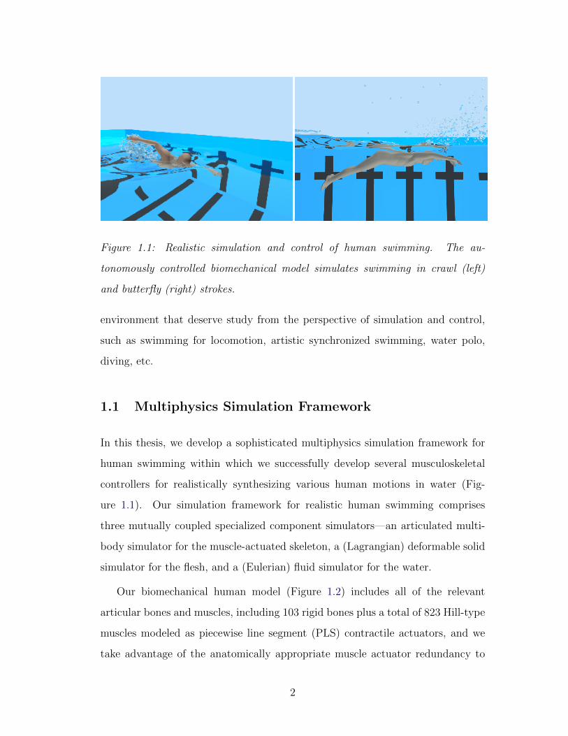
Figure 1.1: Realistic simulation and control of human swimming. The au-
tonomously controlled biomechanical model simulates swimming in crawl (left)
and butterfly (right) strokes.
environment that deserve study from the perspective of simulation and control,
such as swimming for locomotion, artistic synchronized swimming, water polo,
diving, etc.
1.1 Multiphysics Simulation Framework
In this thesis, we develop a sophisticated multiphysics simulation framework for
human swimming within which we successfully develop several musculoskeletal
controllers for realistically synthesizing various human motions in water (Fig-
ure 1.1). Our simulation framework for realistic human swimming comprises
three mutually coupled specialized component simulators—an articulated multi-
body simulator for the muscle-actuated skeleton, a (Lagrangian) deformable solid
simulator for the flesh, and a (Eulerian) fluid simulator for the water.
Our biomechanical human model (Figure 1.2) includes all of the relevant
articular bones and muscles, including 103 rigid bones plus a total of 823 Hill-type
muscles modeled as piecewise line segment (PLS) contractile actuators, and we
take advantage of the anatomically appropriate muscle actuator redundancy to
2
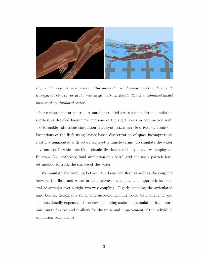
Figure 1.2: Left: A closeup view of the biomechanical human model rendered with
transparent skin to reveal the muscle geometries. Right: The biomechanical model
immersed in simulated water.
achieve robust motor control. A muscle-actuated articulated skeleton simulation
synthesizes detailed biomimetic motions of the rigid bones in conjunction with
a deformable soft tissue simulation that synthesizes muscle-driven dynamic de-
formations of the flesh using lattice-based discretization of quasi-incompressible
elasticity augmented with active contractile muscle terms. To simulate the water
environment in which the biomechanically simulated body floats, we employ an
Eulerian (Navier-Stokes) fluid simulation on a MAC grid and use a particle level
set method to track the surface of the water.
We simulate the coupling between the bone and flesh as well as the coupling
between the flesh and water in an interleaved manner. This approach has sev-
eral advantages over a tight two-way coupling. Tightly coupling the articulated
rigid bodies, deformable solid, and surrounding fluid would be challenging and
computationally expensive. Interleaved coupling makes our simulation framework
much more flexible and it allows for the reuse and improvement of the individual
simulation components.
3
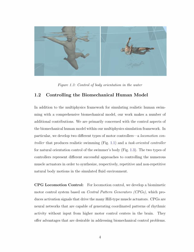
Figure 1.3: Control of body orientation in the water
1.2 Controlling the Biomechanical Human Model
In addition to the multiphysics framework for simulating realistic human swim-
ming with a comprehensive biomechanical model, our work makes a number of
additional contributions. We are primarily concerned with the control aspects of
the biomechanical human model within our multiphysics simulation framework. In
particular, we develop two different types of motor controllers—a locomotion con-
troller that produces realistic swimming (Fig. 1.1) and a task-oriented controller
for natural orientation control of the swimmer’s body (Fig. 1.3). The two types of
controllers represent different successful approaches to controlling the numerous
muscle actuators in order to synthesize, respectively, repetitive and non-repetitive
natural body motions in the simulated fluid environment.
CPG Locomotion Control: For locomotion control, we develop a biomimetic
motor control system based on Central Pattern Generators (CPGs), which pro-
duces activation signals that drive the many Hill-type muscle actuators. CPGs are
neural networks that are capable of generating coordinated patterns of rhythmic
activity without input from higher motor control centers in the brain. They
offer advantages that are desirable in addressing biomechanical control problems.
4
First, CPG models typically have just a few control parameters that modulate
the locomotion pattern. Thus, a properly implemented CPG model reduces
the dimensionality of the low-level motor control problem such that higher-level
controllers need only generate task-oriented control signals. This is one of the
most interesting features of biological CPGs. Second, CPG models typically
produce smooth modulations of the controlled trajectories, even when the control
parameters are changed abruptly. Third, CPGs produce stable rhythmic patterns,
which enable the system to rapidly return to its normal rhythmic behavior after
transient perturbations of the state variables. We create a CPG muscle controller
that produces appropriate muscle contraction forces in the virtual swimmer’s
body, which induce the human model to perform various swimming motions.
The CPG networks are divided into 10 groups to control different parts of the
body. Each CPG group comprises a number of CPG units, one unit per muscle.
Each CPG unit, which is associated with a single muscle, is modeled as a nonlinear
dynamical oscillator that can guarantee basic stability and convergence properties
of the learned control signal. Our CPG controller can generate muscle contraction
signals to produce various swimming motions by simply varying a few parameters,
and it is robust against external perturbations.
Multiobjective Task-Oriented Control: The CPG-based approach is inap-
propriate for motor control scenarios in which the required muscle contraction
signals are aperiodic. Thus, for non-locomotive, task-oriented control, we develop
a novel multiobjective control strategy that enables the biomechanical human
model to achieve the task naturally. Our method tackles the task-oriented control
problem in joint space using a multiobjective optimization approach, and then it
computes the muscle control signals needed to generate the desired joint torques.
The objective function takes into account three factors—task accomplishment,
motion naturalness, and self-collision avoidance. A new feature of this control
5
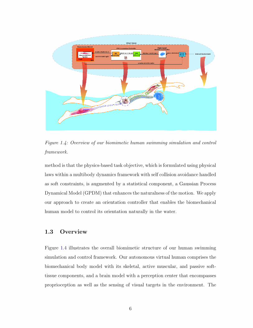
Figure 1.4: Overview of our biomimetic human swimming simulation and control
framework.
method is that the physics-based task objective, which is formulated using physical
laws within a multibody dynamics framework with self collision avoidance handled
as soft constraints, is augmented by a statistical component, a Gaussian Process
Dynamical Model (GPDM) that enhances the naturalness of the motion. We apply
our approach to create an orientation controller that enables the biomechanical
human model to control its orientation naturally in the water.
1.3 Overview
Figure 1.4 illustrates the overall biomimetic structure of our human swimming
simulation and control framework. Our autonomous virtual human comprises the
biomechanical body model with its skeletal, active muscular, and passive soft-
tissue components, and a brain model with a perception center that encompasses
proprioception as well as the sensing of visual targets in the environment. The
6
motor center of the brain has a low-level CPG locomotion controller (emulating
biological CPG networks in the spinal cord) and one that produces higher-level
motor signals such as swimming style, speed, turn direction/sharpness, etc., taking
the perceptual information into account. Given these motor signals as inputs, the
CPG networks automatically synthesize the desired muscle length signals online,
from which a proportional/derivative (PD) control mechanism produces the as-
sociated activation levels that innervate the muscles whose contractions actuate
the biomechanical body. Our multiphysics simulation framework simulates the
biomechanical human model along with the aquatic environment in which it is
situated, as well as their physical interaction.
The remainder of this thesis is organized as follows: Chapter 2 reviews relevant
prior research in the graphics, robotics, and biomechanics literature. Chapter 3
presents our multiphysics simulation framework, detailing all the simulation com-
ponents and how they are coupled in our system. The primary focal points
of this thesis are our CPG-based locomotion control and task-oriented control
through multiobjective optimization, which work within our simulation frame-
work to produce natural swimming and aquatic motions; Chapter 4 develops
our locomotion controller and Chapter 5 develops our task-oriented controller.
Chapter 6 reports our experiment results, which reveal that our complex yet
appropriately controlled human model demonstrates coordinated swimming tasks
and orientation control tasks. Chapter 7 discusses the benefits and limitations
of specific technical choices that we have made in our framework and reports on
an additional set of experiments aimed at assessing the importance of various of
its simulation/control components relative to alternative approaches. Chapter 8
presents conclusions and proposes avenues for future work.
7
CHAPTER 2
Related Work
Our work builds upon relevant technical advances in computer graphics, robotics,
and biomechanics to model the biomechanical characteristics of human body and
emulate its motor control mechanisms, as well as to simulate the continuum
mechanics of the relevant solids and fluids.
2.1 Biomechanical Human Modeling
In graphics, researchers have traditionally used joint torques to drive articulated
skeletal animation (Hodgins et al., 1995; Faloutsos et al., 2001), in contrast to
facial animation where muscle actuators have been used for two decades to syn-
thesize expressions (Waters, 1987; Lee et al., 1995). As a means of improving
realism, skeletal muscle driven motion generation is receiving growing attention
and researchers have been developing increasingly sophisticated biomechanical
models of individual body segments actuated by muscles—e.g., the arm (Albrecht
et al., 2003; Tsang et al., 2005; Sueda et al., 2008), leg (Komura et al., 2000;
Dong et al., 2002; Wang et al., 2012), neck (Lee and Terzopoulos, 2006), and
trunk (Zordan et al., 2006)—and also of the entire body (Nakamura et al., 2005).
However, the simulation of deformable flesh to produce a detailed anatomical
animation of soft tissue is missing in these previous efforts. The closest precedent
to the biomechanical human model that we have developed is the upper-body
musculoskeletal model reported in (Lee et al., 2009), which employed a one-way
coupling between flesh and bones. Ours is a full-body comprehensive human
8
model with two-way flesh-bone coupling.
2.2 Underwater Motion Simulation
Early work on simulating the underwater motions of aquatic creatures adopted
rather simple solid and fluid models: Tu and Terzopoulos (1994) simulated fishes
using a simple biomechanical model, a mass-spring-damper system to model piscine
bodies immersed in a simplified fluid model. Yang et al. (2004) used an articulated
body representation and a simplified fluid model. As the simulation techniques
for solids and fluids advance, researchers have used increasingly sophisticated fluid
models and solid-fluid coupling techniques for simulating underwater creatures.
Kwatra et al. (2010) and Tan et al. (2011) used a simplified articulated body
representation and two-way coupling between the body and a fluid simulation to
model creatures locomoting in fluids. Lentine et al. (2011) employed articulated
skeletons with a deformable skin layer and two-way coupling to a fluid simulator
to model figures moving in fluids. We too employ an articulated (human) skeleton,
but also include non-rigid simulated flesh, and use two-way coupling between the
deformable skin and water to synthesize natural human aquatic motion.
2.3 Underwater Motion Control
Motion control in underwater creatures was pioneered by Tu and Terzopoulos
(1994). Grzeszczuk and Terzopoulos (1995) achieved optimal parameters for
underwater gait behavior in rather simple creatures through spatial-temporal op-
timization methods. Tan et al. (2011) proposed a Covariance Matrix Adaptation
based optimization to create realistic swimming behavior for a given articulated
creature body. However, achieving sophisticated human swimming styles through
spatial-temporal optimization is a huge challenge as one must define a tailored
9
objective function for each style. Other methods have therefore been developed
to create gait motions for more complex systems such as humans. Yang et al.
(2004) developed a layered strategy for human swimming control in which each
control layer is procedurally modeled and empirically tuned to create physics-
based swimming motion in real time. Kwatra et al. (2010) developed a swimming
controller that computes the necessary joint torques to follow captured human
motions that mimic swimming.
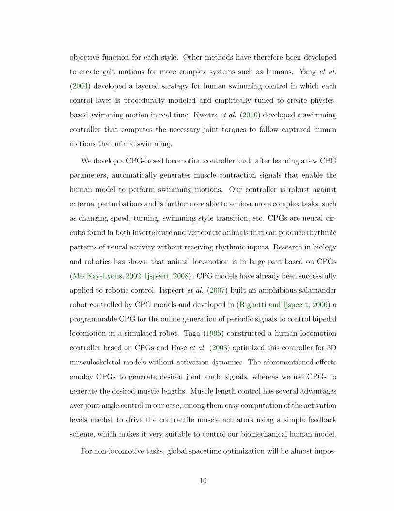
We develop a CPG-based locomotion controller that, after learning a few CPG
parameters, automatically generates muscle contraction signals that enable the
human model to perform swimming motions. Our controller is robust against
external perturbations and is furthermore able to achieve more complex tasks, such
as changing speed, turning, swimming style transition, etc. CPGs are neural cir-
cuits found in both invertebrate and vertebrate animals that can produce rhythmic
patterns of neural activity without receiving rhythmic inputs. Research in biology
and robotics has shown that animal locomotion is in large part based on CPGs
(MacKay-Lyons, 2002; Ijspeert, 2008). CPG models have already been successfully
applied to robotic control. Ijspeert et al. (2007) built an amphibious salamander
robot controlled by CPG models and developed in (Righetti and Ijspeert, 2006) a
programmable CPG for the online generation of periodic signals to control bipedal
locomotion in a simulated robot. Taga (1995) constructed a human locomotion
controller based on CPGs and Hase et al. (2003) optimized this controller for 3D
musculoskeletal models without activation dynamics. The aforementioned efforts
employ CPGs to generate desired joint angle signals, whereas we use CPGs to
generate the desired muscle lengths. Muscle length control has several advantages
over joint angle control in our case, among them easy computation of the activation
levels needed to drive the contractile muscle actuators using a simple feedback
scheme, which makes it very suitable to control our biomechanical human model.
For non-locomotive tasks, global spacetime optimization will be almost impos-
10
sible in our case; as we explain in Chapter 5, local optimization is more practical.
Lentine et al. (2011) treated motion control as an optimization problem where
rather simple creatures move by locally seeking solutions to objective functions.
Their controllers are tightly interactive to the surrounding fluid and show inter-
esting creature movement by minimizing or maximizing drag and lift. Our task-
oriented controller is also based on local optimization in time. Our multiobjective
strategy achieves natural underwater motions by augmenting the physics-based
task objective with a data-driven naturalness objective.
Physics-based simulation can generate physically plausible human motions,
but physical laws alone are insufficient to generate natural human motions, since
such motions can be physically correct yet appear unnatural. One way to address
this problem is to apply optimization strategies. Witkin and Kass (1988) postu-
lated that a physically-simulated character should minimize its effort to synthesize
a movement subject to certain constraints (see also (Grzeszczuk and Terzopoulos,
1995)). Numerous performance criteria for human motion modeling, e.g. minimal
energy, minimal torque variation, minimal jerk, etc., have been introduced by
computer animation researchers. However, to apply these performance criteria,
we generally must perform non-convex global optimization over a time interval,
which is very expensive for our case, as we discuss in Chapter 5.
Statistical approaches provide another way to get natural motion. Gaussian
Processes (GPs) and their variants (e.g., GPLVM (Lawrence, 2004), GPDM) have
recently attracted interest in computer animation for creating natural kinematic
motion, including inverse kinematics (Grochow et al., 2004), motion interpolation
(Mukai and Kuriyama, 2005), motion editing (Ikemoto et al., 2009), and motion
synthesis (Ye and Liu, 2010; Wei et al., 2011; Levine et al., 2012). While GP-
based methods are able to create natural kinematic human motions, they cannot
be directly used in physics-based controllers because, as with other data-driven
methods, the resulting motions may be physically infeasible. Wei et al. (2011)
11
proposed an approach to generate physically realistic animations that react to
perturbations by learning a nonlinear probabilistic force field function from pre-
recorded motion data using GP and combining it with physical constraints in a
probabilistic framework. Their approach is effective when the external forces are
close to those in the prerecorded motions, but it is unclear whether GP-based
methods can reliably model the external forces needed to generate motions that
are physically highly dependent on a dynamic fluid environment. Therefore, our
approach relies mainly on a physics-based control term to achieve the goal while
enhancing the naturalness of the motion using a GPDM, thereby achieving a
balance between physical realism and data-driven naturalness.
12
CHAPTER 3
Simulation and Coupling
In this chapter, we present our multiphysics simulation framework and detail how
each of its component simulators serves to animate swimming and underwater
motions using a sophisticated biomechanical human model.
3.1 Overview
Our multiphysics simulation framework for realistic human swimming comprises
three mutually coupled specialized component simulators—an articulated multi-
body simulator for the muscle-actuated skeleton, a (Lagrangian) deformable body
simulator for the flesh and muscles, and a (Eulerian) fluid simulator for the water.
Figure 3.1 illustrates the different simulation components of our multiphysics
simulation framework. Figure 3.2 illustrates the different simulation layers of
our biomechanical human model.
3.2 Biomechanical Human Simulation Components
We have developed a comprehensive biomechanical human model with 103 rigid
bones (comprising 163 articular degrees of freedom) (Figure 3.2(a)), including
the vertebrae and ribs, which is actuated by 823 muscles modeled as piecewise
uniaxial Hill-type contractile actuators (Figure 3.2(b)). The skeleton is simulated
as an articulated, multibody dynamical system. The 3D muscle and passive
flesh simulation is accomplished by deforming a lattice-based discretization of
13
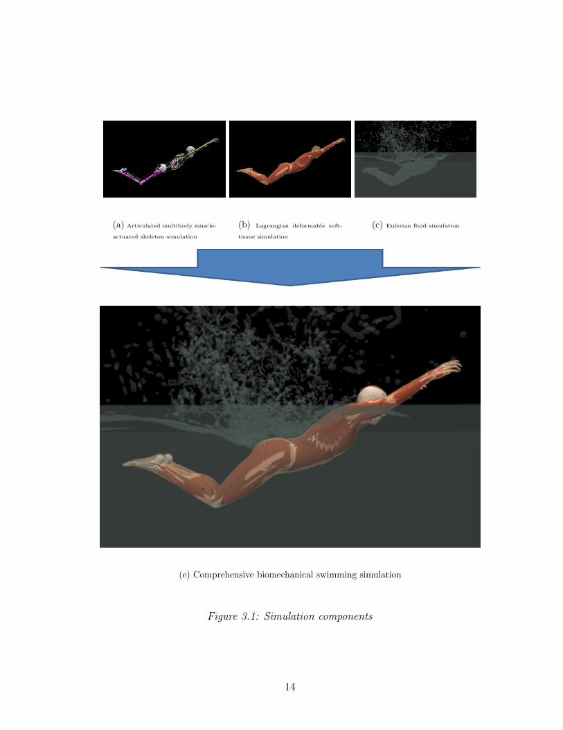
(a) Articulated multibody muscle-
actuated skeleton simulation
(b) Lagrangian deformable soft-
tissue simulation
(c) Eulerian fluid simulation
(e) Comprehensive biomechanical swimming simulation
Figure 3.1: Simulation components
14
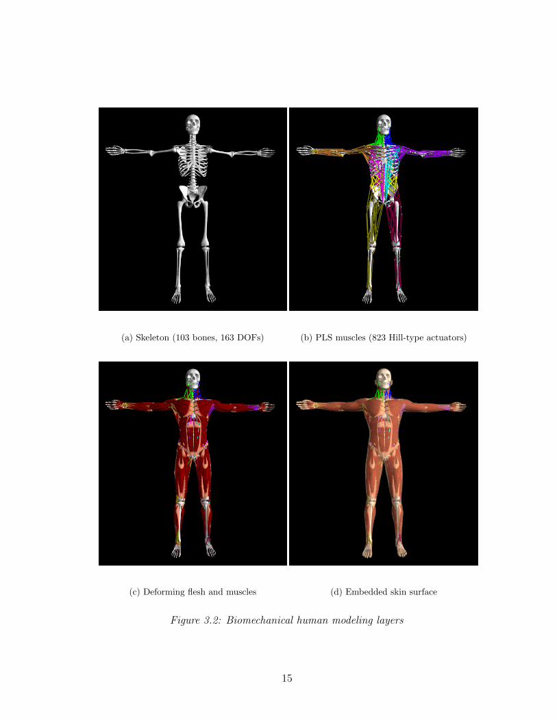
(a) Skeleton (103 bones, 163 DOFs) (b) PLS muscles (823 Hill-type actuators)
(c) Deforming flesh and muscles (d) Embedded skin surface
Figure 3.2: Biomechanical human modeling layers
15
quasi-incompressible elastic material augmented with active muscle terms (Fig-
ure 3.2(c)). The inertial properties of the skeleton are approximated from the
dense volumetric physical parameters of the soft-tissue elements—each bone’s
inertial tensor is augmented by the inertial parameters of its associated soft
tissues. The natural dynamics of the simulated human are induced by muscle
forces generated by the contractile actuators.
The low-level motor control inputs of our biomechanical human model com-
prise the activation levels of each muscle actuator in the simulated body. The
activated muscles generate forces that drive the skeletal simulation. Given the
contractile muscle forces, plus the external forces from the flesh simulation, we
simulate the skeleton using the Articulated Body Method (Featherstone, 1987)
to compute the forward dynamics in conjunction with a backward Euler time-
integration scheme as in (Lee et al., 2009). For the purpose of simulating the
dynamic deformation of the flesh and muscles, we employ a lattice-based dis-
cretization of quasi-incompressible elasticity augmented with active muscle terms.
This approach avoids the need for multiple meshes conforming to individual
muscles and its regular structure offers significant opportunities for performance
optimizations.
3.2.1 Muscle-Actuated Skeleton Simulation
The force generating characteristic of the piecewise uniaxial contractile muscle is
governed by a linearized Hill-type model (Lee et al., 2009). Assuming that the
length of the tendon is constant, we model a muscle force as the sum of forces
from a contractile element (CE), which represents the active muscle force that is
controlled by the motor neurons, and a parallel element (PE), which accounts for
the passive elasticity of the muscle (Fung, 1993).
The passive elasticity PE force is modeled as a unidirectional exponential
16
spring:
fP = max (0, ks (exp(kce)− 1) + kde) , (3.1)
where ks, kc, and kd are elastic and damping coefficients, e = (l − l0)/l0 is the
strain of the muscle, with l and l0 its length and slack length, respectively, and
e = l/l0 is the strain rate.
The CE represents the active muscle force controlled by the motor neurons as
fC = aFl(l)Fv(l), (3.2)
where 0 ≤ a ≤ 1 is the activation level of the muscle. Force fC depends on
the length and velocity of a muscle. The force-length relation is modeled as
Fl(l) = max(0, kmax(l − lm)), where kmax is the maximum stiffness of a fully
activated muscle and lm is the minimum length at which the muscle can produce
force. The force-velocity relation is modeled as Fv(l) = max(0, 1 + min(l, 0)/vm),
where vm(≥ 0) is the maximum contraction velocity under no load. The control
input to the skeleton simulation is the activation level a of each muscle. Chapters 4
and 5 present how our motor controllers determine these muscle activation levels.
Given the muscle forces and other external forces (e.g., gravity.), we perform
the simulation of the skeleton using the Articulated Body Method (Featherstone,
1987) for solving the forward dynamics and the backward Euler time-integration
scheme.
3.2.2 Soft-Tissue Simulation
The elastic flesh and musculature serves as an intermediary between the fluid
environment and the articulated skeleton. The shape and deformation of the
flesh volume is determined by the dynamics of the articulated skeleton and the
hydrodynamic forces acting on the flesh. Naturally, the exact tissue behavior is
also dependent on the geometric layout and material properties of the heteroge-
neous array of tissue components that constitute the flesh. Some of these material
17
traits are encoded as static distributions of scalar (e.g., elastic moduli) or vector
(e.g., muscle fiber orientation) quantities; other material properties, such as the
muscle activations, are time-varying signals that are provided as input to the flesh
simulation along with the skeletal dynamics.
We capture the physical behavior of the human swimmer’s soft tissue and
musculature via numerical simulation of a discrete volumetric model. In designing
this discrete representation, we commit to certain simplifying assumptions and
modeling approximations to strike a reasonable balance between computational
complexity, geometric resolution, biomechanical accuracy and robustness of sim-
ulation. First, we do not separately model the skin as a distinct simulation
component; for the purposes of fluid-flesh interaction, the contact surface is sim-
ply the boundary of the flesh volume and not a separate two-dimensional skin
layer. The entirety of the space between the skin and bones is modeled as an
elastic continuum; no air-filled cavities or fluid volumes are explicitly simulated
as such, although we are free to modulate the elastic properties (e.g., stiffness or
compressibility) of such areas to reflect their macroscopic behavior. In addition,
the entire flesh volume is assumed to deform as a connected continuum; that is,
we do not allow slip or separation in the interior of the flesh volume. Note that
connective tissue typically limits the extent of such motions, but there are parts
of anatomy where true sliding or separation is possible in the real human body.
For the purpose of simulating the dynamic deformation of flesh and muscle,
we employ a lattice-based discretization of quasi-incompressible elasticity aug-
mented with active (contractile) muscle terms. The lattice-based representation
(in essence, a lattice deformer) captures the shape of the deforming flesh volume.
This discrete model is simply created by superimposing a cubic lattice (we use a
lattice size of 10 mm) on a three-dimensional model of the human body, and we
discard all cells that do not intersect the flesh volume (i.e., cells that are outside
the body, or wholly within solid bones). Of course, the lattice representation thus
18
created does not accurately capture the geometry of the flesh volume, but provides
only a “cubed” approximation. Despite this, we construct the discrete governing
equations so as to compensate for this geometric discrepancy. We discretize the
equations of elasticity following the methodology of (Patterson et al., 2012), which
captures the fact that lattice elements on the boundary of the flesh volume are
only fractionally covered by elastic material. The jagged boundary of the lattice-
derived simulation volume also differs from the actual skin surface where fluid
forces are to be applied; we compensate for that by embedding a high-resolution
skin surface mesh within the cubic lattice (Figure 3.2(d)) and distributing the
forces acting on the skin surface into the volumetric lattice by scaling with the
appropriate embedding weights as discussed in (Zhu et al., 2010). Finally, since the
contact surface between the flesh and bones is not resolved in the lattice-derived
mesh, we use stiff zero-rest-length springs to elastically attach points sampled on
bone surfaces to embedded locations in the flesh simulation lattice, as detailed by
(Lee et al., 2009; McAdams et al., 2011).
3.2.2.1 Flesh Constitutive Model
The deformable collection of flesh, skin, and muscle are modeled as a hyperelastic
solid. The elastic energy associated with it is partitioned as follows:
Etotal = Eiso + Emuscle + Evol + Eatt. (3.3)
In this expression, Eiso =∫
ΩΨiso(F)dX is a strain energy of an isotropic “foun-
dation” material which corresponds to passive flesh (predominantly fatty tissue),
where F = ∂φ/∂X denotes the deformation gradient of the 3D deformation
function φ : Ω→ R3, which maps material coordinates X to world-space deformed
locations x = φ(X). For the subset Ωm of the body, which is covered by muscle,
an additional anisotropic energy term Emuscle =∫
ΩmΨmuscle(F)dX is added, to
account for the directional passive/active response of fibrous muscle tissue. The
19
energy term Evol enforces volume preservation in the flesh. Finally, the energy
term Eatt is associated with the elastic attachment constraints that couple the
flesh and bone.
The isotropic component of the strain energy density is formulated as a Mooney-
Rivlin material
Ψiso(F) = µ10(‖F‖2F − 3) +
µ01
2(‖F‖4
F − ‖FTF‖2F − 6) (3.4)
with parameter values µ10 = 20 KPa, µ01 = 60 KPa. Note that we use a simple,
non-deviatoric formulation of Mooney-Rivlin hyperelasticity. Our formulation
supports strong incompressibility; thus, factoring out the hydrostatic stress com-
ponent is not essential (F will be forced to have unit determinant by means of
the strong incompressibility penalty). The anisotropic component of the strain
energy is expressed as:
Ψmuscle =∑k
Ψ(k)m (F; wk; ak) [X covered by muscle k], (3.5)
where wk and ak are the fiber direction and activation level of the k-th muscle,
respectively. The energy density term associated with the k-th muscle is a function
Ψ(k)m (λk, ak) of the along-fiber stretch ratio λk = ‖Fwk‖2 and the respective
activation value ak. Quantity Ψ(k)m is defined indirectly through its derivative with
respect to λk; in fact, ∂Ψ(k)m /∂λk = T (λk, ak) is the directional tension function
resulting from the sum of the passive elasticity and force-length terms used in
the muscle-actuated skeleton simulation. The strain rate and force-velocity terms
have been omitted for simplicity, a decision further motivated by the fact that we
use a non-validated generic Rayleigh damping model for the isotropic flesh, which
would dilute the accuracy of an elaborate force-velocity formulation.
3.2.2.2 Incompressibility
We enforce volume preservation in the elastic material via a penalty term Evol =∫Ω
Ψvol(J)dX, where Ψvol(J) = κ log2(J)/2, with J = det F, is the volume
20
change ratio, and the bulk modulus κ is set to 20 MPa. In order to improve
the numerical conditioning of this quasi-incompressible material, we transition to
a mixed displacement/pressure energy formulation:
E(x, p) = Eatt +
∫Ω
[Ψiso(F) + Ψmuscle(F) + αp log(J)− α2p2
2κ
]dX. (3.6)
As is known from the theory of mixed discretizations, the spatial gradients f =
−∂E/∂x and f = −∂E/∂x of the two energy formulas (corresponding to elastic
forces) are equal when the mixed energy E is stationary with respect to a variation
in the pressure field. Thus, we construct a time-integration scheme by computing
forces according to f(x, p) = −∂E(x, p)/∂x, and append the stationarity condi-
tion ∂E/∂p = 0 to the time integration equations. The result obtained is the
same as the pure-displacement formulation, but the discrete equations remain
well conditioned regardless of the degree of incompressibility. The price we pay
for this favorable conditioning is that the discrete time integration equations
become symmetric indefinite, thus a Krylov solver such as MINRES, SYMMLQ,
or symmetric QMR must be used in place of Conjugate Gradients.
3.2.2.3 Skeletal Attachments
Since the surfaces of attachment between flesh and bone do not coincide with
nodes of the simulation lattice, we enforce such attachments via soft, spring-based
constraints. The attachment energy Eatt is formulated as:
Eatt(x) =∑i
ki2‖Wix− ti‖2
2, (3.7)
where ti is the target location (on the moving skeleton) of a flesh attachment, Wi
is a trilinear interpolation operator that computes the interpolated location of an
interior flesh point from the vector of nodal positions x, and ki is the stiffness
parameter of the i-th attachment. Attachment points are discretely sampled as a
preprocess on the bone surfaces. Attachment points are sampled uniformly, with
21
a target density that yields an average of 3 to 6 attachment points per cell of
the simulation lattice. The stiffness parameters are adapted such that a constant
stiffness per bone surface area is achieved.
3.2.2.4 Discretization Given Musculature and Skeletal Structure
We use standard trilinear hexahedral elements on a cubic lattice for the discretiza-
tion of the deformation map φ, while the pressure field is only approximated as
cell-wise constant. The geometries of the skin, muscles and bones are embedded
in the simulated hexahedra. We use the geometry of the muscles to modulate
the material properties assigned to each simulation element. We compute the
nonlinear energy integrals by defining a 4-point quadrature rule on an individual
lattice cell basis, which is designed to be accurate in the integration of polynomials
of degree up to 2, yielding a (locally) second-order accurate approximation to the
energy.
To achieve second-order accuracy on arbitrarily integration domains, we use a
numerical quadrature scheme that integrates exactly all monomials XpY qZr with
0 ≤ p + q + r ≤ 2; i.e., we provide the following quadrature (Patterson et al.,
2012):
∫Ωk
1 X Y Z
X X2 XY XZ
Y XY Y 2 Y Z
Z XZ Y Z Z2
dX. (3.8)
Here X = (X, Y, Z) is the material point in the undeformed configuration and
Ωk = Ω ∩ Ck is the elastic sub-domain within each lattice cell Ck.
In our implementation, we use Monte-Carlo integration to compute the rel-
evant moments of fractional cells Ck. A number of randomly generated points
are uniformly distributed in each simulation hexahedron, indicated as colored
22
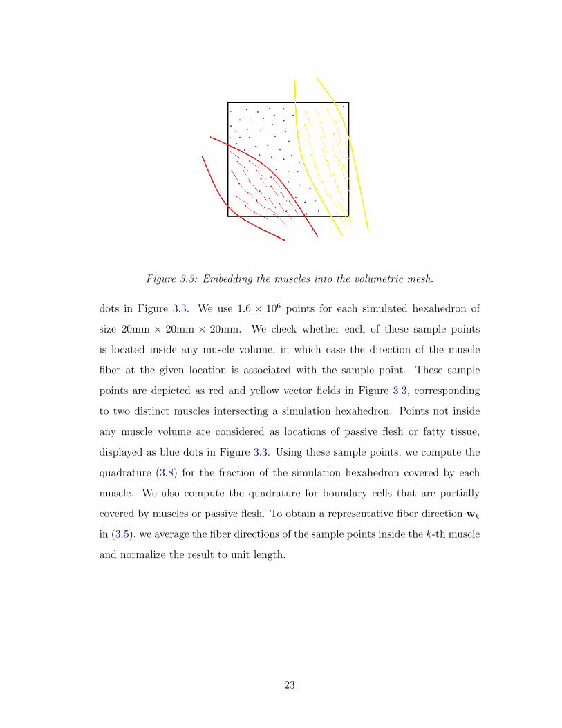
Figure 3.3: Embedding the muscles into the volumetric mesh.
dots in Figure 3.3. We use 1.6 × 10⁶ points for each simulated hexahedron of
size 20mm × 20mm × 20mm. We check whether each of these sample points
is located inside any muscle volume, in which case the direction of the muscle
fiber at the given location is associated with the sample point. These sample
points are depicted as red and yellow vector fields in Figure 3.3, corresponding
to two distinct muscles intersecting a simulation hexahedron. Points not inside
any muscle volume are considered as locations of passive flesh or fatty tissue,
displayed as blue dots in Figure 3.3. Using these sample points, we compute the
quadrature (3.8) for the fraction of the simulation hexahedron covered by each
muscle. We also compute the quadrature for boundary cells that are partially
covered by muscles or passive flesh. To obtain a representative fiber direction wk
in (3.5), we average the fiber directions of the sample points inside the k-th muscle
and normalize the result to unit length.
23
3.3 Water Simulation
The surrounding water in which our biomechanical human model floats is simu-
lated according to the Navier-Stokes equations using an Eulerian fluid solver on
a MAC grid, and the water surface is tracked using the particle level-set method,
which is in accordance with (Enright et al., 2002) and (Foster and Fedkiw, 2001).
Our simulation framework implements the necessary dynamic force couplings
between the skeleton and flesh, as well as between the deformable skin surface
of the virtual human and the surrounding water, in an interleaved manner.
The fluid simulation system we use is part of PhysBAM,1 which is an object
oriented C++ library capable of solving a variety of problems in computational
fluid dynamics, computational mechanics, computer graphics and computer vi-
sion. The approach to model the water surface is called the “particle level set
method” (Enright et al., 2002), which is a hybrid surface tracking method that uses
massless marker particles combined with a dynamic implicit surface. This hybrid
surface model has advantages of both particle evolution and level set evolution. To
elaborate, level set evolution suffers from volume loss near detailed features while
particle evolution suffers from visual artifacts in the surface when the number of
particles is small. Conversely, the level set is always smooth, and particles retain
detail regardless of flow complexity. They tend to have complementary strength
and weakness, a combined approach gives superior results under a wider variety
of situations.
3.3.1 Outline of the Fluid Simulation Method
The Navier-Stokes equations for describing the motion of a liquid consist of two
parts. The first enforces incompressibility by dictating that mass should always
1See http://physbam.stanford.edu
24
be conserved; i.e.,
∇ · u = 0, (3.9)
where u is the liquid velocity field, and
∇ = (∂/∂x, ∂/∂y, ∂/∂z) (3.10)
is the gradient operator. The second equation couples the velocity and pressure
fields and relates them through the conservation of momentum; i.e.,
ut = ν∇ · (∇u)− (u · ∇) u− 1
ρ∇p+ g. (3.11)
This equation models the changes in the velocity field over time due to the effects
of viscosity ν, convection, density ρ, pressure p, and gravity g. By solving and
over time, we can simulate the behavior of a volume of liquid. The basic algorithm
(Foster and Fedkiw, 2001) is as follows:
1. Model the static environment as a voxel grid.
2. Model the liquid volume using a combination of particles and an implicit
surface.
3. Update the velocity field by solving (3.11) using finite differences combined
with a semi-Lagrangian method.
4. Apply velocity constraints due to moving objects.
5. Enforce incompressibility by solving a linear system built from (3.9).
6. Update the position of the liquid volume (particles and implicit surface)
using the new velocity field.
Enright et al. (2002) improved this algorithm by introducing a new “thickend”
front-tracking technique to accurately represent the water surface and a new
25
velocity extrapolation method to move the surface in a smooth, water-like manner.
The focus is to maintain the liquid surface itself. Particles are placed on both sides
of the surface and used to maintain an accurate representation of the surface itself
regardless of what may be on one side or the other. The particles are intended to
correct errors in the surface representation by the implicit function.
3.4 Flesh-Water Coupling
The traditional method for coupling fluids and solids is for the solid to prescribe
velocity boundary conditions on the fluid and for the fluid to provide force bound-
ary conditions on the solid (Benson, 1992). Accordingly, we also use the velocity of
the human body model skin surface to enforce the Neumann boundary condition
along the surface by making the normal component of the fluid velocity equal to
the normal component of the skin’s velocity. To calculate the force of the fluid
on the body, we would ideally integrate over the surface of the skin the pressure
computed by the fluid solver.
For incompressible flow, however, the pressure (which serves as a penalty
term in the Navier-Stokes computation) is both stiff and noisy, hence more or
less unreliable, as discussed in (Fedkiw, 2002). While the velocity field is a
primary state variable and is limited in its temporal variation due to momentum
conservation, the pressure field is a byproduct of the projection of velocities into
a divergence-free field, and may exhibit notably higher temporal variance than
the fluid velocities. As a consequence, instead of demanding a higher degree of
accuracy in the pressure computation from our underlying fluid simulation engine,
we opt for a computation of fluid-to-solid forces based on fluid velocities, which are
generally more accurate and temporally coherent. We use the relative velocity of
the human skin with respect to the fluid to compute the hydrodynamic force and
we construct a new level-set representation of the water to compute the buoyancy
26
force. These forces due to the water acting on the body are computed at each
triangle of the skin surface and applied to the skin as external forces.
To compute the hydrodynamic force on each triangle of the skin surface, we
employ a hydrodynamic force model similar to those found in (Tu and Terzopoulos,
1994; Yang et al., 2004; Lentine et al., 2011):
f = min [0,−ρA (n · v)] (n · v) n, (3.12)
where ρ is the density of the water, A is the area of the triangle, n is its normal,
and v is its velocity relative to the water. To enforce the boundary conditions in
the fluid solver, we must make the normal component of the fluid velocity equal to
the normal component of the solid’s velocity, so we cannot use the fluid velocity on
the boundary cell to compute the relative velocity as its normal component will be
approximately zero. Instead, we accumulate velocities of the fluid in neighboring
cells around the boundary cell in which the skin triangle lies and employ the mean
local fluid velocity to compute the relative velocity v.
The total buoyancy force acting on the floating body equals the weight of
water displaced by the body. For underwater motion with the body wholly
immersed, the buoyancy approximately cancels out the gravity force, since the
average density of the human body approximately equals the density of water.
However, this is not the case for swimming where the human body is often only
partially immersed. It is then very important to compute buoyancy correctly
in order to simulate realistic dynamic trunk motions, especially for the butterfly
swimming stroke. We can represent the buoyancy as B = −ρgV , where g is the
gravitational acceleration, and V is the volume of water displaced by the body.
We may rewrite this as
B = ρg
∫S
h(n · j)dA, (3.13)
where S is the immersed surface of the body model, n is the normal of the area
element, j is the upward unit vector, and h denotes the distance from the water
27
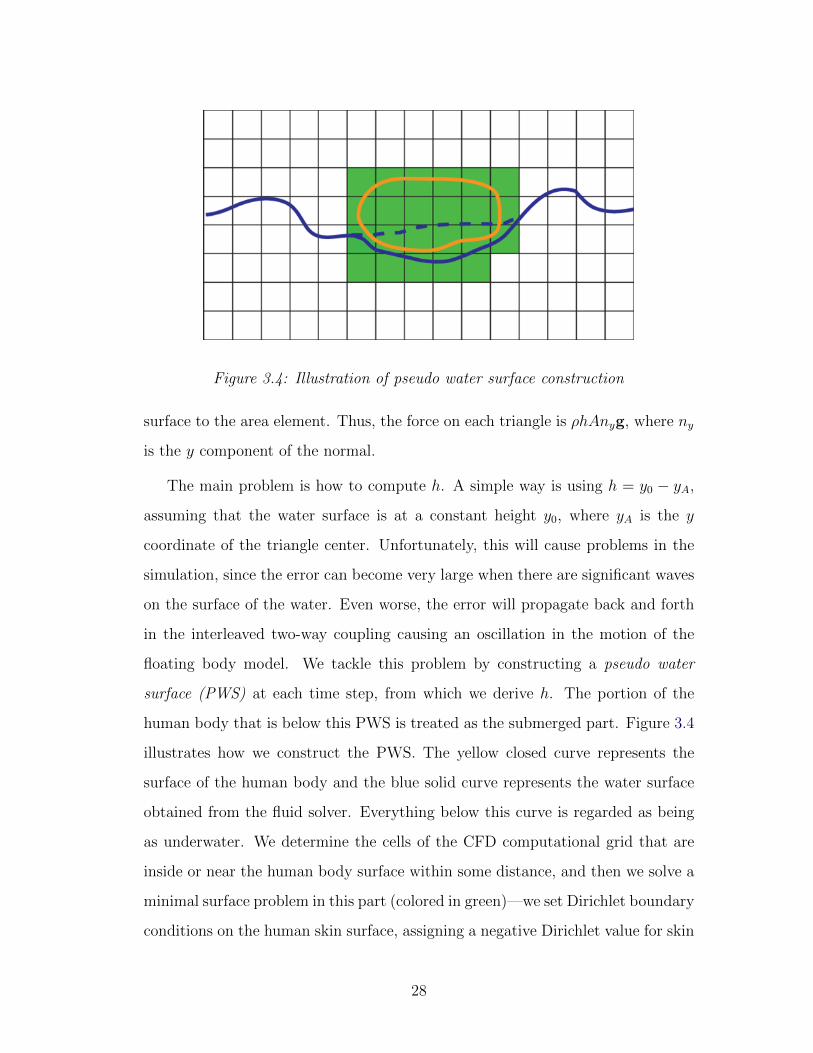
Figure 3.4: Illustration of pseudo water surface construction
surface to the area element. Thus, the force on each triangle is ρhAnyg, where ny
is the y component of the normal.
The main problem is how to compute h. A simple way is using h = y0 − yA,
assuming that the water surface is at a constant height y0, where yA is the y
coordinate of the triangle center. Unfortunately, this will cause problems in the
simulation, since the error can become very large when there are significant waves
on the surface of the water. Even worse, the error will propagate back and forth
in the interleaved two-way coupling causing an oscillation in the motion of the
floating body model. We tackle this problem by constructing a pseudo water
surface (PWS) at each time step, from which we derive h. The portion of the
human body that is below this PWS is treated as the submerged part. Figure 3.4
illustrates how we construct the PWS. The yellow closed curve represents the
surface of the human body and the blue solid curve represents the water surface
obtained from the fluid solver. Everything below this curve is regarded as being
as underwater. We determine the cells of the CFD computational grid that are
inside or near the human body surface within some distance, and then we solve a
minimal surface problem in this part (colored in green)—we set Dirichlet boundary
conditions on the human skin surface, assigning a negative Dirichlet value for skin
28
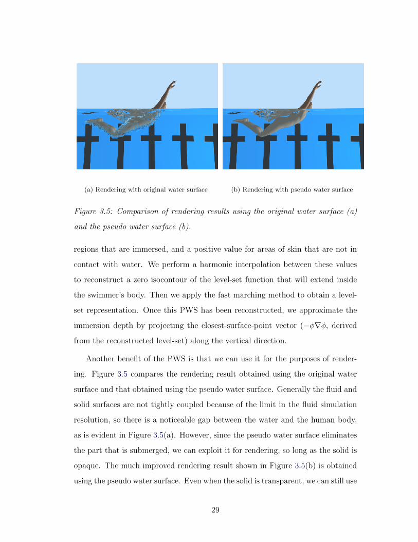
(a) Rendering with original water surface (b) Rendering with pseudo water surface
Figure 3.5: Comparison of rendering results using the original water surface (a)
and the pseudo water surface (b).
regions that are immersed, and a positive value for areas of skin that are not in
contact with water. We perform a harmonic interpolation between these values
to reconstruct a zero isocontour of the level-set function that will extend inside
the swimmer’s body. Then we apply the fast marching method to obtain a level-
set representation. Once this PWS has been reconstructed, we approximate the
immersion depth by projecting the closest-surface-point vector (−φ∇φ, derived
from the reconstructed level-set) along the vertical direction.
Another benefit of the PWS is that we can use it for the purposes of render-
ing. Figure 3.5 compares the rendering result obtained using the original water
surface and that obtained using the pseudo water surface. Generally the fluid and
solid surfaces are not tightly coupled because of the limit in the fluid simulation
resolution, so there is a noticeable gap between the water and the human body,
as is evident in Figure 3.5(a). However, since the pseudo water surface eliminates
the part that is submerged, we can exploit it for rendering, so long as the solid is
opaque. The much improved rendering result shown in Figure 3.5(b) is obtained
using the pseudo water surface. Even when the solid is transparent, we can still use
29
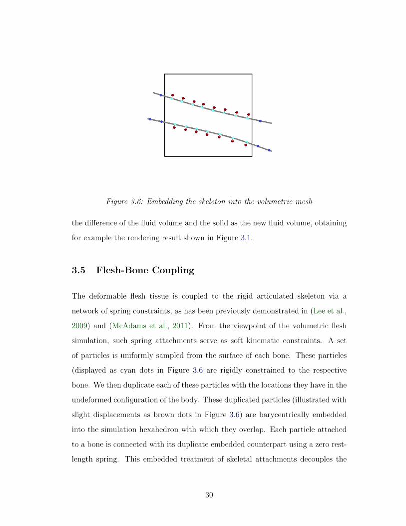
Figure 3.6: Embedding the skeleton into the volumetric mesh
the difference of the fluid volume and the solid as the new fluid volume, obtaining
for example the rendering result shown in Figure 3.1.
3.5 Flesh-Bone Coupling
The deformable flesh tissue is coupled to the rigid articulated skeleton via a
network of spring constraints, as has been previously demonstrated in (Lee et al.,
2009) and (McAdams et al., 2011). From the viewpoint of the volumetric flesh
simulation, such spring attachments serve as soft kinematic constraints. A set
of particles is uniformly sampled from the surface of each bone. These particles
(displayed as cyan dots in Figure 3.6 are rigidly constrained to the respective
bone. We then duplicate each of these particles with the locations they have in the
undeformed configuration of the body. These duplicated particles (illustrated with
slight displacements as brown dots in Figure 3.6) are barycentrically embedded
into the simulation hexahedron with which they overlap. Each particle attached
to a bone is connected with its duplicate embedded counterpart using a zero rest-
length spring. This embedded treatment of skeletal attachments decouples the
30
resolution of the simulation mesh from the resolution of the skeletal geometry and
allows us to define the attachment regions as arbitrary point-sampled surfaces.
In our framework, we further leverage this network of soft constraints to
transfer to the bones external forces that are applied to the skin surface, in a
manner that respects the deformable flesh medium that separates the point of
application of such forces (the skin forces) from the location of the bones. After
computing the distribution of external forces on the skin, originating from any
sources including fluid forces or collisions, we solve for the quasi-static equilibrium
shape of the deformable flesh. Once the steady state configuration has been
computed, the tension of the attachment springs is used to calculate how the skin-
applied forces have been distributed to the bone-flesh interface. From balance of
force properties, we have strong guarantees that the aggregate force applied by
the attachment springs to the bones (at equilibrium), independent of the material
parameters of the soft tissue or the stiffness of the attachment springs; of course,
different material parameters may have an effect on how broadly a surface force
gets spread out from the point of application. This quasi-static process makes the
force translation from the flesh to the bones occur instantaneously. Although this
eliminates a potential lag, the external forces on the skin or flesh are well spread
to the bones in a natural way.
Appendix B discusses an for improving the flesh-bone coupling by employing
the Jacobian matrix of the external translated force with respect to the generalized
coordinates of the skeleton.
3.6 Summary
We have introduced a multiphysics simulation and control framework whose over-
all architecture is shown in Figure 1.4. The inputs to our biomechanical human
model are the muscle activation levels, which drive both the Hill-type PLS muscles
31
that actuate the skeleton and the flesh simulation. The skeleton, flesh, and
water are two-way coupled in an interleaved manner. To synthesize realistic
human motion within this framework, we still need to design motor controllers
that generate proper muscle activation levels to produce swimming and other
aquatic motions. Our biomechanical human model also provides proprioceptive
feedback, such as muscle lengths, joint angles, joint velocities, body orientation,
etc., to the motor controllers. Within our simulation framework, we will proceed
to develop two different types of motor controllers—locomotion controllers that
produce realistic swimming and task-oriented controllers for natural underwater
orientation control of the swimmer’s body. Chapters 4 and Chapter 5 will present
the details of these two types of controllers, respectively.
32
CHAPTER 4
CPG Locomotion Control
The control of biomechanically simulated human swimming is a challenging prob-
lem. Swimming motions have several distinctive styles, such as the butterfly and
the crawl, each of which requires the coordinated rhythmic movement of multiple
body segments.
Biological CPGs are neural networks capable of generating stable patterns
of rhythmic activity without any input from higher motor control centers in
the brain. In addressing biomechanical locomotion control problems such as
swimming, CPG models offer important advantages, including the ability to eas-
ily modulate the rhythmic patterns. We employ CPGs to specify the desired
temporally-varying length of each muscle in the swimmer’s body and then apply
a feedback control loop to generate the necessary muscle activation levels. This
results in an easy-to-use locomotion controller that can enable various tasks, such
as changing speed, turning, and transitioning between swimming strokes.
The following section details the implementation of CPG control in our biome-
chanical human model for the purpose of swimming simulation. Figure 4.1 shows
the overall structure of our CPG locomotion control framework. The temporally-
varying muscle length signals as well as their first-order and second-order deriva-
tives serve as training data, and the necessary parameters for our CPG system
are learned using Incremental Locally Weighted Regression (ILWR) (Schaal and
Atkeson, 1997). The learning process, which is framed in the figure by the dashed
rectangle, need only be done once, offline, and in advance. After learning, our
33
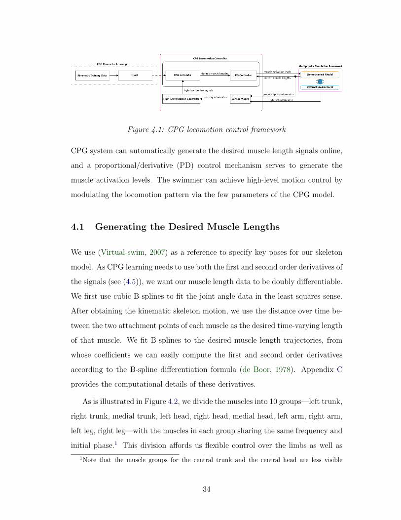
Figure 4.1: CPG locomotion control framework
CPG system can automatically generate the desired muscle length signals online,
and a proportional/derivative (PD) control mechanism serves to generate the
muscle activation levels. The swimmer can achieve high-level motion control by
modulating the locomotion pattern via the few parameters of the CPG model.
4.1 Generating the Desired Muscle Lengths
We use (Virtual-swim, 2007) as a reference to specify key poses for our skeleton
model. As CPG learning needs to use both the first and second order derivatives of
the signals (see (4.5)), we want our muscle length data to be doubly differentiable.
We first use cubic B-splines to fit the joint angle data in the least squares sense.
After obtaining the kinematic skeleton motion, we use the distance over time be-
tween the two attachment points of each muscle as the desired time-varying length
of that muscle. We fit B-splines to the desired muscle length trajectories, from
whose coefficients we can easily compute the first and second order derivatives
according to the B-spline differentiation formula (de Boor, 1978). Appendix C
provides the computational details of these derivatives.
As is illustrated in Figure 4.2, we divide the muscles into 10 groups—left trunk,
right trunk, medial trunk, left head, right head, medial head, left arm, right arm,
left leg, right leg—with the muscles in each group sharing the same frequency and
initial phase.1 This division affords us flexible control over the limbs as well as
1Note that the muscle groups for the central trunk and the central head are less visible
34
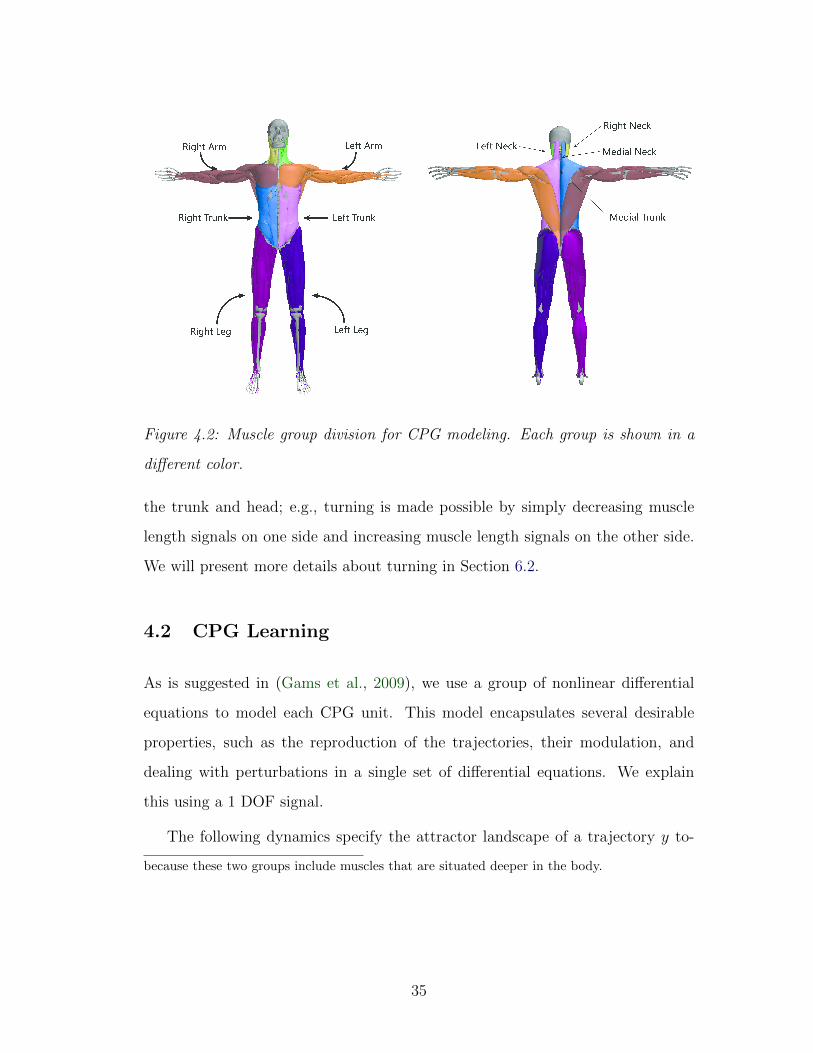
Figure 4.2: Muscle group division for CPG modeling. Each group is shown in a
different color.
the trunk and head; e.g., turning is made possible by simply decreasing muscle
length signals on one side and increasing muscle length signals on the other side.
We will present more details about turning in Section 6.2.
4.2 CPG Learning
As is suggested in (Gams et al., 2009), we use a group of nonlinear differential
equations to model each CPG unit. This model encapsulates several desirable
properties, such as the reproduction of the trajectories, their modulation, and
dealing with perturbations in a single set of differential equations. We explain
this using a 1 DOF signal.
The following dynamics specify the attractor landscape of a trajectory y to-
because these two groups include muscles that are situated deeper in the body.
35
wards the anchor point g:
z = Ω
(αz (βz (g − y)− z) +
ΣNi=1Ψiwir
ΣNi=1Ψi
)(4.1)
y = Ωz (4.2)
Ψi = exp (h (cos (Φ− ci)− 1)) (4.3)
Here, y(t) is the generated signal, z(t) is an intermediate variable that describes
the first order derivative of y, and Φ is the phase of the signal. Ω is the fundamental
frequency (lowest non-zero frequency) of the input signals. Since swimming is a
periodic motion, we can specify Ω as 2πT
, where T is the period of one swimming
cycle. The positive constants αz and βz are set to αz = 8 and βz = 2 for all
our simulations. The signal trajectory oscillates round g, an anchor point for the
oscillatory trajectory. The number of Gaussian-like periodic kernel functions Ψi
is N and h determines the width of the kernel function. We set N = 25 and
h = 2.5N for all our simulations, and ci are equally spaced between 0 and 2π in
N steps. The amplitude control parameter is r, which we set to 1.0.
In a single set of differential equations, the above model encapsulates several
desirable properties, such as approximating the desired trajectories, offering the
ability to modulate them, and maintaining robustness against perturbations.
We use ILWR to learn the weights wi in (4.1). Locally weighted regression
corresponds to finding, for each kernel function Ψi, the weight vector wi that
minimizes the quadratic error criterion
Ji =P∑t=1
Ψi(t)(ftarg(t)− wir(t)
)2, (4.4)
where the index t denotes the discrete time step,
ftarg =1
Ω2ytrain − αz
(βz (g − ytrain)− 1
Ωytrain
)(4.5)
36
The formulation of the above equations can be found in (Gams et al., 2009). As the
input into the learning algorithm, ytrain, ytrain and ytrain are the muscle length
signal, and its first and second derivatives, respectively. Incremental regression
to determine the parameters wi is accomplished with the use of recursive least
squares with a forgetting factor of λ. Given the target data ftarg(t) and r(t),
weight wi is updated by
wi(t+ 1) = wi(t) + ΨiPi(t+ 1)r(t)er(t), (4.6)
where P is the inverse covariance matrix (Ljung and Soderstrom, 1983), which is
updated as
Pi(t+ 1) =1
λ
(Pi(t)−
Pi(t)2r(t)2
λΨi
+ Pi(t)r(t)2
), (4.7)
and
er(t) = ftarg(t)− wi(t)r(t). (4.8)
The recursion is started with wi = 0 and Pi = 1. Batch and incremental
learning regressions provide identical weights wi for the same training sets when
the forgetting factor λ is set to 1.0. Differences appear when the forgetting factor
is less than 1.0, in which case the incremental regression gives more weight to
recent data. In our experiments, we set λ = 0.95.
A desirable property of the CPG control model is that it allows easy mod-
ulation of the signals. Changing the parameter g modulates the baseline of the
rhythmic movement. This will smoothly shift the oscillation without modifying
the signal shape. Modifying Ω and r changes of the frequency and the amplitude
of the oscillations, respectively. Since our differential equations are of second
order, even an abrupt change of the parameters yield smooth variations of the
trajectory y. Although the length trajectories of different muscles may share the
same frequency, the amplitudes and baseline may vary significantly. To guarantee
37
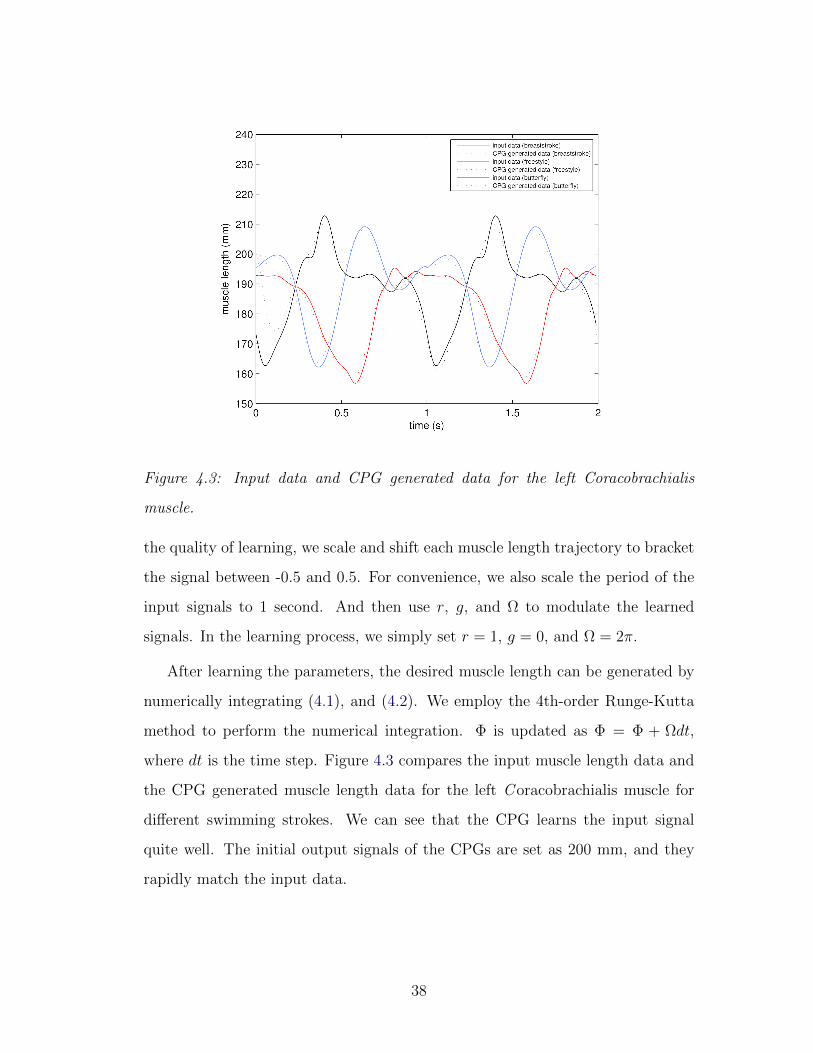
Figure 4.3: Input data and CPG generated data for the left Coracobrachialis
muscle.
the quality of learning, we scale and shift each muscle length trajectory to bracket
the signal between -0.5 and 0.5. For convenience, we also scale the period of the
input signals to 1 second. And then use r, g, and Ω to modulate the learned
signals. In the learning process, we simply set r = 1, g = 0, and Ω = 2π.
After learning the parameters, the desired muscle length can be generated by
numerically integrating (4.1), and (4.2). We employ the 4th-order Runge-Kutta
method to perform the numerical integration. Φ is updated as Φ = Φ + Ωdt,
where dt is the time step. Figure 4.3 compares the input muscle length data and
the CPG generated muscle length data for the left C oracobrachialis muscle for
different swimming strokes. We can see that the CPG learns the input signal
quite well. The initial output signals of the CPGs are set as 200 mm, and they
rapidly match the input data.
38
4.3 Muscle Control
Given the CPG-generated, time-varying length for each muscle, we use a first-
order PD control mechanism to compute the muscle activation level
a(t) = Ks(l(t)− ld(t)) +Kd(l(t)− ld(t)), (4.9)
where l(t) is the muscle length, ld(t) is the desired muscle length, and Ks and Kd
are elastic and damping coefficients, respectively. In our experiments, we simply
set Ks = 5l0
and Kd = 0.005l0
, where l0 is the natural length of the muscle, and ld
can easily be obtained as Ωz according to (4.2). As muscle activation levels range
between 0 and 1, we clamp the computed a(t) to the [0, 1] range. The activation
levels generated drive the Hill-type muscle to exert forces on the skeleton, and
they also serve as inputs to the flesh simulation.
4.4 High-Level Motion Control
Our CPG-based motion controller is easy to use. After having learned several
different types of swimming modes, it can easily switch and smoothly transition
among these modes (by simply switching the parameters wi, r, and g of the
CPG units), perform each swimming mode at any desired frequency, phase, and
amplitude (by adjusting Ω, Φ, and r, respectively), as well as achieve and maintain
some desired pose (by setting r = 0 and not updating Φ), even for different muscle
groups separately; for instance, one arm can maintain a desired pose while the
remaining body parts carry out a rhythmic locomotion pattern. Regarding the
transitioning between swimming modes, note that the CPG parameters can be
switched abruptly since, per (4.1) and (4.2), this will cause abrupt changes only
in the second derivative of the desired muscle length signal z. Because Ω directly
influences y, so long as Ω is continuous, the desired muscle length signals will be
C1-smooth. This nice property yields natural motion transitions.
39
CHAPTER 5
Multiobjective Task-Oriented Control
For non-locomotive swimming motor tasks, the desired muscle contraction signals
are not periodic, so we cannot use CPG-based control. Computing the desired
muscle control signals from the control objective directly will be very challenging
due to the large number of muscles in our biomechanical model, as well as each
muscle’s nonlinear behavior. Since the muscle control signals can be computed
using the control approach in (Thelen et al., 2003; Lee et al., 2009) to generate
the desired joint torques, we first consider our control problem in joint space and
then solve it in muscle space.
However, there remain challenges to solving control problems associated with
task-oriented underwater motions even in joint space. First, how should we
formulate a control problem? Researchers (e.g., (Grzeszczuk and Terzopoulos,
1995; Tan et al., 2011)) have pursued spatiotemporal global optimization in order
to generate natural swimming motions for simple creatures. This apparently
fails to be a viable option for us. First, our human skeleton model has many
more controller degrees of freedom. Second, the goal of task-oriented control
might also be high-dimensional; e.g, achieving some desired body orientation or
position, instead of swimming straight or following a defined path. Third, for
non-locomotion tasks, vigorous limb motions can make the water environment
very dynamic, thereby making it almost impossible to do sampling. Instead of
attempting global optimization in time, we formulate task-oriented control as a
temporally localized multiobjective optimization problem, which can be performed
40
much faster than global optimization, with the expectation that it will yield
plausible albeit suboptimal motions when the cost function is not highly nonlinear.
To achieve the task naturally, we need to take into account three factors—
task accomplishment, motion naturalness, and self collision avoidance—and the
objective function of our multiobjective optimization
E = Etask + wnatEnat + wcldEcld, (5.1)
is a weighted combination of the sub-objective function Etask for task accomplish-
ment, the sub-objective function Enat for making motion natural, and the sub-
objective function Ecld for self-collision avoidance, and where wnat and wcld are
associated weights. Self collision avoidance is easily handled as soft constraints.
Our formulation must take fluid dynamics into account in order to handle the
dynamics of the water environment, and we must define Enat properly. To tackle
the first challenge, we perform some simplifications that linearize the relationship
between the external hydrodynamic forces and the joint velocities. As for motion
naturalness, since there is no precise definition of natural human motion, we turn
to statistical approaches, more specifically, we train a Gaussian Process Dynamical
Model (GPDM) from human motion capture data and use it to define an objective
function that encourages natural motion. To do task-oriented torque control, we
perform this multiobjective optimization on a per-frame basis in joint space. For
muscle control, we use the approach in (Lee et al., 2009) to compute muscle
activation levels that generate the desired torques.
Figure 5.1 shows the overall structure of our multiobjective task-oriented
control framework. To obtain the desired joint velocities, we solve an optimization
problem that includes a sub-objective associated with the particular task, a motion
naturalness sub-objective obtained using learned GPDMs, and a self-collision
avoidance sub-objective. After that, we perform inverse dynamics to compute
the necessary torques needed to generate the desired joint velocities, then we
41
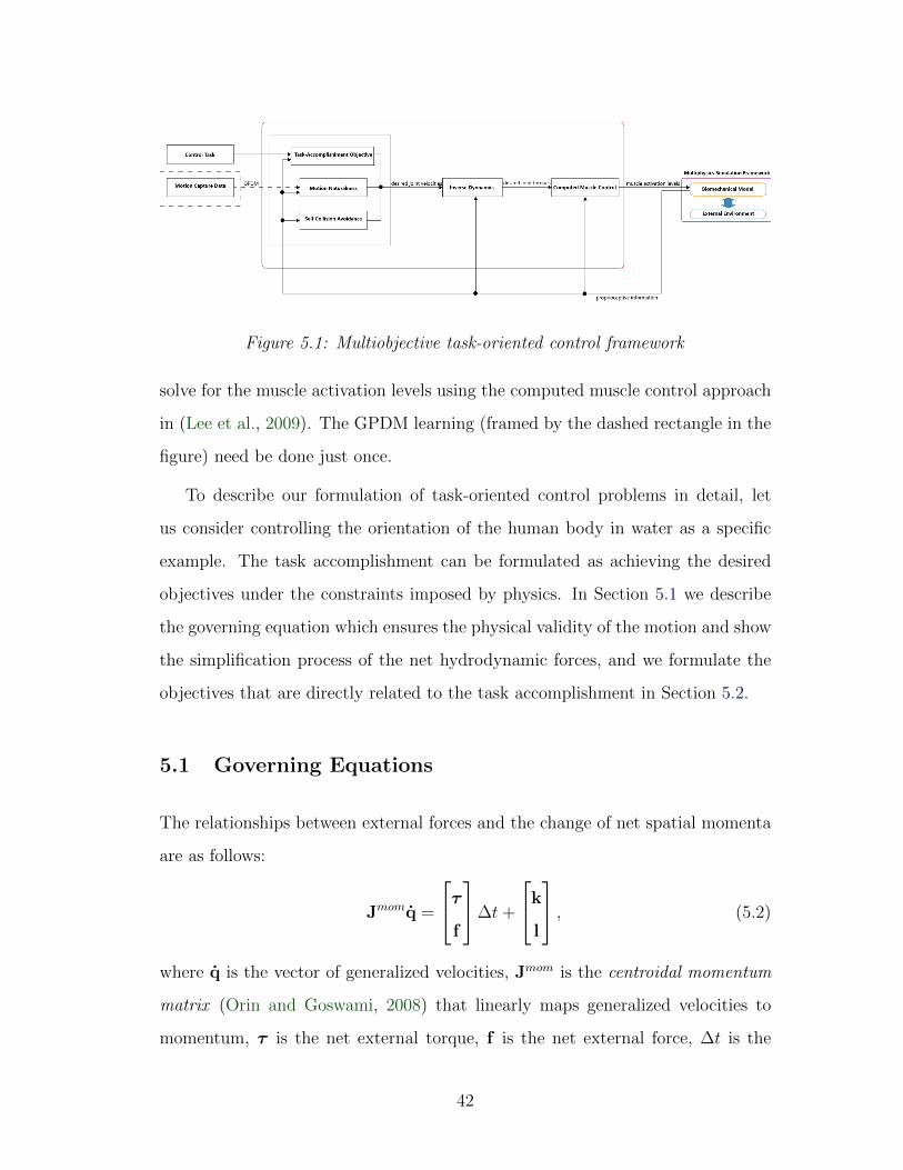
Figure 5.1: Multiobjective task-oriented control framework
solve for the muscle activation levels using the computed muscle control approach
in (Lee et al., 2009). The GPDM learning (framed by the dashed rectangle in the
figure) need be done just once.
To describe our formulation of task-oriented control problems in detail, let
us consider controlling the orientation of the human body in water as a specific
example. The task accomplishment can be formulated as achieving the desired
objectives under the constraints imposed by physics. In Section 5.1 we describe
the governing equation which ensures the physical validity of the motion and show
the simplification process of the net hydrodynamic forces, and we formulate the
objectives that are directly related to the task accomplishment in Section 5.2.
5.1 Governing Equations
The relationships between external forces and the change of net spatial momenta
are as follows:
Jmomq =
τf
∆t+
k
l
, (5.2)
where q is the vector of generalized velocities, Jmom is the centroidal momentum
matrix (Orin and Goswami, 2008) that linearly maps generalized velocities to
momentum, τ is the net external torque, f is the net external force, ∆t is the
42
time step, l is linear momentum, k is the centroidal angular momentum, which
is the aggregate angular momentum of the human body projected at its center of
mass (CoM).
For a human body inside water, f comprises gravity, buoyancy, and the net hy-
drodynamic force. Since gravity and buoyancy approximately cancel one another,
f is mainly the net hydrodynamic force. As seen in (3.12), for each small area of
the human body, the hydrodynamic force approximately scales as the square of the
relative velocity of that area with respect to the fluid. We divide the human body
into m parts and assume that we can use a quadratic relationship to approximate
the net hydrodynamic force for each part. In more detail, for part i, we simply use
the face centers of the skin geometry triangles for that part as sampling points,
and use fi, vsi and vfi to denote the net hydrodynamic force, mean velocity of
the skin, and mean velocity of the fluid computed from those sampling points,
respectively. We also assume that the following quadratic relationship suffices to
represent the net hydrodynamic force:
fi = ci||vsi − vfi ||2, (5.3)
where ci is the coefficient vector. We can compute ci for each part given fi, vsi , and
vfi . For the purposes of control, we wish to represent the net hydrodynamic force
fi and the corresponding net torque τ i as functions of the generalized velocities.
We do so by finding a point ri on part i that satisfies v(ri) = vsi and ri × fi = τ i
in the least-squares sense, where v(ri) is the velocity at a point ri. For simplicity,
we use vbi , interpreted as the velocity of a mean point for the ith body part, to
denote v(ri). Then we have
fi = ci||vbi − vfi ||2. (5.4)
To formulate (5.2) as a quadratic programming problem, we further simplify this
as a linear equation using a Taylor expansion around vsi on the right hand side of
43
(5.4):
||vbi − vfi ||2 ≈ ||vsi − vfi ||2 + 2(vsi − vfi
)T (Jveli q− vfi
)= di + eTi q, (5.5)
where Jveli is the Jacobian matrix that linearly maps q to vbi , and
di = ||vsi − vfi ||2 − 2(vsi − vfi
)Tvfi , (5.6)
eTi = 2Jveli
T(vsi − vfi
). (5.7)
Substituting (5.5) into (5.4) yieldsτf
=
∑ τ i∑fi
=∑ri × ci
ci
(di + eTi q)
(5.8)
We substitute this into (5.2) to obtain a linear equation for q:
Aq = b, (5.9)
where
A = Jmom −∑ri × ci
ci
eTi ∆t (5.10)
and
b =∑ri × ci
ci
di∆t+
k
l
. (5.11)
The governing equation (5.2) should be used as a constraint in our control problem.
We use a quadratic objective function to treat it as a soft constraint Egov =
||Aq− b||2.
Next, we will formulate the objectives that are directly related to task accom-
plishment.
44
5.2 Task-Related Objectives
In order to make the human body rotate efficiently, we want the torque along
the desired rotation axis to be as large as possible, so we use a linear objective
function
Erot = −ωTτ (5.12)
to achieve this, where ω is the desired rotation axis. This Erot is very important
in order to generate efficient rotational motion. When the human body reaches
some pose limit, it is possible that the body may rotate in the reverse direction,
this linear term is very effective in mitigating this undesired effect. In general,
humans tend to twist their trunk to guide the rotation of their body, so we use
Jtrkvelq = vtrkdes (5.13)
as a soft constraint to achieve the trunk twisting effect; i.e.,
Etrk = ||Jtrkvelq− vtrkdes||2. (5.14)
For the orientation control problem, vtrkdes is the desired trunk angular velocity and
Jtrkvel is the Jacobian matrix that linearly maps q to the trunk angular velocity.
We use the orientation and velocity of the first thoracic vertebra to represent the
trunk orientation and velocity. The desired angular velocity is computed using a
feedback rule:
atrkdes = kp log(R−1desR
)− kdvtrk (5.15)
vtrkdes = vtrk + atrkdes∆t, (5.16)
where Rdes,R ∈ SO(3) are the desired trunk orientation and the current trunk
orientation respectively, kp and kd are proportional and derivative feedback gains,
respectively, and vtrk is the current angular velocity of the trunk.
45
In summary, the orientation control objective function for task accomplishment
can be formulated as a weighted combination of the sub-objective functions; i.e.,
Eorient = Egov + wtrkEtrk + wrotErot
= ||Aq− b||2 + wtrk||Jtrkvelq− vtrkdes||2
− wrotωT∑
ri × ci(di + eTi q
)(5.17)
This is a quadratic function of q. Note that ri, ci, di, and ei are updated per
frame. We set wtrk = 1 and wrot = 1000 for all the results presented in this thesis.
5.3 Naturalness
Although we can achieve orientation control by minimizing Eorient, the resulting
motion might be very unnatural (see Chapter 6). The motion unnaturalness may
originate from multiple sources, but there are two common cases among them.
First, the human body may run into some unnatural pose, even though the joint
limits are satisfied. Second, the motion may not be fluid even though the pose
itself is natural; e.g., the human body is stuck in some pose for a while. We could
easily run into these cases if we simply optimize Eorient alone without a term
that encourages natural poses in Eorient and it is also very likely to get stuck in
some solution temporarily because of the temporal locality of our optimization
scheme. In order to handle these cases, we use the GPDM, which encodes both
pose naturalness and temporal dynamics information of the motion, to provide a
preferred solution qnat and define an objective function
Enat = ||q− qnat||2. (5.18)
46
To obtain qnat, we first solve for a latent point xnat that defines the natural pose
(or velocity) by minimizing
Enat (xt+1) = Exorient + wpriorEprior
+ wsmoothEsmooth + wconfidEconfid
= Eorient (q (µY (xt+1)))− wprior ln p(X(∗)|Γ
)+ wsmooth||µY (xt+1)− µY (xt)||2
+ wconfidσ2Y (xt+1). (5.19)
This objective function is defined similarly to (Levine et al., 2012), which uses
the GP to map the joint space to latent space and defines the motion quality
term using a latent space motion prior, smoothness, as well as the prediction
variance of the reconstruction GP. In detail, µY (x) is the mean of the GP for
pose reconstruction as a function of the latent space position x, Γ is the learned
GPDM model parameters. X(∗) is the latent trajectory. In our application, we
use three adjacent latent points as X(∗); i.e., X(∗) = [xt−1,xt,xt+1]T . σ2Y (x) is
the prediction variance. In this equation, Exorient = Eorient (q (µY (xt+1))) prefers
solutions that are consistent with the orientation control objective, and Eprior =
− ln p(X(∗)|Γ
)encourages output motion to be close to the training data. Another
big advantage of this Eprior is that it makes the motion fluid, preventing the
human body from becoming stuck in some pose due to local optimality or a joint
limit. Esmooth = ||µY (xt+1) − µY (xt)||2 measures the smoothness of the motion
in feature space, Econfid = σ2Y (xt+1) measures the confidence of the reconstructed
pose from the latent position and prefers natural poses that are closer to the
training data. Although Eprior partially overlaps with Esmooth and Econfid in terms
of functionality, we found that having Esmooth and Econfid explicitly in the objective
function results in easier and more intuitive control of different sub-objectives.
The exact definition of µY (x), p(X(∗)|Γ
), and σ2
Y (x) can be found in (Wang et al.,
2008). Due to a nice property of the GP, we can efficiently compute ∂Enat/∂xt+1
47
analytically. With this partial derivative, we can efficiently solve a nonlinear
optimization problem; i.e.,
xnat = arg minxt+1
Enat (xt+1) (5.20)
to obtain a latent point xnat that defines the natural pose (or velocity). Exper-
iments show that we can generally find a decent suboptimal solution. Then we
can compute qnat from µY (xnat). In our application, we use joint angles (pose)
as the feature vector y for the GPDM and compute q (µY (xt+1)) in (5.19) as well
as qnat using the numerical pose difference. We can initialize x0 by minimizing
||q0 − µY (x)||.
After we impose Enat, it is possible that this sub-objective will conflict with
Eorient, which may result in reverse rotation; however, the existence of the linear
term Erot will largely mitigate this effect. In practice, we always achieve the
desired orientation after several trials.
In our application, to make the latent space more powerful and flexible in
representing motion space from limited training data, we train four GPDM models
for the respective limbs independently with a connectivity prior as suggested in
(Levine et al., 2012). We fill in Exorient with latent points that are defined within
these GPDM models and leave unmodified the joints (e.g., joints that correspond
to the trunk bones) that are not specified by any latent space. We define the
other sub-objectives to be the summation of the limb GPDM sub-objectives; i.e.,
Eprior =∑4
j=1Ejprior, Esmooth =
∑4j=1E
jsmooth and Econfid =
∑4j=1 E
jconfid. Note
that even with all of these, minimizing Enat by itself does not result in motion that
achieves the desired orientation, although we have the orientation sub-objective
term in (5.19). In fact, the solved motion is quite inefficient in orientation control
due to the limited training data and the inadequate capacity of the GPDM to
handle large, heterogeneous datasets. However, it serves very well to make the
resulting motion natural. For the experimental results we present in this thesis,
48
we set wprior = 5 · 10−7, wsmooth = 0.5, and wconfid = 5.
5.4 Collision Constraints
Self-collision avoidance is handled via soft constraints as in (Ho et al., 2010).
Collision constraints can be applied through the following equation:
Cq = vcdes. (5.21)
Row i of this equation is
nTi(JC1i − JC2
i
)q = vdesi , (5.22)
where ni is the unit vector computed from the ith closest point pair on the colliding
bodies, JC1i and JC2
i are the Jacobian matrices that map the generalized velocities
to the velocities of the closest point pair, and vdesi is the desired relative velocity
of the point pair in the ni direction. We use the exponential of the penetration
depth to compute vdesi . To detect self-collision, we bound each body segment by
a capsule. We also treat the collision constraints as soft constraints; i.e.,
Ecld = ||Cq− vcdes||2. (5.23)
5.5 Solution
We substitute (5.17), (5.19), and (5.23) into (5.1) with Etask = Eorient, and solve
the quadratic programming problem
qdes = arg minqE (q) . (5.24)
After solving for qdes, we perform inverse dynamics to compute the necessary
torques to achieve qdes, and then solve for muscle activation levels using the muscle
control approach in (Lee et al., 2009). For all our experimental results, we set
49
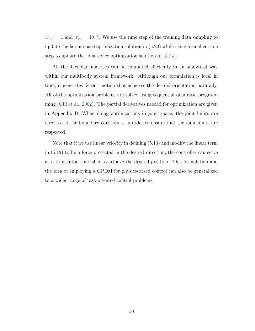
wnat = 1 and wcld = 10−4. We use the time step of the training data sampling to
update the latent space optimization solution in (5.20) while using a smaller time
step to update the joint space optimization solution in (5.24).
All the Jacobian matrices can be computed efficiently in an analytical way
within our multibody system framework. Although our formulation is local in
time, it generates decent motion that achieves the desired orientation naturally.
All of the optimization problems are solved using sequential quadratic program-
ming (Gill et al., 2002). The partial derivatives needed for optimization are given
in Appendix D. When doing optimizations in joint space, the joint limits are
used to set the boundary constraints in order to ensure that the joint limits are
respected.
Note that if we use linear velocity in defining (5.13) and modify the linear term
in (5.12) to be a force projected in the desired direction, the controller can serve
as a translation controller to achieve the desired position. This formulation and
the idea of employing a GPDM for physics-based control can also be generalized
to a wider range of task-oriented control problems.
50
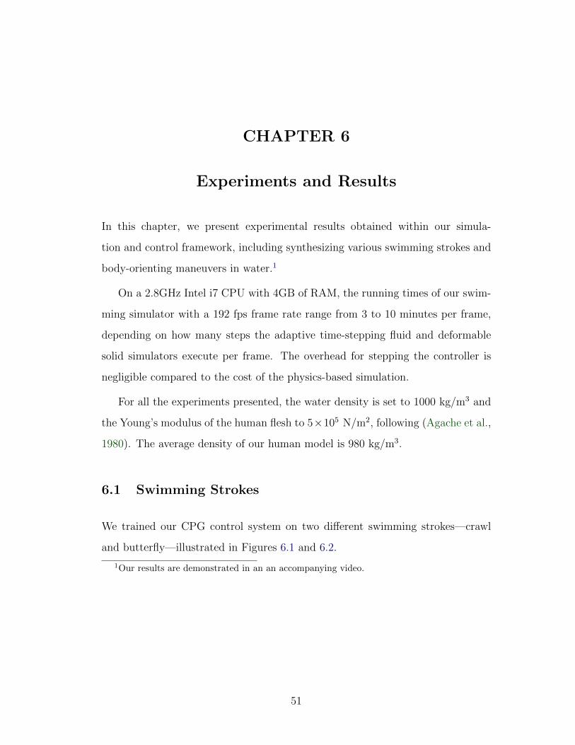
CHAPTER 6
Experiments and Results
In this chapter, we present experimental results obtained within our simula-
tion and control framework, including synthesizing various swimming strokes and
body-orienting maneuvers in water.1
On a 2.8GHz Intel i7 CPU with 4GB of RAM, the running times of our swim-
ming simulator with a 192 fps frame rate range from 3 to 10 minutes per frame,
depending on how many steps the adaptive time-stepping fluid and deformable
solid simulators execute per frame. The overhead for stepping the controller is
negligible compared to the cost of the physics-based simulation.
For all the experiments presented, the water density is set to 1000 kg/m3 and
the Young’s modulus of the human flesh to 5×10⁵ N/m2, following (Agache et al.,
1980). The average density of our human model is 980 kg/m3.
6.1 Swimming Strokes
We trained our CPG control system on two different swimming strokes—crawl
and butterfly—illustrated in Figures 6.1 and 6.2.
1Our results are demonstrated in an an accompanying video.
51
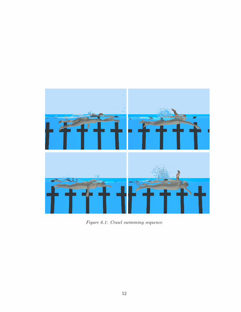
Figure 6.1: Crawl swimming sequence
52
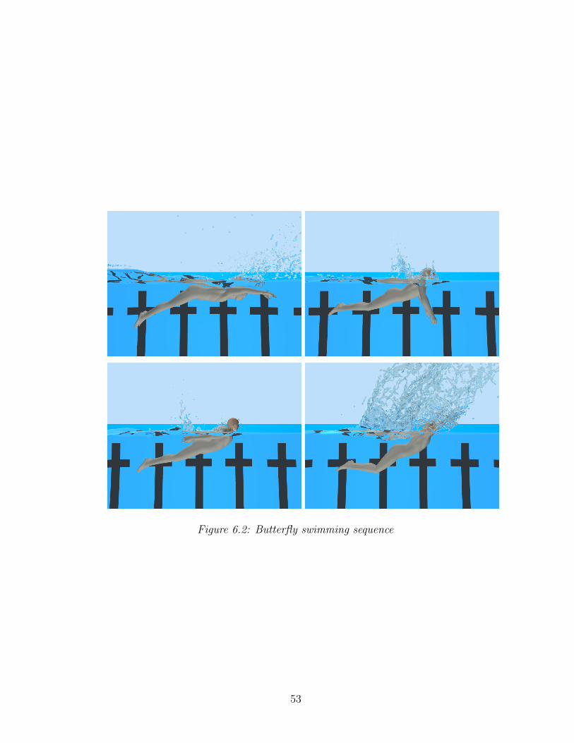
Figure 6.2: Butterfly swimming sequence
53
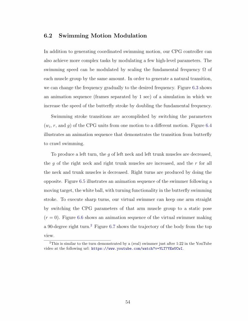
6.2 Swimming Motion Modulation
In addition to generating coordinated swimming motion, our CPG controller can
also achieve more complex tasks by modulating a few high-level parameters. The
swimming speed can be modulated by scaling the fundamental frequency Ω of
each muscle group by the same amount. In order to generate a natural transition,
we can change the frequency gradually to the desired frequency. Figure 6.3 shows
an animation sequence (frames separated by 1 sec) of a simulation in which we
increase the speed of the butterfly stroke by doubling the fundamental frequency.
Swimming stroke transitions are accomplished by switching the parameters
(wi, r, and g) of the CPG units from one motion to a different motion. Figure 6.4
illustrates an animation sequence that demonstrates the transition from butterfly
to crawl swimming.
To produce a left turn, the g of left neck and left trunk muscles are decreased,
the g of the right neck and right trunk muscles are increased, and the r for all
the neck and trunk muscles is decreased. Right turns are produced by doing the
opposite. Figure 6.5 illustrates an animation sequence of the swimmer following a
moving target, the white ball, with turning functionality in the butterfly swimming
stroke. To execute sharp turns, our virtual swimmer can keep one arm straight
by switching the CPG parameters of that arm muscle group to a static pose
(r = 0). Figure 6.6 shows an animation sequence of the virtual swimmer making
a 90-degree right turn.2 Figure 6.7 shows the trajectory of the body from the top
view.
2This is similar to the turn demonstrated by a (real) swimmer just after 1:22 in the YouTubevideo at the following url: https://www.youtube.com/watch?v=YLT7YEwUCwI.
54
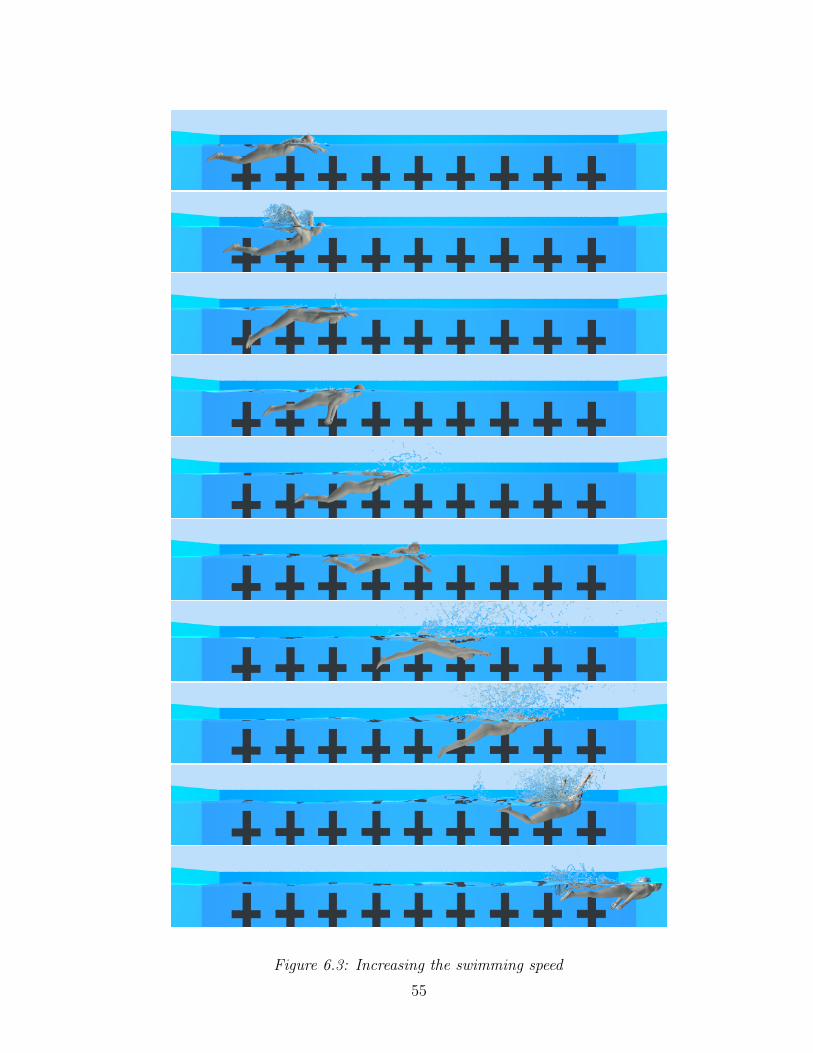
Figure 6.3: Increasing the swimming speed
55
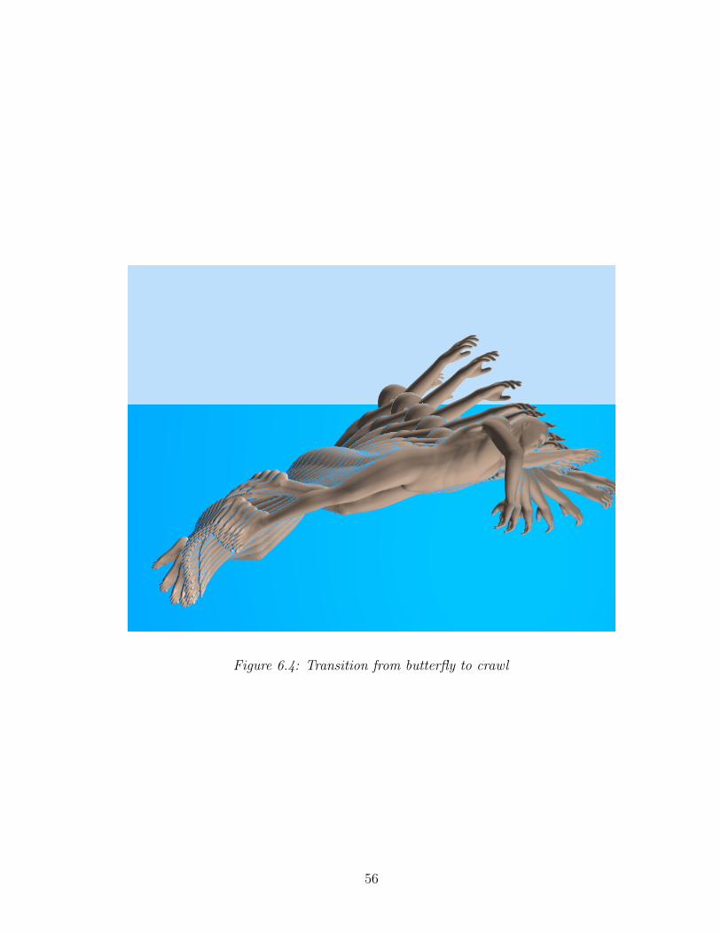
Figure 6.4: Transition from butterfly to crawl
56
Figure 6.5: Turning to follow a moving target white ball using the butterfly
swimming stroke
57
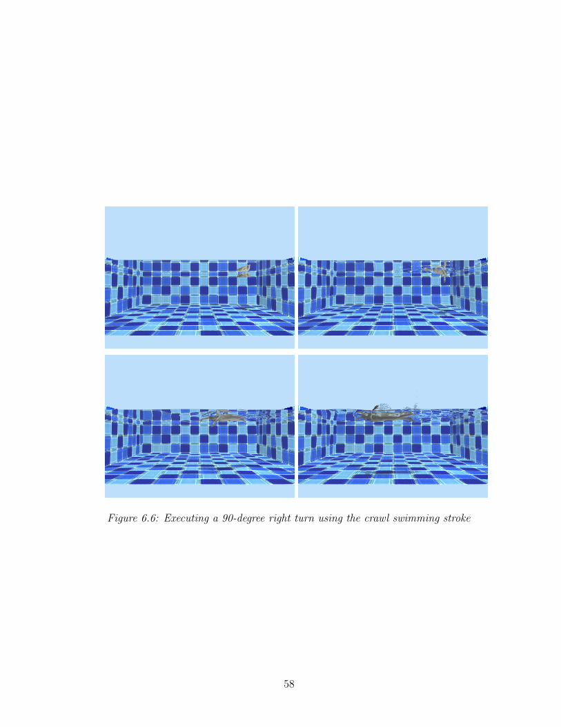
Figure 6.6: Executing a 90-degree right turn using the crawl swimming stroke
58
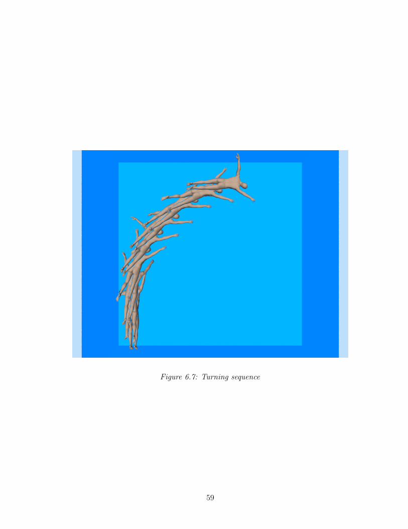
Figure 6.7: Turning sequence
59
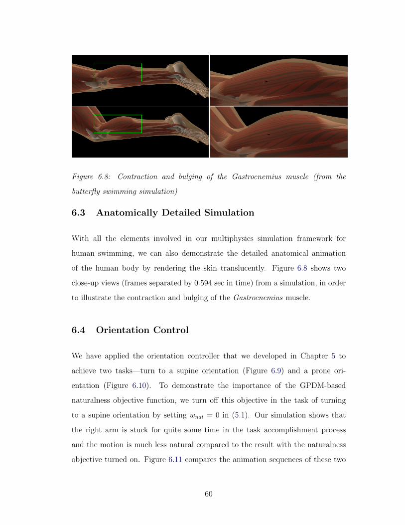
Figure 6.8: Contraction and bulging of the Gastrocnemius muscle (from the
butterfly swimming simulation)
6.3 Anatomically Detailed Simulation
With all the elements involved in our multiphysics simulation framework for
human swimming, we can also demonstrate the detailed anatomical animation
of the human body by rendering the skin translucently. Figure 6.8 shows two
close-up views (frames separated by 0.594 sec in time) from a simulation, in order
to illustrate the contraction and bulging of the Gastrocnemius muscle.
6.4 Orientation Control
We have applied the orientation controller that we developed in Chapter 5 to
achieve two tasks—turn to a supine orientation (Figure 6.9) and a prone ori-
entation (Figure 6.10). To demonstrate the importance of the GPDM-based
naturalness objective function, we turn off this objective in the task of turning
to a supine orientation by setting wnat = 0 in (5.1). Our simulation shows that
the right arm is stuck for quite some time in the task accomplishment process
and the motion is much less natural compared to the result with the naturalness
objective turned on. Figure 6.11 compares the animation sequences of these two
60
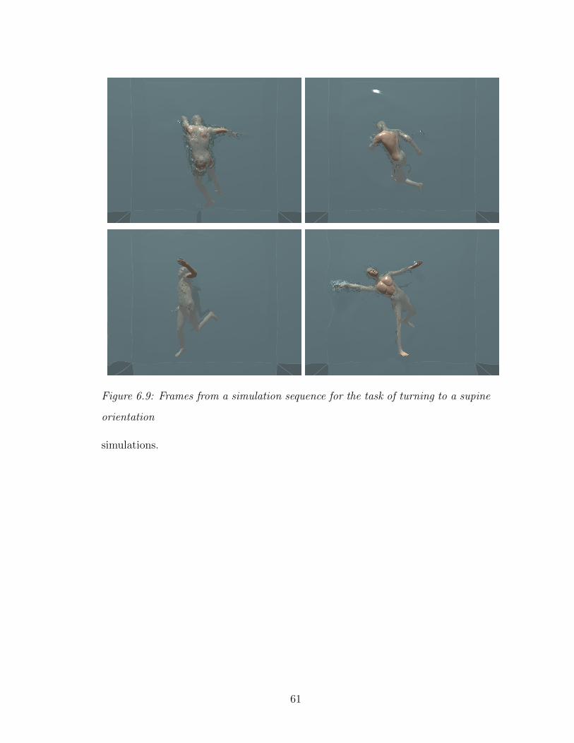
Figure 6.9: Frames from a simulation sequence for the task of turning to a supine
orientation
simulations.
61
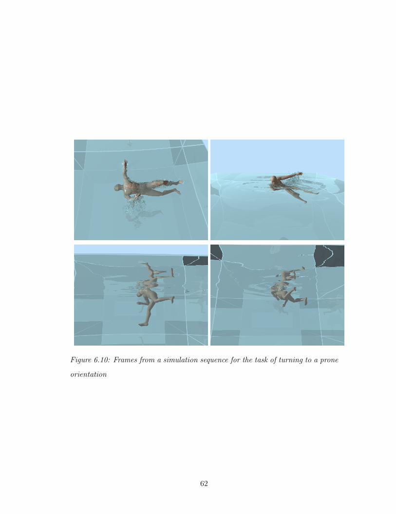
Figure 6.10: Frames from a simulation sequence for the task of turning to a prone
orientation
62
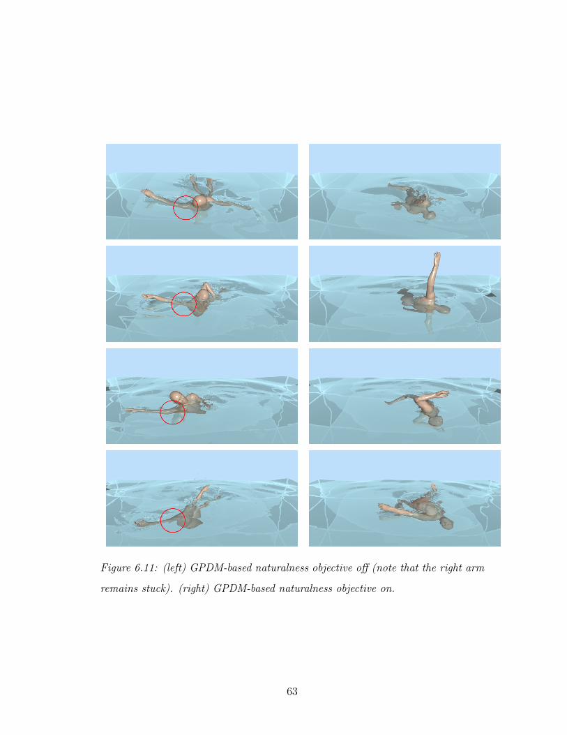
Figure 6.11: (left) GPDM-based naturalness objective off (note that the right arm
remains stuck). (right) GPDM-based naturalness objective on.
63
CHAPTER 7
Discussion
Our interleaved approach to coupling fluid, flesh, and skeletal components pro-
vides us flexibility and versatility in constructing our simulation and control
framework from different algorithmic building blocks and simulation algorithms.
However, interleaved coupling reflects a conscious compromise in traits such as
stability, accuracy, and performance potential. A more tightly-coupled system
with deformable, fluid, and rigid components would, in theory, enable implicit
time-integration techniques that would achieve stable simulation while tolerating
larger time steps. In contrast, we take the most time-step-restrictive of the phases
involved (generally the fluid) and use it to dictate the time-step for the entire
interleaved simulation cycle. As controllers and modular simulation components
mature, a tightly-coupled multiphysics-control system would certainly be appro-
priate.
Although the interleaved coupling of skeleton, flesh, and fluid provide flexibility
and ease in constructing the simulation framework, they also compromise stability,
accuracy, and performance. We sacrifice accuracy for stability in our fluid-skin
coupling by using the reliable velocity field rather than the unreliable pressure
field to compute hydrodynamic forces on the body. To employ pressure, we
would need a better fluid solver and/or a better coupling method. For the flesh-
skeleton coupling, we sacrifice performance for stability and accuracy. In order to
produce stable flesh-skeleton simulation under large environmental perturbation
(e.g., ground collision), we would have to take very small time steps. This could
64
be aided by computing a Jacobian matrix, which represents the flesh force change
acting on the bones with respect to the skeleton pose change, and use it in an
implicit integration of the multibody dynamics system.
Our combined use of PLS muscle forces and forces stemming from the volu-
metric flesh simulation has an interesting consequence. The mechanical response
of the skeleton to a specific pose includes force components arising from both the
PLS model and the volumetric simulation. For example, reactive forces act on
the bones as the body pose causes stretching or compression of the flesh. Such a
response serves a similar purpose as the passive component of PLS muscles. In
addition, since our flesh simulation incorporates active musculature, the contrac-
tion of such volumetric muscles will transmit forces to their attached bones. In
an ideal setting, the volumetric simulation would capture the entirety of forces
due to flesh elasticity and muscle contraction alike. However, obtaining accurate
muscle forces exclusively from the volumetric simulation requires a great degree
of modeling accuracy, including detailed geometric and material descriptions for
tendons and connective tissues. This is a significantly higher standard of modeling
detail and accuracy than would be necessary for recreating natural looking flesh
deformations, where the accuracy of deep muscle forces is not a crucial factor. On
the other hand, while the PLS approximation does not provide information on
volumetric deformation, it is capable of reproducing stable and biomechanically
faithful muscle forces and torques. Our approach has been to include both
sources of force, and use each to compensate for inaccuracies in the other. For
example, in the absence of tendon models in the volumetric flesh simulation,
the effect of muscle contraction on bones is greatly diluted, and spread out over
a broader area than the actual point of attachment; this is compensated by
relying on the PLS model to contribute the bulk of the articulatory forces. On
the other hand, the transfer of forces acting on the skin to the bones via the
elastic flesh relies almost exclusively on the volumetric simulation. Ultimately, we
65
treat the combined PLS/volumetric simulation system as a combined anatomical
approximation whose parameters are adapted to produce realistic simulation.
We will next report on an additional set of experiments aimed at assessing the
importance of various simulation/control components of our framework relative
to alternative approaches.
7.1 CPG Control vs. Splines
On a fundamental level, we advocate CPG-based locomotion control, since the
CPG is a principled low-level motor control mechanism from a biological per-
spective. However, spline-based animation methods have traditionally been more
familiar to graphics practitioners. In fact, as discussed in Section 4.1, we initially
use cubic B-splines to approximate the CPG training data. As a simple alternative
to the CPG dynamical model, our continuous spline approximations may be
repeated in time to produce periodic muscle signals to drive our virtual swimmer.
The accompanying video includes a comparison of our CPG-controlled swimming
against spline-controlled swimming. Although the results look qualitatively sim-
ilar for any particular swimming stroke in steady state, the spline technique
is noticeably choppier than the CPG technique due to discontinuities in the
derivatives of the periodic spline functions across cycles, whereas the muscle
control signals generated by our CPGs are always C1 smooth. Moreover, to
switch from one swimming stroke to another, the spline-based controller would
have to transition carefully between numerous periodic spline functions, one per
muscle. By contrast, our CPG muscle controllers can effect smooth transitions
and control swimming speed by simply switching and/or modifying the values of
a few parameters.
66
7.2 Muscle Control vs. Joint Torques
On a fundamental level, we advocate muscle-based control as contractile muscles
are the principled skeletal actuation mechanism from a biological perspective.
However, joint-torque animation control methods have traditionally been more
familiar to graphics practitioners. Since skeletal muscle forces, through (bone)
moment arms, eventually produce torques at rotational joints in the skeleton (but
see (Lee and Terzopoulos, 2008)), we can in principle achieve similar animation re-
sults through equivalent joint-torque-driven simulation. The accompanying video
includes a comparison of our muscle-actuated simulation against both inverse-
dynamic (ID) and PD joint-torque actuated simulation. In the case of swimming,
we obtained plausible results using joint-torque actuation, but it was necessary to
set high gains for the PD joint-torque controllers accompanied with an order-of-
magnitude smaller numerical time-step compared to the muscle-based approach.
Moreover, a further advantage of the latter is that modifying the parameters of
contractile muscles situated in anatomically accurate positions is the natural way
to create nuanced biological motion patterns, including pathological ones (Wang
et al., 2012), as well as of naturally effecting realistic flesh deformations (Lee et al.,
2009).
7.3 Flesh Simulation vs. Procedural Skinning
On a fundamental level, we advocate volumetric soft-tissue simulation as this is the
principled fleshing approach from a biological perspective. However, procedural
skinning techniques have traditionally been more familiar to graphics practition-
ers. The accompanying video includes a comparison of our deformable flesh sim-
ulation against a state-of-the-art dual-quaternion skinning method (Kavan et al.,
2008) with bounded biharmonic weights (Jacobson et al., 2011). The volumetric
flesh simulation and procedural skinning result in similar swimming performances.
67
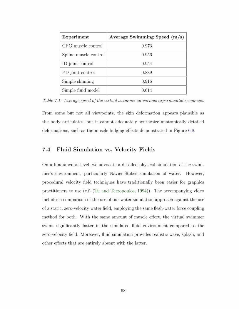
Experiment Average Swimming Speed (m/s)
CPG muscle control 0.973
Spline muscle control 0.956
ID joint control 0.954
PD joint control 0.889
Simple skinning 0.916
Simple fluid model 0.614
Table 7.1: Average speed of the virtual swimmer in various experimental scenarios.
From some but not all viewpoints, the skin deformation appears plausible as
the body articulates, but it cannot adequately synthesize anatomically detailed
deformations, such as the muscle bulging effects demonstrated in Figure 6.8.
7.4 Fluid Simulation vs. Velocity Fields
On a fundamental level, we advocate a detailed physical simulation of the swim-
mer’s environment, particularly Navier-Stokes simulation of water. However,
procedural velocity field techniques have traditionally been easier for graphics
practitioners to use (c.f. (Tu and Terzopoulos, 1994)). The accompanying video
includes a comparison of the use of our water simulation approach against the use
of a static, zero-velocity water field, employing the same flesh-water force coupling
method for both. With the same amount of muscle effort, the virtual swimmer
swims significantly faster in the simulated fluid environment compared to the
zero-velocity field. Moreover, fluid simulation provides realistic wave, splash, and
other effects that are entirely absent with the latter.
68
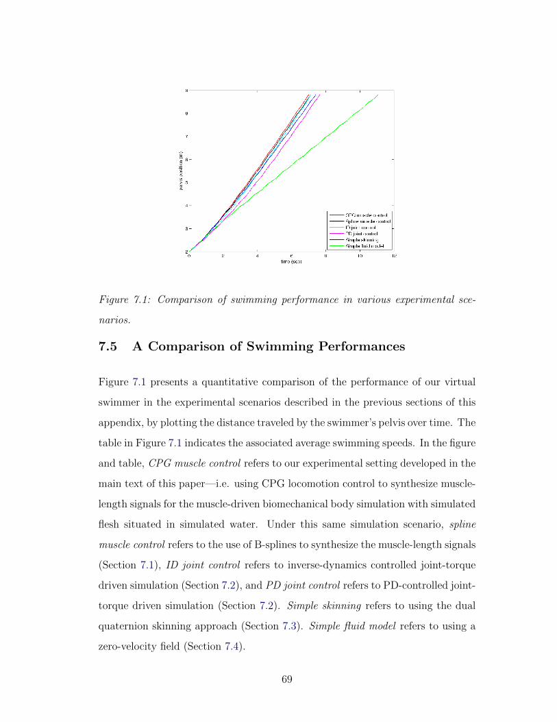
Figure 7.1: Comparison of swimming performance in various experimental sce-
narios.
7.5 A Comparison of Swimming Performances
Figure 7.1 presents a quantitative comparison of the performance of our virtual
swimmer in the experimental scenarios described in the previous sections of this
appendix, by plotting the distance traveled by the swimmer’s pelvis over time. The
table in Figure 7.1 indicates the associated average swimming speeds. In the figure
and table, CPG muscle control refers to our experimental setting developed in the
main text of this paper—i.e. using CPG locomotion control to synthesize muscle-
length signals for the muscle-driven biomechanical body simulation with simulated
flesh situated in simulated water. Under this same simulation scenario, spline
muscle control refers to the use of B-splines to synthesize the muscle-length signals
(Section 7.1), ID joint control refers to inverse-dynamics controlled joint-torque
driven simulation (Section 7.2), and PD joint control refers to PD-controlled joint-
torque driven simulation (Section 7.2). Simple skinning refers to using the dual
quaternion skinning approach (Section 7.3). Simple fluid model refers to using a
zero-velocity field (Section 7.4).
69

The figure and table reveal that the virtual swimmer swims most efficiently in
our original experimental scenario. The swimmer can achieve similar swimming
performances in the other experimental settings, except when the simulated fluid
model is replaced by a zero-velocity field, which result in significantly lower
efficiency.
70
CHAPTER 8
Conclusion
8.1 Contributions of the Thesis
In summary, the primary contributions of the human animation research reported
in this dissertation are as follows:
• We have introduced a multiphysics simulation and control framework
within whose scope is the realistic animation of a sophisticated autonomous
human model that is capable of controlled swimming and underwater orien-
tation control.
• We have developed a comprehensive biomechanical model of the hu-
man body, which includes 103 rigid bones (comprising 163 articular degrees
of freedom) simulated as an articulated, multibody dynamical system that
is driven by 823 muscles modeled as piecewise uniaxial Hill-type contractile
actuators, plus a muscle and passive flesh simulation via an efficient volumet-
ric finite element model of quasi-incompressible elastic material augmented
with active (contractile) muscle terms, as well as the appropriate two-way
coupling between the articulated skeleton and deformable flesh.
• With regard to the control of the biomechanical human model to syn-
thesize complex, coordinated movements in water, we developed a Central
Pattern Generator (CPG) based controller that generates muscle activation
signals to induce appropriately coordinated muscle contractions. We also
71
developed a multiobjective optimization based control method that enables
our biomechanical human model to accomplish nonperiodic, task-oriented
motions in water while encouraging motion naturalness and avoiding self-
collisions.
8.2 Future Work
Contemplating how people learn to swim, we are inspired to further investi-
gate this topic in our future work. Humans learn to swim by first learning the
movement of the limbs, perhaps by mimicking swimming demonstrations. This
corresponds to the supervised learning process of our CPG system. After attaining
command of the kinematic pattern of a swimming stroke, one can improve one’s
swimming skill through practice. This can be treated as an optimization process.
As seen in the video, currently the motions of our swimmer are not very efficient,
but we can try to optimize the learned parameters of our CPG system in order
to improve efficiency. Generally speaking, CPG models offer a good substrate
for automated learning and optimization algorithms. Studying how the swimmer
responds to perturbations will be another interesting research direction. We can
potentially simulate how a human should perform swimming in a torrential flow.
In the aquatic environment, we do not deal with balance, and losing bal-
ance does not cause serious problems for underwater motion control in a calm
water environment, since buoyancy approximately cancels gravity and humans
can efficiently control their limbs to generate proper drag forces, thus making
their motions controllable. Under large perturbations, however, we are forced to
confront balance in order to produce controllable motion. Balance is also a very
troublesome issue when controlling terrestrial motion. It will not suffice to simply
apply our CPG controller to walking and running motions as we would need to
develop a more sophisticated feedback scheme to handle the balance problem.
72
This will be another interesting avenue for future work. Real world motion may
be a superimposition of locomotion and voluntary movements; e.g., waving hands
while walking. Combining our CPG controller with other controllers, such as the
neuromuscular controller developed in (Lee and Terzopoulos, 2006), may be a
viable approach to dealing with a broader variety of motor tasks.
For our orientation controller, the motion efficiency and naturalness are still
not up to the standards of real human motion. Motion efficiency can be improved
by formulating a better objective function for changing orientation, as well as
a better approximation of the net hydrodynamic force effect. GP approaches
have shown promise in synthesising natural kinematic human motion, and another
possible direction for future work is finding a better way to couple the task control
with the GP to improve the motion naturalness while not losing motion efficiency.
Energy efficiency, which is an important principle for human motion, is not
considered in our proposed controllers. Since we cannot afford global spatiotem-
poral optimization for our complex system, it is very challenging to apply the
energy efficiency principle to the system directly. A possible solution is to obtain
an energy-efficient controller from a simplified system and then refine it for use in
the actual simulation framework, another possible avenue for future work.
73
APPENDIX A
Rendering
We use the open-source POV-Ray software to render our simulation results. The
geometries of the skin, muscles, and skeleton are embedded into the hexahedra
of the embedding volume. This embedding framework preserves high resolution
geometry for rendering. The water is treated as an isosurface object. The particle
level set method provides a level set representation for the surface of the water,
however, this level set representation cannot generate rich splashing effects unless
the fluid is simulated at very high resolution. To make our fluid simulation
affordable and the rendering result visually appealing, we make use of a byproduct
of the fluid simulation, the removed negative particles, to render splashes.
We reconstruct a smooth surface representation from the removed negative
particles using the approach in (Yu and Turk, 2010), which formulates the implicit
surface representation as a sum of anisotropic smoothing kernels. The direction
of anisotropy at a particle is determined by performing Principal Components
Analysis (PCA) over the neighboring particles. Since these anisotropic smoothing
kernels capture the local particle distributions more accurately, this method has
advantages in representing smooth surfaces, thin streams, and sharp fluid features.
It is also fast and easy to implement.
The surface is defined as an isosurface of a scalar field
φ (x) =∑j
mj
ρjW (x− xj,Gj), (A.1)
where x is a location in space, mj is the particle mass, and W is an anisotropic
74
smoothing kernel of the form
W (r,G) = σ‖G‖P (‖Gr‖) . (A.2)
Here, r is a radial vector, G is a linear transformation that rotates and stretches
r, σ is a scaling factor, which we set to − 31565π
, and P is a symmetric decaying
spline with finite support, which we simply define P as
P (x) =
(1− x)3 if 0 ≤ x ≤ 1
0 otherwise.
(A.3)
The density ρi in (A.1) is interpolated by a sum of the weighted contributions of
nearby particle masses mj:
ρi =∑j
mjW (xj − xi,Gj). (A.4)
The key idea of this method is to associate an anisotropic matrix Gj with
each particle j so that Gj more accurately represents the neighborhood density
distribution. In order to determine G, we apply the weighted version of PCA
(WPCA) that is proposed in (Koren and Carmel, 2003) to the neighborhood
particle positions. Specifically, WPCA begins by computing a weighted mean of
data points:
xwi =∑j
wijxj/∑j
wij. (A.5)
Next, it constructs a weighted covariance matrix C with a zero empirical mean:
Ci =∑j
wij (xj − xwi ) (xj − xwi )T/∑j
wij. (A.6)
The function wij is an isotropic weighting function with respect to particle i and
j with support ri:
wij =
1− (‖xi − xj‖/ri)3 if ‖xi − xj‖ < ri,
0 otherwise.
(A.7)
75
With the finite support of wij, the computation is confined to the neighborhood
particles within the radius ri. To determine efficiently the particles that are within
some radius of each particle, we build a balanced k-d tree for all the particles ahead
of the other computations.
Then we perform an eigendecomposition on C:
C = RΣRT , (A.8)
where R is a rotation matrix with principal axes as column vectors, and Σ is a
diagonal matrix with eigenvalues σ1 ≥ · · · ≥ σd:
Σ = diag (σ1, · · · , σd) . (A.9)
In order to deal with singular matrices and prevent extreme deformations, we
check if σ1 ≥ krσd with a suitable positive constant kr > 1. This condition is true
when the largest variance in one principal axis is much bigger than the variance
in another axis. In this case, we modify C so that the ratio between any two
eigenvalues is within kr. When the number of particles in the neighborhood is too
small, we reset W to a spherical shape by setting G = knI in order to avoid poor
particle deformations for nearly isolated particles. We also multiply C by scaling
factor ks such that ‖ksC‖ ≈ 1 for the associated particle inside the fluid volume.
Σ =
ksdiag (σ1, σ2, · · · , σd) if N > Nε,
knI otherwise,
(A.10)
where σk = max (σk, σ1/kr). In our application, we use kr = 4, ks = 1400,
kn = 0.2, and Nε = 25.
Gi =1
hiRΣ−1RT . (A.11)
We use hi = 0.04 and ri = 2hi.
76
APPENDIX B
Improved Flesh-Bone Coupling
The key idea in improving flesh-bone coupling is to provide the Jacobian matrix
of the attachment spring forces fc with respect to the joint coordinates q; i.e.,
∂fc∂q
, so that we can take it into account in applying the implicit integration when
performing the multibody dynamics simulation for the skeleton.
We define the quasistatic positions of nodes and attachments as follows:
x =
xu
xc
, (B.1)
where xu are the quasistatic positions of the nodes and xc are the quasistatic
positions of the attachment points. Figure B.1 provides a 2D interpretation,
where xu are indicated as blue dots and xc as black dots.
Since the attachment points are obtained by sampling the bone surface, xc are
entirely determined by the skeleton configuration, and we have
xc = xc(q), (B.2)
where q are the joint coordinates. It is easy to compute the ∂xc
∂q.
After the deformable flesh is computed for a quasi-static equilibrium configu-
ration, the net elastic forces acting on the nodes are 0; i.e.,
fu (xu,xc) = 0 (B.3)
The partial derivatives of fu with respect to q is also null:
∂
∂qfu (xu,xc) = 0 (B.4)
77
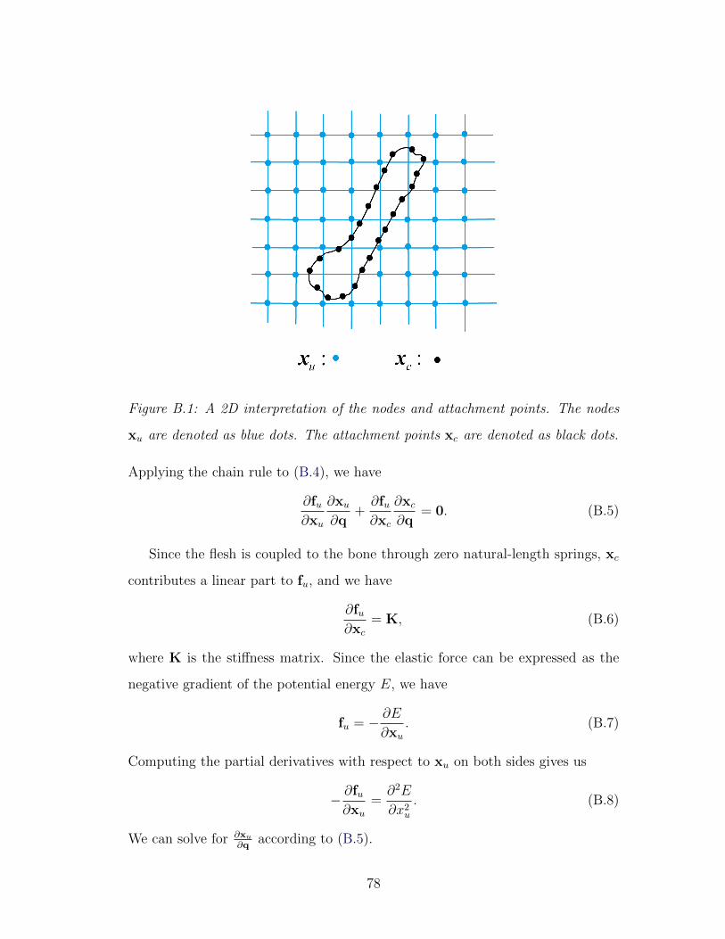
Figure B.1: A 2D interpretation of the nodes and attachment points. The nodes
xu are denoted as blue dots. The attachment points xc are denoted as black dots.
Applying the chain rule to (B.4), we have
∂fu∂xu
∂xu∂q
+∂fu∂xc
∂xc∂q
= 0. (B.5)
Since the flesh is coupled to the bone through zero natural-length springs, xc
contributes a linear part to fu, and we have
∂fu∂xc
= K, (B.6)
where K is the stiffness matrix. Since the elastic force can be expressed as the
negative gradient of the potential energy E, we have
fu = − ∂E∂xu
. (B.7)
Computing the partial derivatives with respect to xu on both sides gives us
− ∂fu∂xu
=∂2E
∂x2u
. (B.8)
We can solve for ∂xu
∂qaccording to (B.5).
78
Since the spring forces on the attachment points are fc = fc (xu,xc), we have
∂fc∂q
=∂fc∂xu
∂xu∂q
+∂fc∂xc
∂xc∂q
. (B.9)
Since both xu and xc contribute linearly to fc, we can easily compute ∂fc∂xu
and ∂fc∂xc
,
while ∂xc
∂qand ∂xu
∂qare already computed above, and we can compute ∂fc
∂qaccording
to (B.9).
79
APPENDIX C
Derivatives of B-splines
Given m real valued knots ti, with t0 ≤ t1 ≤ · · · ≤ tm−1, a B-spline of degree n is
a parametric curve
C : [tn, tm−n−1]→ R (C.1)
composed of a linear combination of basis B-splines Ni,n of degree n:
C(t) =m−n−2∑i=0
PiNi,n(t). (C.2)
The points Pi ∈ R are control points. The m− n− 1 basis B-splines of degree n
can be defined using the following recursion formula:
Nj,0(t) =
1, if tj ≤ t < tj+1, j = 0, ...,m− 2.
0, otherwise,
(C.3)
Nj,n(t) =t− tj
tj+n − tjNj,n−1(t) +
tj+n+1 − ttj+n+1 − tj+1
Nj+1,n−1(t), j = 0, ...,m− n− 2.
(C.4)
The first and second order derivatives of the basis B-splines can be computed
as follows:
d
dtNi,n(t) =
n
ti+n − tiNi,n−1(t)− n
ti+n−1 − tn+1
Ni+1,n−1(t); (C.5)
80
d2
dt2Ni,n(t) =
n
ti+n − tid
dtNi,n−1(t)− n
ti+n+1 − ti+1
d
dtNi+1,n−1(t)
=n
ti+n − ti
(n− 1
ti+n−1 − tiNi,n−2(t)− n− 1
ti+n − ti+1
Ni+1,n−2(t)
)− n
ti+n+1 − ti+1
(n− 1
ti+n − ti+1
Ni+1,n−2(t)− n− 1
ti+n+1 − ti+2
Ni+2,n−2(t)
)= n(n− 1)
(Ni,n−2(t)
(ti+n − ti)(ti++n−1 − ti)−(
1
(ti+n − ti)(ti+n − ti+1)
+1
(ti+n+1 − ti+1)(ti+n − ti+1)
)Ni+1,n−2(t) +
Ni+2,n−2(t)
(ti+n+1 − ti+1)(ti+n+1 − ti+2)
)(C.6)
So for the B-spline C(t), we can compute its first and second order derivatives
as follows:
dC(t)
dt=
m∑i=0
Pid
dtNi,n(t)
=m∑i=0
Pi
(n
ti+n − tiNi,n−1(t)− n
ti+n+1 − ti+1
Ni+1,n−1(t)
)= P0
n
tn − t0N0,n−1(t) +
∑i=1
m(Pi − Pi−1)n
tn+i − tiNi,n−1(t)
− Pmn
tm+n+1 − tm+1
Nm+1,n−1(t) (C.7)
d2C(t)
dt2=
m∑i=0
Pid2
dt2Ni,n(t)
= n(n− 1)
(N0,n−2(t)
P0
(tn − t0)(tn−1 − t0)
+N1,n−2(t)
(− P0
(tn − t0)(tn − t1)− fracP0 − P1(tn+1 − t1)(tn − t1)
)+
m∑i=2
Ni,n−2(t)
(Pi−2 − Pi−1
(ti+n−1 − ti−1)(ti+n−1 − ti)− Pi−1 − Pi
(ti+n − ti)(ti+n−1 − ti)
)+Nm+1,n−2(t)
(Pm−1 − Pm
(tm+n − tm)(tm+n − tm+1)− Pm
(tm+n+1 − tm+1)(tm+n − tm+1)
)+ Nm+2,n−2(t)
Pm(tm+n+1 − tm+1)(tm+n+1 − tm+2)
)(C.8)
81
APPENDIX D
Gaussian Process Dynamical Model Details
In order to characterize natural human motion, we train GPDMs using motion
capture data of a human swinging his arms and legs. Given the learned model
Γ = Y,X, α, β,W, the distribution over a new sequence Y and its associated
latent trajectory X is given by
p(Y, X|Γ
)= p
(Y|X,Γ
)p(X|Γ
). (D.1)
Here, Y ≡ [y1, · · · ,yN ]T are the observations (training data) and y1, · · · ,yN is a
sequence of observed feature vectors. In our application, we use joint angles as the
feature vector. X ≡ [x1, · · · ,xN ]T are the corresponding latent coordinates. Let
D be the dimension of the feature vector y, d the dimension of the latent vector
x, and W = diag (w1, · · · , wD) be a D ×D diagonal scaling matrix. We use two
previous frames to infer a new pose—i.e. we use the poses in frame n − 1 and
frame n to infer the new pose in frame n+1. Thus, we have Y = [yn−1, yn, yn+1]T ,
X = [xn−1, xn, xn+1]T . The distribution of p(Y|X,Γ
)is Gaussian and it can be
written as follows:
p(Y|X,Γ
)=
|W|M√(2π)MD |K(X)|D
exp
(−1
2tr(K−1(X)ZY W2ZT
Y
)), (D.2)
where M is the number of feature vectors in the new sequence; in our application
M = 3. We use the RBF kernel to define a kernel kY as
kY (x,x′) = exp
(−β1
2‖x− x′‖2
)+ β−1
2 δx,x′ , (D.3)
82
Now,
ZY = Y −KX,XK−1Y Y, (D.4)
and
K(X) = KX,X −KX,XK−1Y KT
X,X, (D.5)
where
KX,X =
kY (xn−1, xn−1) kY (xn−1, xn) kY (xn−1, xn+1)
kY (xn, xn−1) kY (xn, xn) kY (xn, xn+1)
kY (xn+1, xn−1) kY (xn+1, xn) kY (xn+1, xn+1)
(D.6)
and
KX,X =
kY (xn−1,x1) kY (xn−1,x2) · · · kY (xn−1,xN)
kY (xn,x1) kY (xn,x2) · · · kY (xn,xN)
kY (xn+1,x1) kY (xn+1,x2) · · · kY (xn+1,xN)
. (D.7)
The elements of the kernel matrix KY are defined by a kernel function (KY )ij ≡
kY (xi,xj). Matrix KY need only be inverted once by using the learned model.
The distribution p(X|Γ
)is not Gaussian, but it can be expressed similar to
(D.2):
p(X|Γ
)=
p (xn−1)√(2π)(M−1)d
exp
(−1
2tr(K−1(Xin)ZXZT
X
)). (D.8)
We use a “linear + RBF” kernel to define a kernel kX as follows:
kX(x,x′) = α1 exp(−α2
2‖x− x′‖2
)+ α3x
Tx′ + α−14 δx,x′ . (D.9)
Now,
ZX = Xout −KXin,XinK−1X Xout (D.10)
K(Xin
)= KXin,Xin
−KXin,XinK−1X K
TXin,Xin
. (D.11)
83
where
Xin = [x1, · · · ,xN−1]T , (D.12)
Xout = [x2, · · · ,xN ]T , (D.13)
Xin = [xn−1, xn]T , (D.14)
Xout = [xn, xn+1]T . (D.15)
The elements of the kernel matrix KX are defined by a kernel function (KX)ij ≡
kX (xi,xj) constructed from Xin, and KXin,Xin, and KXin,Xin
are defined similarly.
Matrix KX also needs only be inverted once by using the learned model.
Conditional Likelihood and Related Derivatives
The likelihood of a sequence with three feature vectors Y and the corresponding
latent positions X is computed as
LS(Y, X) = LY (Y, X) + LX(X), (D.16)
where
LY (Y, X) =D
2ln |K(X)|+ 1
2tr(K−1(X)ZY W2ZT
Y
)(D.17)
and
LX(X) =d
2ln |K(Xin)|+ 1
2tr(K−1(Xin)ZXZT
X
). (D.18)
Here, we also provide the partial derivatives of LS:
∂LS∂yn+1
=∂LY∂ZY
∂ZY
∂yn+1
, (D.19)
84
∂LS∂xn+1
=∂LY
∂K(X)
∂K(X)
∂xn+1
+∂LY∂ZY
∂ZY
∂xn+1
+∂LX∂ZX
∂ZX
∂xn+1
. (D.20)
In greater detail,
∂LY
∂K(X)=D
2K−1(X)− 1
2K−1(X)ZY W2ZT
Y K−1(X), (D.21)
∂LY∂ZY
= K−1(X)ZY W2, (D.22)
∂LX∂ZX
= K−1(Xin)ZX . (D.23)
Using xji to denote the j-th element of the latent vector xi,
∂K(X)
∂xjn+1
=∂KX,X
∂xjn+1
−∂(KX,XK−1
Y KTX,X
)∂xjn+1
. (D.24)
In greater detail,
∂KX,X
∂xjn+1
=
0 0 ∂kY (xn−1,xn+1)
∂xjn+1
0 0 ∂kY (xn,xn+1)
∂xjn+1
∂kY (xn+1,xn−1)
∂xjn+1
∂kY (xn+1,xn)
∂xjn+1
0
, (D.25)
where
∂kY (xi, xn+1)
∂xjn+1
=∂kY (xn+1, xi)
∂xjn+1
= −β1(xjn+1 − xji ) exp
(−β1
2‖xi − xn+1‖2
).
(D.26)
∂(KX,XK−1
Y KTX,X
)∂xjn+1
=N∑i=1
∂(KX,XK−1
Y KTX,X
)∂kY (xn+1,xi)
∂kY (xn+1,xi)
∂xjn+1
, (D.27)
where
∂(KX,XK−1
Y KTX,X
)∂kY (xn+1,xi)
= Gi + GTi (D.28)
85
and
Gi = E(3,i)3×NK−1
Y KTX,X
(D.29)
Here, we use E(3,i)3×N to denote a matrix whose elements are 0 except that the (3, i)
element is 1. Substituting (D.28) and (D.29) into (D.27), we have
∂(KX,XK−1
Y KTX,X
)∂xjn+1
= H + HT , (D.30)
where
H =
0 0 · · · 0
0 0 · · · 0
∂kY (xn+1,x1)
∂xjn+1
∂kY (xn+1,x2)
∂xjn+1
· · · ∂kY (xn+1,xN )
∂xjn+1
K−1Y KT
X,X. (D.31)
Furthermore,
∂ZY
∂xjn+1
= −
0 0 · · · 0
0 0 · · · 0
∂kY (xn+1,x1)
∂xjn+1
∂kY (xn+1,x2)
∂xjn+1
· · · ∂kY (xn+1,xN )
∂xjn+1
K−1Y Y, (D.32)
∂ZY
∂yjn+1
= E(3,j)3×D, (D.33)
and
∂ZX
∂xjn+1
= E(2,j)2×d . (D.34)
Partial Derivatives of the Naturalness Objective
To solve the nonlinear optimization problem (5.20) efficiently, we must provide
the partial derivative ∂Enat(xn+1)∂xn+1
. We apply chain rule to (5.20) and obtain
∂Enat (xn+1)
∂xn+1
=∂Eorient (q (µY (xn+1)))
∂q (µY (xn+1))
∂q (µY (xn+1))
∂µY (xn+1)
∂µY (xn+1)
∂xn+1
+ wprior∂LX(X)
∂xn+1
+ 2wsmooth (µY (xn+1)− µY (xn))T∂µY (xn+1)
∂xn+1
+ wconfid∂σ2
Y (xn+1)
∂xn+1
. (D.35)
86
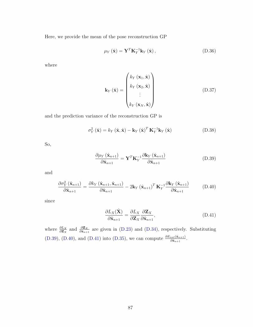
Here, we provide the mean of the pose reconstruction GP
µY (x) = YTK−1Y kY (x) , (D.36)
where
kY (x) =
kY (x1, x)
kY (x2, x)...
kY (xN , x)
(D.37)
and the prediction variance of the reconstruction GP is
σ2Y (x) = kY (x, x)− kY (x)T K−1
Y kY (x) (D.38)
So,
∂µY (xn+1)
∂xn+1
= YTK−1Y
∂kY (xn+1)
∂xn+1
(D.39)
and
∂σ2Y (xn+1)
∂xn+1
=∂kY (xn+1, xn+1)
∂xn+1
− 2kY (xn+1)T K−1Y
∂kY (xn+1)
∂xn+1
(D.40)
since
∂LX(X)
∂xn+1
=∂LX∂ZX
∂ZX
∂xn+1
, (D.41)
where ∂LX
∂ZXand ∂ZX
∂xn+1are given in (D.23) and (D.34), respectively. Substituting
(D.39), (D.40), and (D.41) into (D.35), we can compute ∂Enat(xn+1)∂xn+1
.
87
Bibliography
Agache, P., Monneur, C., Leveque, J., and Rigal, J. (1980). Mechanical properties
and Young’s modulus of human skin in vivo. Archives of Dermatological
Research, 269(3):221–232. 51
Albrecht, I., Haber, J., and Seidel, H.-P. (2003). Construction and animation of
anatomically based human hand models. In ACM SIGGRAPH/EG Symposium
on Computer Animation (SCA’03), pages 98–109. 8
Benson, D. J. (1992). Computational methods in Lagrangian and Eulerian
hydrocodes. Comput. Methods Appl. Mech. Eng., 99:235–394. 26
de Boor, C. (1978). A Practical Guide to Splines. Springer-Verlag. 34
Dong, F., Clapworthy, G. J., Krokos, M. A., and Yao, J. (2002). An anatomy-
based approach to human muscle modeling and deformation. IEEE Transac-
tions on Visualization and Computer Graphics, 8(2):154–170. 8
Enright, D., Marschner, S., and Fedkiw, R. (2002). Animation and rendering
of complex water surfaces. In Proceedings of the 29th Annual Conference on
Computer Graphics and Interactive Techniques, SIGGRAPH ’02, pages 736–
744, New York, NY. ACM. 24, 25
Faloutsos, P., van de Panne, M., and Terzopoulos, D. (2001). Composable
controllers for physics-based character animation. In Proceedings of the
28th Annual Conference on Computer Graphics and Interactive Techniques,
SIGGRAPH ’01, pages 251–260, New York, NY. ACM. 8
Featherstone, R. (1987). Robot Dynamics Algorithms. Kluwer Academic Publish-
ers, Boston. 16, 17
Fedkiw, R. P. (2002). Coupling an Eulerian fluid calculation to a Lagrangian solid
calculation with the ghost fluid method. J. Comput. Phys., 175:200–224. 26
88
Foster, N. and Fedkiw, R. (2001). Practical animation of liquids. In Proceedings of
the 28th Annual Conference on Computer Graphics and Interactive Techniques,
SIGGRAPH ’01, pages 23–30, New York, NY. ACM. 24, 25
Fung, Y. (1993). Biomechanics: Mechanical Properties of Living Tissues.
Springer, New York, NY. 16
Gams, A., Ijspeert, A. J., Schaal, S., and Lenarcic, J. (2009). On-line learning
and modulation of periodic movements with nonlinear dynamical systems.
Autonomous Robots, 27(1):3–23. 35, 37
Gill, P., Murray, W., and Saunders, M. (2002). SNOPT: An SQP algorithm
for large-scale constrained optimization. SIAM Journal on Optimization,
12(4):979–1006. 50
Grochow, K., Martin, S. L., Hertzmann, A., and Popovic, Z. (2004). Style-
based inverse kinematics. In Proceedings of the ACM SIGGRAPH Conference,
SIGGRAPH ’04, pages 522–531, New York, NY. ACM. 11
Grzeszczuk, R. and Terzopoulos, D. (1995). Automated learning of muscle-
actuated locomotion through control abstraction. In Proceedings of the ACM
SIGGRAPH Conference, Computer Graphics Proceedings, Annual Conference
Series, pages 63–70. 9, 11, 40
Hase, K., Miyashita, K., Ok, S., and Arakawa, Y. (2003). Human gait simulation
with a neuromusculoskeletal model and evolutionary computation. The Journal
of Visualization and Computer Animation, 14(2):73–92. 10
Ho, E. S. L., Komura, T., and Tai, C.-L. (2010). Spatial relationship preserving
character motion adaptation. In Proceedings of the ACM SIGGRAPH Confer-
ence, SIGGRAPH ’10, pages 33:1–33:8, New York, NY. ACM. 49
89
Hodgins, J. K., Wooten, W. L., Brogan, D. C., and O’Brien, J. F. (1995).
Animating human athletics. In Proceedings of the 22nd Annual Conference on
Computer Graphics and Interactive Techniques, SIGGRAPH ’95, pages 71–78,
New York, NY. ACM. 8
Ijspeert, A. J. (2008). Central pattern generators for locomotion control in animals
and robots: A review. Neural Networks, 21(4):642–653. 10
Ijspeert, A. J., Crespi, A., Ryczko, D., and Cabelguen, J.-M. (2007). From
swimming to walking with a salamander robot driven by a spinal cord model.
Science, 315(5817):1416–1420. 10
Ikemoto, L., Arikan, O., and Forsyth, D. (2009). Generalizing motion edits with
Gaussian processes. ACM Transactions on Graphics, 28(1):1:1–1:12. 11
Jacobson, A., Baran, I., Popovic, J., and Sorkine, O. (2011). Bounded biharmonic
weights for real-time deformation. ACM Transactions on Graphics (Proceedings
of the ACM SIGGRAPH Conference), 30(4):78:1–78:8. 67
Kavan, L., Collins, S., Zara, J., and O’Sullivan, C. (2008). Geometric skinning
with approximate dual quaternion blending. ACM Transactions on Graphics,
27(4):105. 67
Komura, T., Shinagawa, Y., and Kunii, T. L. (2000). Creating and retargetting
motion by the musculoskeletal human body model. The Visual Computer,
16(5):254–270. 8
Koren, Y. and Carmel, L. (2003). Visualization of labeled data using linear
transformations. In Proceedings of the Ninth Annual IEEE Conference on
Information Visualization, INFOVIS’03, pages 121–128, Washington, DC.
IEEE Computer Society. 75
90
Kwatra, N., Wojtan, C., Carlson, M., Essa, I., Mucha, P. J., and Turk, G. (2010).
Fluid simulation with articulated bodies. IEEE Transactions on Visualization
and Computer Graphics, 16:70–80. 9, 10
Lawrence, N. (2004). Gaussian process latent variable models for visualisation
of high dimensional data. Advances in Neural Information Processing Systems,
16:329–336. 11
Lee, S.-H., Sifakis, E., and Terzopoulos, D. (2009). Comprehensive biomechanical
modeling and simulation of the upper body. ACM Transactions on Graphics,
28:99:1–99:17. 8, 16, 19, 30, 40, 41, 42, 49, 67
Lee, S.-H. and Terzopoulos, D. (2006). Heads up! Biomechanical modeling and
neuromuscular control of the neck. In Proceedings of the ACM SIGGRAPH
Conference, SIGGRAPH ’06, pages 1188–1198, New York, NY. ACM. 8, 73
Lee, S.-H. and Terzopoulos, D. (2008). Spline joints for multibody dynamics.
ACM Transactions on Graphics, 27(3):22:1–22:8. 67
Lee, Y., Terzopoulos, D., and Waters, K. (1995). Realistic modeling for facial
animation. In Proceedings of ACM SIGGRAPH 95, Computer Graphics
Proceedings, Annual Conference Series, pages 55–62. 8
Lentine, M., Gretarsson, J. T., Schroeder, C., Robinson-Mosher, A., and Fedkiw,
R. (2011). Creature control in a fluid environment. IEEE Transactions on
Visualization and Computer Graphics, 17:682–693. 9, 11, 27
Levine, S., Wang, J. M., Haraux, A., Popovic, Z., and Koltun, V. (2012). Contin-
uous character control with low-dimensional embeddings. ACM Transactions
on Graphics, 31(4):28. 11, 47, 48
Ljung, L. and Soderstrom, T. (1983). Theory and Practice of Recursive Identifi-
cation. The MIT Press, Massachusetts and London. 37
91

MacKay-Lyons, M. (2002). Central pattern generation of locomotion: A review
of the evidence. Physical Therapy, 82(1):69–83. 10
McAdams, A., Zhu, Y., Selle, A., Empey, M., Tamstorf, R., Teran, J., and Sifakis,
E. (2011). Efficient elasticity for character skinning with contact and collisions.
In Proceedings of the ACM SIGGRAPH Conference, SIGGRAPH ’11, pages
37:1–37:12, New York, NY. ACM. 19, 30
Mukai, T. and Kuriyama, S. (2005). Geostatistical motion interpolation. In
Proceedings of the ACM SIGGRAPH Conference, SIGGRAPH ’05, pages 1062–
1070, New York, NY. ACM. 11
Nakamura, Y., Yamane, K., Fujita, Y., and Suzuki, I. (2005). Somatosensory
computation for man machine interface from motion-capture data and muscu-
loskeletal human model. IEEE Transactions on Robotics, 21(1):58–66. 8
Orin, D. and Goswami, A. (2008). Centroidal momentum matrix of a humanoid
robot: Structure and properties. In Proceedings of the IEEE/RSJ International
Conference on Intelligent Robots and Systems (IROS), pages 653 –659. 42
Patterson, T., Mitchell, N., and Sifakis, E. (2012). Simulation of complex
nonlinear elastic bodies using lattice deformers. ACM Transactions on Graphics,
31(6):197:1–197:10. 19, 22
Righetti, L. and Ijspeert, A. J. (2006). Programmable central pattern generators:
An application to biped locomotion control. In Proceedings of the 2006 IEEE
International Conference on Robotics and Automation, pages 1585–1590. 10
Schaal, S. and Atkeson, C. G. (1997). Constructive incremental learning from
only local information. Neural Computation, 10:2047–2084. 33
Sueda, S., Kaufman, A., and Pai, D. K. (2008). Musculotendon simulation for
hand animation. ACM Transactions on Graphics, 27(3):83:1–83:8. 8
92
Taga, G. (1995). A model of the neuro-musculo-skeletal system for human
locomotion. Biological Cybernetics, 73:113–121. 10
Tan, J., Gu, Y., Turk, G., and Liu, C. K. (2011). Articulated swimming creatures.
In Proceedings of the ACM SIGGRAPH Conference, SIGGRAPH ’11, pages
58:1–58:12, New York, NY. ACM. 9, 40
Thelen, D. G., Anderson, F. C., and Delp, S. L. (2003). Generating dynamic sim-
ulations of movement using computed muscle control. Journal of Biomechanics,
36(3):321–328. 40
Tsang, W., Singh, K., and Eugene, F. (2005). Helping hand: An anatomically
accurate inverse dynamics solution for unconstrained hand motion. In Proceed-
ings of the 2005 ACM SIGGRAPH/EG Symposium on Computer Animation,
SCA ’05, pages 319–328, New York, NY. ACM. 8
Tu, X. and Terzopoulos, D. (1994). Artificial fishes: Physics, locomotion, per-
ception, behavior. In Proceedings of the 21st Annual Conference on Computer
Graphics and Interactive Techniques, SIGGRAPH ’94, pages 43–50, New York,
NY. ACM. 9, 27, 68
Virtual-swim (2007). Aquatic Animation for Analysis and Education. http://
www.virtual-swim.com/. 34
Wang, J. M., Fleet, D. J., and Hertzmann, A. (2008). Gaussian process dynamical
models for human motion. IEEE Transactions on Pattern Analysis and Machine
Intelligence, 30(2):283–298. 47
Wang, J. M., Hamner, S. R., Delp, S. L., and Koltun, V. (2012). Optimizing
locomotion controllers using biologically-based actuators and objectives. ACM
Transactions on Graphics, 31(4):25:1–25:11. Proceedings of the ACM SIG-
GRAPH Conference. 8, 67
93
Waters, K. (1987). A muscle model for animating three-dimensional facial
expression. In Proceedings of the 14th Annual Conference on Computer Graphics
and Interactive Techniques, SIGGRAPH ’87, pages 17–24, New York, NY.
ACM. 8
Wei, X., Min, J., and Chai, J. (2011). Physically valid statistical models for human
motion generation. ACM Transactions on Graphics, 30(3):19:1–19:10. 11
Witkin, A. and Kass, M. (1988). Spacetime constraints. In Proceedings of the
15th Annual Conference on Computer Graphics and Interactive Techniques,
SIGGRAPH ’88, pages 159–168, New York, NY. ACM. 11
Yang, P.-F., Laszlo, J., and Singh, K. (2004). Layered dynamic control for inter-
active character swimming. In Proceedings of the 2004 ACM SIGGRAPH/EG
Symposium on Computer Animation, SCA ’04, pages 39–47, Aire-la-Ville,
Switzerland, Switzerland. Eurographics Association. 9, 10, 27
Ye, Y. and Liu, C. K. (2010). Synthesis of responsive motion using a dynamic
model. In Computer Graphics Forum (Proceedings of the Eurographics Confer-
ence). 11
Yu, J. and Turk, G. (2010). Reconstructing surfaces of particle-based fluids
using anisotropic kernels. In Proceedings of the 2010 ACM SIGGRAPH/EG
Symposium on Computer Animation, SCA ’10, pages 217–225, Aire-la-Ville,
Switzerland, Switzerland. Eurographics Association. 74
Zhu, Y., Sifakis, E., Teran, J., and Brandt, A. (2010). An efficient multigrid
method for the simulation of high-resolution elastic solids. ACM Transactions
on Graphics, 29(2):16:1–16:18. 19
Zordan, V. B., Celly, B., Chiu, B., and Dilorenzo, P. C. (2006). Breathe easy:
Model and control of human respiration for computer animation. Graphical
Models, 68:113–132. 8
94