realizing stock market crashes: stochastic cusp...

This article was downloaded by: [89.177.88.100]On: 29 September 2014, At: 13:00Publisher: RoutledgeInforma Ltd Registered in England and Wales Registered Number: 1072954 Registered office: MortimerHouse, 37-41 Mortimer Street, London W1T 3JH, UK

Quantitative FinancePublication details, including instructions for authors and subscription information:http://www.tandfonline.com/loi/rquf20

Realizing stock market crashes: stochastic cuspcatastrophe model of returns under time-varyingvolatilityJozef Barunikab & Jiri Kukackaab

a Institute of Economic Studies, Charles University, Opletalova 21, 110 00, Prague, CzechRepublic.b Institute of Information Theory and Automation, Academy of Sciences of the CzechRepublic, Pod Vodarenskou Vezi 4, 182 00, Prague, Czech Republic.Published online: 25 Sep 2014.

To cite this article: Jozef Barunik & Jiri Kukacka (2014): Realizing stock market crashes: stochastic cusp catastrophemodel of returns under time-varying volatility, Quantitative Finance, DOI: 10.1080/14697688.2014.950319

To link to this article: http://dx.doi.org/10.1080/14697688.2014.950319

PLEASE SCROLL DOWN FOR ARTICLE

Taylor & Francis makes every effort to ensure the accuracy of all the information (the “Content”) containedin the publications on our platform. However, Taylor & Francis, our agents, and our licensors make norepresentations or warranties whatsoever as to the accuracy, completeness, or suitability for any purpose ofthe Content. Any opinions and views expressed in this publication are the opinions and views of the authors,and are not the views of or endorsed by Taylor & Francis. The accuracy of the Content should not be reliedupon and should be independently verified with primary sources of information. Taylor and Francis shallnot be liable for any losses, actions, claims, proceedings, demands, costs, expenses, damages, and otherliabilities whatsoever or howsoever caused arising directly or indirectly in connection with, in relation to orarising out of the use of the Content.

This article may be used for research, teaching, and private study purposes. Any substantial or systematicreproduction, redistribution, reselling, loan, sub-licensing, systematic supply, or distribution in anyform to anyone is expressly forbidden. Terms & Conditions of access and use can be found at http://www.tandfonline.com/page/terms-and-conditions

http://www.tandfonline.com/loi/rquf20

http://www.tandfonline.com/action/showCitFormats?doi=10.1080/14697688.2014.950319

http://dx.doi.org/10.1080/14697688.2014.950319

http://www.tandfonline.com/page/terms-and-conditions

http://www.tandfonline.com/page/terms-and-conditions

Quantitative Finance, 2014http://dx.doi.org/10.1080/14697688.2014.950319

Realizing stock market crashes: stochastic cuspcatastrophe model of returns under time-varying

volatilityJOZEF BARUNIK∗†‡ and JIRI KUKACKA†‡

†Institute of Economic Studies, Charles University, Opletalova 21, 110 00 Prague, Czech Republic‡Institute of Information Theory and Automation, Academy of Sciences of the Czech Republic, Pod Vodarenskou Vezi 4,

182 00 Prague, Czech Republic

(Received 22 May 2013; accepted 25 July 2014)

This paper develops a two-step estimation methodology that allows us to apply catastrophe theoryto stock market returns with time-varying volatility and to model stock market crashes. In the firststep, we utilize high-frequency data to estimate daily realized volatility from returns. Then, we usestochastic cusp catastrophe theory on data normalized by the estimated volatility in the second stepto study possible discontinuities in the markets. We support our methodology through simulations inwhich we discuss the importance of stochastic noise and volatility in a deterministic cusp catastrophemodel. The methodology is empirically tested on nearly 27 years of US stock market returns coveringseveral important recessions and crisis periods. While we find that the stock markets showed signsof bifurcation in the first half of the period, catastrophe theory was not able to confirm this behaviourin the second half. Translating the results, we find that the US stock market’s downturns were morelikely to be driven by the endogenous market forces during the first half of the studied period, whileduring the second half of the period, exogenous forces seem to be driving the market’s instability.The results suggest that the proposed methodology provides an important shift in the application ofcatastrophe theory to stock markets.

Keywords: Stochastic cusp catastrophe model; Realized volatility; Bifurcations; Stock market crash

1. Introduction

Financial inefficiencies such as under- or over-reactions toinformation as the causes of extreme events in the stock mar-kets attract researchers across all fields of economics. In onerecent contribution, Levy (2008) highlighted the endogeneityof large market crashes as a result of the natural conformity ofinvestors with their peers in a heterogeneity inves-tor population. The stronger the conformity and homogeneityacross the market, the more likely the existence of multipleequilibria in the market, which is a prerequisite for a marketcrash to occur. Gennotte and Leland (1990) presented a modelthat shares the same notions as Levy (2008) in terms of theeffect of small changes when the market is close to a crash pointas well as the volatility amplification signalling. In anotherwork, Levy et al. (1994) considered the signals produced bydividend yields and assessed the effect of computer trading,which is blamed for making the market more homogeneous andthus more conducive to a crash. Kleidon (1995) summarized

∗Corresponding author. Email: [email protected]

and compared several older models from the 1980s and 1990s,and Barlevy and Veronesi (2003) proposed a model based onrational but uninformed traders who can unreasonably panic.Again with this approach, abrupt declines in stock prices canoccur without any real change in the underlying fundamentals.Lux (1995) linked the phenomena of market crashes to theprocess of phase transition from thermodynamics and mod-elled the emergence of bubbles and crashes as a result ofherd behaviour among heterogeneous traders in speculativemarkets. Finally, a strand of literature documenting precursorypatterns and log-periodic signatures years before the largestcrashes in the modern history suggested that crashes have anendogenous origin in ‘crowd’ behaviour and through the inter-actions of many agents (Sornette and Johansen 1998,Johansen et al. 2000, Sornette 2002, 2004). In contrast to manycommonly shared beliefs, Didier Sornette and his colleaguesargued that exogenous shocks can only serve as triggers andnot as the direct causes of crashes and that large crashes are‘outliers’.

Catastrophe theory provides a very different theoreticalframework to understand how even small shifts in the

© 2014 Taylor & Francis

Dow

nloa

ded

by [8

9.17

7.88

.100

] at 1

3:00

29

Sept

embe

r 201

4

2 J. Barunik and J. Kukacka

speculative part of the market can trigger a sudden, discon-tinuous effect on prices. Catastrophe theory was proposed byFrench mathematician Thom (1975) with the aim of shed-ding some light on the ‘mystery’ of biological morphogenesis.Despite its mathematical virtues, the theory was promptly heav-ily criticized by Zahler and Sussmann (1977) and Sussmannand Zahler (1978a,b) for its excessive utilization of qualitativeapproaches, the improper usage of certain statistical methodsand for violations of necessary mathematical assumptions inmany of its applications. Due to these criticisms, the intel-lectual bubble and the heyday of the cusp catastrophe app-roach declined rapidly after the 1970s, although the theorywas defended by some researchers, e.g. by Boutot (1993) andthe extensive, gradually updated work of Arnold (2004).Nonetheless, the ‘fatal’criticism was ridiculed by Rosser (2007,p. 3275 and 3257), who stated that the baby of catastrophetheory was largely thrown out with the bathwater of its inappro-priate applications, and the author suggested that economistsshould re-evaluate the former fad and move it to a more propervaluation.

The application of catastrophe theory in the social scienceshas not been as extensive as in the natural sciences, althoughit was utilized early in its existence. Zeeman’s (1974) coop-eration with Thom and his own popularization of the the-ory through the use of nontechnical examples (Zeeman 1975,Zeeman 1976) led to the development of many applicationsin the fields of economics, psychology, sociology, politicalstudies and others. Zeeman (1974) also proposed the applica-tion of the cusp catastrophe model to stock markets. Translat-ing seven qualitative hypotheses about stock exchanges to themathematical terminology of catastrophe theory produced oneof the first heterogeneous agent models for two main types ofinvestors: fundamentalists and chartists. Heterogeneity and theinteractions between these two distinct types of agents attractedwider attention in the behavioural finance literature. Funda-mentalists base their expectations about future asset prices ontheir beliefs about fundamental and economic factors such asdividends, earnings and the macroeconomic environment. Incontrast, chartists do not consider fundamentals in their tradingstrategies at all. Their expectations about future asset prices arebased on finding historical patterns in prices. While Zeeman’swork was only one qualitative description of observed bull andbear markets, it contained a number of important behaviouralelements that were later used in the large volume of literaturethat focused on heterogeneous agent modelling.† Today, thestatistical theory is well developed, and parameterized cuspcatastrophe models can be evaluated quantitatively based ondata.

The biggest difficulty in the application of catastrophe theoryarises from the fact that it stems from deterministic systems.Thus, it is difficult to apply it directly to systems that are subjectto random influences, which are common in the behaviouralsciences. Cobb and Watson (1980), Cobb (1981) and Cobb andZacks (1985) provided the necessary bridge and took catas-trophe theory from determinism to stochastic systems. Whilethis was an important shift, there are further complications

†For a recent survey of heterogeneous agent models, see Hommes(2006). A special issue on heterogeneous interacting agents infinancial markets edited by Lux and Marchesi (2002) also providesinteresting contributions.

in the theory’s application to stock market data. The mainrestriction of Cobb’s method of estimation was the requirementof a constant variance, which forces researchers to assume thatthe volatility of the stock markets (as the standard deviation ofthe returns) is constant. Quantitative verification of Zeeman’s(1974) hypotheses about the application of the theory to stockmarket crashes was pioneered by Barunik and Vosvrda (2009),where we fit the cusp model to two separate, large stock marketcrashes. However, the successful application of Barunik andVosvrda (2009) brought only preliminary results in a restrictedenvironment. Application of the cusp catastrophe theory onstock market data deserves much more attention. In the currentpaper, we propose an improved method of application thatwe believe brings us closer to an answer regarding whethercusp catastrophe theory is capable of explaining stock marketcrashes.

Time-varying volatility has become an important stylizedfact for stock market data, and researchers have recognized thatit is an important feature of any modelling strategy. One of themost successful early works of Engle (1982) and Bollerslev(1986) proposed including volatility as a time-varying pro-cess in a (generalized) autoregressive conditional heteroskeda-sticity framework. From that beginning, many models havebeen developed in the literature to improve the originalframeworks. As early as the late 1990s, high frequency databecame available to researchers, and this led to another impor-tant shift in volatility modelling — realized volatility. A verysimple, intuitive approach to compute daily volatility usingthe sum of squared high-frequency returns was formalized byAndersen et al. (2003) and Barndorff-Nielsen and Shephard(2004). While the volatility literature is immense,‡ severalresearchers have also studied volatility and stock marketcrashes. For example, Shaffer (1991) argued that volatilitymight be the cause of a stock market crash. In contrast, Levy(2008) argued that volatility increases before a crash, evenwhen no dramatic information is revealed.

In this study, we utilize the availability of high-frequencydata and the popular realized volatility approach to propose atwo-step method of estimation that overcomes the difficultiesin the application of cusp catastrophe theory to stock mar-ket data. Using realized volatility, we estimate stock marketreturns’ volatility, and then we apply the stochastic cusp catas-trophe model on volatility-adjusted returns with constant vari-ance. This approach is motivated by the confirmed bimodaldistributions of such standardized data in some periods, andit allows us to study whether stock markets are driven intocatastrophe endogenously or whether it is simply an effectof volatility. We run simulations that provide strong supportfor the methodology. The simulations also illustrate the im-portance of stochastic noise and volatility in the deterministiccusp model.

Using a unique data-set covering almost 27 years of theUS stock market evolution, we empirically test the stochasticcusp catastrophe model in a time-varying volatility environ-ment. Moreover, we develop a rolling regression approachto study the dynamics of the model’s parameters over a long

‡Andersen et al. (2004) provide a very useful and complete reviewof the methodologies.

Dow

nloa

ded

by [8

9.17

7.88

.100

] at 1

3:00

29

Sept

embe

r 201

4

Stochastic cusp catastrophe model of returns under time-varying volatility 3

period, covering several important recessions and crises. Thisapproach allows us to localize the bifurcation periods.

We need to mention several important works that providedsimilar results to ours. Creedy and Martin (1993) and Creedyet al. (1996) developed a framework for the estimation ofnon-linear exchange rate models, and they showed that swingsin exchange rates can be attributed to bimodality even withoutthe explicit use of catastrophe theory. More recently,Koh et al. (2007) proposed using Cardan’s discriminant todetect bimodality and confirmed the predictive ability of cur-rency pairs for emerging countries. In our work, we bring newinsight to the non-linear phenomena by including time-varyingvolatility in the modelling strategy.

The paper is organized as follows. The second and the thirdsections examine the theoretical framework of the stochasticcatastrophe theory under time-varying volatility and describethe model’s estimation. The fourth section presents the simu-lations that support our two-step method of estimation, and thefifth section presents the empirical application of the theory onthe modelling of stock market crashes. Finally, the last sectionconcludes.

2. Theoretical framework

Catastrophe theory was developed as a deterministic theoryfor systems that may respond to continuous changes in controlvariables by a discontinuous change from one equilibrium stateto another. A key idea is that the system under study is driventoward an equilibrium state. The behaviour of the dynamicalsystems under study is completely determined by a so-calledpotential function, which depends on behavioural and controlvariables. The behavioural, or state, variable describes the stateof the system, while control variables determine the behaviourof the system. The dynamics under catastrophe models canbecome extremely complex and according to the classifica-tion theory of Thom (1975), there are seven different familiesbased on the number of control and dependent variables. Wefocus on the application of catastrophe theory to model suddenstock market crashes, as qualitatively proposed by Zeeman(1974). In his work, Zeeman used the so-called cusp catastro-phe model, which is the simplest specification that gives riseto sudden discontinuities.

2.1. Deterministic dynamics

Let us suppose that the process yt evolves over t = 1, . . . , Tas

dyt = −dV (yt ;α,β)

dytdt, (1)

where V (yt ;α,β) is the potential function describing thedynamics of the state variable yt controlled by parametersα and β determining the system. When the right-hand side ofequation (1) equals zero, −dV (yt ;α,β)/dyt = 0, the systemis in equilibrium. If the system is at a state of non-equilibrium,it will move back to equilibrium where the potential functiontakes the minimum values with respect to yt . While the conceptof potential function is very general, i.e. it can be a quadraticfunction yielding equilibrium of a simple flat response surface,one of the most applied potential functions in behaviouralsciences, a cusp potential function, is defined as

−V (yt ;α,β) = −1/4y4t + 1/2βy2

t + αyt , (2)

with equilibria at

−dV (yt ;α,β)

dyt= −y3

t + βyt + α (3)

being equal to zero. The two dimensions of the control space,α and β, further depend on realizations from i = 1 . . . , n ofthe independent variables xi,t . Thus, it is convenient to thinkabout α and β as functions

αx = α0 + α1x1,t + . . . + αn xn,t (4)

βx = β0 + β1x1,t + . . . + βn xn,t . (5)

The control functions αx and βx are called normal and split-ting factors, or asymmetry and bifurcation factors, respectively(Stewart and Peregoy 1983), and they determine the predictedvalues of yt given xi,t . Therefore, for each combination ofvalues of independent variables, there could be up to threepredicted values of the state variable given by roots of

−dV (yt ;αx ,βx )

dyt= −y3

t + βx yt + αx = 0. (6)

This equation has one solution if

δx = 1/4α2x − 1/27β3

x (7)

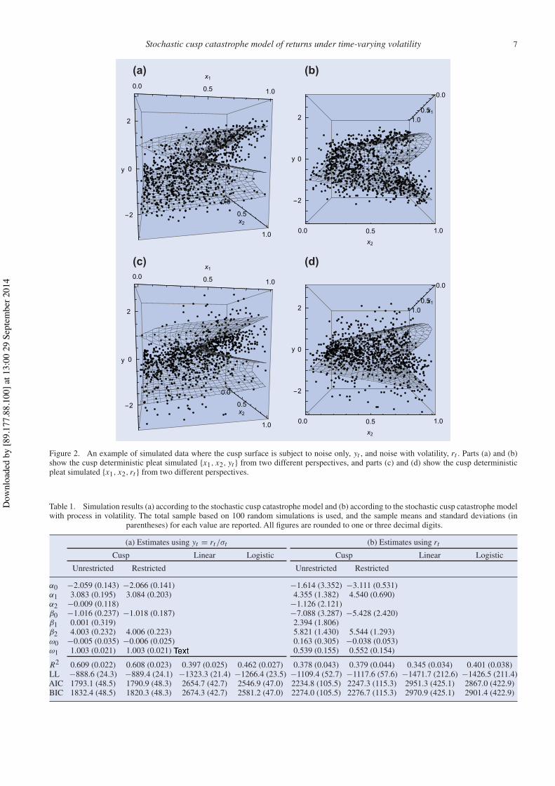
is greater than zero, δx > 0, and three solutions if δx < 0.This construction was first described by the sixteenth-centurymathematician Geronimo Cardan and can serve as a statisticfor bimodality, one of the catastrophe flags. The set of valuesfor which Cardan’s discriminant is equal to zero, δx = 0, is thebifurcation set that determines the set of singularity points inthe system. In the case of three roots, the central root is calledan ‘anti-prediction’and is the least probable state of the system.Inside the bifurcation, when δx < 0, the surface predicts twopossible values of the state variable, which means that in thiscase, the state variable is bimodal. For an illustration of thedeterministic response surface of cusp catastrophe, we borrowfrom figure 2 in the simulations section, where the deterministicresponse surface is a smooth pleat.

2.2. Stochastic dynamics

Most of the systems in behavioural sciences are subject to noisestemming from measurement errors or the inherent stochasticnature of the system under study. Thus, for real-world applica-tions, it is necessary to add non-deterministic behaviour into thesystem. Because catastrophe theory was primarily developedto describe deterministic systems, it may not be obvious howto extend the theory to stochastic systems. An important bridgewas provided by Cobb and Watson (1980), Cobb (1981) andCobb and Zacks (1985), who used the Itô stochastic differentialequations to establish a link between the potential function of adeterministic catastrophe system and the stationary probabilitydensity function of the corresponding stochastic process. Thisapproach in turn led to the definition of a stochastic equilibriumstate and bifurcation that was compatible with the deterministiccounterpart. Cobb and his colleagues simply added a stochasticGaussian white noise term to the system

dyt = −dV (yt ;αx ,βx )

dytdt + σyt dWt , (8)

Dow

nloa

ded

by [8

9.17

7.88

.100

] at 1

3:00

29

Sept

embe

r 201

4


where −dV (yt ;αx ,βx )/dyt is the deterministic term, or driftfunction representing the equilibrium state of the cusp catastro-phe, σyt is the diffusion function and Wt is a Wiener process.When the diffusion function is constant, σyt = σ , and thecurrent measurement scale is not to be nonlinearly transformed,the stochastic potential function is proportional to the determin-istic potential function, and the probability distribution func-tion corresponding to the solution from equation (8) convergesto a probability distribution function of a limiting stationarystochastic process because the dynamics of yt are assumedto be much faster than changes in xi,t (Cobb 1981, Cobb andZacks 1985, Wagenmakers et al. 2005). The probability densitythat describes the distribution of the system’s states at any t isthen

fs(y|x) = ψ exp!

(−1/4)y4 + (βx/2)y2 + αx yσ

". (9)

The constant ψ normalizes the probability distribution func-tion, so its integral over the entire range equals one. As thebifurcation factor βx changes from negative to positive, thefs(y|x) changes its shape from unimodal to bimodal. Con-versely, αx causes asymmetry in fs(y|x).

2.3. Cusp catastrophe under time-varying volatility

Stochastic catastrophe theory works only under the assumptionthat the diffusion function is constant, σyt = σ , and the cur-rent measurement scale is not to be nonlinearly transformed.While this assumption may be reliable in some applicationsin the behavioural sciences, it may cause crucial difficultiesin others. One of the problematic applications is in modellingstock market crashes because the diffusion function σ , calledthe volatility of stock market returns, has strong time-varyingdynamics, and it clusters over time, which is documented bystrong dependence in the squared returns. To illustrate thevolatility dynamics, let us borrow the data-set used later inthis study. Figure 4 shows the evolution of the S&P 500 stockindex returns over almost 27 years and documents how volatil-ity strongly varies over time. One of the possible and verysimple solutions in applying cusp catastrophe theory to thestock markets is to consider only a short-time window andto fit the catastrophe model to data where volatility can be as-sumed to be constant (Barunik and Vosvrda 2009). Although inBarunik and Vosvrda (2009) we were the first to quantitativelyapply stochastic catastrophes to explain stock market crasheson localized periods of crashes, this assumption is generallyvery restrictive.

Here, we propose a more rigorous solution to the problemby utilizing the recently developed concept of realized volatil-ity. This approach allows us to use the previously introducedconcepts after estimating the volatility from the returns processconsistently, and we are able to estimate the catastrophe modelon the process that fulfils the assumptions of the stochasticcatastrophe theory. Thus, we assume that stock markets canbe described by the cusp catastrophe process subject to time-varying volatility. While this approach represents a great ad-vantage that allows us to apply cusp catastrophe theory todifferent time periods conveniently, the disadvantage is thatthe method cannot be generalized to other branches of the be-havioural sciences where high-frequency data are not available

and therefore realized volatility cannot be computed. Thus, ourgeneralization is mainly restricted to applications on financialdata. Still, our main aim is to study stock market crashes, andtherefore the advocated approach is very useful in the field ofbehavioural finance. We now describe the theoretical concept,and in the next sections, we will present the full model and thetwo-step estimation procedure.

Suppose that the sample path of the corresponding (latent)logarithmic price process pt is continuous over t = 1, . . . , Tand determined by the stochastic differential equation

d pt = µt dt + σt dWt , (10)

where µt is a drift term, σt is the predictable diffusion functionor instantaneous volatility, and Wt is a standard Brownianmotion.Anatural measure of the ex-post return variability overthe [t − h, t] time interval, 0 ≤ h ≤ t ≤ T is the integratedvariance

I Vt,h =# t

t−hσ 2τ dτ, (11)

which is not directly observed, but as shown by Andersenet al. (2003) and Barndorff-Nielsen and Shephard (2004), thecorresponding realized volatilities provide its consistent esti-mates. While it is convenient to work in the continuous timeenvironment, empirical investigations are based on discretelysampled prices, and we are interested in studying h-period con-tinuously compounded discrete-time returns rt,h = pt − pt−h .Andersen et al. (2003) and Barndorff-Nielsen and Shephard(2004) showed that daily returns are Gaussian, conditional onan information set generated by the sample paths of µt and σt ,and integrated volatility normalizes the returns as

rt,h

!# t

t−hσ 2τ dτ

"−1/2

∼ N!# t

t−hµτdτ, 1

". (12)

This result of quadratic variation theory is important to usbecause we use it to study stochastic cusp catastrophe in anenvironment where volatility is time varying. In the modernstochastic volatility literature, it is common to assume thatstock market returns follow the very general semi-martingaleprocess (as in equation 10), where the drift and volatility func-tions are predictable and the rest is unpredictable. In the originsof this stream of literature, one of the very first contributionspublished regarding stochastic volatility by Taylor (1982) as-sumed that daily returns are the product of a volatility andautoregression process. In our application, we also assume thatdaily stock market returns are described by a process that is theproduct of volatility and the cusp catastrophe model.

To formulate the approach, we assume that stock returnsnormalized by their volatility

y∗t = rt

!# t

t−hσ 2τ dτ

"−1/2

(13)

follow a stochastic cusp catastrophe process

dy∗t = −dV (y∗

t ;αx ,βx )

dy∗t

dt + dWt . (14)

It is important to note the difference between equation (14) andequation (8) because there is no longer any diffusion term inthe process. Because the diffusion term of y∗

t is constant andnow equal to one, Cobb’s results can conveniently be used, andwe can use the stationary probability distribution function of

Dow

nloa

ded

by [8

9.17

7.88

.100

] at 1

3:00

29

Sept

embe

r 201

4


y∗t for the parameter estimation using the maximum likelihood

method.As noted previously, the integrated volatility is not directly

observable. However, the now-popular concept of realizedvolatility and the availability of high-frequency data providea simple method to accurately measure integrated volatility,which helps us propose a simple and intuitive method to esti-mate the cusp catastrophe model on stock market returns underhighly dynamic volatility.

3. Estimation

A simple, consistent estimator of the integrated variance underthe assumption of no microstructure noise contamination in theprice process is provided by the well-known realized variance(Andersen et al. 2003, Barndorff-Nielsen and Shephard 2004).The realized variance over [t − h, t], for 0 ≤ h ≤ t ≤ T , isdefined by

$RV t,h =N%

i=1

r2t−h+

&iN

'h, (15)

where N is the number of observations in [t − h, t], andr

t−h+&

iN

'h

is i−th intraday return in the [t − h, t] interval.

$RV t converges in probability to the true integrated variance ofthe process as N → ∞.

$RV t,hp→

# t

t−hσ 2τ dτ, (16)

As observed, the log-prices are contaminated with micro-structure noise in the real world, and the literature has deve-loped several estimators. While it is important to considerboth jumps and microstructure noise in the data, our maininterest is in estimating the catastrophe theory and addressingthe question whether it can be used to explain the deterministicportion of stock market returns. Thus, we restrict ourselves tothe simplest estimator, which uses sparse sampling to deal withthe microstructure noise. The extant literature showed supportfor this simple estimator; most recently, Liu et al. (2012) ran ahorse race for the most popular estimators and concluded thatwhen simple realized volatility is computed using five-minutesampling, it is very difficult to outperform.

In the first step, we estimate realized volatility from thestock market returns using five-minute data as proposed bythe theory, and we normalize the daily returns to obtain returnswith constant volatility. While using the daily returns, h = 1,and we henceforth drop h for ease of notation.

r̃t = rt $RV −1/2t (17)

In the second step, we apply the stochastic cusp catastropheto model the normalized stock market returns. While the statevariable of the cusp is a canonical variable, it is an unknownsmooth transformation of the actual state variable of the sys-tem. As proposed by Grasman et al. (2009), we allow forthe first-order approximation to the true, smooth transitionallowing the measured r̃ to be a

yt = ω0 + ω1r̃t , (18)

with ω1 as the first-order coefficient of a polynomial approxi-mation. The independent variables are

αx = α0 + α1x1,t + . . . + αn xn,t (19)

βx = β0 + β1x1,t + . . . + βn xn,t , (20)

Hence, the statistical estimation problem is to estimate 2n + 2parameters {ω0,ω1,α0, . . . ,αn,β0, . . . , . . . ,βn}. We estimatethe parameters using the maximum likelihood approach ofCobb and Watson (1980) as augmented by Grasman et al.(2009). The negative log-likelihood for a sample of observedvalues (x1,t , . . . , xn,t , yt ) for t = 1, . . . , T is simply the loga-rithm of the probability distribution function in equation (9).

3.1. Statistical evaluation of the fit

To assess the fit of the cusp catastrophe model to the data, anumber of diagnostic tools have been suggested. Stewart andPeregoy (1983) proposed a pseudo-R2 as a measure of theexplained variance. However, a difficulty arises here becausefor a given set of values of the independent variables, themodel may predict multiple values for the dependent variable.Because of bimodal density, the expected value is unlikely tobe observed because it is an unstable solution at equilibrium.For this reason, two alternatives for the expected value asthe predictive value can be used. The first method choosesthe mode of the density closest to the state values, which isknown as the delay convention; the second method uses themode at which the density is highest, which is known as theMaxwell convention. Cobb and Watson (1980) and Stewart andPeregoy (1983) suggested using the delay convention wherethe variance of the error is defined as the variance of the dif-ference between the estimated states and then using the modeof the distribution that is closest to this value. The pseudo-R2

is defined as 1 − V ar(ϵ)/V ar(y), where ϵ is error.While pseudo-R2 is problematic due to the nature of the

cusp catastrophe model, it should be used in a complementaryfashion to other alternatives. To rigorously test the statisticalfit of the cusp catastrophe model, we use following steps.First, the cusp fit should be substantially better than multiplelinear regression. The cusp fit could be tested by means ofa likelihood ratio test, which is asymptotically chi-squareddistributed with degrees of freedom equal to the difference indegrees of freedom for two compared models. Second, the ω1coefficient should deviate significantly from zero. Otherwise,the yt in equation (18) would be constant, and the cusp modelwould not describe the data. Third, the cusp model should showa better fit than the following logistic curve:

yt = 1

1 + e−αt /β2t

+ ϵt , (21)

for t = 1, . . . , T , where ϵt are zero-mean random disturbances.The rationale for choosing to compare the cusp model to thislogistic curve is that this function does not possess degeneratepoints, while it possibly models steep changes in the statevariable as a function of changes in the independent variablesmimicking the sudden transitions of the cusp. Thus, a com-parison of the cusp catastrophe model to the logistic functionserves as a good indicator of the presence of bifurcations in thedata. While these two models are not nested, Wagenmakerset al. (2005) suggested comparing them via information

Dow

nloa

ded

by [8

9.17

7.88

.100

] at 1

3:00

29

Sept

embe

r 201

4


(a) (b) (c) (d)

Figure 1. An example of a simulated time series where the cusp surface is subject to noise only, yt , and noise together with volatility, rt . (b)simulated returns yt (a) kernel density estimate of yt (c) simulated returns rt contaminated with volatility (d) kernel density estimate of rt .

criteria, where a stronger Bayesian Information Criterion (BIC)should be required for the decision.

4. Monte Carlo study

To validate our assumptions about the process of generatingstock market returns and our two-step estimation procedure,we conduct a Monte Carlo study where we simulate the datafrom the stochastic cusp catastrophe model, allow for time-varying volatility in the process and estimate the parameters tosee whether we can recover the true values.

We simulate the data from the stochastic cusp catastrophemodel subject to time-varying volatility as

rt = σt yt (22)

dσ 2t = κ(ω − σ 2

t )dt + γ dWt,1, (23)

dyt = (αt + βt yt − y3t )dt + dWt,2 (24)

where dWt,1 and dWt,2 are standard Brownian motions withzero correlation, κ = 5, ω = 0.04 and γ = 0.5. The volatilityparameters satisfy Feller’s condition 2κω ≥ γ 2, which keepsthe volatility process away from the zero boundary. We set theparameters to values that are reasonable for a stock price, as inZhang et al. (2005).

In the cusp equation, we use two independent variables

αt = α0 + α1xt,1 + α2xt,2 (25)

βt = β0 + β1xt,1 + β2xt,2 (26)

with coefficients α2 = β1 = 0. Hence xt,1 drawn from theU (0, 1) distribution drives the asymmetry side, and xt,2 drawnfrom the U (0, 1) distribution drives the bifurcation side of themodel. The parameters are set as α0 = −2, α1 = 3, β0 = −1and β2 = 4.

In the simulations, we are interested in determining how thecusp catastrophe model performs under time-varying volatility.Thus, we estimate the coefficients on the processes yt = rt/σtand rt . Figure 1 shows one realization of the simulated returnsyt and rt . While yt is the cusp catastrophe subject to noise, rt issubject to time-varying volatility as well. It is noticeable howtime-varying volatility causes the shift from bimodal densityto unimodal. More illustrative is figure 2, which shows thecusp catastrophe surface of both processes. While the solutionfrom the deterministic cusp catastrophe is contaminated withnoise in the first case, the volatility process in the second casemakes it much more difficult to recognize the two states of the

system in the bifurcation area. This result causes difficulty inrecovering the true parameters.

Table 1 shows the results of the simulation. We simulatethe processes 100 times and report the mean and standarddeviations from the mean.† The true parameters are easilyrecovered in the simulations from yt when the cusp catastropheis subject to noise only because the mean values are statisticallyindistinguishable from the true simulated values α0 = −2,α1 = 3, β0 = −1 and β2 = 4. The fits are reasonablebecause they explain approximately 60% of the data variationin the noisy environment. Moreover, in the cusp model, we firstestimate the full set of parameters (α0,α1,α2,β0,β1,β2), andthen we restrict the parameters α2 = β1 = 0. The estimationeasily recovers the true parameters in both cases, while in theunrestricted case, the estimates α2 = β1 = 0 and fits are sta-tistically the same. In comparison, both cusp models performmuch better than logistic regression and linear models, whichwas expected. It is also interesting to note that ω0 = 0 andω1 = 1, which means that the observed data are the true data,and no transformation is needed. These results are importantbecause they confirm that the estimation of the stochastic cuspcatastrophe model is valid, and it can be used to quantitativelyapply the theory to the data.

The results of the estimation on the rt process, which issubject to time-varying volatility, reveal that the addition of thevolatility process makes it difficult for the maximum likelihoodestimation to recover the true parameters. The variances of theestimated parameters are very large, and the means are faraway from the true simulated values. Moreover, the fits arestatistically weaker, as they explain no more than 38% of thevariance in the data. It is also interesting to note that the logisticfit and the linear fit are much closer to the cusp fit.

In conclusion, the simulation results reveal that time-varyingvolatility in the cusp catastrophe model destroys the ability ofthe maximum likelihood estimator to recover the cusp poten-tial.

5. Empirical modelling of stock market crashes

Armed with the results from the simulations, we move to theestimation of the cusp catastrophe model on the real-world data

†The distribution of the parameters is Gaussian in both cases, whichmakes it possible to compare the results within the means and standarddeviations.

Dow

nloa

ded

by [8

9.17

7.88

.100

] at 1

3:00

29

Sept

embe

r 201

4


(a)

(c)

(b)

(d)

Figure 2. An example of simulated data where the cusp surface is subject to noise only, yt , and noise with volatility, rt . Parts (a) and (b)show the cusp deterministic pleat simulated {x1, x2, yt } from two different perspectives, and parts (c) and (d) show the cusp deterministicpleat simulated {x1, x2, rt } from two different perspectives.

Table 1. Simulation results (a) according to the stochastic cusp catastrophe model and (b) according to the stochastic cusp catastrophe modelwith process in volatility. The total sample based on 100 random simulations is used, and the sample means and standard deviations (in

parentheses) for each value are reported. All figures are rounded to one or three decimal digits.

(a) Estimates using yt = rt/σt (b) Estimates using rt

Cusp Linear Logistic Cusp Linear Logistic

Unrestricted Restricted Unrestricted Restricted

α0 −2.059 (0.143) −2.066 (0.141) −1.614 (3.352) −3.111 (0.531)α1 3.083 (0.195) 3.084 (0.203) 4.355 (1.382) 4.540 (0.690)α2 −0.009 (0.118) −1.126 (2.121)β0 −1.016 (0.237) −1.018 (0.187) −7.088 (3.287) −5.428 (2.420)β1 0.001 (0.319) 2.394 (1.806)β2 4.003 (0.232) 4.006 (0.223) 5.821 (1.430) 5.544 (1.293)ω0 −0.005 (0.035) −0.006 (0.025) 0.163 (0.305) −0.038 (0.053)ω1 1.003 (0.021) 1.003 (0.021) 0.539 (0.155) 0.552 (0.154)

R2 0.609 (0.022) 0.608 (0.023) 0.397 (0.025) 0.462 (0.027) 0.378 (0.043) 0.379 (0.044) 0.345 (0.034) 0.401 (0.038)LL −888.6 (24.3) −889.4 (24.1) −1323.3 (21.4) −1266.4 (23.5) −1109.4 (52.7) −1117.6 (57.6) −1471.7 (212.6) −1426.5 (211.4)AIC 1793.1 (48.5) 1790.9 (48.3) 2654.7 (42.7) 2546.9 (47.0) 2234.8 (105.5) 2247.3 (115.3) 2951.3 (425.1) 2867.0 (422.9)BIC 1832.4 (48.5) 1820.3 (48.3) 2674.3 (42.7) 2581.2 (47.0) 2274.0 (105.5) 2276.7 (115.3) 2970.9 (425.1) 2901.4 (422.9)

Dow

nloa

ded

by [8

9.17

7.88

.100

] at 1

3:00

29

Sept

embe

r 201

4

Barunik

Text


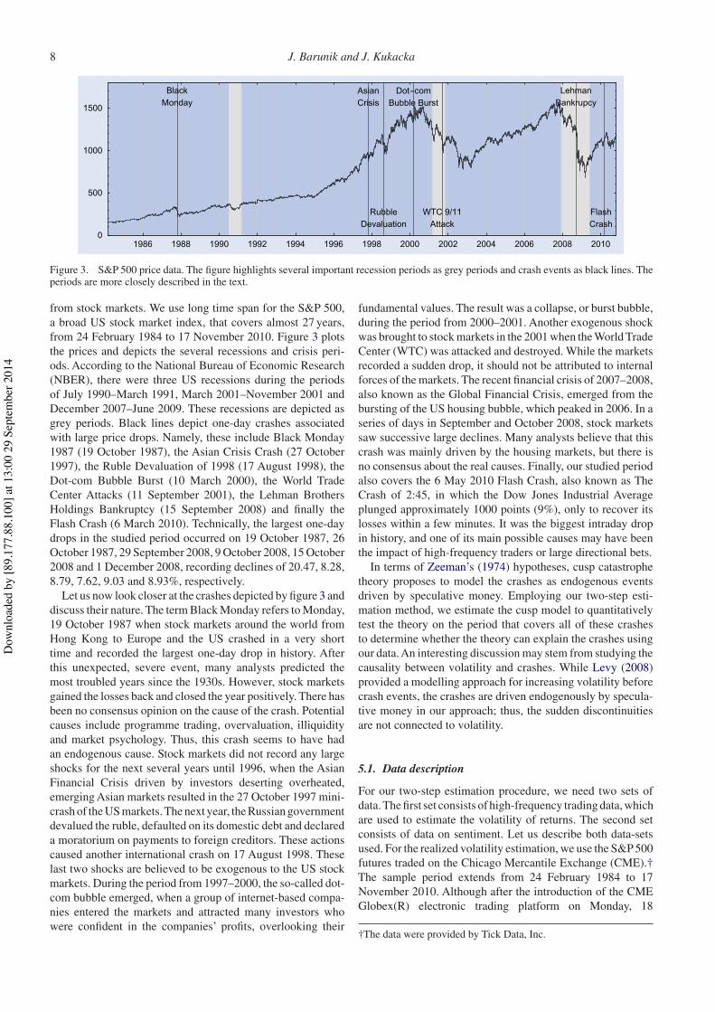
Figure 3. S&P 500 price data. The figure highlights several important recession periods as grey periods and crash events as black lines. Theperiods are more closely described in the text.

from stock markets. We use long time span for the S&P 500,a broad US stock market index, that covers almost 27 years,from 24 February 1984 to 17 November 2010. Figure 3 plotsthe prices and depicts the several recessions and crisis peri-ods. According to the National Bureau of Economic Research(NBER), there were three US recessions during the periodsof July 1990–March 1991, March 2001–November 2001 andDecember 2007–June 2009. These recessions are depicted asgrey periods. Black lines depict one-day crashes associatedwith large price drops. Namely, these include Black Monday1987 (19 October 1987), the Asian Crisis Crash (27 October1997), the Ruble Devaluation of 1998 (17 August 1998), theDot-com Bubble Burst (10 March 2000), the World TradeCenter Attacks (11 September 2001), the Lehman BrothersHoldings Bankruptcy (15 September 2008) and finally theFlash Crash (6 March 2010). Technically, the largest one-daydrops in the studied period occurred on 19 October 1987, 26October 1987, 29 September 2008, 9 October 2008, 15 October2008 and 1 December 2008, recording declines of 20.47, 8.28,8.79, 7.62, 9.03 and 8.93%, respectively.

Let us now look closer at the crashes depicted by figure 3 anddiscuss their nature. The term Black Monday refers to Monday,19 October 1987 when stock markets around the world fromHong Kong to Europe and the US crashed in a very shorttime and recorded the largest one-day drop in history. Afterthis unexpected, severe event, many analysts predicted themost troubled years since the 1930s. However, stock marketsgained the losses back and closed the year positively. There hasbeen no consensus opinion on the cause of the crash. Potentialcauses include programme trading, overvaluation, illiquidityand market psychology. Thus, this crash seems to have hadan endogenous cause. Stock markets did not record any largeshocks for the next several years until 1996, when the AsianFinancial Crisis driven by investors deserting overheated,emerging Asian markets resulted in the 27 October 1997 mini-crash of the US markets.The next year, the Russian governmentdevalued the ruble, defaulted on its domestic debt and declareda moratorium on payments to foreign creditors. These actionscaused another international crash on 17 August 1998. Theselast two shocks are believed to be exogenous to the US stockmarkets. During the period from 1997–2000, the so-called dot-com bubble emerged, when a group of internet-based compa-nies entered the markets and attracted many investors whowere confident in the companies’ profits, overlooking their

fundamental values. The result was a collapse, or burst bubble,during the period from 2000–2001. Another exogenous shockwas brought to stock markets in the 2001 when the World TradeCenter (WTC) was attacked and destroyed. While the marketsrecorded a sudden drop, it should not be attributed to internalforces of the markets. The recent financial crisis of 2007–2008,also known as the Global Financial Crisis, emerged from thebursting of the US housing bubble, which peaked in 2006. In aseries of days in September and October 2008, stock marketssaw successive large declines. Many analysts believe that thiscrash was mainly driven by the housing markets, but there isno consensus about the real causes. Finally, our studied periodalso covers the 6 May 2010 Flash Crash, also known as TheCrash of 2:45, in which the Dow Jones Industrial Averageplunged approximately 1000 points (9%), only to recover itslosses within a few minutes. It was the biggest intraday dropin history, and one of its main possible causes may have beenthe impact of high-frequency traders or large directional bets.

In terms of Zeeman’s (1974) hypotheses, cusp catastrophetheory proposes to model the crashes as endogenous eventsdriven by speculative money. Employing our two-step esti-mation method, we estimate the cusp model to quantitativelytest the theory on the period that covers all of these crashesto determine whether the theory can explain the crashes usingour data.An interesting discussion may stem from studying thecausality between volatility and crashes. While Levy (2008)provided a modelling approach for increasing volatility beforecrash events, the crashes are driven endogenously by specula-tive money in our approach; thus, the sudden discontinuitiesare not connected to volatility.

5.1. Data description

For our two-step estimation procedure, we need two sets ofdata.The first set consists of high-frequency trading data, whichare used to estimate the volatility of returns. The second setconsists of data on sentiment. Let us describe both data-setsused. For the realized volatility estimation, we use the S&P 500futures traded on the Chicago Mercantile Exchange (CME).†The sample period extends from 24 February 1984 to 17November 2010. Although after the introduction of the CMEGlobex(R) electronic trading platform on Monday, 18

†The data were provided by Tick Data, Inc.

Dow

nloa

ded

by [8

9.17

7.88

.100

] at 1

3:00

29

Sept

embe

r 201

4


(a)

(b)

(c)

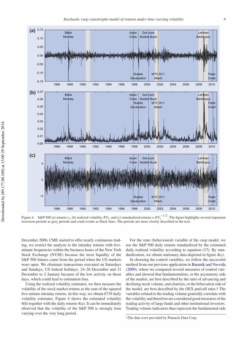
Figure 4. S&P 500 (a) returns rt , (b) realized volatility RVt , and (c) standardized returns rt RV −1/2t . The figure highlights several important

recession periods as grey periods and crash events as black lines. The periods are more closely described in the text.

December 2006, CME started to offer nearly continuous trad-ing, we restrict the analysis to the intraday returns with five-minute frequencies within the business hours of the New YorkStock Exchange (NYSE) because the most liquidity of theS&P 500 futures came from the period when the US marketswere open. We eliminate transactions executed on Saturdaysand Sundays, US federal holidays, 24–26 December and 31December to 2 January because of the low activity on thosedays, which could lead to estimation bias.

Using the realized volatility estimator, we then measure thevolatility of the stock market returns as the sum of the squaredfive-minute intraday returns. In this way, we obtain 6739 dailyvolatility estimates. Figure 4 shows the estimated volatility4(b) together with the daily returns 4(a). It can be immediatelyobserved that the volatility of the S&P 500 is strongly timevarying over the very long period.

For the state (behavioural) variable of the cusp model, weuse the S&P 500 daily returns standardized by the estimateddaily realized volatility according to equation (17). By stan-dardization, we obtain stationary data depicted in figure 4(c).

In choosing the control variables, we follow the successfulmethod from our previous application in Barunik and Vosvrda(2009), where we compared several measures of control vari-ables and showed that fundamentalists, or the asymmetry sideof the market, are best described by the ratio of advancing anddeclining stock volume, and chartists, or the bifurcation side ofthe model, are best described by the OEX put/call ratio.† Thevariables related to the trading volume generally correlate withthe volatility and therefore are considered good measures of thetrading activity of large funds and other institutional investors.Trading volume indicators thus represent the fundamental side

†The data were provided by Pinnacle Data Corp.

Dow

nloa

ded

by [8

9.17

7.88

.100

] at 1

3:00

29

Sept

embe

r 201

4


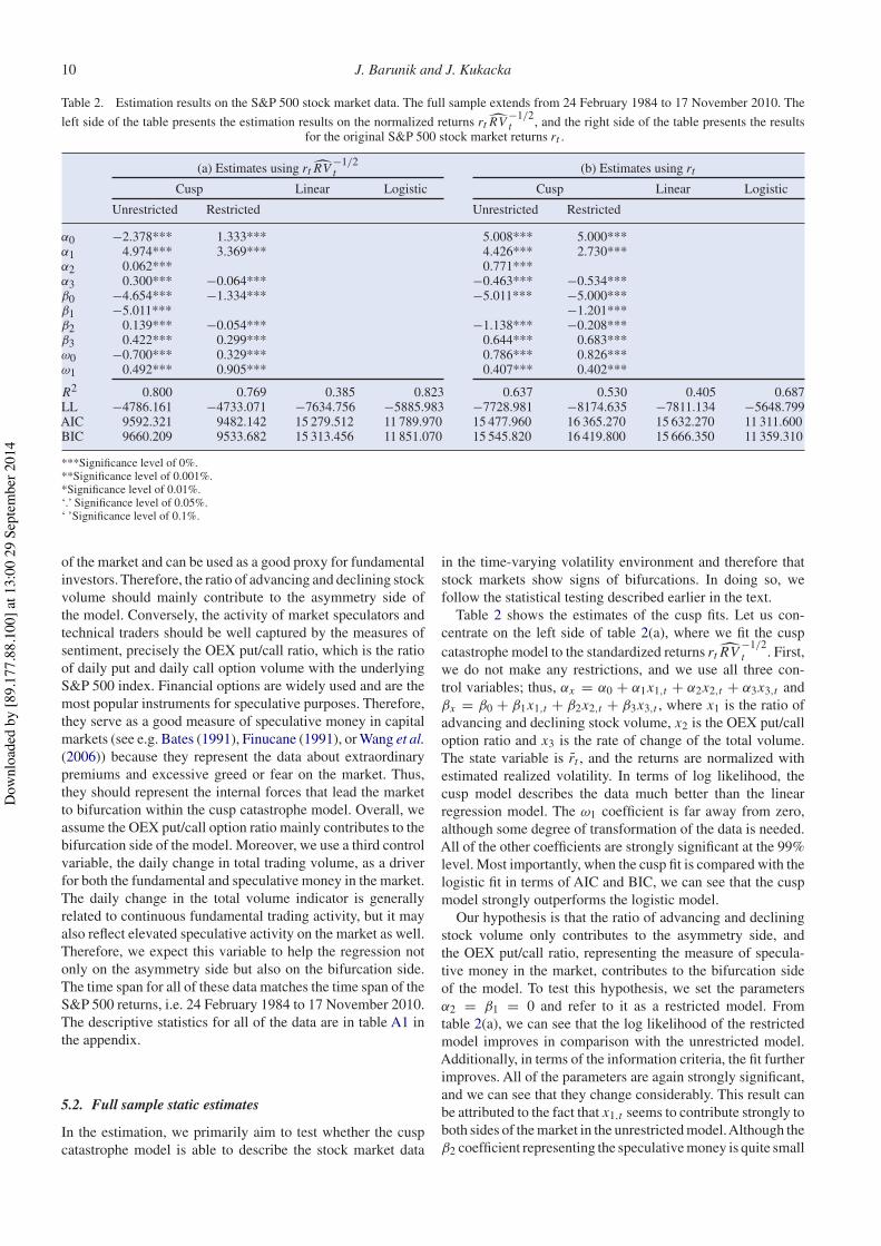
Table 2. Estimation results on the S&P 500 stock market data. The full sample extends from 24 February 1984 to 17 November 2010. Theleft side of the table presents the estimation results on the normalized returns rt $RV −1/2

t , and the right side of the table presents the resultsfor the original S&P 500 stock market returns rt .

(a) Estimates using rt $RV −1/2t (b) Estimates using rt



α0 −2.378*** 1.333*** 5.008*** 5.000***α1 4.974*** 3.369*** 4.426*** 2.730***α2 0.062*** 0.771***α3 0.300*** −0.064*** −0.463*** −0.534***β0 −4.654*** −1.334*** −5.011*** −5.000***β1 −5.011*** −1.201***β2 0.139*** −0.054*** −1.138*** −0.208***β3 0.422*** 0.299*** 0.644*** 0.683***ω0 −0.700*** 0.329*** 0.786*** 0.826***ω1 0.492*** 0.905*** 0.407*** 0.402***

R2 0.800 0.769 0.385 0.823 0.637 0.530 0.405 0.687LL −4786.161 −4733.071 −7634.756 −5885.983 −7728.981 −8174.635 −7811.134 −5648.799AIC 9592.321 9482.142 15 279.512 11 789.970 15 477.960 16 365.270 15 632.270 11 311.600BIC 9660.209 9533.682 15 313.456 11 851.070 15 545.820 16 419.800 15 666.350 11 359.310

***Significance level of 0%.**Significance level of 0.001%.*Significance level of 0.01%.‘.’ Significance level of 0.05%.‘ ’Significance level of 0.1%.

of the market and can be used as a good proxy for fundamentalinvestors. Therefore, the ratio of advancing and declining stockvolume should mainly contribute to the asymmetry side ofthe model. Conversely, the activity of market speculators andtechnical traders should be well captured by the measures ofsentiment, precisely the OEX put/call ratio, which is the ratioof daily put and daily call option volume with the underlyingS&P 500 index. Financial options are widely used and are themost popular instruments for speculative purposes. Therefore,they serve as a good measure of speculative money in capitalmarkets (see e.g. Bates (1991), Finucane (1991), or Wang et al.(2006)) because they represent the data about extraordinarypremiums and excessive greed or fear on the market. Thus,they should represent the internal forces that lead the marketto bifurcation within the cusp catastrophe model. Overall, weassume the OEX put/call option ratio mainly contributes to thebifurcation side of the model. Moreover, we use a third controlvariable, the daily change in total trading volume, as a driverfor both the fundamental and speculative money in the market.The daily change in the total volume indicator is generallyrelated to continuous fundamental trading activity, but it mayalso reflect elevated speculative activity on the market as well.Therefore, we expect this variable to help the regression notonly on the asymmetry side but also on the bifurcation side.The time span for all of these data matches the time span of theS&P 500 returns, i.e. 24 February 1984 to 17 November 2010.The descriptive statistics for all of the data are in table A1 inthe appendix.

5.2. Full sample static estimates

In the estimation, we primarily aim to test whether the cuspcatastrophe model is able to describe the stock market data

in the time-varying volatility environment and therefore thatstock markets show signs of bifurcations. In doing so, wefollow the statistical testing described earlier in the text.

Table 2 shows the estimates of the cusp fits. Let us con-centrate on the left side of table 2(a), where we fit the cuspcatastrophe model to the standardized returns rt $RV −1/2

t . First,we do not make any restrictions, and we use all three con-trol variables; thus, αx = α0 + α1x1,t + α2x2,t + α3x3,t andβx = β0 + β1x1,t + β2x2,t + β3x3,t , where x1 is the ratio ofadvancing and declining stock volume, x2 is the OEX put/calloption ratio and x3 is the rate of change of the total volume.The state variable is r̃t , and the returns are normalized withestimated realized volatility. In terms of log likelihood, thecusp model describes the data much better than the linearregression model. The ω1 coefficient is far away from zero,although some degree of transformation of the data is needed.All of the other coefficients are strongly significant at the 99%level. Most importantly, when the cusp fit is compared with thelogistic fit in terms of AIC and BIC, we can see that the cuspmodel strongly outperforms the logistic model.

Our hypothesis is that the ratio of advancing and decliningstock volume only contributes to the asymmetry side, andthe OEX put/call ratio, representing the measure of specula-tive money in the market, contributes to the bifurcation sideof the model. To test this hypothesis, we set the parametersα2 = β1 = 0 and refer to it as a restricted model. Fromtable 2(a), we can see that the log likelihood of the restrictedmodel improves in comparison with the unrestricted model.Additionally, in terms of the information criteria, the fit furtherimproves. All of the parameters are again strongly significant,and we can see that they change considerably. This result canbe attributed to the fact that x1,t seems to contribute strongly toboth sides of the market in the unrestricted model.Although theβ2 coefficient representing the speculative money is quite small

Dow

nloa

ded

by [8

9.17

7.88

.100

] at 1

3:00

29

Sept

embe

r 201

4


in comparison with the other coefficients, it is still stronglysignificant. Because this coefficient is the key for the model indriving the stock market to bifurcation, we further investigateits impact in the following sections. It is interesting to note thatthe ω1 parameter increases very close to one in the restrictedmodel. This result means that the observed data are close tothe state variable.

When moving to the right (b) side of table 2, we repeat thesame analysis, but this time, we use the original rt returns asthe state variable. We wish to compare the cusp catastrophe fitto the data with strongly varying volatility. In using the data’svery long time span where the volatility varies considerably,we expect the model to deteriorate. Although the applicationof the cusp catastrophe model to the non-stationary data can bequestioned, we provide these estimates to compare them withour modelling approach. We see an important result. While thelinear and logistic models provide very similar fits in terms ofthe log likelihoods, the information criteria and R2 deterioratein both the unrestricted and restricted cusp models. The ω1coefficient, together with all of the other coefficients, is stillstrongly different from zero, but the important result is thatthe logistic model not only describes the data better, but alsothe presence of bifurcations in the raw return data cannot beclaimed.

To conclude this section, the results suggest strong evidencethat over the long period of almost 27 years, the stock marketsare better described by the cusp catastrophe model. Using ourtwo-step modelling approach, we have shown that the cuspmodel fits the data well and the fundamental and bifurcationsides are controlled by the indicators for the fundamental andspeculative money, respectively. In contrast, when the cusp isfit to the original data with a strong variation in volatility, themodel deteriorates. We should note that these results resem-ble the results from the simulation; thus, the simulation alsostrongly supports our modelling approach.

5.3. Examples of the 1987 and 2008 crashes

While the results from the previous section are supportive of thecusp catastrophe model, the sample period of almost 27 yearsmay contain many structural changes. Thus, we wish to fur-ther investigate how the model performs over time. Therefore,we use the two very distinct crashes of 1987 and 2008 andcompare them to the localized cusp fits. There are severalreasons to study these particular periods. These crashes weredistinct in time, as there were 21 years between them, so theyoffer us an opportunity to determine how the data describethe periods. On the one hand, the stock market crash of 1987has not yet been explained, and many analysts believe it wasan endogenous crash. Therefore, it constitutes a perfect candi-date for the cusp model. On the other hand, the 2008 periodcovered a much deeper recession, so it was very different from1987. Finally, the two periods contain all of the largest one-daydrops, which occurred on 19 October 1987, 26 October 1987,29 September 2008, 9 October 2008, 15 October 2008 and1 December 2008, recording declines of 20.47, 8.28, 8.79, 7.62,9.03 and 8.93%, respectively. In the following estimations, werestrict ourselves to our newly proposed two-step approach for

the cusp catastrophe fitting procedure, and we utilize samplescovering one-half year.

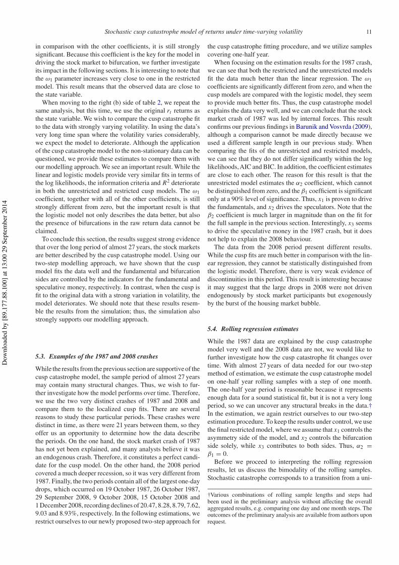
When focusing on the estimation results for the 1987 crash,we can see that both the restricted and the unrestricted modelsfit the data much better than the linear regression. The ω1coefficients are significantly different from zero, and when thecusp models are compared with the logistic model, they seemto provide much better fits. Thus, the cusp catastrophe modelexplains the data very well, and we can conclude that the stockmarket crash of 1987 was led by internal forces. This resultconfirms our previous findings in Barunik and Vosvrda (2009),although a comparison cannot be made directly because weused a different sample length in our previous study. Whencomparing the fits of the unrestricted and restricted models,we can see that they do not differ significantly within the loglikelihoods,AIC and BIC. In addition, the coefficient estimatesare close to each other. The reason for this result is that theunrestricted model estimates the α2 coefficient, which cannotbe distinguished from zero, and the β1 coefficient is significantonly at a 90% level of significance. Thus, x1 is proven to drivethe fundamentals, and x2 drives the speculators. Note that theβ2 coefficient is much larger in magnitude than on the fit forthe full sample in the previous section. Interestingly, x3 seemsto drive the speculative money in the 1987 crash, but it doesnot help to explain the 2008 behaviour.

The data from the 2008 period present different results.While the cusp fits are much better in comparison with the lin-ear regression, they cannot be statistically distinguished fromthe logistic model. Therefore, there is very weak evidence ofdiscontinuities in this period. This result is interesting becauseit may suggest that the large drops in 2008 were not drivenendogenously by stock market participants but exogenouslyby the burst of the housing market bubble.

5.4. Rolling regression estimates

While the 1987 data are explained by the cusp catastrophemodel very well and the 2008 data are not, we would like tofurther investigate how the cusp catastrophe fit changes overtime. With almost 27 years of data needed for our two-stepmethod of estimation, we estimate the cusp catastrophe modelon one-half year rolling samples with a step of one month.The one-half year period is reasonable because it representsenough data for a sound statistical fit, but it is not a very longperiod, so we can uncover any structural breaks in the data.†In the estimation, we again restrict ourselves to our two-stepestimation procedure. To keep the results under control, we usethe final restricted model, where we assume that x1 controls theasymmetry side of the model, and x2 controls the bifurcationside solely, while x3 contributes to both sides. Thus, α2 =β1 = 0.

Before we proceed to interpreting the rolling regressionresults, let us discuss the bimodality of the rolling samples.Stochastic catastrophe corresponds to a transition from a uni-

†Various combinations of rolling sample lengths and steps hadbeen used in the preliminary analysis without affecting the overallaggregated results, e.g. comparing one day and one month steps. Theoutcomes of the preliminary analysis are available from authors uponrequest.

Dow

nloa

ded

by [8

9.17

7.88

.100

] at 1

3:00

29

Sept

embe

r 201

4


Table 3. Estimation results for the two distinct periods of the S&P 500 normalized stock market returns, rt $RV −1/2t .

1987 2008



α0 −0.970* −0.535*** −3.938*** −0.598***α1 1.792*** 1.794*** 1.793*** 1.798***α2 −0.073 −1.322α3 0.191 0.029 −0.814 0.005***β0 0.562* 0.322* −0.542*** −1.142*β1 −0.395* −1.803***β2 −1.255** −0.731* −0.990** −0.031***β3 1.648*** 1.547*** −0.803 0.282ω0 0.453*** 0.771*** −0.637*** 0.680***ω1 0.561*** 0.602*** 0.476*** 0.641***

R2 0.855 0.827 0.454 0.895 0.816 0.858 0.483 0.884LL −85.971 −90.659 −208.557 −104.045 −88.054 −103.437 −185.150 −90.148AIC 191.943 197.317 427.114 226.089 196.108 222.875 380.300 198.296BIC 220.385 220.071 441.335 251.687 224.550 245.628 394.521 223.894

***Significance level of 0%.**Significance level of 0.001%.*Significance level of 0.01%.‘.’Significance level of 0.05%.‘ ’Significance level of 0.1%.

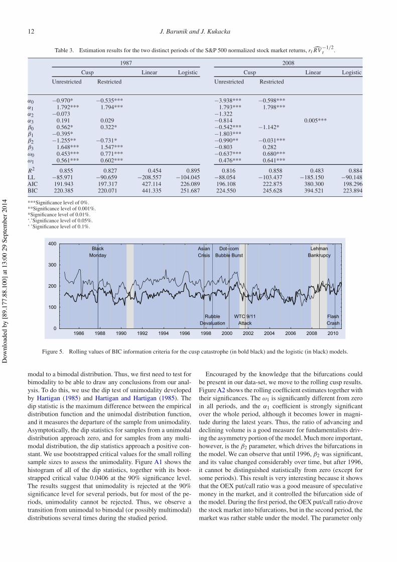
Figure 5. Rolling values of BIC information criteria for the cusp catastrophe (in bold black) and the logistic (in black) models.

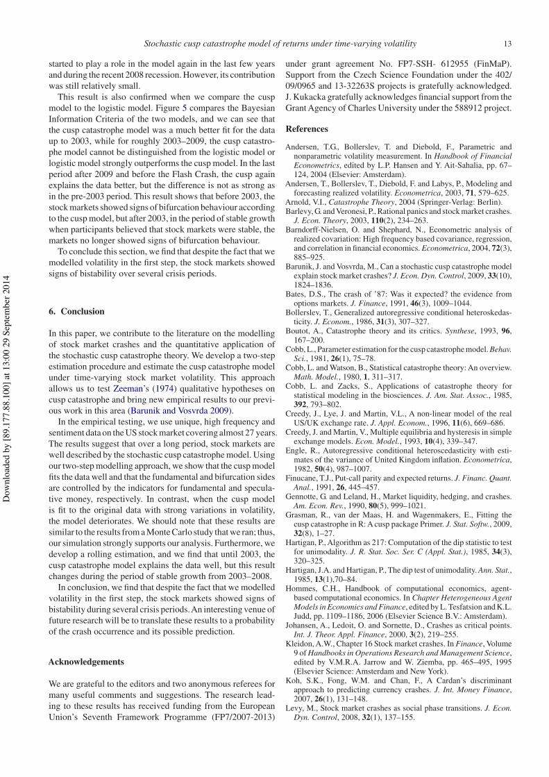
modal to a bimodal distribution. Thus, we first need to test forbimodality to be able to draw any conclusions from our anal-ysis. To do this, we use the dip test of unimodality developedby Hartigan (1985) and Hartigan and Hartigan (1985). Thedip statistic is the maximum difference between the empiricaldistribution function and the unimodal distribution function,and it measures the departure of the sample from unimodality.Asymptotically, the dip statistics for samples from a unimodaldistribution approach zero, and for samples from any multi-modal distribution, the dip statistics approach a positive con-stant. We use bootstrapped critical values for the small rollingsample sizes to assess the unimodality. Figure A1 shows thehistogram of all of the dip statistics, together with its boot-strapped critical value 0.0406 at the 90% significance level.The results suggest that unimodality is rejected at the 90%significance level for several periods, but for most of the pe-riods, unimodality cannot be rejected. Thus, we observe atransition from unimodal to bimodal (or possibly multimodal)distributions several times during the studied period.

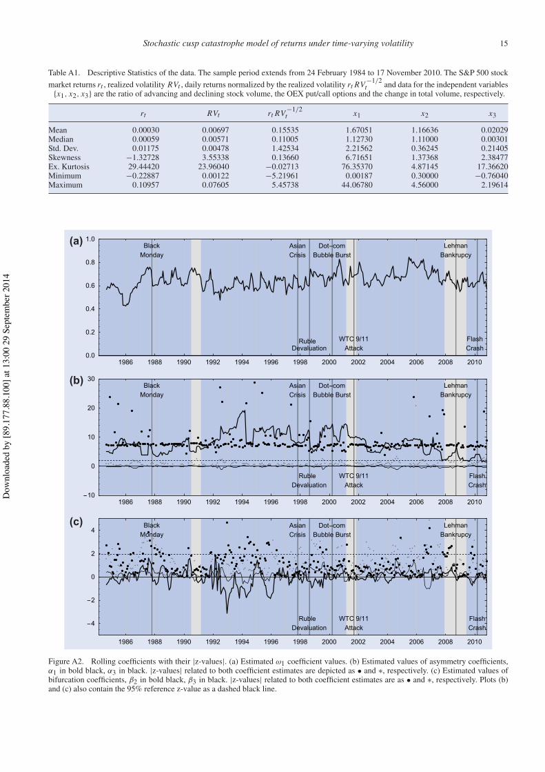
Encouraged by the knowledge that the bifurcations couldbe present in our data-set, we move to the rolling cusp results.Figure A2 shows the rolling coefficient estimates together withtheir significances. The ω1 is significantly different from zeroin all periods, and the α1 coefficient is strongly significantover the whole period, although it becomes lower in magni-tude during the latest years. Thus, the ratio of advancing anddeclining volume is a good measure for fundamentalists driv-ing the asymmetry portion of the model. Much more important,however, is the β2 parameter, which drives the bifurcations inthe model. We can observe that until 1996, β2 was significant,and its value changed considerably over time, but after 1996,it cannot be distinguished statistically from zero (except forsome periods). This result is very interesting because it showsthat the OEX put/call ratio was a good measure of speculativemoney in the market, and it controlled the bifurcation side ofthe model. During the first period, the OEX put/call ratio drovethe stock market into bifurcations, but in the second period, themarket was rather stable under the model. The parameter only

Dow

nloa

ded

by [8

9.17

7.88

.100

] at 1

3:00

29

Sept

embe

r 201

4


started to play a role in the model again in the last few yearsand during the recent 2008 recession. However, its contributionwas still relatively small.

This result is also confirmed when we compare the cuspmodel to the logistic model. Figure 5 compares the BayesianInformation Criteria of the two models, and we can see thatthe cusp catastrophe model was a much better fit for the dataup to 2003, while for roughly 2003–2009, the cusp catastro-phe model cannot be distinguished from the logistic model orlogistic model strongly outperforms the cusp model. In the lastperiod after 2009 and before the Flash Crash, the cusp againexplains the data better, but the difference is not as strong asin the pre-2003 period. This result shows that before 2003, thestock markets showed signs of bifurcation behaviour accordingto the cusp model, but after 2003, in the period of stable growthwhen participants believed that stock markets were stable, themarkets no longer showed signs of bifurcation behaviour.

To conclude this section, we find that despite the fact that wemodelled volatility in the first step, the stock markets showedsigns of bistability over several crisis periods.

6. Conclusion

In this paper, we contribute to the literature on the modellingof stock market crashes and the quantitative application ofthe stochastic cusp catastrophe theory. We develop a two-stepestimation procedure and estimate the cusp catastrophe modelunder time-varying stock market volatility. This approachallows us to test Zeeman’s (1974) qualitative hypotheses oncusp catastrophe and bring new empirical results to our previ-ous work in this area (Barunik and Vosvrda 2009).

In the empirical testing, we use unique, high frequency andsentiment data on the US stock market covering almost 27 years.The results suggest that over a long period, stock markets arewell described by the stochastic cusp catastrophe model. Usingour two-step modelling approach, we show that the cusp modelfits the data well and that the fundamental and bifurcation sidesare controlled by the indicators for fundamental and specula-tive money, respectively. In contrast, when the cusp modelis fit to the original data with strong variations in volatility,the model deteriorates. We should note that these results aresimilar to the results from a Monte Carlo study that we ran; thus,our simulation strongly supports our analysis. Furthermore, wedevelop a rolling estimation, and we find that until 2003, thecusp catastrophe model explains the data well, but this resultchanges during the period of stable growth from 2003–2008.

In conclusion, we find that despite the fact that we modelledvolatility in the first step, the stock markets showed signs ofbistability during several crisis periods.An interesting venue offuture research will be to translate these results to a probabilityof the crash occurrence and its possible prediction.

Acknowledgements

We are grateful to the editors and two anonymous referees formany useful comments and suggestions. The research lead-ing to these results has received funding from the EuropeanUnion’s Seventh Framework Programme (FP7/2007-2013)

under grant agreement No. FP7-SSH- 612955 (FinMaP).Support from the Czech Science Foundation under the 402/09/0965 and 13-32263S projects is gratefully acknowledged.J. Kukacka gratefully acknowledges financial support from theGrant Agency of Charles University under the 588912 project.

References

Andersen, T.G., Bollerslev, T. and Diebold, F., Parametric andnonparametric volatility measurement. In Handbook of FinancialEconometrics, edited by L.P. Hansen and Y. Ait-Sahalia, pp. 67–124, 2004 (Elsevier: Amsterdam).

Andersen, T., Bollerslev, T., Diebold, F. and Labys, P., Modeling andforecasting realized volatility. Econometrica, 2003, 71, 579–625.

Arnold, V.I., Catastrophe Theory, 2004 (Springer-Verlag: Berlin).Barlevy, G. and Veronesi, P., Rational panics and stock market crashes.

J. Econ. Theory, 2003, 110(2), 234–263.Barndorff-Nielsen, O. and Shephard, N., Econometric analysis of

realized covariation: High frequency based covariance, regression,and correlation in financial economics. Econometrica, 2004, 72(3),885–925.

Barunik, J. and Vosvrda, M., Can a stochastic cusp catastrophe modelexplain stock market crashes? J. Econ. Dyn. Control, 2009, 33(10),1824–1836.

Bates, D.S., The crash of ’87: Was it expected? the evidence fromoptions markets. J. Finance, 1991, 46(3), 1009–1044.

Bollerslev, T., Generalized autoregressive conditional heteroskedas-ticity. J. Econom., 1986, 31(3), 307–327.

Boutot, A., Catastrophe theory and its critics. Synthese, 1993, 96,167–200.

Cobb, L., Parameter estimation for the cusp catastrophe model. Behav.Sci., 1981, 26(1), 75–78.

Cobb, L. and Watson, B., Statistical catastrophe theory: An overview.Math. Model., 1980, 1, 311–317.

Cobb, L. and Zacks, S., Applications of catastrophe theory forstatistical modeling in the biosciences. J. Am. Stat. Assoc., 1985,392, 793–802.

Creedy, J., Lye, J. and Martin, V.L., A non-linear model of the realUS/UK exchange rate. J. Appl. Econom., 1996, 11(6), 669–686.

Creedy, J. and Martin, V., Multiple equilibria and hysteresis in simpleexchange models. Econ. Model., 1993, 10(4), 339–347.

Engle, R., Autoregressive conditional heteroscedasticity with esti-mates of the variance of United Kingdom inflation. Econometrica,1982, 50(4), 987–1007.

Finucane, T.J., Put-call parity and expected returns. J. Financ. Quant.Anal., 1991, 26, 445–457.

Gennotte, G. and Leland, H., Market liquidity, hedging, and crashes.Am. Econ. Rev., 1990, 80(5), 999–1021.

Grasman, R., van der Maas, H. and Wagenmakers, E., Fitting thecusp catastrophe in R: A cusp package Primer. J. Stat. Softw., 2009,32(8), 1–27.

Hartigan, P., Algorithm as 217: Computation of the dip statistic to testfor unimodality. J. R. Stat. Soc. Ser. C (Appl. Stat.), 1985, 34(3),320–325.

Hartigan, J.A. and Hartigan, P., The dip test of unimodality. Ann. Stat.,1985, 13(1),70–84.

Hommes, C.H., Handbook of computational economics, agent-based computational economics. In Chapter Heterogeneous AgentModels in Economics and Finance, edited by L. Tesfatsion and K.L.Judd, pp. 1109–1186, 2006 (Elsevier Science B.V.: Amsterdam).

Johansen, A., Ledoit, O. and Sornette, D., Crashes as critical points.Int. J. Theor. Appl. Finance, 2000, 3(2), 219–255.

Kleidon, A.W., Chapter 16 Stock market crashes. In Finance, Volume9 of Handbooks in Operations Research and Management Science,edited by V.M.R.A. Jarrow and W. Ziemba, pp. 465–495, 1995(Elsevier Science: Amsterdam and New York).

Koh, S.K., Fong, W.M. and Chan, F., A Cardan’s discriminantapproach to predicting currency crashes. J. Int. Money Finance,2007, 26(1), 131–148.

Levy, M., Stock market crashes as social phase transitions. J. Econ.Dyn. Control, 2008, 32(1), 137–155.

Dow

nloa

ded

by [8

9.17

7.88

.100

] at 1

3:00

29

Sept

embe

r 201

4


Levy, M., Levy, H. and Solomon, S.,Amicroscopic model of the stockmarket: Cycles, booms, and crashes. Econ. Lett., 1994, 45(1), 103–111.

Liu, L., Patton,A. and Sheppard, K., Does anything beat 5-minute RV?A comparison of realized measures across multiple asset classes.Working Paper, Duke University and University of Oxford, 2012.

Lux, T., Herd behaviour, bubles and crashes. Econ. J., 1995, 105,881–896.

Lux, T. and Marchesi, M., Journal of economic behavior andorganization: Special issue on heterogeneous interacting agents infinancial markets. J. Econ. Behav. Organiz., 2002, 49(2), 143–147.

Rosser, J.B.J., The rise and fall of catastrophe theory applications ineconomics: Was the baby thrown out with the bathwater? J. Econ.Dyn. Control, 2007, 31, 3255–3280.

Shaffer, S., Structural shifts and the volatility of chaotic markets. J.Econ. Behav. Organiz., 1991, 15(2), 201–214.

Sornette, D., Predictability of catastrophic events: Material rupture,earthquakes, turbulence, financial crashes, and human birth. Proc.Nat. Acad. Sci. U.S.A., 2002, 99, 2522–2529.

Sornette, D., Why Stock Markets Crash: Critical Events in ComplexFinancial Systems, 2004 (Princeton University Press: Princeton,NJ).

Sornette, D. and Johansen, A., A hierarchical model of financialcrashes. Physica A, 1998, 261, 581–598.

Stewart, I. and Peregoy, P., Catastrophe-theory modeling inpsychology. Psychol. Bull., 1983, 2(94), 336–362.

Sussmann, H. and Zahler, R.S., Catastrophe theory as applied to thesocial and biological sciences: A critique. Synthese, 1978a, 37(2),117–216.

Sussmann, H. and Zahler, R.S., A critique of applied catastrophetheory in the behavioral sciences. Behav. Sci., 1978b, 23(4), 383–389.

Taylor, S.J., Financial returns modelled by the product of twostochastic processes, a study of daily sugar prices, 1961–79. InTime Series Analysis: Theory and Practice vol 1, edited by O.D.Anderson, pp. 203–226, 1982 (North-Holland: Amsterdam).

Thom, R., Structural Stability and Morpohogenesis, 1975 (Benjamin:New York).

Wagenmakers, E.-J., Molenaar, P., Grasman, R.P., Hartelman, P. andvan der Maas, H., Transformation invariant stochastic catastrophetheory. Physica D, 2005, 211(3), 263–276.

Wang, Y.-H., Keswani, A. and Taylor, S.J., The relationships betweensentiment, returns and volatility. Int. J. Forecasting, 2006, 22(1),109–123.

Zahler, R.S. and Sussmann, H., Claims and accomplishments ofapplied catastrophe theory. Nature, 1977, 269(10), 759–763.

Zeeman, E.C., On the unstable behaviour of stock exchanges. J. Math.Econ., 1974, 1(1), 39–49.

Zeeman, E.C., Catastrophe theory: A reply to Thom. In DynamicalSystems – Warwick 1974, Volume 468 of Lecture Notes inMathematics, edited by A. Manning, pp. 373–383, 1975 (Springer:Berlin).

Zeeman, E.C., Catastrophe theory. Sci. Am., 1976, 65–70, 75–83.Zhang, L., Mykland, P. and Aït-Sahalia, Y., A tale of two time scales:

Determining integrated volatility with noisy high frequency data.J. Am. Stat. Assoc., 2005, 100, 1394–1411.

Appendix

Figure A1. Histogram of the dip statistics for bimodality computed for all of the rolling window periods, together with the bootstrappedcritical value 0.0406 for the 90% significance level plotted in bold black.

Dow

nloa

ded

by [8

9.17

7.88

.100

] at 1

3:00

29

Sept

embe

r 201

4


Table A1. Descriptive Statistics of the data. The sample period extends from 24 February 1984 to 17 November 2010. The S&P 500 stockmarket returns rt , realized volatility RVt , daily returns normalized by the realized volatility rt RV −1/2

t and data for the independent variables{x1, x2, x3} are the ratio of advancing and declining stock volume, the OEX put/call options and the change in total volume, respectively.

rt RVt rt RV −1/2t x1 x2 x3

Mean 0.00030 0.00697 0.15535 1.67051 1.16636 0.02029Median 0.00059 0.00571 0.11005 1.12730 1.11000 0.00301Std. Dev. 0.01175 0.00478 1.42534 2.21562 0.36245 0.21405Skewness −1.32728 3.55338 0.13660 6.71651 1.37368 2.38477Ex. Kurtosis 29.44420 23.96040 −0.02713 76.35370 4.87145 17.36620Minimum −0.22887 0.00122 −5.21961 0.00187 0.30000 −0.76040Maximum 0.10957 0.07605 5.45738 44.06780 4.56000 2.19614

(a)

(b)

(c)

Figure A2. Rolling coefficients with their |z-values|. (a) Estimated ω1 coefficient values. (b) Estimated values of asymmetry coefficients,α1 in bold black, α3 in black. |z-values| related to both coefficient estimates are depicted as • and ∗, respectively. (c) Estimated values ofbifurcation coefficients, β2 in bold black, β3 in black. |z-values| related to both coefficient estimates are as • and ∗, respectively. Plots (b)and (c) also contain the 95% reference z-value as a dashed black line.

Dow

nloa

ded

by [8

9.17

7.88

.100

] at 1

3:00

29

Sept

embe

r 201

4

realizing stock market crashes: stochastic cusp...

Documents