reasonable doubt: experimental detection of job …pkline/papers/rd_slides.pdfreasonable doubt:...

Reasonable Doubt: Experimental Detection ofJob-Level Employment Discrimination

Patrick Kline and Chris WaltersUC Berkeley and NBER

April 2020

Labor market discrimination

Title VII of the Civil Rights of 1964 prohibits employment discriminationon the basis of race, sex, and other protected characteristics

I Empirical literature focuses on measuring market-level averages ofdiscrimination (Altonji and Blank, 1999; Guryan and Charles, 2013)

I Observational studies of “unexplained” gaps (Oaxaca, 1978)

I Correspondence experiments (Bertrand and Mullainathan, 2004)

I Variation in discrimination across employers influencesI Effects on minority workers (Becker, 1957; Charles and Guryan, 2008)

I Difficulty of enforcing the law – e.g., targeting of EEOCinvestigations / charge priority system

I Today: tools for using correspondence experiments to quantifyheterogeneity and detect discrimination by individual jobs

Correspondence studies as ensembles

Correspondence studies send multiple applications to each job opening

I We view such studies as ensembles of small micro-experiments

I Use the ensemble in service of two goalsI Learn about the distribution of discrimination across employersI Interpret the evidence against particular employers – “indirect

evidence” (Efron, 2010)

I Methodological contribution: extend non-parametric EmpiricalBayes (EB) methods to settings where each experiment too smallfor normality to ensueI Shape constrained GMM for estimating heterogeneity momentsI Robust posteriors for detection / decision-making

Preview of findings

Apply methods to three high-quality correspondence experiments

I Key findingsI Tremendous heterogeneity: a few jobs discriminate intensely,

most discriminate littleI Discrimination against both gendersI Imbalances in callback rates can provide robust evidence of

discrimination by particular jobs

I Policy implicationsI 10 applications sufficient to reliably detect non-trivial share of

discriminating jobsI Parametric EB decision rule yields performance close to

minimax

Preliminaries

Setup and Notation

I Sample of J jobs, each receiving Lw white and Lb black applications(total L = Lw + Lb)

I Rj` ∈ {w , b} indicates assigned race of application ` to job j

I Potential callbacks from job j to application ` as fn of race:

(Yj` (w) ,Yj` (b)) ∈ {0, 1}2

I Observed callback outcome is Yj` = Yj`(Rj`)

I (Cjw ,Cjb) count callbacks for each race:

Cjw =L∑`=1

1{Rj` = w}Yj`, Cjb =L∑`=1

1{Rj` = b}Yj` .

Bernoulli Trials

Assumption 1. Bernoulli trials:

Yj`(r)|Rj1...RjLiid∼ Bernoulli(pjr ), r ∈ {w , b}

I Potential outcomes are independent of {Rjk}Lk=1 by virtue ofrandom assignment

I Key restriction is that callbacks are independent trialsI Rules out serial dependence (“runs”) in callbacksI Rules out interference between apps – e.g., firms calling back

first qualifed app and ignoring subsequent apps

I Surprisingly good approximation for L ≤ 8.

Defining Discrimination

I Under Assumption 1, each job is characterized by a stable pair ofrace-by-job callback probabilities (pjw , pjb)

I Define discrimination as Dj = 1{pjw 6= pjb}

I Distinguish idiosyncratic/ex-post (Yj`(w) 6= Yj`(b)) vs.systematic/ex-ante (pjw 6= pjb) discrimination

I Systematic definition is relevant for prospective enforcement: EEOCmission is to “prevent and remedy unlawful employmentdiscrimination”

Binomial Mixtures

Probability of callback config (Cjw = cw ,Cjb = cb) at job j is:

f (cw , cb|pjw , pjb) =

(Lw

cw

)pcwjw (1− pjw )Lw−cw ×

(Lb

cb

)pcbjb (1− pjb)Lb−cb

Assumption 2. Random sampling:

(pjw , pjb)iid∼ G (., .)

I Unconditional callback probabilities are mixtures of binomials:

Pr(Cjw = cw ,Cjb = cb) =

∫f (cw , cb|pw , pb)dG (pw , pb) ≡ f (cw , cb)

I “Mixing distribution” G (·, ·) governs heterogeneity in callback ratesacross employers

Importance of G (·, ·)

G (·, ·) characterizes prevalence and severity of discrimination

I Prevalence of discrimination:

π = Pr (Dj = 1) =

∫pw 6=pb

dG (pw , pb)

I Severity reflected in moments∫(pw − pb)k dG (pw , pb)

Indirect Evidence

By Bayes’ rule, prevalence of discrimination among jobs with callbackconfiguration (Cjw = cw ,Cjb = cb) is:

π (cw , cb) = Pr(Dj = 1|Cjw = cw ,Cjb = cb)

=

∫pw 6=pb

f (cw , cb|pw , pb)dG (pw , pb)

f (cw , cb)

= P

cw , cb︸︷︷︸direct

,G (·, ·)︸︷︷︸indirect

I “Posterior” P blends direct evidence on a job’s own behavior with

indirect evidence on the population from which it was drawn

I If “prior” π ∈ {0, 1}, no need for direct evidence

Empirical Bayes

EB approach forms empirical posteriors

π (cw , cb) = P(cw , cb, G (·, ·)

)I Closely related to mult. testing literature on False Discovery Rates

(Benjamini and Hochberg, 1995).I Here, 1− π (cw , cb) corresponds to the pFDR of Storey (2002)I π (cw , cb) enables computation of “q-value” of detection rule

I Illustrate more complex uses of G when prevalence and intensityboth important

Identification

Moments of G (·, ·)With L ≤ 20, inappropriate to treat counts as truth plus normal noise(Brown, 2008).

I Obstructs identification of G but some moments identified

I Marginal callback probabilities are related to moments of G by

f (cw , cb) = E[(

Lwcw

)pcwjw (1− pjw )Lw−cw ×

(Lbcb

)pcbjb (1− pjb)Lb−cb

]

=

(Lwcw

)(Lbcb

) Lw−cw∑x=0

Lb−cb∑s=0

(−1)x+s

(Lw − cw

x

)(Lb − cb

s

)

×E[pcw+xjw pcb+s

jb

].

I Collect into system relating callback probs f ’s to momentsµ(m, n) = E[pmjwp

njb]:

f = Bµ =⇒ µ = B−1 f

Identification

Lemma 1. (Identification of Moments): Under Assumptions 1 and 2, allmoments µ(m, n) for 0 ≤ m ≤ Lw and 0 ≤ n ≤ Lb are identified.

I Example: Variance of discrimination is

V [pjb − pjw ] = [µ(0, 2)−µ(0, 1)2]+[µ(2, 0)−µ(1, 0)2]−2[µ(1, 1)−µ(0, 1)µ(1, 0)]

I Lemma 1 implies this variance is identified with two or moreapplications per race

I Overdispersion intuition: success probabilities must beheterogeneous if callback frequencies are more variable than wouldbe predicted by Bernoulli uncertainty

Posteriors and prevalence

What features of G are needed to form posterior P (cw , cb,G (·, ·))?

I Define πt = Pr (Dj = 1|Cwj + Cbj = t) as prevalence in callbackstratum t ∈ {0, ..., L}

I Exploiting binomial structure, can write posterior P as details

1− [1− πcw+cb ]︸︷︷︸prior that D = 0

(Lwcw

)(Lbcb

)(

Lcw + cb

)︸︷︷︸likelihood given D = 0

∑Lw

x=0 f (x , cw + cb − x)

f (cw , cb)︸︷︷︸1/marginal

︸︷︷︸pFDR

I Callback probs f identified ⇒ P known up to stratum specificprevalences {πt}Lt=0

Robust Bayes approach: use identified moments µ to bound posterior P

Bounds on prevalence

Sharp lower bound on prevalence of discrimination given callback probs f :

π ≥ minG∈G

∫pw 6=pb

dG (pw , pb) s.t. f = BµG

I Search over space G of discretized bivarate CDFs (Noubiap et al., 2001)

I Objective and constraints are linear in p.m.f associated with G (·, ·)=⇒ apply linear programming routine details

I Tighter bound than in FDR literature (Efron et al, 2001; Storey, 2002)

Same approach can be used to bound prevalence of directional notions ofdiscrimination

I Share discriminating against blacks

∫pb<pw

dG (pb, pw )

I Share “reverse” discriminating against whites

∫pb>pw

dG (pb, pw )

Lower bounds on {πt}Lt=0 7→ lower bounds on P

Correspondence Experiments

Data

Apply methods to data from three resume correspondence studies:

I Bertrand and Mullainathan (2004): Racial discrimination inBoston/Chicago

I Nunley et al. (2015): Racial discrimination among recent collegegraduates in the US

I Arceo-Gomez and Campos-Vasquez (2014, “AGCV”): Genderdiscrimination in Mexico

Bertrand & Arceo-Gomez &Mullainathan Nunley et al. Campos-Vasquez

(1) (2) (3)Number of jobs 1,112 2,305 802

Applications per job 4 4 8

Treatment/control Black/white Black/white Male/female

Design Stratified 2x2 Sample 4 names Stratified 4x4w/out replacement

Callback rates: Total 0.079 0.167 0.123

Treatment 0.063 0.154 0.108

Control 0.094 0.180 0.138

Difference -0.031 -0.026 -0.030(0.007) (0.007) (0.008)

Table I: Descriptive statistics for resume correspondence studies

Are Callbacks Independent Trials?

Testing Assumption 1

Our key iid trials assumption has testable implications

I Test 1: Exploit information on order of resumes in AGCVI In strata defined by total callbacks, all possible sequences

should be equally likelyI With dependence would generally expect “runs” of consecutive

successes/failuresI Compare Pearson χ2 and exact multinomial goodness of fit

p-values (Cressie and Read, 1989) details

I Test 2: Look for interference using observed characteristicsI Random assignment of resume characteristics =⇒ some

resumes face stronger competitionI Ask whether callbacks are affected by characteristics of other

applications to the same jobI In Nunley et al. data, racial mix of resumes varies randomly –

yields overidentification of some moments

No Evidence of Dependence in AGCV

Observations 𝜒2 statistic d.f. P -value Exact p- valueCallbacks (1) (2) (3) (4) (5)

1 149 2.68 3 0.444 0.592

2 64 8.27 5 0.142 0.249

3 64 3.17 3 0.367 0.513

1 60 10.06 7 0.185 0.319

2 39 27.31 27 0.447 0.516

3 39 61.17 55 0.264 0.287

4 39 67.87 69 0.516 0.595

5 16 40.73 55 0.924 1.000

6 21 29.38 27 0.343 0.390

7 6 8.38 7 0.300 0.539

Panel B. Eight-application sequences

Panel C. Joint testsIndependence in all callback strata: 𝜒2 (247) = 244.9, p = 0.526

No order effects: 𝜒2 (7) = 8.3, p = 0.310

Tests for dependence, AGCV data

Panel A. Four-application sequences

No Evidence of Dependence in AGCV

Observations 𝜒2 statistic d.f. P -value Exact p- valueCallbacks (1) (2) (3) (4) (5)

1 149 2.68 3 0.444 0.592

2 64 8.27 5 0.142 0.249

3 64 3.17 3 0.367 0.513

1 60 10.06 7 0.185 0.319

2 39 27.31 27 0.447 0.516

3 39 61.17 55 0.264 0.287

4 39 67.87 69 0.516 0.595

5 16 40.73 55 0.924 1.000

6 21 29.38 27 0.343 0.390

7 6 8.38 7 0.300 0.539

No order effects: 𝜒2 (7) = 8.3, p = 0.310

Tests for dependence, AGCV data

Panel A. Four-application sequences

Panel B. Eight-application sequences

Panel C. Joint testsIndependence in all callback strata: 𝜒2 (247) = 244.9, p = 0.526

No Evidence That Callbacks Are Rival in Nunley et al

Main effect Leave-out mean Main effect Leave-out meanVariable (1) (2) Variable (3) (4)

Black -0.028 -0.019 Married 0.001 0.002(0.010) (0.027) (0.008) (0.033)

Female 0.010 0.009 Age 0.003 0.002(0.010) (0.027) (0.003) (0.005)

High SES -0.233 -0.674 Scholarship -0.003 -0.060(0.174) (0.522) (0.010) (0.050)

GPA -0.043 -0.153 Predicted callback rate -0.644 -0.136(0.066) (0.198) (0.504) (0.888)

Business major 0.008 0.010(0.008) (0.021)

Employment gap 0.011 0.034(0.009) (0.023)

Current unemp.: 3+ 0.013 0.005(0.012) (0.032)

6+ -0.008 -0.038(0.012) (0.029)

12+ 0.001 0.021(0.012) (0.032)

Past unemp.: 3+ 0.029 0.065(0.012) (0.031)

6+ -0.011 -0.016(0.012) (0.033)

12+ -0.004 0.019(0.012) (0.031)

Predicted callback rate 0.476 -0.041(0.248) (0.626)

Joint p -value Joint p -valueSample size Sample size9,220 6,416

Table II: Tests for dependence across trialsNunley et al. data AGCV data

0.452 0.589

Moment Estimates

Moment Estimation

I Estimate moments by GMM, and “shape-constrained” GMMrequiring moments to be consistent with a coherent probabilitydistribution

I Shape-constrained estimator finds set of discrete G (·, ·)’s that comeclosest to matching observed callback frequencies details

I Standard errors based on “numerical bootstrap” of Hong and Li(2017) details

I Test model restrictions using bootstrap method of Chernozhukov,Newey, and Santos (2015) details

First Two Moments of G (·, ·) Are Identified in BM

Moment Estimate0.094

(0.006)

0.063(0.006)

0.040(0.005)

0.023(0.004)

0.028(0.004)

0.015(0.003)0.012

(0.003)

0.010(0.003)

Sample size 1,112

Table III: Moments of callback rate distribution, BM data

𝐸[𝑝$]

𝐸[𝑝&]

𝐸 𝑝$ −𝐸[𝑝$] (

𝐸 𝑝& − 𝐸[𝑝&] (

𝐸 (𝑝$ −𝐸[𝑝$] )(𝑝&− 𝐸[𝑝&] )

𝐸 𝑝$− 𝐸[𝑝$] ((𝑝& −𝐸[𝑝&] )

𝐸 𝑝$ − 𝐸[𝑝$] 𝑝& −𝐸[𝑝&] (

𝐸 𝑝$ − 𝐸[𝑝$] ( 𝑝& − 𝐸[𝑝&] (

Shape Constraints Do Not Bind

No Shape constraints constraints

Moment (1) (2)0.094 0.094

(0.006) (0.007)

0.063 0.063(0.006) (0.006)

0.040 0.040(0.005) (0.004)

0.023 0.023(0.004) (0.003)

0.028 0.028(0.004) (0.003)

0.015 0.014(0.003) (0.002)0.012 0.012

(0.003) (0.002)

0.010 0.010(0.003) (0.002)J -statistic: 0.00P -value: 1.000

Sample size

Table III: Moments of callback rate distribution, BM data

1,112

𝐸[𝑝$]

𝐸[𝑝&]

𝐸 𝑝$ −𝐸[𝑝$] (

𝐸 𝑝& − 𝐸[𝑝&] (

𝐸 (𝑝$ −𝐸[𝑝$] )(𝑝&− 𝐸[𝑝&] )

𝐸 𝑝$− 𝐸[𝑝$] ((𝑝& −𝐸[𝑝&] )

𝐸 𝑝$ − 𝐸[𝑝$] 𝑝& −𝐸[𝑝&] (

𝐸 𝑝$ − 𝐸[𝑝$] ( 𝑝& − 𝐸[𝑝&] (

Substantial Variation in Discrimination

p b p w p b - p w

(1) (2) (3)Mean 0.063 0.094 -0.031

(0.006) (0.007) (0.006)

Standard deviation 0.152 0.199 0.082(0.011) (0.011) (0.012)

Correlation with p w 0.927 1.000 -0.717(0.055) - (0.089)

Table VI.A: Treatment effect variation in BM (2004)

First Two Moments in Nunley et al. Data

(2,2)Moment design

0.174(0.010)

0.148(0.010)

0.089(0.007)

0.085(0.007)

0.083(0.006)

0.044(0.004)0.047

(0.005)

0.036(0.004)

Sample size 1,146

Table IV: Moments of callback rate distribution, Nunley et al. data

𝐸[𝑝$]

𝐸[𝑝&]

𝐸 𝑝$ −𝐸[𝑝$] (

𝐸 𝑝& −𝐸[𝑝&] (

𝐸 (𝑝$ −𝐸[𝑝$])(𝑝& − 𝐸[𝑝&] )

𝐸 𝑝$ −𝐸[𝑝$] ((𝑝& − 𝐸[𝑝&] )

𝐸 𝑝$ − 𝐸[𝑝$] 𝑝& − 𝐸[𝑝&] (

𝐸 𝑝$ −𝐸[𝑝$] ( 𝑝& − 𝐸[𝑝&] (

Extra Designs Identify Additional Moments

(2,2) (3,1) (1,3)design design design

Moment (1) (2) (3)0.174 0.199 0.142

(0.010) (0.025) (0.015)

0.148 0.149 0.157(0.010) (0.015) (0.013)

0.089 0.108 -(0.007) (0.009)

0.085 - 0.083(0.007) (0.008)

0.083 0.084 0.080(0.006) (0.009) (0.009)

- 0.051 -(0.008)

- - 0.044(0.007)

0.044 0.043 -(0.004) (0.007)0.047 - 0.045

(0.005) (0.007)

- 0.034 -(0.005)

- - 0.037(0.006)

0.036 - -(0.004)

Sample size 1,146 544 550

Table IV: Moments of callback rate distribution, Nunley et al. data

𝐸[𝑝$]

𝐸[𝑝&]

𝐸 𝑝$ −𝐸[𝑝$] (

𝐸 𝑝& −𝐸[𝑝&] (

𝐸 (𝑝$ −𝐸[𝑝$])(𝑝& − 𝐸[𝑝&] )

𝐸 𝑝$ −𝐸[𝑝$] +

𝐸 𝑝& −𝐸[𝑝&] +

𝐸 𝑝$ −𝐸[𝑝$] ((𝑝& − 𝐸[𝑝&] )

𝐸 𝑝$ − 𝐸[𝑝$] 𝑝& − 𝐸[𝑝&] (

𝐸 𝑝$ − 𝐸[𝑝$] +(𝑝& −𝐸[𝑝&] )

𝐸 𝑝$ −𝐸[𝑝$] 𝑝& −𝐸[𝑝&] +

𝐸 𝑝$ −𝐸[𝑝$] ( 𝑝& − 𝐸[𝑝&] (

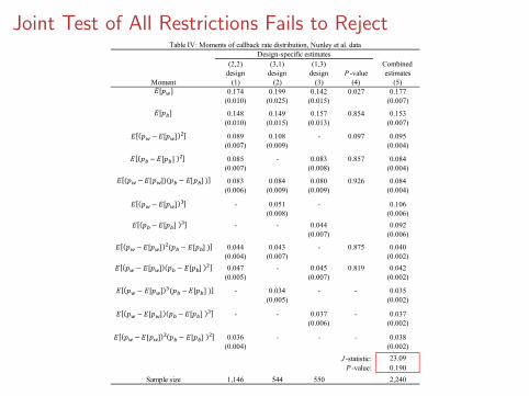
Joint Test of All Restrictions Fails to Reject

(2,2) (3,1) (1,3) Combineddesign design design P -value estimates

Moment (1) (2) (3) (4) (5)0.174 0.199 0.142 0.027 0.177

(0.010) (0.025) (0.015) (0.007)

0.148 0.149 0.157 0.854 0.153(0.010) (0.015) (0.013) (0.007)

0.089 0.108 - 0.097 0.095(0.007) (0.009) (0.004)

0.085 - 0.083 0.857 0.084(0.007) (0.008) (0.004)

0.083 0.084 0.080 0.926 0.084(0.006) (0.009) (0.009) (0.004)

- 0.051 - 0.106(0.008) (0.006)

- - 0.044 0.092(0.007) (0.006)

0.044 0.043 - 0.875 0.040(0.004) (0.007) (0.002)0.047 - 0.045 0.819 0.042

(0.005) (0.007) (0.002)

- 0.034 - - 0.035(0.005) (0.002)

- - 0.037 - 0.037(0.006) (0.002)

0.036 - - - 0.038(0.004) (0.002)0

23.090.190

Sample size 1,146 544 550 2,240

Table IV: Moments of callback rate distribution, Nunley et al. dataDesign-specific estimates

J -statistic:P -value:

𝐸[𝑝$]

𝐸[𝑝&]

𝐸 𝑝$ −𝐸[𝑝$] (

𝐸 𝑝& −𝐸[𝑝&] (

𝐸 (𝑝$ −𝐸[𝑝$])(𝑝& − 𝐸[𝑝&] )

𝐸 𝑝$ −𝐸[𝑝$] +

𝐸 𝑝& −𝐸[𝑝&] +

𝐸 𝑝$ −𝐸[𝑝$] ((𝑝& − 𝐸[𝑝&] )

𝐸 𝑝$ − 𝐸[𝑝$] 𝑝& − 𝐸[𝑝&] (

𝐸 𝑝$ − 𝐸[𝑝$] +(𝑝& −𝐸[𝑝&] )

𝐸 𝑝$ −𝐸[𝑝$] 𝑝& −𝐸[𝑝&] +

𝐸 𝑝$ −𝐸[𝑝$] ( 𝑝& − 𝐸[𝑝&] (

Treatment Effects Are Variable and Skewed

p b p w p b - p w

(1) (2) (3)Mean 0.153 0.177 -0.023

(0.007) (0.007) (0.005)


Correlation with p w 0.944 1.000 -0.336(0.018) - (0.048)

Skewness 3.757 3.648 -4.450(0.074) (0.087) (0.405)

Table VI.B: Treatment effect variation in Nunley et al. (2015)

Thick Tail of Extreme Discriminators in AGCV

p m p f p m - p f

(1) (2) (3)Mean 0.114 0.140 -0.025

(0.009) (0.009) (0.008)


Correlation with p f 0.735 1.000 -0.483(0.035) - (0.051)

Skewness 4.067 3.748 -1.403(0.140) (1.161) (0.385)

Excess kurtosis 8.452 5.756 12.227(1.458) (8.790) (2.291)

Table VI.C: Treatment effect variation in AGCV

Prevalence and Posteriors

In BM, At Least 13% of Jobs Discriminate

Sharediscriminating:

Pr(p w ≠ p b )(1)

0.130J -statistic: 29.26

P -value (bound = 0): 0.000

Lower bounds on discrimination probabilities, BM data

At Least 44% Making Two Total Calls Discriminate

Sharediscriminating:

Pr(p w ≠ p b )Callbacks (1)

All 0.1300 0.038

1 0.424

2 0.442

3 0.508

4 0.212J -statistic: 29.26

P -value (bound = 0): 0.000


Cannot Reject Absence of Discrimination Against Whites

Share Share disc. Share disc.discriminating: against whites: against blacks:

Pr(p w ≠ p b ) Pr(p w < p b ) Pr(p b < p w )Callbacks (1) (2) (3)

All 0.130 0.000 0.1300 0.038 0.000 0.038

1 0.424 0.000 0.424

2 0.442 0.000 0.442

3 0.508 0.000 0.508

4 0.212 0.000 0.212J -statistic: 29.26 0.00 29.26

P -value (bound = 0): 0.000 1.000 0.000


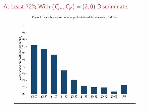
At Least 72% With (Cjw ,Cjb) = (2, 0) Discriminate

Figure I: Lower bounds on posterior probabilities of discrimination, BM data

In Nunley et al., Cannot Reject Pr(pjw < pjb) = 0



All 0.358 0.154 0.1730 0.152 0.093 0.048

1 0.672 0.185 0.433

2 0.691 0.016 0.675

3 0.821 0.067 0.736

4 0.421 0.257 0.128J -statistic: 62.64 23.46 62.64

P -value (bound = 0): 0.000 0.120 0.000

Lower bounds on discrimination probabilities, Nunley et al. data

At Least 68% That Make Two Calls Have pjb < pjw



All 0.358 0.154 0.1730 0.152 0.093 0.048

1 0.672 0.185 0.433

2 0.691 0.016 0.675

3 0.821 0.067 0.736

4 0.421 0.257 0.128J -statistic: 62.64 23.46 62.64

P -value (bound = 0): 0.000 0.120 0.000

Lower bounds on discrimination probabilities, Nunley et al. data

Lower Bounds on Posteriors Above 85%

Figure II: Lower bounds on posterior probabilities of discrimination, Nunley et al. data

In AGCV, Discrimination Against Both Men and Women

Share Share disc. Share disc.discriminating: against women: against men:

Pr(p f ≠ p m ) Pr(p f < p m ) Pr(p f < p m )Callbacks (1) (2) (3)

All 0.277 0.089 0.1880 0.136 0.040 0.095

1 0.895 0.414 0.480

2 0.716 0.260 0.456

3 0.576 0.047 0.528

4 0.503 0.055 0.447

5 0.346 0.171 0.1756 0.409 0.212 0.1977 0.486 0.157 0.3298 0.076 0.011 0.065J -statistic: 369.66 33.88 359.95

P -value (bound = 0): 0.000 0.005 0.000

Lower bounds on discrimination probabilities, AGCV data

Lower Bounds on Posteriors Above 90%

Figure III: Lower bounds on posterior probabilities of discrimination, AGCV data

Detection Error Tradeoffs

Experimental Design and Detection Error Tradeoffs

Results so far establish that some callback patterns produce high posteriorprobabilities of discrimination even with few applications per job

I But few jobs produce these patterns. Can correspondence experimentsserve as a useful tool for detecting discrimination when prevalence is low?

I Consider alternative hypothetical experiments based on models fit to theNunley et al. (2015) data

I Take the perspective of hypothetical regulator who knows G(·, ·) andmust decide which jobs to investigate based upon callbacks

I Investigations are costly, want to detect most extremediscriminators

I Start with a parametric model for G(·, ·) then ask how regulator’sdecisions are affected by second-guessing parametric assumptions

I Detection/error tradeoff (DET) curves: tradeoff between truenegatives and true positives for a fixed number of apps

Mixed Logit

Logit model for callback to application ` at job j :

Pr (Yj` = 1|αj , βj ,Rj`,Xj`) = Λ(αj − βj1{Rj` = b}+ X ′j`ψ

).

I Λ(x) ≡ exp(x)/(1 + exp(x)) is the logistic CDF

I Rj` indicates race, Xj` includes other randomly-assignedcharacteristics (GPA, experience, etc.)

I Two-type mixing:

αj ∼ N(α0, σ

2α

),

βj =

{β0, with prob. Λ(τ0 + τααj),

0, with prob. 1− Λ(τ0 + τααj).

Discrimination is Rare But Intense

Constant No selection Selection(1) (2) (3)

Distribution of logit(pw): 𝛼0 -4.708 -4.931 -4.927(0.223) (0.242) (0.280)

𝜎𝛼 4.745 4.988 4.983(0.223) (0.249) (0.294)

Discrimination intensity: 𝛽0 0.456 4.046 4.053(0.108) (1.563) (1.576)

Discrimination logit: 𝜏0 - -1.586 -1.556(0.416) (1.098)

𝜏𝛼 - - -0.005(0.180)

Fraction with p w ≠ p b : 1.000 0.168 0.170

Log-likelihood -2,792.1 -2,788.2 -2,788.2Parameters 15 16 17Sample size 2,305 2,305 2,305

Table X: Mixed logit estimates, Nunley et al. dataTypes

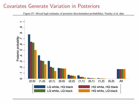
Covariates Generate Variation in PosteriorsFigure IV: Mixed logit estimates of posterior discrimination probabilities, Nunley et al. data

Regulator’s Problem

Consider a regulator who knows G and must choose whether to investigate,δj ∈ {0, 1}, based upon callbacks (Cjw ,Cjb)

I Regulator seeks to minimize loss function:

Lj(δj) = δj ×(κ− Λ

(Λ−1(pjw )− Λ−1(pjb)

))I Intuitively, the regulator wants to investigate employers with large logit

coefficients

Optimal decision rule δ(Cjb,Cjw ) minimizes expected loss (risk)

R(G , δ) ≡ E[Lj(δ(Cjw ,Cjb))]

I In the two-type mixed logit, this results in a posterior cutoff rule:

δ(Cjw ,Cjb) = 1

{P(Cjw ,Cjb,G(., .)) >

κ− 1/2

Λ(β0)− 1/2

}I Focus on example where κ is such that posterior cutoff is 80%.

With 2 Pairs, 80% Threshold Yields Few Investigations

Figure V: Detection/error tradeoffs, NPRS data

.988

.99

.992

.994

.996

.998

1Sh

are

of n

on-d

iscrim

inat

ors

not i

nves

tigat

ed

0 .05 .1 .15Share of discriminators investigated

2 pairs

Sending 5 Pairs Boosts Detection Substantially


.988

.99

.992

.994

.996

.998

1Sh

are

of n

on-d

iscrim

inat

ors

not i

nves

tigat

ed


2 pairs 5 pairs

Leveraging Covariates Yields Further Gains


.988

.99

.992

.994

.996

.998

1Sh

are

of n

on-d

iscrim

inat

ors

not i

nves

tigat

ed


2 pairs 5 pairs5 pairs (HQ black, LQ white)

Fixing Size at 0.01 Yields More (Mostly False) AccusationsFigure V: Detection/error tradeoffs, NPRS data

.988

.99

.992

.994

.996

.998

1Sh

are

of n

on-d

iscrim

inat

ors

not i

nves

tigat

ed


2 pairs 5 pairs5 pairs (HQ black, LQ white)

Accommodating Ambiguity

Beyond Logit: Policy When Partially Identified

How would decisions change if the regulator fears that G(·, ·) is not logit?

I Important (extreme) benchmark for decisionmaking under ambiguity:minimax decision rule

I Max risk function and minimax decision rule when auditor knows G lies insome identified set Θ:

Rm(Θ, δ) ≡ supG∈Θ

R(G , δ), δmm ≡ arg infδRm(Θ, δ)

I Minimax regulator chooses δmm to minimize risk, assuming nature willselect the least favorable distribution in Θ in response to any decision rule(“Γ-minimax”)

I Manage space of decision rules by considering a restricted set defined bylogit posterior cutoffs

I Contrast risk and decisions based upon mixed logit prior and minimaxdetails

Minimax Regulator Chooses Slightly Higher Threshold(intuition: risk function nearly identified for rules using high posterior cutoffs)

Figure VI: Bayes and minimax risk, NPRS data

Notes: This figure displays risk functions generated by a hypothetical experiment sending five white and five black applications to jobs in the population studied by Nunley et al. (2015). Resumes are randomly assigned to high or low quality with equal probability, where quality is defined as +/-1 the empirical standard deviation of the logit covariate index. The horizontal axis plots the posterior threshold at which jobs are accused of discrimination. The grey curve displays risk based on the logit data generating process in column (2) of Table V. The cost of an investigation is calibrated so that a Bayesian regulator sets the posterior cutoff at 0.8. The blue curve plots minimax risk calculated by choosing the joint distribution of callback probabilities to maximize risk for each decision rule subject to the moments identified by the Nunley et al. (2015) experiment, restricted to decision rules that order jobs by the logit posterior threshold. Vertical lines indicate risk-minimizing thresholds. The window displays logit and minimax risk at threesholds of 0.75 and above, with risk-minimizing points indicated in red.

Concluding Thoughts

I Tremendous heterogeneity in discrimination ⇒ enforcing equalopportunity is a difficult inferential problemI Results today suggest favorable detection rates achievable with

minor modifications to standard audit designs

I Ongoing workI Jobs vs firms: is bad behavior clustered in particular

companies? How to construct reliable rankings?I Optimal experimental design: dynamic auditing to detect

effects at lower cost

I Methods applicable to other settings where behavioral responses ofindividual units are of interest. Examples:I Workplace safety audits (Levine et al., 2012)

I Choice experiments (Halevy et al., 2018)

I Group testing for immunity (Dorfman, 1943; Gollier, 2020)

Discretization of G

I We approximate G(pw , pb) with the discrete distribution:

GK (pw , pb) =K∑

k=1

K∑l=1

ηkl1 {pw ≤ % (k, l) , pb ≤ % (l , k)}

I {ηkl}K ,Kk=1,l=1 are probability masses

I {% (k, l) , % (l , k)}K ,Kk=1,l=1 are a set of mass point coordinates generated by

% (x , y) =min {x , y} − 1

K︸︷︷︸diagonal

+max {0, x − y}2

K (1 + K − y)︸︷︷︸off-diagonal

.

I Gives a two-dimensional grid with K 2 elements, equally spaced along thediagonal and quadratically spaced off the diagonal according to distancefrom diagonal

Shape Constrained GMM

I Let f denote vector of empirical callback frequencies

I Shape constrained GMM estimator of η solves quadratic programmingproblem:

η = arg infη

(f − BMη)′W (f − BMη) s.t. η ≥ 0, 1′η = 1.

I M is a dim(µ)× K 2 matrix defined so that Mη = µ for GK

I Yields shape constrained moment estimates: µ = M η

I W is weighting matrix – use two-step optimal weighting

I Set K = 150 for GMM estimation

back

Hong and Li (2017) Standard Errors

I Bootstrap µ∗ solves QP problem replacing f with (f + J−1/4f ∗), whereelements of f ∗ given by:

√J[∑

j ω∗j 1{Cjw =cw ,Cjb=cb}∑

j ω∗j

−∑

j 1{Cjw =cw ,Cjb=cb}J

].

I Weights ω∗j drawn iid from exponential distribution with mean 0 andvariance 1

I Standard errors for φ(µ) computed as standard deviation ofJ−1/4[φ(µ∗)− φ(µ)] across bootstrap replications

back

Chernozhukov et al. (2015) Goodness of Fit Test

I “J-test” goodness of fit statistic:

Tn = infη

(f − BMη)′Σ−1(f − BMη) s.t. η ≥ 0, 1′η = 1

I Letting F ∗ denote (centered) bootstrap analogue of f and W ∗ aweighting matrix, bootstrap test statistic is

T ∗n = infπ,h

(F ∗ − BMη)′W ∗(F ∗ − BMη)

s.t. (f − BMη)′W (f − BMη) = Tn, η ≥ 0, 1′η = 1, h ≥ −η, 1′h = 0.

I As in the full sample, conduct two-step GMM estimation in bootstrapreplications

I Calculate p-value as fraction of bootstrap samples with T ∗n > Tn

I Solve via Second Order Cone Programming

back

Testing for Dependence Across TrialsI Consider set of Jk jobs making k total calls

I Under the null of iid trials, all sequences yielding k successes are equallylikely

I With L = 4 and k = 2, six possible sequences: (1,1,0,0), (1,0,1,0),(1,0,0,1), (0,1,1,0), (0,1,0,1), (0,0,1,1)

I Test statistic:

Tk =

q−1k∑s=1

(qs,k − qk)2

qk(1− qk)/Jk

I qs,k is empirical frequency of sequence s among those with k calls,

qk =

(Lk

)−1

is expected frequency under the null

I Under the null Tk is χ2 distributed with

(Lk

)− 1 degrees of freedom

back

Importance of πt

I Define the t-conditional quantities where t = cw + cb is total callbacks

(pwj , pbj) |Cwj + Cbj = t ∼ Gt (·, ·)

ft(cw ) =f (cw , t − cw )∑Lwx=0 f (x , t − x)

ft(cw |pw , pb) =f (cw , t − cw |pw , pb)∑Lwx=0 f (x , t − x |pw , pb)

I Note by standard sufficiency arguments that

ft(cw |p, p) =

(Lw

cw

)(Lb

t − cw

)(

Lt

) = B (t, cw )

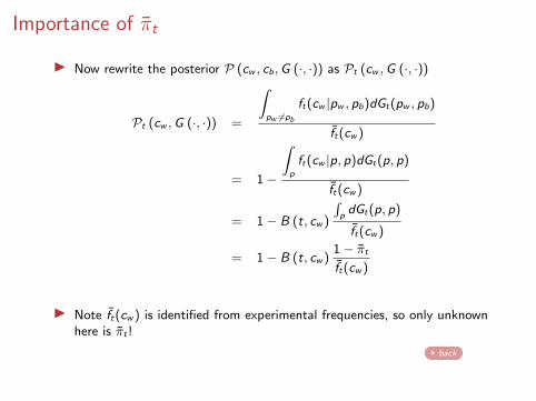
Importance of πt

I Now rewrite the posterior P (cw , cb,G (·, ·)) as Pt (cw ,G (·, ·))

Pt (cw ,G (·, ·)) =

∫pw 6=pb

ft(cw |pw , pb)dGt(pw , pb)

ft(cw )

= 1−

∫p

ft(cw |p, p)dGt(p, p)

ft(cw )

= 1− B (t, cw )

∫pdGt(p, p)

ft(cw )

= 1− B (t, cw )1− πt

ft(cw )

I Note ft(cw ) is identified from experimental frequencies, so only unknownhere is πt !

back

Linear Programming

I Optimization problem for computing lower bound on share discriminating:

max{ηkl}

K∑l=1

K∑k=1

ηkl1{%(k, l) = %(l , k)} s.t.K∑

k=1

K∑l=1

ηkl = 1, ηkl ≥ 0

I Additional moment constraints for all (cw , cb):

f (cw , cb) =

(Lw

cw

)(Lb

cb

)∑Kk=1

∑Kl=1 ηkl

×% (k, l)cw (1− % (k, l))Lw−cw % (l , k)cb (1− % (l , k))Lb−cb .

I Set K = 900 for computing bounds

back

Computing Maximum RiskI Letting H and L refer to high and low quality covariate values, we approximate

G(pHw , pLw , p

Hb , p

Lb ) with

GK (pHw , pLw , p

Hb , p

Lb ) =

K∑k=1

K∑l=1

K∑k′=1

K∑l′=1

ηklk′ l′

×1{pHw ≤ % (k, l) , pLw ≤ % (k ′, l ′) , pHb ≤ % (l , k) , pLb ≤ % (l ′, k ′)

}.

I Maximal risk function for posterior cutoff q:

RmJ (q) =

J max{ηklk′ l′}

∑l∈A1

wlE

δ(Cj , l , q)

κ− Λ

∑x∈{H,L)

Λ−1(pxwj )−Λ−1(pxbj )

2

|Lj = l

I A1 is list of possible quality configurations with corresponding probabilities wa

I Constraints: ηklk′ l′ positive and sum to 1, along with matching a list oflogit-smoothed callback frequencies

I Joint probabilities Pr(δ(Cj , a, q

)= 1,Dj = d

)linear in ηklk′ l′ (see Appendix D)

I Set K = 30 when computing maximal risk in practice

back

reasonable doubt: experimental detection of job …pkline/papers/rd_slides.pdfreasonable doubt:...

Documents