reasoning under uncertainty: introduction to probability
TRANSCRIPT

Reasoning Under Uncertainty: Introduction to Probability
Alan Mackworth
UBC CS 322 – Uncertainty 1
March 11, 2013
Textbook §6.1, 6.1.1, 6.1.3

Coloured Cards
• If you lost/forgot your set, please come to the front and pick up a new one – We’ll use them quite a bit in the uncertainty module
2

Lecture Overview
• Reasoning Under Uncertainty – Motivation – Introduction to Probability
• Random Variables and Possible World Semantics • Probability Distributions and Marginalization • Time-permitting: Conditioning
3

4
Course Overview Environment
Problem Type
Logic
Planning
Deterministic Stochastic
Constraint Satisfaction Search
Arc Consistency
Search
Search
Logics
STRIPS
Variables + Constraints
Variable Elimination
Bayesian Networks
Decision Networks
Markov Processes
Static
Sequential
Representation Reasoning Technique
Uncertainty
Decision Theory
Course Module
Variable Elimination
Value Iteration
Planning
For the rest of the course, we will consider uncertainty
As CSP (using arc consistency)

Lecture Overview • Reasoning Under Uncertainty
– Motivation – Introduction to Probability
• Random Variables and Possible World Semantics • Probability Distributions and Marginalization • Time-permitting: Conditioning
5

Two main sources of uncertainty (From Lecture 2) • Sensing Uncertainty: The agent cannot fully observe a state
of interest. For example:
– Right now, how many people are in this room? In this building? – What disease does this patient have? – Where is the soccer player behind me?
• Effect Uncertainty: The agent cannot be certain about the effects of its actions.
For example: – If I work hard, will I get an A? – Will this drug work for this patient? – Where will the ball go when I kick it?

Motivation for uncertainty
• To act in the real world, we almost always have to handle uncertainty (both effect and sensing uncertainty) – Deterministic domains are an abstraction
• Sometimes this abstraction enables more powerful inference – Now we don’t make this abstraction anymore
• Our representation becomes more expressive and general
• AI main focus shifted from logic to probability in the 1980s – The language of probability is very expressive and general – New representations enable efficient reasoning
• We will see some of these, in particular Bayesian networks – Reasoning under uncertainty is part of the ‘new’ AI – This is not a dichotomy: framework for probability is logical! – New frontier: combine logic and probability
7

Interesting article about AI and uncertainty • “The machine age”
– by Peter Norvig (head of research at Google) – New York Post, 12 February 2011 – http://www.nypost.com/f/print/news/opinion/opedcolumnists/
the_machine_age_tM7xPAv4pI4JslK0M1JtxI
– “The things we thought were hard turned out to be easier.” • Playing grandmaster level chess,
or proving theorems in integral calculus – “Tasks that we at first thought were easy turned out to be hard.”
• A toddler (or a dog) can distinguish hundreds of objects (ball, bottle, blanket, mother, …) just by glancing at them
• Very difficult for computer vision to perform at this level – “Dealing with uncertainty turned out to be more important than
thinking with logical precision.” • Reasoning under uncertainty (and lots of data) are key to progress
8

Lecture Overview
• Reasoning Under Uncertainty – Motivation – Introduction to Probability
• Random Variables and Possible World Semantics • Probability Distributions and Marginalization • Time-permitting: Conditioning
9

Probability as a formal measure of uncertainty (ignorance)
• Probability measures an agent's degree of belief in propositions about states of the world – It does not measure how true a proposition is. – Propositions are true or false. We simply may not know exactly which. – Example:
• I roll a fair dice. What is the probability that the result is a ‘6’?

Probability as a formal measure of uncertainty (ignorance)
• Probability measures an agent's degree of belief in truth of propositions about states of the world – It does not measure how true a proposition is – Propositions are true or false. We simply may not know exactly which. – Example:
• I roll a fair dice. What is ‘the’ (my) probability that the result is a ‘6’? – It is 1/6 ≈ 16.7%. – The result is either a ‘6’ or not. But I don’t know which one.
• I now look at the dice. What is ‘the’ (my) probability now? – Your probability hasn’t changed: 1/6 ≈ 16.7% – My probability is now either 1 or 0, depending on what I observed.
• What if I tell some of you the result is even? – Their probability increases to 1/3 ≈ 33.3%
(assuming they believe I speak the truth) • Different agents can have different degrees of belief in (probabilities for) a
proposition conditioned on the evidence they have.

Probability as a formal measure of uncertainty/ignorance
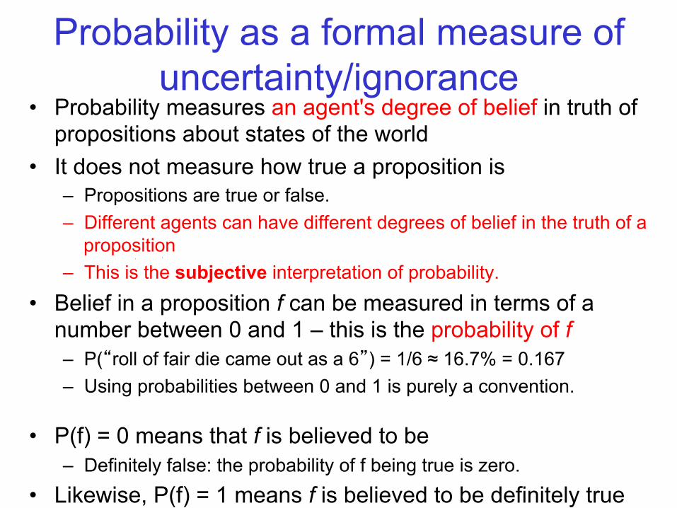
• Probability measures an agent's degree of belief in truth of propositions about states of the world
• It does not measure how true a proposition is – Propositions are true or false. – Different agents can have different degrees of belief in the truth of a
proposition – This is the subjective interpretation of probability.
• Belief in a proposition f can be measured in terms of a number between 0 and 1 – this is the probability of f – P(“roll of fair die came out as a 6”) = 1/6 ≈ 16.7% = 0.167 – Using probabilities between 0 and 1 is purely a convention.
• P(f) = 0 means that f is believed to be
Probably false Probably true Definitely false Definitely true
Probability as a formal measure of uncertainty/ignorance
• Probability measures an agent's degree of belief in truth of propositions about states of the world
• It does not measure how true a proposition is – Propositions are true or false. – Different agents can have different degrees of belief in the truth of a
proposition – This is the subjective interpretation of probability.
• Belief in a proposition f can be measured in terms of a number between 0 and 1 – this is the probability of f – P(“roll of fair die came out as a 6”) = 1/6 ≈ 16.7% = 0.167 – Using probabilities between 0 and 1 is purely a convention.
• P(f) = 0 means that f is believed to be – Definitely false: the probability of f being true is zero.
• Likewise, P(f) = 1 means f is believed to be definitely true

Probability Theory and Random Variables • Probability Theory: system of logical axioms and formal
operations for sound reasoning under uncertainty
• Basic element: random variable X – X is a variable like the ones we have seen in CSP/Planning/Logic, but
the agent can be uncertain about the value of X – As usual, the domain of a random variable X, written dom(X), is the
set of values X can take
• Types of variables – Boolean: e.g., Cancer (does the patient have cancer or not?) – Categorical: e.g., CancerType could be one of {breastCancer,
lungCancer, skinMelanomas} – Numeric: e.g., Temperature (integer or real)
– We will focus on Boolean and categorical variables

Possible Worlds Semantics
• Example: if we model only 2 Boolean variables Smoking and Cancer, how many distinct possible worlds are there?
• A possible world w specifies an assignment to each random variable

Possible Worlds Semantics
• Example: if we model only 2 Boolean variables Smoking and Cancer. Then there are 22=4 distinct possible worlds:
w1: Smoking = T ∧ Cancer = T w2: Smoking = T ∧ Cancer = F w3: Smoking = F ∧ Cancer = T w4: Smoking = T ∧ Cancer = T
• A possible world w specifies an assignment to each random variable
• w ⊧ X=x means variable X is assigned value x in world w • Define a nonnegative measure µ(w) on possible worlds w
such that the measures on the possible worlds sum to 1 - The probability of proposition f is defined by:
Smoking ! Cancer!
T" T"T" F"F" T"F" F"

Possible Worlds Semantics
w ⊧ X=x means variable X is assigned value x in world w
- Probability measure µ(w) sums to 1 over all possible worlds w
- The probability of proposition f is defined by:
• New example: weather in Vancouver – Modeled as one Boolean variable:
• Weather with domain {sunny, cloudy} – Possible worlds:
w1: Weather = sunny w2: Weather = cloudy
• Let’s say the probability of sunny weather is 0.4 – I.e. p(Weather = sunny) = 0.4 – What is the probability of p(Weather = cloudy)?
0.4 We don’t have enough information to compute that probability 1 0.6
Weather! p!
sunny" 0.4"cloudy"

Possible Worlds Semantics
w ⊧ X=x means variable X is assigned value x in world w
- Probability measure µ(w) sums to 1 over all possible worlds w
- The probability of proposition f is defined by:
Weather! p!
sunny" 0.4"cloudy" 0.6!
• New example: weather in Vancouver – Modeled as one categorical variable:
• Weather with domain {sunny, cloudy} – Possible worlds:
w1: Weather = sunny w2: Weather = cloudy
• Let’s say the probability of sunny weather is 0.4 – I.e. p(Weather = sunny) = 0.4 – What is the probability of p(Weather = cloudy)?
• p(Weather = sunny) = 0.4 means that µ(w1) is 0.4 • µ(w1) and µ(w2) have to sum to 1 (those are the only 2 possible worlds) • So µ(w2) has to be 0.6, and thus p(Weather = cloudy) = 0.6

One more example • Now we have an additional variable:
– Temperature, modeled as a categorical variable with domain {hot, mild, cold}
– There are now 6 possible worlds:
– What’s the probability of it being cloudy and cold?
• Hint: 0.10 + 0.20 + 0.10 + 0.05 + 0.35 = 0.8
0.2 0.1 0.3 1
Weather! Temperature! µ(w)!sunny hot" 0.10"sunny mild" 0.20"sunny cold" 0.10"cloudy hot" 0.05"cloudy mild" 0.35"cloudy cold" ?"

One more example • Now we have an additional variable:
– Temperature, modeled as a categorical variable with domain {hot, mild, cold}
– There are now 6 possible worlds:
– What’s the probability of it being cloudy and cold?
• It is 0.2: the probability has to sum to 1 over all possible worlds
Weather! Temperature! µ(w)!sunny hot" 0.10"sunny mild" 0.20"sunny cold" 0.10"cloudy hot" 0.05"cloudy mild" 0.35"cloudy cold" 0.2!

Lecture Overview • Reasoning Under Uncertainty
– Motivation – Introduction to Probability
• Random Variables and Possible World Semantics • Probability Distributions and Marginalization • Time-permitting: Conditioning
21

Probability Distributions
Consider the case where possible worlds are simply assignments to one random variable.
– When dom(X) is infinite we need a probability density function – We will focus on the finite case
22
Definition (probability distribution) A probability distribution P on a random variable X is a function dom(X) → [0,1] such that
x → P(X=x)

Joint Distribution • The joint distribution over random variables X1, …, Xn:
– a probability distribution over the joint random variable <X1, …, Xn> with domain dom(X1) × … × dom(Xn) (the Cartesian product)
• Example from before – Joint probability distribution
over random variables Weather and Temperature
– Each row corresponds to an assignment of values to these variables, and the probability of this joint assignment
– In general, each row corresponds to an assignment X1= x1, …, Xn= xn and its probability P(X1= x1, … ,Xn= xn)
– We also write P(X1= x1 ∧ … ∧ Xn= xn) – The sum of probabilities across the whole table is 1.
23
Weather! Temperature! µ(w)!sunny hot" 0.10"sunny mild" 0.20"sunny cold" 0.10"cloudy hot" 0.05"cloudy mild" 0.35"cloudy cold" 0.20"

Marginalization • Given the joint distribution, we can compute distributions
over smaller sets of variables through marginalization:
P(X=x) = Σz∈dom(Z) P(X=x, Z = z)
– We also write this as P(X) = Σz∈dom(Z) P(X, Z = z).
• This corresponds to summing out a dimension in the table. • The new table still sums to 1. It must, since it’s a probability distribution!
24
Temperature! µ(w)!hot ?"mild ?"cold ?"
Weather! Temperature! µ(w)!sunny hot" 0.10"sunny mild" 0.20"sunny cold" 0.10"cloudy hot" 0.05"cloudy mild" 0.35"cloudy cold" 0.20"

Marginalization • Given the joint distribution, we can compute distributions
over smaller sets of variables through marginalization:
P(X=x) = Σz∈dom(Z) P(X=x, Z = z)
– We also write this as P(X) = Σz∈dom(Z) P(X, Z = z).
• This corresponds to summing out a dimension in the table. • The new table still sums to 1. It must, since it’s a probability distribution!
25
Temperature! µ(w)!hot ??"mild cold
Weather! Temperature! µ(w)!sunny hot" 0.10"sunny mild" 0.20"sunny cold" 0.10"cloudy hot" 0.05"cloudy mild" 0.35"cloudy cold" 0.20"
P(Temperature=hot) = P(Weather=sunny, Temperature = hot) + P(Weather=cloudy, Temperature = hot) = 0.10 + 0.05 = 0.15

Marginalization • Given the joint distribution, we can compute distributions
over smaller sets of variables through marginalization:
P(X=x) = Σz∈dom(Z) P(X=x, Z = z)
– We also write this as P(X) = Σz∈dom(Z) P(X, Z = z).
• This corresponds to summing out a dimension in the table. • The new table still sums to 1. It must, since it’s a probability distribution!
26
Temperature! µ(w)!hot 0.15"mild cold
Weather! Temperature! µ(w)!sunny hot" 0.10"sunny mild" 0.20"sunny cold" 0.10"cloudy hot" 0.05"cloudy mild" 0.35"cloudy cold" 0.20"
P(Temperature=hot) = P(Weather=sunny, Temperature = hot) + P(Weather=cloudy, Temperature = hot) = 0.10 + 0.05 = 0.15

Marginalization • Given the joint distribution, we can compute distributions
over smaller sets of variables through marginalization:
P(X=x) = Σz∈dom(Z) P(X=x, Z = z)
– We also write this as P(X) = Σz∈dom(Z) P(X, Z = z).
• This corresponds to summing out a dimension in the table. • The new table still sums to 1. It must, since it’s a probability distribution!
Temperature! µ(w)!hot 0.15"mild ??"cold
Weather! Temperature! µ(w)!sunny hot" 0.10"sunny mild" 0.20"sunny cold" 0.10"cloudy hot" 0.05"cloudy mild" 0.35"cloudy cold" 0.20"
0.35 0.20 0.85 0.55
27
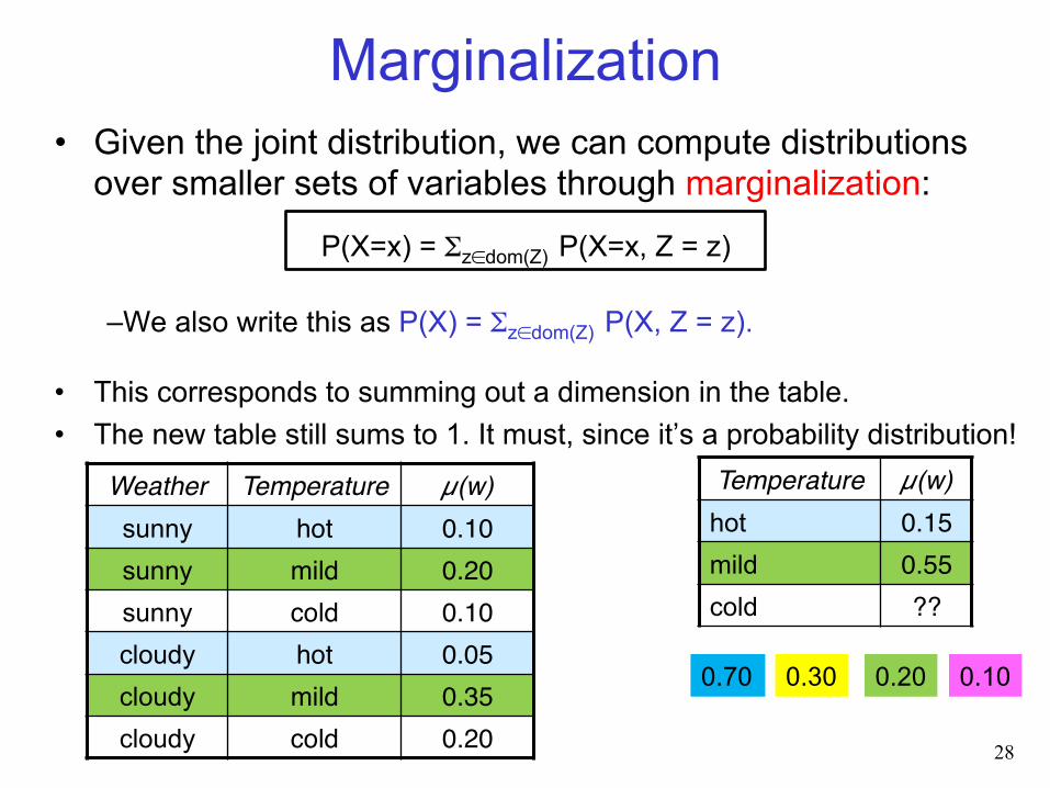
Marginalization • Given the joint distribution, we can compute distributions
over smaller sets of variables through marginalization:
P(X=x) = Σz∈dom(Z) P(X=x, Z = z)
– We also write this as P(X) = Σz∈dom(Z) P(X, Z = z).
• This corresponds to summing out a dimension in the table. • The new table still sums to 1. It must, since it’s a probability distribution!
Temperature! µ(w)!hot 0.15"mild 0.55"cold ??"
Weather! Temperature! µ(w)!sunny hot" 0.10"sunny mild" 0.20"sunny cold" 0.10"cloudy hot" 0.05"cloudy mild" 0.35"cloudy cold" 0.20"
0.30 0.70 0.20 0.10
28

Marginalization • Given the joint distribution, we can compute distributions
over smaller sets of variables through marginalization:
P(X=x) = Σz∈dom(Z) P(X=x, Z = z)
– We also write this as P(X) = Σz∈dom(Z) P(X, Z = z).
• This corresponds to summing out a dimension in the table. • The new table still sums to 1. It must, since it’s a probability distribution!
29
Temperature! µ(w)!hot 0.15"mild 0.55"cold 0.30"
Weather! Temperature! µ(w)!sunny hot" 0.10"sunny mild" 0.20"sunny cold" 0.10"cloudy hot" 0.05"cloudy mild" 0.35"cloudy cold" 0.20"
Alternative way to compute last entry: probabilities have to sum to 1.

Marginalization • Given the joint distribution, we can compute distributions
over smaller sets of variables through marginalization:
P(X=x) = Σz∈dom(Z) P(X=x, Z = z)
– We also write this as P(X) = Σz∈dom(Z) P(X, Z = z).
• You can marginalize out any of the variables
30
Weather! µ(w)!sunny 0.40"cloudy
Weather! Temperature! µ(w)!sunny hot" 0.10"sunny mild" 0.20"sunny cold" 0.10"cloudy hot" 0.05"cloudy mild" 0.35"cloudy cold" 0.20"
P(Weather=sunny) = P(Weather=sunny, Temperature = hot) + P(Weather=sunny, Temperature = mild) + P(Weather=sunny, Temperature = cold) = 0.10 + 0.20 + 0.10 = 0.40
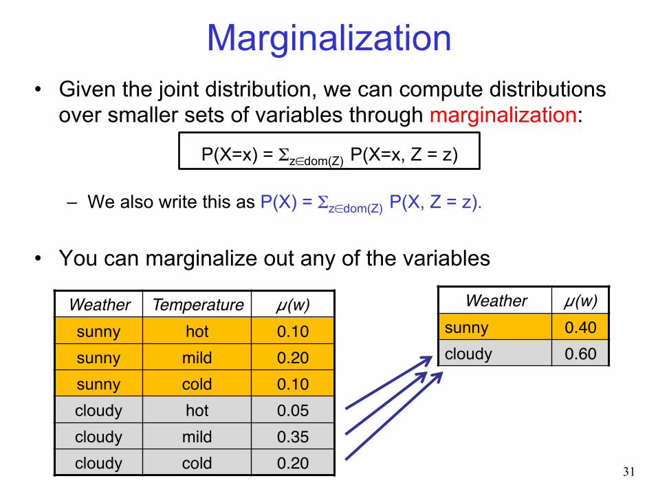
Marginalization • Given the joint distribution, we can compute distributions
over smaller sets of variables through marginalization:
P(X=x) = Σz∈dom(Z) P(X=x, Z = z)
– We also write this as P(X) = Σz∈dom(Z) P(X, Z = z).
• You can marginalize out any of the variables
31
Weather! µ(w)!sunny 0.40"cloudy 0.60"
Weather! Temperature! µ(w)!sunny hot" 0.10"sunny mild" 0.20"sunny cold" 0.10"cloudy hot" 0.05"cloudy mild" 0.35"cloudy cold" 0.20"

Marginalization • We can also marginalize out more than one variable at once
P(X=x) = Σz1∈dom(Z1),…, zn∈dom(Zn) P(X=x, Z1 = z1, …, Zn = zn)
32
Weather! µ(w)!sunny 0.40"cloudy
Wind! Weather! Temperature! µ(w)!yes sunny hot" 0.04"yes sunny mild" 0.09"yes sunny cold" 0.07"yes cloudy hot" 0.01"yes cloudy mild" 0.10"yes cloudy cold" 0.12"no sunny hot" 0.06"no sunny mild" 0.11"no sunny cold" 0.03"no cloudy hot" 0.04"no cloudy mild" 0.25"no cloudy cold" 0.08"
Marginalizing out variables Wind and Temperature, i.e. those are the ones being removed from the distribution
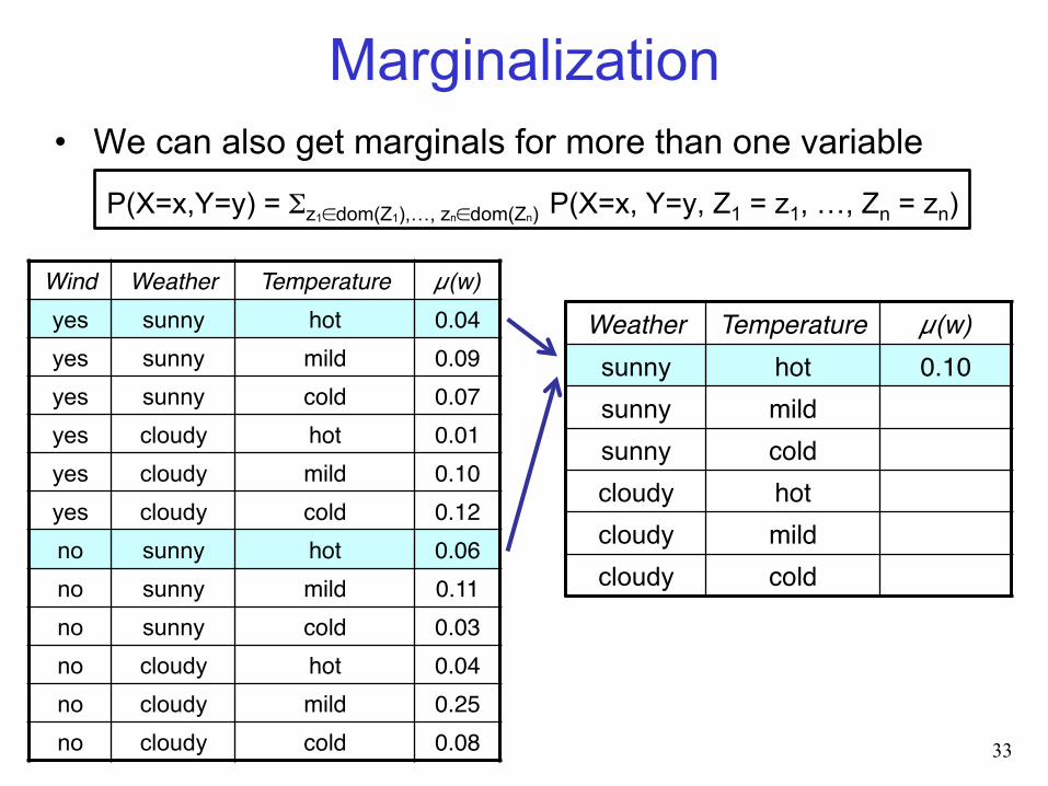
Marginalization • We can also get marginals for more than one variable
P(X=x,Y=y) = Σz1∈dom(Z1),…, zn∈dom(Zn) P(X=x, Y=y, Z1 = z1, …, Zn = zn)
33
Wind! Weather! Temperature! µ(w)!yes sunny hot" 0.04"yes sunny mild" 0.09"yes sunny cold" 0.07"yes cloudy hot" 0.01"yes cloudy mild" 0.10"yes cloudy cold" 0.12"no sunny hot" 0.06"no sunny mild" 0.11"no sunny cold" 0.03"no cloudy hot" 0.04"no cloudy mild" 0.25"no cloudy cold" 0.08"
Weather! Temperature! µ(w)!sunny hot" 0.10"sunny mild"sunny cold"cloudy hot"cloudy mild"cloudy cold"

• Define and give examples of random variables, their domains and probability distributions
• Calculate the probability of a proposition f given µ(w) for the set of possible worlds
• Define a joint probability distribution (JPD) • Given a JPD
– Marginalize over specific variables – Compute distributions over any subset of the variables
• Heads up: study these concepts, especially marginalization – If you don’t understand them well you will get lost quickly
34
Learning Goals For Today’s Class

Lecture Overview • Reasoning Under Uncertainty
– Motivation – Introduction to Probability
• Random Variables and Possible World Semantics • Probability Distributions and Marginalization • Time-permitting: Conditioning
35

Conditioning • Conditioning: revise beliefs based on new observations
– Build a probabilistic model (the joint probability distribution, JPD) • Takes into account all background information • Called the prior probability distribution • Denote the prior probability for hypothesis h as P(h)
– Observe new information about the world • Call all information we received subsequently the evidence e
– Integrate the two sources of information • to compute the conditional probability P(h|e) • This is also called the posterior probability of h.
• Example – Prior probability for having a disease (typically small) – Evidence: a test for the disease comes out positive
• But diagnostic tests have false positives – Posterior probability: integrate prior and evidence 36

Example for conditioning • You have a prior for the joint distribution of weather and
temperature, and the marginal distribution of temperature
• Now, you look outside and see that it’s sunny – Your knowledge of the weather affects
your degree of belief in the temperature – The conditional probability distribution
for temperature given that it’s sunny is: – We will see how to compute this. 37
Weather! Temperature! P(W,T)!sunny hot" 0.10"sunny mild" 0.20"sunny cold" 0.10"cloudy hot" 0.05"cloudy mild" 0.35"cloudy cold" 0.20"
Temperature! P(T)!hot 0.15"mild 0.55"cold 0.30"
T! P(T|W=sunny)!hot 0.25"mild 0.50"cold 0.25"

Example for conditioning • You have a prior for the joint distribution of weather and
temperature, and the marginal distribution of temperature
• Now, you look outside and see that it’s sunny – You are now certain that you’re in world w1, w2, or w3 – To get the conditional probability, you simply renormalize to sum to 1 – 0.10+0.20+0.10=0.40
38
Possible world!
Weather! Temperature! µ(w)!
w1 sunny hot" 0.10"w2 sunny mild" 0.20"w3 sunny cold" 0.10"w4 cloudy hot" 0.05"w5 cloudy mild" 0.35"w6 cloudy cold" 0.20"
T! P(T|W=sunny)!hot 0.10/0.40=0.25"mild cold
0.40 0.20 0.50 0.80
??

Example for conditioning • You have a prior for the joint distribution of weather and
temperature, and the marginal distribution of temperature
• Now, you look outside and see that it’s sunny – You are certain that you’re in world w1, w2, or w3 – To get the conditional probability, you simply renormalize to sum to 1 – 0.10+0.20+0.10=0.40
39
Possible world!
Weather! Temperature! µ(w)!
w1 sunny hot" 0.10"w2 sunny mild" 0.20"w3 sunny cold" 0.10"w4 cloudy hot" 0.05"w5 cloudy mild" 0.35"w6 cloudy cold" 0.20"
T! P(T|W=sunny)!hot 0.10/0.40=0.25"mild 0.20/0.40=0.50"cold 0.10/0.40=0.25"

Semantics of Conditioning • Evidence e (“W=sunny”) rules out possible worlds incompatible with e.
– Now we formalize what we did in the previous example
• We represent the updated probability using a new measure, µe, over possible worlds ⎪
⎩
⎪⎨
⎧ ×=
ewif
ewifweP
0
)()(
1
(w)e
µµ
⊧
⊧
What is P(e)? Recall: e = “W=sunny”
0.40 0.20
0.50 0.80
Possible world!
Weather !W!
Temperature!T!
µ(w)!P(W,T)!
µe(w)!
w1 sunny hot" 0.10"w2 sunny mild" 0.20"w3 sunny cold" 0.10"w4 cloudy hot" 0.05"w5 cloudy mild" 0.35"w6 cloudy cold" 0.20"

Semantics of Conditioning • Evidence e (“W=sunny”) rules out possible worlds incompatible with e.
– Now we formalize what we did in the previous example
• We represent the updated probability using a new measure, µe, over possible worlds ⎪
⎩
⎪⎨
⎧ ×=
ewif
ewifweP
0
)()(
1
(w)e
µµ
⊧
⊧
Possible world!
Weather W!
Temperature! µ(w)! µe(w)!
w1 sunny hot" 0.10"w2 sunny mild" 0.20"w3 sunny cold" 0.10"w4 cloudy hot" 0.05"w5 cloudy mild" 0.35"w6 cloudy cold" 0.20"
What is P(e)? Marginalize out Temperature, i.e. 0.10+0.20+0.10=0.40

Semantics of Conditioning • Evidence e (“W=sunny”) rules out possible worlds incompatible with e.
– Now we formalize what we did in the previous example
• We represent the updated probability using a new measure, µe, over possible worlds ⎪
⎩
⎪⎨
⎧ ×=
ewif
ewifweP
0
)()(
1
(w)e
µµ
⊧
⊧
What is P(e)? Marginalize out Temperature, i.e. 0.10+0.20+0.10=0.40
Possible world!
Weather W!
Temperature! µ(w)!P(W,T)!
µe(w)!P(T|W=sunny)!
w1 sunny hot" 0.10" 0.10/0.40=0.25"w2 sunny mild" 0.20" 0.20/0.40=0.50"w3 sunny cold" 0.10" 0.10/0.40=0.25"w4 cloudy hot" 0.05" 0"w5 cloudy mild" 0.35" 0"w6 cloudy cold" 0.20" 0"

Definition (conditional probability) The conditional probability of formula h given evidence e is
Conditional Probability • P(e): Sum of probability for all worlds in which e is true • P(h∧e): Sum of probability for all worlds in which both h and e are true • P(h|e) = P(h∧e) / P(e) (Only defined if P(e) > 0)
43
⎪⎩
⎪⎨
⎧ ×=
ewif
ewifweP
0
)()(
1
(w)e
µµ
⊧
⊧