recall , in linear methods for classification and regression
DESCRIPTION
- PowerPoint PPT PresentationTRANSCRIPT

Ch 6. Kernel MethodsCh 6. Kernel Methodsbby y
Aizerman et al. (1964).Aizerman et al. (1964).Re-introduced in the context of large margin classifiers by Re-introduced in the context of large margin classifiers by
Boser et al. (1992).Boser et al. (1992).Vapnik (1995), Burges (1998), Vapnik (1995), Burges (1998),
Cristianini and Shawe-Taylor (2000), Cristianini and Shawe-Taylor (2000), M uller et al. (2001), Schölkopf and Smola M uller et al. (2001), Schölkopf and Smola
(2002),and (2002),and Herbrich (2002). Herbrich (2002).
C. M. Bishop, 2006. C. M. Bishop, 2006.
2
Recall, in linear methods for classification and Recall, in linear methods for classification and regressionregression
Classical Approaches: Linear, parametric or non parametric.A set of training data is used to obtain a parameter vector . Step1: Train Step 2: RecognizeKernel Methods: Memory-based store the entire training set in order to make predictions for future data points (nearest neighbors).Transform data to higher dimensional space for linear separability
November, 2006 CCKM'063
Kernel methods approachKernel methods approach
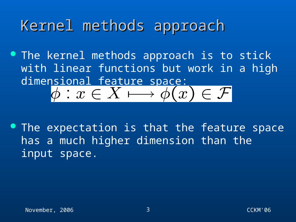
The kernel methods approach is to stick with linear functions but work in a high dimensional feature space:
The expectation is that the feature space has a much higher dimension than the input space.

November, 2006 CCKM'064
ExampleExample
Consider the mapping
If we consider a linear equation in this feature space:
We actually have an ellipse – i.e. a non-linear shape in the input space.
5
Capacity of feature spacesCapacity of feature spaces
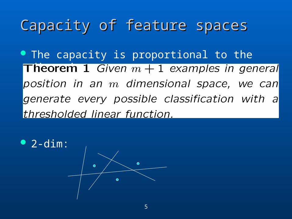
The capacity is proportional to the dimension
2-dim:

November, 2006 CCKM'066
Form of the functionsForm of the functions
So kernel methods use linear functions in a feature space:
For regression this could be the function For classification require thresholding

November, 2006 CCKM'067
Problems of high dimensionsProblems of high dimensions
Capacity may easily become too large and lead to over-fitting: being able to realise every classifier means unlikely to generalise well
Computational costs involved in dealing with large vectors
November, 2006 CCKM'068
RecallRecall
Two theoretical approaches converged on similar algorithms:1. Bayesian approach led to Bayesian inference using Gaussian
Processes2. Frequentist Approach: MLE
First we briefly discuss the Bayesian approach before mentioning some of the frequentist results
November, 2006 CCKM'069
I. I. Bayesian approachBayesian approach
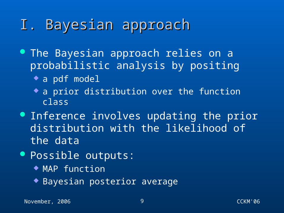
The Bayesian approach relies on a probabilistic analysis by positing a pdf model a prior distribution over the function class
Inference involves updating the prior distribution with the likelihood of the data
Possible outputs: MAP function Bayesian posterior average

November, 2006 CCKM'0610
Bayesian approachBayesian approach Avoids overfitting by
Controlling the prior distribution Averaging over the posterior
November, 2006 CCKM'0611
Bayesian approachBayesian approach
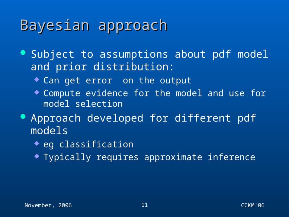
Subject to assumptions about pdf model and prior distribution: Can get error on the output Compute evidence for the model and use for model selection
Approach developed for different pdf models eg classification Typically requires approximate inference
November, 2006 CCKM'0612
2. 2. Frequentist approachFrequentist approach
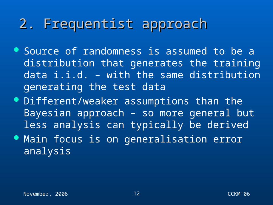
Source of randomness is assumed to be a distribution that generates the training data i.i.d. – with the same distribution generating the test data
Different/weaker assumptions than the Bayesian approach – so more general but less analysis can typically be derived
Main focus is on generalisation error analysis

November, 2006 CCKM'0613
GeneralizationGeneralization What do we mean by generalisation?

November, 2006 CCKM'0614
GeneraliGeneralizzation of a learneration of a learner

November, 2006 CCKM'0615
Example of GeneralisationExample of Generalisation
We consider the Breast Cancer dataset
Use the simple Parzen window classifier: weight vector is
where is the average of the positive (negative) training examples.
Threshold is set so hyperplane bisects the line joining these two points.
November, 2006 CCKM'0616
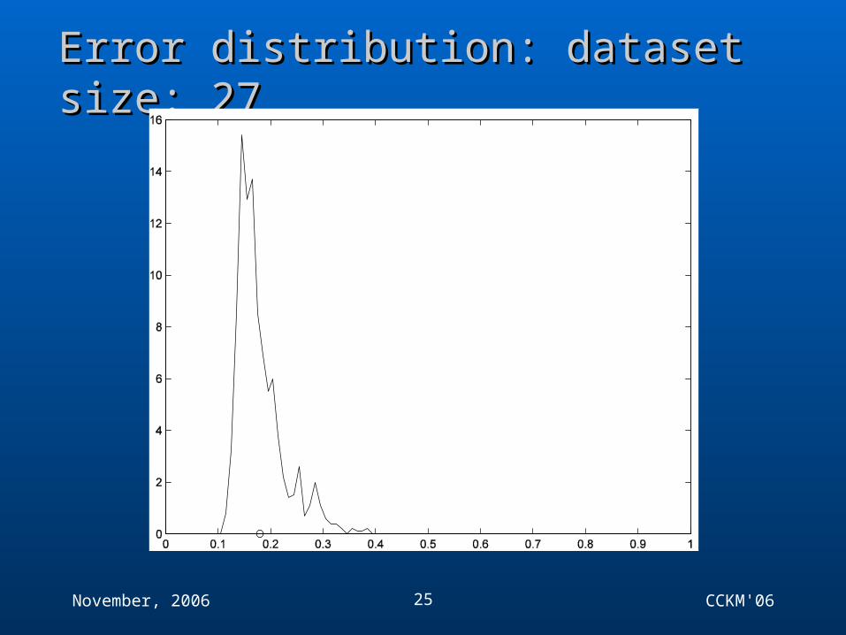
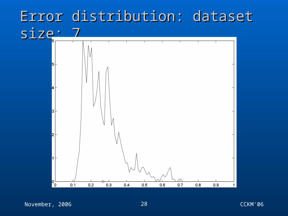
Example of GeneralisationExample of Generalisation
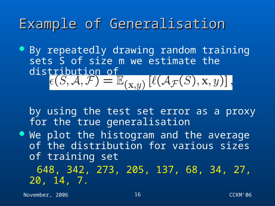
By repeatedly drawing random training sets S of size m we estimate the distribution of
by using the test set error as a proxy for the true generalisation
We plot the histogram and the average of the distribution for various sizes of training set
648, 342, 273, 205, 137, 68, 34, 27, 20, 14, 7.

November, 2006 CCKM'0617
Example of GeneralisationExample of Generalisation Since the expected classifier is in all cases the same
we do not expect large differences in the average of the distribution, though the non-linearity of the loss function means they won't be the same exactly.
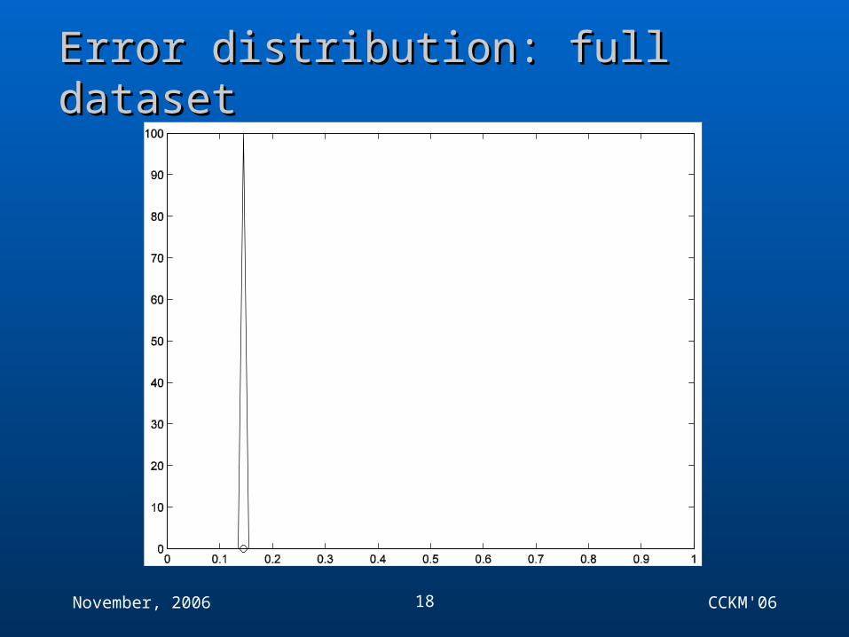
November, 2006 CCKM'0618
Error distribution: full datasetError distribution: full dataset

November, 2006 CCKM'0619
Error distribution: dataset size: 342Error distribution: dataset size: 342
November, 2006 CCKM'0620
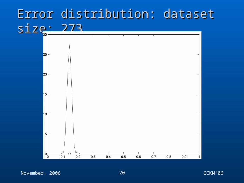
Error distribution: dataset size: 273Error distribution: dataset size: 273

November, 2006 CCKM'0621
Error distribution: dataset size: 205Error distribution: dataset size: 205

November, 2006 CCKM'0622
Error distribution: dataset size: 137Error distribution: dataset size: 137
November, 2006 CCKM'0623
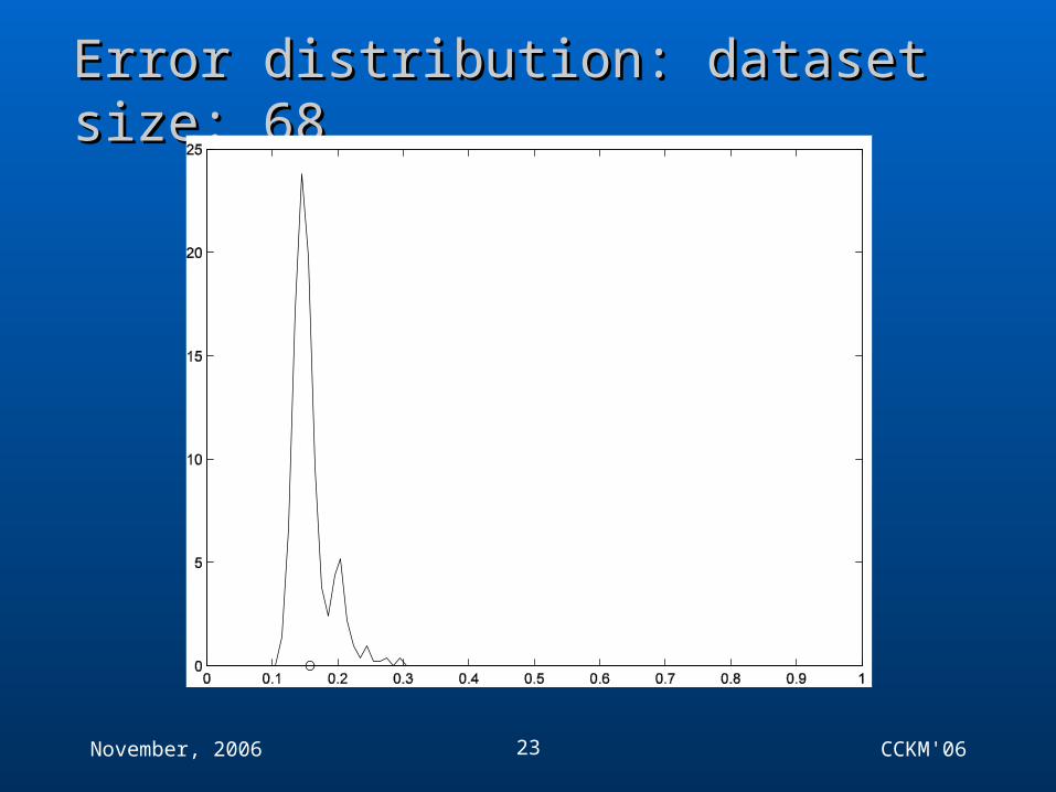
Error distribution: dataset size: 68Error distribution: dataset size: 68
November, 2006 CCKM'0624
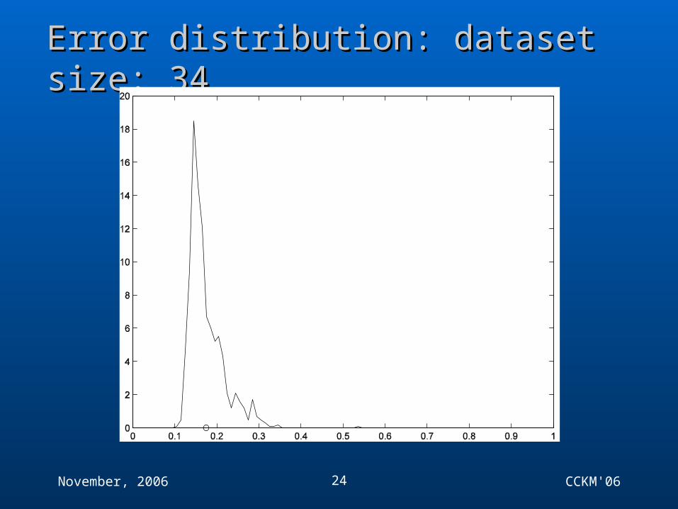
Error distribution: dataset size: 34Error distribution: dataset size: 34
November, 2006 CCKM'0625
Error distribution: dataset size: 27Error distribution: dataset size: 27

November, 2006 CCKM'0626
Error distribution: dataset size: 20Error distribution: dataset size: 20

November, 2006 CCKM'0627
Error distribution: dataset size: 14Error distribution: dataset size: 14
November, 2006 CCKM'0628
Error distribution: dataset size: 7Error distribution: dataset size: 7
November, 2006 CCKM'0629
ObservationsObservations
Things can get bad if number of training examples small compared to dimension Mean can be bad predictor of true generalisation – i.e. things can look okay in expectation, but still go badly
wrong Key ingredient of learning – keep flexibility high while still
ensuring good generalisation
November, 2006 CCKM'0630
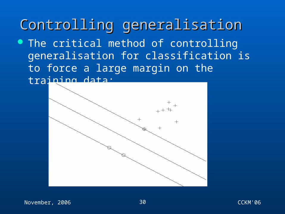
Controlling generalisationControlling generalisation The critical method of controlling generalisation for
classification is to force a large margin on the training data:
31
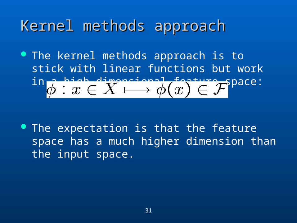
Kernel methods approachKernel methods approach
The kernel methods approach is to stick with linear functions but work in a high dimensional feature space:
The expectation is that the feature space has a much higher dimension than the input space.

Study: Hilbert Space Study: Hilbert Space
Functionals: A mapfrom vector space to a field Duality: Inner product Norm Similarity Distance Metric
32(C) 2006, SNU Biointelligence Lab, http://bi.snu.ac.kr/

Kernel FunctionsKernel Functions
k(x, x )=φ(x)Tφ(x ).For examplek(x, x )=(xTx’+c)M
What if x and x’ are two images? The kernel represents a particular weighted sum of all possible products of M pixels in the first image with M
pixels in the second image.
33

34
Kernel Function: Kernel Function: EEvaluated at the training data pointsvaluated at the training data points k(x, x’ )=k(x, x’ )=φ(φ(x)x)TTφ(φ(x’ ). x’ ). Linear Kernels: k;(x,x’) = xTx’
Stationary kernels: Invariant to translation
Homogeneous kernels, i.e., radial basis functions:
Kernel TrickKernel Trick
if we have an algorithm in which the input vector x enters only in the form of scalar products, then we can replace that scalar product with some other choice of kernel.
35
36
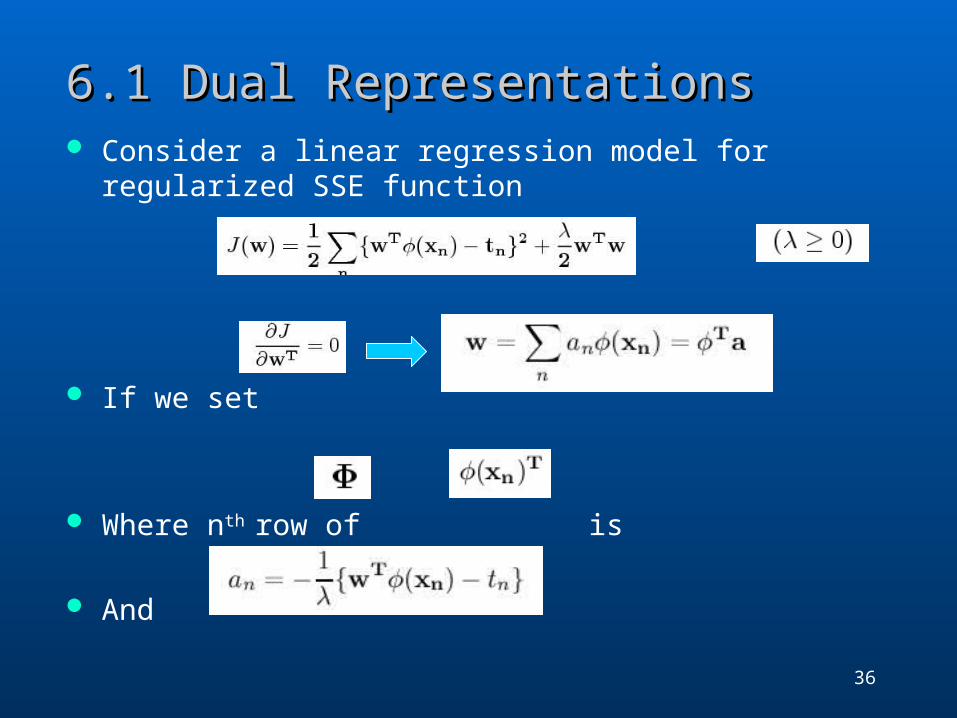
6.1 Dual Representations 6.1 Dual Representations Consider a linear regression model for regularized SSE function
If we set
Where nth row of is
And
37
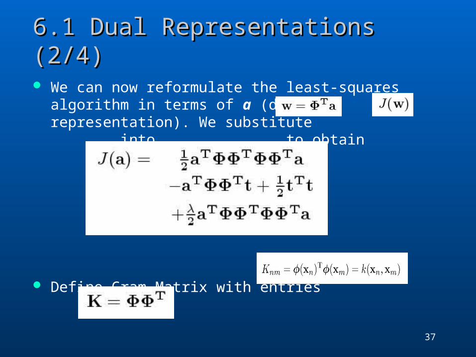
6.1 Dual Representations (2/4)6.1 Dual Representations (2/4)
We can now reformulate the least-squares algorithm in terms of a (dual representation). We substitute into to obtain
Define Gram Matrix with entries

38
6.1 Dual Representations (3/4)6.1 Dual Representations (3/4)
The sum-of-squares error function can be written as
Setting the gradient of with respect to a to zero, we obtain optimal a
Recall a was a function of w
39
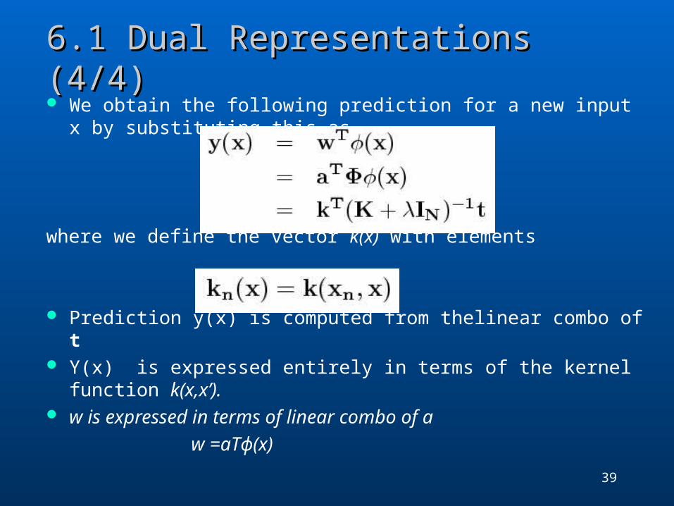
6.1 Dual Representations (4/4)6.1 Dual Representations (4/4) We obtain the following prediction for a new input x by substituting
this as
where we define the vector k(x) with elements
Prediction y(x) is computed from thelinear combo of t Y(x) is expressed entirely in terms of the kernel function k(x,x’). w is expressed in terms of linear combo of a w =aTф(x)
RecallRecall
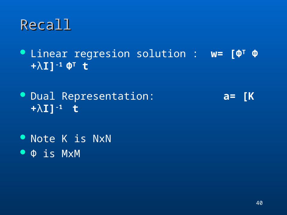
Linear regresion solution : w= [ΦT Φ +λI]-1 ΦT t
Dual Representation: a= [K +λI]-1 t
Note K is NxN Φ is MxM
40
41
6.2 Constructing Kernels (1/5)6.2 Constructing Kernels (1/5)
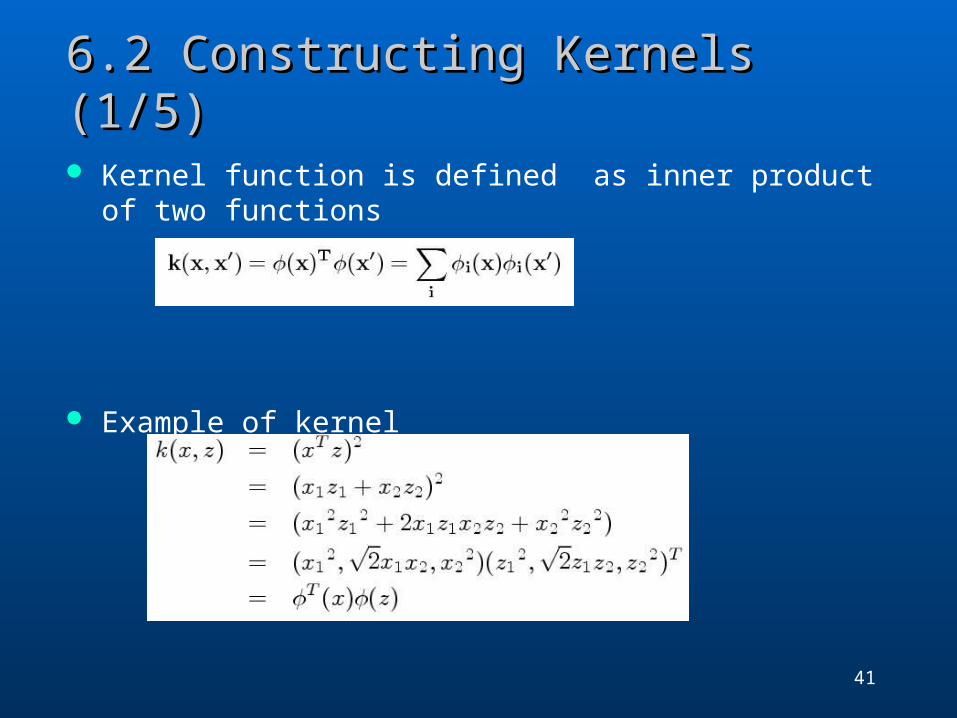
Kernel function is defined as inner product of two functions
Example of kernel
42(C) 2006, SNU Biointelligence Lab, http://bi.snu.ac.kr/
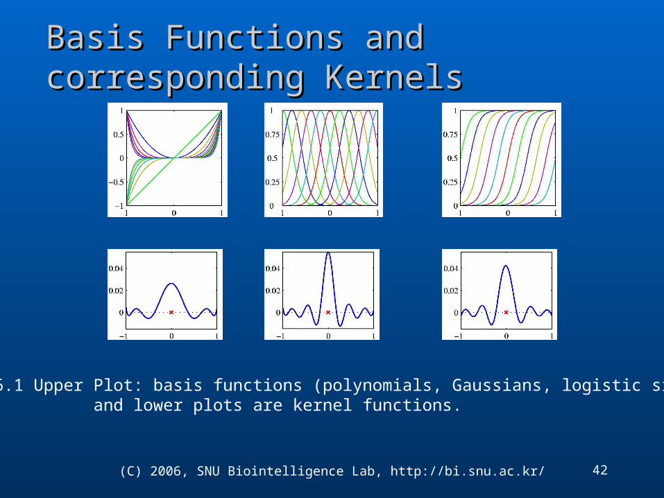
Basis Functions and corresponding KernelsBasis Functions and corresponding Kernels
Figure 6.1 Upper Plot: basis functions (polynomials, Gaussians, logistic sigmoid), and lower plots are kernel functions.
43(C) 2006, SNU Biointelligence Lab, http://bi.snu.ac.kr/
Constructing Kernels Constructing Kernels
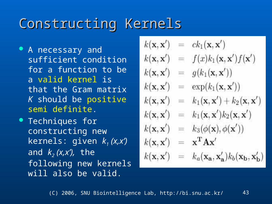
A necessary and sufficient condition for a function to be a valid kernel is that the Gram matrix K should be positive semi definite.
Techniques for constructing new kernels: given k1 (x,x’) and k2 (x,x’), the following new kernels will also be valid.

44(C) 2006, SNU Biointelligence Lab, http://bi.snu.ac.kr/
Gaussian KernelGaussian Kernel
Show that: The feature vector that corresponds to the Gaussian kernel has infinity dimensionality.

Construction of Kernels from Generative Construction of Kernels from Generative ModelsModels Given p(x), define a kernel function k((x,x’) = p(x)p(x’)
A kernel function measuring the similarity of two sequences: z is hidden variable
Leads to hidden Markov model if x and x’ are sequences of outcomes
45

Fisher KernelFisher Kernel
Consider Fisher Score: Then fisher kernel is defined as
Where F is the Fisher information matrix,
46(C) 2006, SNU Biointelligence Lab, http://bi.snu.ac.kr/

47
Sigmoid kernelSigmoid kernel
This sigmoid kernel form gives the support machine a superficial resemblance to neural network model.
48(C) 2006, SNU Biointelligence Lab, http://bi.snu.ac.kr/
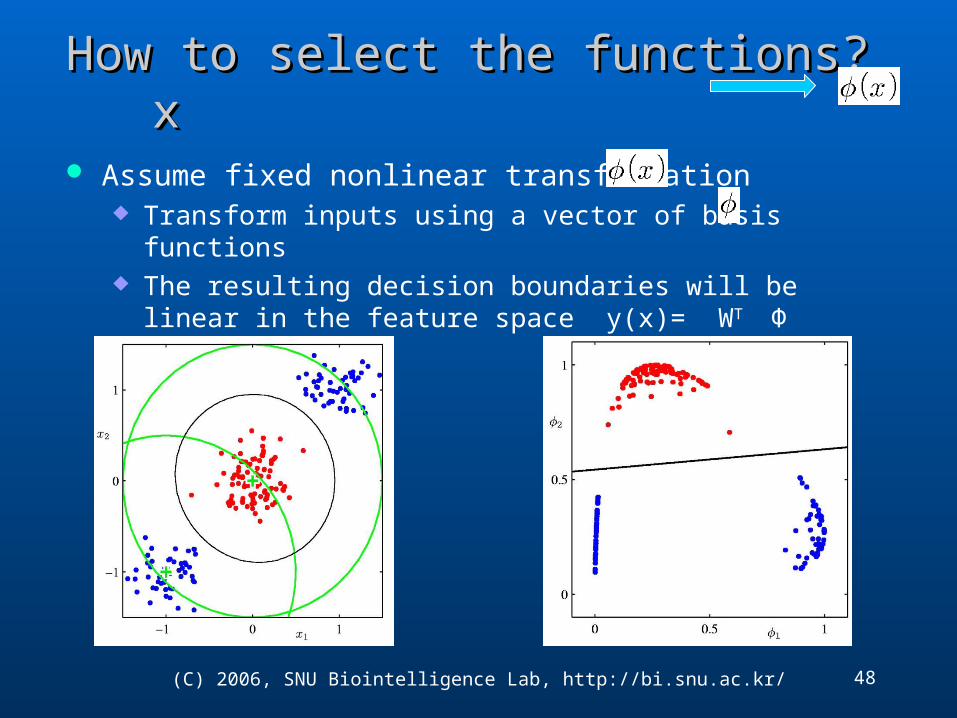
How to select theHow to select the functions functions? x ? x
Assume fixed nonlinear transformation Transform inputs using a vector of basis functions The resulting decision boundaries will be linear in the feature
space y(x)= WT Φ
49(C) 2006, SNU Biointelligence Lab, http://bi.snu.ac.kr/
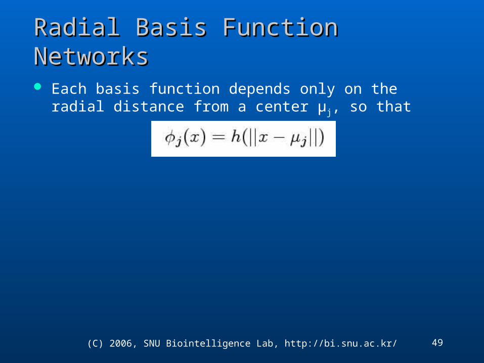
Radial Basis Function Networks Radial Basis Function Networks
Each basis function depends only on the radial distance from a center μj, so that

50(C) 2006, SNU Biointelligence Lab, http://bi.snu.ac.kr/
6.3 Radial Basis Function Networks (2/3)6.3 Radial Basis Function Networks (2/3)
Let’s consider of the interpolation problem when the input variables are noisy. If the noise on the input vector x is described by a variable ξ having a distribution ν(ξ), the sum-of-squares error function becomes as follows:
Using the calculus of variation,

51(C) 2006, SNU Biointelligence Lab, http://bi.snu.ac.kr/
6.3 Radial Basis Function Networks (3/3)6.3 Radial Basis Function Networks (3/3)
Figure 6.2 Gaussian basis functions and their normalized basis functions
52(C) 2006, SNU Biointelligence Lab, http://bi.snu.ac.kr/
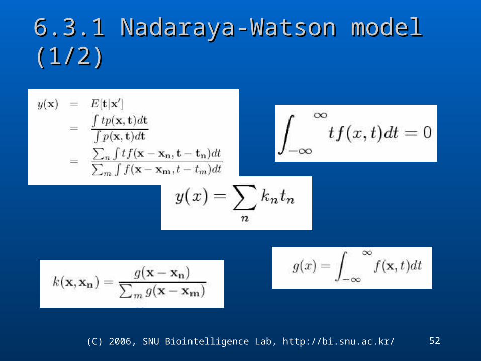
6.3.1 Nadaraya-Watson model (1/2)6.3.1 Nadaraya-Watson model (1/2)

53(C) 2006, SNU Biointelligence Lab, http://bi.snu.ac.kr/
6.3.1 Nadaraya-Watson model (2/2)6.3.1 Nadaraya-Watson model (2/2)
Figure 6.3 Illustration of the Nadaraya-Watson kernel regression model for sinusoid data set. The original sine function is the green curve. The data points are blue points and resulting regression line is red.
54(C) 2006, SNU Biointelligence Lab, http://bi.snu.ac.kr/
6.4 Gaussian Processes6.4 Gaussian Processes
We extend the role of kernels to probabilistic discriminative models.
We dispense with the parametric model and instead define a prior probability distribution over functions directly.
55(C) 2006, SNU Biointelligence Lab, http://bi.snu.ac.kr/
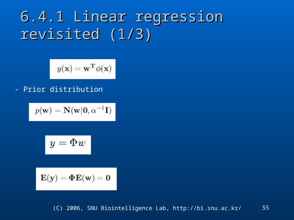
6.4.1 Linear regression revisited (1/3)6.4.1 Linear regression revisited (1/3)
- Prior distribution
56(C) 2006, SNU Biointelligence Lab, http://bi.snu.ac.kr/
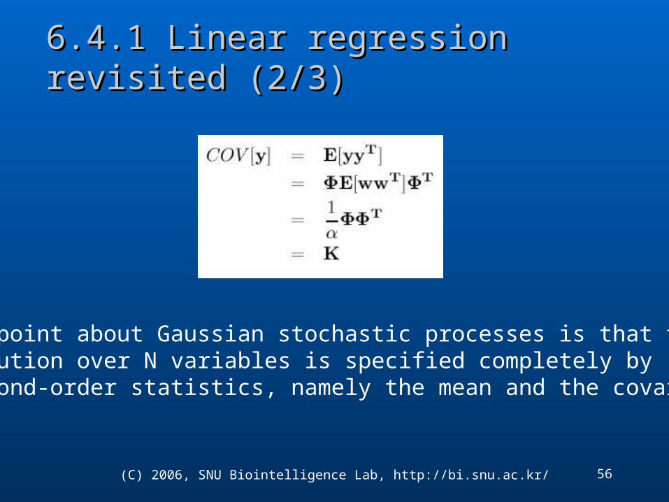
6.4.1 Linear regression revisited (2/3)6.4.1 Linear regression revisited (2/3)
-A key point about Gaussian stochastic processes is that the jointdistribution over N variables is specified completely by the second-order statistics, namely the mean and the covariance.

57(C) 2006, SNU Biointelligence Lab, http://bi.snu.ac.kr/
6.4.1 Linear regression revisited (3/3)6.4.1 Linear regression revisited (3/3)
Figure 6.4 Samples from Gaussian processes for a ‘Gaussian’ kernel (left)And an exponential kernel (right).
58(C) 2006, SNU Biointelligence Lab, http://bi.snu.ac.kr/
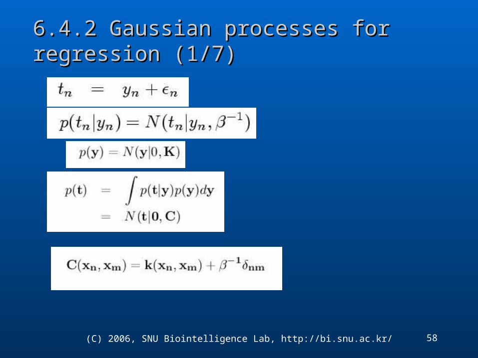
6.4.2 Gaussian processes for regression (1/7)6.4.2 Gaussian processes for regression (1/7)

59(C) 2006, SNU Biointelligence Lab, http://bi.snu.ac.kr/
6.4.2 Gaussian processes for regression (2/7)6.4.2 Gaussian processes for regression (2/7)
One widely used kernel function for Gaussian process regression
Figure 6.5 Samples from aGaussian process priorDefined by theabove covariance function.
60(C) 2006, SNU Biointelligence Lab, http://bi.snu.ac.kr/
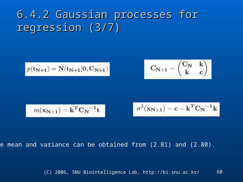
6.4.2 Gaussian processes for regression (3/7)6.4.2 Gaussian processes for regression (3/7)
Above mean and variance can be obtained from (2.81) and (2.80).
61(C) 2006, SNU Biointelligence Lab, http://bi.snu.ac.kr/
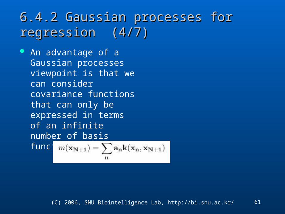
6.4.2 Gaussian processes for regression (4/7)6.4.2 Gaussian processes for regression (4/7)
An advantage of a Gaussian processes viewpoint is that we can consider covariance functions that can only be expressed in terms of an infinite number of basis functions.

62(C) 2006, SNU Biointelligence Lab, http://bi.snu.ac.kr/
6.4.2 Gaussian processes for regression (5/7)6.4.2 Gaussian processes for regression (5/7)
Figure 6.6 Illustration of the sampling of data points {tn} from a Gaussian process.The blue curve shows a sample function and the red points show the value of yn.The corresponding values of {tn}, shown in green, are obtained by adding independentGaussian noise to each of the {yn}.

63
6.4.2 Gaussian processes for regression (6/7)6.4.2 Gaussian processes for regression (6/7)
Gaussian process regression for the case of one training point and one test point, in which the red ellipses show contours of the joint dis-tribution p(t1 ,t2). t1 is the training data point, and conditioningon thevalueof t1 , corresponding to the vertical blue line, we obtain p(t2|t1) shown as a function of t2 by the green curve.

64(C) 2006, SNU Biointelligence Lab, http://bi.snu.ac.kr/
6.4.2 Gaussian processes for regression (8/7)6.4.2 Gaussian processes for regression (8/7)
Figure 6.8 Illustration of Gaussian process regression applied to the sinusoidal data set.The green curve shows the sinusoidal function from which the data points, shown in blue,are obtained by sampling and addition of Gaussian noise. The red line shows the mean ofthe Gaussian process predictive distribution.
65(C) 2006, SNU Biointelligence Lab, http://bi.snu.ac.kr/
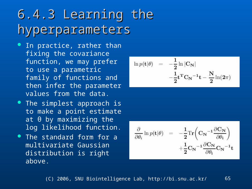
6.4.3 Learning the hyperparameters6.4.3 Learning the hyperparameters
In practice, rather than fixing the covariance function, we may prefer to use a parametric family of functions and then infer the parameter values from the data.
The simplest approach is to make a point estimate at θ by maximizing the log likelihood function.
The standard form for a multivariate Gaussian distribution is right above.
66(C) 2006, SNU Biointelligence Lab, http://bi.snu.ac.kr/
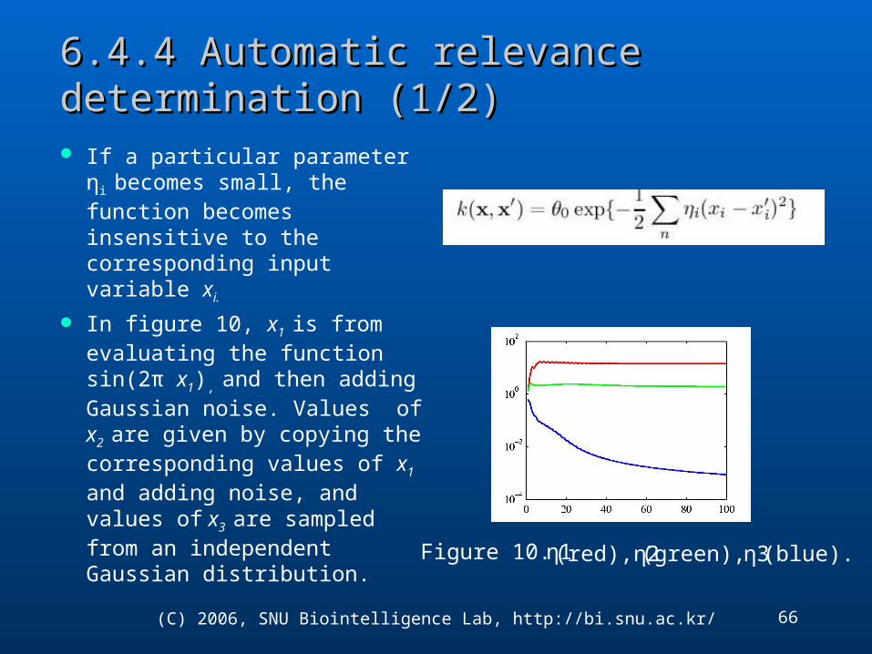
6.4.4 Automatic relevance determination (1/2)6.4.4 Automatic relevance determination (1/2)
If a particular parameter ηi
becomes small, the function becomes insensitive to the corresponding input variable xi.
In figure 10, x1 is from evaluating the function sin(2π x1), and then adding Gaussian noise. Values of x2 are given by copying the corresponding values of x1 and adding noise, and values of x3 are sampled from an independent Gaussian distribution.
Figure 10. η1 (red), η2 (green), η3 (blue).
67(C) 2006, SNU Biointelligence Lab, http://bi.snu.ac.kr/
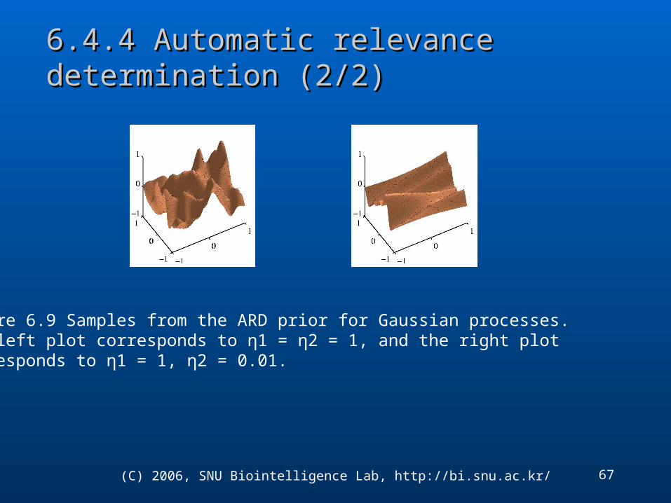
6.4.4 Automatic relevance determination (2/2)6.4.4 Automatic relevance determination (2/2)
Figure 6.9 Samples from the ARD prior for Gaussian processes. The left plot corresponds to η1 = η2 = 1, and the right plot Corresponds to η1 = 1, η2 = 0.01.

68(C) 2006, SNU Biointelligence Lab, http://bi.snu.ac.kr/
6.4.5 Gaussian processes for classification (1/2)6.4.5 Gaussian processes for classification (1/2)
aN+1 is the independent variable of logistic function.
-One technique is based on variational inference. This approach
yields a lower bound on the likelihood function.
- The second approach uses expectation propagation.

69(C) 2006, SNU Biointelligence Lab, http://bi.snu.ac.kr/
6.4.5 Gaussian processes for classification (2/2)6.4.5 Gaussian processes for classification (2/2)
Figure 6.11 The left plot shows a sample from a Gaussian processprior over functions a(x), and right plot shows the result of Transforming this sample using a logistic sigmoid function.

70(C) 2006, SNU Biointelligence Lab, http://bi.snu.ac.kr/
6.4.6 Laplace approximation (1/8)6.4.6 Laplace approximation (1/8)
The third approach to Gaussian process classification is based on the Laplace approximation.

71(C) 2006, SNU Biointelligence Lab, http://bi.snu.ac.kr/
6.4.6 Laplace approximation (2/8)6.4.6 Laplace approximation (2/8)
We then obtain the Laplace approximation by Taylor expanding the logarithm of P(aN|tN), which up to an additive normalization constant is given by the quantity
We resort to the iterative scheme based on the Newton-Raphson method, which gives rise to an iterative reweighted least squares (IRLS) algorithm.

72(C) 2006, SNU Biointelligence Lab, http://bi.snu.ac.kr/
6.4.6 Laplace approximation (3/8)6.4.6 Laplace approximation (3/8)
- Where WN is a diagonal matrix elements .
-Using the Newton-Raphson formula, the iterative update equation for aN is given by
73(C) 2006, SNU Biointelligence Lab, http://bi.snu.ac.kr/
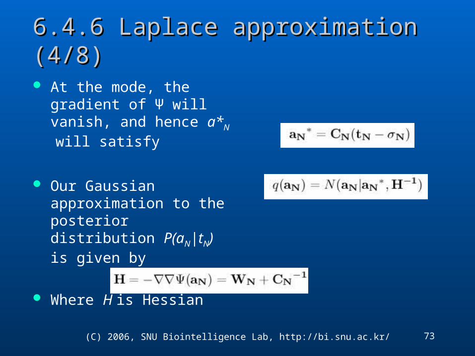
6.4.6 Laplace approximation (4/8)6.4.6 Laplace approximation (4/8)
At the mode, the gradient of Ψ will vanish, and hence a*N
will satisfy
Our Gaussian approximation to the posterior distribution P(aN|tN) is given by
Where H is Hessian
74(C) 2006, SNU Biointelligence Lab, http://bi.snu.ac.kr/
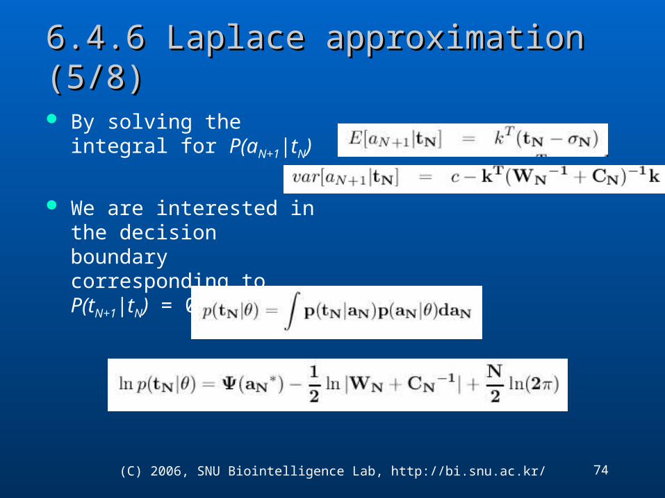
6.4.6 Laplace approximation (5/8)6.4.6 Laplace approximation (5/8)
By solving the integral for P(aN+1|tN)
We are interested in the decision boundary corresponding to P(tN+1|tN) = 0.5

75(C) 2006, SNU Biointelligence Lab, http://bi.snu.ac.kr/
6.4.6 Laplace approximation (6/8)6.4.6 Laplace approximation (6/8)
76(C) 2006, SNU Biointelligence Lab, http://bi.snu.ac.kr/
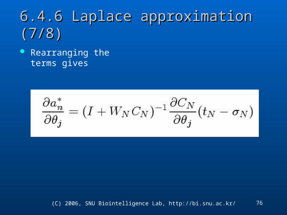
6.4.6 Laplace approximation (7/8)6.4.6 Laplace approximation (7/8)
Rearranging the terms gives

77(C) 2006, SNU Biointelligence Lab, http://bi.snu.ac.kr/
6.4.6 Laplace approximation (8/8)6.4.6 Laplace approximation (8/8)
Figure 6.12 Illustration of the use of a Gaussian proccess forClassification. The true distribution is green, and the decisionBoundary from the Gaussian process is black. On the rightis the predicted posterior probability for the blue and red classestogether with the Gaussian process decision boundary.
78(C) 2006, SNU Biointelligence Lab, http://bi.snu.ac.kr/
6.4.7 Connection to neural networks6.4.7 Connection to neural networks
Neal has shown that, for a broad class of prior distributions over w, the distribution of functions generated by a neural network will tend to a Gaussian process in the linit M->00, where M is the number of hidden units.
By working directly with the covariance function we have implicitly marginalized over the distribution of weights. If the weight prior is governed by hyperparameters, then their values will determine the length of scales of the distribution over functions. Note that we cannot marginalize out the hyperparameters analytically, and must instead resort to techniques of the kind discussed in Section 6.4.