recent progress in analytical solutions of the boussinesq ... · recent progress in analytical...

Recent progress in analytical solutions of theBoussinesq nonlinear groundwater equation

3rd Brazilian Soil Physics Meeting, May 4th 2015

Nelson Luís Dias1

1Professor, Department of Environmental Engineering, Universidade Federal do Paraná,e-mail: [email protected]. url: www.lemma.ufpr.br/nldias

May 04 2015

LemmaUFPR

[email protected]

www.lemma.ufpr.br/nldias

Summary 1/34

Summary

1. Thanks2. Introduction3. The Boussinesq ODE, and its cousin the Blasius ODE4. The search for solutions5. Solutions for ϕ0 = 06. Solutions for ϕ0 , 07. An application to hydrology8. Conclusions

LemmaUFPR

1. Thanks 2/34

Thanks and acknowledgements

It is an honor to be here, to speak to you.

Thanks to the organizing commi�ee, in particular to Robson Armindo, for the invitation.

This talk is largely based on Tomás Chor’s MSc thesis and joint publications with TomásChor and Ailín Ruiz de Zárate.

LemmaUFPR

2. Introduction 3/34

2. Introduction

The Boussinesq nonlinear PDE for groundwater (for a horizontal acquifer) was derivedby Boussinesq in 1903. Its assumptions are

• conservation of mass

• Darcy’s law

• horizontal mean velocity (Dupuit-Forchheimer)

The 1-D version of the equation, for a horizontal aquifer, is

∂h

∂t=k

n

∂

∂x

[h∂h

∂x

].

• k is the saturated hydraulic conductivity,• n is the drainable porosity.

LemmaUFPR


Meet Boussinesq

LemmaUFPR


Why is it important?

The equation, although it involves some approximations, is a very good model forthe drought flow of an aquifer into free-surface streams, such as rivers and drainagetrenches.

b

b

L

H0

H

BB

x

h(x, t)

LemmaUFPR


Why is it important?

• As such, it can predict the outflow from an aquifer accurately [Ibrahim and Brutsaert,1965], as well as predict the free surface when B/H > 4 [Verma and Brutsaert, 1971,p. 1227]

• Various solutions of the Boussinesq equation can be used together to solve an “inverseproblem”: from the outflow hydrograph, obtain the physical and geometrical param-eters of the aquifer (usually, two among: k , n, B, H ). This is called “Brutsaert-Nieber”recession analysis, from its seminal paper [Brutsaert and Nieber, 1977].

• Recent uses of this equation include the linking of geological and geomorphologicalfeatures to hydrological behavior [Mutzner et al., 2013, Vannier et al., 2014] and thedefinition of good engineering practices for the robust calibration of parsimoniousmodels [Melsen et al., 2014].

LemmaUFPR


Focus

• As usual, there is a very large field of themes to investigate regarding the Boussinesqnon-linear PDE.

• In this talk, I will concentrate on the particular case B → ∞. The PDE can then besimplified to an ODE.

• It is this ODE, and a sequence of proposed solutions, that we will be talking abouthere.

LemmaUFPR


Focus

• As usual, there is a very large field of themes to investigate regarding the Boussinesqnon-linear PDE.

• In this talk, I will concentrate on the particular case B → ∞. The PDE can then besimplified to an ODE.

• It is this ODE, and a sequence of proposed solutions, that we will be talking abouthere.

Unfortunately, whenever we have focus on a problem, di�iculties mount.

We end up spending a lot of energy on the focused problem, which is but a small part ofthe problem we started with.

Please, bear with us as we probe the many facets and di�iculties of some solutions of theBoussinesq ODE!

LemmaUFPR

3. The Boussinesq ODE, and its cousin the Blasius ODE 8/34

3. The Boussinesq ODE, and its cousin the Blasius ODE

LemmaUFPR



We are interested in the case B → ∞.Given a Boltzmann transformation,

ϕ =h(x ,t )

H, ξ =

x√4Dt, D = H

k

n,

the Boussinesq PDE is transformed into

ddξ

(ϕdϕdξ

)+ 2ξ dϕdξ = 0.

LemmaUFPR




ϕ =h(x ,t )

H, ξ =

x√4Dt, D = H

k

n,


ddξ

(ϕdϕdξ

)+ 2ξ dϕdξ = 0.

Surprisingly, Punnis [1956] showed that,if we further put

ϕ =dfdη , ξ =

12 f ,

we obtain

d3 fdη3+12 f

d2 fdη2= 0,

which is Blasius’ equation for a laminarboundary-layer!

LemmaUFPR




ϕ =h(x ,t )

H, ξ =

x√4Dt, D = H

k

n,


ddξ

(ϕdϕdξ

)+ 2ξ dϕdξ = 0.

Surprisingly, Punnis [1956] showed that,if we further put

ϕ =dfdη , ξ =

12 f ,

we obtain

d3 fdη3+12 f

d2 fdη2= 0,

which is Blasius’ equation for a laminarboundary-layer!

This means that in principle we can apply everything we know about Blasius’ solutionof f to Boussinesq’s solution of ϕ. We will call this the Punnis transformation.

LemmaUFPR


The legacy of Blasius

There is a lot to be learned from Blasius [1908]’s Boundary-Layer Theory. Remember,Blasius’s advisor was Ludwig Prandtl, the creator of the Boundary-Layer concept.

Ludwig Prandtl (le�) and Paul Richard Heinrich Blasius (right).

LemmaUFPR


In 1950, NACA (nowadays NASA) was interested in Blasius [1908].

LemmaUFPR


In 1950, NACA (nowadays NASA) was interested in Blasius [1908].

Blasius’ did not stop at deriving his equa-tion. The main tools he used were:

• The product of two series is again a se-ries

• A solution for f in series can be de-veloped, but the radius of convergencearound η = 0 is finite.

• Beyond the radius of convergence, Bla-sius implemented an asymptotic solu-tion.

LemmaUFPR


Blasius’ essential mathematical tools

Series products

∞∑n=0

Anxn

∞∑m=0

Bmxm

=

∞∑n=0

n∑m=0

AmBn−mxn.

This allows us to seek series solutions of non-linear di�erential equations. Finding theradius of convergence of these solutions, however, can be quite di�icult.

Asymptotic behaviorMoreover, we may try to modify the ODE by “knowing” some asymptotic behavior. Inour case, if we start out from an aquifer full of water up to H at t = 0, and if B = ∞, weexpect

limξ→∞

ϕ (ξ ) = 1.

Substituting back this condition or a zero derivative in the Boussinesq ODE may resultin a simpler ODE, valid for large ξ only.

LemmaUFPR

4. The search for solutions 12/34

4. The search for solutions

LemmaUFPR



In order for the Boltzmann transform to work, weneed to collapse two Boundary Conditions intoone:

ϕ =h(x ,t )

H, ξ =

x√4Dt, D = H

k

n,

h(x ,0) = H

h(∞,t ) = H⇒ ϕ (∞) = 1,

h(0,t ) = H0 ⇒ ϕ (0) = ϕ0.

This is a boundary-value problem. Physically,however, we are interested in the initial condition

ψ0 = ϕdϕdξ

��ξ=0,

which gives the flow rate out of the aquifer andinto the stream.

LemmaUFPR



In order for the Boltzmann transform to work, weneed to collapse two Boundary Conditions intoone:

ϕ =h(x ,t )

H, ξ =

x√4Dt, D = H

k

n,

h(x ,0) = H

h(∞,t ) = H⇒ ϕ (∞) = 1,

h(0,t ) = H0 ⇒ ϕ (0) = ϕ0.

This is a boundary-value problem. Physically,however, we are interested in the initial condition

ψ0 = ϕdϕdξ

��ξ=0,

which gives the flow rate out of the aquifer andinto the stream.

• The shooting method consists of guessingψ0, solving numerically the Boussinesq ODE,checking ϕ (∞) (where “∞” is just a largeenough ξ ), adjusting ψ0, and going over (untilϕ (∞) ≈ 1).

• Töpfer’s (1912) method,

ϕ = λ−2ϕ∗, ψ = λ−3ψ ∗, ξ = λ−1ξ ∗,

avoids the iterations, but only when ϕ0 = 0.

• No ma�er what the subsequent analytical ap-proach is, a numerical solution (e.g. Runge-Ku�a) is needed to obtainψ0.

LemmaUFPR

5. Solutions for ϕ0 = 0 13/34

5. Solutions for ϕ0 = 0

Given the Blasius equation, with boundary conditions f (0) = 0, f ′(0) = 0, f ′(∞) = 1,Blasius derived

f (η) =∞∑n=0

(−1)nanη3n+2, an =1

2(3n + 2) (3n + 1) (3n)

n−1∑k=0

(3k + 2) (3k + 1)akan−1−k ,

where a0 = κ/2 and f ′′(0) = κ = 0.33205733621519630 [Boyd, 2008].

LemmaUFPR


5. Solutions for ϕ0 = 0

Given the Blasius equation, with boundary conditions f (0) = 0, f ′(0) = 0, f ′(∞) = 1,Blasius derived

f (η) =∞∑n=0

(−1)nanη3n+2, an =1

2(3n + 2) (3n + 1) (3n)

n−1∑k=0

(3k + 2) (3k + 1)akan−1−k ,

where a0 = κ/2 and f ′′(0) = κ = 0.33205733621519630 [Boyd, 2008].

Using the Punnis transformation, both Heaslet and Alksne [1961] and Polubarinova-Kochina [1962] inverted the Blasius series and obtained a few terms of a series solutionfor the Boussinesq EDO; they also obtained from Blasius an asymptotic solution:

ϕ (ξ ) = 1.152ξ 1/2 − 415ξ

2 + 0.0462ξ 7/2 − 0.00065ξ 5 + . . . ,ϕ (ξ ) ≈ 1 − 0.231√π erfc(ξ ).

LemmaUFPR


Heaslet and Alksne [1961]’s results were already very good

0.0

0.2

0.4

0.6

0.8

1.0

1.2

0 1 2 3 4 5

ϕ

ξ

numericalHeaslet & Alksne, series

Heaslet & Alksne, asymptotic

LemmaUFPR


Improvements: Hogarth and Parlange [1999]

The next step was provided by Hogarth and Parlange [1999]: they replaced the Heaslet&Alksne–Polubarinova-Kochina series solution with a Padé approximation obtained fromthat series, and also improved the asymptotic solution:

ϕ (ξ ) = 1.15249ξ 1/2 − 4/15ξ 2

1 + 0.17355ξ 3/2 + 0.02768ξ 3, ξ ≤ 1.3,

ϕ (ξ ) = 1 − 0.41387 erfc(

ξ

1 + 0.058375ξ 3 exp(−ξ 2)), ξ > 1.3.

LemmaUFPR


Improvements: Hogarth and Parlange [1999]

The next step was provided by Hogarth and Parlange [1999]: they replaced the Heaslet&Alksne–Polubarinova-Kochina series solution with a Padé approximation obtained fromthat series, and also improved the asymptotic solution:

ϕ (ξ ) = 1.15249ξ 1/2 − 4/15ξ 2

1 + 0.17355ξ 3/2 + 0.02768ξ 3, ξ ≤ 1.3,

ϕ (ξ ) = 1 − 0.41387 erfc(

ξ

1 + 0.058375ξ 3 exp(−ξ 2)), ξ > 1.3.

So far, everything was being obtained on the basis of Blasius’ results alone!

LemmaUFPR


Hogarth and Parlange [1999]’s results were more accurate

(but visually not too di�erent)

0.0

0.2

0.4

0.6

0.8

1.0

1.2

0 1 2 3 4 5

ϕ

ξ

numericalHogarth& Parlange, Padé

Hogarth& Parlange, asymptotic

LemmaUFPR


Direct series solution of the Boussinesq ODE

We approached the problem again in Tomás Chor’s MSc thesis, but we searched directlyfor a series solution of the Boussinesq ODE:

ϕ (ξ ) =∞∑n=0

anξ(3n+1)/2.

We first used symbolic algebra to compute the first n values of the series:1 M : 50 ;2 a[0]: 1.15248832742929 ;3 fi : sum(a[n]*x^((3*n+1)/2) ,n,0,M) ;4 eq : expand( diff(fi*diff(fi ,x),x) + 2*x*diff(fi ,x) ) ;5 cond : [] ;6 file_output_append : true ;7 with_stdout (" se_xi.txt",print(string(float(a [0]))));8 for n : 0 thru M-1 do (9 eqqu : ev(coeff(eq ,x ,(3*n+1)/2) , cond) ,10 this : solve(eqqu ,a[n+1]) ,11 cond : append(cond ,this),12 this : first(this),13 a[n+1] : rhs(this),14 with_stdout (" se_xi.txt",print(float(a[n+1])))15 );

LemmaUFPR


Results with symbolic algebra

We can go as far as we want with the an’s:

a0 +1,15248832742929 × 10+0a1 −2,6666666666667 × 10−1a2 +4,6276679827463 × 10+0a3 −6,4894881692528425 × 10−4a4 −9,4517828664332276 × 10−4a5 −2,5400784492116708 × 10−5a6 +3,5810599703874529 × 10−5a7 +3,8844564686017651 × 10−6a8 −1,4163383082670557 × 10−6a9 −3,2740710683167304 × 10−7a10 +4,5534502970990704 × 10−8 From Chor et al. [2013b]

LemmaUFPR


With hard algebra

Next, results were derived analytically [Chor et al., 2013a]:

an+1 = − 1a0(3n + 5)

*.,

4 (3n + 1) an3n + 3 +

3n + 52

n∑k=1

akan−k+1+/-,

a0√2ψ0

a1 − 415

a2 − 16a0 (2a1 + 3a

21)

a3 − (99a1+28)a299a0

a4 − (42a1+10)a3+21a2242a0... ...

Some limitations are inherited from theBlasius’ series solution:

• No equation for the general term (a rec-curence relation instead): no easy wayto calculate the radius of convergence.

• Dependence on the first term. In ourcase,

ψ0 = ϕdϕdξ

��ξ=0is a key parameter.

LemmaUFPR


Still, the radius of convergence was not known

Series solution calculated with 8700terms:

0.0

0.2

0.4

0.6

0.8

1.0

1.2

0.0 0.5 1.0 1.5 2.0 2.5

ϕ(ξ)

ξ

To obtain an accurate estimate of the ra-dius of convergence, we changed variables(ζ = ξ 1/2), obtained a new equation,

ddζ

[Φ

ζ

dΦdζ

]+ 4ζ 2dΦdζ = 0,

and a standard power series

Φ =∞∑n=0

anζ3n+1.

Φ(ζ ) is an analytic function within a circle around the origin in the complex ζ -plane.The circle’s radius is the radius of convergence. Within that radius, from Cauchy’s The-orem, ∮

CΦ(ζ ) dζ = 0.

LemmaUFPR


The radius of convergence

R ≈ 2.3757445

Re ζ

Im ζ

θ

θ

A B B′

b

All integrals are line integrals using the Runge-Ku�a-Cash-Karp method in the complexplane. The method provides error estimates which are used to identify non-zero lineintegrals. Six singularities of the complex Boussinesq function Φ(ζ ) are clearly seen,along with branch cuts emanating from them.

LemmaUFPR


Chor et al. [2013a] improvements

Having the full series now, we extended the Padé approximations

PN (ξ ) = ξ1/2

∑Nn=0Anξ

3n2∑N

n=0 Bnξ3n2.

Best results were obtained for N = 200, and a more modest N = 20 was tabulated. WithN = 20, the Padé approximation extends the radius of convergence to ≈ 3.3.

The same asymptotic solution of Hogarth and Parlange [1999],

ϕ (ξ ) ∼ 1 −A√π erfc *.,

ξ

1 + A2ξ 3 exp(−ξ 2)

+/-

was also obtained, but with A = 0.2337276186438419.

LemmaUFPR


Best results (But probably overkill)

0.0

0.2

0.4

0.6

0.8

1.0

1.2

1.4

0.0 1.0 2.0 3.0 4.0 5.0 6.0ξ

PadéAsymptotic

LemmaUFPR

6. Solutions for ϕ0 , 0 24/34

6. Solutions for ϕ0 , 0

We now look at the boundary condition 0 < ϕ0 < 1. As before, ϕ (∞) = 1.

Di�erently from the case ϕ0 = 0, the derivative dϕ/dξ is not singular at ξ = 0, and thisallows one to seek a solution in terms of a regular Taylor series [Dias et al., 2014]:

ϕ (ξ ) =∞∑n=0

anξn,

a0 = ϕ0, a1 =ψ0a0,

an+1 = − 1a0(n + 1)

2(n − 1)n

an−1 +n∑

k=1(n − k + 1)akan−k+1

.

LemmaUFPR


A practical approach for the initial condition

As before, the value of ψ0 is of engineering interest, but cannot be obtained (so far) bypurely analytical means. Töpfer’s method can no longer be applied to obtainψ0 (numer-ically) in one pass, but it can help to generate a large number of numerical solutions [seeDias et al., 2014]. Then, we fi�ed an empirical curve:

0.0

0.1

0.2

0.3

0.4

0.5

0.6

0.7

0.0 0.2 0.4 0.6 0.8 1.0

ψ0

ϕ0

Data pointsEq. (14)

ψ0(ϕ0) ≈ (Ψd0 + aϕ

b0)

1d (1 − ϕc0) (1 + f ϕ

д0)e ,

Ψ0 ≈ 0.66411467.

with a = 0.733841, b = 0.999223, c =0.98359, d = 2.94568, e = 0.186587, f =0.966673, and д = 0.93347.

LemmaUFPR


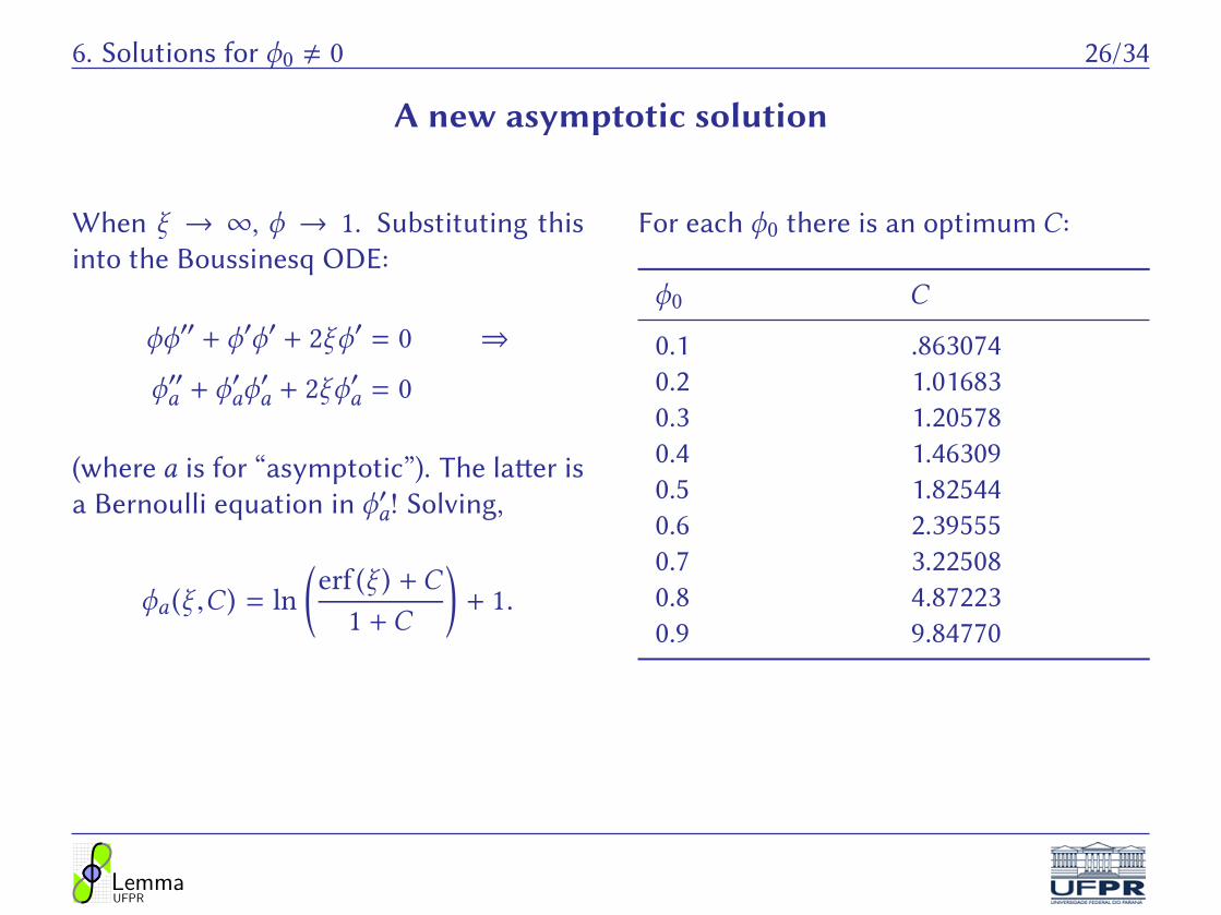
A new asymptotic solution

When ξ → ∞, ϕ → 1. Substituting thisinto the Boussinesq ODE:

ϕϕ′′ + ϕ′ϕ′ + 2ξϕ′ = 0 ⇒ϕ′′a + ϕ′aϕ′a + 2ξϕ′a = 0

(where a is for “asymptotic”). The la�er isa Bernoulli equation in ϕ′a! Solving,

ϕa (ξ ,C ) = ln(erf (ξ ) +C1 +C

)+ 1.

For each ϕ0 there is an optimum C :

ϕ0 C

0.1 .8630740.2 1.016830.3 1.205780.4 1.463090.5 1.825440.6 2.395550.7 3.225080.8 4.872230.9 9.84770

LemmaUFPR


Results from Dias et al. [2014] for ϕ0 = 0.5

0.0

0.2

0.4

0.6

0.8

1.0

1.2

0.0 0.5 1.0 1.5 2.0 2.5 3.0

ϕ(ξ)

ξ

NumericalAsymptotic

Padé

LemmaUFPR

7. An application to hydrology 28/34

7. An application to hydrology

Consider again a simplified watershed:

b

b

L

H0

H

BB

x

h(x, t)

In the dimensionless variables

x =x

B, τ =

kH

nB2t ,

the Boussinesq PDE is

∂ϕ

∂τ=∂

∂x

[ϕ∂ϕ

∂x

],

ϕ (x,0) = 1, ϕ (0,t ) = ϕ0,∂ϕ

∂x(1,t ) = 0.

At an early time the aquifer “looks” infinite alongx, and the dimensionless outflow is

χ (τ ) =

[ϕ∂ϕ

∂x

](0,τ ) =

[ϕdϕdξ

]

0

12τ−1/2 =

ψ02 τ−1/2.

For late times, a linearized equation can be derived[Boussinesq, 1904],

∂ϕ

∂τ= p∂2ϕ

∂x2

whose solution reduces to

χ (τ ) = p exp(−π2p

4 τ

).

Hence,dχdτ = α χ

β

LemmaUFPR


Brutsaert-Nieber recession analysis

α1 and α2 are analytically related to k and n. β1 = 3 and β2 = 1 are predicted from theanalytical solutions.

0.0001

0.001

0.01

0.1

1

10

100

1000

10000

0.01 0.1 1 10

|dχ/dτ|

χ

LemmaUFPR


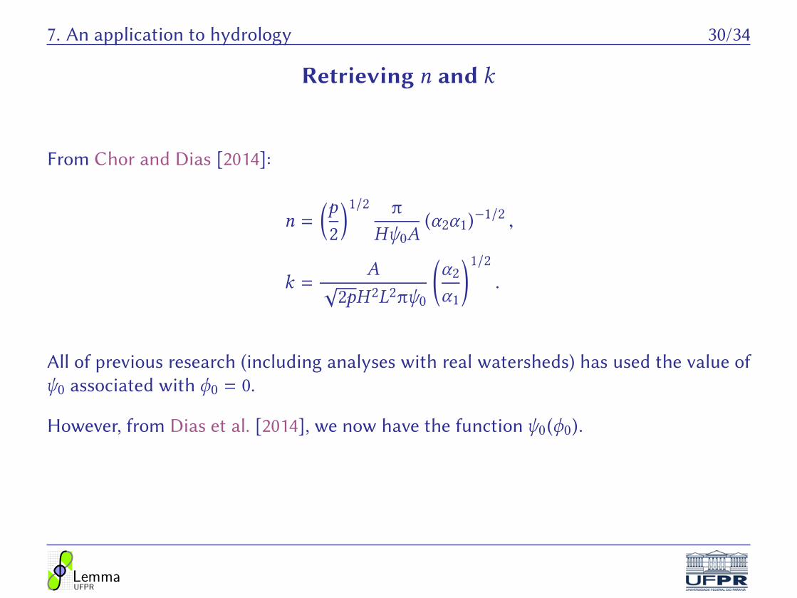
Retrieving n and k

From Chor and Dias [2014]:

n =(p2

)1/2 π

Hψ0A(α2α1)

−1/2 ,

k =A√

2pH 2L2πψ0

(α2α1

)1/2.

All of previous research (including analyses with real watersheds) has used the value ofψ0 associated with ϕ0 = 0.

However, from Dias et al. [2014], we now have the functionψ0(ϕ0).

LemmaUFPR


E�ect of changingψ0.

0.0

0.2

0.4

0.6

0.8

1.0

1.2

0.0 0.1 0.2 0.3 0.4 0.5 0.6 0.7 0.8 0.9 1.0

φ0

k0(φ0)/k0

k0(φ0 = 0)/k0 (BN77's method)

0.0

0.2

0.4

0.6

0.8

1.0

1.2

0.0 0.1 0.2 0.3 0.4 0.5 0.6 0.7 0.8 0.9 1.0

φ0

ne(φ0)/ne

ne(φ0 = 0)/ne (BN77's method)

LemmaUFPR

8. Conclusions 32/34

8. Conclusions

You may know more about this talk in:

Tomás Luís Guimarães Chor, Nelson Luís Dias, and Ailin Ruiz de Zarate. Solução em sérieda equação de boussinesq para fluxo subterrâneo utilizando computação simbólica. InAnais, XX Simpósio Brasileiro de Recursos hídricos, Bento Gonçalves, RS, 2013b

T. Chor, N. L. Dias, and A. R. de Zárate. An exact series and improved numerical and ap-proximate solutions for the boussinesq equation. Water Resour. Res., 49:7380–7387, 2013a.doi: 10.1002/wrcr.20543

N. L. Dias, T. Chor, and A. R. de Zárate. A semi-analytical solution for the boussinesqequation with non-homogeneous constant boundary conditions. Water Resour. Res., 50(8):6549–6556, 2014. doi: 10.1002/2014WR015437

T. L. Chor and N. L. Dias. A simple generalization of the brutsaert and nieber analysis.Hydrology and Earth System Sciences Discussions (Online), 11:12519–12530, 2014

LemmaUFPR


Closing remarks

• To this day, the analytical (series and asymptotic) solutions of Blasius are a powerfultool, not only for Boundary-Layer Theory, but for a completely unrelated problem,the Boussinesq non-linear equation.

LemmaUFPR


Closing remarks


• Unfortunately, the initial conditionψ0 still needs to be calculated numerically (but weare working on it!).

LemmaUFPR


Closing remarks



• A host of analytical and semi-analytical techniques (complex plane integration andCauchy’s Theorem; Padé approximations; asymptotic analysis of di�erential equa-tions) are needed to make analytical solutions useful for groundwater problems.

LemmaUFPR


Closing remarks




• We must recognize that the first strides (Blasius, Polubarinova-Kochina, Heaslet andAlksne) were the largest, but the recent improvements promise a much wider scopeof applications and unprecedented (maybe not needed in Engineering) accuracy.

LemmaUFPR


Closing remarks




• We must recognize that the first strides (Blasius, Polubarinova-Kochina, Heaslet andAlksne) were the largest, but the recent improvements promise a much wider scopeof applications and unprecedented (maybe not needed in Engineering) accuracy.

• I leave you with the most accurate (31 digits) estimate of Blasius’s constant for the

shear stress in a laminar boundary-layer, from Chor et al. [2013a]:

κ = 0.33205733621519629893718005933892

LemmaUFPR


Many thanks

. . . for your a�ention!

LemmaUFPR


Many thanks

. . . for your a�ention!

�estions?

LemmaUFPR


References

*References

H. Blasius. Grenzschichten in flüssigkeiten mit kleiner reibung. Z. Math.Phys., 56:1–37, 1908.

J. Boussinesq. Sur le débit, en temps de sécheresse, d’une source alimentéepar une nappe d’eaux d’infiltration. C. R. Hebd. Seances Acad. Sci, 136:1511–1517, 1903.

M. J Boussinesq. Recherches théoriques sur l’écoulement des nappes d’eauinfiltrées dans le sol sur le débit des sources. J des Mathématiques Pureset Appliquées, 5éme Sér., 10:5–78, 1904.

J. P. Boyd. The Blasius function: Computations before computers, the

LemmaUFPR


value of tricks, undergraduate projects, and open research problems.SIAM Rev., 50(4), 2008.

W. Brutsaert and J L. Nieber. Regionalized drought flow hydrographs froma mature glaciated plateau. Water Resour. Res., 13:637–643, 1977.

T. Chor, N. L. Dias, and A. R. de Zárate. An exact series and improved nu-merical and approximate solutions for the boussinesq equation. WaterResour. Res., 49:7380–7387, 2013a. doi: 10.1002/wrcr.20543.

T. L. Chor and N. L. Dias. A simple generalization of the brutsaert andnieber analysis. Hydrology and Earth System Sciences Discussions (On-line), 11:12519–12530, 2014.

Tomás Luís Guimarães Chor, Nelson Luís Dias, and Ailin Ruiz de Zarate.Solução em série da equação de boussinesq para fluxo subterrâneo uti-

LemmaUFPR


lizando computação simbólica. In Anais, XX Simpósio Brasileiro de Re-cursos hídricos, Bento Gonçalves, RS, 2013b.

N. L. Dias, T. Chor, and A. R. de Zárate. A semi-analytical solutionfor the boussinesq equation with non-homogeneous constant bound-ary conditions. Water Resour. Res., 50(8):6549–6556, 2014. doi: 10.1002/2014WR015437.

Max A. Heaslet and Alberta Alksne. Di�usion from a fixed surface with aconcentration-dependent coe�icient. J. SoC. INDUST. APPL. MATH., 9:584–596, 1961. doi: {10.1137/0109049}.

W. L. Hogarth and J Y. Parlange. Solving the Boussinesq equation usingsolutions of the Blasius equation. Water Resour. Res., 35(3):885–887, 1999.

Hassan Ali Ibrahim and Wilfried Brutsaert. Inflow hydrographs from large

LemmaUFPR


unconfined aquifers. J. Irrig. Drain. Div., Proc. ASCE, 91(IR2):21–38, June1965.

L. A. Melsen, A. J. Teuling, S. W. van Berkum, P. J. J. F. Torfs, and R. Ui-jlenhoet. Catchments as simple dynamical systems: A case study onmethods and data requirements for parameter identification. Water Re-sources Research, 50(7):5577–5596, 2014. ISSN 1944-7973. doi: 10.1002/2013WR014720. URL http://dx.doi.org/10.1002/2013WR014720.

Raphaël Mutzner, Enrico Bertuzzo, Paolo Tarolli, Steven V. Weijs, Lu-dovico Nicotina, Serena Ceola, Nevena Tomasic, Ignacio Rodriguez-Iturbe, Marc B. Parlange, and Andrea Rinaldo. Geomorphic signatureson brutsaert base flow recession analysis. Water Resources Research,49(9):5462–5472, 2013. ISSN 1944-7973. doi: 10.1002/wrcr.20417. URLhttp://dx.doi.org/10.1002/wrcr.20417.

P. YA. Polubarinova-Kochina. Theory of ground water movement. Princeton

LemmaUFPR

http://dx.doi.org/10.1002/2013WR014720

http://dx.doi.org/10.1002/wrcr.20417


University Press, Princeton, New Jersey, 1962. ISBN 9780783793283. URLhttp://books.google.ca/books?id=idOVPQAACAAJ.

B. Punnis. Zur di�erentialgleichung der pla�engrenzschicht von Blasius.Archiv der Mathematik, 7:165–171, 1956.

K. Töpfer. Bemerkung zu dem aufsatz von H. Blasius: Grenzschichten inflüssigkeiten mit kleiner reibung. Z. Math. Phys., 60:397–398, 1912.

Olivier Vannier, Isabelle Braud, and Sandrine Anquetin. Regional estima-tion of catchment-scale soil properties by means of streamflow recessionanalysis for use in distributed hydrological models. Hydrological Pro-cesses, 28(26):6276–6291, 2014. ISSN 1099-1085. doi: 10.1002/hyp.10101.URL http://dx.doi.org/10.1002/hyp.10101.

Rameshwar D. Verma and Wilfried Brutsaert. Unsteady free surface

LemmaUFPR

http://books.google.ca/books?id=idOVPQAACAAJ

http://dx.doi.org/10.1002/hyp.10101


ground water seepage. J. Hydraul. Div., Proc. ASCE, 97(HY8):1213–1229,August 1971.

LemmaUFPR

recent progress in analytical solutions of the boussinesq ... · recent progress in analytical...

Documents