"Discrete Dislocation Plasticity" Cambridge

Thursday 1 July - Friday 2 July, 2004

benoit.devincre@onera.fr

Recent progress on discretedislocation dynamics simulations

Laboratoire d’Etude des Microstructures, CNRS-ONERAF-92322 Chatillon Cedex, FRANCE

Outline• A short review of DDD evolutions• 3D-DDD

– Piecewise line models– Materials specificity

• Slip system symmetry• Contact reactions (junctions)• Velocity laws• Standing problems

– Boundary Problems• PBC• Superposition or Eigenstrain methods ?

– Computational issues• Fast multipole methods (Greengard)• Parallelization

• 2D v.s. 3D and 2.5-DDD• Concluding remarks

1966� 1986 �����1992 1998������2D inplane 2D outplane 3D (lattice) 3D (continuous)

Patterning(1/ r)

Discrete Dislocation Dynamics main dates

HardeningLine tension

Obstacle pinning

“French touch”multi-slip

ASCI programbcc

1995 1998 �����2001 2003������Superposition Strong FE

couplingPBC //

Anisotropicelasticity

Boundaryproblem

Mean freepath Hardening

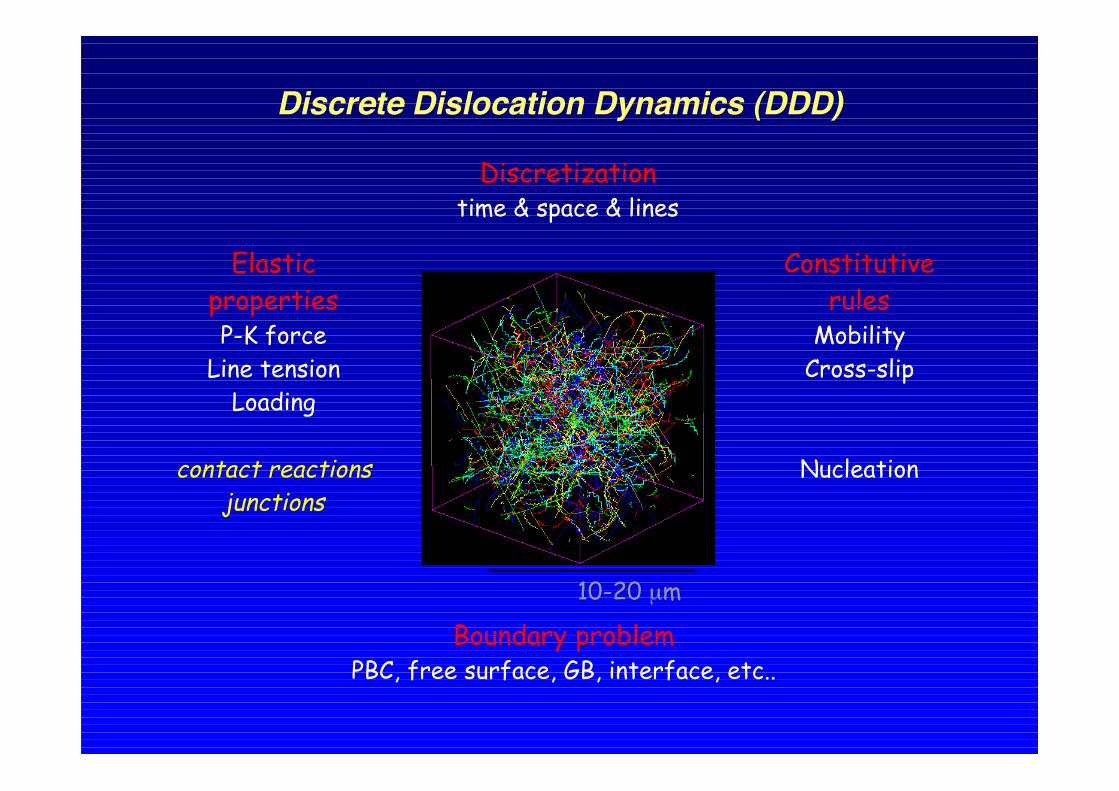
Discretizationtime & space & lines

ElasticpropertiesP-K force

Line tensionLoading

contact reactionsjunctions

Constitutiverules

MobilityCross-slip

Nucleation

10-20 µm

Discrete Dislocation Dynamics (DDD)

Boundary problemPBC, free surface, GB, interface, etc..

nm µm mm mSpace and line discretization

Lattice-based models Quasi-continuous models

(Forest zipping-unzipping) (Orowan mechanism)

MDDD

FE

Code simplicityslip properties

Dislocation self stress fieldCPU (time step ?)

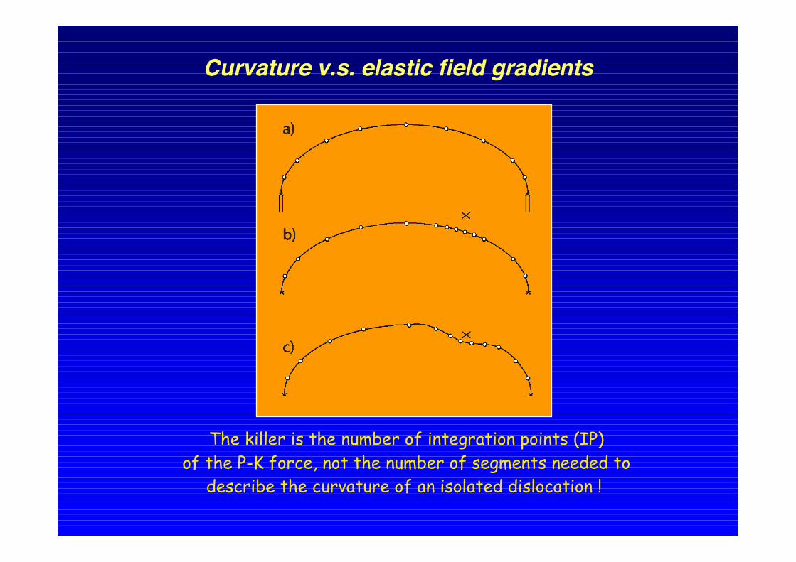
Curvature v.s. elastic field gradients

The killer is the number of integration points (IP)of the P-K force, not the number of segments needed to

describe the curvature of an isolated dislocation !

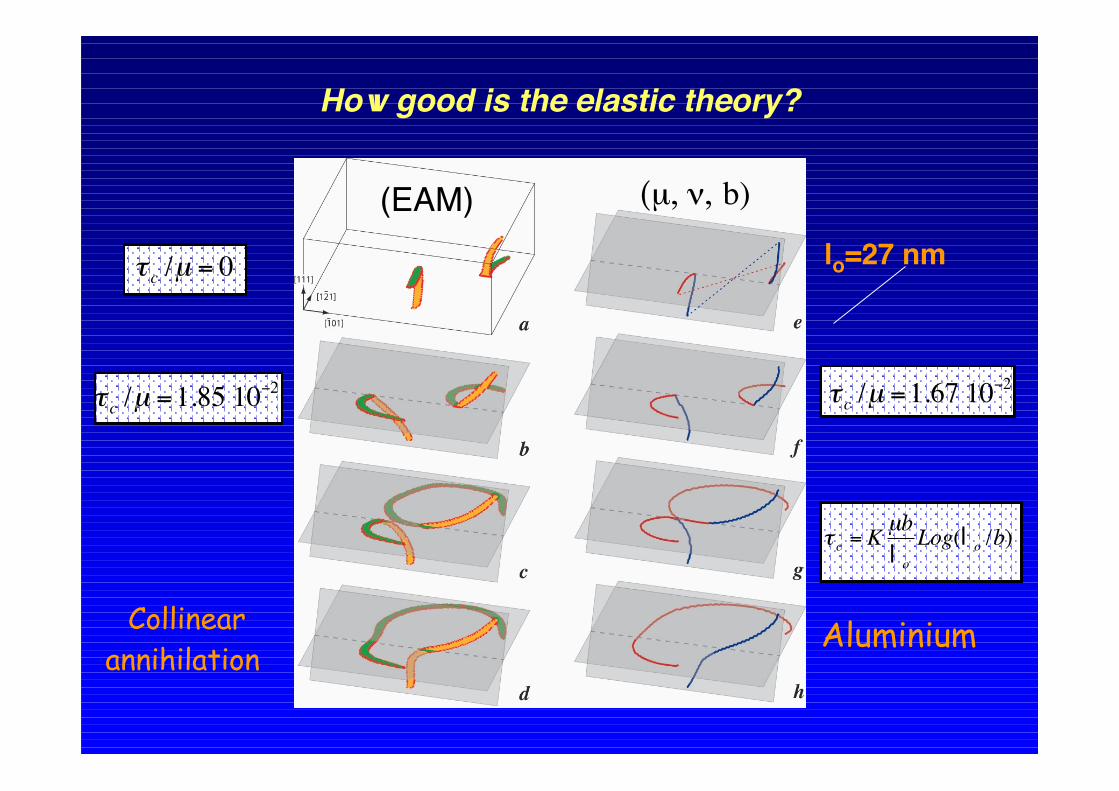
How good is the elastic theory?

€

τ c /µ =1.85 10−2

€

τ c /µ =1.67 10−2

lo=27 nm

€

τ c = K µbl o

Log(l o /b)

€

τ c /µ = 0

Aluminium

(EAM) (µ, ν, b)

Collinearannihilation

Contact reactions modeling

jonction CrossState

repulsion

IP optimization Line tension at triple nodes

Collinear annihilation

aij - Interaction coefficients - FCCs(model simulations)

Measurement:

a1copla: coplanar

a3: Lomera2: glissilea1ortho: Hirth

€

asu = (σ s / ρu

u∑ )2

Hirth (a1ortho= 0.051) Glissile (a2= 0.075) Lomer (a3= 0.084)

a0: self

b

b

b

b bb

c-s

a1coli: annihilation

acoli= 1.265

screw

edge

screw

edge

a1 a2

c

Vscrew << Vnon-screw

−

Δ−=

q

peff

o

o kTG

ll

vv )(1exp0

0

τ

τ

€

v0 = 1014s−1

ΔG0 = 1.06 eV : Total energy

τ0 = 260 MPa : CRSS at 0 K

p = 0.757, q = 1.075

Velocity laws

Eg: Zirconium (prismatic)

€

v =τ eff bB(T)

Viscous drag

Lattice friction

Segments length influence(double kink free path)

Internal stress fluctuations!

Technical standing problemsin dislocation properties modeling

• Cross-slip in non-fccs• Climb• Nucleation criteria• Transmission criteria• Jogs and kinks in materials with lattice friction• Over-damped motion approximation

Size effects (DDD+FE) Loading (DDD+FE)Bulk (DDD)

Boundary value problem

10µm

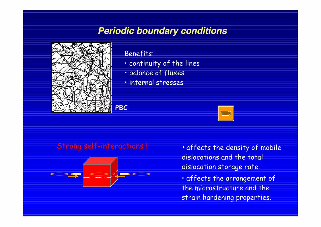
Benefits:• continuity of the lines• balance of fluxes• internal stresses

Periodic boundary conditions

PBC

Strong self-interactions ! • affects the density of mobiledislocations and the totaldislocation storage rate.• affects the arrangement ofthe microstructure and thestrain hardening properties.

This quantity must be calculated beforecomputations for each active slip systemT

Dislocation mean free path

€

huLx + kvLy + lwLz = 0

€

2λ = (uLx)2 +(vLy)2 + (wLz)2

self-annihilation distanceOrthorhombic box: Lx, Ly, Lz

Slip plane (h, k, l)

find 3 integers (u, v, w) such that

Isotropic Loop:

Anisotropic Loop:

€

λ =uLx

dx=

vLy

dy=

wLz

dzwith (dx,dy,dz) the fastgliding direction

(first-degree Diophantineequation)

(Madec, Devincre, Kubin:IUTAM 2003 proceedings, Kluwer Eds.)

(Monnet, Devincre, Kubin: Acta Mater. 2004)

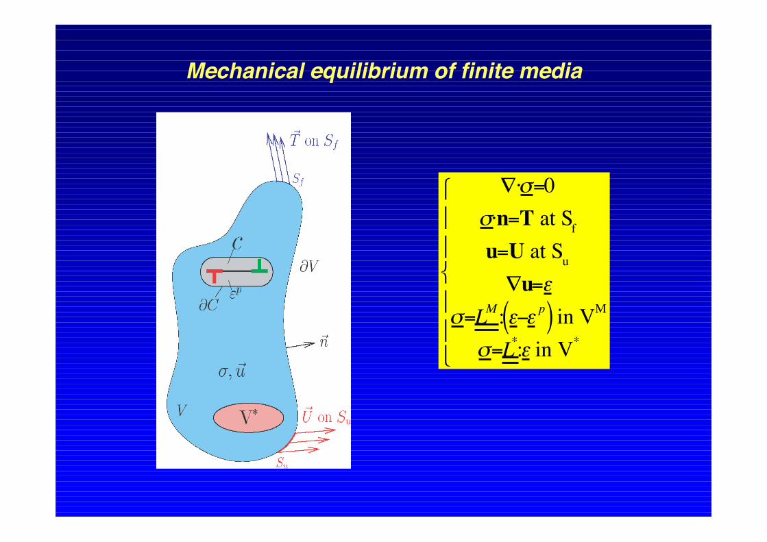
Mechanical equilibrium of finite media

€

∇⋅σ=0σ⋅n=T at Sf

u=U at Su

∇u=εσ=LM : ε−ε p( ) in VM

σ=L*:ε in V*

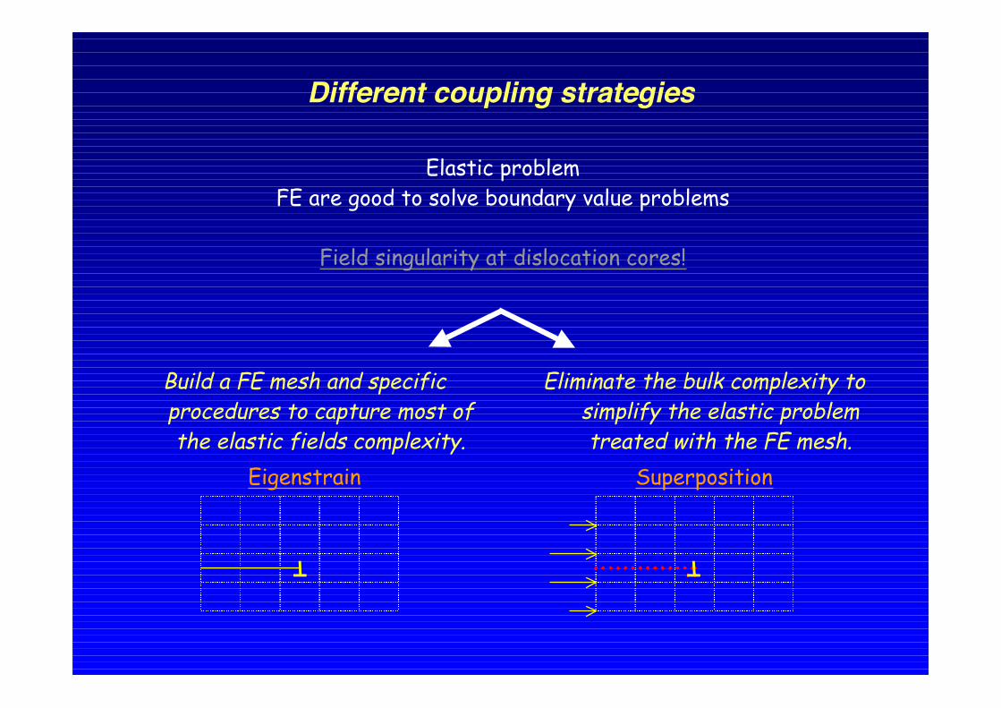
Different coupling strategies

Build a FE mesh and specificprocedures to capture most ofthe elastic fields complexity.

Eigenstrain

Eliminate the bulk complexity tosimplify the elastic problemtreated with the FE mesh.

Superposition

Elastic problem FE are good to solve boundary value problems

Field singularity at dislocation cores!

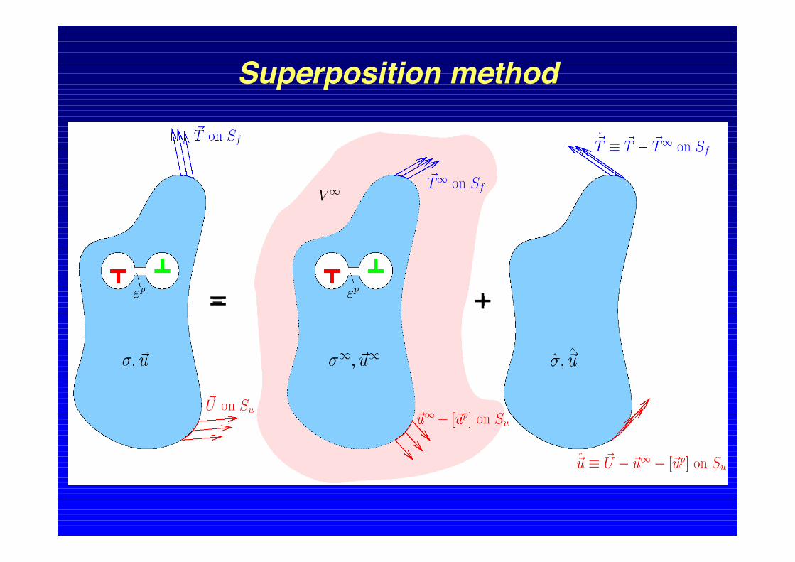
Superposition method

€

∇⋅ ˆ σ =0ˆ σ ⋅n=T−σ∞⋅n at Sf

ˆ u =U−u∞- up[ ] at Su

∇ ˆ u =ˆ ε ˆ σ =LM :ˆ ε in VM

ˆ σ =L*:ˆ ε +(L*−LM):ε∞ in V*

= +

Eigenstrain (homogenisation) method

bb Plastic strain induced by the

motion of each segment "i” atthe Gauss points ",e" of the FE

mesh and at time "t"

€

Δγn,ei =

bi/h( ) Vint,ei

VG,e

Δε,ep= Δγn,e

i

i∑ li⊗ni( )

sym

ε,ep= Δε,e

p

t∑

Homogenisation slab ofthickness h=1.5 (VG,e)1/3

is OK with elements of 20nodes and 27 Gauss points.

Strength and weakness of DDD-FE coupling

• Computer efficiency!– FE computations are faster than DDDs

• Isotropic or anisotropic elasticity !– Analytical forms for the displacement field

• Large deformation and surface roughness !– homogenisation or re-meshing

• Elastic inclusions !• Interpolation and shape functions!

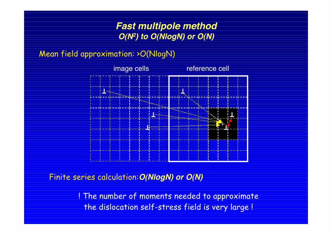
Fast multipole methodO(N2) to O(NlogN) or O(N)

reference cellimage cells

Mean field approximation: >O(NlogN)

Finite series calculation:O(NlogN) or O(N)

! The number of moments needed to approximatethe dislocation self-stress field is very large !

Parallel DDD codes

The LLNL battlefield :-)Size of dislocation patterns approx 1µm

Simulation box L=10µm

Dislocation density ρ=1012m-2

Length of dislocation line Γ=ρL3=10-3m

Discretization length d=10 nm

Number of segments N=Γ/d=105

One processor can only handle efficiently 103-104 segments

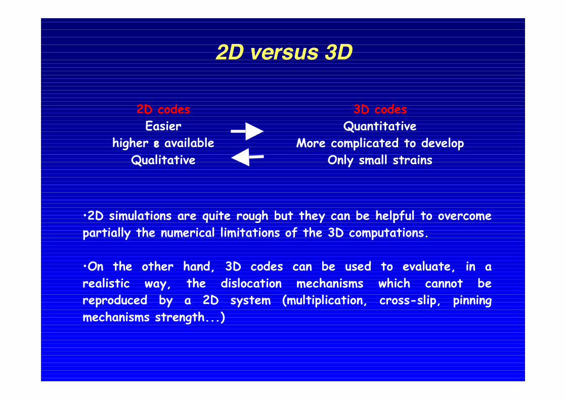
•2D simulations are quite rough but they can be helpful to overcomepartially the numerical limitations of the 3D computations.

•On the other hand, 3D codes can be used to evaluate, in arealistic way, the dislocation mechanisms which cannot bereproduced by a 2D system (multiplication, cross-slip, pinningmechanisms strength...)

2D codesEasier

higher ε availableQualitative

3D codesQuantitative

More complicated to developOnly small strains

2D versus 3D

Dislocation patterning in double slip

s

Multiplication

Reactions

Dipoles

Junctions

Interaction

Velocity

Annihilation

homogenization(cross-slip)

€

τint ,τapp,T( )€

τ j =βT

=βµbρlocal−1/2 ln(

ρlocal−1/2

b)

€

Δρs

Δt= M˙ γ s + Sources

2.5 DDD simulation

(3D-DDD)€

M = 2.1015

€

β = 0.046

€

h =dσdε

=dσdρ

dρdε

Forest modeland

Strain hardeningflow stress - junction strengthening multiplication rate - recovery

2.0

1.5

1.0

0.5

0.0τ/

µ (

10−3

)0.350.300.250.200.150.100.050.00

b/λ (10−3)

2.0

1.5

1.0

0.5

0.0τ/

µ (

10−3

)0.350.300.250.200.150.100.050.00

b/λ (10−3)

€

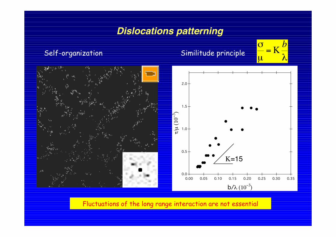
σµ

=K bλ

K=15

Similitude principle

Dislocations patterning

Self-organization

Fluctuations of the long range interaction are not essential

Concluding remarks

• The elastic theory of dislocations is powerful• Material specificities are coming up from the core properties• PBC are useful, but dangerous• Solving boundary value problems in 3D is a tough job, still in

progress.• Thanks to multipole algorithm and // codes, larger plastic

strains should be available in the near future.• Need for a rigorous validation and intercomparison of the

various approaches currently utilized.