recentered influence functions (rif) in stata - rif-regression and rif-decomposition ·...
TRANSCRIPT

Recentered Influence Functions (RIF) in StataRIF-regression and RIF-decomposition
Fernando Rios-Avila 1
1Levy Economics InstituteBard College
Stata Conference-Chicago 2019
Rios-Avila (Levy) RIF Stata Chicago 2019 1 / 47

Table of Contents
1 Prologue
2 Introduction
3 How to compare distributional statistics?
4 What are IFs & RIFs? why are they useful?
5 How are RIF’s estimated? grifvar()
6 RIF Regression: rifhdreg
7 RIF Decomposition: oaxaca rif
8 Latest Extensions: rifhdreg II
9 Conclusions
Rios-Avila (Levy) RIF Stata Chicago 2019 2 / 47

Table of Contents
1 Prologue
2 Introduction
3 How to compare distributional statistics?
4 What are IFs & RIFs? why are they useful?
5 How are RIF’s estimated? grifvar()
6 RIF Regression: rifhdreg
7 RIF Decomposition: oaxaca rif
8 Latest Extensions: rifhdreg II
9 Conclusions
Rios-Avila (Levy) RIF Stata Chicago 2019 3 / 47

Prologue
Interested in the commands. Download it from ssc: ssc install rif
Latest Files: https://bit.ly/2NFM3cH
Rios-Avila (Levy) RIF Stata Chicago 2019 4 / 47

Table of Contents
1 Prologue
2 Introduction
3 How to compare distributional statistics?
4 What are IFs & RIFs? why are they useful?
5 How are RIF’s estimated? grifvar()
6 RIF Regression: rifhdreg
7 RIF Decomposition: oaxaca rif
8 Latest Extensions: rifhdreg II
9 Conclusions
Rios-Avila (Levy) RIF Stata Chicago 2019 5 / 47

Introductions: Why ?
Once upon a time (2011), I was young(er), and came across a paper:Firpo, Fortin and Lemieux (2009): Unconditional QuantileRegressions (UQR).
The premise was simple: A regression framework analysis to explorefactors behind changes across the unconditional distributions(quantiles).
Similar (Conditional) Quantile regression, but not quite the same.
As many people. Sat down, read the paper and its companions manytimes. After understanding what it did, and apply it for mydissertation. (-rifreg-)
Rios-Avila (Levy) RIF Stata Chicago 2019 6 / 47

Introduction: Why?
Few years later(2017), couple of papers with the method, decided toteach it in my econometrics class. There was a problem.
Implementations of UQR in Stata were limited: -rifreg-, -xtrifreg-,-rifireg-. There was no ”easy” applications for decompositions.
I had programs that were too crude and clunky. Hard to share withstudents.
So what to do: if the solution does not exist yet. Solve it yourself!
Rios-Avila (Levy) RIF Stata Chicago 2019 7 / 47

Table of Contents
1 Prologue
2 Introduction
3 How to compare distributional statistics?
4 What are IFs & RIFs? why are they useful?
5 How are RIF’s estimated? grifvar()
6 RIF Regression: rifhdreg
7 RIF Decomposition: oaxaca rif
8 Latest Extensions: rifhdreg II
9 Conclusions
Rios-Avila (Levy) RIF Stata Chicago 2019 8 / 47

How to compare distributional statistics?
When comparing distributional statistics, one requires one of thefollowing items:
Collection of data: Y = [y1, y2, y3, ..., yN ]The Cumulative distribution function F (Y ) or FY
The probability density function f (Y ) or fY
Once any one of these three pieces is obtained, any distributionalstatistic (v()) can be easily estimated. And differences across twogroups can be obtained straight forward.
∆v = v(GY )− v(Fy )
Where ∆v is the change in v when Fy → Gy
Rios-Avila (Levy) RIF Stata Chicago 2019 9 / 47

Table of Contents
1 Prologue
2 Introduction
3 How to compare distributional statistics?
4 What are IFs & RIFs? why are they useful?
5 How are RIF’s estimated? grifvar()
6 RIF Regression: rifhdreg
7 RIF Decomposition: oaxaca rif
8 Latest Extensions: rifhdreg II
9 Conclusions
Rios-Avila (Levy) RIF Stata Chicago 2019 10 / 47

RIFs, IFs and Gateaux Derivative
Influence Functions (IF) can be thought as a generalization of theabove experiment.
It represents the re-scaled effect that a change in the distribution fromFy → Gy has on statistic v, when the change is infinitesimally small:
G yiY = (1− ε)FY + ε1yi
IF (yi , v(FY )) = limε→0
v(G yiY )− v(FY )
ε
And, as introduced by FFL(2009)
RIF (yi , v(FY )) = v(FY ) + IF (yi , v(FY ))
The contribution of yi to the statistic v()
Rios-Avila (Levy) RIF Stata Chicago 2019 11 / 47

Visual Example of the change in F
Rios-Avila (Levy) RIF Stata Chicago 2019 12 / 47

RIF’s Properties
RIF has the following characteristics:
RIF (yi , v(FY )) = v(FY ) + IF (yi , v(FY ))
E (RIF (yi , v(FY ))) = v(FY )
E (IF (yi , v(FY ))) = 0
Var(v(FY )) = E (IF (yi , v(FY ))2)
Rios-Avila (Levy) RIF Stata Chicago 2019 13 / 47

Why are they useful?
Visual tool to inspect data, analyze statistics robustness to outliers(Cowel and Flatchaire, 2007)
Simple estimation of standard errors of distributional statistic(Deville, 1999)
Analysis of unconditional partial effects on distributional statisticsbased on regression and decomposition analysis (FFL, 2009,2018)
Rios-Avila (Levy) RIF Stata Chicago 2019 14 / 47

Table of Contents
1 Prologue
2 Introduction
3 How to compare distributional statistics?
4 What are IFs & RIFs? why are they useful?
5 How are RIF’s estimated? grifvar()
6 RIF Regression: rifhdreg
7 RIF Decomposition: oaxaca rif
8 Latest Extensions: rifhdreg II
9 Conclusions
Rios-Avila (Levy) RIF Stata Chicago 2019 15 / 47

How are RIF’s Estimated?
The estimation of RIFs varies in complexity depending on the statisticof interest:Mean:
RIF (yi , µY ) = yi
Variance:RIF (yi , σ
2Y ) = (yi − µY )2
Quantile:
RIF (yi , qY (p)) = qY (p) +p − 1(y ≤ qY (p))
fY (qY (p))
But complexity increases for other statistics.
In Rios-Avila (2019) I provide a collection of RIFs for a large set ofdistribution statistics. They include the statistics from FFL(2018),Firpo and Pinto (2016), Chung and Vankerm (2018), Cowell andFlachaire (2007), Essama-Nssah and Lambert (2012) and Heckley etal (2016).
Rios-Avila (Levy) RIF Stata Chicago 2019 16 / 47

Using grifvar()
grifvar() is an addon for egen(), that can be used to estimate allRIF’s detailed in Rios-Avila(2019). It can be installed using (sscinstall rif)
The syntax is:egen new=rifvar(oldvar) [if/in], [by() weight()
rifoptions]
rifoptions: Mean, variance, Coefficient of variation,
standard deviation, quantile, Interquantile range,
interquantile ratio, Gini, etc
For further detail -help rifvar-
Rios-Avila (Levy) RIF Stata Chicago 2019 17 / 47

Example using grifvar
webuse nlswork, cleargen wage=exp(ln wage)egen rif gini=rifvar(wage), giniegen rif log=rifvar(wage), logvaregen rif varlog=rifvar(ln wage), varegen rif iqr=rifvar(ln wage), iqr(20 80)egen rif iqsr=rifvar(wage), iqsr(20 80)recode age (14/24=1 ”14-24”) (25/34=2 ”25-34”) (35/46=3 ”35-46”),gen(age g)egen rif gini age=rifvar(wage), gini by(age g)
Rios-Avila (Levy) RIF Stata Chicago 2019 18 / 47
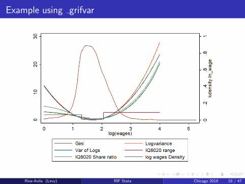
Example using grifvar
Rios-Avila (Levy) RIF Stata Chicago 2019 19 / 47

Example using grifvar
Rios-Avila (Levy) RIF Stata Chicago 2019 20 / 47

Example using grifvar
Bootstrap with INEQDECO vs Mean RIF
Rios-Avila (Levy) RIF Stata Chicago 2019 21 / 47

Table of Contents
1 Prologue
2 Introduction
3 How to compare distributional statistics?
4 What are IFs & RIFs? why are they useful?
5 How are RIF’s estimated? grifvar()
6 RIF Regression: rifhdreg
7 RIF Decomposition: oaxaca rif
8 Latest Extensions: rifhdreg II
9 Conclusions
Rios-Avila (Levy) RIF Stata Chicago 2019 22 / 47

RIF Regression: rifhdreg
FFL(2009) Introduced the a new type of quantile regression that theycall unconditional quantile regression. This was a special case of RIFregressions.
The core of the idea was:
In a linear regression y = b0 + b1 ∗ x1 + b2 ∗ x2 + e we are modelinghow changes in x’s may cause a change in y.RIF (yi , v(FY )) is the contribution of an observation yi has on theconstruction of statistic v.then, if we model RIF (yi , v(FY )) = a0 + a1 ∗ x1 + a2 ∗ x2 + e, we aremodeling how changes in X’s relate to the contributions of observationi to the statistic of interest.
FFL(2009) proposed using the RIF instead of IF. (No impact onregressions)
Rios-Avila (Levy) RIF Stata Chicago 2019 23 / 47

RIF Regression: rifhdreg
So now that we are modeling RIF’s as functions of X’s. Theinterpretation requires some care. why?
RIF (yi , v(FY )) = a0 + a1 ∗ x1 + a2 ∗ x2 + e
The simple partial effect tell us...nothing, except for few exceptions(for example Mean, FGT and Watts poverty indices).
∂RIF (.)
∂x1= a1
∂E (RIF (.)|x1, x2)
∂x1= a1
why? if x1 changes for person i, that persons influence on theoutcome will change in a1. But, in a population of millions, oneperson won’t make a difference on v.
Rios-Avila (Levy) RIF Stata Chicago 2019 24 / 47

RIF Regression: rifhdreg
Alternatively, if we take unconditional expectations:
E(RIF (yi , v(FY ))
)= E (a0 + a1 ∗ x1 + a2 ∗ x2 + e)
v(FY ) = a0 + a1 ∗ E (x1) + a2 ∗ E (x2)
So we can derive correct partial effect
∂v(FY )
∂E (x1)= a1
a1 is the effect that a unit change in the average value of E (x1) willhave on statistic v , assuming everything else constant.
For most v(), one needs to assumes everyone’s x change in 1 unit.
For Dummy variables, one needs to assume the change is in theProportion of people in a particular group.
Rios-Avila (Levy) RIF Stata Chicago 2019 25 / 47
RIF Regression: rifhdreg
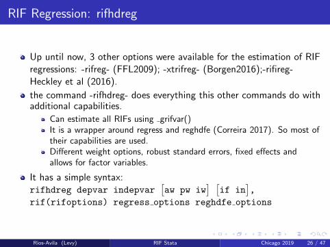
Up until now, 3 other options were available for the estimation of RIFregressions: -rifreg- (FFL2009); -xtrifreg- (Borgen2016);-rifireg-Heckley et al (2016).
the command -rifhdreg- does everything this other commands do withadditional capabilities.
Can estimate all RIFs using grifvar()It is a wrapper around regress and reghdfe (Correira 2017). So most oftheir capabilities are used.Different weight options, robust standard errors, fixed effects andallows for factor variables.
It has a simple syntax:rifhdreg depvar indepvar
[aw pw iw
] [if in
],
rif(rifoptions) regress options reghdfe options
Rios-Avila (Levy) RIF Stata Chicago 2019 26 / 47

rifhdreg: Example
RIF regression with rescaled RIF:rifhdreg wage age grade union tenure hours wks work,
rif(gini) scale(1000) robust
rifhdreg wage age grade union tenure hours wks work,
rif(ucs(80)) scale(100) robust
RIF regression with rescaled RIF and Fixed effects:rifhdreg wage age grade union tenure hours wks work,
rif(gini) scale(1000) vce(robust) abs(idcode) keepsingleton
rifhdreg wage age grade union tenure hours wks work,
rif(ucs(80)) scale(100) vce(robust) abs(idcode)
keepsingleton
Rios-Avila (Levy) RIF Stata Chicago 2019 27 / 47

RIF Regression: rifhdreg
Rios-Avila (Levy) RIF Stata Chicago 2019 28 / 47

RIF Regression: rifhdreg
(1) (2) (3) (4) (5) (6) (7)gini ucs80 lor20 mean X FE gini FE ucs80 FE lor20
age 4.905 0.350 -0.133 31.39 5.424 0.398 -0.134(0.548) (0.0470) (0.0110) (0.0454) (1.079) (0.0936) (0.0183)
grade 4.604 0.0708 -0.292(1.240) (0.108) (0.0256)
union 0.746 -0.501 -0.180 0.236 -13.91 -1.101 0.474(7.176) (0.630) (0.125) (0.00311) (7.065) (0.615) (0.153)
tenure -0.102 -0.129 -0.0854 4.003 0.644 -0.0584 -0.105(0.588) (0.0525) (0.0124) (0.0303) (1.006) (0.0887) (0.0189)
hours -3.142 -0.251 0.0643 36.82 -3.037 -0.263 0.0478(0.327) (0.0274) (0.00857) (0.0698) (0.552) (0.0473) (0.0115)
wks work -0.288 -0.0168 0.00848 63.29 -0.204 -0.0128 0.00510(0.103) (0.00885) (0.00225) (0.208) (0.105) (0.00913) (0.00218)
cons 185.2 35.34 15.28 218.9 34.80 12.31(18.44) (1.567) (0.497) (40.58) (3.511) (0.714)
N 18601 18601 18601 18601 18601 18601 18601rifmean 263.8 36.31 9.894 263.8 36.31 9.894
Standard errors in parentheses
Rios-Avila (Levy) RIF Stata Chicago 2019 29 / 47

Table of Contents
1 Prologue
2 Introduction
3 How to compare distributional statistics?
4 What are IFs & RIFs? why are they useful?
5 How are RIF’s estimated? grifvar()
6 RIF Regression: rifhdreg
7 RIF Decomposition: oaxaca rif
8 Latest Extensions: rifhdreg II
9 Conclusions
Rios-Avila (Levy) RIF Stata Chicago 2019 30 / 47

RIF Decomposition: oaxaca rif
-rifhdreg- provides a simple framework for analyzing the impact ofchanges in the distribution of X’s on distributional statistics, at themargin. (RIF’s are Local linear approximations)
Large changes in distributions require other methods, for exampledecomposition methods: Oaxaca Blinder
The premise, allow for all distributions of X’s to change between twogroups.
As long as the conditional independence assumptions holds, we canapply OB to decompose differences in statistics as functions ofdifferences in characteristics, and differences in returns to thosecharacteristics.
Rios-Avila (Levy) RIF Stata Chicago 2019 31 / 47

RIF Decomposition: oaxaca rif
The simple OB framework:
∆v = v(Hy )− v(Fy )
∆v = βhX h − βf X f
∆v = βh(X h − X f )− (βh − βf )X f
This assumes a linear counterfactual v(CFy ) = βhX f
A better counterfactual can be obtained using IPW (ω(x)).
∆v = v(∫
(HY |X ∗ dHX ))− v(∫
(FY |X ∗ dFX ))
v(CFy ) = v(∫
(HY |X ∗ dFX ))
= v(∫
(HY |X ∗ω(x) ∗ dHX ))
= βcX c
Rios-Avila (Levy) RIF Stata Chicago 2019 32 / 47

RIF Decomposition: oaxaca rif
-oaxaca rif- is a wrapper around -oaxaca- (Jann 2008) thatimplements these two types of decompositions.
It basically estimates the appropriate RIFs, uses them as dependentvariables, and re-arranges the results.
the syntaxoaxaca rif depvar indepvar
[aw pw iw
] [if in
], by(var)
rif(rifoptions) IPW options oaxaca options
Many features of -oaxaca- are kept.
Rios-Avila (Levy) RIF Stata Chicago 2019 33 / 47

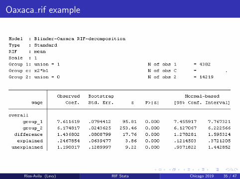
Oaxaca rif example
bootstrap:oaxaca rif wage age grade tenure hours wks work,
rif(mean) by(union) swap w(1)
bootstrap: oaxaca rif wage age grade tenure hours wks work,
rif(mean) by(union) rwlogit(age grade tenure hours
wks work) swap w(1)
bootstrap: oaxaca rif wage age grade tenure hours wks work,
rif(gini) by(union) rwlogit(age grade tenure hours
wks work) scale(1000) swap w(1)
bootstrap: oaxaca rif wage age grade tenure hours wks work,
rif(ucs(80)) by(union) rwlogit(age grade tenure hours
wks work) scale(100) swap w(1)
Rios-Avila (Levy) RIF Stata Chicago 2019 34 / 47
Oaxaca rif example
Rios-Avila (Levy) RIF Stata Chicago 2019 35 / 47

Oaxaca rif example
Rios-Avila (Levy) RIF Stata Chicago 2019 36 / 47

Oaxaca rif example
(1) (2) (3) (4) (5) (6)gini ucs80 lor20 q10 q50 q90
OverallGroup 1 246.1 34.72 10.35 1.394 1.919 2.446
(5.946) (0.536) (0.116) (0.00860) (0.00922) (0.00749)Group c 261.5 36.17 10.19 1.337 1.848 2.407
(9.477) (0.920) (0.168) (0.0107) (0.00987) (0.0107)Group 2 262.8 36.44 10.03 1.197 1.683 2.309
(2.029) (0.167) (0.0575) (0.00545) (0.00359) (0.00480)
ExplainedTotal -15.43 -1.446 0.161 0.0565 0.0710 0.0389
(4.287) (0.448) (0.0758) (0.00642) (0.00825) (0.00756)Pure explained -16.27 -1.451 0.227 0.0587 0.0634 0.0296
(3.761) (0.395) (0.0708) (0.00474) (0.00621) (0.00603)Specif err 0.840 0.00470 -0.0659 -0.00220 0.00765 0.00924
(0.686) (0.0655) (0.0174) (0.00659) (0.00413) (0.00516)
UnexplainedTotal -1.318 -0.273 0.161 0.140 0.166 0.0978
(9.336) (0.937) (0.169) (0.0122) (0.00957) (0.0114)Reweight err -2.119 -0.174 0.0451 0.00106 -0.000364 -0.00454
(0.705) (0.0647) (0.0139) (0.00119) (0.00157) (0.00160)Pure Unexplained 0.801 -0.0997 0.115 0.139 0.166 0.102
(9.394) (0.931) (0.168) (0.0123) (0.00959) (0.0119)
Standard errors in parentheses
Rios-Avila (Levy) RIF Stata Chicago 2019 37 / 47

Table of Contents
1 Prologue
2 Introduction
3 How to compare distributional statistics?
4 What are IFs & RIFs? why are they useful?
5 How are RIF’s estimated? grifvar()
6 RIF Regression: rifhdreg
7 RIF Decomposition: oaxaca rif
8 Latest Extensions: rifhdreg II
9 Conclusions
Rios-Avila (Levy) RIF Stata Chicago 2019 38 / 47

Other Extensions
Since its inception, early this year, a few other expansions have beenadded to this program. Some very recent.
-rifhdreg- It allows for SVY. Specially useful for the estimation ofstandard errors of distributional statistics.
-rifhdreg- adds ”over”. This may be used as a partial conditional RIF.Useful for standard errors across multiple groups.
-rifhdreg- can now estimate effects similar IPWRA treatment effects,using rwlogit or rwprobit. This is similar to Firpo and Pinto (2016).Allows for att, ate and atu. Useful for analyzing Inequality treatmenteffects
Rios-Avila (Levy) RIF Stata Chicago 2019 39 / 47

Other Extensions
-rifsureg-. This would the the equivalent to sqreg, but unconditionalquantile regressions.
Handy for making plots across quantiles.
-rifsureg2- is similar to rifsureg, but allows to simultanously estimateRIF regressions for non colinear models.
-uqreg- Stand alone command to estimate Unconditional Partialeffects for UQR with alternative model specifications(logit/probit/other)
Rios-Avila (Levy) RIF Stata Chicago 2019 40 / 47

rifsureg: Example
rifsureg ln wage age grade union tenure hours wks work,
qnts(10(10)90)
margins, dydx(grade) nose
marginsplot
Rios-Avila (Levy) RIF Stata Chicago 2019 41 / 47

rifsureg: Example
Rios-Avila (Levy) RIF Stata Chicago 2019 42 / 47

Table of Contents
1 Prologue
2 Introduction
3 How to compare distributional statistics?
4 What are IFs & RIFs? why are they useful?
5 How are RIF’s estimated? grifvar()
6 RIF Regression: rifhdreg
7 RIF Decomposition: oaxaca rif
8 Latest Extensions: rifhdreg II
9 Conclusions
Rios-Avila (Levy) RIF Stata Chicago 2019 43 / 47

Conclusions
RIF and IF are powerful tools for analyzing and visualizingdistributional statistics.
The three main commands presented today ( grifvar, rifhdreg,oaxaca rif) aim to facilitate the use of RIF’s for this type of analysis
Questions, comments and suggestions are welcome.
Thank you
Latest Files: https://bit.ly/2NFM3cH
Rios-Avila (Levy) RIF Stata Chicago 2019 44 / 47

References
Borgen, Nicolai T. 2016. ”Fixed effects in Unconditional QuantileRegression.” The Stata Journal no. 16 (2):403-415.
Chung, Choe, and Philippe Van Kerm. 2018. ”Foreign Workers and theWage Distribution: What Does the Influence Function Reveal.”Econometrics no. 6 (2):28.
Cowell, F. and E. Flachaire (2007). ’Income Distribution and InequalityMeasurement: The problem of Extreme Values.’ Journal of Econometrics,141(2):1044-1072.
Correira, Sergio. 2017. Linear Models with High-Dimensional FixedEffects: An Efficient and Feasible Estimator. In Working Paper. Deville,J.-C. 1999, ‘Variance estimation for complex statistics and estimators:linearization and residual techniques’, Survey Methodology 25, 193–204
Rios-Avila (Levy) RIF Stata Chicago 2019 45 / 47

References
Essama-Nssah, B. and Lambert, P. J. (2012), Influence functions forpolicy impact analysis, in J. A. Bishop and R. Salas, eds, ‘Inequality,Mobility and Segregation: Essays in Honor of Jacques Silber’, Vol. 20 ofResearch on Economic Inequality, Emerald Group Publishing, chapter 6,pp. 135–159
Firpo, S., Fortin, N. M. and Lemieux, T. (2009), ‘Unconditional quantileregressions’, Econometrica 77(3), 953–973.
Firpo, S., Fortin, N. M. and Lemieux, T. (2018), ‘Decomposing WageDistributions using Recentered Influence Functions Regressions’,Econometrics 6(41).
Firpo, S. P., and C. Pinto. (2016). ”Identification and Estimation ofDistributional Impacts of Interventions Using Changes in InequalityMeasures.” Journal of Applied Econometrics no. 31 (3):457-486
Jann, Ben. 2008. ”The Blinder-Oaxaca decomposition for linearregression models.” Stata Journal no. 8 (4):453-479.
Rios-Avila (Levy) RIF Stata Chicago 2019 46 / 47

References
Heckley, G., U.-G. Gerdtham, and G. Kjellsson. 2016. ”A GeneralMethod for Decomposing the Causes of Socioeconomic Inequality inHealth.” Journal of Health Economics. 48:89-106.
Rios-Avila, F. 2019. ”Recentered Influence Functions in Stata: Methodsfor Analyzing the Determinants of Poverty and Inequality” Working Paper927. Levy Economics Institute.
Rios-Avila (Levy) RIF Stata Chicago 2019 47 / 47