Reconciling Theoretical and Empirical

Human Capital Earnings Functions

Margaret Stevens

Nuffield College, Oxford

January 2000

Abstract

To interpret estimates of empirical earnings functions, and to resolve sample selection

problems such as "tenure bias", the wage determination process must be specified.

This paper shows that an earnings function can be interpreted as a wage offer in a

labour market auction in which the worker accepts the highest offer received. The

elasticity of the wage is one with respect to general human capital, and less than one

for specific capital. There is a sample selection problem because only accepted offers

are observed. This causes underestimation of the return to specific capital in a cross-

sectional earnings regression.

JEL Classification: J31

1

Reconciling Theoretical and Empirical

Human Capital Earnings Functions

Margaret Stevens

January 2000

1. Introduction

Estimation of empirical earnings functions, in which the logarithm of the wage

is regressed on measures of human capital for a cross-section of individuals, has been

a popular technique in labour market research since the work of Mincer (1974), yet

the earnings function has surprising little theoretical foundation. The original

Mincerian earnings function, containing measures of general human capital such as

years of schooling and experience, could be interpreted on the basis of competitive

theory as a technological relationship – the effect of human capital on productivity.

But the introduction of measures of specific human capital such as job tenure (Mincer

and Jovanovic, 1981) and, in more recent studies, of firm and industry variables as

well as individual variables, precludes the possibility of perfectly competitive wage

determination, and raises the question: what are we estimating?

The answer must be, as Topel (1991) assumes in his discussion of the potential

bias in the estimation of the returns to experience and tenure, that it is some kind of

wage determination function. But without some assumptions about the nature of the

wage determination process it is not possible to resolve the potential sample selection

problem in the estimation of earnings functions, nor is it clear how to interpret the

results.

The sample selection problem arises because of labour turnover. A worker

who is observed working for a particular firm does so as a result of choices made by

the worker and the firm: employment determination occurs jointly with wage

2

determination. To fully understand wages, we would like to know for each worker

what he would have earned if randomly assigned to any firm, but we only observe his

wage in the chosen firm.

The effect of sample selection on estimation of the return to tenure has been

particularly contentious. It has been argued that there is a positive bias, because tenure

may be correlated with unobserved match quality, or worker quality. In apparent

support of this argument, Abraham and Farber (1987) and Altonji and Shakotko

(1987) found the effect of tenure on wages to be almost insignificant after controlling

for unobserved heterogeneity. But Topel (1991) argued that a matching model of

turnover could be expected to cause a negative bias. Further, he criticised the methods

used in the earlier empirical papers to control for heterogeneity, and found a strong

positive tenure effect in his own analysis of the same data1.

These arguments have been conducted at an informal level. Most empirical

discussions of such problems make the implicit assumption of some kind of matching

process to determine employment, combined with an unspecified wage determination

process. The purpose of this paper is to present a formal model of wage and

employment determination in a labour market characterised by match heterogeneity,

which is consistent with the existing theory of general and specific human capital, and

which provides a precise interpretation of the empirical earnings function.

It is shown that the empirical earnings function can be regarded as a wage

offer function in a labour market auction in which employers make wage offers after

privately observing match quality, and workers accept the highest available offer. In

estimation of this function a sample selection problem arises because we observe only

those offers that are accepted. Sample selection bias leads to under-estimation of the

return to specific human capital in a least-squares wage regression.

3

2. Wage Determination with General and Specific Human Capital

2.1 Theoretical Models

Classical human capital theory suggests that wages respond fully to general

human capital but only partially to specific human capital (Becker, 1962; Oi, 1962).

The intuition that the return to specific human capital will be shared between worker

and firm, in the form of a wage higher than the worker's opportunity wage but lower

than productivity, was formalised by Hashimoto (1981). In Hashimoto's model, the

value of the worker's specific human capital is subject to shocks. Its ex-post value

within the firm (within-firm productivity) is observed only by the firm, and its ex-post

value elsewhere (the opportunity wage) is observed only by the worker. The

asymmetry of information may result in inefficient separation and loss of specific

capital; to minimise this loss it is desirable for the worker and firm to predetermine

the wage. Hashimoto derives the optimal predetermined wage; he does not prove

"sharing" in the sense that the wage lies strictly between the expected alternative wage

and expected productivity, but it can be shown that if the two shocks are identically

distributed2 then it will do so. In this model the external labour market is assumed to

be perfectly competitive, so that the return to general human capital accrues to the

worker.

Hashimoto's analysis was important because it showed that the wage of a

worker possessing specific human capital is determinate only under the assumption

that wage and employment decisions are affected by asymmetric information, but the

model begs some awkward questions. If specific human capital can have an ex-post

value in other firms, is it really specific? How can the firm be unaware of the worker's

alternative wage in a competitive labour market? These problems can be avoided as in

Carmichael's (1983) model by assuming instead that the worker experiences a taste

4

shock which affects his utility of remaining in the current firm. But with this

interpretation Hashimoto's model does not necessarily predict "sharing" unless we

make the rather arbitrary assumptions that the taste shock is proportional to the size of

the investment in specific human capital, and distributed independently but identically

to the productivity shock.

More importantly for the purpose of the present paper, it is clear that if

empirical earnings functions represent predetermined wage functions then there

cannot be a sample selection problem arising from employment choices, precisely

because the wage is predetermined, before the shocks which determine employment

decisions are realised. These shocks contribute some unobserved quality to the match;

they affect the separation decision and hence whether or not the wage is observed, but

have no effect on the wage itself. The predetermined wage reflects only the worker's

expected human capital, and observed wages are a random sample of predetermined

wages.

Thus, if we believe that we are estimating predetermined wage functions there

is no need to be concerned about sample selection bias in the estimation of returns to

human capital variables. But as noted by Gibbons and Waldman (1999), post-training

wages are not typically specified in a contract. Moreover, the predetermined wage is

not the only type of employment contract possible for workers with specific human

capital. Wages may be determined ex-post by bargaining; when asymmetry of

information makes bargaining infeasible or costly, Hall and Lazear (1983) identified

other simple second-best contracts, such as allowing worker or firm to set the wage

unilaterally. There is no reason to suppose such contracts are less efficient than the

predetermined wage; Stevens (1994) shows that it may be preferable for the firm to

set the wage. Having chosen a mechanism for wage determination, a worker and firm

5

wishing to invest in specific human capital can determine their respective shares of

the expected match surplus under that contract, and bargain over the sharing of costs.

In this paper we develop an alternative to the predetermined wage model of

individual wage determination with specific and general human capital. The labour

market is characterised by match heterogeneity, to be consistent with the assumptions

underlying many empirical analyses. Like Hashimoto and Hall and Lazear we assume

that information asymmetries rule out bilateral bargaining; when the worker's

productivity varies across firms it is plausible to suppose that firms are not fully aware

of the alternative opportunities available to their employees, and that employees are

uncertain about their own value to their employer. In contrast to these two papers, the

external labour market is not perfectly competitive: this follows from the assumptions

that not only the worker's existing match but also his potential matches can vary in

quality, and that match productivity is the private information of the employer. We

then assume that the wage and employment of an individual worker are determined

according to a private-value auction mechanism: firms make simultaneous wage

offers and the worker accepts the highest offer. We will show that the labour market

auction results in sharing of the return to specific human capital3, but that in contrast

to the predetermined wage mechanism, there is a sample selection problem in the

estimation of the worker's share of the return.

2.2 Empirical Issues: Specific Capital, Match Quality and Tenure

The focus in recent empirical work has been on how to estimate the "true"

return to tenure. But the original question that Mincer and Jovanovic (1981) hoped to

address by including tenure in a cross-sectional earnings function was whether

specific human capital was an important determinant of wages. We need to know

whether employment relationships are characterised by a significant amount of

6

specific capital if, for example, we want to assess the gains and losses associated with

labour mobility and displacement.

There are two problems with the attempt to address these more fundamental

issues by estimating the return to tenure. First, if specific capital is normally acquired

during the first months of employment, a tenure variable measured in years may not

capture the pattern of accumulation very well. But also, it is argued (for example by

Abraham and Farber, 1987) that to estimate the "true" return to tenure it is necessary

to eliminate the effect on wages of an unobservable component of match quality,

constant throughout the duration of a match, and correlated with tenure because high

quality matches tend to last longer. But this kind of match quality is, by definition,

specific human capital: it is a permanent component of match productivity that would

be lost if the worker were to change employers. By removing it we underestimate the

extent of the worker's loss if match is destroyed. It might be preferable simply to

regard tenure as a rather poor proxy for the specific value of a match, picking up both

accumulating specific capital and permanent match quality.

Do these arguments mean that, whatever measure of specific human capital is

used in an earnings function, we should treat unobservable match quality as

unobservable specific capital? If so, we have a measurement error problem, not a

sample selection problem. The answer depends on what we want to estimate.

The approach we take in this paper is to use a static theoretical model of wage

determination, which could form the basis for a static empirical model. The

productivity of a match is determined by the worker's general and specific human

capital, which is assumed to be observable by all agents, and also affected by match

quality shocks of expected value zero, observed only by agents within the match.

Observable specific human capital is the amount by which the worker's productivity

7

in his present job is expected by all agents, ex-ante (before match qualities are

realised), to exceed his productivity elsewhere. It also represents the expectation by

agents in the external labour market of the worker's specific value, at the time when

wages are determined. We will suppose that the econometrician wishes to estimate the

worker's return to observable specific capital.

We also assume for simplicity that the econometrician has a perfect measure

of observable specific capital. It is straightforward to adapt the analysis in the usual

way if he observes it with error. We will return to discuss the implications of tenure

acting as a noisy signal of specific human capital in section 5 below.

3. An Auction Model of Wage Determination

Consider a worker attached to firm 0, who has general human capital g≥1, and

additional human capital k≥1 specific to firm 0. His productivity if he remains in firm

0 is v0, where:

ln ln ln lnv g k0 0= + + ε (1)

There are n alternative employers, and if he moves to an alternative firm i, his

productivity is vi:

ln ln lnv gi i= + ε (2)

εi >0 (i ≥0) represents the quality of his match with firm i, and is observable only by

firm i; g and k are common knowledge.

(1) and (2) capture the technological relationship between human capital and

productivity. Wages are determined through a first-price private-value auction: each

of the n+1 firms privately observes its own match quality, and makes a wage offer wi;

the worker accepts the highest offer.

8

3.1 Distributional Assumptions

Match qualities ε0, ε1,……εn are independent and identically distributed with

density and distribution functions f(ε) and F(ε). In order to apply results from auction

theory we make the following distributional assumptions:

D1: Finite support: ε ε εi ∈ [ , ]

D2: f(ε) >0

We also require:

D3: The density of lnεi is strictly log-concave.

A log-concave function is a function whose logarithm is concave. The class of

log-concave densities is a wide one, and includes the uniform distribution and the

truncated normal and log-normal distributions (Caplin and Nalebuff, 1991).

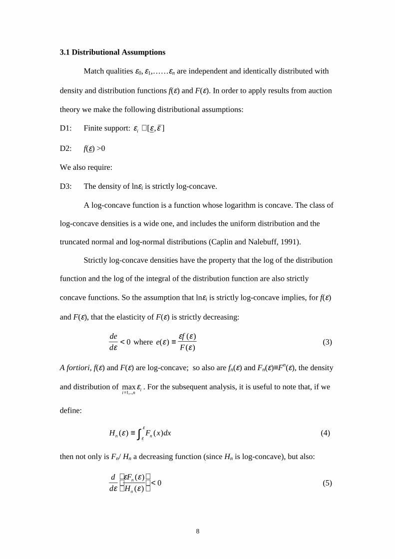
Strictly log-concave densities have the property that the log of the distribution

function and the log of the integral of the distribution function are also strictly

concave functions. So the assumption that lnεi is strictly log-concave implies, for f(ε)

and F(ε), that the elasticity of F(ε) is strictly decreasing:

de

dε< 0 where e

f

F( )

( )

( )ε

ε εε

≡ (3)

A fortiori, f(ε) and F(ε) are log-concave; so also are fn(ε) and Fn(ε)≡Fn(ε), the density

and distribution of max,..,i n

i=1ε . For the subsequent analysis, it is useful to note that, if we

define:

H F x dxn n( ) ( )εε

ε≡ ∫ (4)

then not only is Fn/ Hn a decreasing function (since Hn is log-concave), but also:

d

d

F

Hn

nεε ε

ε( )

( )

< 0 (5)

9

The proof of (5) is given in the appendix.

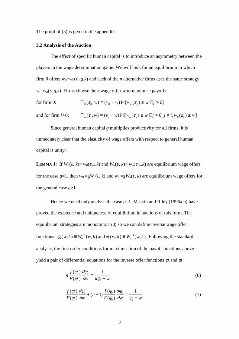
3.2 Analysis of the Auction

The effect of specific human capital is to introduce an asymmetry between the

players in the wage determination game. We will look for an equilibrium in which

firm 0 offers w0=w0(ε0,g,k) and each of the n alternative firms uses the same strategy

wi=wa(εi,g,k). Firms choose their wage offer w to maximise payoffs:

for firm 0: Π 0 0 0 0( , ) ( ) Pr[ ( ) ]ε εw v w w w ja j= − ≤ ∀ >

and for firm i>0: Π a i i a jw v w w w j j i w w( , ) ( ) Pr[ ( ) , , ( ) ]ε ε ε= − ≤ ∀ > ≠ ≤0 0 0

Since general human capital g multiplies productivity for all firms, it is

immediately clear that the elasticity of wage offers with respect to general human

capital is unity:

LEMMA 1: If W0(ε, k)≡ w0(ε,1,k) and Wa(ε, k)≡ wa(ε,1,k) are equilibrium wage offers

for the case g=1, then w0 =gW0(ε, k) and wa =gWa(ε, k) are equilibrium wage offers for

the general case g≥1.

Hence we need only analyse the case g=1. Maskin and Riley (1996a,b) have

proved the existence and uniqueness of equilibrium in auctions of this form. The

equilibrium strategies are monotonic in ε, so we can define inverse wage offer

functions: φ0 01( , ) ( , )w k W w k≡ − andφa aw k W w k( , ) ( , )≡ −1 . Following the standard

analysis, the first order conditions for maximisation of the payoff functions above

yield a pair of differential equations for the inverse offer functions φ0 and φa:

nf

F w k wa

a

a( )

( )

φφ

∂φ∂ φ

=−

1

0

(6)

f

F wn

f

F w wa

a

a

a

( )

( )( )

( )

( )

φφ

∂φ∂

φφ

∂φ∂ φ

0

0

0 11

+ − =−

(7)

10

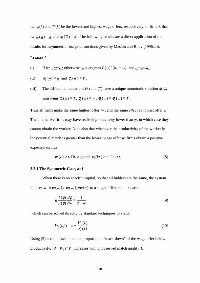
Let w(k) and w k( ) be the lowest and highest wage offers, respectively, of firm 0: that

is: φ ε0 ( )w = and φ ε0 ( )w = . The following results are a direct application of the

results for asymmetric first-price auctions given by Maskin and Riley (1996a,b):

LEMMA 2:

(i) If k=1, w=ε ; otherwise w F w k wn= −arg max ( ) ( )ε and ε <w<kε .

(ii) φa w w( ) = and φ εa w( ) = .

(iii) The differential equations (6) and (7) have a unique monotonic solution φ0,φa

satisfying φ ε0 ( )w = , φa w w( ) = , φ φ ε0 ( ) ( )w wa= = .

Thus all firms make the same highest offer w , and the same effective lowest offer w.

The alternative firms may have realised productivity lower than w, in which case they

cannot obtain the worker. Note also that whenever the productivity of the worker in

the potential match is greater than the lowest wage offer w, firms obtain a positive

expected surplus:

φ ε ε ε φ ε ε ε εa w k( ) ( )> ∀ > > ∀ ≥ and 0 (8)

3.2.1 The Symmetric Case, k=1

When there is no specific capital, so that all bidders are the same, the system

reduces with φ0(w,1)=φa(w,1)≡φ (w) to a single differential equation:

nf

F w w

( )

( )

φφ

∂φ∂ φ

=−1

(9)

which can be solved directly by standard techniques to yield:

WH

Fn

n0 1( , )

( )

( )ε ε

εε

= − (10)

Using (5) it can be seen that the proportional “mark-down” of the wage offer below

productivity, ( ) /ε ε−W0 , increases with unobserved match quality ε.

11

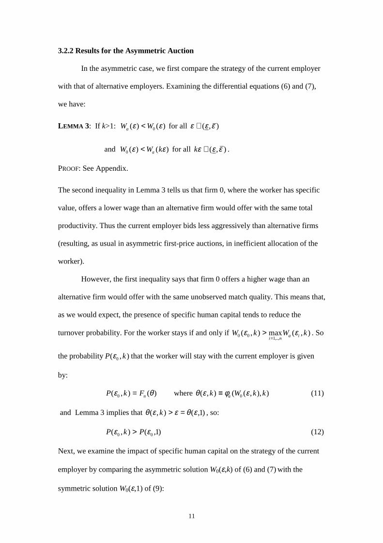
3.2.2 Results for the Asymmetric Auction

In the asymmetric case, we first compare the strategy of the current employer

with that of alternative employers. Examining the differential equations (6) and (7),

we have:

LEMMA 3: If k>1: W Wa ( ) ( )ε ε< 0 for all ε ε ε∈ ( , )

and W W ka0 ( ) ( )ε ε< for all kε ε ε∈ ( , ) .

PROOF: See Appendix.

The second inequality in Lemma 3 tells us that firm 0, where the worker has specific

value, offers a lower wage than an alternative firm would offer with the same total

productivity. Thus the current employer bids less aggressively than alternative firms

(resulting, as usual in asymmetric first-price auctions, in inefficient allocation of the

worker).

However, the first inequality says that firm 0 offers a higher wage than an

alternative firm would offer with the same unobserved match quality. This means that,

as we would expect, the presence of specific human capital tends to reduce the

turnover probability. For the worker stays if and only if W k W ki n

a i0 01

( , ) max ( , ),..,

ε ε>=

. So

the probability P k( , )ε0 that the worker will stay with the current employer is given

by:

P k Fn( , ) ( )ε θ0 = where θ ε φ ε( , ) ( ( , ), )k W k ka≡ 0 (11)

and Lemma 3 implies that θ ε ε θ ε( , ) ( , )k > = 1 , so:

P k P( , ) ( , )ε ε0 0 1> (12)

Next, we examine the impact of specific human capital on the strategy of the current

employer by comparing the asymmetric solution W0(ε,k) of (6) and (7) with the

symmetric solution W0(ε,1) of (9):

12

LEMMA 4 (Sharing of specific human capital): If k>1, W W k kW0 0 01 1( , ) ( , ) ( , )ε ε ε< <

for all ε ≥ ε.

PROOF: See Appendix.

Lemma 4 states that specific human capital raises the wage, but by less than the

increase in productivity. Combined with the result from Lemma 1, w0 =gW0(ε, k), this

implies that the wage determination process has the “classical” properties first

proposed by Becker (1962): the return to general human capital accrues to the worker,

but the return to specific human capital is shared between worker and firm.

4. Derivation of the Earnings Function

Now consider a first-order approximation to ln(w0), the (log) wage offer of the

current employer, valid for k close to 1 (that is, when specific human capital is small

relative to general human capital):

ln ln ( ) ln ln ( , )w g k W0 0 0 0 1≈ + +α ε ε (13)

where α εε

∂∂

( )( , )

≡=

1

10

0

1W

W

k k

From Lemma 4, we have 01

1 110 0

0

<−

−<

W k W

k W

( , ) ( , )

( ) ( , )

ε εε

for k>1 and ε≥ε. Taking the limit

as k tends to 1 gives:

0<α(ε)<1 ∀ ε ε ε∈ [ , ] (14)

Equation (13) is reminiscent of an empirical earnings function, except that the

coefficient on specific human capital is not constant, but varies with the error term.

Intuitively, we might expect this coefficient to decrease as unobserved match quality

ε0 increases. For we know (section 3.2.1) that in the absence of specific capital firms

mark-down the wage more when match quality is high, so it seems plausible that high

13

match quality obviates the need to reward observable specific human capital. Lemma

5 confirms this intuition for the normal and uniform distributions:

LEMMA 5: When unobserved match quality, lnε, has a uniform distribution, or a

symmetric truncated normal distribution, the elasticity of the wage with respect to

observable specific human capital declines with match quality:d

d

αε

< 0 .

PROOF: See Appendix.

Taking expectations of (13) with respect to ε0 gives:

E w g k c[ln ] ln ln0 ≈ + +α (15)

where c W dF= ∫ ln ( , ) ( )0 1ε εε

ε, and α α ε ε

ε

ε= ∈∫ ( ) ( ) ( , )dF 0 1 . Hence:

ln ln lnw g k c0 ≈ + + +α η (16)

where the error term η has expectation zero and is given by:

η ε α ε α≡ − + −(ln ( , ) ) ( ( ) ) lnW c k0 0 01 (17)

Thus we have established:

PROPOSITION 1: A human capital earnings function can be interpreted as a log-linear

approximation to the wage offer function in a labour market auction, valid when

specific human capital is small relative to general human capital. The elasticity of the

wage with respect to general human capital is 1, and the elasticity with respect to

specific human capital lies strictly between 0 and 1.

4.1 Sample Selection Bias

The sample selection problem in estimation of (16) is that a wage offer w0 is

observed only if it is accepted. From (12) we know that (for k close to 1) specific

human capital k increases the probability of acceptance P k( , )ε0 . Unobserved match

quality ε0 also increases this probability, which suggests a negative sample selection

14

bias in estimation of the coefficient on specific human capital: amongst workers who

accept the wage offer of their current firm, those with higher k will have, on average,

lower unobserved match quality than those with low k, and this will obscure the effect

of k on the wage.

To verify this conjecture, we need to examine the expectation of the error term

(17), given acceptance of the wage offer. The density of ε0 conditional on the wage

having been accepted is given by:

!( , )( ) ( )

( ) ( )f k

f F

F dF x

n

n

εε θ

θε

ε=∫

(18)

and:

E W c f k d k f k d[ ] (ln ( , ) ) !( , ) ln ( ( ) ) !( , )η ε ε ε α ε α ε εε

ε

ε

εacceptance = − + −∫ ∫0 1 (19)

The direction of the sample selection bias in the estimation of α is the sign of the

derivative of this expected error with respect to k. Since we are assuming that k is

close to 1, this is given by the sign of:

∂∂

ηε

∂∂

ε α ε α ε εε

ε

ε

ε

k

EW c

f

kd f d

k k

[ ](ln ( , ) )

!( ( ) ) !( , )

acceptance

= =

= − + −∫ ∫1

0

1

1 1 (20)

Thus there are two separate effects leading to sample selection bias. The first

term is shown in Lemma 6(i) below to be unambiguously negative. It represents the

standard sample selection effect discussed above: observed workers with higher

specific human capital have, on average, lower unobserved match quality. The second

term arises because the wage return to specific capital, α, varies with match quality.

If, as was demonstrated in Lemma 5 for the normal and uniform distributions, α

declines as match quality ε increases, then conditioning on acceptance gives more

weight to observations of workers with high ε and low α. So the average reward for

15

specific human capital amongst observed workers is lower than the unconditional

mean and the second term is also negative. Thus we have:

LEMMA 6: (i) (ln ( , ) )!

ε

εε

∂∂

ε∫ − <=

W cf

kd

k

0

1

1 0

(ii) If α(ε) is decreasing in ε, ( ( ) ) ! ( , )ε

εα ε α ε ε∫ − <f d1 0

PROOF: See Appendix.

Now, using Lemmas 5 and 6, we have proved:

PROPOSITION 2: When the distribution of unobserved match quality, lnε, is normal

(with symmetric truncation) or uniform, estimation of the effect on the expected wage

offer of specific human capital, α , is negatively biased due to sample selection.

5. Conclusions

Without specifying the wage determination process we cannot interpret

empirical earnings functions nor resolve the associated problem of sample selection

bias. If wages are predetermined as in the standard model of specific human capital

there is no such bias, but if the earnings function represents a wage offer, we have

demonstrated that there will be a downward bias in the estimated coefficient of

specific human capital in a cross-sectional regression.

The analysis has shown that a wage offer function is an attractive

interpretation of the earnings function, in that it is consistent with earnings functions

as typically estimated, and has the "correct" theoretical properties - in particular the

elasticities with respect to general and specific human capital are as conventionally

assumed.

What does the model tell us about “tenure bias”? If there is a deterministic

functional relationship between tenure and specific human capital then we can apply

16

the results of the model directly, and conclude that if we are estimating a wage offer

function, tenure bias is likely to be negative. Workers with high observable specific

human capital (and tenure) receive a wage premium which makes them more likely to

stay even when unobserved match quality is low, so these workers have, on average,

lower unobserved match quality. This reduces the apparent return to tenure in cross-

sectional data.

If, on the other hand, unobservable shocks to the value of a match can have a

permanent component, it was argued in section 2.2 that this is conceptually equivalent

to specific capital and should be treated as such. Even if the worker and firm did not

intentionally invest in this capital, the problem of finding an appropriate wage to

protect it from loss, once they and competing employers are aware of its existence, is

the same. A period of discovery of permanent match quality might, anyway, be

interpreted as an investment period. In this case, there cannot be a deterministic

relationship between tenure and specific capital, but it is plausible to suppose that

competing employers may use tenure as a signal of its existence.

Since the model is static, is does not allow us to investigate this issue further.

Nevertheless, we can conclude that one of the standard arguments for a positive bias

on the return to tenure – that high tenure merely reflects high match quality – is

misleading. If match quality is permanent, and known to the market, it is effectively

specific human capital; then, if it is not observed by the econometrician we should

expect a negative bias due to measurement error. Temporary, or currently unobserved,

match quality introduces a negative bias.

The other argument for a positive bias is that workers may have an

unobservable characteristic - perhaps "reliability" - that is associated both with higher

productivity and with a tendency to remain in the same job. This is not addressed by

17

the model presented here. We should also note that there are reasons for the inclusion

of tenure that are not related to the existence of specific capital, such as Lazear’s

(1979) shirking story. Again, the model has nothing to say about wages determined

according to incentive considerations.

Finally, we have not considered the inclusion of firm characteristics in the

earnings function. A possible extension of the model would be to allow for an

observable firm specific component of productivity. For the current employer, firm 0,

this would affect wage determination in exactly the same way as specific human

capital – with individual wage determination it does not matter whether this additional

component applies to one worker only or to all employees of the firm. Thus the same

result applies: sample selection will lead to a negative bias. The analysis of the

auction would be considerably more complex, however, if every competing firm had a

different firm specific characteristic. This would introduce asymmetries between all

the players in the wage determination game, and general results would be hard to

obtain – the outcome would depend on the whole vector of firm characteristics.

References

Abraham, K. G. and Farber, H. S. “Job Duration, Seniority and Earnings”. American

Economic Review 77 (June 1987): 278-97.

Altonji, J. G. and Shakotko, R. A. “Do Wages Rise with Job Seniority?”. Review of

Economic Studies 54 (July 1987): 437-59.

Barth, E. “Firm-Specific Seniority and Wages”. Journal of Labor Economics 15 (July

1997): 495-506.

Becker, G. “Investment in Human Capital: A Theoretical Analysis”. Journal of

Political Economy 70 (October 1962): 9-49.

18

Caplin, A. and Nalebuff, B. “Aggregation and Social Choice: A Mean Voter

Theorem”. Econometrica 59 (January 1991): 1, 1-23.

Carmichael, L. “Firm Specific Human Capital and Promotion Ladders”. Bell Journal,

14 (Spring 1983): 251-8.

Gibbons, R. and Waldman, M. “Careers in Organizations: Theory and Evidence”. In

Handbook of Labour Economics, volume 3, edited by O. Ashenfelter and P. R. G.

Layard. Amsterdam: North Holland, 1999.

Hall, R. E. and E. P. Lazear “The Excess Sensitivity of Quits and Layoffs to

Demand”. Journal of Labor Economics 2 (April 1984): 233-57.

Hashimoto, M. “Firm-Specific Human Capital as a Shared Investment”. American

Economic Review 71 (June 1981): 475-82.

Lazear, E. P. “Agency, Earnings Profiles, and Hours Restrictions”. American

Economic Review 71 (September 1981): 606-20.

Maskin, E. and Riley, J. “Equilibrium in Sealed High Bid Auctions”, mimeo,

Department of Economics, Harvard University and University of California, Los

Angeles, 1996a.

Maskin, E. and Riley, J. “Uniqueness in Sealed High Bid Auctions”, mimeo,

Department of Economics, Harvard University and University of California, Los

Angeles, 1996b.

Mincer, J. Schooling, Experience and Earnings, New York: Columbia University

Press, 1974.

Mincer, J. and Jovanovic, B. “Labor Mobility and Wages”. In Studies in Labor

Markets, edited by Rosen, S. (ed) Chicago: University of Chicago Press.

Oi, W. Y. “Labour as a Quasi-Fixed Factor”. Journal of Political Economy 70

(December 1962): 538-55.

19

Stevens, M, “Labour Contracts and Efficiency in On-the-Job Training”. Economic

Journal 104 (March 1994): 408-20.

Topel, R. “Specific Capital, Mobility and Wages: Wages Rise with Job Seniority”.

Journal of Political Economy 99 (February 1991): 145-76.

Appendix

PROOF of (5):

d

d

F

H

F

F

G

Gn

n

n

nεε

= −

∫ ∫sgn

where ( ) ( )Gd

dF F nen n( ) ( ) ( ) ( )ε

εε ε ε ε≡ = +1

= −

∫

F x

F

G x

Gdx

n

n

( )

( )

( )

( )ε εε

ε

( )= − <∫nF x

Ge e x dx

n ( )

( )( ) ( )

εε

ε

ε

0 since by (3) e is decreasing. !

PROOF of LEMMA 3: Subtracting (6) from (7), and writing ef

F( )

( )

( )ε

ε εε

≡ :

e

w

e

w w k wa

a

a

a

( ) ( )φφ

∂φ∂

φφ

∂φ∂ φ φ

0

0

0

0

1 1− =

−−

− (A1)

First consider y w a( ) ≡ −φ φ0 . If y=0 at w w w0 ∈ ( , ] , (A1)⇒ dy

dw> 0 . But y=0 at w .

Hence there can be no other such w0 , and y w( ) < 0 ∀ w< w .

Now let z w ka( ) ≡ −φ φ0 . If z=0 at w w w0 ∈ ( , ) , (A1)⇒ ew

e kk w

a( ) ( )φ∂φ∂

φ∂φ∂0

00

10− = .

And from (3), e k e( ) ( )φ φ0 0< , so at w0 , dz

w∂> 0 . But z w< 0 at . Hence there can be

no such w0 , and z w( ) < 0 ∀ w≤ w .

20

Thus we have established that φ φ φ0 0( ) ( ) ( )w w k wa< < for all w w w∈ ( , ) ; inverting

gives the required inequalities for the wage offer functions. !

PROOF of LEMMA 4: Subtracting (9) from (6), and using Lemma 3:

e

w

e

w k w w w wa

a

a

a

( ) ( )φφ

∂φ∂

φφ

∂φ∂ φ φ φ φ

− − =−

−−

<−

−−

1 1 1 1

0

(A2)

We will prove the inverse inequality:φ φ φ0 0( ) ( ) ( )w w kw< < for all w≥w.

For the lower inequality, let y w a( ) ≡ −φ φ. At w(k) (>ε), from (8), y<0. If y=0 at

w w w0 ∈ ( , ] , (A2)⇒ dy

dw< 0 . Hence there is no such w0 , and φ φa < ∀ w< w . From

Lemma 3, φ φ0 < ∀ w< w .

For the upper inequality, let ψ φ≡ ( / )w k . (9) can be written: e

w n k w

( )ψψ

∂ψ∂ ψ

=−

1 1.

Also, from (6) and (7): e

w w

n

n k wa

( )φφ

∂φ∂ φ φ

0

0

0

0

1 1 1=

−−

−−

. Subtracting:

e

w

e

w w k w n k w k wa

( ) ( )φφ

∂φ∂

ψψ

∂ψ∂ φ φ φ ψ

0

0

0

0 0

1 1 1 1 1− =

−−

−

+

−−

−

(A3)

Consider z w( ) ≡ −φ ψ0 . When w=kε, from (8), z>0.

If z=0 at w k0 > ε , (A3)⇒ dz

dw> 0 . Hence there is no such w0 , and z>0 ∀ w k> ε , or

equivalently φ φ( ) ( )w kw< 0 for all w≥ε. This establishes the inequalities forφ φ0 and ;

inverting gives the inequalities for the wage offer functions. !

PROOF of LEMMA 5: Transform equations (6) and (7), putting w W k= 0 ( , )ε and

θ ε φ ε( , ) ( ( , ), )k W k ka≡ 0 as in (11):

ne

k WW( )

( )θθ

∂θ∂ε

ε∂∂ε

− =00 (6’)

21

( )( ) ( )

( )ne e

WW

− +

− =1 00θ

θ∂θ∂ε

εε

θ∂∂ε

(7’)

Differentiating (6’) and (7’) with respect to k, setting k=1, and rearranging:

∂∂ε∂

ε∂∂ε

εε

∂θ∂

εε

ε∂∂

20

00W

kn W

e

kn

e W

k= −

+ −

( )

( ) ( )

0 00= −

+ −

( )

( ) ( )ε

∂∂ε

εε

∂θ∂

εε

ε∂∂

We

kn

e W

k

Now, when k=1, ε ε ε− =W H Fn n0 ( ) / ( ) (equation 6), and α εε

∂∂

( )( , )

≡=

1

10

0

1W

W

k k

.

Define similarly β εε

∂θ∂

( ) ≡=

1

1k k

. We can transform these equations to obtain a pair of

differential equations in α and β:

′ +′

+ − =β β βe

e

nF

Hn

n

( )1 0 (A4)

( )′ =−

− − −α

εα β

ne

H Fn

n n/( )1 1 (A5)

We already know that 0<α<1. From Lemma 3 ε θ ε< < k , so 0<β<1.

At ε, α βε

= ==

1

1

d w

dkk

. From Lemma 2(i) w satisfies nf w

F wk w

( )

( )( )ε − = 1, from

which we obtain:

1

1

2

2εd w

dk

nf w

n f w F w f w=

+ − ′( )

( ) ( ) ( ) ( )

When k=1, w=ε ; hence α ε β ε( ) ( )= =+n

n 1.

Consider equation (A4). This can be written:

′ = − −′

+ +

−β

εβ

1 f

f

f

F

nF

H

nF

Hn

n

n

n

22

The bracketed term is positive (by (3)); so when β ≤+n

n 1:

′ ≤+

− −′

+ −

<

+− −

′− −

β

ε εn

n

f

f

f

F

F

H

n

n

f

fn

f

Fn

n1

1

1

11( )

(using the log-concavity of Hn).

When lnε has a uniform distribution, 1

0ε

+′

=f

f, and ′β is negative whenever

β ≤+n

n 1. Since β ε( ) =

+n

n 1, this means that ′β is negative for all ε.

When lnε is truncated normal4, 1

εε

ε+

′= −

f

f

ln, so by the same argument ′β is

negative for all ε≤1. Now suppose ′ =β 0 at some1 0< <ε ε .

Differentiating (A4) ⇒ ′′ = −′

β

∂∂ε

ε εε ε

sgn ( )

( )

e

e

H

Fn

n

at ε0 .

Hn/ε Fn is positive and increasing, and, by Lemma A1, so is −′

ε e

efor the normal

distribution when ε≥1. So ′′ >β 0 at ε0 . But this is impossible because at

ε θ ε ε, ( ) , = ∀ k so β=0, and ′ <β 0 . Hence ′ <β 0 ∀ ε.

Now consider equation (A5).

At ε, α β= ⇒ ′ <α 0 . Differentiating shows that if ′ =α 0 at some ε ε0 > ,

′′ = ′ <α βsgn

0 . This is impossible, so ′ <α 0 ∀ ε. !

LEMMA A1: When lnε has a symmetric truncated normal distribution,

d

d e

de

dεε

ε−

> 0 for all ε>1.

23

PROOF: ef

F

g

G( )

( )

( )

(ln )

(ln )ε

ε εε

εε

≡ = where g xc

x( ) exp( / )= −2

22

π for some constant c

and G is the corresponding distribution function.

It is sufficient to prove that y xd

dx

g x

G x( )

ln ( )

( )≡

2

2 <0 for x>0.

Evaluating this: yg

Gx

g

G= +

− 1. When x=0, symmetric truncation ⇒ G=½, and it

can be verified that y<0. Then:

dy

dxy x

g

G

g

Gy= − + +

−( )1

so if y=0 at any x0>0, dy/dx<0. Hence there can be such x0, and y<0 ∀ x>0. !

PROOF of LEMMA 6: (i) ( )∂∂

θ ε∂θ∂

ε ε β εk

F fk

nF enk

nk

n( ) ( ) ( ) ( ) ( )= =

= =1 1

where β is

defined as in the proof of Lemma 5. Hence:

∂∂

ε ε ε β ε β ε ε

ε

ε

ε

ε

ε

ε

ε

! ( ) ( ) ( ) ( ) ( ) ( ) ( ) ( ) ( ) ( ) ( ) ( )

( ) ( )

f

kn

F x dF x f F e F x e x x dF x f F

F dF xk

n n n n

n=

=

−

∫ ∫

∫1

2

and it is required to prove that:

F dF W c F e dF

F e dF W c F dF

n n

n n

( ) ( ) (ln ( , ) ) ( ) ( ) ( ) ( )

( ) ( ) ( ) ( ) (ln ( , ) ) ( ) ( )

ε ε ε ε ε β ε ε

ε ε β ε ε ε ε ε

ε

ε

ε

ε

ε

ε

ε

ε

∫ ∫

∫∫

−

< −

0

0

1

1

or equivalently, since F f f nn n( ) ( ) ( ) / ( )ε ε ε= ++1 1 :

(ln ( , ) ) ( ) ( ) ( ) ( ) ( ) ( ) (ln ( , ) ) ( )W c e dF e dF W c dFn n n0 1 1 0 11 1ε ε β ε ε ε β ε ε ε εε

ε

ε

ε

ε

ε− < −∫ ∫∫+ + +

We know that lnW0 is an increasing function of ε, and from equation (A4) eβ is a

decreasing function of ε. Hence by Lemma A2 below this inequality holds.

! ( , )( ) ( )

( ) ( )f k

f F

F dF x

n

n

εε θ

θε

ε=∫

24

(ii) ( ( ) ) ! ( , ) ( ( ) ) ( ) ( )sgn

ε

ε

ε

εα ε α ε ε α ε α ε ε∫ ∫− = −f d F dFn1

< −∫ ∫( ( ) ) ( ) ( ) ( )ε

ε

ε

εα ε α ε ε εdF F dFn by Lemma A2

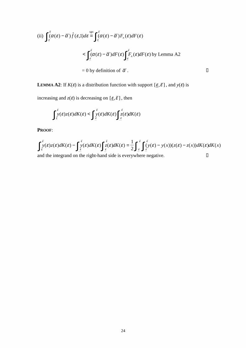
= 0 by definition of α . !

LEMMA A2: If K(ε) is a distribution function with support [ , ]ε ε , and y(ε) is

increasing and z(ε) is decreasing on [ , ]ε ε , then

y z dK y dK z dKε

ε

ε

ε

ε

εε ε ε ε ε ε ε∫ ∫ ∫<( ) ( ) ( ) ( ) ( ) ( ) ( )

PROOF:

y z dK y dK z dK y y x z z x dK dK xε

ε

ε

ε

ε

ε

ε

ε

ε

εε ε ε ε ε ε ε ε ε ε∫ ∫ ∫ ∫∫− = − −( ) ( ) ( ) ( ) ( ) ( ) ( ) ( ( ) ( ))( ( ) ( )) ( ) ( )

1

2

and the integrand on the right-hand side is everywhere negative. !

25

Footnotes

1 Barth (1997), using a Norwegian dataset that enabled him to control for firm

heterogeneity, also found a significant positive tenure effect.

2More precisely, the shock to internal productivity must be distributed identically to

the negative of the shock to the opportunity wage.

3This is a model of wage determination for a worker already possessing some specific

and some general human capital; we do not model the investment process, and the

sharing of costs. However, it would be straightforward to do so: the incentives for the

worker and firm to invest can be determined by calculating their expected returns.

4 This proof is for the standard normal with mean zero and unit variance; it extends to

the general case in the obvious way.