reconfigurable bioimpedance spectrometer for the...

Reconfigurable Bioimpedance Spectrometer for the

Evaluation of Impedance Estimation Methods Suitable

for Spectroscopy Measurements Master of Science Thesis in Biomedical Engineering

ZELEALEM KEBKAB KASSAYE

Department of Signals and Systems

Division of Biomedical Engineering

CHALMERS UNIVERSITY OF TECHNOLOGY

Göteborg, Sweden, 2012

Report No. 033/2012

i

Reconfigurable Bioimpedance Spectrometer for the

Evaluation of Impedance Estimation Methods Suitable

for Spectroscopy Measurements

ZELEALEM KEBKAB KASSAYE

Department of Signals and Systems

Division of Biomedical Engineering

CHALMERS UNIVERSITY OF TECHNOLOGY

Telephone +46(0)735744054

Supervisor: Fernando Seoane University of Borås School of Engineering SE-501 90 Borås Sweden Telephone +46(0) 334354008

Examiner: Bo Håkansson Chalmers University of Technology SE-412 96 Göteborg Sweden

Telephone +46(0) 317721807

ii

Dedicated to

Our late mother Ejigayehu Mekuria

iii

Abstract

The measurement of electrical bioimpedance deals with the measurement of the opposition to the

flow of charges exhibited by a biological material when an electrical stimulus is applied. The

impedance estimation implemented in an impedance meter is a paramount key functional blocks

influencing in the measurement performance and application of the measurement device. In this

work a configurable bioimpedance measurement system has been implemented using the NI

USB-6218 Data Acquisition board and LabVIEW development environment. The implemented

system allows the implementation of different impedance estimation methods and tests their

performance. To show the intended functionality two different impedance estimation methods

have been implemented: Digital Sine Correlation and Digital Deconvolution through Total Least

Squares. The performances of both systems have been validated with 2R1C circuits. The

multisine excitation implemented with two NI USB-6218 units produce a time delay that

required signal synchronization prior the application of digital deconvolution. The measurement

results show that is possible to produce multifrequency bioimpedance measurements with both

approaches well using frequency sweeping or multisine excitation.

Key words: Electrical bioimpedance Spectroscopy, Total Least Square, Digital Sine Correlation,

Digital Deconvolution NI USB-6218 Data Acquisition Device, LabVIEW.

iv

Acknowledgments

Thanks to the Almighty for giving me the strength and courage to do all the things.

The successful completion of this work is unthinkable without the help of my supervisor

Fernando Seoane. His continued guidance, support, encouragement and patience made me to

reach the point of accomplishing this work. I greatly appreciate him for everything he put on me.

I also appreciate my examiner Bo Håkansson for giving his time for my thesis work.

I appreciate and thank all my family members here in Sweden and back home in Ethiopia

Kebkab, Tewodros, Adane and Kerima for their unconditional support, encouragement during all

my study years and especially during this thesis work. I also want thank my classmates for their

help and support during my study and stay here.

Last but not least I want to thank Tefera Tafesse, Per Olcén, Anders Bergström and many others

for their kind support during my study.

Zelealem Kebkab Kassaye

25th May 2012

Göteborg, Sweden

v

List of Figures

Figure 2-1 Complex Representation of Impedance. ....................................................................... 4

Figure 2-2 Structure of a cell with Intra- and Extracellular Fluid, plasma membrane Nucleus and its Equivalent Electrical Circuit. ..................................................................................................... 6

Figure 2-3 Injected Current Path at (a) Low Frequency and (b) High Frequency in Biological Tissues............................................................................................................................................. 8

Figure 2-4 Regions of Dispersion, Frequency verses Permittivity and Conductivity. ................... 9

Figure 2-5 Bioimpedance Measurements system (a) Two Electrode Setup and (b) Its Equivalent Electrical Circuit. .......................................................................................................................... 10

Figure 2-6 Bioimpedance Measurements system (a) Four Electrode Setup and (b) its Equivalent Electrical Circuit. .......................................................................................................................... 11

Figure 3-1 Block Diagram of Components and their connections. .............................................. 12

Figure 3-2 Load-in-the-Loop Single Operational Amplifier Voltage Controlled Current Source........................................................................................................................................................ 14

Figure 3-3 Practical Single Operational Amplifier Voltage Controlled Current Source Design. 15

Figure 3-4 NI USB-6218. ............................................................................................................ 16

Figure 3-5 Grounded Signal Source. ............................................................................................ 17

Figure 3-6 Floating Signal Source. ............................................................................................... 17

Figure 3-7 Differential Mode Measurement Setup. ...................................................................... 18

Figure 3-8 Referenced Single-Ended Mode Measurement Setup. ................................................ 18

Figure 3-9 Non-Referenced Single-Ended Mode (NRSE) Measurement Setup. ......................... 19

Figure 3-10 Digital Sine Correlation Estimation Method Block Diagram. .................................. 20

Figure 3-11 Digital Sine Correlation LabVIEW Implementation. ............................................... 23

Figure 3-12 Measurement Setup for EBI Estimation Using TLS with In-Phase (Sin (ωt)), In-Quadrature (Cos (ωt)) and Measurement Voltage Vm. ................................................................. 25

Figure 3-13 Multifrequency EBI Measurement System Implementation –Total Least Square Method. ......................................................................................................................................... 33

Figure 3-14 Multifrequency EBI Measurement System VCCS. .................................................. 34

Figure 3-15 Plot showing the four reference voltages at frequencies 300, 1400, 2500 and 3600 Hz and the measurement voltage before synchronization with their corresponding phase shifts at the right side of the plot. ............................................................................................................... 35

Figure 3-16 Plot showing the four reference voltages at frequencies 1000, 2000, 3000 and 4000 Hz and the measurement voltage after synchronization with their corresponding phase shift at the right side of the plot. ..................................................................................................................... 36

Figure 3-17 Plot showing the four reference voltages at frequencies 1000, 2000, 3000 and 4000 Hz and the measurement voltage after synchronization and time delay removal at the first and third measurement frequency with their corresponding phase shift at the right. .......................... 37

Figure 4-1 GUI of the Single Frequency Measurement system. .................................................. 39

Figure 4-2 Schematic Showing the measurement Setup with the (inset) 2R1C Equivalent Electrical Circuit with Components. ............................................................................................. 39

Figure 4-3 Single Frequency-Plot of Frequency versus Resistance Measurement, Theoretical and Calibrated values of 20nF 2R1C parallel model. .......................................................................... 42

Figure 4-4 Single Frequency-Plot of Frequency versus Reactance Measurement, Theoretical and Calibrated values of 20nF 2R1C parallel model. .......................................................................... 42

Figure 4-5 Single Frequency-Plot of Resistance versus Reactance Measurement, Theoretical and Calibrated values of 20nF 2R1C parallel model. .......................................................................... 43

vi

Figure 4-6 Single Frequency-Plot of Frequency versus Resistance Measurement, Theoretical and Calibrated values of 40nF 2R1C parallel model. .......................................................................... 46

Figure 4-7 Single Frequency-Plot of Frequency versus Reactance Measurement, Theoretical and Calibrated values of 40nF 2R1C parallel model. .......................................................................... 46

Figure 4-8 Single Frequency-Plot of Resistance versus Reactance Measurement, Theoretical and Calibrated values of 40nF 2R1C parallel model. .......................................................................... 47

Figure 4-9 GUI of the Multifrequency Measurement system. ...................................................... 48

Figure 4-10 Voltage Controlled Current Source with the 2R1C Parallel Model in Multifrequency Impedance Measurment. ............................................................................................................... 49

Figure 4-11 Plot of Frequency versus Resistance Measurement, Theoretical and Calibrated values of 2R1C circuit with 20nF. ................................................................................................ 53

Figure 4-12 Plot of Frequency versus Reactance Measurement, Theoretical and Calibrated values of 2R1C circuit with 20nF. ........................................................................................................... 53

Figure 4-13 Plot of Resistance versus Reactance Measurement, Theoretical and Calibrated values of 2R1C circuit with 20nF. ........................................................................................................... 54

Figure 4-14 Plot of Frequency versus Resistance Measurement, Theoretical and Calibrated values of 2R1C circuit with 40nF. ................................................................................................ 55

Figure 4-15 Plot of Frequency versus Reactance Measurement, Theoretical and Calibrated values of 2R1C circuit with 40nF. ........................................................................................................... 56

Figure 4-16 Plot of Resistance versus Reactance Measurement, Theoretical and Calibrated values of 2R1C circuit with 40nF. ........................................................................................................... 56

vii

List of Tables

Table 2-1 Electrolyte and protein anion concentration (Gerard J. Tortora 2007). ......................... 5

Table 4-1 Single Frequency-Resistive Part Estimated, Theoretical and Calibrated values of 20nF 2R1C Circuit. ................................................................................................................................ 40

Table 4-2 Single Frequency-Reactive Part Estimated, Theoretical and Calibrated values of 20nF 2R1C Circuit. ................................................................................................................................ 41

Table 4-3 Single Frequency-Resistive Part values, Theoretical and Calibrated, for 2R1C Circuit with 40nF. ..................................................................................................................................... 44

Table 4-4 Single Frequency- Reactive Part values, Theoretical and Calibrated for 2R1C Circuit with 40nF. ..................................................................................................................................... 45

Table 4-5 Measurement Mean Absolute Errors (MAE) and Standard Deviation (STD) of Two DAQs measurement setup at Sampling Frequency of 80kHz. ..................................................... 50

Table 4-6 Measurement Mean Absolute Errors (MAE) and Standard Deviation (STD) for one DAQ measurement setup at Sampling Frequency 50 kHz .......................................................... 51

Table 4-7 Resistive Part Estimated, Theoretical and Calibrated values for 2R1C Circuit with 20nF. ............................................................................................................................................. 52

Table 4-8 Reactive Part Estimated, Theoretical and Calibrated values for 2R1C Circuit with 20nF. ............................................................................................................................................. 52

Table 4-9 Resistive Part Estimated, Theoretical and Calibrated values for 2R1C Circuit with 40nF. ............................................................................................................................................. 54

Table 4-10 Reactive Part Estimated, Theoretical and Calibrated values for 2R1C Circuit with 40nF. ............................................................................................................................................. 54

viii

List of Acronyms

AC Alternating current

DAQ Data Acquisition

DC Direct Current

DSC Digital Sine Correlation

EBI Electrical Bioimpedance

EBS Electrical Bioimpedance Spectroscopy

ECW Extracellular Water

FFT Fast Fourier Transform

ICW Intracellular Water

LabVIEW Laboratory Virtual Instrument Engineering Workbench

LS Least Square

NI National Instruments

PFI Programmable Function Interface

SVD Singular Value Decomposition

TLS Total Least Square

VCCS Voltage Controlled Current Source

Z Impedance

ix

Table of Contents

Abstract ...................................................................................................................................... iii Acknowledgments ...................................................................................................................... iv

List of Figures ............................................................................................................................. v

List of Tables ............................................................................................................................. vii List of Acronyms ...................................................................................................................... viii Table of Contents ....................................................................................................................... ix

Chapter 1. Introduction ........................................................................................................... 1

1.1 Introduction ..................................................................................................................... 1

1.2 Motivation ....................................................................................................................... 1

1.3 Goal ................................................................................................................................. 2

1.4 Work done ....................................................................................................................... 2

1.5 Structure of the Report .................................................................................................... 2

1.6 Out of Scope ................................................................................................................... 3

Chapter 2. Background-Bioimpedance .................................................................................. 4

2.1 Introduction to Bioimpedance......................................................................................... 4

2.2 Electrical Properties of Biological Tissues ..................................................................... 5

2.2.1 Plasma Membrane ....................................................................................................... 5

2.3 Equivalent Electrical Circuit of a Cell ............................................................................ 6

2.4 Dispersion of a Biological Tissue-Frequency Dependency ............................................ 8

2.5 Bioimpedance Measurement ........................................................................................... 9

2.5.1 Electrode Arrangement ............................................................................................. 10

2.5.1.1 Two Electrodes System ............................................................................... 10

2.5.1.2 Four Electrodes System .............................................................................. 10

Chapter 3. Materials and Methods ....................................................................................... 12

3.1 Materials and Methods .................................................................................................. 12

3.2 Current Source .............................................................................................................. 12

3.2.1 Voltage Controlled Current source (VCCS) ............................................................. 13

3.2.1.1 Load-in-the-Loop ........................................................................................ 13

3.2.1.2 Practical Load-in-the-loop VCCS Design................................................... 14

3.3 Data Acquisition and Analysis Hardware ..................................................................... 15

3.3.1 National Instruments NI USB-6218.......................................................................... 15

3.3.2 Merits and Limitations of NI USB-6218 .................................................................. 16

3.4 Measurement Systems .................................................................................................. 16

3.4.1 Signal Sources ........................................................................................................... 16

3.4.1.1 Grounded Signal Sources ............................................................................ 16

3.4.1.2 Floating Signal Sources .............................................................................. 17

3.4.2 Measurement Systems Modes................................................................................... 17

3.4.2.1 Differential Mode ........................................................................................ 17

3.4.2.2 Referenced Single-Ended Mode (RSE) ...................................................... 18

3.4.2.3 Non-Referenced Single-Ended Mode (NRSE) ........................................... 18

3.5 Laboratory Virtual Instrument Engineering Workbench (LabVIEW™) ...................... 19

3.6 Impedance Estimation Methods .................................................................................... 19

3.6.1 Single Frequency measurement Estimator ................................................................ 20

3.6.1.1 Digital Sine Correlation (DSC) ................................................................... 20

x

3.6.2 Multifrequency Bioimpedance Measurement Estimators ......................................... 24

3.6.2.1 Total Least Square (TLS) Method .............................................................. 24

3.6.2.2 Synchronization of the DAQs ..................................................................... 35

Chapter 4. Results .................................................................................................................. 38

4.1 Measurement Results .................................................................................................... 38

4.2 Single Frequency Measurement .................................................................................... 38

4.2.1 Single Frequency Measurement System GUI ........................................................... 38

4.2.2 Single Frequency Measurement Results ................................................................... 39

4.3 Multifrequency Measurement ....................................................................................... 47

4.3.1 Multifrequency Measurement System GUI .............................................................. 47

4.3.2 Multifrequency Measurement Results ...................................................................... 48

Chapter 5. Discussion............................................................................................................. 57

Chapter 6. Conclusion and Future Work ............................................................................ 59

6.1 Conclusion .................................................................................................................... 59

6.2 Future work ................................................................................................................... 59

References .................................................................................................................................... 60

Appendix ...................................................................................................................................... 62

Appendix A.1 NI USB-6218 Specification Summary * ........................................................... 62

Appendix A.2 NI USB-6218 Pinout * .................................................................................... 64

1

Chapter 1. Introduction

1.1 Introduction

The opposition experienced when an electrical charges flow through a biological material is

known as Electrical Bioimpedance (EBI). These biological materials do not only exhibit an

opposition to the flow of electrical charges but can store electrical energy, the charges and field

also experience a phase shift. Therefore, EBI measurements must be represented as a complex

number.

The measurement of EBI is a relatively simple and requires two or more electrodes. The

measurement can be use to asses in the subject’s blood flow, cardiac activity, respiration activity,

bladder, blood and kidney volumes and etc (Sverre Grimnes 2006). When the EBI measurements

are taken at various frequency points it is called EBI spectroscopy. Measuring the impedance in a

range of frequencies gives a spectrum that can easily show the relationship between impedance

and frequency. This relationship can give an indication about the status of the biological tissue

under study (Zilico 2012). The applications of the measurements of EBI spectroscopy include the

assessment of intracellular water (ICW) and extracellular water (ECW) conditions (M.Tengvall

2009).Therefore several applications can be built up based on performance of EBI measurements

and it is a non-invasive method of measurement of physiological conditions.

1.2 Motivation

For trained technician, a measurement of an EBI is a forward task to perform and it is non-

invasive. Even if EBI spectroscopy is simple to perform its measurement performance and

applications are dependent on the different functional building units of it. The impedance

estimation block is one of the main functional blocks of EBI spectroscopy. The others include

electrodes, voltage and current measurement blocks. The study of the building blocks of EBI

measurement systems and setups is helpful in having a good quality measurement result.

Constructing EBI measurement setup that can be configurable is a need to study the influence

that each of the building blocks creating to the measurement results. Designing an analog current

source and using LabVIEW development environment and NI USB-6218 multifunction data

acquisition card (DAQ) allow to study how the building blocks mainly the impedance estimation

block is affecting the overall measurement result. The impedance estimation block can easily be

configured as the study’s need in such custom made EBI spectrometer. Its effect on the

measurement results can be shown by doing different configuration at different setups like

number of sample used in the estimation and the use of different voltage or current measurement

configuration.NI USB-6218 is USB powered device hence can be driven by portable computer

battery power. This enhances the electrical safety regarding applications on human beings.

2

1.3 Goal

The goal of this work is to implement a bioimpedance spectroscopy meter that can work at a

single and multi-frequency that allows test the performance and influence on the measurements

of different alternatives to the functional blocks and especially for different impedance

estimation approaches. Commercially available meters are made application specific and do not

allow modifying them and sometimes making impossible to use in experimental environments.

There are different impedance estimation approaches; some of them are Digital Sine Correlation

(DSC), Digital Deconvolution by Total Least Square (TLS) and Fast Fourier Transform (FFT)

methods. The performance comparison of the two EBI measurement estimation approaches,

DSC of frequency sweeping application and digital convolution by TLS of multifrequency

application is used to evaluate the correct operation of the implemented EBI spectroscopy meter.

1.4 Work done

In this thesis the executed work includes design and analog electronic implementation of a

Voltage Controlled Current Source (VCCS), implementation of DSC using LabVIEW and

measurement of an equivalent electrical circuit of cells using 2R1C parallel model. Calibration is

done on a known set of 2R1C parallel model. Measurements are taken with different sets of

2R1C parallel model using the calibrated setup. The raw measurements, theoretical values and

calibrated measurements of a 2R1C parallel model given as result of this work.

The multifrequency estimation of bioimpedance is implemented using the TLS method and used

Singular Value Decomposition (SVD) as a computational tool. An analog circuit of summing

amplifier in an inverted operational amplifier configuration is used as a VCCS and TLS is

implemented using the LabVIEW on NI USB-6218 DAQ card. The raw measurements,

theoretical values and the calibrated measurements of a 2R1C parallel model given as a result of

this work.

1.5 Structure of the Report

The sections that are contained in this thesis report are six chapters, a bibliography and an

appendix section. Chapter one Introduction contains the introduction, motivation, goal and work

done on this thesis. Additionally parts that are not covered on this work are listed in out of scope

part of this chapter. Chapter two of this work, Background-Bioimpedance discusses about the

basic concepts of electrical bioimpdance, the electrical properties of biological a tissues,

equivalent electrical circuit of a cell and bioimpedance measurement systems including electrode

configuration. Chapter three, Methods and Materials, covers the methods and materials used in

measurement of EBI with their implementation in this work. Current source types, data

acquisition and analysis hardware and the measurement setup are the other things that are

discussed in chapter three. Chapter four Results, contains the EBI measurement results that are

taken during this work. Chapter five Discussion, discuses the EBI measurement results of the

work. The last chapter ,Chapter six Conclusion and Future work, puts the conclusion that is

drawn from the work and gives the possible further extensions of this work.

3

In the Appendix section of this work, the bibliography used and the specification summary of the

DAQ are given.

1.6 Out of Scope

In this work the following points are not studied

• To test the performance of the implemented EBI spectrometer in human subjects is not included.

• Comparisons of different measurement parameters that affect the impedance estimation are not studied.

• Any comparison of the obtained measurement performance with commercially available devices is not studied.

4

Chapter 2. Background-Bioimpedance

2.1 Introduction to Bioimpedance

The electric impedance is an opposition that a material present when excited by an electrical

stimulus like alternating current (AC) of particular frequency. The electrical impedance (Z) is

given by a complex relation that has two components, the first real part is denoted by R which is

resistive component of the impedance and the imaginary part is denoted by X which is the

reactive component of the impedance and shown as follows

= + [Ω]

= ||∠

Where || = √ + = tan

= ||cos and = || sin Equation 2.1

This can be given in a graphical representation in a complex plane as below.

Figure 2-1 Complex Representation of Impedance.

5

As a material, biological tissues have different types of properties that include their electrical

behavior. EBI is one of its electrical properties (Tabuenca 2009). EBI is the resistance that is

created when a biological tissue is subjected to an electrical excitation of current or voltage and it

is dependent on the value of the frequency of excitation of the current or voltage. The

measurement of EBI to assess and study the behavior of the biological tissues as it is subjected to

an AC has a long lasting history (Patterson 2000).

2.2 Electrical Properties of Biological Tissues

A biological tissue is made up of cells that perform a particular function in the organism’s body.

The cells building these tissues are suspended on a fluid called extracellular (outside cell) fluid.

It is composed mainly of interstitial (between cells) fluid (about 80%) and the remaining part is

composed of blood plasma (about 20%), a liquid part of the blood. The cells also have fluid

inside them - intracellular (inside cell) fluid or cytosol of the cell in which the organelles of the

cell are suspended. In these fluids electrolytes like Na+, K+, Cl-, Ca2+ and proteins occur. These

electrolytes are free to move in the fluids that they are predominantly found and as well to the

other fluid. The concentration and presence of each of the electrolytes in the extracellular fluid is

different from that of the intracellular fluid (Gerard J. Tortora 2007).

Table 2-1 Electrolyte and protein anion concentration (Gerard J. Tortora 2007).

Electrolyte/protein anion

Concentration(mEq/lit)

Extracellular fluid

Intracellular fluid

Na+ 142 10

K+ 4 140

Cl- 100 3

Ca2+

5 0.2

Protein anions 20 50

Unlike metal conductors, the free moving ions in both fluids are serving as charge carriers which

in turn are responsible in creating the electrical conductive property of biological tissues.

2.2.1 Plasma Membrane

Plasma membrane is a life line of the cell; if it is destroyed a cell will die. Plasma membrane

encloses the cell and it makes a compartment for the extracellular fluid and intracellular fluid.

The plasma membrane is built from phospholipids- lipids that have phosphors. It is constructed

in such a way that the two phospholipids layers come into back to back forming a lipid bilayer

(Gerard J. Tortora 2007). The plasma membrane has a resistivity of approximately 100Ω/cm2 and

1µF/cm2 of capacitance per unit area and shows a property of a capacitor which varies as the

value of the frequency of the excitation AC changes. The intracellular fluid which is an ionic

solution has around100Ω/cm and extracellular fluid has approximately 60Ω/cm (Tabuenca 2009).

6

2.3 Equivalent Electrical Circuit of a Cell

Biological tissues are formed from a number of cells that have the same type of function in the

organism’s body. Its properties are derived from the cumulative properties of the cells that are

the building block of the biological tissue. Having an equivalent electrical circuitry

representation of a Cell is basic tool in studying their electrical property especially their

Bioimpedance property (Seoane 2007). This equivalent electrical circuitry has a simple

representation of the extracellular fluid, intracellular fluid and the plasma membrane with a

combination of resistors and capacitors.

A simple way of giving the equivalent electrical circuitry model is called Fricke’s circuit. The

Fricke’s circuit put the circuit model of cells as the two fluids in the biological tissue i.e.

extracellular and intracellular fluids, in parallel and the barrier between them i.e. the plasma

membrane as a capacitor which is in series with the intracellular fluid (Ursula G. Kyle 2004).

Figure 2-2 Structure of a cell with Intra- and Extracellular Fluid, plasma membrane Nucleus and its

Equivalent Electrical Circuit.

The equivalent impedance of the model is calculated easily from the given components Re, Ri,

and the impedance value of the capacitor is given by Xc and is equal to:

= − 12"#$ [Ω]

Equation 2.2

Then Ri and Xc are in series and they become

% + =% + 12"#$

Equation 2.3

7

and on the other electrical branch of the model Re is in parallel with Equation 2.3. This gives the equivalent impedance of the model as follows

= &||'% + ( = & × '% + 12"#$(& +'% + 12"#$(

= & × '% × 2"#$ + 1(2"#$'& × 2"#$ + % × 2"#$ + 1(2"#$

= & × % × 2"#$ + &'& × 2"#$ + % × 2"#$ + 1(

= & × '1 +% × 2"#$(2"#$'& + %( + 1

Rearranging and substituting Equation 2.4 into the above equation

* = 2"#

Equation 2.4

is resulting the equivalent impedance of the simple cell model for biological tissues. The final equation is given by

= &'1 + %*$(1 + *$'& + %( Equation 2.5

Equation 2.5 is able to show the behavior of the equivalent impedance at low or zero frequency and at high or infinite frequency. At lower frequency (ω = 0), the plasma membrane hinders the excitation AC from passing through it and it makes its way across the extracellular fluid outside of the cells. This results the equivalent impedance to become (Ursula G. Kyle 2004).

+ =&

At higher frequencies (ω = ∞), the plasma membrane that is given by Cm in the model behaves as a perfect conductor and its impedance which is given in Equation 2.2 is becomes zero and the respective equivalent impedance becomes a parallel combination of the Re and Ri which is the combination of the extracellular and intracellular fluids and is given as below (Ursula G. Kyle 2004).

8

, =& × %& + %

The above phenomenon is illustrated in the following figure that is showing how low frequency and high frequency signals interact with cells and fluids inside and outside of them.

Figure 2-3 Injected Current Path at (a) Low Frequency and (b) High Frequency in Biological Tissues.

2.4 Dispersion of a Biological Tissue-Frequency Dependency

When the permittivity of material changes as a function of the frequency of the exciting stimulus, the material is called dispersive medium. Biological tissues show this behavior and can put under this category of materials (Seoane 2007). As frequency of the excitation AC increases, the permittivity of the biological tissue shows a decrease where as conductivity increases. There are windows of dispersion that were revealed and given the names α, β, γ- dispersion by H.P. Schwan (1963). These windows can be seen when plotting the spectrum of permittivity or conductivity of biological tissues.

9

Figure 2-4 Regions of Dispersion, Frequency verses Permittivity and Conductivity.

The α – dispersion is present in a frequency range of mHz to kHz. In the range of 1 kHz to 100MHz, the β – dispersion is the predominant dispersion. The range 0.1 GHz to 100 GHz is dedicated to the γ – dispersion (Sverre Grimnes 2008). But it is not possible to exactly demarcate each windows as they are continues one into the other window (P.Schwan 2001).

2.5 Bioimpedance Measurement

Measurement of the impedance Z of a given tissue can be performed using two different approaches. Applying a controlled amount of AC current to the tissue and measuring the response AC voltage is the first approach and the most common way of measurement (R. Gordon 2005).The second methodology is done by applying AC Voltage to the tissue and measuring the response AC current.

At the first approach the excitation AC current I and the response AC voltage are known from the measurement setup. The excitation AC voltage V and the response AC current are known in the second approach. From both the approaches the known values are enough to derive the complex impedance of the tissue by applying the Ohm’s law. The Ohm’s law is given by:

= -. [/] Where Z = R + jX

Equation 2.6

When the excitation is performed, electrical safety has to be given a great consideration since the measurements done on living tissue. The quantities that one has to consider include the value of the excitation current and current density. Direct current (DC) excitation is not absolutely favorable to do impedance measurement due to its ability in creating charge deposition the

10

biological tissue. If the magnitude of the electrical stimulus is very large, this can affect the tissues in contact (Seoane 2007).

2.5.1 Electrode Arrangement

During measurement of an EBI there are contact sites on the biological material that the known and controlled current or voltage injected and the respective response voltage or current measurement took place. At these particular sites there has to be some sort of interfacing material that can make a transfer in-between the measurement instrumentation and the biological tissue. The interfacing elements are known as electrodes. These electrodes are places where the exchange of electronic charge carriers of the measurement system to ionic charge carriers of the biological tissues takes place (Sverre Grimnes 2006). Most often in EBI measurements, there are three different configurations of electrodes use: two, three and four electrode systems. Below only two configurations described further i.e. two and four electrode systems.

2.5.1.1 Two Electrodes System

The two electrodes system applies two electrodes as injecting and measuring interfaces as the same time. The flaw of this electrode configuration is what with such topology leads to measure not only the impedance of the biological tissue but impedance of the skin-electrode. Since the value of such impedance is several order larger than the EBI of target, the final impedance measurement will contain the target EBI masked by the impedance of the interface.

Figure 2-5 Bioimpedance Measurements system (a) Two Electrode Setup and (b) Its Equivalent

Electrical Circuit.

2.5.1.2 Four Electrodes System

The four electrodes system is applied by using two electrodes for excitation of the biological tissue and the other two serve as a measurement electrodes. The site of application of each pair of injection and measurement electrodes are distinct. The application of four electrodes setup removes the main inconvenience introduced by the use of two-electrode system. Due to such

11

advantage , four electrodes approach is most often the choice of use (Seoane 2007). The use of four-electrode configuration is critical when spectroscopy measurements are performed, when the two-electrode configuration is not a valid option.

Figure 2-6 Bioimpedance Measurements system (a) Four Electrode Setup and (b) its Equivalent

Electrical Circuit.

12

Chapter 3. Materials and Methods

3.1 Materials and Methods

In this section of this work the materials and methods used and applied in this thesis work are discussed. A Voltage Controlled Current Source (VCCS) and the National Instruments Data Acquisition Device (DAQ) NI USB-6218 are used for the implementation of this work. The graphic programming software Laboratory Virtual Instrument Engineering Workbench (LabVIEW) is mainly applied in generating, acquiring, processing and analyzing of the data.

Figure 3-1 Block Diagram of Components and their connections.

3.2 Current Source

A conventional method of performing Electrical Bioimpedance measurement is by injecting an AC current with constant magnitude to the biological tissue under investigation and measuring the response AC voltage across it. The current source for the stimulation of biological tissues is a basic functional part of an Electrical Bioimpedance measurement system. Implementing a

13

current source which is able to deliver a constant magnitude of current that it generates to the electrodes at the surface of the biological tissue is the main requirement of its design. This can be addressed by designing a current source that has large output impedance. Getting infinite output impedance is an ideal assumption in designing the current source. It can result an equal amount of injected current at the injection site with the generated current whatever that the value of impedance of the biological tissue (Seoane 2007). The output impedance of the current source is also dependent on the frequency of the measurement system, as frequency increases it decreases. Because of this dependency, the output impedance of the current source limit the frequency band in which the Electrical Bioimpedance system works and the value of the impedance of the biological tissue under investigation (Seoane et al. 2011) .

Current sources can be put into two categories depending how the generation of current is managed. In the first type, the generation of the current is controlled by the voltage in point or points of an active component of the source. In the second category, active devices are in power of control of the generation of the current (Seoane et al. 2008). In this work the first category is implemented with an application of a single operational amplifier as a Voltage Controlled Current source (VCCS). The operational amplifier in this design is setup as inverting configuration, i.e. it inverts or shifts the output by 180°.

3.2.1 Voltage Controlled Current source (VCCS)

3.2.1.1 Load-in-the-Loop

Load-in-the-Loop is a VCCS with a single operational amplifier as an active component of the system. The biological tissue, the load, is put in the negative feedback path of the operational amplifier. This type of load is called a floating load, i.e. the load is not grounded directly to the system’s ground.

The requirement mentioned above for the current sources, i.e. high output impedance, is satisfied from the property of the operational amplifier implemented. The ideal characteristics of an operational amplifier present infinite input impedance and its frequency dependency to this setup of current source (Storr 2012).

14

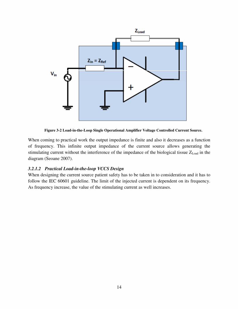
Figure 3-2 Load-in-the-Loop Single Operational Amplifier Voltage Controlled Current Source.

When coming to practical work the output impedance is finite and also it decreases as a function

of frequency. This infinite output impedance of the current source allows generating the

stimulating current without the interference of the impedance of the biological tissue ZLoad in the

diagram (Seoane 2007).

3.2.1.2 Practical Load-in-the-loop VCCS Design

When designing the current source patient safety has to be taken in to consideration and it has to

follow the IEC 60601 guideline. The limit of the injected current is dependent on its frequency.

As frequency increase, the value of the stimulating current as well increases.

15

Figure 3-3 Practical Single Operational Amplifier Voltage Controlled Current Source Design.

Adjusting Zin to the required value can give a freedom to control the injection current, hence the

name voltage controlled current source.

3.3 Data Acquisition and Analysis Hardware

3.3.1 National Instruments NI USB-6218

The NI USB-6218 is a plug-and-play USB connected data acquisition device. It is powered from

its USB bus. In this work the National Instruments NI USB-6218 is used as a multipurpose

hardware for:-. AC signal generation at the required frequency and amplitude to the current

source, measuring the response voltage from the test circuit are done using it.

The NI USB-6218 has 32 analog inputs when it is used in a single ended mode. This number is

reduced by half when it is applied in a differential mode. The sampling rate is dependent on the

number of analog inputs that are used. It is 250kS per second for a one analog input channel and

it is divided by the number of analog inputs when there are two or more analog channels are at

use. The input voltage range is ± 10 volts

Unlike the analog inputs the sampling rate of the analog outputs is not depend on the number of

channels used. It has two analog outputs with each channel update rate of 250kS per second.

Output voltage range is ± 10 volts. It has also eight digital inputs and outputs (National

Instruments 2011).

16

Figure 3-4 NI USB-6218.

3.3.2 Merits and Limitations of NI USB-6218

The first advantage of the NI USB-6218 is its bus-powered USB connection. This makes it easily

powered by a battery driven computer and in turn make the device safe for application on living

tissues. Its handy and compact design is an additional merit that is needed to construct a portable

medical device.

Low speed of sampling rate is one of its drawbacks. When coming to analog input sampling, the

division of the sampling rate to the corresponding number of analog inputs is another flaw. This

drawback makes a restriction in generating high frequency AC signals. The limited number of

analog output channel i.e. two, is also additional demerit of the NI USB-6218. This condition

limits the number of AC signals used in a multi-frequency application.

3.4 Measurement Systems

Before taking measurement using DAQ devices like the NI USB-6218 types of signal sources

and its measurement modes has to be noted. Below are the two types of signal sources and three

types of measurement modes are discussed.

3.4.1 Signal Sources

3.4.1.1 Grounded Signal Sources

This signal sources are connected to a systems ground. It also shares a common ground point

with the device in which the measurement has taken (National Instruments 2003a).

17

Figure 3-5 Grounded Signal Source.

3.4.1.2 Floating Signal Sources

In this type of signal sources, the voltage signal is not connected to any of common ground. The

measurement device’s ground point is not also connected to the signal source (National

Instruments 2003a).

Figure 3-6 Floating Signal Source.

3.4.2 Measurement Systems Modes

3.4.2.1 Differential Mode

Two channels of the measurement system are used for each signal and neither of these is

connected to a reference point like earth of the building etc. From its connection layout, it is seen

that it rejects common mode voltage (i.e. occurs when the measurement is taken between the

input and the reference or earth point and the voltage at the reference or earth point is not zero)

and noise (National Instruments 2003a).

18

Figure 3-7 Differential Mode Measurement Setup.

3.4.2.2 Referenced Single-Ended Mode (RSE)

The measurement is taken in-between the input and the ground point of the system (AIGND). In

this mode one channel is used in measuring each signal. Unlike the differential mode, RSE does

not reject the common mode voltage (National Instruments 2003a).

Figure 3-8 Referenced Single-Ended Mode Measurement Setup.

3.4.2.3 Non-Referenced Single-Ended Mode (NRSE)

In this mode measurements are taken with respect to a single analog input which is named

AISENSE (National Instruments 2003a).

19

Figure 3-9 Non-Referenced Single-Ended Mode (NRSE) Measurement Setup.

3.5 Laboratory Virtual Instrument Engineering Workbench (LabVIEW™)

This work has been entirely implemented using the National Instruments Laboratory Virtual

Instrument Engineering Workbench (LabVIEW). LabVIEW is a graphical programming

language. It is implemented using blocks of functions instead of lines of codes that are used in

text based programming languages. LabVIEW execution of the program follows the flow of

data, hence it is dataflow programming.

The LabVIEW’s user interface is called the Front Panel. The functional blocks are put in a

separate panel called the Block Diagram. The functional blocks put in Block Diagram controls

the Front Panel components (National Instruments 2003b).

3.6 Impedance Estimation Methods

Nowadays impedance measurement systems can be divided in two distinct approaches of

measurement methods, depending on the frequency contents of the stimulating signal. Therefore

the approaches are basically two: when the stimulation contains several frequencies and when a

single frequency is used to perform the measurement.

In multifrequency or multitone measurement signals, the stimulating signal applied to the

biological tissue contains two or more signals at different frequencies. If the number of tones is

sufficiently large and its distribution is broad enough, to get the impedance spectrum, a single

stimulation is enough. When using a single tone measurement; the exciting signal has a single

frequency(Seoane et al. 2008).On this approach the impedance spectrum can be obtained by

sweeping a single frequency through the range of the measurement.

The measurements taken by the above mentioned approaches are estimated in different manners

from the measured values of voltage and AC current (Seoane 2007). Digital Sine Correlation

20

(DSC), Total Least Square (TLS) and Fast Fourier Transform (FFT) are some of the available

estimation methods.

3.6.1 Single Frequency measurement Estimator

3.6.1.1 Digital Sine Correlation (DSC)

In this work Digital Sine Correlation (DSC) is implemented in estimating the impedance at a

single frequency measurement system. As biological tissue with impedance value of Z is excited

by applying a sinusoidal currentsin'ω5t) with a known value of amplitude I .Then the response

voltage Vm in the biological tissue is provided by:

-6'7( = . sin'*67( × ||∡

-6'7( = .|| sin'*67 + ( -6'7( = -6 sin'*67 + ([v]

-6'7( = -%9 sin'*67( + -%9 cos'*6 7( Equation 3.1

Equation 3.1 shows the response voltage is a cumulative of the voltage in phase with the injected

current with the voltage drop Vip, it is the voltage across the resistive part of the tissue and the

voltage with a 90° phase shift, i.e. in-quadrature, with the injected current with a voltage drop Viq,

it is the voltage across the reactive part of the tissue (Seoane 2007).

Figure 3-10 Digital Sine Correlation Estimation Method Block Diagram.

From the signal generator of the excitation, two sinusoidal signals one in phase and the other in-

quadrature with the injected current and having a unit value of amplitude A is generated as a

reference signal. These two signals modulate the two components of Equation 3.1 i.e. the in

phase component Vip is modulated by in phase reference signal and the in-quadrature component

Viq is modulated by the in-quadrature reference signal. These results ip(t) and iq(t) respectively

which is shown in the following equations (Seoane 2007).

21

:9'7( = ; sin'*67( -6 = ; sin'*67( [-%9 sin'*67( + -%< cos'*67(] :9'7( = ;-%9 sin'*67( + ;-%< sin'*67( cos'*67(] [A2

Ω]

Equation 3.2

Here applying double angle trigonometric relationship given below:

cos'2*67( = 1 − 2 sin'*67( = 2 cos cos'*67('*67( − 1

Equation 3.3

sin 2'*67( = 2 sin'*67( cos'*67( Equation 3.4

Inserting Equation 3.3 and Equation 3.4 to Equation 3.2 gives and ip(t) is solved as follows

:9'7( = ;-%9 =1 − cos'2*67(2 > + ;-%< =sin 2'*67(2 >

:9'7( = ;-%92 − ;-%9cos'2*67(2 + ;-%< sin 2'*67(2

:9'7( = ;-%92 + ;-%<2 [sin 2'7( − cos'2*67(]

Equation 3.5

and iq(t) is solved from

:<'7( = ; cos'*67( -6 = ; cos'*67( [-%9 sin'*67( + -%< cos'*67(] :<'7( = ;-%9 cos'*67( sin'*67( + ;-%< cos'*67(] [A2

Ω]

Equation 3.6

Inserting Equation 3.2 and Equation 3.3 in Equation 3.6 gives

:<'7( = ;-%9 =sin 2'*67(2 > + ;-%< =1 + cos'2*67(2 >

:<'7( = ;-%<2 + ;-%<cos'2*67(2 + ;-%9 sin 2'*67(2

:<'7( = ;-%<2 + ;-%92 [cos'2*67( + sin 2'*67(] Equation 3.7

From Equations 3.5 and 3.7 ip(t) and iq(t) are periodic with i?+ = @ABC and iD+ = @ABE

respectively. It can be deducted that

22

:9+ = ∫G:9'7(H7 = IJKL [A2

Ω]

Equation 3.8

:<+ = ∫G:<'7(H7 = IJKM [A2

Ω]

Equation 3.9

Since Vip and Viq are voltage drops across the resistive and reactive part of the tissue and I is the

amplitude of the injected voltage. Then the respective resistive part R and reactive part X can be

expressed as

= JKLN = %LO IPN = N ∫G:9'7(H7 [Ω]

Equation 3.10

= JKMN = %MO IPN = N ∫G:<'7(H7 [Ω]

Equation 3.11

From Equation 3.10 and 3.11 Z = R + jX can be found (Seoane 2007).The following block

diagram depicts the implementation of this method in this work.

23

Figure 3-11 Digital Sine Correlation LabVIEW Implementation.

24

3.6.2 Multifrequency Bioimpedance Measurement Estimators

3.6.2.1 Total Least Square (TLS) Method

The Total Least Square (TLS) is one of bioimpedance measurement estimation methods. In this

work the Singular Value Decomposition (SVD) is its computational tool to solve for solutions,

i.e.to solve for the resistive and reactive parts of the impedance of the biological material. It is a

continual derivation of Least Square (LS) method. Golub and Van Loan introduced it as a way of

solving system of equations that are called overdetermined system of equations of the form

; ≈ R

Equation 3.12

Where ; ∈ ℝU× and R ∈ ℝU×V are the know quantities and ∈ ℝ×V is the quantity to be

determined (I.Markovskya 2007).

The LS approach assumes that only the right side of Equation 3.12 which is B suffers from errors,

in this case noise, while the A part at the left side of the equation is free from it. But in practice

the error or noise is not restricted only in the right side of the equation. The error showed up in

both sides of the equation and this can be analogues to the measurement procedures; there are

errors in both sides of the measurement system, in this case in the current injection side and the

observation side as well. Here is TLS is useful when the errors are assumed to be occurred in

both sides of the equation (S. Van Huffel 1991).

Whenever r > c, i.e. the number of measurements are more than that of the channels in the

measurement system, exact solution is not derived for X instead the approximate value of it is

looked for (I.Markovskya 2007). Hence, TLS is applied to solve for the estimated values of X

when the system under study have disturbances, noises, errors or in general perturbation in both

sides, i.e. in both A and B.

Estimation of EBI using the TLS approach requires the in-phase and in-quadrature versions of

the injected current to the biological material under study and the observation voltage across the

biological material. These quantities can be collected using the same measurement setup as that

of Digital Sine Correlation (DSC) method with some modifications which is discussed in section

3.6.1.1 of this work. The modified measurement setup is shown below that is used to get the

components of EBI estimation implementing TLS approach.

25

Figure 3-12 Measurement Setup for EBI Estimation Using TLS with In-Phase (Sin (ωt)), In-Quadrature

(Cos (ωt)) and Measurement Voltage Vm.

It is shown in the figure that all the required quantities for the EBI estimation using TLS are

derived and presented. The box labeled VCCS is discussed in detail in the later section of this

work for the multifrequency measurement system.

3.6.2.1.1 Single Frequency Approach

At first the single frequency approach of the estimation is presented and its generalized

multifrequency approach is put afterwards.

To start with the measurement voltage Vm given by

-6'W( = :'W( × 'W(

Equation 3.13

When frequency * = *6

-6'W( = . sin'*6W( '*6( Equation 3.14

26

Z is a complex quantity at frequency *6 , and is given by

'*6( = '*6( + '*6( Equation 3.15

Since Vm is an additive combination of the voltage drops across the resistive and reactive part of

the bioimpedance and it can be expressed as

-6'W( = . sin'*6W( × '*6( + . cos'*6W( × '*6( Equation 3.16

As it is mentioned above Vm has two components that have sine and cosine functions. The part

that has a sine function which is given as

. sin'*6W( × '*6( Equation 3.17

is in-phase with the stimulating or injected current and represents the voltage drop across the

resistive part of the biological material. The part that has a cosine component given by

. cos'*6W( × '*6( Equation 3.18

is in-quadrature with the injected current and it gives a voltage drop across the reactive part of

the biological material.

Using matrix form of representation, the Equation 3.16 can be put in the following way

[. sin'*6W( . cos'*6W(] × X'*6('*6(Y = [-6'W(] Equation 3.19

A simplified version of this equation is given by

[.]U× × []× = [-6]U×

Equation 3.20

The TLS is an approach to solve equations like given in Equation 3.20 as it is discussed when

there is a perturbation on both sides of the equation. The perturbations in this case are the noises

in the reference current I in the left side and the observation voltage Vm across the biological

material in the right side and these noises are given ∆I and ∆Vm respectively.

The estimation of Z depends on the noise levels ∆I and ∆Vm that I and Vm respectively suffer. As

these noises become smaller the estimation become close to the true value. Applying the

perturbations ∆I and ∆Vm to Equation 3.20 equation

'. + ∆.(U× ×[× = '-6 + \-6(U×

Equation 3.21

27

Where [ is represents the estimated bioimpedance value.

Gloub and Van Loan stated in (G.H. Golub 1980) Equation 3.21 can be computed applying the

Singular Value Decomposition (SVD) for estimating the value of the [that represent estimated

bioimpedance value.

.[U× × [× =-]U×

Equation 3.22

Where .[ = '. +∆.(U× and

- = '-6 + \-6(U×

and its TLS solution can computed

[.|-6U×_ × X [−1Y_× ≈ 0

Equation 3.23

Application of the SVD to .|-6U×_ that is shown below when r > c, c = 3 in this particular case

a-b(.|-6U×_) = c × H:de(f, f, f_) ×-G Equation 3.24

Since the closest approximation h.[|-]6i of .|-6 that minimizes the perturbation is given by

h.[|-]6i = .|-6 − h∆.j|∆-j6i Equation 3.25

and its SVD is shown as follows

a-b(h.[|-]6i) = c × H:de(f, f, 0) ×-G

Equation 3.26

Then the perturbations h∆.j|∆-j6i obtained as

h∆.j|∆-j6i = h. − .[|-6 − -]6i = k_ × f_ × l_G

Equation 3.27

Then the approximation set is given as

h.[|-]6il_ = 0

Equation 3.28

its TLS solution is h.[|-]6iU×_ ×X [−1Y_× ≈ 0

Equation 3.29

28

and the estimated solution is given by

X [−1Y = − l_l_,_ − 1l_,_ hl,_, l,_iG

Equation 3.30

Since the estimated impedance [ is composed of the estimated resistive part ] and the

estimated reactive part ]and their estimated values are given from Equation 3.30 below

R = − mn,omo,oand ] = −l,_l_,_

Equation 3.31

This result show that the estimated values of the impedance at single frequency and in the

succeeding section its derivation for the multifrequency application of bioimpedance

measurement is given.

3.6.2.1.2 Multifrequency Total Least Square Approach

The measurement setup that is given in Figure 3-12 is also used in this multifrequency TLS

approach. As stated in the single frequency case the overdetermined system of equations ; ≈ R

where ; ∈ ℝU× and R ∈ ℝU×V are given or known values and ∈ ℝ×V is the estimation to be

determined.

From the given measurement setup the observation voltage Vm can be given as

-6(W) = :(W) × (W) Equation 3.32

Which can be written as the following at some frequency ω = ωm and with the stimulating or

injected sinusoidal current I,

-6(W) = . sin(*6W) × (*6) Equation 3.33

and the impedance Z is a complex quantity that can be given as at the same frequency ω = ωm

(*6) = (*6) + (*6)

Equation 3.34

Since here it is assumed that the injected current is given at several different frequencies, the

respective measurement voltages Vm at each time the measurement is taken are given as in the

following manner

29

-6,+(7+) = .+ sin(*+7+) × +(*+) + .+ cos(*+7+) ×+ + . sin(*7+) × (*) + . cos(*7+) ×(*) +…+ . sin(*7+) × (*) + . cos(*7+) ×(*) -6,(7) = .+ sin(*+7) × (*+) + .+ cos(*+7) ×+ + . sin(*7) × (*) + . cos(*7) ×(*) +…+ . sin(*7) × (*) + . cos(*7) ×(*)

…

… -6,U(7U) = .+ sin(*+7U) × (*+) + .+ cos(*+7U) ×+ + . sin(*7U) × (*) + . cos(*7U) ×(*) +…+ . sin(*7U) × (*) + . cos(*7U) ×(*)

Equation 3.35

Where Vm,0 ,Vm,1,…, Vm,r-1 are the measurement voltages taken at different times t0,t1,…,tr-1 with

the injected current at frequencies ω0, ω1,…, ωc-1 and r and c represents the number of times that

the measurement taken and the number of frequencies used in the measurement system

respectively.

The components with the sine function in Equation 3.35 at time t0 that are given as

.+ sin(*+7+) × +(*+) + . sin(*7+) × (*) +…+ . sin(*7+) × (*)

Equation 3.36

represents the respective resistive voltage drop across the impedance Z at that particular time and

it is in-phase with the injected currents of different frequencies to the biological material.

The remaining part that have cosine functions in Equation 3.35 given as

.+ cos(*+7+) ×+ +. cos(*7+) ×(*) + ⋯+. cos(*7+) ×(*)

Equation 3.37

represents the respective reactive voltage drop across the impedance Z at that particular time and

it is in-quadrature with the injected currents of different frequencies to the biological material.

The next step is putting the expression in Equation 3.35 in a matrix form, since it represents

measurements taken r times at c different measurement frequencies and r > c. The matrix format

of Equation 3.35 is given as

30

r .+ sin(*+7+). sin(*7+)⋯ . sin(*7+) .+ cos(*+7+). cos(*7+)⋯. cos(*7+).+ sin(*+7). sin(*7)⋯. sin(*7).+ cos(*+7). cos(*7)⋯. cos(*7)⋮.+ sin(*+7U) . sin(*7U)⋯. sin(*7U) .+ cos(*+7U). cos(*7U)⋯ . cos(*7U)t ×uvvvvw

+⋮+⋮xyyyyz = r -6,+-6,⋮-6,U

t

Equation 3.38

This matrix form representation can be put in a simpler form as

.U× ×× =-6,U×

Equation 3.39

When there is a small amount of noise in the injected current I and observation Vm, the

estimation of Z is closest to the true value. Assuming the perturbations ∆I and ∆Vm found in the

injected current I and observation voltage Vm respectively. The expression in Equation 3.39 can

be modified to include the noises on either side of it and the estimated impedance Z] is also given

as follows

'. + ∆.(U× × [× = '-6 + ∆-6(U×

Equation 3.40

And the respected estimated values given as

.[U× ×[× =-]6,U×

Equation 3.41

Where .[ = '. + ∆.(U× and

-]6 = '-6 + ∆-6(U×

Applying Gloub and Van Loan algorithm(G.H. Golub 1980) the TLS solution for Equation 3.41

is computed in the following expression

[.|-6U×() × X [−1Y = 0

Equation 3.42

Computing the Singular Value Decomposition (SVD) Equation 3.42 results

a-b|(.|-6) = c × diag(σ, σ, … , σ, σ) × V

Equation 3.43

Where σ1≥ σ2≥…≥ σc+1.

Since the closest approximation can be obtained in a condition that the deviation is minimized

and leads to the expression

h.[|-]6i = .|-6 − h∆.j|∆-j6i = c × diag(σ, σ, … , σ, 0) × V

Equation 3.44

31

Then h∆.j|∆-j6i = .|-6 − h.[|-]6i = c × σ ×V

Equation 3.45

After getting Equation 3.45, the TLS solution can be shown as

h.[|-]6iU×() × X [−1Y()× = 0

Equation 3.46

and X [−1Y()× =− 1l, l = − 1l, hl,, l,, … , l,i Equation 3.47

Since

[ = uvvvvw

+⋮+⋮xyyyyz

Equation 3.48

From Equation 3.47 and Equation 3.48 the estimation of the resistive and the reactive parts of the

biological material can be obtained at each particular measurement frequencies. These is shown

in the expressions below first the resistive part

]+ =− n,nn,n , ] =− ,nn,n , … , ] =− ,nn,n

Equation 3.49

Where R0, R1 ,…, Rc-1 are the estimated resistive values at the first, second ,…, and the cth

measurement frequencies where c is the number of measurement frequencies used.

and the reactive part is given as

]+ =− n,nn,n , ] =− ,nn,n , … , ] =− ,nn,n Equation 3.50

32

Where X0, X1 ,…, Xc-1 are the estimated reactance values at the first, second ,…, and the cth

measurement frequencies where c is the number of measurement frequencies used.

From equations Equation 3.49 and Equation 3.50 the estimated values of the impedance, the

resistive part and the reactive part can be obtained using the TLS by implementing the SVD as a

computational tool.

Below is the flow chart that is showing the implementation of the TLS in this work to measure

the resistive and reactive part of the bioimpedance that is represented by a 2R1C equivalent

circuit.

33

Figure 3-13 Multifrequency EBI Measurement System Implementation –Total Least Square Method.

34

The implementation is consists of the two NI USB-6218 DAQs, Voltage Controlled Current

Source (VCCS) and 2R1C parallel circuit.

3.6.2.1.2.1 NI USB-6218 DAQ

This device is used to generate the voltage to the VCCS and measure all the reference and the

response measurement voltage across the 2R1C parallel equivalent circuit. Its detail is discussed

in section 3.3 of this work. The basic reason to use two DAQs is the constraints on number of its

output channels. Each DAQ has two output channels but in this work four of them is needed and

the use of two DAQs comes to fulfill the required number of output channels. From these four

channels, four voltages at different frequencies are generated to make them as input for the

VCCS to inject a multifrequency excitation current to the 2R1C parallel equivalent circuit.

3.6.2.1.2.2 Multifrequency Voltage Controlled Current Source (VCCS)

The VCCS used for the multifrequency approach is basically the same as that of the single

frequency; it is a Load-in-the-Loop configuration that is discussed in detail in section 3.2.1 of

this work. The only different thing used here is the use of multiple inputs for the implementation

of multiple input voltages that are used to create multiple frequency current injection to the

2R1C parallel equivalent circuit.

The VCCS implemented is a simple inverting Summing amplifier. The numbers of the multiple

inputs are decided based on the number of the measurement frequencies that the system intend to

have, in this case four then four input branches are used. The following figure shows a simple

implementation of an inverting summing amplifier as VCCS that is used in this work.

Figure 3-14 Multifrequency EBI Measurement System VCCS.

35

3.6.2.2 Synchronization of the DAQs

The need for generation of multifrequency current injection leads to the use of two NI USB-6218

DAQs. The main reason for the application of the two DAQs is due to their limited number of

analog output channels, i.e. each DAQ has two analog output channels. In this work four

different measurement frequencies are used, hence two DAQs are used. The individual timers

that each DAQ have result in asynchronous reference voltages and measurement voltage that

give rise to erratic estimations on the reactive part of the impedance. These errors can easily be

shown in the phases of each of the reference voltages and measurement voltage. The phases of

the voltages show a significantly large variation instead of reasonably insignificant low

variations that can be resulted from the inaccuracies that occur in the measurement setup. These

discrepancies of phase that occur due to the asynchronous timers of the individual DAQs shown

in the following screen shoot of the system.

Figure 3-15 Plot showing the four reference voltages at frequencies 300, 1400, 2500 and 3600 Hz and the

measurement voltage before synchronization with their corresponding phase shifts at the right side of the

plot.

At the origin of the plot the waveforms start at different points which is the result of their phase

differences that is shown in the right side of the plot in degrees. From here it is obvious that

synchronization of the two DAQs is a first thing to do before acqusation of the referance voltages

and measurement voltage.

The synchronization of the devices is achieved by routing out the timing signals, i.e. analog

output sample clock and start trigger, of one of the devices to the other using the Programmable

Function Interface (PFI) channels that are connected with an external cable inbetween the

devices. The PFI signals can individually be configured as a timing input/output signal for

analog input and analog output respectivelly (National Instruments 2007).The result of this

synchronization is displyed in the plot below.

36


measurement voltage after synchronization with their corresponding phase shift at the right side of the plot.

It shows a remarkable improvement on the phase differences of the reference voltages and

measurement voltage and their phase is not varying erratically as the program executed

everytime. This is helpful in synthesizing and analyzing the signals after the measurement

takesplace.

At this level of synchronization also ,some of the reference voltages show a larger phase shift

compared to the others and it gives an estimation errors on the reactive component of the

impedance again, i.e.it gives positive reactive value, at those particular measurement frequencies.

As it is discussed above these phase shifts gives an error in the reactive part. Another approach

is also implemented to remove the time delay that is occurred due to these phase shifts. The time

delay that is occurred due to the phase shifts is given by the following expression

:aℎ:#7 = °360 × #

Equation 3.51

Where ϕ° is the phase shift in degrees and f is the measurement frequency (Sengpiel).

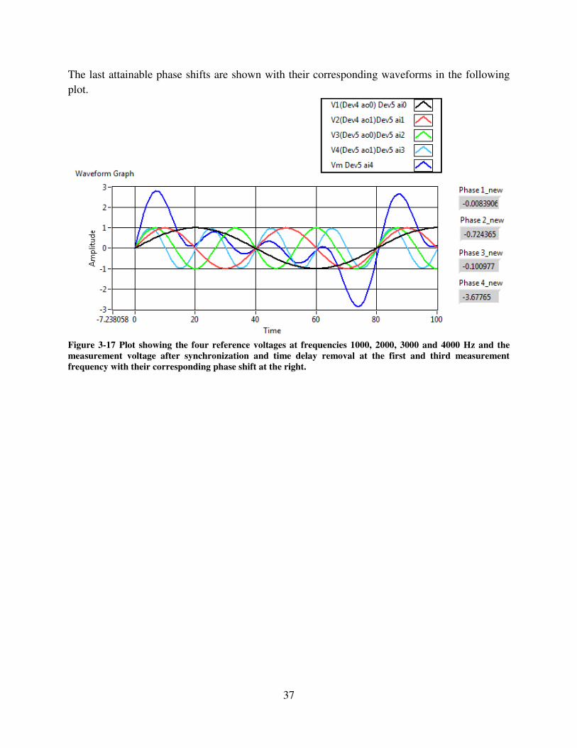
Finding and removing the time shift also has a limitation whenever the time delay is small

compared to the time between each samples i.e. sampling time. At the first and third

measurement frequencies this approach is successful since the time shift is almost equal to the

time difference between two samples or sampling time. But for the remaining measurement

frequencies it is not working due to their small time shift that result estimation errors i.e. the time

delay is smaller than the sampling time. The other problem this approach cannot overcome is the

phase shift at the measurement voltage. Since the measurement voltage is constructed with the

original waveforms not the time shifted signals, this gives an error in the estimation process.

37

The last attainable phase shifts are shown with their corresponding waveforms in the following

plot.


measurement voltage after synchronization and time delay removal at the first and third measurement

frequency with their corresponding phase shift at the right.

38

Chapter 4. Results

4.1 Measurement Results

The measurement results that are carried out during this work are presented in this chapter. The

first section contains the results from the single frequency impedance measurement set up and

later to that the results from the multifrequency impedance measurement system setup are

presented. As explained before, the single frequency impedance measurement setup is

implemented using DSC and the multifrequency impedance measurement setup uses Total Least

Squares.

4.2 Single Frequency Measurement

4.2.1 Single Frequency Measurement System GUI

To perform the spectroscopy measurement sweeping using a single frequency a GUI, with

controls and displays is build using LabVIEW. The controls are used to vary different parameters

of the measurement system like measurement frequency and amplitude sampling frequency,

number of periods etc. The waveform of voltages that are measured displayed using waveform

charts. The screenshot of the GUI is shown in the following figure below.

39

Figure 4-1 GUI of the Single Frequency Measurement system.

4.2.2 Single Frequency Measurement Results

The result presented at this section are impedance values from the measurements that are taken

across the 2R1C equivalent electrical circuit as a load in the set up which is shown in the Figure

3.3. The impedance estimation method used is the single sine correlation method for the single

frequency measurement implementation. The schematic connection is shown below.

Figure 4-2 Schematic Showing the measurement Setup with the (inset) 2R1C Equivalent Electrical

Circuit with Components.

The theoretical values are derived from those particular component values of the 2R1C shown in

the Figure 4-2 by calculating the equivalent impedance of it which is given by the following

formula which is derived in section 2.3 of this work.

= &'1 + %$*(1 + $*'% + &( Equation 4.1

The respective R and X values are computed at each measurement frequency from Equation 4.1

by taking the real and imaginary part of the complex Z value.

The calibration of the system performed using one 2R1C parallel circuit with 30nF capacitor in

series with 745.4 Ω resistor and in parallel with a 313.7 Ω resistor. Calibration of the estimated

measurements done against the theoretical values and a factor developed to improve the

estimation. The factor is given as a function of frequency in the following equation:

40

$d:Wd7:d7W'#( = ℎW7:d-dk'#(dkWH-dk'#(

Equation 4.2

Then to get the calibrated value for the measurements

$d:Wd7H-dk'#( = $d:Wd7:d7W'#( × dkW7-dk'#( Equation 4.3

The measurements are taken using two different sets of 2R1C circuits. The first set is a 20nF

capacitor in series with 996 Ω resistor and in parallel with a 596 Ω resistor and the second 2R1C

set is 40nF capacitor in series with 498.5 Ω resistor and in parallel with a 298 Ω resistor.

The measurements, calibrated and theoretical values from Equation 4.1, the two set of

measurements of 2R1C circuits are given in the following tables below. Table 4-1 gives the

resistive part of the measurement for the 2R1C circuit with 20nF.

Table 4-1 Single Frequency-Resistive Part Estimated, Theoretical and Calibrated values of 20nF 2R1C

Circuit.

Measurement Frequency

(Hz)

R (Ω) Estimated R (Ω) Theoretical R (Ω) Calibrated

100 597.337 595.9107349 596.988

200 596.889 595.6433678 596.54

400 596.423 594.5802787 596.074

600 593.598 592.8308333 594.089

800 590.331 590.4274864 590.82

1000 587.508 587.4135724 587.995

2000 561.484 565.2090284 565.023

3000 526.43 536.9127447 535.752

4000 492.508 508.8965249 507.611

5000 464.378 484.4056069 478.618

6000 438.867 464.2887508 460.067

7000 418.725 448.2263969 445.975

8000 401.916 435.5245981 428.072

9000 385.938 425.4755789 420.647

10000 373.857 417.4792903 407.479

20000 288.734 385.9924173 377.648

30000 212.365 378.9014734 369.103

40000 133.059 376.3051609 363.89

50000 50.6752 375.0822986 355.105

The reactive part of the measurements, calibrated and theoretical values, for the 2R1C parallel

circuit with 20nF are given in the following table.

41

Table 4-2 Single Frequency-Reactive Part Estimated, Theoretical and Calibrated values of 20nF 2R1C

Circuit.


(Hz)

X (Ω) Estimated X (Ω) Theoretical X (Ω) Calibrated

100 -6.02773 -4.461990097 -4.14061

200 -12.0697 -8.91328248 -8.291

400 -24.3575 -17.74149376 -16.7318

600 -36.0335 -26.40224776 -24.6797

800 -47.6947 -34.81835265 -32.6665

1000 -57.7785 -42.91998735 -39.5731

2000 -106.807 -76.95564268 -71.5871

3000 -140.354 -98.45088734 -90.6521

4000 -160.659 -108.8485288 -95.3402

5000 -174.528 -111.5628096 -103.571

6000 -180.564 -109.7283101 -96.5712

7000 -185.274 -105.5227001 -87.9756

8000 -187.992 -100.26874 -89.266

9000 -189.628 -94.7089773 -76.0091

10000 -192.241 -89.23509231 -77.0563

20000 -223.899 -39.3407 -52.48703656

30000 -258.362 -26.1699 -36.17284719

40000 -286.317 -19.5106 -27.45408261

50000 -268.367 -15.5869 -22.08551771

The pictorial representation of the results given in the Tables 4-1 and 4-2 are given in the

following two spectral and impedance plot.

42

Figure 4-3 Single Frequency-Plot of Frequency versus Resistance Measurement, Theoretical and

Calibrated values of 20nF 2R1C parallel model.

Figure 4-4 Single Frequency-Plot of Frequency versus Reactance Measurement, Theoretical and


0 1 2 3 4 5 6

x 104

0

100

200

300

400

500

600

Frequency(Hz)

Resis

tance(o

hm

)

Frequency versus Resistance

Theory 2R-1C Parallel

Theory 2R-1C Parallel Min

Theory 2R-1C Parallel Max

Measurement

Calibrated Meas

0 1 2 3 4 5 6

x 104

-300

-250

-200

-150

-100

-50

0

Frequency(Hz)

Reacta

nce(o

hm

)

Frequency versus Reactance




Measurement

Calibrated Meas

43

Figure 4-5 Single Frequency-Plot of Resistance versus Reactance Measurement, Theoretical and


The second measurement is taken using a 40nF for the capacitor in the 2R1C parallel circuit. The

following tables show the values obtained from the measurement, theoretical and calibrated

results for the resistive and reactive part of the impedance.

0 100 200 300 400 500 6000

50

100

150

200

250

300

Resistance(ohm)

-Reacta

nce(o

hm

)

Resistance versus Reactance


Measurement

Calibrated Meas

44

Table 4-3 Single Frequency-Resistive Part values, Theoretical and Calibrated, for 2R1C Circuit with 40nF.


(Hz)

R (Ω) Estimated R (Ω) Theoretical R (Ω) Calibrated

100 298.612 297.9553395 298.437

200 298.402 297.8215722 298.227

400 298.209 297.2896991 298.035

600 296.726 296.4144496 296.972

800 295.114 295.2120806 295.359

1000 293.758 293.7042972 294.001

2000 280.542 282.5975148 282.31

3000 263.241 268.4476495 267.903

4000 246.08 254.4422743 253.626

5000 232.975 242.2028244 240.119

6000 219.374 232.1518561 229.971

7000 209.211 224.1282693 222.827

8000 200.992 217.784399 214.072

9000 192.457 212.766093 209.765

10000 186.44 208.7732905 203.208

20000 144.325 193.0543804 188.769

30000 104.97 189.5152002 182.444

40000 65.0211 188.2194182 177.82

50000 23.5723 187.6091184 165.183

The table below gives the reactive values for the part of the measurement, both calibrated and

theoretical, from measurements on the 2R1C parallel circuit with 40nF.

45

Table 4-4 Single Frequency- Reactive Part values, Theoretical and Calibrated for 2R1C Circuit with 40nF.


(Hz)

X (Ω) Estimated X (Ω) Theoretical X (Ω) Calibrated

100 -3.05319 -2.230993927 -2.09731

200 -6.10805 -4.456632289 -4.19578

400 -12.2795 -8.870675948 -8.43508

600 -17.961 -13.20088826 -12.3017

800 -24.0683 -17.40862995 -16.4846

1000 -29.5488 -21.45895592 -20.2383

2000 -53.5885 -38.4711497 -35.9174

3000 -70.2842 -49.20906748 -45.3953

4000 -80.1762 -54.39757807 -47.5793

5000 -86.6348 -55.74636733 -51.412

6000 -90.2261 -54.82348608 -48.2556

7000 -92.5229 -52.71747423 -43.9336

8000 -93.7881 -50.08909845 -44.5343

9000 -94.8021 -47.30905217 -37.9997

10000 -95.6279 -44.5727303 -38.3307

20000 -112.577 -26.21251429 -19.7805

30000 -130.413 -18.06433578 -13.2097

40000 -144.566 -13.7100771 -9.85118

50000 -135.133 -11.02903608 -7.84863

The pictorial representation of the results given in the Tables 4-3 and 4-4 are given below. The

plots are presented in spectral plots and an impedance plot i.e. resistance against reactance.

46

Figure 4-6 Single Frequency-Plot of Frequency versus Resistance Measurement, Theoretical and


Figure 4-7 Single Frequency-Plot of Frequency versus Reactance Measurement, Theoretical and


0 1 2 3 4 5 6

x 104

0

50

100

150

200

250

300

Frequency(Hz)

Resis

tance(o

hm

)





Measurement

Calibrated Meas

0 1 2 3 4 5 6

x 104

-150

-100

-50

0

Frequency(Hz)

Reacta

nce(o

hm

)





Measurement

Calibrated Meas

47

Figure 4-8 Single Frequency-Plot of Resistance versus Reactance Measurement, Theoretical and


4.3 Multifrequency Measurement

4.3.1 Multifrequency Measurement System GUI

The GUI for the multifrequency measurement system is used to perform measurements of

impedance on a 2R1C parallel equivalent circuit. The GUI has different controls to give the

necessary inputs for the system to operate. These include the value for the measurement

frequencies, the sampling configuration i.e. the sampling frequency and number of samples per

channels. The other controls are amplitude and phase of the signal to be injected. In addition to

the controls, the GUI has different displays to show the intermediate voltage waveforms of the

measurement and the measured and calibrated result values. A screenshot is shown in figure 4-9.

0 50 100 150 200 250 3000

50

100

150

Resistance(ohm)

-Reacta

nce(o

hm

)



Measurement

Calibrated Meas

48

Figure 4-9 GUI of the Multifrequency Measurement system.

4.3.2 Multifrequency Measurement Results

The measurements using multifrequency setup are done using 4 different measurement

frequencies i.e. 300, 1400, 2500 and 3600 Hz. Before performing calibration, samples of

measurements were taken using the two possible measurement setups on 2R1C circuit. The first

approach, measure the reference voltages and the measurement voltage using only one DAQ

board. In the second approach, a measurement is taken by both the two DAQ boards. The later

approach gives a higher sampling frequency since the measurement channels are shared between

the two DAQs. Mean Absolute Error (MAE) and Standard Deviation (STD) are calculated for

each of the approaches at different number of samples. The purpose of taking sample

measurements at different number of samples is to get the least error resulting scenario. The

measurement is performed using 2R1C circuit with 20µF capacitor in series with 2981 Ω resistor

and in parallel with a 998 Ω resistor.

The comparison of MAE and STD of the two approaches from the Tables 5-3 and 5-4, which are

given below shows that the measurements using two DAQ boards produces smaller MAE and

STD compared with using only one DAQ board.

Accordingly these results and the fact that a higher sampling frequency is obtained makes the

two DAQs measurement approach a measurement setup of choice for this work. Regarding the

49

number of samples to be used for the measurement there is no a remarkable difference on the

results when using a small or larger number of samples. Hence, for the purpose of this work

1000 samples are used during the measurements.

Figure 4-10 shows the circuit implementation of the VCCS load-in-the-loop for a multifrequency

measurement. Here 2R1C circuit with 20nF shown for illustration purpose.

Figure 4-10 Voltage Controlled Current Source with the 2R1C Parallel Model in Multifrequency

Impedance Measurment.

50

Table 4-5 Measurement Mean Absolute Errors (MAE) and Standard Deviation (STD) of Two DAQs measurement setup at Sampling Frequency of

80kHz.

Samp(Time) 200samp(2.5ms) Samp(Time) 1000samp(12.5 ms)

f (Hz) MAE R (STD) MAE X (STD) f (Hz) MAE R (STD) MAE X (STD)

300 27.36660024(0.163375) 1.438235(0.090046) 300 6.473300235(0.073976) 0.239995026(0.018384)

1400 5.350317312(0.149265) 7.740402(0.077286) 1400 0.660282688(0.076222) 4.432102487(0.030975)

2500 0.330976793(0.130178) 1.508098(0.334596) 2500 1.987523207(0.053697 7.286898239(0.037139)

3600 2.369428197(0.118857) 35.04358(0.137054) 3600 3.491128197(0.044717) 33.12081373(0.092982)

Samp(Time) 5000samp(62.5ms) Samp(Time) 25000samp(0.3125s)


300 2.279700235(0.090112) 1.274715(0.006831) 300 1.444700235(0.153931) 1.538895(0.016969)

1400 2.062882688(0.075884) 2.469802(0.012173) 1400 2.403982688(0.114907) 2.036502(0.020946)

2500 2.367123207(0.070281) 8.700198(0.014538) 2500 2.469523207(0.093216) 8.978598(0.026671)

3600 3.743228197(0.059305) 32.93136(0.019729) 3600 3.778128197(0.08509) 32.90547(0.024677)

Samp(Time) 40000samp(0.5s)

f (Hz) MAE R (STD) MAE X (STD)

300 1.1792(0.119685) 1.59296503(0.007631)

1400 2.442683(0.07431) 1.93310249(0.01957)

2500 2.469223(0.058942) 9.043398(0.023148)

3600 3.802028 (0.050899) 32.9017(0.021105)

51

Table 4-6 Measurement Mean Absolute Errors (MAE) and Standard Deviation (STD) for one DAQ measurement setup at Sampling Frequency

50 kHz

Samp(Time) 200samp(2.5ms) Samp(Time) 1000samp(12.5 ms)


300 0.325100094(0.318257) 7.530375(0.0362) 300 0.399400188(0.255799) 1.264204974(0.313005)

1400 14.14131731(0.167626) 42.76987(0.179391) 1400 5.410417312(0.222913) 35.55931249(0.172242)

2500 13.55897679(0.138129) 24.54227(0.063849) 2500 8.174476793(0.200273) 15.32300176(0.103968)

3600 11.8884282(0.134091) 8.636424(0.04929) 3600 4.419928197(0.185468) 7.617803729(0.049344)

Samp(Time) 5000samp(62.5ms) Samp(Time) 25000samp(0.3125s)


300 0.386500235(0.154044) 0.927455(0.014905) 300 0.333600235(0.131505) 0.844125(0.007142)

1400 5.503317312(0.12946) 35.40059(0.02538) 1400 5.559017312(0.102237) 35.3574(0.019267)

2500 8.267776793(0.114404) 15.1781(0.029904) 2500 8.318776793(0.083502) 15.1333(0.018438)

3600 4.505228197(0.101806) 7.472314(0.026529) 3600 4.550328197(0.07488) 7.435014(0.015004)

Samp(Time) 40000samp(0.5s)

f (Hz) MAE R (STD) MAE X (STD)

300 0.3588(0.187176) 0.839405(0.012531)

1400 5.552517(0.152347) 35.36015(0.028119)

2500 8.314277(0.133958) 15.1338(0.030441)

3600 4.549028(0.121909) 7.435144(0.022903)

52

The calibration work of the system has been performed using one 2R1C circuit with 30nF

capacitor in series with 2100.7 Ω resistor and in parallel with a 548.2 Ω resistor. In section 4.2.2

the method for finding the calibration factors has been introduced. The measurements are taken

using two different sets of 2R1C circuits. The first set is with a 20nF capacitor in series with

2981 Ω resistor and in parallel with a 998 Ω resistor and the second 2R1C set is with 40nF

capacitor in series with 1292.8 Ω resistor and in parallel with a 695.7 Ω resistor.

The measurements, calibrated and theoretical values, obtained from the two set of the mentioned

2R1C circuits are given in the following tables below. Table 4-5 gives the resistive part of the

measurement for 2R1C circuit with 20nF.

Table 4-7 Resistive Part Estimated, Theoretical and Calibrated values for 2R1C Circuit with 20nF.

Measurement Frequency (Hz) R (Ω) Estimated R (Ω) Theoretical R (Ω) Calibrated

300 986.732 992.4915 991.499

1400 915.882 915.6781 915.83

2500 844.33 845.365 844.11

3600 810.882 806.7186 810.882

The result obtained of the reactive component of the impedance from the same 2R1C circuit with

20nF is given in the next table, below. It shows the measurement estimation of the reactive part

of the impedance with the corresponding theoretical and calibrated values.

Table 4-8 Reactive Part Estimated, Theoretical and Calibrated values for 2R1C Circuit with 20nF.

Measurement Frequency (Hz) X(Ω) Estimated X(Ω) Theoretical X(Ω) Calibrated

300 -36.9086 -36.7222 -36.7838

1400 -113.182 -117.599 -119.705

2500 -129.717 -122.104 -122.041

3600 -73.6061 -106.264 -125.295

The pictorial representation of the result is given in the following two spectral plots and

impedance plot i.e. resistance against reactance.

53

Figure 4-11 Plot of Frequency versus Resistance Measurement, Theoretical and Calibrated values of

2R1C circuit with 20nF.

Figure 4-12 Plot of Frequency versus Reactance Measurement, Theoretical and Calibrated values of


0 500 1000 1500 2000 2500 3000 3500 4000 4500 5000750

800

850

900

950

1000

Frequency(Hz)

Resis

tance(o

hm

)





Measurement

Calibrated Meas

0 500 1000 1500 2000 2500 3000 3500 4000 4500 5000-140

-120

-100

-80

-60

-40

-20

0

Frequency(Hz)

Reacta

nce(o

hm

)





Measurement

Calibrated Meas

54

Figure 4-13 Plot of Resistance versus Reactance Measurement, Theoretical and Calibrated values of


The second measurement is taken using a 40nF for the capacitor in the 2R1C parallel circuit. The

following tables show the values obtained from the measurement, theoretical and calibrated

results for the resistive and reactive part of the impedance.

Table 4-9 Resistive Part Estimated, Theoretical and Calibrated values for 2R1C Circuit with 40nF.

Measurement Frequency (Hz) R (Ω) Estimated R (Ω) Theoretical R (Ω) Calibrated

300 684.997 690.349 688.306

1400 614.365 615.7067 614.331

2500 544.568 547.3407 544.427

3600 512.69 509.7479 509.684

Table 4-10 shows the measurement, theoretical and calibrated reactive values of the 2R1C circuit

with 40nF.

Table 4-10 Reactive Part Estimated, Theoretical and Calibrated values for 2R1C Circuit with 40nF.

Measurement Frequency (Hz) X (Ω) Estimated X (Ω) Theoretical X (Ω) Calibrated

300 -36.192 -35.6903 -36.0697

1400 -110.724 -114.33 -117.106

2500 -121.621 -118.743 -114.424

3600 -80.377 -103.355 -136.821

750 800 850 900 950 10000

20

40

60

80

100

120

140

Resistance(ohm)

-Reacta

nce(o

hm

)



Measurement

Calibrated Meas

55

The pictorial representation of the results from the 2R1C circuit with 40nF is given in the

following plots as spectral plots and impedance plot.

Figure 4-14 Plot of Frequency versus Resistance Measurement, Theoretical and Calibrated values of


0 500 1000 1500 2000 2500 3000 3500 4000 4500 5000450

500

550

600

650

700

Frequency(Hz)

Resis

tance(o

hm

)





Measurement

Calibrated Meas

56

Figure 4-15 Plot of Frequency versus Reactance Measurement, Theoretical and Calibrated values of


Figure 4-16 Plot of Resistance versus Reactance Measurement, Theoretical and Calibrated values of


0 500 1000 1500 2000 2500 3000 3500 4000 4500 5000-140

-120

-100

-80

-60

-40

-20

0

Frequency(Hz)

Reacta

nce(o

hm

)





Measurement

Calibrated Meas

450 500 550 600 650 7000

20

40

60

80

100

120

140

Resistance(ohm)

-Reacta

nce(o

hm

)



Measurement

Calibrated Meas

57

Chapter 5. Discussion

The building of configurable bioimpedance spectroscope using NI USB-6218 and an additional

analog circuit is shown in this work. The measurements were performed at a single measurement

frequency and multiple measurement frequencies. Digital Sine Correlation (DSC) and Total

Least Square methods are used for the determination of single frequency and multifreqency

measurement bioimpedance respectively.

The first section of this work dealt with the estimation of impedance with the DSC method. It

shows that, the resistive and reactive components of the impedance at a single frequency can be

measured using the NI USB-6218 with an additional analog circuit that is used as a VCCS. The

implementation of the DSC is done using the LabVIEW development environment.

Measurements are taken after calibration has been done on a known set of 2R1C parallel model

of biological tissue. The measurements are taken at a frequency range of 100Hz to 50 kHz. The

results from the raw measurements before the calibration in part 4.2.2 shows that as the

measurement frequency increases the error increases as well, especially in the reactive part of the

impedance. This error is a result of high frequency effects in creating a stray capacitance in the

cables, connections and components in the circuit setup of the measurement system. After

calibration, applying the calibration factors on the performed raw measurements, the errors on

the resistive and reactive values are reasonably reduced.

Building the bioimpedance spectroscope for the multifrequency estimation of impedance

measurement was the second task of this work. Total Least Square method is the mathematical

tool implemented to recover the components of the impedance. It used LabVIEW development

environment as in the case of DSC. The multifrequency estimation of the impedance used two NI

USB-6218 DAQs for generation and measurement of the voltages that are used in analysis of the

impedances using the TLS method. When applying two devices for generation and measurement,

a problem of synchronizing the devices arose, since both acquisition cards operate on their own

independent timers. This asynchrony leads to the incorrect estimation of the components of the

impedance under study, especially on the higher frequencies and the reactive part of the

impedance. Overcoming this asynchrony on the DAQs was the first step in the building of the

bioimpedance meter of this particular work. Two alternatives were implemented to overcome

this problem of asynchrony of the DAQs. The first thing that is performed on the system is

routing out the timing signals of one of the DAQ to the other with the PFI channels. The PFI

channels that are intended to the routing on each of the DAQs then connected using an external

cable. As it has been shown in section 3.6.2.2 of this thesis report, this alternative produced a

remarkable improvement on the synchronization of the reference voltages and measurement

voltage. After such timing signals synchronization approach and since, the measurement signals

were not fully synchronized yet, hence a second approach was implemented on the individual

reference voltages that were still not synchronized. This approach mainly dealt with a phase shift

observed on the voltage signals. The synchronization was produced by removing the length of

the time shift that produced the asynchrony from the total length of the voltage measured signal.

58

Such time shift is dependent on the individual measurement frequencies and the sampling

frequency of the system. This second alternative synchronized the reference voltages that were

not able to reach a full synchronization in the first step. Either way , there were signals that

cannot be synchronized completely due to their smaller time shift compared to the sampling time,

i.e. since the length of the time shift is less than that of sampling time, it is not possible to

remove that length of the time shift.

The influence of the number of samples on the estimation of impedance when using the TLS

approach was also studied. Verifying this was done by taking measurements with different

number of samples and calculating their mean absolute error and standard deviation. It was learnt

that there is no such a difference among the used number of samples and one of the number of

samples i.e. 1000 was taken. Additionally, the measurement configurations i.e. using one of the

DAQs or both the DAQs for the measurement were also studied. The use of two DAQs give a

higher sampling frequency, this in turn gives a higher measurement frequency, and produces

lower mean absolute error and standard deviation compared to that of the one DAQ measurement

setup. Due to these reasons two DAQs measurement approach is chosen for the implementation

of the measurement system for multifrequency impedance estimation.

As it is discussed the measurements are taken after calibration has been done on the system with

a known 2R1C parallel circuit. The results shown in section 4.3.2 depict that the calibrated

values are close to the theoretical ones in measurement frequencies that are nearly synchronized.

In frequency points that are not fully synchronized the calibrated results are not near compared to

that of the synchronized ones. In general, with the asynchrony of the signals, the resulting

calibrated measurements are giving the intended results.

It is not feasible to compare the performance of the two methods, DSC and TLS, since the errors

that come with the use of two DAQs is not totally avoidable from the measurement system.

59

Chapter 6. Conclusion and Future Work

6.1 Conclusion

Building a custom made bioimpedance meter using the NI USB-6218 is the main goal of this

work and performance comparison of the two estimation methods of bioimpedance, i.e.

frequency sweeping with Digital Sine Correlation and Digital Deconvolution with Total Least

Square, is the other task. It is shown that building the custom made bioimpedance spectroscope

is attainable with the use of NI USB-6218 DAQ for single and multifrequency measurements. It

is learned that this custom made measurement setup can measure impedance with the above

mentioned estimation methods of bioimpedance even if it has problems that come with the

hardware specifications that the setup is built i.e. using two different DAQ boards.

It can be configured for a specific type of study at the internal building blocks level like the

estimation blocks and different controls including sampling frequency, number of samples, phase

and amplitude of the measurement signals. From these options that the system can offer, the

possibility to study the effects of the building blocks and the controls of the measurement

process on the bioimpedance estimations methods and on the estimation itself. The commercially

available devices that do not have an option to configure at the internal building blocks level can

be replaced by such a custom made configurable bioimpedance spectroscope.

6.2 Future work

The set up that is built in this work can be extended further by tackling the problems encountered

in this presented work. As a further work on this project

• Improving the measurement frequency range by using a high speed DAQs.

• Reducing the problem of asynchrony by implementing an analog circuitry that has a

capacity to generate a multifrequency voltage signals like Voltage Controlled Oscillators

(VCO).

• Solving Problem regarding the asynchrony of measurement signals by the use of one

DAQ with more output channels for the generation and measurement purpose.

• Optimizing the LabVIEW’s Virtual Instruments (VI) code by reducing redundant

sections of it using subVIs.

60

References

G.H. Golub, CFVL 1980, 'An Analysis of the Total Least Squares Problem', Society for

Industrial and Applied Mathematics Journal vol. 17, no. 6, p. 11. Gerard J. Tortora, BD 2007, Introduction to the Human Body : The Essentials of Anatomy and

Physiology, Seven edn, Wiley, cop, New York. I.Markovskya, SVH 2007, 'Overview of Total Least-Squares Methods', Signal Processing vol.

87, pp. 2283–2302. M.Tengvall, LE, V. Malmros, N. Bosaeus, L. Lissner, I. Bosaeus 2009, 'Body Composition in

the Elderly: Reference Values and Bioelectrical Impedance Spectroscopy to Predict Total Body Skeletal Muscle Mass', Clinical Nutrition, vol. 28, pp. 52-58. National Instruments, C 2003a, Labview Measurements Manual, NI Corporation, National

Instruments Corporation, Austin, pp. 24,25,28,31. National Instruments, C 2003b, Labview User Manual, NI Corporation, National Instruments

Corporation, Austin, p. 22. National Instruments, C 2007, Daq M Seriesn Ni Usb-621x User Manual Bus-Powered M Series

Usb Devices, C National Instruments, National Instruments, Corporation pp. 9-1. National Instruments, C, Ni Usb-6218, National Instruments Corporation. Available from:

<http://sine.ni.com/nips/cds/view/p/lang/en/nid/203484>. [20 January ]. P.Schwan, H 2001, Selected Papers by Herman P.Schwan, Oslo. Patterson, R (ed.) 2000, The Biomedical Engineering Handbook, Second edn, CRC Press LLC,

Boca Raton. R. Gordon, RL, M. Min, T. Parve, R. Salo 2005, 'A Virtual System for Simultaneous Multi-

Frequency Measurement of Electrical Bioimpedance', IJBEM, vol. 7, no. 1, pp. 243-246. S. Van Huffel, JV 1991, 'Introduction', in The Total Least Squares Problem

Computational Aspects and Analysis

Society for Industrial and Applied Mathematics, Philadelphia, p. 84. Sengpiel, E, Calculation of Phase Angle:Phase Differenece,Phase Shift from Time Delay,Time of

Arrival Differencr and Frequency. Available from: <http://www.sengpielaudio.com/calculator-timedelayphase.htm>. [Feburary 17].

Seoane, F 2007, Electrical Bioimpedance Cerebral Monitoring:Fundamental Steps Towards Clinical Application, PhD Thesis Chalmers university of Technology.

Seoane, F, Bragós, R, Lindecrantz, K, et al. 2008, Current Source Design for Electrical

Bioimpedance Spectroscopy in Encyclopedia of Healthcare Information Systems, vol. I A-D, EG Nilmini Wickramasinghe, IGI Global, Hershey PA, pp. 359-367.

Seoane, F, Macías, R, Bragós, R, et al. 2011, 'Simple Voltage-Controlled Current Source for Wideband Electrical Bioimpedance Spectroscopy: Circuit Dependences and Limitations ', Measurement Science and Technology, vol. 22, p. 12.

Storr, W, January 2012 Electronics Tutorial About Operational Amplifiers, Electronics-Tutorials.ws. Available from:

<http://www.electronics-tutorials.ws/opamp/opamp_1.html>. [20 January]. Sverre Grimnes, ØGM 2006, Bioimpedance in Wiley Encyclopedia of Biomedical Engineering,

ØGM Sverre Grimnes, John Wiley & Sons, Inc., Oslo, pp. 1-9. Sverre Grimnes, ØGM 2008, Bioimpedance and Bioelectricity Basics, Second edn, Elsevier Ltd.,

Oslo.

61

Tabuenca, Jg 2009, Multichannel Bioimpedance Measurement, Master of Science Thesis, Tampere University of Technology.

Ursula G. Kyle, IB, Antonio D. De Lorenzo,Paul Deurenberg, Marinos Elia, Josè Manuel Gòmez,Berit Lilienthal Heitmann, Luisa Kent-Smith, Jean-Claude Melchior,Matthias Pirlich, Hermann Scharfettek, Annemie M.W.J. Schols,Claude Pichard, Composition of the ESPEN Working Group 2004, 'Bioelectrical Impedance Analysis-Part I: Review of Principles and Methods', Clinical Nutrition, vol. 23, p. 1228.

Zilico, L, Electrical Impedance Spectroscopy Zilico Ltd Available from:

<http://www.zilico.co.uk/research_development/electrical_impedance_spectroscopy>. [10 May].

62

Appendix

Appendix A.1 NI USB-6218 Specification Summary *

General

Product Name USB-6218

Product Family Multifunction Data Acquisition

Form Factor USB

Part Number 779678-01

Operating System/Target Linux, Mac OS, Windows

DAQ Product Family M Series

Measurement Type Voltage

Isolation Type Bank Isolation

RoHS Compliant Yes

Analog Input

Channels 32, 16

Single-Ended Channels 32

Differential Channels 16

Resolution 16 bits

Sample Rate 250 kS/s

Max Voltage 10 V

Maximum Voltage Range -10 V, 10 V

Maximum Voltage Range Accuracy 2.69 mV

Maximum Voltage Range Sensitivity 91.6 µV

Minimum Voltage Range -200 mV, 200 mV

Minimum Voltage Range Accuracy 0.088 mV

Minimum Voltage Range Sensitivity 4.8 µV

Number of Ranges 4

Simultaneous Sampling No

On-Board Memory 4095 samples

Analog Output

Channels 2

Resolution 16 bits

Max Voltage 10 V

Maximum Voltage Range -10 V, 10 V

Maximum Voltage Range Accuracy 3.512 mV

Minimum Voltage Range -10 V, 10 V

Minimum Voltage Range Accuracy 3.512 mV

Update Rate 250 kS/s

Current Drive Single 2 mA

63

Current Drive All 4 mA

Digital I/O

Bidirectional Channels 0

Input-Only Channels 8

Output-Only Channels 8

Number of Channels 0, 8

Timing Software

Logic Levels TTL

Input Current Flow Sinking

Output Current Flow Sourcing

Programmable Input Filters No

Supports Programmable Power-Up States? Yes

Current Drive Single 16 mA

Current Drive All 50 mA

Watchdog Timer No

Supports Handshaking I/O? No

Supports Pattern I/O? No

Maximum Input Range 0 V, 5.25 V

Maximum Output Range 0 V, 3.8 V

Counter/Timers

Counters 2

Buffered Operations Yes

Debouncing/Glitch Removal Yes

GPS Synchronization No

Maximum Range 0 V, 5.25 V

Max Source Frequency 80 MHz

Pulse Generation Yes

Resolution 32 bits

Timebase Stability 50 ppm

Logic Levels TTL

Physical Specifications

Length 16.9 cm

Width 9.4 cm

Height 3.1 cm

I/O Connector Screw terminals

Timing/Triggering/Synchronization Triggering Digital

* The data is taken from http://sine.ni.com/nips/cds/view/p/lang/en/nid/203484.

64

Appendix A.2 NI USB-6218 Pinout *

* The figure is taken from National Instruments “DAQ M Series NI USB-621x User Manual”

page 164.

reconfigurable bioimpedance spectrometer for the...

Documents