reconfiguration strategies for mitigating the impacts of ... · the bap is an np-hard problem, and...
TRANSCRIPT

1
Reconfiguration Strategies for Mitigating the Impacts
of Port Disruptions
FINAL REPORT
METRANS Project 07-14
By
Petros Ioannou (Principal Investigator) Anastasios Chassiakos (co- Principal Investigator)
Afshin Abadi Hwan Chang Hossein Jula
Marios Lestas Lokesh Saggam David Thomas
Yun Wang
University of Southern California
Electrical Engineering - Systems, EEB 200B
Los Angeles, CA 90089-2562
and
California State University, Long Beach
College of Engineering
Long Beach, CA. 90840-5602
May, 2011
2
Disclaimer
The contents of this report reflect the views of the authors, who are responsible for the facts and
accuracy of the information presented herein. This document is disseminated under the
sponsorship of the Department of Transportation, University Transportation Centers Program,
and California Department of Transportation in the interest of information exchange. The U.S.
Government and California Department of Transportation assume no liability for the contents or
use thereof. The contents do not necessarily reflect the official views or policies of the State of
California or the Department of Transportation. This report does not constitute a standard,
specification, or regulation.

3
Abstract
Marine terminals and ports are designed to meet expected demands during normal operations in
order to facilitate the smooth and efficient movement of goods. Disruptive events may affect thes
e normal operations, and terminals, ports and regions must be prepared to mitigate such disruptio
ns in an effort to maintain the movement of goods.
In this project, we investigate methods of modeling and evaluating the port disruptions and
develop mitigation strategies for reducing the impacts of disruptions. The types of disruptions we
study in this work are assumed to occur at the local and regional levels. We show that disruptions
at the local level can be modeled as terminal allocation problems (TAP). The multi berth
allocation problem is viewed as a set partitioning problem, in which each partitioned problem
consists of a single berth allocation problem (BAP). Berth allocation is an essential logistics
operation, since, the deployment of other resources at a terminal have to be coordinated with the
berth allocation plan. The BAP is an NP-hard problem, and consequently heuristic methods
based on sub gradient and simulated annealing algorithms are developed to find a near-optimal
solution within a reasonable amount of time. Numerous experimental scenarios are developed to
evaluate the proposed BAP methodologies in the presence disruptions.
The problem at the regional level is to develop mitigation strategies so that the regional throughp
ut in moving goods is affected by the disruption at a minimal level. We look into the U.S. west co
ast region, consisting of multiple ports and the associated traffic network used for moving the go
ods within and out of the region. The regional service network is defined at a high level of aggre
gation, which includes the major ports and aggregated zones representing broad geographical des
tinations and intermediate zones. The network under disruption is modeled as the minimum cost
flow problem with binary constraints.
We demonstrated via examples that our methodology that relies on the use of optimization can m
inimize the effect of disruption at all levels.

4
Table of Contents List of Tables .......................................................................................................... 6
List of Figures ........................................................................................................ 7
Disclosure ............................................................................................................... 7
List of Acronyms and Abbreviations ................................................................... 8
1 Introduction ........................................................................................................... 9
2 Container Terminals and the BAP..................................................................... 12
2.1 Classifications of the BAP ........................................................................................ 13
2.2 Literature Review ...................................................................................................... 15
3 The Berth Allocation Problem (BAP) ................................................................ 16
3.1 The BAP Formulations ............................................................................................. 17
3.1.1 The Relative Positioning Formulation for the BAP ................................ 18
3.1.2 The Assignment Formulation for the BAP ............................................. 19
3.1.3 The Mixed Integer Linear Programming Formulation for the BAP ....... 20
3.1.4 Some Notes on Alternative Objective Functions .................................... 21
3.2 Solution Methods for the BAP .................................................................................. 23
3.2.1 The Lagrangian Relaxation Method for the BAP ................................... 23
3.2.2 The Simulated Annealing Method for the BAP ...................................... 28
3.2.2.1 Notation and Definitios ............................................................................... 29
3.2.2.2 Neighbor (candidate move) Search Procedure ............................................ 29
3.2.2.3 Acceptance Probability Funtion .................................................................. 30
3.2.2.4 Simulated Annealing Procedure.................................................................. 30
3.2.2.5 Initial Temperature and Cooling Rate ......................................................... 31
3.2.3 H1: Heuristic Method for an Initial Feasible Solution ............................ 32
3.2.3.1 Algorithm for an Initial Feasible Solution ................................................. 33
3.2.4 H2: Heuristic Method for an Improved Feasible Solution ...................... 34
3.2.4.1 Rectangle Movement Operators.................................................................. 34
3.2.4.2 Rectangle Movement Procedure ................................................................. 35
3.3 Computational Experiments for the BAP ................................................................. 37

5
3.3.1 CPLEX MIP: Computational Experiments ............................................. 38
3.3.2 Heuristic Methods: Computational Experiments .................................... 40
4 Terminal Allocation Problem (TAP) ................................................................. 42
4.1 Set Partitioning Problem ........................................................................................... 43
4.2 Solution Method for the TAP .................................................................................... 44
4.2.1 Notations and Definitions ....................................................................... 45
4.2.2 TAP Procedure ........................................................................................ 47
4.3 Port Disruptions Resulting in Partially Functional Berths ........................................ 48
4.4 Computational Experiments for the TAP .................................................................. 53
4.4.1 Case I: Vessels with Flexible Berthing Locations and Departure Times54
4.4.2 Case II: Vessels with Strict Berthing Locations and Departure Times .. 56
5 Disruption Mitigation at the Regional Level ..................................................... 58
5.1 Service Network Design ........................................................................................... 58
5.2 Service Network for the U.S. West Coast Region .................................................... 60
5.3 Mitigating Disruptions at Regional Level ................................................................. 63
5.4 Computational Experiments ...................................................................................... 67
5.4.1 Distributions of Freight from LA Port Node .......................................... 72
6 Overall Disruption Modeling and Mitigation ................................................... 74
6.1 TAP and Service Network Optimization (separately) ............................................ 786
6.2 Combination of TAP and Service Network Optimization ........................................ 80
7 Conclusions........................................................................................................... 83
References ............................................................................................................. 81

6
List of Tables Table 1: The rectangle movement operators ................................................................ 35 Table 2: Ranges of parameters α and b ....................................................................... 39 Table 3: Comparison between the BAP solutions using IP, SG, and SA ................... 39 Table 4: Performance comparison between SG and SA methods ............................... 41 Table 5: Experimental results scenarios 1 and 2 ........................................................ 54 Table 6: Experimental results scenarios 3 and 4 ......................................................... 55 Table 7: Experimental results scenarios 5 and 6 ......................................................... 57 Table 8: Experimental results scenarios 7 and 8........................................................... 57 Table 9: Import Freight Distribution (ton/day) via Major West Coast Ports................ 67 Table 10: Legends and numbers of nodes describing FAF zones ................................ 67 Table 11: Activation and transportation cost of sea links............................................. 69 Table 12: Estimating capacity (ton) of port links ......................................................... 70 Table 13: Estimating capacity of ground links ............................................................. 71 Table 14: Freight distribution from LA port by activating sea links ............................ 71 Table 15: Capacity of terminals.................................................................................... 74 Table 16: TAP optimization, container distribution ..................................................... 76 Table 17: Combined optimization, container distribution ............................................ 77

7
List of Figures
Figure 1: Space-time diagram for the berth allocation problem................................... 13 Figure 2: Changes in the original allocation due to changes in arrival time and service ........................................................................................................................... 14 Figure 3: Defining a vessel in the space-time diagram................................................. 17 Figure 4: Vessel-berth allocation in grid spaces ........................................................... 19 Figure 5: Possible optimal solutions under different cost functions............................. 23 Figure 6: Initial and final solutions by subgradient method ......................................... 28 Figure 7: Normalized objective values ......................................................................... 31 Figure 8: Average number of iterations and the number of minima............................. 32 Figure 9: Reduction by SWAPx resulting from Swap-Pair between ( )pS q and ( 1)pS q + followed by Push-Down 1( )pS q+ ′ .............................................................. 37 Figure 10: Reduction by RIGHT resulting from Push-Right of ( 1)pS q + followed by Push-Down 1( 1)pS q+ ′ + ................................................................................................... 37 Figure 11: Reduction by LEFT resulting from Push-Left of ( 1)pS q + followed by Push-Down 1( 1)pS q+ ′ + ................................................................................................... 37 Figure 12: Space-time diagram for the Terminal Allocation Problem ......................... 42 Figure 13: The TAP as a set partitioning problem........................................................ 44 Figure 14: Value of the block ....................................................................................... 45 Figure 15: Examples of partially functional berths....................................................... 49 Figure 16: Allocation on decomposed operational cells............................................... 51 Figure 17: Service network for the U.S. west cost region ............................................ 60 Figure 18: Reconfiguration of the regional service network ........................................ 62 Figure 19: Port (LA/LB) complex and adjacent road network ..................................... 73 Figure 20: Location of container terminals................................................................... 74 Figure 21: Baseline traffic flow .................................................................................... 75 Figure 22: Service network optimization, traffic flow.................................................. 77 Figure 23: Combined optimization, traffic flow........................................................... 78
Disclosure Project was funded in entirety under this contract to California Department of Transportation.

8
List of Acronyms and Abbreviations AGV: Automated Guided Vehicle
AP: Acceptance Probability
BAP: Berth Allocation Problem
B&B: Branch-Bound method
BOA: Berthed‐On‐Arrival
BTR: Berth‐Time‐Requested
CDF: Cumulative Distribution Function
ETA: Estimated‐Time‐Of‐Arrival
AF: Assignment Formulation for the Berth Allocation Problem
FCSN: Fixed Cost Service Network Formulation
MCFP: Minimum Cost Flow Problem Formulation
MCFPB: Minimum Cost Flow Problem Formulation with Binary constraints
MILPF: Mixed Integer Linear Programming Formulation for the BAP Problem
RPF: Relative Positioning Formulation for the Berth Allocation Problem
SSST: Separating the Set of Slack Transportation links in the MCFPB
H1: Heuristic 1
H2: Heuristic 2
IP: Integer Programming
mH1 : Modified Heuristic 1
MILP: Mixed Integer Linear Programming
PCU: Passenger Car Unit
LRπ : Relaxed Problem using Lagrangian Multiplier
D: Dual of Problem LRπ
SA: Simulated Annealing
SG: Subgradient
SPP: Set Partitioning Problem
TAP: Terminal Allocation Problem

9
1 Introduction
In today’s global economy, the oceans are becoming increasingly important for international
trade. Currently, more than 80% of the world’s trade travels by water. A very important
component of this global economic chain is container transport, since about half of the world’s
trade by value, and 90% of the general cargo, are transported in containers.
Shipping is the heart of the global economy, but it is vulnerable to attacks. Trade passes primarily
through a small number of hubs spread around the globe. Close to 75% of the world’s maritime
trade and half of its daily oil consumption pass through a handful of international straits and
canals. Hence, the international commerce is at great risk from attacks at one of the major trading
hubs or at one of a handful of strategic chokepoints [1],[2]. The adoption of a just-in-time
delivery approach to shipping by most industries, rather than stockpiling or maintaining
operating reserves, means that a disruption or slowing of the flow of almost any item can have
widespread implications for the overall market, as well as upon the national economy.
Disruptions to the maritime transportation system could be due to natural causes, (such as
hurricanes or earthquakes), or to man-caused activities (such as military surge or terrorism acts).
Moreover, the disruptions can be classified as predictable/anticipated (such as the longshoremen
strike), or unpredictable/unanticipated (such as a potential terrorist attack).
The location where the disruption occurs is a very critical parameter in determining the
disruption’s impact. For example, disruptions of operations in the ports on the west coast can
have a national impact, since the combined port of Long Beach/Los Angeles handles 33% of the
total container traffic in the US [3]. This huge volume moving through the local ports has very
serious effects not only at the local and regional levels, but on a national scale as well. As a
consequence the national economy has become heavily dependent on the smooth and reliable
operation of the west coast ports. This fact became quite evident during the 2002 longshoremen
strike at the Port of Los Angeles, which for 11 days crippled the nation at an estimated cost of
$1‐$2 billion per day [4].
In this study, we investigate methods of modeling and evaluating the effect of disruptions and
develop mitigation strategies for reducing their impact on port operations. The types of

10
disruptions we investigate are such that they can render a terminal partially or totally
non‐functional. These disruptions can be caused by equipment failure; physical damage to the
terminal berths due to natural or manmade disasters; delays caused by increased demands as in
the case of military surge, etc. Disruptions, caused by failure of one or more berths at terminals
within a single port, are related to the berth allocation problem (BAP), as it is referred to in the
literature. Berth allocation is an essential logistics operation for the management of container
terminals. According to the berth allocation plans, terminal operators are required to coordinate
the deployments of various resources within the ports so that containers are moved as smoothly
and as quickly as possible.
When a disruption takes place, the terminals might be unable to meet the expected demand, due
to partial or total loss of operational capabilities, or to a sharp rise in the demand (e.g. military
surge). Furthermore, such a disruption could affect several terminals within a particular port. It is
therefore critical to allocate berths to ships in such a way as to meet all demand, minimize the
vessel berthing time and maximize berth utilization. In order to mitigate the impacts of
disruptions, methods will be developed to re-route goods to different berths within the terminal,
or to different terminals within the ports so that the overall port throughput is affected as little as
possible. The question we will answer in this study is: how can we reassign ships to
berths/terminals within the same port, such that the overall port throughput is maintained.
In this study, we first address disruptions that can be handled on the local level i.e. by the termina
l itself via reallocation of resources or port level via reallocation of resources among terminals. D
isruptions that cannot be handled on the local level are studied on the regional level alone or in c
ombination with local level.
On the local level we consider the continuous BAP (as opposed to the discrete BAP), because it
is more diverse and more practical as a way of allocating resources on the berth level in order to
serve ships. Since the continuous BAP cannot be calculated in polynomially-bounded time [7],
we develop and implement some heuristic procedures based on sub gradient and simulated
annealing optimization methods, a set of systemic and efficient heuristics is implemented, in
order to find an initial feasible solution and to update a current solution by exploring a
sufficiently large solution space.

11
In addition to the BAP, we address the allocation of ships to multiple berths. This problem is
referred to as the terminal allocation problem (TAP). We will see that the TAP can be viewed as a
set partitioning problem, and hence it is an NP-hard problem. We develop a methodology based
on simulated annealing algorithm to solve the TAP.
The objective at the regional level is to develop mitigation strategies so that the effect of
disruption on the regional throughput is minimized. We consider the US west coast region,
consisting of multiple ports and the associated traffic network used for moving the goods within
and out of the region. The regional service network is defined at a high level of aggregation,
which includes the major ports and aggregated zones representing broad geographical
destinations and intermediary zones.
The flow of freight in the regional service network under normal operating conditions is modeled
as a minimum cost flow problem in which the disruption level is low enough to be handled by
ground transportation modes. When disruption occurs, the regional service network is
reconfigured to deal with the situation. For example, if the LA port zone is rendered non-
functional for a period of time, all services associated with the zone will either be discontinued
or operate at a lower capacity, which will affect its throughput capacity. The re-configuration of
the service network will involve opening sea transportation links between port zones. The
regional service network under disruption is modeled as a minimum cost flow problem with
binary (or, integer) constraints. It is solved by branch-and-bound method and a LP relaxation is
performed on every leaf of the branch-and-bound tree.
This report is organized as follows: In Section 2, the berth allocation problem (BAP) is described
and various formulations of the problem are presented. In Section 3, the BAP is modeled
analytically and two solution methods are developed. In Section 4, an extension to the BAP, the
terminal allocation problem (TAP), is studied. The TAP is modeled as asset partitioning problem,
and solution methods are proposed. The service network optimization is explained in Section 5.
In Section 6, the overall modeling and mitigation is demonstrated by an example. Finally,
Section 7 presents the conclusions.

12
2 Container Terminals and the BAP
A container terminal is a facility where containerized cargo is trans-shipped between ships and
land vehicles (trucks and trains). A terminal may have several wharfs (quays). Each quay consists
of several berths, which in turn are divided into sections. Each quay corresponds to a linear
stretch of space in the terminal. Container ships are moored at a berth of a terminal where they
are unloaded and loaded by gantry or quay cranes. Quay cranes traverse along the quay to
position containers at any point along the length of the ship. Quay cranes at berths load imported
containers on in-yard trucks, straddle carriers, or automated guided vehicles (AGVs). Quay
cranes also unload export containers from these vehicles into the ships. To maximize berth
utilization and minimize ship-turn-around time, ships should be optimally assigned and allocated
to berths. Hence, optimal allocation of berths to incoming ships will have a substantial impact on
logistics cost and level of service.
Usually, carriers inform the terminal operator of their estimated-time-of-arrival (ETA), latest
possible service completion (departure) time, and request a berthing time (called berth-time-
requested or BTR) several days in advance [5]. A vessel is said to be berthed-on-arrival (BOA)
if the mooring operation commences within 2 hours of arrival. The BOA statistics is often used
as an indicator to gauge the quality of service provided by the port operator [6].
Based on the information received, a terminal operator tries to satisfy the requested departure
times of every vessel by allocating one or more sections on a berth to calling vessels according to
their ETAs, estimated departure times, and BTRs. However, in cases when the arrival rate of
vessels is high, or unexpected arrivals occur, or any type of disruption happens at a terminal, it
may not be possible to serve all the vessels before their requested service completion time. Thus,
departures of some vessels may be delayed past the requested due time [5].

13
3000 1200600 900
121st
122nd
123rd
124th
00
00
0
Time [h]
Berth [m]
Figure 1: Space-time diagram for the berth allocation problem
Figure 1 illustrates the space-time diagram of a berth schedule. The horizontal axis represents the
berth length, while the time is represented by the vertical axis. Note that, in Figure 1, a vessel is
represented by a rectangle. The length of the vertical side of each rectangle represents the
duration of stay of a vessel at the berth, while the length of the horizontal side represents the
vessel length [5], [7]. Each calling vessel is characterized by its own space-time rectangle. These
rectangles cannot overlap either in the space or in the time dimension. The Berth Allocation
Problem (BAP) is to determine the optimal locations of those rectangles without overlaps [5]. In
other words, the BAP consists of optimally allocating and scheduling the berth space to calling
carriers such that the carriers are served within their time limits.
2.1 Classifications of the BAP
The BAP can be classified into the following two general categories:
1- Discrete vs. Continuous BAP:
In the continuous BAP, the berthing can be done in a continuum of locations along the berth
[8], [9]. In contrast, in the discrete BAP, the entire quay is divided into a countable number of
berths. In the discrete problem, it is assumed that, at each instant of time, at most one vessel
can be served at each berth.
It should be noted that a discrete BAP can be modeled as an unrelated parallel machine

14
scheduling problem, and the continuous BAP can be mapped into a two-dimensional cutting-
stock problem, which is an NP-Hard problem [7]. The focus of this study is on the continuous
BAP. The continuous BAP is more diverse and general. It can address the growing trends in
ship sizes, as there is a need for more flexible berth allocation planning. For instance, mega-
ships may sometimes moor across neighboring berths in order to enhance berth usage.
2. Static vs. Dynamic BAP
In Imai et al. [10], the static BAP refers to the problem in which all the ships are assumed to
have arrived at the port prior to the beginning of the berths’ scheduling. In contrast, the
dynamic BAP takes into account not only the ships that have already arrived at the time of
planning, but also those which will arrive later during the planning horizon. Furthermore, it is
assumed that the arrival times of all the ships are known a priori, hence re-planning is not an
issue.
In a general planning problem, however, the dynamic environment refers to the events whose
occurrences may change in time. For example, in the work by Moorthy and Teo [6], the
authors deliberately induce delays in the port stay time of vessels and increase the number of
vessels to evaluate their dynamic policy in a rolling horizon framework. That is to say that the
notion of dynamic BAP used in [10] is very limited and, therefore, we will use the second
notion in which the occurrence of events may change in time.
Berth
Time
Berth
Time
Berth
Time
(a) (c)(b)
Figure 2: Changes in the original allocation due to changes in arrival time and service time.
The original assignment of the ship, (b) delayed arrival time, and (c) delayed service time
Resulting from the terminal’s lack of resources (such as cranes and trucks)

15
Figure 2 demonstrates possible disruptions in an original berth allocation. These disruptions
may have occurred due to delays in vessel arrival time (Figure 2b), or vessel service time
(Figure 2c). If these unexpected delays make the original allocation plan unsatisfactory, re-
allocation of vessels may be needed to maintain the same level of quality of berth
performance. The re-allocation can easily be implemented by using a rolling horizon
framework in such a dynamic environment. It should be noted that frequent re-planning is
often undesirable and sometimes impossible as it has adverse impact on other terminal
resources. So, the re-planning of a berth allocation should be carefully performed by
considering the impact on all in-terminal resources.
2.2 Literature Review
Recently, berth allocation problems have been the focus of many research efforts. Imai et al.
proposed a mixed integer programming formulation of the discrete berth allocation problem [10].
Two formulations are developed for static and dynamic variants of the problem. A Lagrangian
relaxation methodology equipped as a heuristic method was developed to minimize the ships’
waiting and handling times. Imai et al. in [11] developed a formulation and a solution
methodology for the discrete berth allocation problem with priority considerations. In this work,
they extended their previous work in [10] to serve calling vessels at various service priorities. A
heuristic method based on genetic algorithms was developed to approximately solve the problem
with less computational burden.
In [8], Imai et al. considered a continuous berth allocation problem in which a vessel can be
moored across the designated quay boundaries. The authors developed a heuristic solution based
on their discrete BAP solution in [10]. They used a series of local procedures to ensure the
feasibility of the solution. The approach was based on the fact that an optimal solution to the
BAP provides an upper bound, when the berth length is set to the maximum ship length, and
provides a lower bound, when the minimum ship length is used. Guan and Cheung in [12]
developed a composite heuristic for a BAP whose objective is to minimize the weighted
completion time. A batch was defined as a group of ships whose total size is smaller than the
overall berth space. As an exact solution method, a tree search procedure was proposed to solve
small-sized problems. In the composite heuristic proposed, a pair-wise exchange was performed

16
between batches. The tree search procedure was applied to enhance the solution of each batch.
Park and Kim in [5] addressed a BAP with a general objective that minimizes the costs resulted
from the vessels delayed departure times. The objective function also consists of additional
handling costs, which were resulted from deviated berthing locations. The BAP formulation is
very practical since the cost related to the delayed departure times is explicitly minimized. In
practice, penalties are imposed if the requested service cannot be done by the requested departure
time. A subgradient optimization technique was applied to solve the proposed BAP formulation.
A heuristic method was repeatedly used to update an upper bound. The method attempted to
move overlapping schedules to feasible directions which yielded the minimum cost increase.
Park and Kin in [13] proposed a simulated annealing based method to solve the BAP. Their
heuristic resembled the tree search in [12] since it sequentially tried to locate each ship at lowest-
cost point.
Moorthy and Teo in [6] studied the allocation of preferred berthing space to a set of vessels
which arrive periodically in a weekly basis. The authors used the concept of sequence pair for
defining search space. By defining the time and space constraint separately, cost estimation for
each dimension was provided. Several neighborhood searches were employed by a simulated
annealing method to modify or update a sequence pair. However, due to the periodicity of the
weekly arrivals, the authors focused on reducing the overlaps between unfinished vessels
rectangles in the current planning horizon and scheduled rectangles in the next horizon. Golias et
al. in [14] considered simultaneous berth and quay cranes scheduling. They formulated the
problem as an integer programming problem with objective of minimizing the costs resulting
from delays. They used the genetic Algorithms optimization technique to solve the problem.
3 The Berth Allocation Problem (BAP)
In this section, we study the static continuous berth allocation problem which can be represented
by a space-time diagram where the horizontal and vertical axes represent the berthing space and
time, respectively. Figure 3 shows the representation of a berth in the space-time diagram. A
vessel k with length kl and width kh can be defined by a rectangle in this diagram.

17
kd
kt
k kt h+
ka
kx k kx l+
vessel k
Berth
Time
Figure 3: Defining a vessel in the space-time diagram
3.1 The BAP Formulations
The following notation is used throughput this section for the various formulations of the BAP
that will be presented.
M Number of sections along the berth (length of the berth)
T Time horizon
K Number of vessels to be scheduled
ka Estimated arrival time of ship (vessel) k
kd Desired departure time of ship k
kh Estimated handling time needed for ship k
kw Priority factor (weight) assigned to ship k
kl The length of ship k in terms of the number of sections along the berth
kx The section of the berth for which the left bottom corner of ship k is assigned
kt The time at which berthing of ship k starts
klδ The relative horizontal position of ship k with respect to ship l . It is 1 if ship k is
completely to the left of ship l , and 0 otherwise
klσ The relative vertical position of ship k with respect to ship l . It is 1 if ship k is

18
completely placed below ship l , and 0 otherwise
α The minimum space required between two ships moored at the same time at the berth
(i.e., safety allowance)
τ The minimum time needed between a ship departure time and the next ship berthing
time at the same location (i.e., time stability factor)
The mathematical formulation for the BAP can be either represented by the relative
position of vessel rectangles, or by the space covered by the vessel rectangles.
3.1.1 The Relative Positioning Formulation for the BAP
The relative positioning formulation, which hereafter is called formulation RPF, considers the
relative positioning of vessel rectangles. The objective function (1) minimizes the penalty
incurred by not satisfying the desired departure times requested by vessels. The notation ( )+⋅ in
(1) is used with the following meaning: max{0, }y y+ = .
min 1
( )K
k k k kk
w t h d +
=
+ −∑ (1)
s.t. [ ( ) ] 0l k k klx x l α σ− + − ⋅ ≥ , ,k l k l∀ ≠ (2)
[ ( ) ] 0l k k klt t h τ δ− + − ⋅ ≥ , ,k l k l∀ ≠ (3)
1kl lk kl lkσ σ δ δ+ + + ≥ , ,k l k l∀ ≠ (4)
1kl lkσ σ+ ≤ , ,k l k l∀ ≠ (5)
1kl lkδ δ+ ≤ , ,k l k l∀ ≠ (6)
[1, 1]k kx M l∈ − + k∀ (7)
[ , 1]k k kt a T h∈ − + k∀ (8)
{0,1}klσ ∈ , ,k l k l∀ ≠ (9)
{0,1}klδ ∈ , ,k l k l∀ ≠ (10)
Constraints (2) are to ensure the space requirement if a vessel is completely placed to the left of
another vessel. Constraints (3) are to guarantee the time requirement if a vessel is completely
19
placed below the other vessel. Constraints (4)-(6) ensure that no vessel rectangles are
overlapping. Constraints (7) are the space constraints, (8) are time constraints, and (9), (10) are
binary constraints.
3.1.2 The Assignment Formulation for the BAP
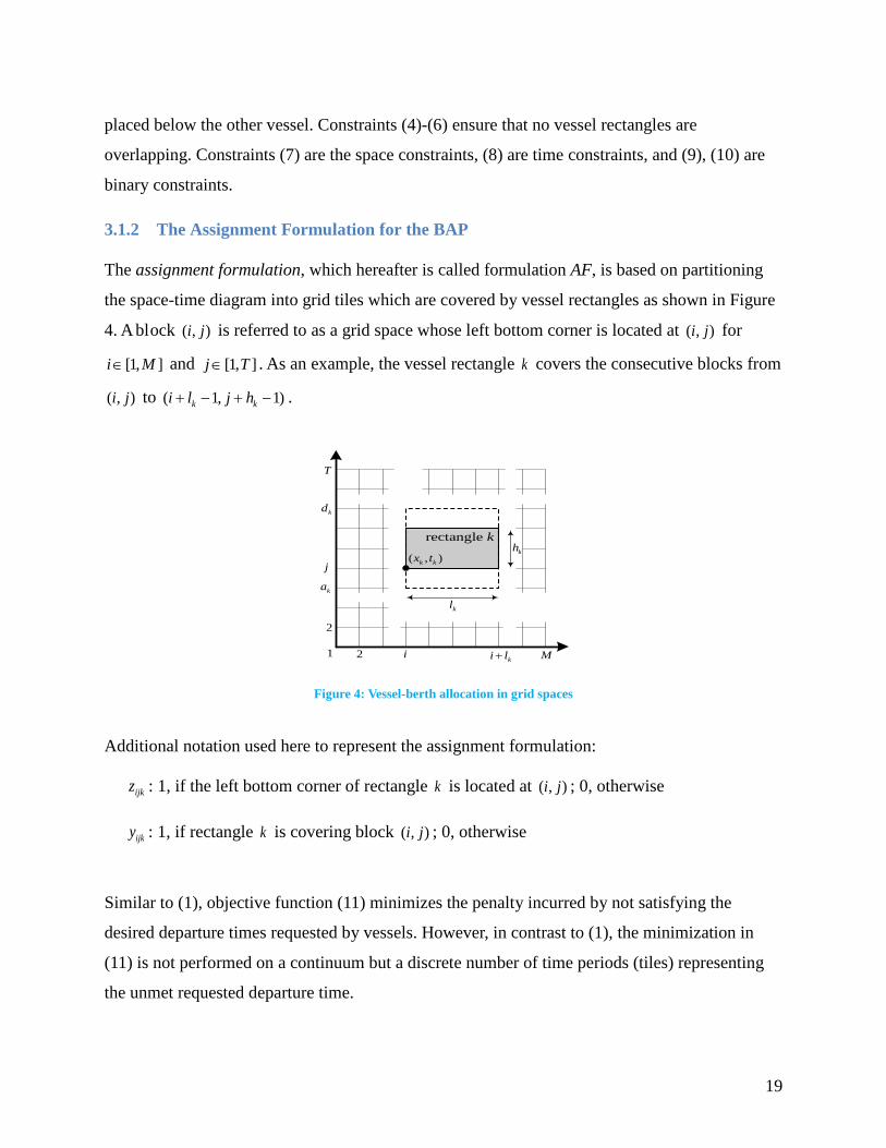
The assignment formulation, which hereafter is called formulation AF, is based on partitioning
the space-time diagram into grid tiles which are covered by vessel rectangles as shown in Figure
4. A block ( , )i j is referred to as a grid space whose left bottom corner is located at ( , )i j for
[1, ]i M∈ and [1, ]j T∈ . As an example, the vessel rectangle k covers the consecutive blocks from
( , )i j to ( 1, 1)k ki l j h+ − + − .
kd
ka
rectangle k
( , )k kx t
i
j
kl
M
T
kh
1 2
2
ki l+
Figure 4: Vessel-berth allocation in grid spaces
Additional notation used here to represent the assignment formulation:
ijkz : 1, if the left bottom corner of rectangle k is located at ( , )i j ; 0, otherwise
ijky : 1, if rectangle k is covering block ( , )i j ; 0, otherwise
Similar to (1), objective function (11) minimizes the penalty incurred by not satisfying the
desired departure times requested by vessels. However, in contrast to (1), the minimization in
(11) is not performed on a continuum but a discrete number of time periods (tiles) representing
the unmet requested departure time.

20
min 1 1
1 1( )
k k
k
M l T hK
ijk k k kk i j a
z w j h d− + − +
+
= = =
⋅ + −∑ ∑ ∑ (11)
s.t. 1
1K
ijkk
y=
≤∑ , i j∀ (12)
1 1
0k ki l j h
ijk k k mnkm i n j
z l h y+ − + −
= =
− ≤∑ ∑ 1, , 1, , , 1, k k ki M l j a T h k∀ = − + = − + (13)
1 1
11
k k
k
M l T h
ijki j a
z− + − +
= =
=∑ ∑ k∀ (14)
{0,1}ijky ∈ , ,i j k∀ (15)
{0,1}ijkz ∈ 1, , 1, 1, , 1, k ki M l j T h k∀ = − + = − + (16)
Constraints (12) imply that a block is covered by at most one vessel rectangle. Constraints (13)
ensure that blocks covered by a vessel rectangle must be consecutive. Constraints (14) imply that
each vessel has only one berthing coordinate. Constraints (15) and (16) are binary constraints.
3.1.3 The Mixed Integer Linear Programming Formulation for the BAP
The following formulation, which hereafter is called formulation MILPF, is equivalent to the
BAP formulation in RPF and is the mixed integer linear programming formulation for the BAP.
Similar to (1), the unmet desired departure times requested by vessels are minimized in (17).
min 1
K
k kk
w β +
=∑ (17)
s.t. k k k k kt h d β β+ −+ − = − k∀ (18)
( ) ( 1) 0l k k klx x l Nα σ− + − − − ≥ , ,k l k l∀ ≠ (19)
( ) ( 1) 0l k k klt t h Nτ δ− + − − − ≥ , ,k l k l∀ ≠ (20)
, 0k kβ β+ − ≥ k∀ (21)
and Constraints (4)-(10).
The objective function in (17) minimizes the penalty cost resulting from the delay in the
departure time of vessels. A method for dealing with ( )k k kt h d ++ − variables is to introduce new
variables kβ+ and kβ
− , constrained to be nonnegative, and let k k k k kt h d β β+ −+ − = − . It is intended to

21
have k k k kt h d β ++ − = or k k k kt h d β −+ − = − , depending on whether k k kt h d+ − is positive or
negative. Then the original problem (RPF) can be formulated as a MILP by adding a
corresponding constraint (18) to (21).
For an optimal solution to the problem, and for each value of k , we must either have 0kβ+ = or
0kβ− = . That is true since otherwise we could have reduced both kβ
+ and kβ− by the same amount
while preserving feasibility. In other words, we could have reduced the cost, which is in
contradiction to optimality. Constraints (19) and (20) are to enforce the definitions of klσ and klδ ,
and N is a large positive number.
3.1.4 Some Notes on Alternative Objective Functions
The objective function used in (1) minimizes the penalty associated with the violation of the
desired departure times requested by the vessels. A generalized alternative for this objective
function is one that rewards early service operations. The following function is a possible choice
for generalized objective function, which is a linear combination of penalized late departure time
and rewarded early service operation.
{ }1 22
1(( ) ) ( ( ))
K
k k k k k k k kk
w t h d w d t h+ +
=
= + − − − +∑J (22)
where 1 0kw > is the penalty weight, and 2 0kw > is the reward weight. We require that 1 2k kw w≥ .
The setback is that 2J may assume both negative and positive values. To make 2J non-negative,
the possible maximum value of the second term is added to 2J as an offset. Hence, a better
choice for the generalized objective function would be
( )1 2 23
1(( ) ) ( ( )) ( ( ))
K
k k k k k k k k k k k kk
w t h d w d t h w d a h+ +
=
= + − − − + + − +∑J . (23)
The objective function 3J can also be rewritten as

22
3
2
1 21
( ), for ( ) 0(( ) ) ( ( )), for ( ) 0
Kk k k k k k
k k k k k k k k k k k k
w t a t h dw t h d w d a h t h d=
− + − <=
+ − + − + + − ≥∑J (24)
3J tries to minimize the delayed departure times while maximizing the temporal margin after
completion of the service. A very interesting special case of 3J - which has been considered by
other researchers [6], [8], is the one in which 1 2k kw w= . This special case will result in
41
1( )
K
k k kk
w t a=
= −∑J (25)
The objective function 4J minimizes the delayed mooring time only. Furthermore, by adding a
fixed offset 1k kw h to 4J , the choice of the objective function will be as follows
( )51 1 1
1 1( ) ( )
K K
k k k k k k k k kk k
w t a w h w t h a= =
= − + = + −∑ ∑J (26)
The objective function 5J minimizes the delayed mooring and handling times. This choice of
objective function was considered by Guan and Cheung [12] and Imai et al. [10].
Figure 5 shows two different final solutions, when 4J or 5J is used. The two solutions are both
optimal if 1kw is the same for all the ships. However, if we consider a more general situation in
which a delayed departure disturbs the successive assignments, the first solution cannot be
optimal. In such a case, we can introduce the generalized objective function and can penalize the
delayed departure time with a higher penalty weight to get an optimal solution.

23
1
2
2a
2d
1a
1d
2
1
1a
1d
2a
2d
Solution 1 Solution 2
Figure 5: Possible optimal solutions under different cost functions
3.2 Solution Methods for the BAP
Since the continuous BAP is an NP-hard problem, in this section, we develop two approximation
methods to find good solutions in a reasonable amount of time. Without loss of generality,
formulation MILPF, described in section 3.1.2, is used to illustrate the solution methods. In the
sequel, we will focus on this formulation.
3.2.1 The Lagrangian Relaxation Method for the BAP
Many hard integer problems can be viewed as an easy problem complicated by a relatively small
set of side constraints. Dualizing side constraints produces a Lagrangian problem which is easy
to solve and whose optimal value is a lower bound for minimization problems on the optimal
value of the original problem. This method was termed “Lagrangian relaxation” by Geoffrion
[20], who developed a systematic methodology to construct the lower bounds as a means of
exploiting special problem structure.
The problem (MILPF) can be converted into a relaxed problem using the Lagrange multipliers
0ijπ ≥ , , i j∀ , as follows:
( )LBz π = 1 1
1 1 1 1 1 1min ( ) 1
k kM l T hK M T K
ijk k k k ij ijkk i j i j k
z w j h d yπ− + − +
+
= = = = = =
⋅ + − + −
∑ ∑ ∑ ∑∑ ∑ ( LRπ )
s.t. Constraints (13)-(16).
where ijπ π = , 1, ,i M= and 1, ,j T= , is a matrix of Lagrange multipliers.
The dual problem of the relaxed problem ( LRπ ) becomes

24
LBz = max ( )LBzπ
π , (D)
where 1 1
1 1 1 1 1 1( ) min ( ) 1
k kM l T hK M T K
LB ijk k k k ij ijkk i j i j k
z z w j h d yπ π− + − +
+
= = = = = =
= ⋅ + − + −
∑ ∑ ∑ ∑∑ ∑
s.t. Constraints (13)-(16), and 0ijπ ≥ .
If we ignore the last constant term in (D), then ( )LBz π is equivalent to
1 1
1 1 1 1 1 1min ( )
k kM l T hK M T K
ijk k k k ij ijkk i j i j k
z w j h d yπ− + − +
+
= = = = = =
⋅ + − +∑ ∑ ∑ ∑∑ ∑ (27)
When 1ijkz = , we have 1ijky = for , , 1km i i l= + − and , , 1kn j j h= + − . Therefore, for a vessel k ,
the second term becomes
1 1
1 1
k ki l j hM T
ij ijk mni j m i n j
yπ π+ − + −
= = = =
=∑∑ ∑ ∑ (28)
Then, this implies that the relaxed problem ( LRπ ) can be considered as
1 1 1 1
1 1 1min ( )
k k k kM l T h i l j hK
ijk k k k mnk i j m i n j
z w j h d π− + − + + − + −
+
= = = = =
+ − +
∑ ∑ ∑ ∑ ∑ (29)
s.t. Constraints (14)-(16)
The solution to ( LRπ ) can be obtained since (29) is separable in k . The optimal coordinate for
each sub-problem is calculated by setting 1ijkz = .
1 1
,min ( )
k k
k
i l j h
k k k mni j a m i n jw j h d π
+ − + −+
≥= =
+ − + ∑ ∑ (30)

25
To optimize dual functions in Lagrangian relaxation, we use the subgradient method (SG) for
separable integer programming problems. All sub-problems are solved optimally to obtain a
subgradient direction. The subgradient method is an adaptation of gradient methods, in which
gradients are replaced by subgradients. For further discussion on subgradient methods see [21].
Given an initial value 0ijπ = , a multiplier is generated by the following rule:
( ){ }1max 0, 1K
ij ij ijkks yπ π
== + −∑ (31)
where ijky is from an optimal solution to ( LRπ ) and s is a positive scalar step size. We use the
following step size which has been commonly adopted in practice [22].
( )
21
( )
|| 1||UB LBK
ijkk
z zs
y
λ π
=
−=
−∑ (32)
where λ is a scalar satisfying 0 2λ< ≤ and UBz is the best known feasible (upper-bound) solution
value obtained by applying a heuristic to formulation (MILPF).
We use a general rule, which is to set 2λ = for some fixed number of iterations. This number is
called maxIter hereafter. At each iteration, we successively halve both the values of λ and
maxIter until the value of maxIter reaches some threshold (here, number 4). Note that,
alternatively, the procedure can be stopped when λ reaches a threshold.
To describe our developed subgradient optimization procedure for the BAP, the following
notation is used.
LBz maximum lower bound from Lagrangian relaxation
UBz minimum upper bound
1Hz initial upper bound found by Heuristic H1 (it is described in section 3.2.3)
2Hz updated upper bound found by Heuristic H2 (it is described in section 3.2.4)
minUB best upper bound so far
maxLB best lower bound so far

26
maxIter maximum number of iterations
The following procedure, named BAPsg procedure, describes our developed subgradient
optimization method.
BAPsg Procedure (Berth Allocation Problem- Subgradient Method)
1. Calculate the initial upper bound using H1, 1UB Hz minUB z= =
Set 0LBz maxLB= = , 2λ = , 0ijπ = , and 2maxIter K=
2. If 0.005λ < , then stop. Otherwise, continue.
3. Update the lower bound LBz .
If LBz maxLB> , then LBmaxLB z= , 2λ = , and 1Iter = . Otherwise, 1Iter Iter= + .
4. Update the minimum upper bound using H2, 2UB Hz z=
If UBz minUB< , then UBminUB z= .
If 0LBz = , then stop. Otherwise, continue.
5. If Iter maxIter> , then 0.5λ λ= × , max{4, 0.5}maxIter maxITer= × , and 1Iter = .
6. Update the step size s and the multiplier ijπ . Go to step 2.
In Step 3 of the BAPsg procedure, the lower bound LBz is acquired by solving each sub-problem
(30). Then, the heuristic H2 is applied to find a feasible solution in Step 4. Details about
heuristics H1 and H2 will be provided in sections 3.2.3 and 3.2.4. In the end, the procedure
returns the best feasible solution (the minimum upper bound) and the maximum lower bound. At
the end of each iteration of the procedure, an optimal solution to (D) may be still infeasible for
(MILPF), which means that vessel rectangles may be overlapping. However, as the multipliers
corresponding to vessels with infeasible berthing are increased, the cost of (D) is increased. This
ensures that the solution associated to LBz gets close to a feasible solution of the original problem
(MILPF).
Figure 6 demonstrates an instance of a BAP with initial and final solutions which were obtained
by the above procedure. In the figure, each batch is represented by a distinct color. A batch is

27
defined as a set of rectangles in the space-time domain, where the sum of their lengths, including
safe distances between them, is less than or equal to the berth length M. The batch concept is
fundamental to our heuristic methods which will be described later. The left figure is a berth
allocation plan represented by color-filled rectangles. The figure on the right shows the
corresponding plan along with time constraints. The time constraints of each vessel are
represented with a dotted rectangle. The height of a dotted rectangle is determined by the vessels’
arrival and desired departure times and the width is equal to the vessel’s length.
If a vessel rectangle is not fully enclosed by its (dotted) constraint rectangle, it will results in a
cost increase. As shown in Figure 6(a), the initial feasible solution indicates that two rectangles
(A and B) are not completely enclosed by their constraint rectangles. Figure 6(b) shows the final
lower bound solution, which is still infeasible, since several rectangles overlap. Finally, the final
upper bound solution is shown in Figure 6(c). In this specific example, the procedure yields an
optimal solution to (MILPF) without penalty cost associated with waiting times.
Various port disruption events can be graphically described by using a vessel rectangle and its
constraint rectangle. The disruption can result in changes to either the vessel rectangle or to the
constraint rectangle. For example: (a) If, because of equipment break-down, the service time kh
is delayed by ω hours, then the height of the vessel rectangle is lengthened by ω hours. That is,
the vessel rectangle could change. (b) If the arrival time ka is delayed by ω hours, because of
delays due to an unexpected event, the constraint rectangle should be adjusted and, also, the
berthing time should be adjusted so that k kt a ω≥ + . That is, both the vessel rectangle and its
constraint rectangle could change.
In both cases above, we can graphically detect whether the changed rectangles (resulting from a
disruptive event) disturb an original allocation plan or not. If the original allocation plan is
disrupted, and the disturbance occurs in batch b , we will reallocate vessel rectangles in the later
batches ( 1, 2,b b+ + ).

28
200 400 600 800 1000 1200
20
40
60
80
100
120
140
160
berth [m]
time
[h]
Initial feasible soultion
200 400 600 800 1000 1200
20
40
60
80
100
120
140
160
berth [m]
time
[h]
Initial feasible soultion with time constraints
(a) Initial feasible solution
200 400 600 800 1000 1200
20
40
60
80
100
120
140
160
berth [m]
time
[h]
Lower bound soultion
200 400 600 800 1000 1200
20
40
60
80
100
120
140
160
berth [m]
time
[h]
Lower bound soultion with time constraints
(b) Lower bound solution (infeasible)
200 400 600 800 1000 1200
20
40
60
80
100
120
140
160
berth [m]
time
[h]
Upper bound soultion
200 400 600 800 1000 1200
20
40
60
80
100
120
140
160
berth [m]
time
[h]
Upper bound soultion with tim constaints
(c) Upper bound solution
Figure 6: Initial and final solutions found by applying subgradient method
3.2.2 The Simulated Annealing Method for the BAP
The second methodology developed is based on simulated annealing (SA) to find good solutions
to the BAP. The SA methodology was independently presented by Kirkpatrick et al. [23] and

29
Cerny [24]. The SA algorithm resembles the annealing process in metallurgy. In each step of the
algorithm, the current state (solution) is replaced, with some probability, by a randomly
generated neighboring state. This probability depends on the difference between the current state
energy (cost) and generated neighbor energy, as well as, on a global parameter T (temperature)
which is gradually decreased using a scheduled parameter r (cooling rate). The SA algorithm is
such that it makes the system ultimately move to lower energy states (called downhill
movements). Also, uphill movements prevent the algorithm from staying at local minima.
Before describing the methodology in detail, we start by defining the variables and parameters,
neighbor search function, and acceptance probability function for our SA procedure.
3.2.2.1 Notation and Definitions
The following notation is used in this section.
sc current state
sn new state
sb best state
ec energy (cost) of current state, ec=E(sc)
en energy of new state, en=E(sn)
eb energy of best state, eb=E(sb)
T0 initial temperature
r cooling rate
3.2.2.2 Neighbor (candidate move) Search Procedure
A new state (solution) sn is obtained by exchanging a pair of consecutive vessel rectangles in the
current state sc . The current state (1, , )sc K= is defined as a sequence of vessel rectangles.
BAPneighbor Procedure
1. Choose a rectangle k , where {1, , 1}k K∈ −
2. Exchange the order of the pair ( , 1)k k + in the current state sc
3. Update to a new state sn by applying heuristics H1 and H2
Details about heuristics H1 and H2 are provided in sections 3.2.3 and 3.2.4.
30
3.2.2.3 Acceptance Probability Function
A probability of making the transition from the current state to a candidate state is specified by
an acceptance probability function. We adopt the following acceptance probability (AP) function,
as described in [23].
( )1,
( , , )exp ( ) / , otherwise
en ecAP ec en T
ec en T<= −
(33)
where parameter T is a designed parameter (temperature in metallurgy).
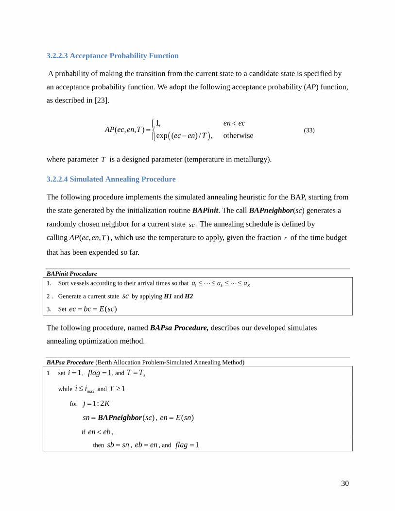
3.2.2.4 Simulated Annealing Procedure
The following procedure implements the simulated annealing heuristic for the BAP, starting from
the state generated by the initialization routine BAPinit. The call BAPneighbor(sc) generates a
randomly chosen neighbor for a current state sc . The annealing schedule is defined by
calling ( , , )AP ec en T , which use the temperature to apply, given the fraction r of the time budget
that has been expended so far.
BAPinit Procedure 1. Sort vessels according to their arrival times so that 1 k Ka a a≤ ≤ ≤ ≤
2 . Generate a current state sc by applying H1 and H2
3. Set ( )ec bc E sc= =
The following procedure, named BAPsa Procedure, describes our developed simulates
annealing optimization method.
BAPsa Procedure (Berth Allocation Problem-Simulated Annealing Method)
1 set 1i = , 1flag = , and 0T T=
while maxi i≤ and 1T ≥
for 1: 2j K=
( )sn sc= BAPneighbor , ( )en E sn=
if en eb< ,
then sb sn= , eb en= , and 1flag =

31
elseif ( , , ) (1)AP ec en T rand> ,
then sc sn= and ec en=
End
End
set T rT=
if 1flag = ,
then 1i i= + and 0flag =
End
End
3.2.2.5 Initial Temperature and Cooling Rate
The choice of the initial temperature T0 and the cooling rate r affects the quality of the solutions
obtained by the simulated annealing procedure. To be able to determine the right values for T0
and r , we generated ten instances of the BAP problem whose size are randomly varied from 16
to 21 vessels. Details about generating an instance of the BAP are given in a later section. Each
BAP was solved 700 times using different combinations of T0 and r . In our experiments, T0 was
varied from 10 to 130 by a step of 10, whereas r was changed from 0.5 to 0.95 by a step of 0.05.
For each T0 and r , the results were averaged and shown in Figure 7.
0 20 40 60 80 100 120 1401.06
1.07
1.08
1.09
1.1
Temperature
Obj
ectiv
e va
lue
Average normalized objective value
0.5 0.55 0.6 0.65 0.7 0.75 0.8 0.85 0.9 0.951.04
1.06
1.08
1.1
1.12
Cooling rate
Obj
ectiv
e va
lue
Figure 7: Normalized objective values
In Figure 7 each normalized value represents the ratio of the corresponding objective value to the
lowest objective value. On average, the minimum objective value was found at the initial

32
temperature 70 and the cooling rate 0.6. These values are used in the succeeding experiments.
Figure 8 shows the average number of iterations to reach final solutions (a) and the number of
minima (b). Note that the minima of each combination were selected over 10 repeated tests as
described above.
As seen from Figure 7, a combination of a higher temperature and a higher cooling rate,
generally, yields better solutions. However, such combination requires higher number of
iterations too, which means more running times. The actual required running time of a certain
combination can be deduced from the figure. It shows that our choice ( 0 70T = and 0.6r = ) needs
less than 300 iterations to reach to final solutions. Also, the quality of solutions with respect to
the parameters can also be estimated from Figure 2.8b. It indicates that our chosen parameters
yield a higher number of minima (about 6.5). Therefore, the chosen parameters are expected to
produce good solutions within reasonable time.
Cooling rate
Tem
pera
ture
Average number of iterations to reach final solutions
0.5 0.55 0.6 0.65 0.7 0.75 0.8 0.85 0.9
20
40
60
80
100
120
180
200
220
240
260
280
300
320
340
Cooling rate
Tem
pera
ture
The number of minimums
0.5 0.55 0.6 0.65 0.7 0.75 0.8 0.85 0.9
20
40
60
80
100
120
3.5
4
4.5
5
5.5
6
6.5
7
7.5
Figure 8: (top) Density plot, showing the average number of iterations to reach final solution;
(Bottom) Number of minima. Both graphs are parameterized by the cooling rate and Temperature.
3.2.3 H1: Heuristic Method for an Initial Feasible Solution
Although methods based on subgradients with Lagrangian relaxation and methods based on
simulated annealing have been used in the literature to solve the BAP and similar allocation
problems, our heuristic procedures are quite different from any procedures reported previously in
the literature. As already mentioned, our heuristics implement a set of systematic and efficient
methods in order to find an initial feasible solution and to update a current solution by exploring

33
a sufficiently large solution space.
To find and update feasible solutions for both subgradient (SG) and Simulated Annealing (SA)
algorithms, two heuristic methods are developed. The first method is called Heuristic H1 and is
developed to generate an initial feasible solution. Using H1, each vessel rectangle is sequentially
placed on the solution space according to its arrival order. Heuristic H2 is developed to
repeatedly improve the feasible solution, using pair-wise swaps between neighboring rectangles
within a batch or over neighboring batches. A batch is defined as a set of rectangles where the
sum of their lengths including safe distances between them is less than or equal to the berth
length M.
Under any combination of rectangle movements and swapping operations, Heuristic H2 tries to
create rooms (temporal spaces) for rectangles to be berthed to the earliest possible time (pushed
down).
3.2.3.1 Algorithm for an Initial Feasible Solution
The following notation is additionally used to describe the heuristic procedures.
pS the set of rectangle indices in a batch p
B the number of batches in a berth, that is p=1,…,B
qp the number of rectangles in a batch p, that is, | |p pS q=
Heuristic Procedure H1 (Algorithm for an initial feasible solution) 1. Construct a batch of rectangles by assigning their berthing locations
set 1 1x = , 1p = , and {1}pS =
for 2 :k K=
1 1k k kx x l α− −= + +
if k kx l M+ ≤ , then p pS S k=
else, 1kx = , 1p p= + , and create { }pS k=
end
2. Assign a feasible berthing time with the earliest possible berthing time
for 1:k K=

34
if 1k S∈ , then k kt a=
else, max{ , }k k s st a t h τ= + + for all 1kps S −∈
end
where 1kpS − is a subset of 1pS − , satisfying s k kx x l α< + + and s s kx l xα+ + > for 1ps S −∈ and
pk S∈ . In other words, s represents a rectangle in 1pS − whose berthing space overlaps with
rectangle k .
3.2.4 H2: Heuristic Method for an Improved Feasible Solution
The heuristics H2 uses a series of rectangle movement functions, which consist of all possible
directional movements and swapping operations. The heuristics H2 procedure is used to improve
an initial feasible solution in the initialization stage and to improve current feasible solutions in
both subgradient (SG) and simulated annealing (SA) procedures for the BAP.
Heuristic Procedure H2 (Algorithm for improving the feasible solution)
1. Set 2Hz with the minimum of known feasible solution value
2. Find 2newHz by running SWAPb, SWAPt, RIGHT, and LEFT
3. Update and return 2Hz if 2 2newH Hz z≤
Given a feasible solution, a slightly different combination of rectangle movements might work
better for some problem instances.
3.2.4.1 Rectangle Movement Operators For the sake of clarity we introduce here the rectangle movement operators. These operators
define all the possible movements of a rectangle in time‐space, and will be the basis of the
rectangle movement functions in the next section.
35
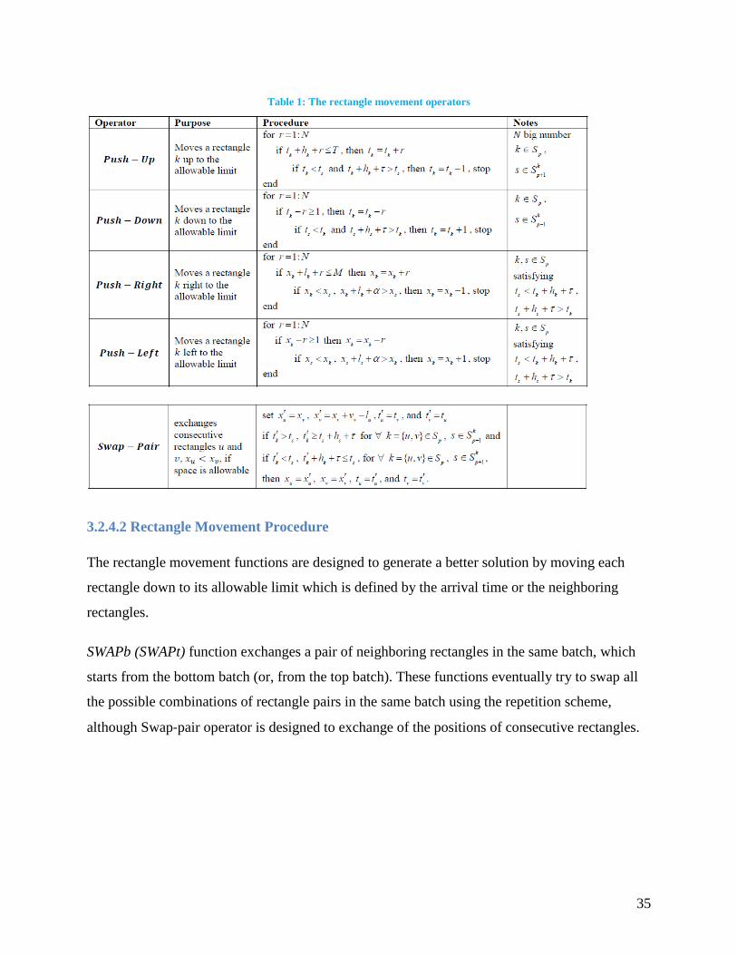
Table 1: The rectangle movement operators
3.2.4.2 Rectangle Movement Procedure The rectangle movement functions are designed to generate a better solution by moving each
rectangle down to its allowable limit which is defined by the arrival time or the neighboring
rectangles.
SWAPb (SWAPt) function exchanges a pair of neighboring rectangles in the same batch, which
starts from the bottom batch (or, from the top batch). These functions eventually try to swap all
the possible combinations of rectangle pairs in the same batch using the repetition scheme,
although Swap‐pair operator is designed to exchange of the positions of consecutive rectangles.

36
SWAPb (SWAPt) Procedure
1. for 1:p P= ( :1p P= )
for 1: 1pq q= −
if p P< , then
Push-Up 1pk S +∈
Swap-Pair q and 1q +
Push-Down 1p pk S S +∈
else
Swap-Pair q and 1q +
Push-Down pk S∈
If the cost increases, then restore their positions
end
end
RIGHT (LEFT) function pushes a rectangle ( )pS q to the allowable limit or to the next nearest
rectangle on the right (or, on the left) in the same batch.
RIGHT (LEFT) Procedure
1. for 1:p P=
for 1pq q= −
if p P< , then
Push-Right q (Push-Left q )
Push-Down 1p pk S S +∈
else
Push-Right q (Push-Left q )
Push-Down pk S∈ . if the cost increases, then restore their positions
end
end
The following figures show how the combination of several rectangle movement functions can
reduce the allocation cost. Each allocation plan for a vessel is represented by a shaded rectangle
along with its arrival time and requested departure time (dotted box). Also, darker shade

37
represents the region which causes a penalty cost due to the violation of the desired departure
time.
( )pS q( 1)pS q+
1( 1)pS q+ ′+1( )pS q+ ′
1( )pS q+ ′
1( 1)pS q+ ′+
( )pS q( 1)pS q+
Figure 9: Reduction by SWAPx resulting from Swap-Pair between Sp(q) and Sp(q+1) followed by Push-Down Sp+1(q’).
( )pS q( 1)pS q+
1( 1)pS q+ ′+
1( )pS q+ ′
( )pS q( 1)pS q+
1( 1)pS q+ ′+
1( )pS q+ ′
Figure 10: Reduction by RIGHT resulting from Push-Right of Sp(q+1) followed by Push-Down Sp+1(q’).
( )pS q
( 1)pS q+
1( 1)pS q+ ′+1( )pS q+ ′
( )pS q
( 1)pS q+
1( 1)pS q+ ′+
1( )pS q+ ′
Figure 11: Reduction by LEFT resulting from Push-Left of Sp(q+1) followed by Push-Down Sp+1(q’+1).
3.3 Computational Experiments for the BAP
A disruption at a berth may result in changes in the space-time diagram as compared to the
baseline plan. The disruption may alter the diagram in the time dimension, the space dimension,
on in both dimensions. Usually, disruptions in the time domain are caused by delayed arrival
times, delayed berthing times, or longer service times. Disruptions in the space domain are less

38
frequent yet their impact is more severe on the port operations. They may be the result of
anticipated events (e.g., construction, scheduled maintenance, pre-planned military surge, etc.),
or unanticipated events (e.g., terrorist acts, earthquakes, hurricanes, etc.).
In this section, we will consider disruptions caused by delays, i.e., disruptions affecting only the
time dimension of the space‐time diagram. Disruptions affecting the space dimension will be
studied in Section 4, where we introduce partially operational berths and the Terminal Allocation
Problem. Here we assume that the delays are caused by an increase in the number of calling
vessels on the berth. This increase in the number of vessels to be serviced could be for example a
direct consequence of physical break‐downs in adjacent berths within the same terminal/port, due
to unanticipated events. Because of the increased number of vessels, we may not be able to serve
all the vessels within their requested time frames. The objective is to minimize the total delay
incurred for all the vessels. We will show, via several computational experiments that our
developed subgradient and simulated annealing optimization techniques will be able to deal with
this type of disruptions by finding the best allocation for the calling vessels such that the total
delay is minimized. The CPLEX MIP solver is used to find exact solutions for small size
problems, enabling us to evaluate the quality of the solutions generated by our methodologies for
such problems.
3.3.1 CPLEX MIP: Computational Experiments
The computational experiments are conducted using realistic data obtained from Park and Kim in
[5], and Kim and Moon in [13]. In order to generate random instances, we use a discrete uniform
distribution whose Cumulative Distribution Function (CDF) is given by
1
1( ; , ) ( )1
n
ii
F x a b H x xb a =
= −− + ∑ (34)
where the Heaviside step function ( )iH x x− is the CDF of the degenerate distribution centered at
ix . Table 2 shows the range of parameters a and b assumed in our simulation experiments to
generate kl , kh , ka , and kd . For instance, kh is generated randomly using the given CDF for
7a = and 23b = . Upon choosing kh , the value of ka is randomly generated using the same CDF
with parameters 1a = and 1kb T h= − + . Note that kd is chosen so that 2k k k kh d a h≤ − ≤ . In our

39
simulation experiments, we set 1200[ ]M m= , 168[ ]T h= , 20[ ]mα = , and 2[ ]hτ = .
Table 2: Ranges of parameters α and b
Parameter kl [m] kh [h] ka [h] kd [h]
a 170 7 1 k ka h+
b 290 23 1kT h− + 2k ka h+
We assume that the weight kw in (1) is equal to the area covered by the vessel rectangle, i.e.,
k k kw l h= ⋅ . This choice of kw imposes higher penalties to be paid to ships with possibly higher
workloads, if the requested departure times are not met.
Using the specifications given in Table 2, we generate 500 random instances of the BAP. Table 3
compares the performance of the CPLEX MIP solver (IP), the subgradient optimization method
(SG), and the simulated annealing method (SA).
Table 3: Comparison between the BAP solutions using IP, SG, and SA methods
K rOC Cost Average time[s] Maximum time[s]
zIP zSG zSA zIP/zSG zIP/zSA tIP tSG tSA mIP mSG mSA
11 0.19 10.7 32.4 14.3 3.03 1.34 0.0 2.0 2.1 10.6 115.4 178.0
12 0.21 23.5 46.7 41.5 1.99 1.77 0.2 3.4 6.6 25.4 130.8 254.1
13 0.22 34.0 112.8 52.8 3.31 1.55 0.8 5.5 8.5 236.5 106.2 252.0
14 0.24 71.2 187.1 115.9 2.63 1.63 1.7 11.2 20.0 468.8 183.8 444.6
15 0.26 89.8 310.0 170.1 3.45 1.89 28.8 13.7 21.5 6781.0 238.1 367.8
16 0.27 89.7 299.2 137.6 3.34 1.53 16.7 19.1 31.0 1486.2 234.2 481.8 17 0.29 230.4 606.4 307.6 2.63 1.33 156.8 30.5 61.8 24739.6 260.4 639.6
18 0.31 244.0 683.4 389.7 2.80 1.60 361.1 38.7 76.9 38798.5 239.3 617.6
In Table 3, IPz , SGz , and SAz are, respectively, the average cost of the best solutions found by the
IP, SG and SA. The average and the maximum running times for different methodologies are also
shown in the table. It indicates that the cost ratio of SA to IP (i.e., /IP SAz z ) is rather small which

40
means that SA yields good quality solutions. The cost ratio /IP SGz z is much higher than /IP SGz z .
To improve the solution quality of SG, one can increase the number of iterations of H2.
The occupation ratio of a berth, denoted by OCr , is defined as the sum of the vessel rectangles
divided by the entire space
1
( )KOC k kk
r h l MT=
=∑ (35)
The occupation ratio is an indicator of the berth utilization. As indicated by Table 3, as OCr
increases, more time is needed to find the best solutions.
As it can be seen from Table 3, the IP can solve the problem instances up to K =18. However,
comparing to the heuristics, as K increases, the IP needs considerable amount of time to find the
exact solution. We noticed that for K >18, we will not be able to find the exact solutions in a
reasonable amount of time. This limitation will be more pronounced as we move toward the
dynamic BAP and the multiple BAP, which are discussed in the following sections.
3.3.2 Heuristic Methods: Computational Experiments
We assume that the number of vessels calling on a berth is between 12 to 20 vessels. This
number is close to the numbers of vessels considered in real‐life scenarios in [5], [13].
In Table 3, we have observed that the exact method is able to find the optimal solution, in a
reasonable amount of time, for K ≤16 . However, the running time of the exact method is
abruptly increased when K ≥17 . In this subsection and in order to evaluate and compare our
developed heuristic methods, we consider instances of the BAPs with 17 ≤ K ≤ 21. We adopt the
generalized objective function J3 in (23) with 1 10k kw l= and 2k kw l= . These values are chosen so
that we can impose higher penalties on delayed departure times. The values of 1kw and 2
kw are
directly proportional to the length of the vessel k, kl . Hence, higher priority is given to larger
vessels which, most probably, carry higher volume of loads.
Table 4 shows the performance of the SG and SA optimization methods over various sizes of
problems. Among randomly generated instances, 20 instances are selected as long as they have a

41
non‐zero initial feasible solution. Each result in the table is averaged over 20 such independent
trials.
Table 4: Performance comparison between SG and SA methods
K rOC Subgradient optimization Simulated Annealing
zSA/zUB zLB zUB gSG tSG cSG zSA tSA cSA
17 0.29 145.2 380.3 1.6 590.4 227.1 322.1 133.3 148.1 0.85
18 0.32 403.2 737.4 0.8 742.5 281.6 532.8 183.1 195.4 0.72
19 0.33 525.8 897.9 0.7 711.0 268.6 569.3 154.7 183.4 0.63
20 0.35 428.6 899.7 1.1 845.4 304.8 545.9 261.1 289.0 0.61
21 0.36 729.5 1951.2 1.7 822.8 268.6 1409.1 248.5 261.4 0.72
In the table 4, OCr is the occupation ratio of a berth, LBz is the maximum lower bound from
Lagrangian relaxation model, UBz is the minimum upper bound (best feasible solution by the SG
method), SGg is the duality gap between LBz and UBz , defined as ( ) /SG UB LB LBg z z z= − , SGt is the
computational time of the SG method, SGc is the number of iterations of H2 in the SG method,
SAz is the best feasible solution by the SA method, SAt is the computational time of the SA
method, and SAc is the number of iterations of H2 in the SA method. The duality gap SGg implies
the maximum deviation of the final lower bound from the best feasible objective value. The
duality gap ranges from 70% to 170% which means that the SG produces good approximations
of optimal solutions.
In Table 4, in order to improve the solution quality of the SG methodology, we may increase the
number of iterations of H2. It is noted that step 4 in BAPsg doesn’t need to be executed every
iteration. We noted that the step should be executed when LBz maxLB< or LBz maxLB≤ .
We can also observe that, on the average, the SA algorithm still yields a non-inferior solution,
which ranges from 61% to 85% of the corresponding upper bound found by the SG algorithm.
This might have resulted from the fact that the range for swapping operations in the SA method
is little wider. Considering the superiority of the solution quality and the running time of the SA

42
methodology, in the following sections we will only use the SA methodology to find the best
solutions to other variants of the BAP namely the dynamic BAP, and multiple BAP.
4 Terminal Allocation Problem (TAP)
Usually certain berthing locations (home berths) are preferred due to the long-term contracts
with carriers, the depth of water, differing wave heights, etc [5]. In this section, we assume that
for some predicted or unpredicted scenarios (disruptions) a calling vessel cannot moor at its
home berth location and that other berth locations (within the same terminal or adjacent
terminals) can accommodate the vessel. This leads to a more complex, yet general, variant of the
BAP which, hereafter, is referred to as the terminal allocation problem (TAP).
In the TAP, we assume that we have N disjoint berths. The disjoint berths could belong to the
same or to different terminals, and because they are disjoint, a vessel can utilize only one such
berth (i.e. a vessel cannot moor across two or more such berths). The disjoint property will
enable us to model a partially functional terminal (e.g., a terminal consisting of N disjoint berths,
of which 1N N≤ have been rendered non functional due a disruptive event, hence there are only
1N N− remaining functional berths). We assume that the length of berth n is nM and that the
time horizon for all berths is T . Figure 12 illustrates the TAP graphically in a space-time
diagram.
T
1MBerth 1
Time
T
2MBerth 2
T
NMBerth N
•••
Figure 12: Space-time diagram for the Terminal Allocation Problem
The TAP can be stated as follows: Determine the least-cost assignment of K vessels to N
disjoint berths such that each vessel is assigned to exactly one berth and no two vessels are

43
overlapping (in the space-time domain), while all the vessels’ constraints (arrival times, service
times, etc.) are met. Therefore, the TAP consists of two intertwined problems: (1) A set
partitioning problem (SPP), and (2) A number of individual berth allocation problems (BAPs).
4.1 Set Partitioning Problem
Given a collection of feasible subsets of a certain ground set, one can formulate the problem of
finding the best collection of subsets such that the cost associated with these subsets is
minimized. This problem is called the set partitioning problem (SPP).
Let jy be 1 if berth j is functional and at least one vessel is assigned to it, and zero otherwise.
Let jc be the cost of berth j which is computed as the aggregated costs of serving all the vessels
assigned to that berth. Let also ija be 1 if vessel i is assigned to berth j , and zero otherwise. The
SPP can be formulated as follows:
min 1
N
j jj
c y=∑ (36)
s.t. 1
1N
ij jj
a y=
=∑ , 1, ,i K= (37)
{0,1}jy ∈ , 1, ,j N= (38)
Almost every heuristic approach, for solving general integer programming problems, has been
considered and applied to the set partitioning problem. For instance, in [15], some greedy
algorithms and interchange approaches were applied to the SPP problem. Other heuristic
approaches such as genetic algorithms; probabilistic search, simulated annealing, and neural
networks have also been studied and applied to the problem. In addition, heuristics are embedded
within exact algorithms so that one iteratively tightens the upper bound and at the same time
attempting to get a tight approximation to the lower bound for the problem [16], [17].
Unfortunately, there has not been a comprehensive and comparative test across such methods to
determine under what circumstances a specific method might perform best.
It should be noted that the SPP is known to be NP-hard [19]. As described above, the TAP can be

44
mapped into the SPP; hence, the TAP is an NP-hard problem too. Moreover, the TAP consists of
a collection of BAPs, where each BAP is an NP-hard problem [7].Therefore, as the number of
the berths and vessels in the TAP increases, finding an optimal solution will be computationally
too expensive. In the following, we develop an approximation methodology to find good
solutions to the TAP in a reasonable amount of time.
4.2 Solution Method for the TAP
Figure 13 demonstrates our approach toward the TAP. The approach is based on a typical set
partitioning procedure. Assuming that the terminal consists of N disjoint berths, the TAP is
partitioned into N BAPs. Each BAP is solved separately using the previously developed
heuristics H1 and H2 as described before. Based on our computational results and findings
presented in Section 3.3, we will use the simulated annealing methodology for each BAP
sub‐problem.
Figure 13: The TAP as a set partitioning problem
Initially, a specific number of vessels, calling on the port is assigned to each berth. This number
is proportional to the area of the space‐time diagram of each berth. If a vessel has specifically
requested to be served at a particular berth, it will be assigned to that berth, unless other
restrictions at the berth prohibited this assignment.
Recall from Section 3.1.2 that a block ( , )i j is referred to as a grid space whose left bottom

45
corner is located at the point ( , )i j . The overlapping value of block ( , )i j at berth n , denoted by
ijnc , is defined as the number of overlapping vessels at block ( , )i j at that berth. The maximum of
this value is { }max, ,maxn ijni j
c c= , 1, , ni M= and 1, ,j T= .
Let Bn be the set of vessels assigned to berth n. Assume vessel k The vessel k overlapping
index, denoted by kIV , is defined as the number of blocks whose values are max,nc within the
vessel rectangle k . The overlapping index of berth n , denoted by nIB , is defined as the sum of
the block values in that berth.
1 1
nM T
n ijni j
IB c= =
=∑∑ (39)
Figure 14 illustrates a simple example to demonstrate how to find a vessel’s and a berth’s
overlapping indices. The right figure shows berth n containing two overlapping vessel rectangles
k and k ′ . For this example max, 1nc = , 2nIB = , and 2k kIV IV ′= = .
0 0
000
0
00
0000
110
0 0 0 0
ka
kt
kdk
k′
Figure 14: Value of the block
Before describing the SA methodology for the TAP in details, we define the variables and
parameters used in our SA methodology.
4.2.1 Notations and Definitions
A vessel rectangle k, denoted by kv , is defined by a 9‐tuple as follows.
( )1 2, , , , , , , ,k k k k k k k k k kv n l h a d w w x t= (40)
where

46
kn is the assigned berth index for vessel rectangle k
kl is the length of vessel k
kh is the estimated handling time of vessel k
ka is the estimated arrival time of vessel k
kd is the requested departure time of vessel k
1kw is the penalty weight assigned to vessel k
2kw is the reward weight assigned to vessel k
kx is the assigned mooring location to vessel k
kt is the assigned mooring time to vessel k
Let nB be the set of vessels assigned to berth n . That is,
( ){ } { }| , , , , 1, , , 1, ,n k k k k kv v n t n n k K n N= = = = ∈ B (41)
where K is the number of vessels to be scheduled, and n nK=B is the cardinality of the set
representing the number of vessels assigned to berth n . A state s is formed by aggregating all nB
in a single set, i.e.
{ }1, , N=s B B . (42)
The cost of the state s is defined as the sum of the costs of all the individual berths nB forming s .
Recall that the cost of each berth is defined in (1). Alternative costs were discussed in 3.1.4.
In addition, the following notation is defined and used in this section. sc current state
sn new state
sb best state
ec cost of the current state sc , ( )E=ec sc en cost of the newt state sn , ( )E=en sn eb cost of the best state sb , ( )E=eb sb In the set partitioning algorithm, we construct a single aggregated state sc to easily perform an
interchange operation. The new state sn is obtained from the current state sc by exchanging a

47
pair of vessel rectangles across different berths. After interchanging vessels across different
berths, the optimization procedure is sequentially applied to the sub-problems. Each sub‐problem
by itself is a BAP. The BAP optimization algorithms were discussed extensively in the previous
section. The policy for choosing the pair of vessels to be exchanged is represented in lines 2 to 5
of the following procedure.
NewPartition 1. Order the rectangles of a current state sc by arrival times.
2. Choose (randomly when tie) a berth 1b having max nIB .
3. Choose (randomly when tie) a vessel 1k having max kIV where 1bk∈B .
4. Choose the first 2k such that 1 2k ka a< and
1 2k kn n≠ .
5. If 2k cannot be found, go to step 2
Else, exchange the berth indices of 1kv and
2kv .
6. Divide into sub-states { }|n k kv n n′ = =B and sort by arrival times.
7. Generate an initial solution for each BAP by applying H1 and H2.
8. Update each state ( )n n′= BAPsaB B and return a new state { }1, , N=sn B B .
4.2.2 TAP Procedure
The proposed solution procedure for the TAP is referred to as TAPproc. In the procedure, the
sum of nIB s under i th partition is denoted by isIB (line 3 in the following procedure description).
This procedure is terminated when the best objective function value of the TAP or the sum of the
berth overlapping indices isIB reaches zero (line5).

48
TAPproc (Terminal Allocation Problem Procedure) 1. Initialize =bc sc by TAPinit, ( )E= =eb ec sc , 1i = , and 0r = .
2. while maxi i≤
3. ( )=sn scNewPartition , ( )E=en sn , and i nnsIB IB=∑
4. if <en eb , then =sb sn and =eb en ;
5. if 0=eb or 0isIB = , then stop
6. for 1: 1j i= −
7. if j isIB sIB= , then 1r r= +
8. End
9. if maxr r= , then stop
10. End
The TAP optimization algorithm starts by a feasible solution generated by TAPinit. Vessels are
alternately assigned to berths according to their arrival times. However, in the presence of a
partially functional berth (which will be defined later), the initial subsets will be assigned based
on the ratio of the operational region in the space-time domain.
TAPinit 1. Sort the order of rectangles of a current state sc by arrival times
2. Assign a berth index to each vessel (mod )kn k N≡
3. Divide into sub-states ( )|n k kv n n′ = =B
4. Generate an initial solution by applying H1 and H2
5. Update each state ( )n n′= BAPsaB B
4.3 Port Disruptions Resulting in Partially Functional Berths
A berth is said to be functional (or fully functional) if the entire berth is available to be used by
the calling vessels for the entire planning horizon. A berth is partially functional if some sections
along the berth are not operational for some periods of time. These non‐operational regions may
be caused by anticipated events (e.g. construction; scheduled maintenance; pre‐planned military
surge etc.), or by unanticipated disruptions (e.g. terrorist acts; earthquakes; hurricanes etc.).

49
Recall that a port disruption will result in changes of the space‐time diagram as compared to the
baseline plan. A partial region in the space‐time diagram is termed a cell. A non‐operational
region is regarded as a cell termed a non‐operational cell. The remaining region in the
space‐time diagram can be divided into several operational cells based on its shape. These cells
are all mutually disjoint and exhaustively cover the space‐time diagram. Figure 15 illustrates the
space‐time diagrams for three different examples of partially functional berths.
To decompose the time‐space diagram into operational and non‐operational cells, we can employ
a simple coverage type algorithm [18]. This is similar to grid‐based coverage algorithms used in
mobile robot applications, such as demining, lawn mowing, and floor cleaning tasks. These
algorithms require complete coverage of an unstructured environment with obstacle avoidance.
Our non operational regions in the space‐time domain are comparable to obstacles in the mobile
robot applications. Both our operational non‐operational regions are rectangular in shape, hence
we can easily employ a grid-based coverage algorithm.
Subsequently, our developed heuristics are modified to incorporate the terminal allocation
problem when a berth is only partially functional. A cellular decomposition scheme is
incorporated into the heuristic H1, which was developed to generate an initial feasible solution.
The modified heuristic is referred to as heuristic mH1. Once the vessels are assigned to batches,
heuristic H2 will be deployed to improve the current solution. Recall that a batch is defined as a
set of rectangles where the sum of their lengths including safe distances between them is less
than or equal to the berth length M. The cellular decomposition scheme is done in two stages in
the modified heuristics. At first, the solution space is roughly decomposed into cells that allow
some overlapping with neighboring operational cells. Figure 15 shows some examples of the
decomposed cells from the first stage. The space-time diagrams are divided into several
operational and non-operational cells. The cells are mutually disjoint and exhaustively covering
the space-time diagram. An operational cell r is defined by the coordinate of its lower-left
corner and the projected distances of its upper-right corner along both axes: ( , , ,r r r rx t M T ), where
the total number of operational cells is R , i.e., |r|=R

50
1M 2M
1T
2T
Operational cell 1
Operational cell 2
Non-operational
cell
M
T
1
2
M
T
2
3
1Non-
operational cell
Non-operational
cell
1
2
1 1 1 1( , , , )x t M T11x
Figure 15: Examples of partially functional berths
In the second stage, any overlapping is removed since the upper cells are adjusted by the
allocation plan of lower cells. Then, the cells are mutually disjoint and exhaustively cover the
solution domain. In the modified procedure for an initial feasible solution, the cells are
decomposed and allocated in two stages by the following procedure in a bottom-up fashion.

51
Heuristic procedure, mH1 (Algorithm to generate an initial feasible solution for TAP)
where 1kpS − is a subset of 1pS − , satisfying s k kx x l α< + + and s s kx l xα+ + > for 1ps S −∈ and
pk S∈ .
In lines 4-9, each batch of rectangles is constructed by assigning their berthing locations. The
first rectangle of operational cell r is denoted as rk and is allocated at the beginning section of
the cell, rx . In lines 10-13, a feasible berthing time is assigned as the earliest possible berthing
time. Finally, in lines 14-18, a batch that overrides with the next cell is determined as the last
batch of the current cell. The contour of the next cell is adjusted according to the allocation plan
of the current cell. Eventually, the entire functional region can be decomposed into independent
cells occupied by a feasible berthing plan. If an overlapping takes place in the last batch, it
implies that the remnant of the current scheduling will stay for the next planning horizon.

52
However, in a rolling horizon framework, we can easily generate a feasible solution by
considering the next planning horizon as a neighboring cell.
The contour of the next cell is adjusted according to the allocation plan of the current cell.
Eventually, the entire functional region can be decomposed into independent cells occupied by a
feasible berthing plan, as shown in Figure 16.
Figure 16: Allocation on decomposed operational cells
By repeatedly applying the steps used in H1, this modified procedure generates an initial feasible
solution when a non‐operational cell exists in a berth space‐time domain.
Therefore, in the case of a partially functional berth, the heuristic mH1 replaces H1 in
procedures BAPneighbor, BAPinit, and BAPsa. Subsequently, the procedures for the mBAP
should be properly modified to handle a situation where a partially functional berth exists among
multiple berths. We assume that all ships can be allocated to any berth, possibly, allowing for
extra penalty if the ship does not moor at its home berth. Again, in the presence of a partially
functional berth, the heuristic mH1 replaces H1 in the procedure NewPartition.
In particular, vessel rectangles are distributed according to the proper occupation ratio in the
initialization procedure, which is referred to as mTAPinit.
In the presence of a non-operational region, the occupation ratio of berth n , ( )OCr n , is redefined
as the sum of the vessel rectangles and the non-operational area of nA divided by the entire space.

53
( ) ( )( )k n
OC k k n nk vr n h l A M T
∈= +∑ B
(43)
mTAPinit 1. Sort a current state { }1, , N=sc B B by arrival times
2. Assign a berth index to each vessel: (mod )kn k N≡ 3. Randomly substitute berth indices so that
( )1
1 ( )1 ( )
OCn N
OCn
r nK Kr n
=
−=
−∑ where
1
Nnn
K K=
=∑
Divide into sub-states { }|n k kv n n′ = =B
4. Generate a feasible solution by applying mH1 and H2
5. Update each state ( )n n′= BAPsaB B
4.4 Computational Experiments for the TAP
In this section, we perform several computational experiments are performed to evaluate our
developed methodology for the TAP. Our computational experiments consist of both functional
and partially functional berths. Here, we consider vessels with both flexible and inflexible
berthing locations and departure times. To evaluate our develop techniques, under different
experimental scenarios, we use the cost function 6J defined as
36 3
1min
K
k k kk
w n m=
= + −
∑J J , (44)
where 3J is the cost function defined in (23), km the desired (home) berth location for vessel k ,
and 3kw the spatial penalty for vessel k . The penalty 3
kw is applied to a vessel which cannot be
moored at its desired berth. The last term in 6J , in fact, penalizes the difference between the
assigned and the desired berthing location for vessel k .
In our computational experiments, and without loss of generality, we assume the following
values for wk1,wk
2 and wk3.
54
1 , if 1 and 10 , otherwise
dk k k k
kk
Q f t h dw
l = + >=
2k kw l= (45)
3 , if 1 and 2 , otherwise.
bk k k
kk
Q f n mw
l = ≠=
where Q is a big positive real number
1, if the departure time of vessel is not flexible0, otherwise
dk
kf
=
(46)
1, if the berthing location of vessel is not flexible0, otherwise
bk
kf
=
In the following, we will consider various scenarios to evaluate our developed methodologies
under different circumstances.
4.4.1 Case I: Vessels with Flexible Berthing Locations and Departure Times
Here, we assume that the calling vessels have flexible berthing locations and flexible departure
times (i.e., 0dkf = and 0b
kf = ). By flexible berthing locations, we mean that the vessels do not
have any restrictions on the section of the berth they will be assigned to. However, these vessels
may be willing to moor at any other berth within the terminal or may only choose a specific berth.
In our experiments, and without loss of generality, we assume that 3N = , 1200nM M m= = for
1, ,3n = , and 168T h= . We also assume that the number of vessels mooring at each berth is
initially uniformly distributed between 16 to 21.
Scenario 1: In this scenario, all three berths are functional and the vessels are not flexible to
change their berths. In fact, this scenario can be viewed as three disjoint BAPs.
Scenario 2: In this scenario, the vessels in Scenario 1 are flexible in changing their berths. This
scenario, in fact, represents an instance of the TAP with three berths.
We randomly generated 20 instances of the problem are randomly generated with general
specifications as described above. Each instance is comprised of three BAPs such that at least
one BAP has a non-zero cost (i.e., the value of the objective function generated by H1 is non-

55
zero).
In order to evaluate the proposed heuristics for Scenarios 1 (BAPs) and 2 (TAP), a series of
BAPprocs and TAPproc are successively applied to each instance. The results are averaged and
summarized in Table 5.
Table 5: Experiment results for Scenarios 1 and 2
rOC Scenario 1 Scenario 2
g12 zS1 tS1 cS1 zS2 tS2 cS2 pS2 0.31 2796.0 967.7 491.8 27.3 7700.7 4558.0 13.5 0.99
In Table 5, OCr is the occupation ratio of the terminal which is defined as the statistical mean of
( )OCr n in (41). Siz is the value of the best solution in Scenario i , Sit the computational time in
seconds, Sic the number of iterations of procedure H2 by calling BAPneighbor, Sip the number
of iterations of the set partitioning by calling NewPartition, and ijg the cost reduction as a
solution gap between Scenarios i and j , i.e., ( ) /ij Si Sj Sig z z z= − .
As seen from the table, due to the flexibility of vessels in choosing different berths, the total
allocation cost of Scenario 2 is reduced by 99% (g12=0.99) compared to Scenario 1. The table also
shows that the running time for scenario 2 is almost 8 times larger than that of scenario 1.
The following scenarios 3 and 4, are similar to scenarios 1 and 2, under the additional condition
that one of the berths in the terminal is now only partially functional.
Scenario 3: Consider Scenario 1 again. Here, berths 2 and 3 are fully functional while berth 1 is
partially functional. We assume that berth 1 has a non-operational cell between 600-1200m in
space and 1-100h in time in the space-time diagram.
Scenario 4: Consider Scenario 2 again. Similar to Scenario 3, we assume that berths 2 and 3 are
fully functional while berth 1 is non-operational between 600-1200m in space and 1-100h in time.
Using the same problem instances generated for Scenarios 1 and 2, Scenarios 3 and 4 are created
by assuming a non-operational cell in first berth, respectively.

56
Table 6 summarizes the average results over 20 problem instances, Comparing Table 6 and Table
5, we can easily observe that the non-operational cell increases the occupation ratio from 0.31 to
0.41 and it increases the cost of BAPs by more than 10 times. It indicates that, even in the
presence of a partially functional berth, the allocation cost can still be reduced by using multiple
berths. It is found that the cost is decreased by 93% (g12=0.99).
Table 6: Experiment results for Scenarios 3 and 4
rOC Scenario 3 Scenario 4
g34 zS3 tS3 cS3 zS4 tS4 cS4 pS4 0.41 32232.0 1241.0 504.8 2266.8 41036.8 26338.5 44.7 0.93
4.4.2 Case II: Vessels with Strict Berthing Locations and Departure Times
Hence, we assume that the departure times and/or the berthing locations of some vessels cannot
be violated (i.e., 1dkf = and/or 1b
kf = for some vessels). Accordingly, the set of vessel rectangle
kv assigned to berth n , nB , is divided into two subsets:
( ){ }( ){ } { }
| , , , , 0, 1, , , and
| , , , , 1, 1, , 1, ,
free bn k k k k k k
fixed bn k k k k k k
v v n t n n f k K
v v n t n n f k K n N
= = = = =
= = = = = ∈
B
B (47)
The procedures for generating an initial feasible solution and an updated partition are
respectively modified to handle the inflexible requests by vessels. First the rectangles from the
first subsequence freenB are distributed over N berths according to the initial occupation ratio
( )OCr n and then the assigned rectangles are combined with the rectangles from the second set fixed
nB .
In the set partitioning procedure NewPartition, only the rectangles from the set freenB are selected
for swapping operation. The following four scenarios 5‐8 are used to evaluate the proposed
algorithms when some vessels have requested strict berthing locations and departure times.
Scenario 5: We assume that all three berths are functional and that vessels are not flexible in
changing their berths. Additionally, we assume that 30% of the vessels in each berth have strict
departure time requests. In fact, this scenario represents three BAPs having strict berthing time

57
requests.
Scenario 6: In this scenario, we assume that some vessels in Scenario 5 are flexible in changing
their assigned berths, However, 30% of the vessels in each berth have requested strict berth
location. In fact, this scenario represents a TAP having strict requests on berthing times and
berthing locations.
Again, we randomly generated 20 instances. Each instance is comprised of three BAPs such that
at least one BAP has a non-zero initial objective function value generated by H1. In order to
evaluate the proposed heuristics over scenarios 5 (BAP) and 6 (TAP), a series of BAPprocs and
TAPproc are successively applied to each instance. The averaged results are summarized in
Table 7.
Since the BAPs in Scenario 5 have the strict requests on departure times, some vessels’
rectangles, probably with lower priority, may not be allocated in the current time horizon
(possibly placed over two consecutive planning horizons). The number of these undesirable
allocations in Scenario i is denoted by Sie .
According to the results, if vessels are allocated to the single integrated terminal with multiple
berths, the allocation cost can be reduced by 63% even with the strict requests on berthing
locations and departure times. Note that the average number of vessels having the inflexible
departure times is 5.55 for 3 berths. These vessels having higher priority could make some
allocations undesirable. However, by implementing the TAP, the number of undesirable
allocations can also be reduced from 0.27 to 0.09. Table 7 also shows that the running time is
increased from 0.19 to 2.24 hour.
Table 7: Experiment results for Scenarios 5 and 6
rOC Scenario 5 Scenario 6
g56 zS5 tS5 cS5 eS5 zS6 tS6 cS6 pS6 eS6 0.31 31258.1 666.4 489.9 0.27 11442.2 8052.1 6916.6 10.8 0.09 0.63
Furthermore, additional scenarios are prepared to compare the BAPs and TAP in the presence of
a partially functional berth. Using the same problem instances generated for scenarios 5 and 6,

58
scenarios 7 and 8 are prepared by adding a non-operational cell in the first berth, respectively.
Scenario 7: Consider Scenario 5 again. Assume that berth 1 has a non-operational cell between
600-1200m in space and 1-100h in time while berths 2 and 3 are fully functional.
Scenario 8: Consider Scenario 6 again. Similar to Scenario 7, we assume that berths 2 and 3 are
fully functional while berth 1 has a non-operational cell between 600-12000m in space and 1-
100h in time.
Table 8 shows the benefit of implementing the single integrated terminal in the presence of a
partially functional berth when vessels have both strict requests on berthing locations and
departure times.
A comparison between Table 6 and Table 7 indicates that, although the presence of the non-
operational cell increases the cost of BAPs by more than 700%, the allocation cost is still
reduced to 57%. In addition, the number of undesirable allocations is reduced from 1.91 to 0.82,
on average. Table 8 also shows that the running time is increased from 0.24 to 6.03 hours.
Table 8: Experiment results for Scenarios 7 and 8
rOC Scenario 7 Scenario 8
g78 zS7 tS7 cS7 eS7 zS8 tS8 cS8 pS8 eS8 0.41 221176.1 872.3 599.2 1.91 95818.3 21724.5 21444.5 33.5 0.82 0.57
5 Disruption Mitigation at the Regional Level
Logistics service providers or carriers consolidate their freight in a network of hubs and
terminals and build up regular services. The design of such services requires decisions about the
frequency, mode, and route of the service and the corresponding schedule and routing of freight.
Planning decisions for such networks are made on a tactical level and have a direct impact on
customer services and costs. These kinds of tactical planning problems are generally referred as a
service network design [25].
5.1 Service Network Design
Railways, less-than-truckload (LTL) motor carriers, mail/package delivery services, airlines,

59
intermodal shipping lines are typical examples of such systems that require tactical planning of
operations. Service network design is increasingly used to designate the set of main tactical
issues and decisions relevant to the described carriers: the selection and scheduling of the
services to operate, the specification of the terminal operations, the routing of freight, the empty
balancing strategy, etc. The corresponding models usually takes the form of network design
formulations, a class of the mixed-integer network optimization problems for which no efficient
exact solution method exists, except for special variants [26].
In this section, we describe a general service network design problem containing decisions
regarding the service selection and the traffic distribution. In the service selection, the routes
which services are offered and the characteristics of services are defined. In the traffic
distribution, the paths between origins and destinations are determined to move every demand.
Network design formulations are defined on graphs containing nodes connected by links. The
objective is to select links in a network, along with capacities, eventually, in order to satisfy the
demand for transportation at the lowest possible system cost computed as the total fixed cost of
the selected links, plus the total variable cost of using the network. Consider a graph
( , )=G N A which represents a physical network, where N is a set of node and A is a set of
links.
FORMULATION FCSN. The following formulation, which hereafter is called formulation
FCSN, is equivalent to the fixed cost service network.
Min ( , ) ( , ) ( , )
p pij ij ij ij
i j i j i jf y c x
∈ ∈ ∈
+∑ ∑ ∑A A P
(48)
Subject to p p pij ji i
j jx x d
∈ ∈
− =∑ ∑N N
i∈N , p∈P (49)
pij ij ij
px u y
∈
≤∑P
( , )i j ∈A (50)
0pijx ≥ ( , )i j ∈A , p∈P (51)

60
{0,1,2, }ijy ∈ ( , )i j ∈A (52)
where
• ijf is the fixed cost incurred by opening service on link ( , )i j per service unit
• ijy is the discrete decision variable which represents the number of service units (e.g.
trucks) offered on link ( , )i j
• pijc is the transportation cost per unit flow of product p on link ( , )i j
• pijx is the flow decision variable indicating the amount of flow of commodity p using
link ( , )i j
• pid is the demand of product p at node i
• iju is the capacity of link ( , )i j .
The objective function (48) minimizes
the cost of all relevant decisions, i.e., the service selection and the traffic distribution. Constraint
(49) is the flow conservation and demand satisfaction requirements. Constraint (50) is the capaci
ty restriction of the flow on each link. Constraints (51) and (52) ensure the variables are nonnega
tive and the design variable is an integer.
5.2 Service Network for the U.S. West Coast Region
The focus area for developing mitigation strategies at the regional level, is the region consisting
of the entire west coast of the United States. The region contains multiple marine ports and the
associated ground transportation network, through which goods move within the region and in
and out of the region. The basic question at the regional level is: “what is the impact of
appropriate mitigation measures if one of the ports in the region becomes partially or fully non-
functional for a specific period of time?”
The existing service network is defined at a high level of aggregation, which includes the major
ports and aggregated terminals (zones) representing broad geographical destinations and

61
intermediary terminals. To define the regional network at an appropriate level of resolution, the
2002 Origin-Destination data from the Freight Analysis Framework (FAF) of U.S. DoT FHWA
(Federal Highway Administration) is used [27]. Using the FAF data, the service network of the
west coast region, including the state of Nevada, is constructed. This region consists of 11 zones.
In addition, the remainder of the U.S. is considered as one zone and four major combined ports
(Los Angeles and long beach, San Francisco, Portland, and Seattle) are also added in the network.
Then, the regional service network consists of 20 nodes as shown in Figure 17. The zoning of the
FAF is represented in Figure 17(a) and the corresponding network is shown in Figure 17(b).
109
85
9
8
12
59
60
11
10
84
110
POo
West Coast
SEi
R
SEo
SAo
LAo
POi
SAi
LAi
O ZI
(a) FAF’s zoning (b) constructed network
Figure 17: Service network for the U.S. west coast region
Sine each zone in the FAF data represents an aggregated location of demands, it is modeled as a
node ( ZN ). A port of disembarkation is not represented as a zone in the data. However, each port
node is added to supply the zones. Also, in order to assign the capacity to a port node, it is split
into an inbound node ( IN ) and outbound node ( ON ). In this level of aggregation, a link does not
imply a specific freeway or railway between two corresponding nodes. Rather, it represents an

62
aggregated path by possible ground transportation modes (trucks and trains). This distribution
network for import freight is assumed to handle an aggregated single commodity. Then, N is a
set of node comprised of port nodes and zone nodes ( I O Z= ∪ ∪N N N N ) and A is a set of
links comprised of port and ground links ( P G= ∪A A A ),
where, {( , ) | , }P I Oi j i j= ∈ ∈A N N and {( , ) | , , , }G O Z Zi j i j i j= ∈ ∈ ≠A N N N
Formulation MCFP. If all links are activated to move freight, the regional service network can
be modeled as a minimum cost flow problem, which hereafter is called formulation MCFP, is
showed in the following:
Min ( , )
ij iji j
c x∈∑
A (53)
Subject to ij ji ij j
x x d∈ ∈
− =∑ ∑N N
i∈N (54)
ij ijx u≤ ( , )i j ∈A (55)
0ijx ≥ ( , )i j ∈A (56)
where
• ijc is the transportation cost per unit flow in link ( , )i j
• ijx is the flow decision variable indicating the amount of flow using link ( , )i j
• id is the demand at node i
• iju is the capacity of link ( , )i j
Classical pseudopolynomial-time algorithms, such as, cycle-canceling, primal-dual, out-of-kilter,
and relaxation algorithms can be applied to solve this problem. These algorithms have some
commonalities in that they all repeatedly solve shortest path problem. They frequently provide
the essential building blocks and core ideas used in more efficient algorithms. Also, it can be

63
solved by a linear programming method. Note that a linear program with 0-1 incident matrix can
be transformed into a minimum cost flow problem [28].
5.3 Mitigating Disruptions at Regional Level
When a disruption occurs at the regional level, the regional service network may need to be
reconfigured. For example, consider the U.S. west coast region presented in Figure 17. If the LA
port node is rendered non-functional for a period of time, all services originating from the node
will either be discontinued or be operated at lower capacity. The reconfiguration of the service
network is performed by installing a sea transportation mode between ports. Figure 18 shows the
possible sea transportation links (dotted arrows) from the LA port node to other port nodes.
14
13
6
5
9
10
11
8
7
12
15
3
West Coast
20
16
4
2
1
19
18
17
O ZI
Figure 18: Reconfiguration of the regional service network
The choice of sea transportation links will determined by an optimization procedure, which
minimizes a generalized cost while satisfying the transportation demands. Our solution provides
the data about the amount of goods that can be distributed by sea links and the corresponding
alternative ground links. Due to capacity constraints of links, some amounts of goods may not be

64
distributed although all the available sea links are activated. The amount of goods may remains
at the disruptive port waiting to be distributed in the next planning horizon.
Formulation MCFPB. The set of links A are differentiated into port operation links PA , ground
transportation links GA and sea transportation links SA , where, {( , ) | , , }S I Ii j i j i j= ∈ ∈ ≠A N N .
Then, the service network formulation which can mitigate disruptions is modeled as a minimum
cost flow problem with binary constraints. The following formulation is called formulation
MCFPB.
Min ( , ) ( , )S
ij ij ij iji j i j
f y c x∈ ∈
+∑ ∑A A
(57)
Subject to ij ji ij j
x x d∈ ∈
− =∑ ∑N N
i∈N (58)
ij ij ijx u y≤ ( , ) Si j ∈A (59)
ij ijx u≤ ( , ) ,P Gi j ∈A A (60)
0ijx ≥ ( , )i j ∈A (61)
{0,1}ijy ∈ ( , ) Si j ∈A (62)
where
• ijf is the activation cost of sea link ( , )i j
• ijy is the discrete decision variable of sea link ( , )i j
• ijc is the transportation cost per unit flow in link ( , )i j
• ijx is the flow decision variable indicating the amount of flow using link ( , )i j
• id is the demand at node i

65
• iju is the capacity of link ( , )i j
If the maximum flow saturates all the links from the source, the minimum cost flow problem is
feasible. That is to say, when the supplies/demands at the nodes satisfy the condition 0iid
∈=∑ N
,
the minimum cost flow problem has a feasible solution. To make this problem feasible by
ensuring 0iid
∈=∑ N
, we add a set of slack transportation links between port-inbound nodes and
zone nodes. The set of slack transportation links defined as {( , ) | , }K I Gi j i j= ∈ ∈A N N . Then, the
set of links are redefined as P G S K= ∪ ∪ ∪A A A A A . These slack links will provides information
how much of goods cannot be delivered to each demand nodes.
FORMULATION SSST. Formulation (MCFPB) can also be rewritten by separating the set of
slack transportation links and in that case it will be called formulation SSST.
Min ( , ) ( , ) , , ( , )S P G S K
ij ij ij ij ij iji j i j i j
f y c x xω∈ ∈ ∈
+ +∑ ∑ ∑A A A A A
(63)
Subject to ij ji ij j
x x d∈ ∈
− =∑ ∑N N
i∈N (64)
ij ij ijx u y≤ ( , ) Si j ∈A (65)
ij ijx u≤ ( , ) , ,P G Ki j ∈A A A (66)
0ijx ≥ ( , )i j ∈A (67)
{0,1,2, }ijy ∈ ( , ) Si j ∈A (68)
where ijω is the penalty to undistributed goods which could be greater than the cost related to the
alternative sea link choice.
This problem is solved by a branch-and-bound (B&B) method and a linear programming (LP)
relaxation is performed on every leaf of the branch-and-bound tree. The Simplex algorithm is
applied to solve the relaxed LP problem. The Simplex algorithm is defined by the pivot rule. This

66
rule defines the way that decides with vertex of polyhedron is selected when there are many
basic feasible solutions (BFSs) to choose from [29]. Suppose that the pivot rule is always to
move the adjacent to BFS which there is at least increase in the objective function value. Under
this pivoting rule, the Simplex algorithm requires 2 1n − pivoting steps before terminating. More
precisely, in a standard form, the time complexity of LP is ( 2 ) ( 2 ) (2 )n n nO mn O n O= = where,
m is the number of rows and n is the number of columns of the incident matrix. In a worst case,
since a B&B could generate all leafs on the tree and it solves a relaxed LP on every leaf, it takes
exponential time ( ( 1) 2 )naO p p⋅ − ⋅ to solve our problem, where ap the number of ports in
which activated sea links are originated and p is the number of all ports in the network.
As described above, the Simplex algorithm has exponential time complexity. Its average
behavior and worst case behavior have been studied and explained by Borgwardt [30] and Klee
and Minty [31], respectively. There is no deterministic pivot rule under which the Simplex
algorithm is known to take a sub-exponential number of iterations. However, the numerical
behavior is conflict with theoretical analysis [32]. That means that it is efficient in practice, while
having no polynomial time worst-case complexity, although there are no satisfactory theoretical
explanations of its excellent performance. Therefore, the running time in solving our problem is
governed by the term ( 1)ap p⋅ − .
The B&B method explores the set of feasible integer solutions. However, it uses bounds on the
optimal cost to avoid exploring certain part of the feasible set. The developed algorithm follows
the typical B&B strategies, with few implementation strategies which are listed below.
- It always branches a non-convergent sub-problem unless it is a leaf of the B&B tree.
- To break a sub-problem, it chooses a variable ix which is not integer and creates two sub-
problems by adding either of the constraints *i ix x ≤ or *
i ix x ≥ .
- The lower bound of the optimal cost of a sub-problem is obtained by the linear programming
relaxation using the simplex method.
- The upper bound is updated with the best feasible integer solution so far.

67
- As a way of choosing an active sub-problem, it uses depth-first search with back-tracking.
5.4 Computational Experiments
As we described earlier, our regional service network is constructed based on zoning and data
from 2002 FAF. The service network of the US west coast region including the state of Nevada is
constructed, which consists of 11 zones for the interested region, 1 zone for the remainder of the
US, and four imaginary zones for the major combined port areas (Los Angeles, San Francisco,
Portland, and Seattle). In order to assign the capacity to a port zone, each port node is split into
an inbound node and outbound node. Therefore, the regional service network consists of 20
nodes as shown in Figure 18.
The freight demands (in tons) are extracted from multi-dimensional matrices which consist of
origin, destination, commodity, mode, and port of disembarkation. Originally, origins and
destinations consist of 114 regions and 7 international regions. We extracted the freight from the
international regions to the interested ports in the west coast regions. Among all freight, we
selected freight whose transportation modes are truck, train, and a combination of truck and train.
Based on this information, the west coast service network is constructed as shown in Figure 18
and the corresponding demands are defined in Table 9.

68
Table 9: Import Freight Distribution (ton/day) via Major West Coast Ports
node z8 z9 z10 z11 z12 z59 z60 z84 z85 z109 z110 zR Supply
LA 113667 5651 444 2457 4926 1369 61 239 159 757 233 12969 142932
SA 385 8 454 10508 1112 24 59 32 26 76 68 681 13433
PO 321 44 58 34 120 3 25 6643 661 526 1325 935 10695
SE 710 3 31 77 83 1 1 994 670 21861 2525 2819 29775
It summarizes the supplies and demands of four independent distribution networks originating ea
ch combined port complex. First column represents ports of the west coast region and first row re
present zones in the region. Columns 2 to 13 represent demand XXid of zone i supplied by port X
X, independently. Then, LA SA PO SEi i i i id d d d d= − − − − . The last column represents the supply to each
port. Following table describes the legends and indices used in above table and figures.
Table 10: Legends and numbers of nodes describing FAF zones

69
Legend FAF acronym Zone Node
LA CA Los A Los Angeles/Long Beach port areas 17, 1
SA CA San J Oakland port area 18, 2
PO OR Portl Portland port area 19, 3
SE WA Seatt Seattle/Tacoma port areas 20, 4
z8 CA Los A Los Angeles-Long Beach-Riverside, CA 5
z9 CA San D San Diego-Carlsbad-San Marcos, CA 6
z10 CA Sacra Sacramento-Arden-Arcade-Truckee, CA-NV 7
z11 CA San J San Jose-San Francisco-Oakland, CA 8
z12 CA rem Remainder of California 9
z59 NV Las V Las Vegas-Paradise-Pahrump, NV 10
z60 NV rem Remainder of NV 11
z84 OR Portl Portland-Vancouver-Beaverton, OR-WA 12
z85 OR rem Remainder of Oregon 13
z109 WA Seatt Seattle-Tacoma-Olympia, WA 14
z110 WA rem Remainder of Washington 15
zR - Remainder of West Coast Zone 16
The activation cost ijf of link ( , ) Si j ∈A can be defined by ‘the running cost’ of a ship during the
entire trip including the loading at Ii∈N , and the unloading at Ij∈N . The transportation cost
ijc of link ( , ) Si j ∈A is defined as ‘the price per ton’ since the distance is already considered in
the opening cost. Following relations are used to calculate the opening cost and transportation
cost of sea links, especially from LA to other ports.

70
Fuel cost (FC) = (Loading and Unloading time)×Fuel per day at port + Transit time×Fuel per day at
sea
Running Cost = Daily running cost×Total time + fuel cost + port cost
Price per ton = (Daily profit×Total times + Running Cost) / Total tons
Besides the distance information between port nodes, several assumptions are made to calculate
these costs in Table 11.
- Average ship speed is 25 knot.
Transit time (17-18) = 368/25/24 = 0.6133 hour
- Loading/unloading time is 1 hour.
- Fuel consumption per day at port and at sea is 2 ton and 34 ton, respectively.
- Fuel price per ton is $100.
Fuel cost (17-18) = (1×2+0.6×34)×100 = 2240
- Daily running cost of a ship is $5000 and each port cost is $3000.
Activation cost (17-18) = 5000×2.6+2240+3000×2 = 21240 = f17,18
- Daily profit required is $1000.
- Maximum load of a ship is $10000.
Price per ton (17-18) = (1000×2.6+21240)/10000 = 2.384 = c17,18
Table 11: Activation and transportation cost of sea links

71
Sea link Distance Transit time activation
cost Price per ton
i-j (nautical miles)
(h) fij cij
17-18 368 0.6 21240 2.384
17-19 976 1.7 25480 2.818
17-20 1127 1.9 27160 3.006
According to [33], the price per ton-mile of ground transportation modes (truck and train) is
roughly 22 times higher than that of sea transportation mode. Since our price per-tone mile of sea
links is about $0.004, we can proportionally assumed that the price per ton-mile of our ground
transportation link is about $0.1. Then, the ground transportation cost per unit ton is 0.1ij ijc m= ,
where ijm is distance in miles of link ( , ) Gi j ∈A .
The maximum capacity of link is assumed to be high enough to distribute current demands found
in the FAF data. First, the maximum capacity of port link ( , ) Pi j ∈A is defined by increasing the
current optimal flow which is an optimal solution to (MCFP).
* /mij ij pu x r= , (69)
Where, miju is the maximum capacity, *
ijx is the optimal solution to (MCFP), and pr represents
the capacity utilization ratio ( 0 1pr< ≤ ). Without any disruption, a higher pr is given to the LA
port node. However, we will generate a disruption in LA node by reducing it’s pr in the
experiments.
Table 12 shows the maximum capacity of each link and the residual capacity riju which will be
used in PART I of the experiments, later.
Table 12: Estimating capacity (ton) of port links

72
Port Link Optimal flow rp Maximum
capacity
Residual
capacity
17-1 142932 0.9 158813 158813
18-2 13433 0.5 26866 13433
19-3 10695 0.5 21390 10695
20-4 29775 0.6 49625 19850
Secondly, the capacity of ground link ( , ) Gi j ∈A is defined by increasing the current optimal flow
which is an optimal solution to (MCFP).
* /mij ij gu x r= , (70)
where miju is the maximum capacity, *
ijx is optimal solution to (MCFP), and gr represents the
capacity utilization ratio. A higher gr is given to links whose destination has more demand as
shown in Table 13.
Table 13: Estimating capacity of ground links
Zone rg Links
LA Metropolitan area 0.9 1-5,1-6
Other Metropolitan area 0.6 2-7,2-8,3-12,3-14,4-12,4-14
Other than above 0.5 Other than above
5.4.1 Distributions of Freight from LA Port Node
In this part, it is assumed that, if some of freight which cannot be processed in the LA node, they

73
are distributed through other port nodes. Therefore, higher priority is given to the supplies of
those nodes. That is, the distributions between the other nodes to zones are performed a priori.
That is, rij iju u= for ( , ) Pi j ∈A and m
ij iju u= for ( , ) Gi j ∈A . Assume that a disruption occurs in LA
port. As a result of the disruption, we assume that the capacity of link 17-1 is reduced from 90%
to 70% in 5% decrements. Table 14 shows the performance of our mitigation strategy
summarized in terms of the cost of distribution and the amount of remaining freight.
Table 14: Freight distribution from LA port by activating sea links
Capacity Capacity Base Case (MCFP) Reconfiguration Case (SSST)
(%) (ton) RGoods Cost (LA) SA PO SE RGoods Total
Cost
90 142932 0 3.53e+6 2962 1388 0 0 3.36e+6
85 134991 7941 1.91e+6 6457 1484 0 0 3.42e+6
80 127050 15882 6.74e+5 6457 4658 4767 0 3.61e+6
75 119110 23822 5.11e+5 6457 8499 6101 2765 3.78e+6
70 111169 31763 4.45e+5 6457 8499 6101 10706 3.72e+6
The first column represents the current capacity of LA port link with respect to the maximum
capacity. The second column shows the corresponding capacity in tonnage. Cost (LA) is the
optimal cost of distributed goods supplied to the LA node. RGoods is the amount of remaining
goods at LA node due to capacity insufficiency of the overall service network. Suppose that the
optimal solution to (MCFPB) or (SSST) is * *( , )ij ijx y . Then,
* *( , ) ( , ) , ,
PCostS P G S
ij ij ij iji j i jf y c x
∈ ∈= +∑ ∑A A A A
. (71)
*RGoods , ( , )ij Kx i j= ∈A (72)
When the current capacity is down to 90%, all the freight from LA node can be distributed using

74
only ground links. However, by activating two sea links, the computational result indicate that
the distribution cost originating LA node can be further reduced under our assumptions regarding
costs. If the current capacity of LA node is reduced to less than 90%, the part of freight supplied
to LA node cannot be distributed in (MCFP). When the capacity is reduced to 85% or 80%, the
freight supplied to LA zone can still be distributed by opening some of the sea links in (MCFPB).
However, if the capacity of LA node is reduced to 75%, we have excess freight of 2765 ton even
though all the possible sea links from LA are activated.
6 Overall Disruption Modeling and Mitigation
Mitigation strategies have been developed at the terminal, port and regional levels and several
scenarios were discussed to demonstrate the best mitigation strategies to be followed at each
level. It is important that these strategies be integrated with each other, in order to optimize the
routing of ships, trucks and trains and to dissipate the disturbance caused by a disruption at any
level.
Our overall methodology is developed based on minimizing the total cost at all levels. The
regional level takes inputs from the terminal and port levels and the results are used as a new
input to the port level using heuristic methods to optimize the routing of goods to their
destinations as explained in detail in previous chapters. In the following, a computational
experiment is discussed to evaluate the overall methodology applied to a combination disruptions
at all levels.
In the following scenario, we have focused on the port of LA/LB which consists of 15 container
terminals and the adjacent road network. A major portion of the goods from the port complex are
delivered to zone 8 which includes the Los Angeles, Long Beach and Riverside regions. Trucks
take I-710, I-110, 47 and 103 roads to distribute the goods in zone 8 as shown in the Figure 19.

75
Figure 19: Port (LA/LB) complex and adjacent road network.
For the simulation of cargo movements inside terminals we use the macroscopic terminal model
TermSim that was developed under a previous METRANS project and was modified to handle di
sruptions under this project. For the simulation of traffic flow i
n the road network adjacent to the twin ports we use the commercial software VISSIM to develo
p and tune a microscopic traffic simulation model.
The VISSIM based microscopic traffic simulation model is integrated with the macroscopic term
inal model in order to calculate the number of trucks entering and leaving the terminals.
Locations of terminals are shown in Figure 20 and the capacity of each terminal is presented in
Table 15.

76
Figure 20: Location of container terminals

77
Table 15: Capacity of terminals
Terminal# Normal Capacity
(ton/day)
Maximum Capacity
1 11149 6133
2 8290 9133
3 15437 17106
4 7004 7809
5 4145 4609
6 12578 13871
7 4145 4626
8 28015 32150
9 13864 17220
10 8290 12010
11 5717 6985
12 4145 6100
13 5717 7810
14 11149 14905
15 2287 2536
Baseline traffic flow on the adjacent roads prior to applying the scenario assumptions is shown in
Figure 21.

78
Figure 21: Baseline traffic flow
(PCU -Passenger Car Unit, 1 truck=2.5 PCU, 1 car=1 PCU)
In our disruption scenario terminals 1, 2, 3 and 4 are partially functional due to a military surge
(the disruption scenario assumes that the terminals operate at 50% capacity). Therefore, 21100
ton/day is left to be redistributed to the other terminals.
In the following, we provide a comparison of using our methodology, i.e. a combination of the
terminal allocation problem (TAP) and service network optimization, versus separately
optimizing each one.
6.1 TAP and Service Network Optimization (separately)
In this part, the goods are distributed among other terminals. Table 16 shows the performance of
TAP mitigation strategy summarized in terms of distribution of goods in terminals.

79
Table 16: TAP optimization, container distribution
Terminal# Normal Capacity
Maximum Capacity
1 5575 6133
2 4151 9133
3 7775 17106
4 3549 7809
5 4332 4609
6 12803 13871
7 4362 4626
8 32115 32150
9 16467 17220
10 11096 12010
11 8642 6985
12 6085 6100
13 7785 7810
14 14746 14905
15 2501 2536
Figure 22 shows traffic flow in the adjacent network. Traffic congestion is observable in I-110
and 47 highways.

80
Figure 22: Service network optimization, traffic flow
6.2 Combination of TAP and Service Network Optimization
In this part, the impact of the adjacent road network traffic is added to the cost function. As a res
ult, terminals 2 to 8 receive more containers compared to the previous part to relieve the traffic fl
ow on I-110. This is shown in Table 17.

81
Table 17: Combined optimization, container distribution
Terminal# Normal Capacity
Maximum Capacity
1 5575 6133
2 4151 9133
3 7775 17106
4 3549 7809
5 6190 4609
6 14621 13871
7 6297 4626
8 29921 32150
9 15674 17220
10 10009 12010
11 7514 6985
12 5075 6100
13 7514 7810
14 12963 14905
15 4311 2536
As an outcome of considering service network optimization and TAP, the traffic flow shown in
Figure 23 is less congested than traffic flow of Section 6.1.

82
Figure 23: Combined optimization, traffic flow
Figure above demonstrates the improvement of the traffic flow in the network and the total travel
time is reduced by using the combined optimization.

83
7 Conclusions Shipping is the heart of the global economy, but it is vulnerable to disruptions. Disruptions at
marine terminals and ports may cause long delays and long queues at the terminals which may
have enormous adverse impacts on the economy. Disruptions may be the result of anticipated
events (e.g., construction, scheduled maintenance, pre‐planned military surge, etc.), or
unanticipated events (e.g., terrorist acts, earthquakes, hurricanes, etc.). In this project, we
developed strategies to mitigate the effects of such anticipated or unanticipated disruptions in an
effort to maintain port operations and productivity. We investigated methods of modeling and
evaluating port disruptions, at the terminal, port and regional levels.
At the terminal level disruptions were analyzed within the framework of the Berth Allocation
Problem (BAP). Since the BAP, which can be viewed as a rectangle packing problem, is an NP
hard problem, two heuristic optimization techniques based on the sub gradient (SG) and
simulated annealing (SA) optimization methods were developed. Simulation results show that
the developed methodologies are able to find a near‐optimal solution in a reasonable amount of
time.
At the port level the disruptions were analyzed within the framework of a Terminal Allocation
Problem (TAP). In the TAP, vessels calling on a port were represented by rectangles in the
space‐time diagram. Disruptions may alter the diagram in the time, space, or both time and space
domains. Usually, disruptions in the time domain are caused by the delays in arrival times,
delays in berthing times, longer service times, etc. Disruptions in the space domain are less
frequent yet their impacts are more severe on the port operations. They may be caused by
construction, scheduled maintenance, military surge, terrorist acts, etc. When a disruptive event
occurs at a berth, other berths within the terminal may be utilized to further mitigate the impact
of that event. To be able to consider a very general TAP, we defined concepts such as a partially
functional berth which can be used to represents any type of disruptions in the space‐time
diagram. We show that the TAP can be viewed as a set partitioning problem, in which each

84
partitioned problem is a BAP. Since the TAP is also an NP hard problem, a heuristic method
based on the simulated annealing algorithm was developed to find a good solution in a
reasonable amount of time. Numerous experimental scenarios were developed to evaluate the
developed TAP solution method in the presence of disruptions. We show that when multiple
berths are utilized to accommodate calling ships, the impact of disruptions, either anticipated or
unanticipated, can be mitigated significantly using the developed methodologies.
At the regional level disruptions were analyzed within the framework of a service network. The
service network optimization is modeled as a minimum cost flow problem with binary (or,
integer) constraints. Computational experiments showed that the possible cost reduction acquired
under the maximum utilization of the network capacity. The focus was on the entire west coast
region of the US, consisting of multiple ports and the associated transportation network. The
regional service network is defined at a high level of aggregation. Under a disruptive event, the
network is reconfigured by opening sea transportation mode between ports.
In the combined methodology (TAP and service network optimization), the traffic flow in the
road network adjacent to the port is less affected by the disruption in one terminal or multiple
terminals. The road network in Figure 23 shows less traffic congestion in the area and as the
result the total travel time is reduced. Therefore, the total cost is decreased by considering the
combination of disruption mitigation methodologies at all levels.

85
References [1] White House Publication, “The National Strategy for Maritime Security,” http://www.whitehouse.gov/homeland/maritime‐security.html, September 2005. [2] Coulter, D.Y., “Globalization of Maritime Commerce: The Rise of Hub Ports,” in
Globalization and Maritime Power, Edited by Sam J Tangredi, Institute for National Strategic Studies, Dec. 2002.
[3] American Association of Port Authorities, AAPA, http://www.aapaports. org/pdf/NORTH_AMERICAN_CONTAINER_SUMMARY_2003.xls. [4] Long Beach Press Telegram, Sep 6, 2004. [5] K. T. Park, K. H. Kim, “Berth scheduling for container terminals by using a sub-gradient optimization technique,” Journal of the Operational Research Society, vol. 53, no. 9, pp. 1054‐1062, 2002. [6] R. Moorthy and C‐P. Teo, “Berth management in container terminal: the template design problem,” OR Spectrum, vol. 28, no. 4, pp. 485‐518, 2006. [7] J.‐F. Cordeau, G. Laporte, P. Legato, and L. Moccia, “Models and Tabu Search heuristics for the Berth‐Allocation Problem,” Transportation Science, vol. 30, no. 4, pp. 526‐538, Nov. 2005. [8] A. Imai, X. Sun, E. Nishimura, and S. Papadimitriou, “Berth allocation in a container port: using a continuous location space approach,” Transportation Research Part B, vol. 39, no. 3, pp. 199‐221, 2005. [9] A. Imai , E. Nishimura, M. Hattori, and S. Papadimitriou, “Berth allocation at indented berths for mega‐containerships,” European Journal of Operational Research, 179, pp. 579–593, 2007. [10] A. Imai, E. Nishimura, and S. Papadimitriou, “The dynamic berth allocation problem for a container port,” Transportation Research Part B, vol. 35, no. 4, pp. 401‐417, 2001. [11] A. Imai, E. Nishimura, and S. Papadimitriou, “Berth allocation with service priority, “Transportation Research Part B, vol. 37, no. 5, pp. 437‐457, 2003.

86
[12] Y. Guan and R. Cheung, “The berth allocation problem: models and solution methods,” OR Spectrum, vol. 26, no. 1, pp. 75‐92, 2004. [13] K. H. Kim and K. C. Moon, “Berth scheduling by simulated annealing,” Transportation Research Part B, vol. 37, no. 6, pp. 541‐560, 2003. [14] M. Golias, S. Theofanis S., and M. Boile, “Berth and quay crane scheduling: a formulation reflecting start and finish service deadlines and productivity agreement.” Presented at the 2nd Annual National Urban Freight Conference, Long Beach, CA, December 2007. [15] M. Fisher and L. Wolsey, “On the Greedy Heuristic for Covering and Packing Problems,” SIAM Journal on Algebraic and Discrete Methods, vol. 3, no. 4, pp. 584‐591, 1982. [16] K. L. Hoffman and M. Padberg, “Solving Airline Crew Scheduling Problems by Branch and Cut,”Management Science, vol. 39, no. 6, pp. 657‐682, 1993. [17] E. Balas and M. C. Carrera, “A Dynamic Subgradient‐based Branch‐and‐Bound Procedure for Set Covering,” Operations Research, vol. 44, no. 6, pp. 875‐890, 1996. [18] E. González, M. Alarcón, P. Aristizábal, and C. Parra, “BSA: A Coverage Algorithm,” Proc. IEEE‐IROS 2003, pp. 1679‐1684, 2003. [19] M. R. Garey and D. S. Johnson, Computers and Intractability: A Guide to the Theory of NPCompleteness, Freeman, San Francisco, CA, 1979. [20] A. M. Geoffrion, “Lagrangian relaxation for and its uses in integer programming,” Mathematical Programming Study, vol. 2, pp. 82‐114, 1974. [21] M. Held, P. Wolfe, and H. D. Crowder, “Validation of subgradient optimization, Mathematical Programming,” vol. 6, pp. 62‐88, 1974. [22] M. L. Fisher, “The Lagrangian relaxation method for solving integer programming problems,”Management Science, vol. 27, no. 1, pp. 1‐18, 1981. [23] S. Kirkpatrick, C. D. Gelatt, and M. P. Vecchi, “Optimization by Simulated Annealing,” Science, New Series, vol. 23, no. 4598, pp. 671‐680, 1983. [24] V. Cerrny, “A thermodynamical approach to the travelling salesman problem: an Efficient simulation algorithm,” Journal of Optimization Theory and Applications, vol. 45, pp. 41‐51, 1985.

87
[25] N. Wieberneit, “Service network design for freight transportation: a review,” OR Spectrum, vol. 30, no. 1, pp. 77-112, 2007.
[26] T. G. Crainic, “Service network design in freight transportation,” European Journal of Operations Research, vol. 122, pp. 272-288, 2000.
[27] Freight Analysis Framework (FAF), U.S. DoT FHWA, 2002.
http://ops.fhwa.dot.gov/freight/freight_analysis/faf/index.htm
[28] R. K. Ahuja, T. L. Magnanti, and J. B. Orlin, Network flows: Theory, algorithms, and applications, Prentice-Hall, New Jersey, 2003.
[29] G. B. Dantzig, Linear Programming and Extensions, Princeton University Press, Princeton, 1963.
[30] K. H. Borgwardt, The Simplex Method: A Probabilistic Analysis, Berlin:
Springer–Verlag, Heidelberg, 1987.
[31] V. Klee and G. J. Minty, “How good is the Simplex algorithm?” in Inequalities III (Edited by O.Shisha), Academic Press, New York, pp. 159-175, 1972.
[32] R. Shamir, “The efficiency of the simplex method: A survey,” Management
Science, vol. 33, no. 3, pp. 301-334, 1987.
[33] RITA, Bureau of Transportation Statistics, 2009.
https://www.bts.gov/publications/national_transportation_statistics/index.html