Recovery of Chromaticity Image Free from Shadows via Illumination InvarianceMark S. Drew

School of Computing ScienceSimon Fraser University

Vancouver, British ColumbiaCanada V5A 1S6mark@cs.sfu.ca

Graham D. Finlayson and Steven D. HordleySchool of Information SystemsThe University of East Anglia

Norwich,England NR4 7TJ

{graham, steve}@sys.uea.ac.uk

ICCV’03 Workshop on Color and Photometric Methods in Computer Vision, Nice, France, pp. 32-39

Abstract

A recent method for recovering a greyscale image that isfree from shadow effects is extended such that the recoveredimage is a colour image, in the sense that 2-dimensionalchromaticity information is recovered. First, the effect oflighting change, and thus to a large degree shadowing, isremoved by projecting logarithms of 2D colour band-ratiochromaticities into a direction that is independent of light-ing change. The resulting 2-vector colour does not con-tain the contribution of the original lighting in the input im-age, so this is restored by considering the chromaticity forbright pixels. The resulting image is improved by regressionof the chromaticity onto the original image, with promisingresults.

1. IntroductionRecently a new image processing procedure was devisedfor creating an illumination-invariant image from an inputcolour image [1, 2, 3]. Illumination conditions confoundmany computer vision algorithms. In particular, shadowsin an image can cause segmentation, tracking, or recogni-tion algorithms to fail. An illumination-invariant image isof great utility in a wide range of problems in both computervision and computer graphics.

An interesting feature of this problem is thatshadowsare approximately but accurately described as a change oflighting. Hence, it is possible to cast the problem of remov-ing shadows from images into an equivalent statement aboutremoving (and possibly later restoring) the effects of light-ing in imagery. Although shadow removal is not alwaysperfect, the effect of shadows is so greatly attenuated thatmany algorithms can easily benefit from the new method;e.g., a shadow-free active contour based tracking methodshows that the snake can without difficulty follow an object

and not its shadow, using the new approach to illuminationcolour invariance [4].

In the shadow removal method devised, a 3-band colourimage is processed to locate, and subsequently removeshadows. In the original method [1], the output of the al-gorithm is a greyscale image. Although shadows have beenremoved, so too has colour. In [3], colour is put back via us-ing the shadow-free image to guide integrating edges fromthe input colour image. Here, we mean to extend the sim-pler method [1] from greyscale output to output which ispartially colour, in that we recover 2-dimensional colour,along a 1D curve, in the form ofchromaticityρ , defined as[5]

ρ = {r, g, b} ≡ {R, G, B}/(R + G + B) (1)

Although not a full-colour result, as in [3], 2D colour in theform of chromaticity is still useful. To begin with, for aLambertian surface chromaticity removes shading and in-tensity from images. That is, a shaded sphere, say, willappear as a disk. This can lead to images that seem some-what surprising, since they convey colour information only.For example, a crumpled piece of paper in Fig. 1(a), withshading, is reduced to colour-only information in Fig. 1(b).Firstly, since the paper colour, the background, and theblack ink all have approximately the same chromaticity(e.g., forR = G = B, the chromaticity is{1/3,1/3,1/3}) theblack letters recede from our attention; on the other hand,inks that differ only by brightness are now seen as havingthe same essential colour information.

Recovery of the chromaticity is a useful computer vi-sion task, in and of itself, and that is the task we addresshere. By the definition of chromaticityρ in eq. (1), we seethat the chromaticity is not true colour, but is in fact just2-dimensional since the components ofρ are not indepen-dent:

3∑k=1

ρk = 1 (2)

Here we mean to extend the illumination invariant image

32

(a) (b)

Figure 1: 3D colour versus 2D chromaticity.

from 1D greyscale, as in [1], to the type of 2D colour imagein Fig. 1(b).

The method in [1] is in essence a kind of calibrationscheme for a particular colour camera. A camera is cal-ibrated by imaging a (colorful) target, under several dif-ferent illuminants. An invariant image is derived based onthe idea that under Planckian lighting, and for camera sen-sors that are more or less narrowband (as for an ideal delta-function sensor camera) a 2D scatter plot of the logarithmsof ratiosR/G versusB/G produce a set of approximatelystraight lines (this is the case for any model of illuminationthat changes light colour by exponentiatiation of a power oftemperature,T . Each line corresponds to a single patch ofthe target; each point on a line corresponds to a particularilluminant. For a given camera, all such lines are essentiallyparallel.

Fig. 2(a) shows log-chromaticities for the 24 surfaces ofa Macbeth ColorChecker Chart, (the six neutral patches allbelong to the same cluster). If we now vary the lightingand plot median values for each patch, we see the curvesin Fig. 2(b). These images were captured using an exper-imental HP912 Digital Still Camera, modified to generatelinear output with no gamma correction. We can see that infact this straight line hypothesis is indeed essentially car-ried through in practice. We call the direction of thesestraight lines thecharacteristic directionfor a particularcamera. (Note that gamma-correction does not change thethe straight line theory [3].)

Consider the image in Fig. 3(a), that includes a regionwith strong shadowing. Now let us define a set of 2D band-ratio chromaticities,χ, defined via

χ = {R/G, B/G} (3)

(as opposed to the L1-based chromaticitiesρ given ineq. (1)). Suppose we denote the 2-vector logarithms of these2D quantities asχ′:

χ′ = {log(R/G), log(B/G)} (4)

(a)

−0.4 −0.2 0 0.2 0.4 0.6 0.8 1 1.2 1.4−1.6

−1.4

−1.2

−1

−0.8

−0.6

−0.4

−0.2

0

log( R/G)

log

(B/G

)

(b)

−0.8 −0.6 −0.4 −0.2 0 0.2 0.4 0.6 0.8 1−1.4

−1.2

−1

−0.8

−0.6

−0.4

−0.2

0

0.2

log(R/G)

log

(B/G

)

(c)

Figure 2: (a): Macbeth ColorChecker Chart image under aPlanckian light. (b): Log-chromaticities of the 24 patches.(c): Band-ratio chromaticities for 6 patches, imaged under14 different Planckian illuminants.

Then if we plot χ′ in a scatter plot, for the image inFig. 3(a), we obtain the plot Fig. 3(b), withχ′ shown asred points.

Now the definition of a greyscale, 1D, invariant image isstraightforward: suppose the characteristic direction isu ,on acalibration log-log plot such as Fig. 3(c). Then project-ing any pixelχ′ onto the orthogonal directionv , v ⊥ u ,produces a greyscale image which is invariant to the light-ing, as illustrated in Fig. 3(c). Fig. 3(b) shows the result ofthis projection for the real image as the set of blue pointsprojecting onto thev line.

The chromaticityχ′ is seen easily in separate images foreach of the two channels in eq. (4). These are shown inFig. 4(a,b). As well, in Fig. 4(c) the invariant image re-sulting from projection onto thev direction is shown: wesee that indeed the strong shadowing has effectively been

33

(a)

(b)

log(R/G)

log(

B/G

)

Invariant direction u

Greys

cale

imag

e

v

(c)

Figure 3: (a): Colour image. (b): Plot of log-chromaticitieslog(R/G) versuslog(B/G). (c): Projection orthogonal tocamera’s characteristic direction produces greyscale imageinvariant to lighting.

removed.

(a) (b)

(c)

Figure 4: (a,b): Band-ratio log chromaticitiesχ′; (a):log(R/G); (b): log(B/G). (c): Invariant image, resultingfrom projectingχ′ onto the direction orthogonal to the cam-era’s characteristic direction.

2. Invariant Greyscale Image Forma-tion

Suppose we consider a 3-sensor camera with fairly narrow-band sensors (in [2] we considered 4-sensor cameras, in or-der to remove not just intensity and shading, but specular-ities as well.) The spectrum of Planckian illumination ischaracterized by a single parameterT (temperature). ForLambertian surfaces, and for distant lighting and distantviewing such that orthographic projection is valid, the chro-maticityχ removes both shading and intensity. Let’s reca-pitulate how the linear behaviour ofχ′ with lighting changeresults from the assumptions of Planckian lighting, Lamber-tian surfaces, and a narrowband camera. Consider the RGBcolour R formed at a pixel for illumination with spectralpower distributionE(λ) impinging on a surface with sur-face spectral reflectance functionS(λ). If the three camerasensor sensitivity functions form a setQ (λ), then we have

Rk = σ

∫E(λ)S(λ)Qk(λ)dλ , k = R, G, B , (5)

whereσ is Lambertian shading — surface normal dottedinto illumination direction.

34

If the camera sensorQk(λ) is exactly a Dirac delta func-tion Qk(λ) = qkδ(λ− λk), then eq. (5) becomes simply

Rk = σ E(λk)S(λk)qk . (6)

Now suppose lighting can be approximated by Planck’slaw, in Wien’s approximation [5], for temperatureT (rea-sonable for the range of typical lights 2,500-10,000◦K):

E(λ, T ) ' I c1λ−5e−

c2T λ . (7)

with constantsc1 andc2. The overall light intensity isI.

In this approximation, from (6) the RGB colourRk, k =1 . . . 3, is simply given by

Rk = σ I c1λ−5k e

− c2T λk S(λk)qk . (8)

Let us now form the band-ratio 2-vector chromaticitiesχ,

χk = Rk/Rp , k = 1..2 (9)

wherep is one of the channels andk indexes over the re-maining responses. We could usep = 2 (i.e., divide byGreen) and so calculateχ1 = R/G andχ2 = B/G, ordivide by another channel, or by the geometric mean ofR,G,B, 3

√RGB [3]. We see from eq. (8) that forming the

chromaticity effectively removes intensity and shading in-formation. If we now form the log of (9), then

χ′k ≡ log(χk) = log(sk/sp) + (ek − ep)/T , (10)

with sk ≡ c1λ−5k S(λk)qk andek ≡ −c2/λk. Thus eq. (10)

is a straight line parameterized byT . Its equation is

χ′2 − log(s2/sp) = (χ′1 − log(s1/sp))(e2 − ep)(e1 − ep)

. (11)

Notice that the 2-vector direction(ek − ep) is independentof the surface, although the line for a particular surface hasan offset that depends onsk.

The invariant image is that formed by projecting loga-rithms of chromaticity,χ′k, k = 1, 2, into the directione ⊥

orthogonal to the vectore ≡ (ek − ep). Vectorv in thediagram Fig. 3(c) is now seen to be this directione ⊥. Theresult of projection is a single scalar valueI′, and the in-variant image results from exponentiation of the result togreyscaleI:

I ′ = χ′ · e ⊥ ,

I = exp(I ′) .(12)

3. Invariant Chromaticity Image For-mation

We now make a simple yet important observation. Con-sider the blue line of points projected onto thee ⊥ vector,in Fig. 3(b). While the valueI ′ along thee ⊥ line is indeedour looked-for invariant, we have so far neglected the factthat the line ofχ′ points in fact does contain colour infor-mation. As the blue line extends over log-ratio chromaticityspace, the colour of the pixel changes.

All we need to do to visualize this colour change is re-place out projection of the 2-vectors onto thee ⊥ directionby multiplication of the 2-vectors with a2×2 projectorPe⊥

that takes chromaticity valuese ⊥ into the 1D directione ⊥

but preserves the vector components. That is, we define acolour 2-vector illumination invariant via

χ̃′ ≡ Pe⊥χ′,

Pe⊥ = e ⊥(e ⊥)T

‖e ⊥‖

(13)

The relationship to the original, greyscale imageI ′ is thus

I ′ = χ̃′ · e ⊥

Note that when we go back to a correlate of RGB colour— the L1 normalized chromaticityρ — the colour alongthe “Greyscale image” line in Fig. 3(c) changes along theprojection line.

However, we do have a problem. From eq. (10), by pro-jecting orthogonal to 2-vector(ek− ep) we have effectivelyremoved all lighting from the image, leaving behind whatamounts to an intrinsic, reflectance-only based image. Thebest we hope to do is recover an approximation of theorig-inal image’s chromaticityfor pixels outside the shadows,and to do so we must put back some version of the offsetin each pixel that we have removed by projection. Fig. 5shows a simple scheme for carrying out this objective. Tobegin with, we identify the brightest pixels in the originalinput colour image, as these are most likely to not be inshade (we used the top 1%, here). Then we add enough ofthe characteristic direction vector(ek−ep) to best match thecorrect chromaticities of these brightest pixels with the es-timated, illumination free, recovered chromaticitiesχ̃′, andthen go to exponentiated values:

χ̃′ → χ̃′ + χ′extralight ,

χ̃ = exp(χ̃′)(14)

The diagram shows a few pixels, from outside of shadowregions.

35

−1.5 −1 −0.5 0 0.5 1 1.5 2−1.5

−1

−0.5

0

0.5

1

e−direction

orthog to e−direction

( 0 , 0 )

log(B/G)

log(

R/G

)

Figure 5: Restoring illumination to projected chromatici-ties.

However, since we are accustomed to viewing L1 chro-maticity images, such as Fig. 1(b), we should also go fromband-ratio chromaticityχ back to chromaticityρ . We havefrom eq. (1) that

ρ = {R, G, B}/(R + G + B)

= {χ1, 1, χ2}/(χ1 + 1 + χ2)(15)

so that in fact knowingχ gives usρ as well.

Figure 6: Projection line becomes a curve in L1 chromatic-ity spaceρ .

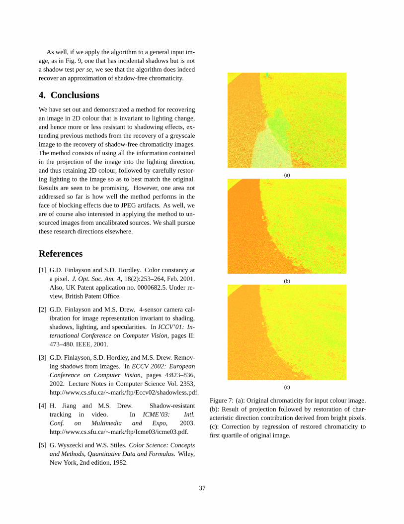
Fig. 7(b) shows the effect of restoration of an estimateof the 2-vector offset required to put the original image’s

lighting back into the recovered chromaticity. We see thatthe suggested method has indeed done quite well, comparedto the shadowed, original version Fig. 7(a).

However, the result is still not as accurate as it could pos-sibly be, and in fact we can correct this result by perform-ing a regression of the resulting chromaticityρ back to thebrightest quartile, say, in the original image. To do so, wecan transform the chromaticityρ via a3× 3 matrixM thatserves to map these pixels back to valuesρ from the inputimage. Since the result should again be a chromaticity, sothat eq. (2) is still obeyed, we should use a constrained op-timization such that the sum of each columnM i of M isunity; as well, since the range of any chromaticityρ is [0,1],elements of matrixM should also be constrained to lie inthis interval.

An optimization of this type is as follows:

min∑

(ρ orig, brightest quartile−M ρ̃ )2

with constraints

∑M i = 1, i = 1..3,

convex sum

0 ≤ M ≤ 1range of chromaticity

(16)

The result of this additional step on the image in Fig. 7(b)is shown in Fig. 7(c). While we cannot easily obtain an er-ror value for the chromaticity in this resulting image, sincewe are really concerned with both non-shadowed and shad-owed pixels and we do not have ground truth for the latter,nevertheless clearly the colour of pixels is closer to the cor-rect colour in non-shadowed pixels in the original image,especially in the colour of the footpath in the image. Therms error for the non-shadowed regions, the high-brightnesspixels, is always reduced by the algorithm by about 50% asa result of the regression step. Fig. 6 shows how the projec-tion line in Fig. 3(b) becomes a curve, after the transformback to L1 chromaticityρ given by eq. (15).

Figs. 8 and Figs. 9 show more results, using the aboveprocedure. Clearly, the method does show usefulness sincean approximation of correct chromaticity is indeed seen tobe recovered.

In Fig. 8, the input image has a large shadow area, andthis is effectively removed by the method. As well, the re-covered chromaticity quite well approximates the correctchromaticity for non-shadowed regions. For example, inFig. 8(c), the chromaticity of the sky colour is actually veryclose to that in Fig. 8(b) — this is not apparent to the eyeunless one crops the region of interest out of the image, be-cause of the simultaneous contrast effect in human vision.

36

As well, if we apply the algorithm to a general input im-age, as in Fig. 9, one that has incidental shadows but is nota shadow testper se, we see that the algorithm does indeedrecover an approximation of shadow-free chromaticity.

4. ConclusionsWe have set out and demonstrated a method for recoveringan image in 2D colour that is invariant to lighting change,and hence more or less resistant to shadowing effects, ex-tending previous methods from the recovery of a greyscaleimage to the recovery of shadow-free chromaticity images.The method consists of using all the information containedin the projection of the image into the lighting direction,and thus retaining 2D colour, followed by carefully restor-ing lighting to the image so as to best match the original.Results are seen to be promising. However, one area notaddressed so far is how well the method performs in theface of blocking effects due to JPEG artifacts. As well, weare of course also interested in applying the method to un-sourced images from uncalibrated sources. We shall pursuethese research directions elsewhere.

References

[1] G.D. Finlayson and S.D. Hordley. Color constancy ata pixel. J. Opt. Soc. Am. A, 18(2):253–264, Feb. 2001.Also, UK Patent application no. 0000682.5. Under re-view, British Patent Office.

[2] G.D. Finlayson and M.S. Drew. 4-sensor camera cal-ibration for image representation invariant to shading,shadows, lighting, and specularities. InICCV’01: In-ternational Conference on Computer Vision, pages II:473–480. IEEE, 2001.

[3] G.D. Finlayson, S.D. Hordley, and M.S. Drew. Remov-ing shadows from images. InECCV 2002: EuropeanConference on Computer Vision, pages 4:823–836,2002. Lecture Notes in Computer Science Vol. 2353,http://www.cs.sfu.ca/∼mark/ftp/Eccv02/shadowless.pdf.

[4] H. Jiang and M.S. Drew. Shadow-resistanttracking in video. In ICME’03: Intl.Conf. on Multimedia and Expo, 2003.http://www.cs.sfu.ca/∼mark/ftp/Icme03/icme03.pdf.

[5] G. Wyszecki and W.S. Stiles.Color Science: Conceptsand Methods, Quantitative Data and Formulas. Wiley,New York, 2nd edition, 1982.

(a)

(b)

(c)

Figure 7: (a): Original chromaticity for input colour image.(b): Result of projection followed by restoration of char-acteristic direction contribution derived from bright pixels.(c): Correction by regression of restored chromaticity tofirst quartile of original image.

37

(a) (b)

(c) (d)

Figure 8: (a): Input colour image. (b): Chromaticity for input colour image, including chromaticity in shadowed regions. (c):Result of projection and restoration of light, plus regression. The chromaticity of the sky region, for example, is close to thecorrect value. (d): Greyscale invariant.

38

(a) (b)

(c) (d)

Figure 9: Use of the algorithm on general input. (a): Input colour image. (b): Original chromaticity for input colour image.(c): Result of projection and restoration of light, plus regression. (d): Greyscale invariant.

39