1

Optical Memory and Neural Networks, v. 12, No. 1, 2003

Nonlinear filters for image processing in neuro-morphic parallel networks

Leonid P. Yaroslavsky

Department of Interdisciplinary Studies,

Faculty of Engineering, Tel Aviv University,

Tel Aviv 69978, Israel ABSTRACT A wide class of nonlinear filters for image processing is outlined and described in a

unified way that may serve as a base for the design of their implementations in

optoelectronic programmable parallel image processors. The filters are treated in

terms of a finite set of certain estimation and neighborhood building operations. A set

of such operations is suggested on the base of the analysis of a wide variety of

nonlinear filters described in the literature.

Key words: Image Processing, Nonlinear Filters, Optoelectronic processors 1. Introduction

Since J.W. Tukey introduced median filters in signal processing ([1]), a vast

variety of nonlinear filters and families of nonlinear filters for image processing has

been suggested. The remarkable feature of these filters is their inherent parallelism.

This motivates attempts to develop unification and structurization approaches to

nonlinear filters to facilitate filter analysis, usage and design. In this paper, a

structurization and unification approach to image processing filters based on

fundamental notions of signal sample neighborhood and estimation operations over

the neighborhood aimed at filter implementation in parallel computing networks is

2

suggested and outlined.

Throughout the paper, we will assume that images are single component signals

with scalar values. We will assume also that images are digitized i.e they are

represented as sequences of integer valued (quantized) numbers.

The exposition is arranged as following. In Sect. 2 main assumptions and

definitions are introduced. Then, in Sects. 3-5, respectively, listed and explained are:

typical pixel and neighborhood attributes, typical estimation operations involved in

the filter design and typical neighborhood building operations that were found in the

result of analysis of a large variety of nonlinear filters known from literature ([2-10]).

In Sect. 6 classification tables of the filters are provided in which filters are arranged

according to the order and the type of neighborhood they use. Iterative, cascade and

recursive implementation of filters are reviewed in Sects. 7 and 8. Sect. 9 illustrates

some new filters that naturally follow from the classification and in Sect. 10 filter

implementation in parallel neuro-morphic structures is briefly discussed.

2. Main definitions

Main assumptions that constitute the suggested unified and structurized treatment

of nonlinear filters are:

• Filtering is performed within a filter window.

• In each position k of the window, with k being a coordinate in the signal

domain, filters generate, from input signal samples kb within the window an

output value ka for this position by means of a certain estimation operation

ESTM applied to a certain subset of window samples that we will call a

neighborhood of the window central sample:

(((( ))))NBHa:ab kkk ESTM====→→→→

3

• The neighborhood is formed on the base of window sample attributes (to be

discussed in Sect.3). The process of forming neighborhood may, in general, be

multi stage one beginning from the initial W-neighborhood (Wnbh) formed from

filter window samples through a series of intermediate neighborhoods.

Intermediate neighborhoods may, in addition to its pixel attributes, have attributes

associated with the neighborhood as a whole and obtained through an estimation

operation over the neighborhood.

• Nonlinear filters can be specified in terms of neighborhood forming and

estimation operations they use

This concept is schematically illustrated in a flow diagram of Fig. 1. Filter

window samples with their attributes form a primary “window neighborhood” Wnbh.

On the next level, this first level neighborhood NBH1 is used to form, through a

number of neighborhood building operations such as shown in Fig. 1 grouping and

intermediate estimation operations, a second level neighborhood NBH2 which, in this

illustrative example, is used for generating, by means of an estimation operation, filter

output pixel for this particular position of the window. It is only natural to associate

the filter output in each position of the window with the central pixel of the window.

We will outline typical attributes of pixels and and principles of neighborhood

formation in Sect. 3 and 5, respectively.

3. Typical signal attributes

Natural primary signal sample attributes that determine filtering operations are

pixel values (magnitudes) and their co-ordinates. It turns out, however, that a number

of attributes other then only primary ones are essential for nonlinear filtering. Table 1

lists typical digital signal sample attributes that are involved in the design of nonlinear

4

filters known from the literature. As one can see from the table, these “secondary”

attributes reflect features of pixels as members of their neighborhood.

Attributes Rank and Cardinality reflect statistical properties of pixels in

neighborhoods. They are interrelated and can actually be regarded as two faces of the

same quality. While Rank is associated with variational row, i.e ordered in ascending

order sequence of neighborhood pixel values, Cardinality is associated with the

histogram over the neighborhood.

“Geometrical” attributes describe properties of images as surfaces in 3-D

spaces, respectively. Membership in neighborhood and Spatial connectedness are

binary 0/1 attributes that classify topological relationship between a given signal

sample and a neighborhood. Neighborhood elements are regarded spatially connected

if one can connect them by a line that passes through the samples that all belong to the

neighborhood.

This list of signal attributes does not pretend to be complete. Rather, it reflects

the state of the art and may suggest directions for further extensions.

4. Estimation operations

Typical estimation operations used in known nonlinear filters are listed in

Table 2. In the filter design, selection of estimation operation is, in general, governed

by requirements of statistical or other optimality of the estimate. For instance, MEAN

is an optimal MAP- (Maximal A Posteriori Probability) estimation of a location

parameter of data in the assumption that data are observations of a single value

distorted by an additive noncorrelated Gaussian random values (noise). It is also an

estimate that minimizes mean squared deviation of the estimate from the data. PROD

is an operation homomorphic to the addition involved in MEAN operation: sum of

5

logarithms of a set of values is logarithm of their product.

ROS operations may be optimal MAP estimations for other then additive

Gaussian noise models. For instance, if neighborhood elements are observations of a

constant distorted by addition to it independent random values with exponential

distribution density, MEDN is known to be optimal MAP estimation of the constant.

It is also an estimate that provides minimum to average modulus of its deviation from

the data. If additive noise samples have one-sided distribution and affect not all data,

MIN or MAX might be optimal estimations. MODE can be regarded an operation

of obtaining MAP estimation if distribution histogram is considered a posteriori

distribution of a parameter (for instance, signal gray level). RAND is a “stochastic”

estimation operation. It generates an estimate that, statistically, is equivalent to all

above “deterministic” estimates. All these estimation operations belong to a class of

“smoothing” operations SMTH since they result in data smoothing.

SPRD are operations that evaluate neighborhood data spread. Its two

modifications, “inter-quantil distance” IQDIST and “range” RNG ones, are

recommended as a replacement for standard deviation for the evaluation of spread of

data with non Gaussian statistical distribution. SIZE operation computes number of

samples that constitute the neighborhood (when it does not directly follows from the

neighborhood definition). In application to image nonlinear filtering, this operation is

less known than above ones. We will illustrate in Sect. 9 how its use can improve

efficiency of some known filters.

5. Neighborhood building operations

Neighborhood building operations can be unified in two groups: operations

that generate a scalar attribute of the neighborhood as a whole (“scalar” operations)

6

and those (vectorial) that are used in multi stage process of forming neighborhood.

The latter generate, for neighborhood elements, a new set of elements with their

attributes that form a neighborhood of the next stage. “Scalar” operations are basically

the same as those listed in Table 2. Typical vectorial operations are listed in Table 3.

One can distinguish three groups of vectorial neighborhood building

operations: functional element-wise transformations, linear combinations and

grouping/selection operations. Functional transformations are nonlinear functions

such as, for instance, logarithmic one, applied, element-wise, to all neighborhood

elements. MULT-operations assume multiplying neighborhood elements by scalar

“weight” coefficients that are selected according certain attributes (co-ordinates,

value, rank, cardinality), or combination of attributes. Replication REPL-operations

can be regarded as a version of weighting with integer weights and are used in data

sorting. A special case of replication are SELECT_A operations that select from the

neighborhood some elements (replication factor 1) and neglect others (replication

factor 0). In particular, shape-neighborhoods are formed by selection from the filter

window pixels those that form a certain special spatial shape, such as, for instance,

cross, diagonal, etc. Other examples of sub-neighborhoods formed by feature

controlled selection of neighborhood elements are shown in the table EV-, KNV-, ER-

, KNR-,Q-, CL-, FLAT-neighborhoods.

Linear combination operations multiply neighborhood elements by a matrix

and/or add/subtract a constant. Although the matrix can, in principle, be arbitrary,

orthogonal transform matrices are used in known filters.

6. Classification tables of the filters

In tables 4-7, nonlinear filters are represented grouped according to the

7

number of stages in building neighborhood they use for generating final estimation of

the filter output. The tables do not pretend to contain all filters that have been

published by now. They are mostly based on data collected in Ref.[9] as well as in

Refs. [3, 4, 8, 9, 10] to which readers can refer for detailed information regarding

properties and applications of the filters.

Table 4 lists the simplest nonlinear filters that use one-stage NBH1

neighborhood, the primary window Wnbh-neighborhood. In particular, one can find

in the table such popular in signal and image processing filters as moving average,

median and local histogram equalization filters.

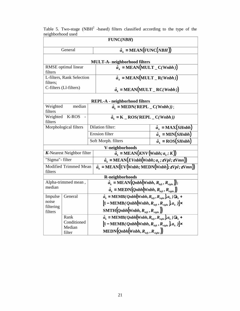
It appears that the majority of known nonlinear filters belong to the family of

two-stage NBH2 neighborhood filters listed in table 5. According to the type of the

NBH2-neighborhood used, the filters form four groups: MULT_A-, REPL_A-, V-,

and R-neighborhood filters. Some of them such as root mean square error (RMSE)

optimal linear, L- and C-filters are, in fact, families of filters.

Among three-stage neighborhood filters listed in Table 6 one can find two

large families of filters: transform domain filters and stack filters. Transform domain

filters nonlinearly modify transform coefficients of filter window samples to generate

filter output by means of applying to them operation MEAN which is an

implementation of the inverse transform for the window central sample. Two the most

advanced modifications of these filters are sliding window DCT ([8,11]) and wavelet

shrinkage filters ([12]). A popular in signal/image processing community Local

Linear Minimum Mean Square Error filter is a special case of transform domain filters

in which signal squared transform coefficients (((( )))) 2T Wnbh (signal spectral

estimations) are replaced by their mean values (((( ))))(((( ))))2STD Wnbh .

Stack filters are yet another large family of filters. They originate from the

8

idea of threshold decomposition of multilevel signals to binary signals to which

boolean functions are then applied ([13]).

Four stage neighborhood filters are exemplified in Table 7 by a family of

polynomial filters and by Weighted Majority of m Values with Minimum Range

(Shorth-) filter that implement an idea of data smoothing by averaging over data

subset that has minimal spread.

7. Iterative filtering.

An important common feature of the nonlinear filters is their local adaptivity:

the way how filter output is computed depends, in each filter window position, on

window sample attributes. In order to understand in what sense filters provide an

optimal estimate of signals one can assume that signal processing quality is evaluated

locally as well. Mathematical formulation of this assumption is provided by local

criteria of processing quality ([8]):

(((( )))) (((( )))) (((( ))))

==== ∑∑∑∑

mmmk a,aLOSSa;mLOCAVkAVLOSS

Here AVLOSS(k) is, for a signal sample with coordinate k, averaged value of losses

(((( ))))mm a,aLOSS due to replacement, by filtering, of signal “true” values {{{{ }}}}ma in

coordinates {{{{ }}}}m within the window by their estimates {{{{ }}}}ma . The averaging is two

fold. “Spatial” averaging is, in general, a weighted summation carried out over a

subset of signal samples associated with central sample k of the window (its

neighborhood NBH ). The neighborhood is defined by a locality function

(((( ))))ka;mLOC . To specify the locality function, one should, in principle, determine

“true” value ka of the central sample:

9

(((( )))) (((( )))) {{{{ }}}} (((( )))) ∈∈∈∈≠≠≠≠

====otherwise,

kNBHmif,a;mWa;mLOC k

k 00

,

where (((( ))))ka;mW are weight coefficients.

“Spatial” averaging may, in general, be supplemented with a “statistical”

averaging AV over stochastic factors involved (such as sensor’s noise, signal

statistical ensemble and alike). For such criteria, optimal processing algorithm is the

algorithm that provides minimum to averaged losses:

(((( ))))(((( )))) (((( ))))

==== ∑∑∑∑

→→→→ mmmk

abM

optk a,aLOSSa;mLOCAVminarga

where {{{{ }}}}nmbb ,==== is vector of observed signal pixels and (((( ))))abM ˆ→→→→ is a processing

algorithm.

It follows from such a formulation that optimal processing algorithm depends

on signal true values that are required to specify the locality function. For these values

are not known and are the goal of the processing, this implies that optimal estimation

algorithm should, in principle, be iterative:

(((( )))) (((( ))))(((( ))))1ESTM −−−−==== ttk NBHa

where t is iteration index. In iterative filtering, filters are supposed to converge to

“true” values. Therefore, in particular applications, filters should be selected

according to their “root” signals (fixed points).

Experimental experience shows that iterative nonlinear noise cleaning filters

substantially outperform non-iterative ones. Figs. 2 illustrates the work of some of the

filters. Some additional illustrations one can find in [13].

8. Multiple branch parallel, cascade and recursive filters

10

An important problem of iterative filtering is that of adjustment of

neighborhood building and estimation operations according to changing statistics of

data that takes place in course of iterations. This may require iterative wise change of

the filter parameters. One of the possible solutions of the problem is to combine in

one filter several filters acting in parallel branches and switch between them under

control of a certain auxiliary filter that evaluates the changing statistics.

Modification of the estimation and neighborhood building operations can also

be implemented in cascade filtering when each filter in cascade operates with its own

neighborhood and estimation operation. Note also, that, from classification point of

view, one can treat cascade filters as an implementation of hierarchical multiple stage

neighborhood filters. Several examples of cascade filters are listed in Table 8.

Computational expenses associated with iterative and cascade filtering in

conventional sequential computers can be reduced by using, as window samples in the

process of scanning signal by the filtering window, those that are already estimated in

previous positions of the window. Two examples of recursive filters are shown in

Table 9. Recursive filters are not relevant for parallel implementation.

9. Some new filters that emerge from the structurization and unification

approach

The presented approach to the nonlinear filter unification eases analysis of

structure of nonlinear filters by reducing it to the analysis of what type of

neighborhood, neighborhood building and estimation operations they use. This

analysis may also lead to new filters that “fill in” logical niches in the classification.

Several examples of such filters are given In Table 10.

“SizeEV-controlled Sigma”-filter improves image noise cleaning capability

11

of the “sigma”-filter (Table 5). Original “Sigma” filter tends to leave untouched

isolated noisy pixels (Fig. 2c). EV-neighborhood of these pixels is very small in size

since they substantially deviate from their true values. In “SizeEV-controlled

Sigma”-filter size of EV-neighborhood is computed and, if it is lower then a certain

threshold Thr, median over the window (or, in general any other of SMTH

operations) instead of MEAN(EV) is used to estimate window central pixel.

Size(Evnbh) is a useful attribute of EV-neighborhood that, by itself, can be used to

characterize image gray level local inhomogeneity (for example, as “an edge

detector”, as it is illustrated in Fig. 3, b)).

“Cardnl-filter” that generates image of local cardinality of its pixels can be

regarded as a special case of Size(Evnbh) filter for 0======== VmnVpl εεεεεεεε . It can be used

for enhancement of small gray level inhomogeneity of images that are composed of

almost uniformly painted patches (Fig. 3c)).

P-histogram equalization generalizes local histogram equalization which is its

special case for P=1. When P=0, P-histogram equalization results in automatic local

gray level normalization by local minimum and maximum. Intermediate values of P

allow flexible image local contrast enhancement. One of the immediate applications

of P-histogram equalization is image dynamic range blind calibration. EV- , KNV-

and SH-neighborhood equalizations represent yet another generalization of the local

histogram equalization algorithm when it is performed over neighborhoods other then

initial window neighborhood. One can compare conventional local histogram

equalization and EV-neighborhood equalization on Fig. 4. Some additional illustrative

examples one can find in [14].

V- and R- neighborhood based filters listed in Table 5 (K-Nearest Neighbor,

Sigma, Trimmed mean filters and alike) select from samples of the filter window

12

those that are “useful” for subsequent estimation operation by evaluation of their

“nearness” to the selected sample in terms of their gray levels and ranks. It certainly

may happen that the resulting neighborhood will contain samples that are not spatially

connected to the center of the neighborhood. One can refine such a selection by

involving an additional check-up for spatial connectivity of neighborhood elements

which is of especial importance in image filtering applications. An improved image

denoising capability of such filters was recently reported in ([17]).

10. Implementation issues

The suggested structurization of nonlinear filters for image processing implies

that a unified implementation of the filters is possible in dedicated programmed

parallel signal processors. The most natural way is to implement the filters in multi

layer parallel networks with neuro-morphic structure. Each level of such a network is

an array of elementary processors that implement estimation operations and are

connected with corresponding sub-arrays of processors on the previous layer that form

their neighborhood. The processors in each layer work in parallel and process

“neighborhood” pixels formed on the previous layer to produce output for the next

level or finally, general filter output (Fig. 5). Modern advances in “smart pixel arrays”

promise a possible electronic implementation. Another option is associated with opto-

electronic implementations that are based on the natural parallelism of optical

processors ([15]).

Figs. 6 and 7 represent illustrative examples of multi-layer networks for

computing pixel attributes and forming pixel neighborhood. The networks are

designed on the base of look-up-tables and summation units as elementary processors.

Note that the network for computing pixel rank (Fig. 6) can by itself serve as a filter

13

RANK(NBH).

11. Conclusion

It is shown that concepts of signal sample neighborhoods, estimation and

neighborhood building operations provide a unified framework for structurization and

classification of image processing nonlinear filters oriented on their implementation in

parallel multi-layer neuro-morphic networks. Many of the introduced concepts are

applicable for multi component signals such as color or multi spectral images as well,

although exhaustive extension of the approach to multi component signals requires

additional efforts.

12. Acknowledgement

The work was partly carried out at Tampere International Center for Signal

Processing, Tampere University of Technology, Tampere, Finland

14

13. References

1. J. W. Tukey, Exploratory Data Analysis, Addison Wesley, 1971

2. J. Serra, Image Analysis and Mathematical Morphology, Academic Press, 1983,

1988

3. V. Kim, L. Yaroslavsky, “Rank algorithms for picture processing”, Computer

Vision, Graphics and Image Processing, v. 35, 1986, p. 234-258

4. I. Pitas, A. N. Venetsanopoulos, Nonlinear Digital Filters. Principles and

Applications. Kluwer, 1990

5. E. R. Dougherty, An Introduction to Morphological Image Processing, SPIE

Press, 1992

6. H. Heijmans, Morphological Operators, Academic Press, 1994

7. E. R. Dougherty, J. Astola, An Introduction to Nonlinear Image Processing, SPIE

Optical Engineering Press, 1994

8. L. Yaroslavsky, M. Eden, Fundamentals of Digital Optics, Birkhauser, Boston,

1996

9. J. Astola, P. Kuosmanen, Fundamentals of Nonlinear Digital Filtrering, CRC

Press, Roca Baton, New York, 1997

10. E., Dougherty, J. Astola, Nonlinear Filters for Image Processing, Eds., IEEE

publ., 1999

11. L.P. Yaroslavsky, K.O. Egiazarian, J.T. Astola, “Transform domain image

restoration methods: review, comparison and interpretation”, Photonics West,

Conference 4304, Nonlinear Processing and Pattern Analysis, 22-23 January,

2001, Proceedings of SPIE, v. 4304.

12. D. L. Donoho, I.M. Johnstone, “Ideal Spatial Adaptation by Wavelet Shrinkage”,

Biometrica, 81(3), pp. 425-455, 1994

15

13. P. D. Wendt, E. J. Coyle, and N. C. Gallagher, Jr., “Stack Filters”, IEEE Trans.

On Acoust., Speech and Signal Processing, vol. ASSP-34, pp. 898-911, Aug.

1986.

14. http://www.eng.tau.ac.il/~yaro/RecentPublications/index.html

15. T. Szoplik, Selected Papers On Morphological Image Processing: Principles and

Optoelectronic Implementations, SPIE, Bellingham, Wa., 1996 (MS 127).

16. V. Kober, J. Alvarez-Borrego, “Rank-Order Filters With Spatially-Connected

Neighborhoods”, NCIP2001, June 3-6, 2001, Baltimore, MD, USA

16

Table 1. Typical attributes of digital signals

Primary attributes Value ak Co-ordinate k(a)

Secondary attributes Cardinality

H(a)=HIST(NBH,a)

Number of neighborhood elements with the same value as that of element a (defined for quantized signals): (((( )))) (((( ))))∑∑∑∑

∈∈∈∈−−−−====

NBHkkaaaH δδδδ

Rank

Ra=RANK(NBH,a) 1. Number of neighborhood elements with values lower than a

2. Position of value a in variational row (ordered, in ascending values order, sequence of the neighborhood elements)

3. (((( ))))∑∑∑∑====

====a

va vHR

0

COORD(NBH,R )

Co-ordinate of the element with rank R (R -th rank order statistics)

GRDNT(NBH,k ) Signal gradient in position k

Geometrical attributes

CURV(NBH,ar ) Signal curvature in position k Membership in the neighbor-hood

MEMB(NBH,a). A binary attribute that evaluates by 0 and 1 membership of element a in the neighborhood.

Spatial connectedness

CONCTD(NBH,a) A binary attribute that evaluates by 0 and 1 spatial connectedness of element a with other elements of the neighborhood

17

Table 2. Estimation operations OperationDenotation Definition

SMTH: Data smoothing operations

MEAN(NBH) Arithmetic mean of samples of the neighborhood

Arithmetic

operations PROD(NBH) Product of samples of the neighborhood

Value that occupies K-th place (has rank K) in the variational row over the neighborhood. Special cases: MIN(NBH) Minimum over the neighborhood (the first term

of the variational row) MEDN(NBH) Central element (median) of the variational row

K_ROS(NBH)

(K-th rank

order statistics)

MAX(NBH) Maximum over the neighborhood (the last term of the variational row);

MODE(NBH) Value of the neighborhood element with the highest cardinality: (((( ))))(((( ))))

aaHmaxarg

RAND(NBH) A random (pseudo-random) number taken from an ensemble with the same gray level distribution density as that of elements of the neighborhood

SPRD(NBH): Operations that evaluate spread of data within the neighborhood

STDEV(NBH) Standard deviation over the neighborhood

IQDIST(NBH) Interquantil distance (((( )))) (((( ))))NBHNBH L_ROSR_ROS −−−− , where (((( ))))NBHRL SIZE1 ≤≤≤≤<<<<≤≤≤≤ .

RNG(NBH) Range MAX(NBH)-MIN(NBH).

SIZE(NBH) Number of elements of the neighborhood

18

Table 3. Vectorial neighborhood building operations. FUNC(NBH)

Element wise functional transformation of neighborhood elements MULT_Attr(NBH)

Multiplying elements of the neighborhood by some weights MULT_C(NBH) weighting coefficients are defined by element co-

ordinates MULT_V(NBH) weight coefficients are defined by element values MULT_R(NBH) weight coefficients are defined by element ranks

MULT_H(NBH) weight coefficients are defined by the cardinality of the neighborhood elements

MULT_G(NBH) weight coefficients are defined by certain geometrical attributes of the neighborhood elements,

MULT_AA(NBH)

MULT_CR(NBH)

weight coefficients depend on combination of attributes, for instance, on both co-ordinates and ranks of neighborhood elements

REPL_Attr(NBH) Replicating elements of the neighborhood certain number of times according to

certain elements’ attribute SELECT_Attr(NBH)

Attribute controlled selection of one sub-neighborhood from a set: SELECT_A(NBH) = Subnbh

C-neighborhoods: pixel co-ordinates as attributes SHnbh Shape-neighborhoods

Selection of neighborhood elements according to their co-ordinates. In 2-D and multi-dimensional cases: neighborhoods of a certain spatial shape.

V-neighborhoods: pixel values as attributes (((( ))))Vmn;Vpl;a;NBHEVnbh k εεεεεεεε

"epsilon-V"-neighborhood A subset of elements with values {{{{ }}}}na that satisfy inequality: VplaaVmna knk εεεεεεεε ++++≤≤≤≤≤≤≤≤−−−− .

),;( KaNBHKNVnbh k "K nearest by value"-neighborhood of element ka

A subset of K elements with values {{{{ }}}}na closest to that of element ka .

RNGnbh(NBH,Vmn,Vmx)- Range-neighborhood

A subset of elements with values {Vk} within a specified range {Vmn<Vk<Vmx)

19

Table 3. Vectorial neighborhood building operations (cntd). R-neighborhoods:

pixel ranks as attributes (((( ))))Rmn;Rpl;a;NBHERnbh k εεεεεεεε

“epsilon-R”- neighborhood A subset of elements with ranks {{{{ }}}}nR that satisfy inequality:

RplRRRmnR knk εεεεεεεε ++++≤≤≤≤≤≤≤≤−−−− . ),;( KaNBHKNRnbh k -

“K-nearest by rank” neighborhood ofelement ak

A subset of K elements with ranks closestto that of element ka .

(((( ))))rightleft RRNBHQnbh ,, Quantil-neighborhood

Elements (order statistics) whose ranks {{{{ }}}}rR satisfy inequality

(((( ))))WnbhSIZERRR rightrleft <<<<<<<<<<<<<<<<1 H-neighborhoods:

pixel cardinalities as attributes (((( ))))kaNBHCLnbh ; -

"Cluster" neighborhood of element ka . Neighborhood elements that belong to the same cluster of the histogram over the neighborhood as that of element ka .

G-neighborhoods Geometrical attributes

FLAT(NBH) – “Flat”-neighborhood

Neighborhood elements with values of Laplacian (or module of gradient) lower than a certain threshold

LINEAR COMBINATION OF ELEMENTS OF NEIGHBORHOOD T(NBH) Orthogonal transform T of neighborhood elements

DEV(NBH,a) Differences between elements of the neighborhood and certain value a

SELECTION OF SUB-NEIGHBORHOOD FROM A SET OF SUB-NEIGBORHOODS

MIN_Std(SubWnbh1, SubWnbh2, …, SubWnbhn ) MIN_RNG(SubWnbh1, SubWnbh2, …, SubWnbhn )

Neighborhood standard deviation as the attribute Neighborhood range as the attribute

20

Table 4 W-neighborhood (NBH1-based) filters

Signal “smoothing” filters Moving average filter

)Wnbh(ak MEAN====

)Wnbh(_ak ROSK==== Median filter )Wnbh(ak MEDN==== MAX-filters )Wnbh(ak MAX====

"Ranked order" ("percentile") filters

MIN- filters )Wnbh(ak MIN==== Adaptive Mode Quantization filter

)WnbhMODE(ak ====

Signal “enhancement” filters Local histogram equalization

(((( ))))Wnbhak RANK====

Quasi-range filter ======== )Wnbh(ak QSRNG )WnbhL_ROS(-)WnbhR_ROS( Local variance filter

)Wnbh(ak STDEV====

21

Table 5. Two-stage (NBH2 -based) filters classified according to the type of the neighborhood used

FUNC(NBH)

General (((( ))))(((( ))))NBHak FUNCMEAN====

MULT-A- neighborhood filters RMSE optimal linear filters

(((( )))))Wnbh(_ak CMULTMEAN====

L-filters, Rank Selection filters; C-filters (Ll-filters)

(((( )))))Wnbh(_ak RMULTMEAN====

(((( )))))Wnbh(_ak RCMULTMEAN====

REPL-A - neighborhood filters Weighted median filters

))Wnbh(_(ak CREPLMEDN==== ;

Weighted K-ROS - filters

))Wnbh(_(_ak CREPLROSK====

Dilation filter: (((( ))))SHnbhak MAX==== Erosion filter (((( ))))SHnbhak MIN====

Morphological filters

Soft Morph. filters (((( ))))SHnbhak ROS==== V-neighborhoods

K-Nearest Neighbor filter (((( ))))(((( ))))K;a;WnbhKNVa kk MEAN==== "Sigma"- filter (((( ))))(((( ))))Vmn;Vpl;a;WnbhEVnbha kk εεεεεεεεMEAN==== Modified Trimmed Mean filters

(((( ))))(((( ))))(((( ))))Vmn;Vpl;Wnbh;Wnbhak εεεεεεεεMEDNEVMEAN====

R-neighborhoods Alpha-trimmed mean , median

(((( ))))(((( ))))rightleftk R,R,WnbhQnbha MEAN==== ;(((( ))))(((( ))))rightleftk R,R,WnbhQnbha MEDN====

General (((( )))) ++++⋅⋅⋅⋅==== kkrightleftk a)a,R,R,WnbhQnbh(a MEMB (((( ))))[[[[ ]]]]

(((( ))))(((( ))))rightleft

krightleft

R,R,WnbhQnbh)a,R,R,WnbhQnbh(

SMTHMEMB1 ××××−−−−

Impulse noise filtering filters

Rank Conditioned Median filter

(((( )))) ++++⋅⋅⋅⋅==== kkrightleftk a)a,R,R,WnbhQnbh(a MEMB (((( ))))[[[[ ]]]]

(((( ))))(((( ))))rightleft

krightleft

R,R,WnbhQnbh)a,R,R,WnbhQnbh(

MEDNMEMB1 ××××−−−−

22

Table 6. Three stage (NBH3-based) filters “Soft” thresholding

(((( ))));)Wnbh(ak THMEAN ⋅⋅⋅⋅====

(((( ))))[[[[ ]]]]0TTH 222 ,)Wnbh()Wnbh(maxdiag σσσσ−−−−====

Transform domain filters

“Hard” thresholding

{{{{ }}}}(((( )))))Wnbh()Wnbh(ak TTSTEPMEAN ⋅⋅⋅⋅−−−−==== σσσσ , where σσσσ is a filter parameter,

(((( ))))

>>>>≤≤≤≤

====0100

STEPx,x,

x

Local Linear Minimum Mean Square Error filter

(((( ))))(((( )))) (((( ))))(((( )))))Wnbh(

Wnbha

Wnbha kk MEAN

STDSTD1 2

2

2

2 σσσσσσσσ ++++

−−−−==== ,

where 2σσσσ is a filter parameter Double Window Modified Trimmed Mean filter

(((( ))))(((( ))))(((( ))))Vmn;Vpl;SHnbh;WnbhEVnbhak εεεεεεεεMEDNMEAN==== .

Stack filters

====ka (((( )))) (((( )))) (((( ))))(((( ))))nSubWnbh,...,SubWnbh,SubWnbh MINMINMINMAX 21

. Table 7. Four stage (NBH4-based) filters

Polynomial filters

====ka

(((( )))) (((( ))))(((( ))))(((( ))))nSubWnbh,...,SubWnbh PRODPRODMULT_CMEAN 1

Weighted Majority of m Values with Minimum Range -filters, Shorth- filters

(((( )))){{{{ }}}}(((( ))))(((( ))))(((( ))))mik SubRnbha MIN_RNGMULT_RMEAN==== ,

where (((( )))){{{{ }}}}miSubRnbh are rank based sub-neighborhoods of m

elements.

23

Table 8. Cascade filters Multistage Median Filters: cascaded median filters Median Hybrid Filters: cascaded alternating median and linear filters

Closing (((( ))))(((( ))))(((( ))))SHnbhSHbnh MAXMIN Opening (((( ))))(((( ))))(((( ))))SHnbhSHnbh MINMAX Close-opening

(((( ))))(((( ))))(((( ))))(((( ))))(((( ))))(((( ))))(((( ))))SHnbhSHnbhSHnbhSHnbh MAXMINMINMAX

Alternative sequential morphological filters

Open-closing (((( ))))(((( ))))(((( ))))(((( ))))(((( ))))(((( ))))(((( ))))SHnbhSHnbhSHnbhSHnbh MINMAXMAXMINQuasi-spread filter

======== )Wnbh(ak QSPREAD(((( ))))(((( ))))(((( )))) (((( ))))(((( ))))(((( ))))NBHWnbhL_ROS-NBHWnbhR_ROS SMTHSMTH

“Wilcoxon test”-filter

(((( ))))(((( ))))(((( ))))WnbhWnbhak RANKMEAN====

“Tamura’s test”-filter

(((( ))))(((( ))))(((( ))))(((( ))))P

k WnbhWnbha RANKMEAN==== “Median test “filter

(((( )))) (((( ))))(((( ))))(((( ))))(((( ))))2SIZERANKMEAN /WnbhWnbhsignWnbhak −−−−====

Table 9. Two examples of recursive NBH filters Recursive Median filters:

(((( ))))RecWnbhak MEDN====

Recursive Algorithm for filtering impulse noise

(((( )))) (((( )))) (((( ))))[[[[ ]]]] (((( ))))∆∆∆∆−−−−⋅⋅⋅⋅∆∆∆∆++++++++∆∆∆∆⋅⋅⋅⋅==== STEPMEANSTEP 2signRecWnbhaa kk δδδδ

where (((( ))))RecWnbhak MEAN1 −−−−−−−−====∆∆∆∆ δδδδ and 1δδδδ and 2δδδδ are detection and correction thresholds,

(((( ))))

>>>>≤≤≤≤

====0100

STEPx,x,

x

24

T able 10. Size controlled “Sigma”-filter

(((( ))))(((( ))))(((( ))))(((( ))))(((( )))) (((( ))))××××++++

××××−−−−====

SHnbhaEVnbh

ThrVmn;Vpl;a;WnbhEVnbha

k

kk

MEDNMEAN

SIZESTEP εεεεεεεε

(((( ))))(((( ))))(((( ))))Vmn;Vpl;a;WnbhEVnbhThrk

εεεεεεεεSIZESTEP −−−− , where

(((( ))))

>>>>≤≤≤≤

====0100

STEPx,x,

x .

Size_EV –filter (((( ))))(((( ))))Vmmn;Vpl;WnbhEVnbhak εεεεεεεεSIZE==== P- histogram equalization

(((( ))))(((( )))) (((( ))))(((( ))))∑∑∑∑ ∑∑∑∑==== ====

====a

v

a

v

PPk

max

vH/vHa0 0

“Cardnl-filter” )a,Wnbh(a kk HIST====

NBH2-histogram equalization EVnbh-histogram equalization

(((( ))))(((( ))))Vmn;Vpl;a;WnbhEVnbha kk εεεεεεεεRANK====

KNVnbh-histogram equalization

(((( ))))(((( ))))K;a;WnbhKNVa kk RANK====

“SHnbh-histogram equalization

(((( ))))SHnbhak RANK====

Spatially connected (SC-) EV- and R-neighborhood filters

SC-K-Nearest Neighbor filter

(((( ))))(((( ))))(((( ))))kkk a,K;a;WnbhKNVa CONCTDMEAN====

SC-"Sigma"- filter

(((( ))))(((( ))))(((( ))))kkk a,Vmn;Vpl;a;WnbhEVnbha εεεεεεεεCONCTDMEAN====

SC-Modified Trimmed Mean filters

====ka (((( ))))(((( )))) (((( ))))(((( ))))(((( ))))Wnbh,Vmn;Vpl;Wnbh;Wnbh MEDNMEDNEVCONCTDMEAN εεεεεεεε

SC-Alpha-trimmed mean, median

(((( )))) (((( ))))(((( ))))(((( ))))Wnbh,R,R,WnbhQnbha rightleftk MEDNCONCTDMEAN====;

(((( )))) (((( ))))(((( ))))(((( ))))Wnbh,R,R,WnbhQnbha rightleftk MEDNCONCTDMEDN====

25

Fig. 1 Illustrative flow diagram of signal filtering by a nonlinear filter with 2-stage neighborhood building procedure

26

a) Noisy image; noise stdev=20

b) “Sigma” filter, Evpl=Evmn=20, Wnbh=5x5

Itc) Iterative “sigma” filter, Evpl=Evmn=20,

Wnbh=5x5; 5 iterations

d) Iterative SizeEV-contr. “Sigma” filter;

Evpl=Evmn=20, Wnbh=5x5; Thr=5; 5 iterations

e) Noisy image; stdev of additive noise 20; probability of impulse noise 0.15

f) Iterative SizeEV-contr. “Sigma” filter;

Evpl=Evmn=20, Wnbh=5x5; Thr=5; 5 iterations Fig. 2 Comparison of noise suppression capability of “Sigma”- and Size-EV-controlled “Sigma”-filters

27

a) Original image

b) Size-EV-filtered image

c) Cardnl-filtered image

Fig. 3. Size-EV and Cardnl-filtering

28

Initial MRI image

RANK(Wnbh25x25)

RANK(EV(Wnbh25x25;7,7))

Fig. 4. Wnbh and EV-neighborhood local histogram equalization

29

Fig. 5. Schematic diagram of a multilayer parallel network with feedback

feedback

30

Fig. 6. Schematic diagram of a multi-layer network for computing pixel ranks

Layer of look-up-tables

Layer of look-up-tables

Layer of summation units

Layer of summation units

Input layer Output layer

31

Fig. 7. Schematic diagram of a network for forming EV-neighborhood of a pixel with gray level v .

IOutput Layer of look-up-tablesInput layer