recovery, treatment, and recycling a thesis the
TRANSCRIPT

RECOVERY, TREATMENT, AND RECYCLING
OF INDUSTRIAL WASTEWATER
by
KRISTIE LEA WITTER, B.S.
A THESIS
IN
CIVIL ENGINEERING
Submitted to the Graduate Faculty of Texas Tech University in
Partial Fulfillment of the Requirements for
the Degree of
MASTER OF SCIENCE
IN
CIVIL ENGINEERING
Approved
Accep;ted
December, 1997

Ac g06 ^^''''' 13 I o^q 7 ACKNOWLEDGMENTS
C^lp' ^ I am indebted greatly to the members of my committee for their support and
direction of this thesis and for their most valuable criticism and academic nourishment.
Dr. Raghu Narayan, Dr. John Borrelli, and Dr. Ralph H. Ramsey III. A special thanks
to Dr. Richard Tock for his aid in the final examination of this research. For their
academic expertise, advice and direction, I wish to express my appreciation to
Dr. Tony Mollhagen and Dr. Alex Gilman.
A special thanks is extended to all the employees at Texas Instruments in
Lubbock, Texas, for without whose help this project could not have been completed.
I particularly wish to acknowledge Fernando Alvarez-Lara, Galen Kunka, Yimin
Chiou, Cindy RufiF, and Gerald Hector for their support above and beyond what was
requested. In addition, I wish include Ms. Shannon Reed in my acknowledgments for
the inner strength and fiiendship that she gave me during some of the most difficult
and best of times. It has made all the difference in my life!
Finally, I wish to thank each of my fiiends and family members for their
patience, understanding, and support throughout the entire course of this project. My
feelings are best stated by I Corinthians 12:26, "and if one member suffers, all
members suffer with it; or if one member is honored, all the members rejoice with it."
This has been particularly true throughout the course of my academic studies. For
their support during the trying times, I wish to honor and rejoice with them now.
Finally, I wish to give thanks to God, for it is through Him that all things are possible!
ii

TABLE OF CONTENTS
ACKNOWLEDGMENTS ii
LIST OF TABLES v
LIST OF FIGURES vii
CHAPTER I. ESTTRODUCTION 1
1.1 Purpose 2 1.2 Objectives 5 1.3 Case Study (Overview) 5
II. REVTEW OF LITERATURE 7 2.1 Treatment Options 7 2.2 Precipitation 8
2.2.1 Lime 10 2.2.2 Activated Alumina 13
2.3 Electrocoagulation 18 2.4 Reverse Osmosis 21 2.5 Additional Treatment Options 26
2.5.1 Evaporation 26 2.5.2 Demineralization 27 2.5.3 Filtration 27
2.6 Disposal of Concentrated Wastewater 28 2.7 Examples of Water Management Programs 29
2.7.1 Case Study One 30 2.7.2 Case Study Two 30
IIL METHODOLOGY 32 3.1 Identify The Problem 33 3.2 Analyze and Solve the Problem 33
3.2.1 Water Inventory 34 3.2.2 Sample Collection 34 3.2.3 Inventory of Contaminants in Each Stream 36
3.3 Presentation of Alternative Solution(s) 37 3.3.1 Statistical Analysis 37 3.3.2 Treatment Options 39 3.3.3 Economic Evaluation 40 3.3.4 Overview 41
ni

rv. SITE SPECIFIC CASE STUDY 43 4.1 Identification of Case Study Problem 43
4.1.1 Experimental Procedures 44 4.1.2 Level of Technology 44 4.1.3 Experimental Parameters 45
4.2 Analysis of Case Study Problem 46 4.2.1 Water Inventory 46 4.2.2 Sample Collection 47 4.2.3 Inventory of Wastewater Contaminants 52
4.2.3.1 Salt Analysis 52 4.2.3.2 Metal Analysis 53 4.2.3.3 Additional Analysis 53
4.3 Presentation of Solution 62 4.3.1 Statistical Analysis 62
4.3.1.1 Accepting Sample Collection Sets 62 4.3.1.2 Determining Quality of Sample Set 65 4.3.1.3 Comparative Analysis of
Wastewater to Tap Water 70 4.3.2 Treatment Options 75 4.3.3 Economic Evaluation 75
4.3.3.1 Present-Worth Method 76 4.3.3.2 Cost/Benefit Ratio 78
4.4 Case Study Summary 79 4.5 Case Study Recommendations 80
V CONCLUSIONS AND RECOMMENDATIONS 81 5.1 Conclusions 81 5.2 Recommendations 82
LIST OF REFERENCES 83
APPENDIX 87
i\

LIST OF TABLES
2.1 Fluoride Removal by Lime Precipitation 12
2.2 Concentration of Fluoride Ion Absorbed
per Unit Weight of Activated Alumina 16
2.3 Electrocoagulation Removal Efficiencies 20
2.4 Water Quality Statistics for Case Studies One and Two 31
2.5 Savings Each Year From WMPs at Case Study One and Two 31
4.1 Approximate Water Inventory 46
4.2 Acid Wastewater Analysis 50
4.3 Salts Analysis for Data Set A 54
4.4 Salts Analysis for Data Set B 55
4.5 Salts Analysis for Data Set C 56
4.6 Metal Analysis for Data Set A 57
4.7 Metal Analysis for Data Set B 58
4.8 Metal Analysis for Data Set C 59
4.9 Conductance, pH, and TS for Data Set B 60
4.10 Conductance, pH, and TS for Data Set C 61
4.11 Reliability Levels of Data Sets A, B, and C 64
4.12 Conventional Quality Control Data for Sample Set C 65
4.13 Limits on Comparative Analysis of Industrial Wastewater to Tap Water 70
4.14 Central Tendencies and Standard Deviations of Data Set A 72

4.15 Central Tendencies and Standard Deviations of City Tap Water 72
4.16 Pearson Product Moment Correlation Coefficients 73
4.17ConfidenceRangefor99, 95, 90, and 85 Percent 74
4.18 Summary of Present Worth for Various Interest Rates 77
4.19 Summary of Cost/Benefit Ratios at Various Interest Rates 79
w

CHAPTER I
ESriRODUCTION
What community or industry is not dependent upon a reliable, cost-effective
source of potable water? Whether it is for brewing your Sunday morning coffee, as
rinsewater in a manufacturing plant, food processing facilities, or the need is 18+
megaohm-cm, ultra pure quality for rinsing micro chips in the semiconductor industry,
water is necessary for domestic, commercial, and industrial uses. Its use for non-
domestic purposes include washing, cooling, rinsing, and diluting. In recent years,
increasing concern has been expressed over the depletion of natural resources, of fi'esh
water resources - the commodity of interest in this research.
Water is a resource that is essential in many manufacturing industries. For the
semiconductor industry, water is often purchased fi'om a local municipality, sent
through a series of operations, and then discharged to Publicly Owned Treatment
Works (POTWs) with many constituents at a cleaner concentration level then the
originally purchased supply and a few constituents at much higher quality levels. The
same unit of water is essentially paid for twice (purchase and discharge costs) by each
industrial plant that requires its use. Therefore, a double economic incentive is
presented to recycle this water: reduction of water purchase cost and reduction of
water disposal cost. These incentives are in addition to the numerous intangible
benefits of conserving a natural resource and can be accomplished by establishing a

water management program (WMP). However, it is the economic considerations that
most often drive decisions in the industrial world, and not the intangible.
What is a water management program? It is a plan whose goal is conservation
of water resources in order to minimize cost and resources. Regional annual climate
conditions, local water demand, impact of an industry on a local community (tangible
and intangible), a labor pool to meet operation and maintenance needs, water/mineral
rights, and plans for a fiiture of increased use rates with decreasing resources are all
justifications for implementing a water management program. However, it is either
regulations or economics that drive industries to implement a WMP. Water is utilized
as a raw material for most industries and, therefore, a cost of production. A
dependable raw material supply is necessary to prevent a slowdown or possibly even a
complete shutdown of plant operations. Water management programs are designed to
prevent a plant slowdown or shutdown fi-om occurring which could lead to a loss of
revenue. Therefore, the goal of this research is determining the feasibility of a water
management program for semiconductor/wafer fab manufacturing plants.
1.1 Purpose
This research has been conducted to design and propose general procedures
for a water management plan for semiconductor/wafer fab wastewater. The specific
water management goal is conservation of industrial water by treating some or all of
the wastewater for reuse and recycling within the plant. The recycling process is
essentially the conversion of industrial wastewater to dionized water (DI). Ultimateh,
2
this will conserve both financial and natural resources. Determining the most cost-
effective treatment technology to apply in each series of processes will be a major step
in the general procedures. This is important because if a process is not economical,
then it will not be readily pursued by industries, unless dictated by regulations or laws.
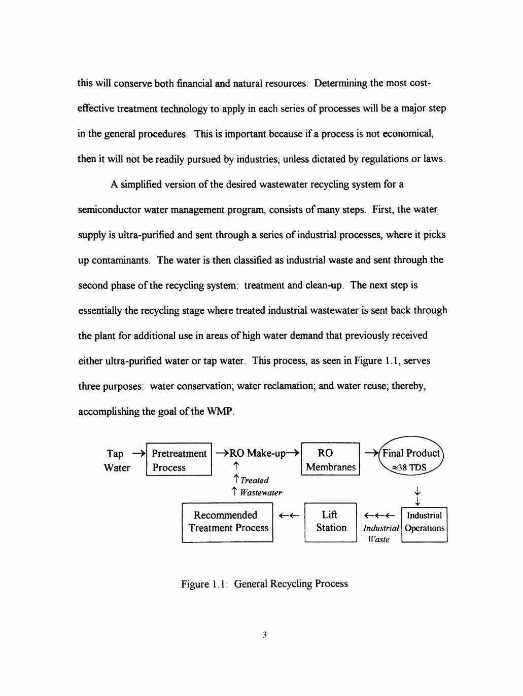
A simplified version of the desired wastewater recycling system for a
semiconductor water management program, consists of many steps. First, the water
supply is ultra-purified and sent through a series of industrial processes, where it picks
up contaminants. The water is then classified as industrial waste and sent through the
second phase of the recycling system: treatment and clean-up. The next step is
essentially the recycling stage where treated industrial wastewater is sent back through
the plant for additional use in areas of high water demand that previously received
either ultra-purified water or tap water. This process, as seen in Figure 1.1, serves
three purposes: water conservation; water reclamation; and water reuse; thereby,
accomplishing the goal of the WMP.
Tap - > Water
Pretreatment Process
—^RO Make-up-^ t 1 Treated \ Wastewater
Recommended Treatment Process
RO Membranes
Final Product J5i38 TDS
i
Industrial Waste
Industrial Operations
Figure 1.1: General Recycling Process

Management in the semiconductor industry are realizing the importance of
total water management, particularly in arid regions where water is a limited resource
The main concern of treating the industrial wastewater and recycling it back through
the plant is the quality of the recycled water and the economic feasibility of
implementing a new program to an existing program. Many semiconductor plants
constructed in the past five years have included a water management program as part
of their design and management plans. Recent changes in manufacturing technologies
have contributed to innovations that allow for lower acid strength requirements which
result in lower concentrations of residuals in the wastewater stream. This reduces the
contaminant strength in the final wastewater stream (Williams, 1997).
Older fab plants that do not have the latest technological upgrades are required
to continue to use the same high concentration acids as they did when they were
originally constructed. A plant built in 1970 compared to a plant built in 1990 has the
technological ability to produce the same end product, but the resuh is a higher
concentration of acid in the wastewater stream. Therefore, the focus of this research
is to develope a general procedure for the semiconductor industry to design WMPs
that currently do not have a water recycling program. A case study was conducted,
that followed the general procedures of the WMP presented in this research. Since no
two plants operate under the same conditions, the general procedure is flexibly
structured to allow for modifications. A WMP should be designed to meet the
individual needs at each site where it is to be implemented.
1.2 Objectives
Determining the feasibility of recycling industrial wastewater at a water quality
level acceptable for multiple industrial operations requiring high water demands was
met through four objectives. Those four objectives were:
1. To perform a water inventory/balance of high water demand processes that either
contribute to the final industrial or acid waste stream, or would be considered a
candidate for use of recycled water,
2. To segregate and sample industrial and acid waste lines for the purpose of
identifying specific pollutants present in each wastewater stream (based on
chemical characteristics),
3. To examine treatment possibilities for removing contaminants fi-om the wastewater
streams to a water quality level equal to or better than that of the current water
supply, and
4. To determine the economic feasibility of implementing a WMP.
1.3 Case Study (Overview)
A semiconductor facility built in the 1970s is currently purchasing up to
300-gpm of potable water and then discharging approximately 300 gpm of wastewater
each day. In a facility that operates 24-hours a day and seven days a week, the total
discharge volume is potentially between 216,000 gallons and 432,000 gallons each
day. That means that a possible 152 million gallons of wastewater is discharged each
year. At a cost of approximately $2.60 per 1000 gallons, an economic incentive is
5

definitely enough motivation for implimenting a water management program (Alvarez,
1997).
The 152 million gallons of wastewater produced by the different plant
operations, originated fi'om tap water. That tap water was sent through a series of
pretreatment processes including a reverse osmosis system to obtain DI quality and
then sent through the facility where in some areas it was contaminated with high
strength acids such as hydrofluoric (HE), phosphoric (PO4), and sulfiiric (SO4).
The wastewater streams are segregated into an acid waste stream and an
industrial wastewater stream. However, a portion of the acid waste enters the
industrial wastewater stream. The industrial wastewater stream is the proposed
feedwater source for the recycling program based on its quality and quantity, as
presented in this research. The results and conclusions of this case study are based on
results of the statistical analyses and economic evaluation.

CHAPTER n
REVIEW OF LITERATURE
The literature search for wastewater treatment processes possible for a WMP
included those that could be put in a single or multi-stage treatment system for
industrial wastewater fi-om semiconductor manufacturing plants. The processes for
the first stage of treatment included: absorption, precipitation, electrocoagulation, and
evaporation. After selection of one or more than one of these processes linked in
series, the recycling stream then enters the uhra-purification stage of treatment for
additional cleaning: membrane separation by reverse osmosis. The purpose of having
a muhi-stage system is the high quality requirements for the semiconductor industry.
Initially, all possibilities were considered regardless of economic feasibility.
Once the options were evaluated on technical efficiency, they were assessed on
economic merit. Then, the treatment options were narrowed down to three processes.
2.1 Treatment Options
Because of its high concentration in semiconductor wastewater and difficulty in
the removal/treatment process, one of the elements singled out for the treatment
process was fluoride. Fluoride comes fi-om hydrofluoric acid, a primary component in
chemical etching in the semiconductor industry (Varuntanya, 1994). Because of this
process, the concentration of the fluoride in semiconductor wastewater is high, greater
than 20 mg/L. This is particularly common for older facilities that must use stronger
concentrations of acids (5 percent or more) for the etching process. Newer facilities
have the technological ability to use lower strength acids (0.5 to 1 percent), that
resuhs in lower contaminant levels in the wastewater (Williams, 1997). Many
treatment options for wastewater with high concentrations of fluoride do not remove
enough of the dissolved fluoride complexes to meet water quality requirements
suitable to send the effluent back through the DI plant or through a reverse osmosis
system (Stuart, 1937; Clifford, 1986; Lindsey, 1993). The following processes were
considered as possibilities for treating semiconductor wastewater:
-low temperature evaporation -activated alumina
-absorption (ion exchange) -precipitation
-activated carbon -electrocoagulation
-lime softening -contact filters.
Precipitation by lime or hydrated lime, absorption/precipitation by activated
alumina, and electrocoagulation were the primary focus of the literature search, since
each has the capacity to effectively remove high concentrations of fluoride (CWC,
1994; US Fiher, 1997; ECS 1997). The other treatment options are noted at the end
of this chapter, but were not proven to be as efficient or economical as the three
processes first mentioned (Stuart, 1937; Clifford, 1986; Lindsey, 1993).
2.2 Precipitation
Precipitation is the chemical process by which specific dissolved solids are
transformed into insoluble particles, causing them to fall out of solution. Specifically,
8

Ca ', Mg " , Fe ', Fe^\ COs ', and HPO/' are polyvalent cations and anions that are
readily removed fi'om solution by precipitation. More common to semiconductor
wastewater, F", Si(0H)30", and H2As04', can be removed by coprecipitation or
absorption by hydrated lime (Clifford, 1986).
Precipitation is a good treatment option for the removal of a select one or two
contaminants. However, it is generally not effective for removing all contaminants
from a wastewater stream (Montgomery, 1985). The efficiency of the precipitation
process is dependent upon pH, alkalinity, competing ions, and chelant concentration
(Clifford, 1986).
Precipitation techniques are generally preferred for lower concentrations of
fluoride (10 to 20 ppm) in wastewater, but have the disadvantage of sometimes
producing a residual sludge for disposal (Maier, 1947). In addition, precipitation
processes do not readily respond to large fluctuations in influent concentration and
require a stoichiometric feed of reagent material (Montgomery, 1985). Advantages of
precipitation processes are;
1. low cost and reliability,
2. effective over a wide range of temperatures, and
3. selective for fluoride.
Disadvantages include:
1. requirement for stoichiometric additions of reagent,
2. sludge disposal,
3. varying coprecipitation dependability, and
9

4. optimal pH is usually high (Maier, 1947; Montgomery, 1985; Clifford, 1986;
Lindsey, 1993).
Two precipitation processes were considered for removing the specific
contaminants in semiconductor wastewater. Those processes were
1. precipitation by addition of lime, and
2. precipitation by the addition of activated alumina, which is considered a
combination absorption and precipitation reaction (Lai, 1996).
2.2.1 Lime Precipitation
Precipitation with lime is a common practice for the removal of fluoride, called
fluoridation and is referred to as water softening (Varuntanya, 1996). Precipitation of
fluorides using lime is dependent upon the existing magnesium and hydrogen ion
concentrations, but is a good candidate for semiconductor wastewater because it
specifically removes fluoride from liquid solutions (Stuart, 1937). However,
precipitation with lime alone does not remove enough of the fluoride present in the
wastewater to reach the desired final concentration required for recycling (US Filter,
1997). Therefore, variations with other chemicals and lime are required.
One effective precipitation combination is chloride and lime (US Filter, 1997).
Calcium chloride and calcium hydroxide remove fluoride at an optimal pH range of 6-
to-9. The sludge byproduct from this process was approximately 18 percent of the
original volume, but could be reduced to 8 percent with the addition of alum
10

(Varuntanya, 1994). In this process, CaCOs precipitates out when lime reacts with the
bicarbonate in the solution. As with most precipitation reactions, this requires
stoichiometric dosages. Through coprecipitation with magnesium hydroxide, fluoride
can be removed in the form of an insoluble particle (Varuntanya, 1996).
The following equation is a calculation of the amount of magnesium (mg/L)
required to remove desired levels of fluoride from wastewater (Montgomery, 1985).
Fresidual = Finitial - ( 0 . 0 7 * FinitiaWMg )
Equation (2-1) Where: Fre8iduai= desired level of fluoride in the effluent
Finitiai= initial fluoride concentration in the influent Mg = magnesium concentration required for treatment 0.7 = equation constant
Lime precipitation is not uncommon and there have been many pilot studies
conducted on the process. In a case study on fluoride removal from water provided by
US Filter Corporation, wastewater containing 300 ppm fluoride at a flow rate of 7.3
gpm was treated to < 5 ppm using hydrated lime (Memtec, 1997). Aluminum chloride
and calcium chloride were added to the wastewater in an acidic range. Calcium
hydroxide was then added to raise pH levels to an average of 7.5 to 8.0. In this
process, the fluoride goes through two chemical reactions, then becomes insoluble,
and finally is removed through filtration (Memtec, 1997).
Lime was combined with various other chemicals to examine the removal
efficiencies of different dosages with different precipitation chemicals. This was done
because lime can not remove sufficient levels of fluoride when used alone. A
11

combination of aluminum/calcium and chloride/lime produced the best resuhs for
removing fluoride, as seen on Table 2.1.
Table 2.1: Fluoride Removal by Lime Precipitation Test
Numl)er
1
2
3
4
Efficiency of Fluoride Removal by Lime Precipitation
Fluoride (ppm)
CaCl2/H3P04/Llme Chemistry
pH adjusted to 6.0-7.0 with NaOH Added 1600 ppm CaCb Added 1400 ppm H3PO4
pH adjusted to 8.0-9.0 with lime Filtered (2.5 um)
Initial 390
43
Alumlnum/CaCb/Lime Chemistry
pH adjusted to 3.0-4.0 with NaOH Added 1100 ppm CaCb
Added 500 ppm A! as AlCIa pH adjusted to 7.0-8.0 with lime
Filtered (2.5 um)
Added CaCb at ratio Ca:F, 1:1 at initial pH (pH = 2.60)
Added AICI3 at ratio AI:F, 1:1 pH adjusted to 7.5-8.0 with lime
Filtered (2.5 um)
Initial 470
9
Initial 290
3
Alumlnum/CaCl2 Chemistry
Added CaCb at ratio Ca:F, 1:1 at pH=2.6 Added AICI3 at ratio AI:F, 1:1
pH adjusted to 7.5-8.0 with NaOH Filtered (2.5 um)
Added CaCb at ratio Ca:F, 3:1 at pH=2.6 Added AICI3 at ratio AI:F, 3:1
pH adjusted to 7.5-8.0 with lime Filtered (2.5 um)
Initial 290
27
Initial 290
8
Aluminum/Lime Chemistry
Added AICI3 at ratio AI:F, 2:1 at pH=2.6 pH adjusted to 7.5-8.0 with lime
Filtered (2.5 um)
Target Concentration
Initial 290
5
5 Source US Filter Co., 1997
12
2.2.2 Activated Alumina
As early as 1934, studies on absorption processes made by McKee and
Johnston indicated that the removal efficiency rate of fluorides increases with a
decrease in pH (McKee, 1934). This is beneficial for semiconductor wastewater as the
majority of wastewater from the chemical etching process has a pH < 5.
The second treatment process is a combined precipitation and absorption
process through activated alumina (aluminum oxide). Studies have been conducted by
the National Environmental Engineering Research Institute (NEERI) since the 1960s
on this process with defluoridation of water by activated alumina (Bulusu, 1990).
Activated alumina utilizes the hydrolytic absorption properties of the alumina (an
amphoteric compound) to remove the fluorides from solution (Quasim, 1998).
Activated alumina is largely pH dependent (best below pH 8.2) because the pH of the
solution effects the solubility of the inorganic fluoride (HF) in the water (Sorg, 1978).
The absorption capacity of fluoride to activated alumina decreases as the solution
becomes alkaline and appears to be at an optimal absorption level in the range from pH
4.0 to 5.5 (Lai, 1996).
Activated alumina is sometimes referred to as an absorption process, ligand
exchange, or sometimes even as chemisorption because the contaminant ions (such as
fluoride ions) are exchanged for hydroxides on the alumina surface (Clifford, 1986).
These reactions are highly specific and endothermic (Lai, 1996). In an acid solution,
fluoride goes through the following surface exchange reactions. The following
13

chemical reaction shows the removal of fluoride from a water solution (Clifford,
1986).
=Al-OH- + ir+F<->
= Al - F + HOH Equation (2-2)
There is an equal exchange (one-to-one molar ratio) of a hydroxyl group
(OH") for a fluoride ion (F"). Fluoride, the most electronegative of all the elements,
bonds to the hydroxyl site with the activated aluminum (Dillon, 1992). The fluoride
absorption to the aluminum takes place when the wastewater is passed through
columns containing beds of activated alumina (Savinelli, 1958). Figure 2.1 shows a
bench scale set-up for fluoride removal through activated alumina.
n 55-gal Drum
4-liter Erienmeyer
Flask
nu
Manifold (12 outlets)
^ i Water Level
Column
Rotameter
T T
Water Level Control
r 1 n_"
• • • • • • *
Alumina Bed
Perforated Clay Disc
U-Overflow
Overflow Tank w2\
Overflow Pump 5
Figure 2.1. Activated Alumina Bench Scale Set-Up Source: SavineUi, 1958
14
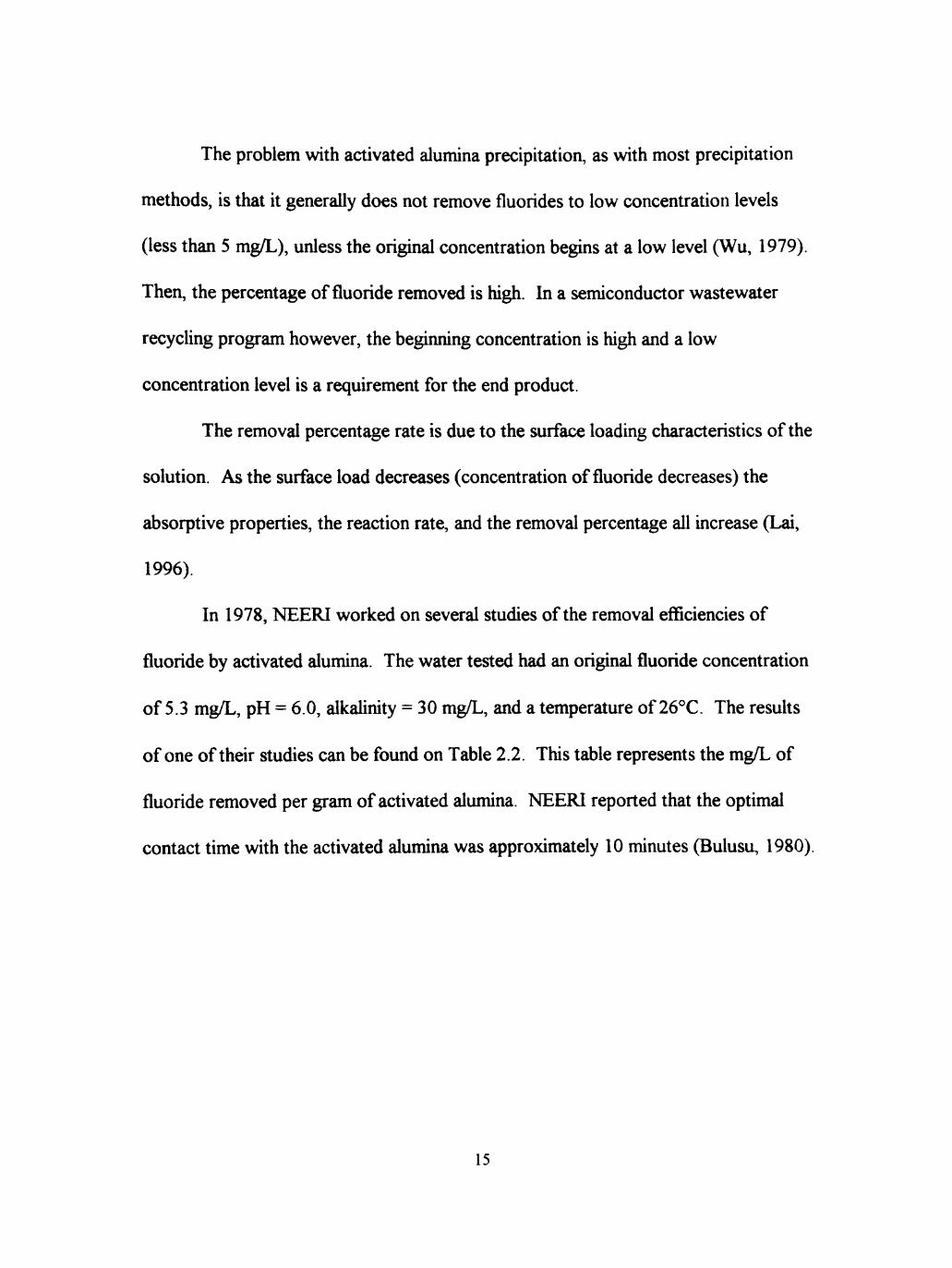
The problem with activated alumina precipitation, as with most precipitation
methods, is that it generally does not remove fluorides to low concentration levels
(less than 5 mg/L), unless the original concentration begins at a low level (Wu, 1979).
Then, the percentage of fluoride removed is high. In a semiconductor wastewater
recycUng program however, the beginning concentration is high and a low
concentration level is a requirement for the end product.
The removal percentage rate is due to the surface loading characteristics of the
solution. As the surface load decreases (concentration of fluoride decreases) the
absorptive properties, the reaction rate, and the removal percentage all increase (Lai,
1996).
In 1978, NEERI worked on several studies of the removal efficiencies of
fluoride by activated alumina. The water tested had an original fluoride concentration
of 5.3 mg/L, pH = 6.0, alkalinity = 30 mg/L, and a temperature of 26°C. The resuhs
of one of their studies can be found on Table 2.2. This table represents the mg/L of
fluoride removed per gram of activated alumina. NEERI reported that the optimal
contact time with the activated alumina was approximately 10 minutes (Bulusu, 1980).
15

Table 2.2; Concentration of Fluoride Ion Absorbed per Unit Weight of Activated Alumina
Time
(minutes)
1
5
10
30
60
120
180
Weight of Activated Alumina (grams)
0.5481
1 64
1.62
2.01
2.1
2.1
2.19
2.37
1.0652
1.37
1.52
1.61
1.66
1.8
1.85
1.94
2.0866
1 15
1,2
1.25
1.32
1.39
1.41
1.44
3.1454
1.08
1.13
1.15
1.15
1.19
1.21
1.24
4.0212
0.9
0.95
0.97
0.98
0.99
0.99
1.01
5.1257
0.72
0.75
0.77
0.78
0.8
0.82
0.83
7.1237
0.55
0.57
0.59
0.6
0.62
0.63
0.64
10 212
045
0.47
0.48
0.48
0.48
0.49
0.49
Source: Bulusu, 1980
Although activated alumina has effective removal rates at low concentrations,
its regeneration rate is costly. That is because it is regenerated through the use of both
an acid and a base or by thermal regeneration at around 800°F that leads to increased
energy requirements (Onuoha, 1983). Regeneration is necessary once the alumina
resin is exhausted by fluoride absorption (Onuoha, 1983). Both regeneration forms
are costly, which leads to an overall costly treatment process when compared with
alternative treatment processes such as hme precipitation (Montgomery, 1985). In
1947 when most of the activated alumina studies were conducted, the cost of chemical
regeneration was $275 per milligram of alumina (Maier, 1947). The reaction below
shows the regeneration of activated alumina after fluoride removal (CUffi rd, 1986).
Al-F + OH- = = Al - OH + F' Equation (2-3)
This is the reverse reaction of Equation 2-2 where chemical addhion was made
with a strong hydroxyl group such as NaOH or Ca(0H)2 (Mann, 1997). The fluorine
is released fi-om the activated alumina by absorption to sodium or calcium to form an
16
insoluble salt: NaF or CaF (Dillon, 1992). The regenerative energy requirement for
this process makes it an uneconomical approach for processing industrial wastewater
as seen in the economic evaluation of the provided case study (Chapter IV).
The two precipitation methods of hydrated lime and activated alumina, as with
most precipitation methods, involves the stoichiometric addition of chemicals to the
wastewater stream for the purpose of removing a target element or elements. Any
time a chemical additive is required for a treatment process, the chemical will always
be required to continue use of the process; that would be costly if your chemical cost
is high or your regenerative process requires costly chemicals (as with activated
alumina). Advantages of using activated alumina include:
1. operates on demand for changes in concentration and flow (until the resin has met
its maximum exchange capacity),
2. has an optimal pH range of 5.5 to 8.5, and
3. is highly selective for fluoride ions.
Disadvantages include:
1. the requirement of either an acid and a base or high thermal levels to regenerate
the activated medium, and
2. the media breaks down and must be both disposed of and replaced (Maier,
1947; Onuoha, 1983; Montgomery, 1985; Cliffi)rd, 1986).
17

2.3 Electrocoagulation
The next treatment option is electrocoagulation (EC). Electrocoagulation is
the addition of an electrical current (either AC or DC) through a fluid via conductive
plates (alloy, aluminum, or iron) to destabilize and coagulate target elements or
complexes (Kaselco, 1997). This is a unit operation for the purpose of removing
anions and cations fi-om the solution. The resuU is a demineralized, neutrally charged
water (Zentox, 1997). The ions and other charged particles become neutralized and
precipitate out of suspension or solution (Zentox, 1997). This creates larger, heavier
particles in a matter of seconds that can then be removed from the wastewater stream
by a separation process, such as filtration, settling basins, centrifugal separation, or
clarification (Zentox, 1997). The removal rate is dependent on the time and volume
operating constraints (Zentox, 1997). A flow diagram, of the EC process can be found
on Figure 2.2.
This process has a high efficiency and is not subject to fouling by most
dissolved solids or suspended solids including bacteria, heavy metals, radionuclides,
fats/oils/grease (FOGs), or other ions. Responsibility of disposing the recovered metal
products can be eliminated by resmehin-g the oxidized form, of the metals recovered in
the byproduct (Global Wind, 1997), There are no hazardous by-products to this
process because all particles that are removed from the water are neutralized,
inactivated molecules (Armstrong, 1997). On Table 2.3, a list of the removal
efficiencies by EC from various industrial operations (chemical, battery manufacturers,
plating, boilers, mining, crude oil, etc.) can be found (ECS, 1997).
18

Influent
i
Dual Low-Pressure
Filters (if influent ->50 micron)
Sludge Disposal
Sludge Unit
t
Chemical Adjustment and Additives
Electrocoagulation Unit
Additional Treatment
Dual Low-Pressure
• Filters (if influent >10 micron)
00 t
t
Figure 2.2; General Flow Diagram of the Electrocoagulation Process
In addition to the previously mentioned advantages, this process can handle
high flow rates and still maintain an efficient removal rate (Zentox, 1997). If a process
shutdown is required, the wastewater is sent to a surge tank. Although the capital cost
is high for this type of treatment system («$275,000 for a 300 gpm system, but is
dependent upon the size of the system), it pays for itself quickly (Armstrong, 1997).
Operational costs are reduced by eliminating discharge fees, fines, and reducing the
purchased water volume. The system requires one operator to oversee the process via
19

a computer that monitors the wastewater as it passes through the system (Armstrong,
1997). In addhion, the process has the capacity to add revenue by harvesting
resources fi-om the by-products that precipitate out of solution (dependent upon the
waste constituents) (Global Water, 1997).
Table 2.3: Electrocoagulation Removal Efficiencies
Contaminant
Removed
Arsenic
Barium
Caiciunn
Cadmium
Chrome
Copper
Gold
Iron
Lead
Magnesium
Manganese
Nickel
Selenium
Silicon
Silver
Source of
Water
Chemical Mft.
Battery Mft.
Boiler
Plating
Manufacturing
Battery
Plating
Well
Battery Mft.
Mine
Manufacturing
Plating
Mine
Manufacturing
Mining
(PPM) Before Treatment 900
30
1230
46
900
25
6
106
90
65
3
43
1
53
5
(PPM) After Treatment 0.125
<0.050
6
<0.003
<0.003
N/D
N/D
<0.005
<0.003
2
0.3
0.06
N/D
0.03
N/D
Contaminant
Renwved
Sulfur
Tin
Zinc
Chlorinated
Hydrocartxms
i 1 1 i 1
1 1 1
Source of
Water
Crude Oil
Plating
Plating
Landfill Leachate
Cyanide, Total
Oily Cooling Waters
Food Oils and Water
Animal Fats
Rendering
Cooking Fats
Nitrates
Fabric Dyes
Paracresol Methyl
Methyl Dihal
BOD'S Tanker wash
(PPM) Before Treatment 5,000
50
80
340
62
1500
26000
5700
4200
18000
500
180000
1000
2200
96000
(PPM) After
Treatment
0.08
0.006
0.008
13
0.06
38
4
90
54
86
54
4
41
36
150
Costs for water purchases and discharges can be reduced (on an average) from
$2.60 per 1000 gallons of water to approximately $0.40-0.50 per 1000 gallons of
water (Armstrong, 1997). This cost includes the power cost, cell costs, and cost for
any chemical additives. With these savings, the capital cost can often be recovered in
12 to 18 months of initial system start-up (Global Water Ind., 1997). In addition, the
system allows for closed loop wastewater recycUng which is an added benefit to the
water management program (Global Water, 1997).
20

Advantages to using an EC system include:
1. only 3 to 5 percent loss of total wastewater volume during treatment process to
brine and evaporation,
2. replacement of electrode cells is quick and easy (approximately 30 minutes), and
3. operates at high efficiency rates.
Disadvantages include:
1. high capital cost, and
2. lack of long term data on process operations; no more than 10 years worth of data
available at this time (Global Water Industry 1947, Armstrong 1997, Zentox 1997, and
Kaselco, 1997).
2.4 Reverse Osmosis
Regardless of which first stage treatment process is chosen, an ultrapure
water will be required for a semiconductor facility (Kemp, 1997). Therefore, a reverse
osmosis (RO) system is suggested for use to obtain the required quahty level. This is
an obvious choice (as shown on Figure 2.3.) for treating industrial wastewater because
RO systems have the capacity to efficiently remove large portions of TDS and quickly
produce large quantities of ultrapure water (Aurich, 1995).
21
Feedwater Supply
•Wastewater •Analysis
Pretreatment
•Scale Control •Metal Oxides
High Pressure Pumps
•Pressure •Flow Rate
RO Membranes •Salt Rejection •Resistance
Post Treatment
•Degasification •pH adjustment
End Use
•Ultra Pure •Industrial
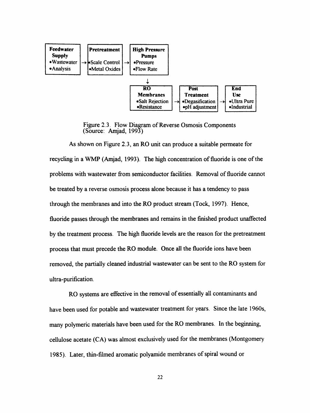
Figure 2.3. Flow Diagram of Reverse Osmosis Components (Source: Amjad, 1993)
As shown on Figure 2.3, an RO unit can produce a suitable permeate for
recycling in a WMP (Amjad, 1993). The high concentration of fluoride is one of the
problems with wastewater fi^om semiconductor facihties. Removal of fluoride cannot
be treated by a reverse osmosis process alone because it has a tendency to pass
through the membranes and into the RO product stream (Tock, 1997). Hence,
fluoride passes through the membranes and remains in the finished product unaffected
by the treatment process. The high fluoride levels are the reason for the pretreatment
process that must precede the RO module. Once all the fluoride ions have been
removed, the partially cleaned industrial wastewater can be sent to the RO system for
uhra-purification.
RO systems are effective in the removal of essentially all contaminants and
have been used for potable and wastewater treatment for years. Smce the late 1960s,
many polymeric materials have been used for the RO membranes. In the begmnmg,
cellulose acetate (CA) was almost exclusively used for the membranes (Montgomery
1985). Later, thin-filmed aromatic polyamide membranes of spiral wound or
22

hollow-fiber arrangements were introduced (Dow, 1997) The specific unit used in the
case study is a BW 30-330 Brackish Water RO element in a spiral arrangement (Dow,
1997). Each element in this system can handle up to 7,500 gallons per day with a sak
rejection of 99.5 percent (Dow, 1997). An example of a spiral-wound RO membrane
is shown on Figure 2 4
FEED
PERMEATE
SPACER
PERMEATE CARRIER
MEMBRANE
Figure 2.4: Spiral Wound Membrane (Source: Gaeta, 1995)
Reverse osmosis incorporates the use of semi-permeable membranes, which
can be easily fouled by some species such as particles precipitating out of solution
while passing through the membranes (Amjad, 1993). The system operates on an
osmotic pressure gradient controlled by the rate at which water and contaminants pass
through the membranes This rate is dependent upon many factors including flow rate
of the wastewater, concentration of contaminants, temperature, pressure, flux, and the
23

pressure, flux, and the design of the specific RO module (Amjad, 1993). For operating
purposes, it is generally the larger particles (ion) that are rejected first. Depending
upon the optimization of the feedwater, RO membranes can last fi-om a few weeks to
more than 10 years (Aurich, 1995). Figure 2.5. illustrates the life span of RO
membranes (Aurich, 1995).
Rate of flux, l/m /h
Start of system
Long term hysteresis
Ufe of a membrane
/(feed, conditiON of feed, and opera
conditions)
^Tlme
Membrane replacement
Figure 2.5: Life Span of RO Membrane (Source: Aurich, 1995)
Factors that can effect the performance of a RO unit include temperature, pH,
changes in pressure, and the flow rate across the membranes (Chang, 1996). The flow
rate across the membrane is proportional to the net pressure across the membrane
24

(osmotic pressure). The following is an empirical representation of the rate at which
sah and water pass through a RO membrane (Clifford, 1985).
Qp = (K^*A)/5 = (AP - AK) = Wp(AP - ATT) Equation (2-4)
H=((Ks*A)/6)*AC = SpAC
Where: Qp = volumetric flow of water, M8= mass flow rate of contaminants (salts), Kw and Kg = membrane permeability coefficients (for water and salts respectively), Wp and Sp = water and sah permeabilhy coefiQcients, AP = hydrauUc pressure difference across the membrane. An = osmotic pressure difference across the membrane, AC = salt concentration difference, A = membrane surface £irea, and
5 = effective membrane thickness (pore size).
Advantages to using a RO membrane process for wastewater treatment are
1. removal of all ions and most dissolved non-ions,
2. responds well to changes in demand (flow and TDS level), and
3. ability to produce ultrapure water.
Disadvantages of an RO system include
1. a high capital cost,
2. the high level of pretreatment required for the RO make-up water (the water that
enters the RO system), and
3. the membranes may foul easily (Montgomery, 1985; Clifford, 1986; Aurich, 1995;
Chang, 1996; and Dow, 1997).
25

2.5 Additional Treatment Options
Other treatment possibiUties considered include evaporation, demineralization,
ion exchange, and contact fihers. Those processes are described briefly in this section,
but were not considered in the final proposal due to either their low ability to
effectively remove fluoride or for economic considerations. These systems are
presented here as alternative treatment processes.
2.5.1 Evaporation
Low-temperature evaporation systems use temperatures of 150 to 160°F to
produce steam; thereby, heating water under a vacuum system (Lindsey, 1993). A
distillation process follows the heating stage leaving behind the unwanted chemicals.
Distillation is an expensive, high energy, consuming process that uses hquid-gas
separation to remove a contaminant fi'om solution (Li, 1992). This is a highly effective
process with proven consistent productive results for the removal of highly
concentrated wastes in a variety of wastewater streams (regardless of chemical
concentration). However, the capital cost is high ($140,000) and requires a high
energy consumption ($20/1000 gallons of treated water) (Lindsey, 1993). Despite its
high efficiency rating, the rate of return on this system («6.9 years) makes it an
unlikely candidate for wastewater treatment in industrial settings where cost reduction
is a bottom line.
26
2.5.2 Demineraliziitinn
Demineralization is a process achieved by ion exchange, membrane processes,
or fi-eezing for an end product of water with no dissolved salts (CUfford, 1986; Li,
1992). Ion exchange methods or absorption (contact beds) are effective removal
techniques for water containing fluoride that needs to have a high removal efficiency,
which leaves a low concentration product (Chfford, 1986). Ion exchange is a selective
removal process for cation and anions whereby wastewater passes through contact
beds containing exchange resins. Most resms can be regenerated and can withstand
thousands of cycles before replacement is required (Clifford, 1986). The beds can be
regenerated when exchange capacities have been met. Ion exchange is used to obtain
higher levels of treatment than obtained by precipitation alone. The downside of ion
exchange methods are the high energy costs associated with the process and the
regeneration of the contact media.
2.5.3 Filtration
In filtration, particles are removed fi-om water as the water percolates through
granular media (Quasim, 1998). This media can consist of many different types of
materials (heterogeneous) or of one material (homogeneous using sand, anthrache,
lecithin, etc.) (Stuart, 1937; Bassett, 1973). The following are examples of absorption
removal techniques used for water containing fluoride:
1. Contact fihers 15" high and filled whh river sand passing a 60 mesh screen
27

mixed with two percent aluminum. Fluoride is removed by the absorptive qualhies of
the sand. The problem with this technique is that the regeneration rate of the sand
leads to a low efficiency rate for the filters and to an eventual solid waste disposal
factor (Stuart, 1937).
2. The second alternative is filter columns filled with clay which has the
capacity to remove fluorides fi-om a level of 1.1 mg/L to 0.46 mg/L The clay had a
high anion demand that correlated to the high cation exchange capacity of the fluorides
for an immediate removal by ion exchange. The downside of this technique is the high
drop in removal in a relatively short period of time. Once the clay meets its holding
capacity for cations, it stops removing them fi^om the wastewater. Regeneration and
sohd waste disposal are two additional drawbacks (Bassett, 1973).
2.6 Disposal of Concentrated Wastewater:
Regardless of the process selected for the treatment process, the by-products
of each process (whether it is coagulation, filter backwash, regeneration wastewaters,
or precipitation) are a small portion of the original wastewater streams, usually around
3 to 10 percent (Quasim, 1998). The disposal of the concentrated wastewater in the
discharge stream falls under the jurisdiction of the Federal Water Pollution Control
Act Amendments of 1972 and EPA fluoride discharge regulations, which specify a 32
mg/L daily maximum and a 17.4 mg/L daily average over a 30-day period for fluoride
m the discharge stream (48 Fed. Reg. 15394, April 1, 1983) (Koblyinski, 1997).
28

The most attractive form of disposal is to the local sanitary sewer system as
long as the concentration of the wastewater does not adversely affect the operations at
the local wastewater municipality (Qasrni, 1998). It has been found at newer
semiconductor plants (buih within the past 5 to 7 years) that the local wastewater
plants have increased treatment efficiency after installation of the recycling system at
the semiconductor facility (Williams, 1997).
Deep well disposal is an additional disposal option. This is a far less attractive
method of disposal and is considerably higher in cost. This disposal method is
regulated by local environmental regulations subject to geological and groundwater
studies. There are several other options that can be used as disposal techniques for
wastewater residual products (Quasim, 1998). Each facility should choose the method
of disposal that best suites their needs.
2.7 Examples of Water Management Programs
Several programs have been launched in the industrial arena to conserve water
and financial resources. The subsequent two sub-sections are brief descriptions of
case studies, their water quality return, and the economic savings resulting fi-om
implementing these treatment plans as a part as water management program. Each
case study is unique but points to the obvious advantages of a WMP. They have been
included in this Uterature review as additional illustrations of the effectiveness of a
WMP on industry.
29
2.7.1 Case Study One
In 1995, a printed circuit board manufacturer began a fiiU scale, reverse
osmosis based WMP. An average return with the WMP was one million gallons of
water each month. This was approximately 65 percent of the facihty's daily water
requirement. This water was recycled at 13 to 30 micro-ohm per cm quahty.^rx Oil Ui ior^ -Ko
/Production at the facility increased 52 percent with the increased quahty of the .
recycled water (Kemp, 1997).^"^^ "^^^^*^^^^ ^ ^ ' ^ ^ CcW^ f) .%^c^
2.7.2 Case Study Two
This study comes fi-om a quick-tum-prototype faciUty that treated and recycled
36,000 gallons of the 100,000 gallons of water consumed each day. The result of this
program was a decrease in disposal cost, higher qualhy water (30 tunes cleaner than
the tap water), 14 million gallons of water saved each year for an annual savings of
$41,000 (Kemp 1997). Water quahty statistics for each of these case studies can be
foui^q^k^on Table 2.4. In addition, the economic savings presented m these two
case studies can be found on Table 2.5.
30

Table 2.4: Water Quahty Statistics for Case Studies One and Two
Flow
TDS
Months of Operation
Feed (gpm) Product (gpm) Recovery (%)
Feed (gpm) Product (gpm) Rejection (%)
Daily Max (gaO Monthly Ave. (gal)
Yearly (gal)
Case Study One
52 23 70
380 7.6 98
76,000 1,000,000
12,000,000
20
Case Study Two
78 70 90
892 24
97.3
100,000 1,160,000
14,000,000
15
(Source: Kemp, 1997)
Table 2.5: Savings Each Year From WMPs at Case Study One and Two
Process
Treatment/Disposal Water Purchase Cost Water Discharge Cost
Water Heating Make Up Water Purification Costs One Time Sewer Access Charge
Future Sewer Access Charge
First Year Savings
Case Study One
33,700 21,400 21,900 31,600 5,400
0 0
114,500
Case Study Two
12,000 9.840
31,160 N/A
7,000 N/A
82,000
82,000
(Source: Kemp, 1997)
31

CHAPTER m
METHODOLOGY
A conceptually based approach was used to develop the water management
program (WMP) presented in this research. Following this section is a case study that
was applied to each of the steps listed in the recommended methodology for the design
of a WMP.
The WMP was approached as a combination of engineering, mathematics,
and chemistry problems with multiple possible solutions, unique in each situation that
it was apphed. Therefore, this is a multiple part problem with multiple possible
solutions. As outlined in this chapter, there are three steps suggested to solving an
engineering problem (see Figure 3.1). These three steps can be applied in the design
of a water management program: identify the problem, analyze and solve the problem,
and present the solution (Wu, 1995). Each step was expanded to describe the
approach which can be applied at any facility wishing to implement a WMP. The first
two steps are the procedural steps used to obtain the solution. The third step is the
presentation of the results, statistical analysis, and an economic evaluation.
Figure 3.1: General Flow Diagram to Solving a Problem
32

Figure 3.1. may appear to be simple, but when the approach is utilized
correctly, the strategy can be eflfective m obtaming a solution to this specific problem.
When each of the subsequent steps (listed below) are followed or altered slightly to
meet specific needs of a facihty, a water management program will be developed.
3.1 Identify the Problem
The first step is to identify the problem or establish a need. There are two
possible problems that can be identified that would initiate the design of a WMP. The
first is when an industrial facility or municipahty is required by law or regulations to
implement a water recycling program for water conservation. T' .e second possible
reason for implementing a WMP is to reduce operating costs and thereby increasing
profit for a company or reducing costs to consumers of a municipahty. This research
concentrates on the economic incentives of implementing a WMP in an industrial
environment rather than the regulatory issues associated with municipalities.
3.2 Analyze and Solve the Problem
This section has three sub-sections for the problem statement in step one.
These sub-sections are a water inventory of the water demands and discharges within
the facility, a sample collection procedure, and an inventory of the contaminants in
each wastewater industrial stream (domestic waste water is not included). The
information in the sub-sections of step 2 are general guidelines and should be tailored
33

to meet the needs of each WMP. The completion of a water inventory is the first task
of step 2.
3.2.1 Water Inventory
The analysis of a facility begins with a detailed water inventory of the high-
water demand areas within the facility. A high water demand for the design of a WMP
will be relative to the total water consumed and discharged from a facility. Therefore,
it will vary for each facihty. For this study, all processes requiring at least 100 gallons
of water per day were considered for the water recychng scheme.
A water inventory is necessary to estabhsh the available water supply for re-use
and/or recycling and can be accomphshed by constructing a chart or spread sheet
showing the processes that require water and their average daily demand. The spread
sheet needs to include additional mformation on the minimum required feedwater
quality and any additional special conditions that a process might require such as
temperature or pressure requirements.
3.2.2 Sample Collection
Samples should be collected fi'om as many possible wastewater streams and
reuse areas that are considered sources for the recycled water. If the water quality
requirements for the reuse areas are already known, this part (Step 3.2.2) does not
need to be followed.
34

Dependmg upon the operating conditions of the facihty for the WMP being
developed, the sampling techniques wiU vary. If the plant operates on a 24-hour, 7-
day a week basis, the samples should be collected as often as possible for as long as
possible within the hmits of physical and economic feasibihty. A seven-day sample
coUection should cover any operation that discharges to the wastewater steam within
the facility. The process engineers or facihty personnel who are famihar with
operations that discharge into the wastewater stream should be consuhed for
information regarding equipment discharge schedules. Once the schedules have been
analyzed, a determination of the necessary number of sample collections can be made
to ensure that the waste fi"om each process is captured at least once during the
collection cycle. It may be found that a seven-day collection interval is too short of a
time schedule to sample each contaminant. The number of samples collected wiU vary
and should be determined by each wastewater producing component m the facility
developing a WMP.
Each sample coUected should be labeled with the location of the sample
stream, time, date, and the name of the person collecting the sample. The she
environmental engineers and safety engineers should be consuhed before the first
sample is ever collected or handled. These engineers should be able to suggest a list of
personal protection equipment (PPE) to be obtained and used during the sample
coUection procedure, transport of samples, and during initial laboratory analysis. The
PPE list might include special equipment or materials for hand gloves, eye protection,
facial shields, protective overcoat, and/or hard hat.
35

Once the sample schedule has been determined, a continuous sampling
technique should be used if at all possible. Since the waste stream is constantly
changmg, a hit-or-miss samphng technique obtamed from grab samples is not as
effective as continuous sampling technique. With the constantly changing wastewater
conditions, rt is easy to miss a contaminant with the hit-or-miss approach. A metered
pump can be used to extract small quanthies of sample continuously for as long as the
samples are scheduled to be collected. A pumping rate of 5 millihters per mmute
should produce a sufficient quantity for a representative sample. Once a sample has
been collected fi'om each wastewater stream, an initial lab analysis should be
performed to obtain baseline information. This information will determine the quahty
and the recycling feasibility of each wastewater stream.
3.2.3 Inventory of Contaminants in Each Stream
Determining what contaminants are actually in each wastewater stream and the
level of concentration is an important step in the WMP. Having the knowledge of
how many contaminants are present and to what range of concentrations are possible
for each one is necessary to determine the treatment needed (next step). Test
parameters should include sahs, metals, conductivity, pH, total sohds, and total
dissolved solids (TDS). A standardized form of testing should be foUowed when each
of these laboratory tests are performed. Standards Methods manual or guidelines set
by the EPA should be consuhed when plannmg the laboratory analysis (Mollhagen,
1995).
36

Additional precautions should be taken when working whh wastewater of
unknown strength, chemical composition, or hazardous potential. The same PPE
required for the sample collection should be worn by persons handling the wastewater
in the laboratory until the composhion of the waste can be determined and a new
protocol established.
3.3 Presentation of Alternative Solution(s)
As h was stated in the first paragraph of this chapter, there is the possibihty of
more than one solution to the problems faced while designing a WMP. In the
industrial world, cost is generally the prime criterion. However, cost is secondary to
technical feasibility because if an operation can not perform to the desired level then
cost is not significant. Once all the available treatment options have been explored, the
most cost-effective solution should be presented for implementation. In some cases,
there may be regional factors affecting cost (available supplies, space, energy cost,
etc.). This step has three sub-sections: statistical analysis, exploration of treatment
options, and economic evaluations. The available treatment options must be sized
before an economic evaluation can be determined.
3.3.1 Statistical Analysis
A statistical analysis is necessary in development of the WMP to determine the
quality of the wastewater available for implementation of the program. The treatment
goals should be set to those concentrations of the existing water supply, since h is that
37

supply that would be replaced in the hnplementation of a WMP. There are three steps
to foUow in the statistical analysis. Those are:
1. Determine the most efficient sample collection protocol for the
wastewater in the case study. This is a calculation of the rehabihty and confidence
level of the analysis for the three sample sets collected. This determines which sample
set is the most rehable of the sets collected.
2. Determine the quality of the data set that was deemed the most reliable form step 1
of this section. This is to ensure that the data falls within acceptable quahty control
limits. The quality control limits are estabUshed by the distance (standard deviations)
the values are from their mean value. Data outliers are discovered in this process.
This is not a comparison of the sample set to any other samples, but an internal
analysis of samples within the data collection set to determine the qualhy of the
collection method (not the quality of the sample).
3. Once the data has been deemed the most rehable of all the samples
collected and it is acceptable within quality control measures, the next step is to
determine the relationship between hs qualhy and the goal concentrations (in this case,
the tap water) for the treatabihty study. This determines the quality of the sample.
Any contaminant in the wastewater stream that is of higher quality or whhin
plus one standard deviation from the mean of the existing water supply is considered
to be of good quality. Any contaminant falling beyond plus three standard deviations
from the goal concentration is labeled poor and should be considered with the target
elements in the treatment step of the WMP. The statistical operations used to
38

determine steps 1, 2, and 3 of this section are the central tendencies (mean, median,
and mode), standard deviations, rehability, and the Pearson Product Moment
Correlation Coefficients.
3.3.2 Treatment Options
The first procedure in exploring the treatment options is to determine the
quahty desired in the final end product. This will have the largest unpact on
determining the necessary treatment sequence. Once the desired quality has been
estabhshed, single out the target elements in the wastewater stream supplying the
water for the recycling process. The target elements are those elements or complexes
that would potentiaUy foul addhional processes further do vn the treatment line. For
example, if the desired end product is ultrapure water (as in the semiconductor
industry), a membrane separation unit should be considered as the final treatment stage
to obtain this water quahty level if the preceding treatment processes can not obtain an
acceptable water quality level. For example, if the wastewater contained chlorides or
fluorides, these components would foul the membranes of an RO unit and would
therefore be labeled as target elements (US Filter, 1997).
Current journals and other professional Uterature on wastewater treatment and
contaminant removal process should be explored for possible treatment options.
Previous studies on similar projects relating specifically to the operations of the faciUty
desiring a WMP should be examined as weU. Some industries have networking
associations for sharing information on projects that they have previously worked on
39
or are currently involved. Consult professionals within the appropriate discipline for
mformation regarding how to contact these organizations or for advice on how to
approach the treatment process.
3.3.3 Economic Evaluation
Once suitable treatment options have been identified, the Ust can then be
narrowed down to two or three selections based on economic considerations. This is
an hnportant step in WMP selection because a project must be profitable to an
institution in order for the program to be implemented (with the exception of
mandatory regulations). There are several methods to evaluating a process
economically. Information on previous operations can be used with the current design
parameters (flow rate, pH, TDS, etc.) and the life expectancy of the system to come
up whh an economic evaluation. A comparison can then be made among the final
economic evaluations of these processes to make the final decision on which treatment
process to be implemented.
The Present-Worth Method can be used to determine the economic benefits or
costs of a process to the WMP. It is important to consistently use the same constants
in the economic formula for such factors as the interest rate, time period of economic
value (use a salvage value of equipment if necessary), and a consistent risk factor.
This subscribes to the four basic rules of cost-benefit analysis that are as foUows:
1. Figure aU cost-benefit ratios by using the same discount (interest) rate.
40
2. Clompare aU alternatives over the same period of analysis.
3. Calculate the cost-benefit ratio for each alternative. Choose aU alternatives having
a cost-benefit ratio exceeding unity. Reject the rest.
4. Rank the alternatives in the set of mutuaUy exclusive alternatives m order of
increasmg costs. Calculate the cost-benefit ratio using the incremental cost and
incremental benefit of the next alternative above the least costly alternatives.
Choose the more costly if the incremental cost-benefit ratio exceeds unity.
Otherwise, choose the less costly alternative. Continue the analysis by considering
the alternatives in order of increase cost, the alternative on the less costly side of
each increment being the most costly project chosen thus far (James and Lee,
1971).
Some computer programs are avaUable such as WW Cost by CWC
Engineering Software for calculatmg the present worth of a treatment process.
Otherwise, calculations can be made by hand.
3.3.4 Overview
1. Estabhsh a need for recycUng withm a facUity, and then determme which
wastewater streams are available for recyclmg based on quahty and quantity.
2. A baseUne data base should then be compUed to determine the most feasible
wastewater sources for recycUng.
3. Addhional samples should be coUected fi-om the wastewater streams that will be
the primary sources of recycled water.
41

4. Data fi'om the additional coUections is used to determine variations and peaks
within the supply.
5. Comparisons are then made whh the supply stream to goal concentrations set by
the existing supply stream (tap water).
6. Treatment options are explored to remove sufficient levels of the contaminants to
loop the treated wastewater by into the existing receiving stream for the faciUty.
7. A water management program can then be proposed and presented for
implementation.
42

CHAPTER rV
SITE SPECIFIC CASE STUDY
The general procedures of designing a WMP (as discussed in Chapter III,
Methodology) were applied to a local semiconductor facility for the case study
evaluated in this study.
4.1 Identification of Case Study Problem
The problem addressed in this case study, was estabUshing a need and
identifying economicaUy and technologically feasible solutions for recycled water
through the facility. The need for recycled water was based on economic incentives to
reduce operating costs, to decrease water discharge and purchase costs, and to
increase operational efficiency. A flow chart (Figure 4.1) was constructed to foUow
during the various decision stages of designing the water management program.
EconomicV Yes /Alternatives Yes / Process \ Yes Feasibility] > > >( Cheapest?) > > >V Refinements j-»-^—)| Design
Completed^/
Noi
Pilot Study
t t T
-» » > > T
Figure 4.1: Case Study Logic Flow Chart (Source: Montgomery, 1995)
43

Included in the identification of the case study problem was a definition of the
experimental procedures, level of technology in use and available, and the
experimental parameters. Each of these parameters are important to better understand
and evaluate the identified problem, after which, the problem can be analyzed and a
solution formulated.
4.1.1 Experimental Procedures
Industrial wastewaters are constantly changing in terms of chemical waste
concentrations. Treatability studies were conducted beginning with laboratory tests
for the purpose of translating experimental data into design and operational
parameters. The first step was sample coUection foUowed by laboratory analysis. A
total of three sample collection techniques were used. Finally, statistical and
economical analyses were conducted to determine the process with the best potential
for energy efficiency and revenue return.
4.1.2 Level of Technology
In the case study, the industrial plant is operating 24-hours a day, seven-days a
week. The waste produced is segregated into an industrial waste stream and an acid
waste stream. The industrial waste stream was the primary focus. This waste is
collected from an accessible pump/lift station where aU industrial waste lines termmate.
The combined wastewaters are then pumped out for treatment and final discharge
from the plant. It was found not to be economical or time permissible to segregate the
44
waste Unes contributing to this hft station for sample collection, based on man hours
and the potential hazard firom breaking lines. Therefore, samples were collected from
the sump at the wastewater lift station.
4.1.3 Experimental Parameters
It was estimated that each plant operation contributing to the final industrial
waste stream (primarily those within the wafer fab) would dump waste at least once
every four hours. The hft station, where the waste streams came together and samples
were coUected, pumped continuously at a rate based on the volume of the wastewater
within the tank. Therefore, h was determined that the most accurate form of sample
coUection would be a continuous sample coUection operation. This, however, is not a
possible option as the equipment and man-hours were not available for this project.
Therefore, with each of the following listed factors considered, the first set of samples
were coUected every hour during a 24-hour samphng period.
1. Plant operations contributmg to the final industrial waste stream dump at least
once every four hours. It is desired that each constituent and its concentration in
the waste stream be sampled at least one time during the mterval.
2. Sample coUection required approximately 20 minutes.
3. Lab analysis for each sample was estimated at one hour (for analyzing samples in
triplicate). Metals, salts, TS, and TDS were all analyzed at the parts-per-nuUion
level. Conductivity and pH were also included in the lab tests.
45

4.2 Analysis of the Case Study Problem
The analysis of the-how-to-approach the water management program began
with meetmg three objectives: a water inventory, sample coUection, and an inventory
of the contaminants in each of the samples. Once these objectives had been met, a
solution could be formulated to design the WMP.
4.2.1 Water Inventory
The water inventory was the fhst step in estabUshing a need for recycling water
within the faciUty. Therefore, a water inventory was made of the high water demand
operations whhin the facUity. Those areas are Usted on Table 4.1.
Table 4.1: Approximate Water Inventory
Process Scmbbers
Coolant Towers (North) Coolant Towers (South)
DI Plant
# Units 9 11 6 1
Demand per Unit 10-15gpd 5500 gpd 2700 gpd 150 gpd
Sut3total 135
60500 16200 150
(Source: Hector, 1997)
The operations listed are not aU inclusive of every process or operation whhin
the plant that requhes water. However, they are major supply and demand areas. The
water demand for these processes alone comes to almost 77,000 gpd. This is the
amount of water purchased and discharged on a daUy basis. Thus, when the water
demand of these operations are combined, they create a major contribution to the
recycling process.
46
4.2.2 Sample Collection
The first step was to construct a plan to determine which areas of the facUity
samples would be coUected. Safety requhements and Standard Methods (method
300.0), techniques were foUowed for coUectmg the samples. The mdustrial
wastewater whhin the facUity faUs into one of three categories: acid wastewater,
industrial wastewater, or water from the DI plant.
To best represent the water being evaluated and sufficient quantities collected
for analysis; aU major contributing water and wastewater supply lines, the two main
wastewater Uft stations, and several lines fi'om the DI plant were tested to determine
the quahty of the avaUable water supply. Initial samples were coUected from each
main industrial and acid wastewater stations and lines on random days and times over
the course of six months (see Figure 4.2). These initial samples were used to create
an overview and baseline of the contaminants present in the industrial and acid
wastewater supply. The wastewater within this faciUty feU into ehher the acid or
industrial waste category.
Both the EPA and Standard Methods procedures recommend the use of ehher
polyethylene or glass containers for coUection and transport of materials that could
contam hazardous contents such as those in the wastewater streams presented in this
case study. Therefore, each sample was coUected, transported, and stored in
sterilized, polyethylene bottles (150 and 500 ml). In addition, the EPA guidelines
recommended that samples were not stored for more than 28-days (14-days for
Nhrate-N, non-chlorinated water) before lab analysis could be conducted. In
47

following these guidelines, tests were performed withm one week of theh coUection
date.
Since hazardous and/or corrosive materials were possible in either of waste
streams, a hazardous condhions plan was constructed by the she's safety engmeer.
The plan included the recommendation of using personal protective equipment (PPE):
safety glasses, face shields. Tan Tionic® gloves over gray 4H gloves, gray 4H apron,
and gray 4H sleeves. Any disposable material that contacted the waste material was
disposed of within 30-minutes of use. The foUowing is a Ust of the locations within
the semiconductor plant where samples were initially collected.
1. Incoming Tap Water 2. Industrial Waste Tank No. 2 3. RO Brine 4. RO Product 5. ROMake-Up 6. Recycled DI 7. Industrial Waste Lift Station 8. 125 mm Scrubber
9. 150 mm Scrubber 10. TLM Scrubber 11. Acid Waste Lift Station 12. Wet Processes 1, 2, and 3 13. Wet Processes 4 and 5 14. Lateral One 15. Clean Up Shop
Figure 4.2: Sampling Shes Whhin the Facility
On November 26, 1996, samples 1 through 10 were coUected and analyzed.
On December 10, 1996, samples 1 through 6 were collected and analyzed to confirm
the initial set of data. A more specific analysis was necessary to locate point source
pollution areas. Therefore, on June 15, 1997 samples 2, 5, 7, and 11-15 were
collected and analyzed agam. It was evident at this point that there would be ample
areas fi"om which wastewater could be recovered and coUected that was of treatable
quality within the facility to treat and recycle.
48

The wastewater in each line contributing to the lift stations flows under
gravitational forces. It was important to segregate mdividual Unes contributing to the
acid lift station, as the waste contained there was strong and highly concentrated. If
mformation could be obtained that would mdicate which Ime or Unes contributed a
higher concentration of waste to the final waste stream, then that would allow
rerouting of one or more of these Imes so that the remaining volume of wastewater
could be used for recycling purposes. There are four main lines that contribute to and
come together at the acid lift station. Those four acid wastewater lines are on Figure
4.2. shown below.
Lateral Line #1
i Wet
Processes 4 &5
i Wet
Processes 1,
i Acid Lift Station
2, &3 Ciean-Up
Shop
i
Figure 4.3: Acid Wastewater Flow Scheme
The combined flow rate out of the acid lift station is a small quantity compared
with the flow out of the industrial lift station. After laboratory analysis of the
segregated acid wastewater lines (Table 4.2), h was determined that the strength and
concentration of the acid wastewaters (in part due to the decrease in dUution resuhing
in an overaU smaller volume) would be too high to treat and recycle at an economic
rate.
The wastewater lines that contributed to the industrial hft station could not be
segregated as easily as the acid lines. They are more numerous in number and have
49

Table 4.2: Acid Wastewater Analysis
Sample
Acid Line 1
Acid Line 2
Acid Line 3
Acid Lift Station
Fluoride
ppm
213 900
63 9 465
Chloride
ppm
171 595
ND NO
Nitrate
ppm
ND ND
ND ND
Sulfate
ppm
14416 16517
6 15928 13180
Sodium
ppm
8776 15847
41038 40557
Potassium
ppm
8522 16684
37527 25034
Calcium
ppm
9101 9246
14579 18203
Iron
ppm
6148 3583
6454 5922
pH
1.20 1.10
1.20 1.60
many coimecting points. Therefore, they are not individuaUy represented, but are
represented as one wastewater stream that contributes to the final product at the point
of the mdustrial Uft station. It is not necessary to show the Unes contributing to the
mdustrial lift station, as the wastewaters are not as concentrated. The general flow of
the existing mdustrial and acid wastewater within the faciUty and the discharge from
the plant can be seen in the flow diagram (Figure 4.4).
Acid Lift Station
i-
Industrial Lift Statior
-i
i Addition of Caustic
Discharge to City Wastewater Treatment Plant
Figure 4.4: General Wastewater Flow Scheme
Three sample collection techniques were used to determine a comprehensive
analysis of the wastewater stream. Those three techniques were:
50

1 A 24-hour sampling period, in which samples were collected every hour (on the
hour) for 24-hours for a total of 24 samples. Grab samples were collected with a
hand-held pump inserted in the center of the industrial waste tank approximately
halfway from the water surface. This approach was a hit-or-miss technique and
had a low probability of returnmg reliable data. This sample collection set will be
referred to as data set A
2. In hopes of increasing accuracy, a second approach utilized a metered pump
secured over the center of the tank with the intake tubing anchored near the
bottom of the tank. Samples were continuously pumped out at an approximate
rate of 5 ml per minute and composite samples were collected every thirty minutes.
The coUection continued for 24-hours for a total of 48 samples. The reliability of
the data was expected to increase over that of the first technique due to the
continuous samphng approach even though analysis was not instantaneous. This
collection technique was used to gather data continuously over one randomly
selected day. This data set will be referred to as data set B.
3. The third set of samples were collected utilizing the second approach of
continuous samphng whh a metered pump but over seven consecutive days.
Samples were continuously pumped at an approximate rate of 5 ml/minute for each
24-hour period and then composite samples were collected at the end of each 24-
hour period. This technique gave a total yield of seven samples. These samples
were collected to examine the variance and central tendencies from a day-to-day
stand point. This data set will be referred to as data set C.
51

4.2.3 Inventory of Wastewater Contaminants
Metals and salts were the two primary categories of analysis. Metals in water
and wastewater range in their effects on treatment processes and the surrounding
environment from beneficial to dangerous. Dissolved inorganic contammants can be
amphoteric, neutral, cationic, or anionic forms of ions, atoms, or particles of any
element in the periodic table. The first step in testing each sample was an analysis for
fluorides, chlorides, nitrates, and sulfates using a Dionex Ion Chromatograph series
40001 with Al-450 software. Each sample was then tested for metals including Na, K,
Ca, Fe, Mg, Ni, Zn, and Sn (among other metal elements) usmg atomic mass
absorption methods.
To complete the lab analysis, each sample was tested for conductivhy, pH,
total dissolved sohds, and total solids. Each data set coUected from December 1996 to
October 1997, was analyzed by each of these methods. A comprehensive analysis of
all of these lab tests was used to obtain a wastewater quahty level of the industrial
waste. Qualitative characteristics were necessary to determine the most cost-effective
and cost-beneficial treatment process.
4.2.3.1 Sah Analysis
Total dissolved solids (TDS) is the sum of the dissolved salts in solution.
Therefore, the samples were first analyzed for salt contents. In this group, fluorides
created a specific problem in the treatment process. The most electronegative of aU
52

the elements, fluoride is almost always combined whh other elements when found in its
natural envhonment (Onuoha, 1983).
The POTWs that supply the water used in this case study produce a water
supply that meets the U.S. PubUc Health Source Drinking Water Standards mandatory
limit for aUowable fluoride. This pretreatment goal is to reach this level of fluoride
concentration or the maximum permissible concentration (as noted by the membrane
manufacturer) in the mdustrial waste before sending h to the RO system. Salt levels
for each of the sample sets coUected are found on Tables 4.3, 4.4, and 4.5.
4.2.3.2 Metal Analysis
Hardness of the water is the sum of the dissolved iron, dissolved manganese,
calcium, and magnesium. Sodium, potassium, calcium, and hon were the primary
dissolved inorganics of concern in the industrial wastewater. In this case, hon was the
only constituent that peaked over the city concentration regulations. The hon level
was close to the regulation level and does not pose serious treatment problems as does
fluoride. The metal analysis for each of the samples collected can be found on the
following pages on Tables 4.6, 4.7, and 4.8.
4.2.3.3 Addhional Analysis
Each of the samples were then analyzed for pH, conductance, TDS, and TSS.
The coUection of these chemical and physical parameters were used to better
determine the appropriate treatment process or series of processes.
53

Table 4.3: Sah Analysis for Data Set A
Sample
Time
700
800
900
1000
1100
1200
1300
1400
1500
1600
1700
1800
1900
2000
2100
2200
2300
2400
100
200
300
400
500
600
Salts (ppm)
Fluoride
69.3
68.6
60.9
6.36
8.93
9.71
22.6
78
8.79
4.36
20.4
75
5.8
17.8
5.03
14.1
12.9
35.2
18.1
8.46
22.4
3.81
21.8
15.6
Chloride
43.9
43.7
297
28.9
24.4
36.3
224
50.7
38.6
101
48.9
46.5
89.2
58.5
31
39.3
39.1
56.8
207.7
38.6
92.6
40.6
42.7
51.8
Nitrate
0
0
0
0
0
0
0
0
0
0
2.99
0
0
2.77
0
0
0
3.29
0
2.92
0
0
0
2.52
Sulfate
113
113
42.3
15.9
22.1
76
136
66
35.4
28.3
212
34.9
36.9
136
17.6
54.9
52
47.2
34.2
113
79.7
26.8
75.8
44.5
54

Table 4.4: Salts Analysis for Data Set B
Sample Time 700 750 800 850 900 950 1000 1050 1100 1150 1200 1250 1300 1350 1400 1450 1500 1550 1600 1650 1700 1750 1800 1850 1900 1950 2000 2050 2100 2150 2200 2250 2300 2350 2400 2450
Salts Fluoride
14.19 15.54 11.74 9.95
21.99 18.69 12.03 15.22 25.00 27.54 28.34 23.31 28.68 39.88 41.97 10.28 18.85 21.49 31.73 30.51 29.41 10.26 21.03 10.87 7.57 12.18 6.53 18.61 11.67 16.19 12.50 12.30 11.19 18.11 15.45 13.25
Chloride
40.97 182.36 42.83 40.86 96.95 52.67 48.70
208.23 40.50 36.05 54.19 42.16 51.93 43.15 44.93 48.93 273.96 38.43 164.86 70.20 53.47 55.00 63.05 75.46 67.19 79.42 43.78 41.60 38.05 43.51 32.69 43.32 56.43
284.33 199.03 56.80
Nitrate
0.00 0.00 0.00 0.00 0.00 0.00 0.00 2.71 0.00 0.00 0.00 0.00 0.00 0.00 14.14 0.00 0.00 0.00 3.72 0.00 0.00 0.00 0.00 0.00 0.00 0.00 0.00 0.00 0.00 0.00 0.00 0.00 0.00 0.00 0.00 0.00
Sulfate
62.05 164.76 133.84 83.20 73.59 76.42 55.94 49.59 89.80 85.04 77.91 61.26 50.24 74.35 74.00 54.56 87.18
211.60 120.68 102.35 72.14 99.55 74.03 56.88 76.30 167.53 51.78 41.08 53.05 79.69 48.30 93.46 99.46 136.73 86.08 105.02
Phosphate
5.11 1050.41 21.69 15.62 7.59 9.14 7.74 6.83 6.28
28.08 18.98 6.20 0.00 0.00 5.36
554.81 5.50 8.66
24.02 0.00
21.86 4.15 15.67 20.03 1298 24.89 6.18 11.82 14.59 18.03 28.99 22.10 40.93 14.66 8.26
875.14
55

Table 4.4: Salts Analysis for Data Set B (Contmued)
Sample
Time
100
150
200
250
300
350
400
450
500
550
600
650
Salts
Fluoride
17.77
25.70
16.90
23.29
6.71
11.56
12.27
14.04
17.00
5.29
12.76
12.26
Chloride
66.86
110.36
47.51
48.39
51.95
33.06
60.65
44.40
44.96
115.18
177.54
55.64
Nitrate
4.47
0.00
0.00
0.00
0.00
0.00
0.00
2.87
0.00
0.00
0.00
0.00
Sulfate
78.75
58.60
108.32
92.95
107.14
127.14
103.65
73.94
44.31
159.43
289.87
94.58
Phosphate
1271.53
123.45
74.86
31.09
25.14
180.93
443.48
121.21
52.80
51.97
27.91
138.20
Table 4.5: Salts Analysis for Data Set C
Sample
Time
1
2
3
4
5
6
7
Salts
Fluoride
31.7
38.9
66.2
47.7
21.8
61.6
58.6
Chloride
85.7
121.8
91.2
139.6
92.1
107.9
99.9
Nitrate
0
0
0
0
0
5.099
0
Sulfate
102.2
103.1
85.8
121
96.4
132.1
111.7
Phosphate
185.2
82.6
112.6
103
127
110.5
173.2
56

Table 4.6: Metals Analysis for Data Set A
Sample
Time
700
800
900
1000
1100
1200
1300
1400
1500
1600
1700
1800
1900
2000
2100
2200
2300
2400
100
200
300
400
500
600
Metals
Na
20.9
21.5
1.35
15.2
9.1
15.3
17.9
18.9
23.4
17
49.2
24.4
20.7
59.7
13.3
21.5
39.6
57.6
28.1
26.4
27.5
24.6
28.4
50.9
K
0.411
0.335
0.00937
0.108
0.149
0.378
0.331
0.361
0.347
0.309
0.369
0.39
0.419
0.529
0.355
0.484
0.579
0.581
0.479
0.531
0.494
0.568
0.536 0.574
Ca
3.55
3.59
0.146
0.727
0.331
3.2
3.83
4.07
3.76
3.37
4
4.33
3.96
4.57
2.59
447
6.33
5.23
4.67
5.23
5.02
5.57
5.18 5.74
Fe
2.33
2.35
0.0972
0.463
0.245
1.99
2.51
2.57
2.34
2.09
2.51
2.62
3.25
3.73
2.07
3.62
5.1
4.04
3.76
4.12
3.96
4.57
414
4.53
57
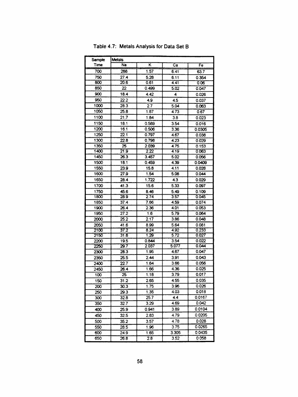
Table 4.7: Metals Analysis for Data Set B
Sample Time
700 750 800 850 900 950 1000 1050 1100 1150 1200 1250 1300 1350 1400 1450 1500 1550 1600 1650 1700 1750 1800 1850 1900 1950 2000 2050 2100 2150 2200 2250 2300 2350 2400 2450 100 150 200 250 300 350 400 450 500 550 600 650
Metals Na
288 27.4 20.6 22
18.4 22.2 28.3 25.8 21.7 18.1 16.1 22.1 22.8 25
21.9 26.3 18.1 23.9 27.9 28.4 41.3 45.6 28.9 37.4 26.4 27.2 25.2 41.6 37.2 31.6 19.5 29.7 28.3 25.5 22.7 26.4 25
31.2 30.3 29.3 32.8 32.7 25.9 32.5 35.2 28.5 24.9 26.8
K
1.57 5.28 0.61
0.499 4.42 4.9 2.7 1.87 1.84
0.589 0.506 0.797 0.798 2.039 2.22 3.457 0.459 15.8 1.54 1.722 15.6 8.46 2.74 7.66 2.36 1.6
2.17 8.99 8.24 1.29
0.844 2.037 1.95 2.44 1.64 1.66 1.18 2.65 1.75 1.35 257 3.29 0.941 2.83 3.57 1.96 1.65 2.8
Ca
6.41 6.11 4.41 5.02
4 4.5 5.04 4.73 3.8
3.54 3.36 4.67 4.23 4.75 419 5.02 439 411 5.06 43 5.33 5.49 3.57 4.59 401 5.79 3.86 5.64 4.92 5.72 3.54 5.077 4.67 3.91 3.66 436 3.79 455 3.96 403 4.4 469 3.89 4.79 4.78 3.75 3.305 3.52
Fe
63.7 0.354 0.06 0.047 0.026 0.037 0.063 0.67 0.023 0.016 0.0305 0.038 0.029 0153 0.063 0.056 0.0409 0.028 0.044 0.029 0.097 0.109 0.045 0.074 0.053 0.064 0.048 0.081 0.233 0.027 0.022 0.044 0.047 0.043 0.056 0.025 0.017 0.035 0.026 0.018 0.0167 0.042 0.0104 0.0205 0.028 0.0265 0.0435 0.058
58

Table 4.8: Metals Analysis for Data Set C
Sample
Time
1
2
3
4
5
6 7
Metals
Na
33.6
31 36.4
49
29
42.1 60.1
K
0.706
0.643
0.525
1.52
0.557
0.712
0.657
Ca
4.53
4.31 3.67
11.3
4.08
5.096 4.303
Fe
0.027
0.00102
0.015 0.00247
0.035
0.0468 0.0594
pH was the first parameter analyzed in this section. This parameter can change when
exposed to air and therefore was measured soon after samples collection. Since the
majority of the samples collected were in lift stations and the lift stations are open to
the atmosphere and under turbulent conditions, less concern was raised over the pH
changes fi-om exposure to the air. The analysis can be found on Table 4.9 and 4.10.
59

Table 4.9: Conductance, pH, and TS for Data Set B
Sample
700
750
800
850
900
950
1000
1050
1100
1150
1200
1250
1300
1350
1400
1450
1500
1550
1600
1650
1700
1750
1800
1850
1900
1950
2000
2050
2100
2150
2200
2250
2300
2350
2400
2450
Conductance
(micro-ohms)
0.465
3.4
0.81
0.46
0.691
0.582
0.397
0.976
0.604
0.557
0.69
0.451
0.492
0.562
0.568
1.245
2.23
1.11
1.26
0.624
0.683
1.29
0.604
0.614
0.621
1.48
0.395
0.421
0.367
0.541
0.359
0.544
0.615
2.11
1.54
1.6
pH
9.4
2.4
3
4
5.6
9.1
4.3
3.5
9.6
6.1
8.3
3.9
3.6
3.5
3.5
2.8
2.5
2.9
2.9
3.2
3.2
2.7
9.1
10.1
9.1
2.6
9.7
8.9
3.9
9.3
3.8
9.2
7.7
2.6
2.7
2.8
Total Solids
(mg/L)
231
1114
500
440
480
242
180
358
262
244
212
242.5
242
294
292
780
660
464
428
242
244
336
204
244.7
235.6
426
218
172
202
246
260
246
276
614
460
1186
60

Table 4.9: Conductance, pH, and TS for Data Set B (Continued)
Sample
100
150
200
250
300
350
400
450
500
550
600
650
Conductance
(micro-ohms)
2.53
0.866
0.656
0.551
0.541
4.38
1.44
0.737
0.482
1.48
1.69
2.33
pH
2.4
8.7
3.3
6.8
8.7
2
2.2
2.6
94
7,7
2.6
2.9
Total Solids
(mg/L)
1672
310
314
226
252
2554
772
340
190
498
692
1738
Table 4.10: Conductance, pH, and TS for Data Set C
Sample
1
2
3
4
5
6
7
Conductance
(micro-ohms)
0.882
0.891
0.889
0.987
0.772
1.043
1.009
pH
3.45
3.28
3.43
3.36
3.59
3.23
3.18
Total Solids
(mg/L)
510
444
452
486
442
476
534
4.3 Presentation of Solution
The solution begins whh a statistical analysis of the collected data samples. It
is then followed by explormg the available treatment options. When the treatment
options have been identified, an economic analysis is performed to determine which is
the most cost-beneficial to implement.
61

4.3.1 Statistical Analysis
The statistical analysis is a mathematical process of describmg the wastewater
quahtatively at specific pomts in time to determine the rehability if each sample set and
technical feasibility of treating the samples m the case study. In performing a
mathematical analysis, the confidence level of the collected samples increases.
Therefore, the constituents in each sample were analyzed for central tendencies (mean,
median, and mode), quahtative characteristics usmg variabihty (standard deviation),
and Pearson analysis. Also, a calculation was made of the data's confidence/rehability.
The statistical analysis is Step 3.1 (Chapter lU) in the general procedures of
designing a WMP. The three sub-steps in that section were foUowed in the case study
to determme the quahty of the samples and theh required treatment level with respect
to the quahty goal set by the current tap water supply. Step 1 was to determine which
sample coUection method provided the most reliable data. This was done whh a
rehability and confidence analysis.
4.3.1.1 Accepting Sample Collection Sets
Determinmg the rehability of the data played a large role in whether or not the
sample sets were considered vahd. Validity is important in the research process for
scientific credibility. Therefore, mathematical calculations were used to indicate the
rehability sample sets. The resuhs were accepted or denied based on a range of values
for the required quality, testing ability, and senshivhy analysis. Johnson (1994) defines
rehabUity as "the probability that h wiU fimction within specified limits for at least a
62

specified period of time under specified environmental condhions" (p. 549). In this
definition, "it" apphes to the data set coUected and the environmental conditions refer
to the operating conditions that the samples were coUected under. This mcluded
condhions that were not considered optimal, such as peaks in operational discharges.
Therefore, all conditions, high or low, were taken into consideration.
The rehabihty of the collected data was calculated whh a computer-aided
program (Excel ®, Windows 95 ®). The following calculations can be performed by
hand if a computer program is not available.
Rehabihty (Equation 4-1) oc 0.85 0.90 0.95 0.99 N (3*5^8 ^ (3*5^)/s^+2 (3*5^)/e^+3 (3*5^)/s ^+4
Where: ai=[(nSxi'-(Ixi) 0/(n*(n-l ))]^. 5 N=(t')*(6^/8^) ReliabUity ( r ) > 50% 6= standard deviation e= tolerance of utUized equipment t= student's distribution and rehabihty table N= Number of tests x= percentage of rehabihty (Cohen, 1979)
The data on Table 4.11 can be used to determme the most rehable sample
coUection method. These values indicate the samples' reliabUity whhm each
percentage range. The lower the value on Table 4.11 for each constituent, the smaller
the distance that value is fi-om the mean for that contaminant (within that particular
percentage of rehabUity). As the reliability increases (85 percent^90 percent->95
percent), the values on the table decrease. This is because the distance fi'om the mean
decreases (Gilman, 1997). The smaller the value calculated for each percentage range,
63

the higher the reliabUity. Therefore, when makmg comparisons of the reliability
between the three data sets (A, B, and C), the smallest value for each percentage range
exhibhs the best rehability. This was the procedure followed to identify the most
reliable sample coUection set.
From Table 4.11, data set C has the highest reliabUity. Therefore,
the sample collection information fi'om this will be used m the subsequent
statistical analysis step.
Table 4.11: Rehabihty Levels of Data Sets A, B, and C
Data Set (C): 24-Hr sampling, 7 day period (9/26/97-10/3/97)
Reliability (0.85)
Reliability (0.90)
Reliability (0.95)
Reliability (0.99)
Metals (ppm)
Na
3.70
5.70
6.70
7.70
K
0.00
2.00
3.00
400
Ca
0.21
2.21
3.21
4.21
Fe
1.47E-05
2.00
3.00
4.00
Salts (ppm)
Fluoride
8.27
10.27
11.27
12.27
Chloride
11.17
13.17
1417
15.17
Nitrate
0.11
2.11
3.11
411
Sulfate
7.21
9.21
10.21
11.21
Phosphate
42.64
44.64
45.64
46 64
Data Set (A): 24-Hr sampling (0700 8/8/97 • 0600 8/9/97)
Reliability (0.85)
Reliability (0.90)
Reliability (0.95)
Reliability (0.99)
M^als (ppm)
Na
6.62
8.62
9.62
10.62
K
0.00
2.00
3.00
4.00
Ca
0.08
2.08
3.08
4.08
Fe
0.06
2.06
3.06
4.06
Salts (ppm)
Fluoride
18.36
20.36
21.36
22.36
Chloride
144.76
146.76
147.76
148.76
Nitrate
0.04
2.04
3.04
4.04
Sulfate
69.50
71.50
72.50
73.50
Phosphate
Data Set (B): 24-Hr sampling (0700 9/12/97 - 0650 9/13/97)
Reliability (0.85)
Reliability (0.90)
Reliability (0.95)
Reliability (0.99)
Metals (ppm)
Na
43.55
46.55
46.55
47.55
K
0.66
2.66
3.66
4.66
Ca
0.02
2.02
3.02
4.02
Fe
2.53
4.53
5.53
6.53
Salts (ppm)
Fluoride
2.09
4.09
5.09
6.09
Chloride
113.84
115.84
116.84
117.84
Nitrate
0.15
2.15
3.15
415
Sulfate
63.42
65 42
66 42
67.42
Phosphate
2219.52
2221.52
222252
2223.52
64

4.3.1.2. Determinmg the Quahty of Sample Sets
The second stage of the statistical analysis was determmmg the quahty of the
selected sample set C. This was done to ensure that the set feU whhin acceptable
quahty control (QC) hmits. Just because the sample set was selected as the most
rehable of the three sets, hs rehabUity did not indicate that h was also whhin QC Ihnits.
If all three of the samples had been outside the QC hmits, then the set selected
as most rehable of the three stUl would not have been very dependable. Therefore,
conventional quahty control charts were prepared for each of the consthuents in
sample set "C." The data pomts used to construct the QC charts can be found on
Table 4.12.
Table 4.12: Conventional Quality Control Data for Sample Set C
standard Deviation
From the mean
Mean
Standard Deviation
(+) 1 (good)
(+) 2(accept.)
(+) 3 (poor)
(-) 1 (good)
(-) 2 (accept.)
(-) 3 (poor)
Metals
Na
40.17
11.10
51.30
62.40
73.50
29.10
18.00
6.90
(ppm)
K
0.76
0.34
1.10
1.44
1.79
0.42
0.08
-0.27
Ca
5.33
2.67
7.97
10.60
13.31
2.66
0.00
-2.67
Fe
0.03
0.02
0.05
0.07
0.09
0.00
-0.02
-0.04
Salts (ppm)
Fluoride
46.64
16.60
63.20
79.80
96.40
30.00
13.40
-3.20
Chloride
105.46
19.30
124.80
144.10
163.40
86.20
66.90
47.60
Nitrate
0.73
1.93
2.66
4.59
6.52
-1.20
-1.93
-2.66
Sulfate
107.47
15.50
123.00
138.50
154.00
92.00
76.50
61.00
Phosphate
127.73
37.70
165.40
203.10
241.00
90.00
52.30
1460
** Samples from 24-Hr sampling, 7 day period (9/26/97 -10/3/97)
The QC charts were a usefiil tool for determining whether the coUected data
was legitimate or simply an experimental error for quanthatively hmited data. Outliers
were identified and each consthuent withm each sample was classified on a qualitative
level. The QC charts are based on the variance of the consthuent from hs mean value.
This distance fi-om the mean (based on standard deviations) determined a sample's
65

acceptance or rejection fi-om the coUected set. Table 4.12 is an outlme of the
quahtative parameters assigned to each constituent and was used as the bases for the
QC charts (Figures 4.5, 4.6, and 4.7).
Sample set A was determined to be an acceptable data set based on the
mformation fi-om the QC charts and the hmits as set on Table 4.12. Each of the charts
showed that the samples were within acceptable quahty levels of the samphng
techniques. Therefore, the information fi'om data set A was used m the third stage of
the statistical analysis.
66

250
& 0 0
«s a
£
O
§1
« u c o o
50 •
00 -
50
•SSt.Dev.
<•2St.De
$-ISt.Dev.
0 Vr--rium,r^-,ii-r-Y,r ^il iMi^^^MMiUiMMiMWri^i^UrtifaU^^^^^^
Mean
ISt.Dev.
2St.Dev.
•SSt.Dev.
3 4 5 Individual Sample Nunnt>ers
6
170 1
Sl50
S130 3 O110
1 < w 90 -c « u § 70
50 1
i m
-9
•
*
. • . • . , • - . ,
.O-V:::^
2 3 4 5 lr>drvidual Sannpie Nunibers
6
+3St.Dev.
+2St.Dev.
HiSt.Dev.
* Mean
-ISt.Dev.
-2St.De
-SSt.Dev
7
7-1
6
Is. « « 4
S3 o § 2
g o < o " . 1
-2
•
t » • « •
Individual Sample Numtiers
+SSt.Dev.
+2St.Dev.
+1St.Dev.
Mean
>
-ISt.Dev.
Figure 4.5. Conventional Quality Control Charts: Phosphate, Sulfate, and Nitrate
67

175 1
I, S 155
I 135 ~
5 115 ' o c 95 + o i i 75 -
> ' I M I I I >f^T«i^T«»tT^T^
y 55 + c o O
35 -1 ^ ^
+3St.D
+2St.Dev.
+1St.Dev.
Mean
-ISt.Dev.
-2St.Dev.
-SSt.Dev.
3 4 5
IrKiividual Sample Numt)ers
1 0 0 1^^'^^^^^^ww^^*^^w^^^^^^^p^^^^^^^^pi^^^^w^^n!^^^^^^^p^Np^p^^n^^^^iip^^^^^^^^^ww¥^^¥W*W¥W*w^iw-
S 80
•§ 60-F
u. "5 40 c o
i 20
0
20
^•»»»»W»»**»4»»»»*»»W#»»**^ >*»M< t W l< M 11 m Mil *
c s c o o
4»*»»»»4»*»»»4* *»< l l tM l l imiN IMM*
*«**«*****4i****««iM***«4«***t*«i^
+3St.Dev.
+2St.Dev.
+1St.Dev.
Mean
-ISt.Dev.
-2St.Dev.
-SSt.Dev.
individual Sample Numt>ers
Figure 4.6; Conventional Quality Control Charts: Chloride, Fluoride, and Iron
Co
nce
ntr
atio
n o
f Iron
(pp
m)
1 O
N
) S
S
O
O
^
-u.u^ -•
- • • " • ; • . • - • . • ' • • • ; • • • • . : • • ; • • : : , , : : : • : • . : • • . ' • ; . • : : , • • . • : : • : • : . • : : • ; . : . - : : ' . ' . ' : : ' . . ' - . • : : : • • : . > . . • . • . . . • . . - - • - - . - . . . • • • - • • • - • • • •
•^-••['mmmm^^^-^
• • ' - * • . . • ' .
• • • • • " • • " . • " " • • •" ••
:.;!
;::::::;#:::
Individual Sample Numbers
+SSt.Dev.
+2St.Dev.
+1St.Dev.
Mean
-ISt.Dev.
-2St.Dev.
68

14
I 10 I 8 n 0 6 o
1 2 8 0
2 c o o
-4 J
" ' - ' • • - ' " " • • • " r — i m i - ' i i i i . i L L
'***********************«t****t**!*****************************«**
**** '??** ' ' ' ****** '* '*«*******Ww**4*****«W»##*»*«**««*«^^
»»<MMMt»»*»**MMMM'»MMIMI MI>t»M>
* * • " " >^i.>.**. " V , " - • • " n r T r n i i i n i i i i i i m i i i n n
+3St.Dev.
+2St.Dev.
+1St.Dev.
Mean
-ISt.Dev.
-2St.Dev.
-SSt.Dev.
Individual Sample Numtiers
T 1.5 + 3 'w M re 1
I
>;« i I I i hi ihitithmfUitm^bm^iki^^^ \iUiii*ttwi0hiikiiif^m^tiiiMii^m^^mmm^mmmifJt»i^^
0.5
S 0 + u c o o -0.5 " - • •^•-•.y.•.:•-•.•.•^-Y-'-'-^Y---------^-'-'^--:--^-^ MMiiWdriiUMMUrfiUiiMHiMiMiMM^MHliM^A^H^^^
+SSt.Dev.
+2St.Dev.
+1St.Dev.
Mean
-ISt.Dev.
-2St.Dev.
-SSt.Dev.
Individual Sample Numbers
80
70 -
E 60 f 3 "g 50 •
40
HSSt.Dev.
•2St.Dev.
*-1St.Dev.
"o c .2 30 t n
"S 20 i
t 1 0 -o -H ' • ( -+-
3 4 5
Individual Sample Numbers
Mean
ISt.Dev.
-2St.Dev.
•SSt.Dev.
Figure 4.7: Conventional Quality Control Charts: Calciunn, Potassium, and Sodium
69

4.3.1.3 Comparative Analysis of Wastewater to Tap Water
For the recycling process to be economicaUy viable, the wastewater would
need to be at a quahty level equal to or better than that of the tap water. The
wastewater contaminants were compared with the constituents in the tap water on a
quahtative basis shnilar to those made in Step 2. However, these hmits were
determmed shghtly different than the hmits in Step 2. Table 4.13 shows the
parameters necessary for each of the wastewater consthuents to faU under to be
categorized as accepted or rejected in the case study.
Table 4.13: Lhnits on Comparative Analysis of Industrial Wastewater to Tap Water
Number of Standard
Deviations from the Mean
<or = (+1)
(+2)
(+3)
>(+3)
Qualitative
Characteristics
good
acceptable
poor
unacceptable
Notes
No Concerns
Approaching Waming Limits
Approaching Rejection Limits
Passed Rejection Limits
Once again, the definition of accepted or rejected has a slightly different
meaning in Step 3 as h did in Step 2. If a constituent in a sample is accepted by the
limits as listed in Table 4.13, h poses no concern to the treatment process because the
current treatment system already has the capacity to handle these limits. However, if a
consthuent is rejected by these limits, and a contaminant was only rejected if h
exceeded +3 standard deviations from the mean of the tap water, then the element or
complex was labeled as a target element and highlighted as a potential problem in the
70

treatment phase of the recychng process. Figure 4.8 is a conceptual representation of
the thhd statistical analysis step.
Distribution Curve for hidustrial Wastewater
Distribution Curve for Tap Water
(+) 3 Stuukd D«vutiois
X(IW) Y(t*p)
Figure 4.8: Conceptual Representation of an Acceptable Sample
From Figure 4 8, h can be seen that if a sample fell to the right of the
completely shaded region (+3 standard deviations from the mean of the tap water
supply), it would fall outside the acceptable range and then be labeled a target element
in the treatment phase of the recycling process. Any elements with concentrations to
the left of this shaded region are considered acceptable for the treatment phase without
adjustment.
Although using a distribution curve to represent the difference m qualhative
measures between the industrial wastewater and the tap water, another important
statistical analysis is the measures of central tendencies. This analysis was used to find
the mean, median and the upper peaks of the sample set C. A comparison of the
central tendencies of sample set C and the tap water can be found on Tables 4.14 and
4.15.
71

Table 4.14: Central Tendencies and Standard Deviations of Data Set C
24-Hr sampling. 7 day period (9/26A97 -10/3/97)
^4ean
Median
Standard Deviation
Metals (ppm)
Na
40.17
33.6
11.1
K
0.76
0.643
0.342
Ca
5.327
4.31
2.67
Fe
0.0267
0.015
0.0221
Salts
Fluoride
46.643
38.9
16.6
(ppm)
Chloride
105.46
92.1
19.3
Nitrate
0.728
0
1.93
Sulfate
107.47
102.2
15.5
Phosphate
127.7286
112.6
37.7
Table 4.15: Central Tendencies and Standard Deviations of City Tap Water
Dates Collected
April-June 1996
July-September 1996
Octot3er-Deceml)er 1996
January-March 1997
(USEPA)
Maximum Contaminant Levels
Mean
Median
Standard Deviation
Na
335.9
339.1
311.2
335.6
NA
330.5
335.8
12.95
K
8.33
7.75
8.81
7.84
NA
8.183
8.085
0.49
Ca
57.83
54.48
56.68
57.95
NA
56.74
57.26
1.609
Fe
<0.02
<0.02
0.007
0.011
0.3
0.009
0.009
0.003
Fluoride
0.75
0.86
1.21
0.82
4
0.91
0.84
0.2051
Chloride
431.02
374.37
328.38
360.46
NA
373.558
367.415
42.8764
Nitrate
<0.002
<0.002
<0.002
<0.002
10
0.002
0002
0
Sulfate
364.79
329.24
297.71
310.2
NA
325.49
319 72
29.235
*all measurements are in ppm
Additional statistical analysis that can be used to examine the samples are the
Pearson product moment correlation coefficients and the confidence level of the
collected samples (similar to reliability). Pearson product moment correlation
coefficients were calculated to determine the symmetric distribution, the normal-theory
student's t distribution, and the normal-theory Pearson's r distribution (Kotz and
Johnson, 1992). An example of a Pearson Normal Theory t-Distribution curve and the
equation for the correlating function, F(t), can be found on Figure 4.9.
72

/•
y
t=0 t Figure 4.9: Example of Pearson Normal Theory t-Distribution
Where: F(t) = P( x < t ) =J (-- to t) fi x) dx Equation (4-2)
Table 4.16: Pearson Product Moment Correlation Coefficients
pH
Sulfate
Nitrate
Chloride
Fluoride
Iron
Calcium
Potassium
Sodium
Sodium
0.238
0.395
0.789
-0.271
-0.108
0.66
0.664
0.697
1
Potassium
0.33
0.167
0.397
-0.356
-0.189
0.967
0.957
1
**
Calcium
0.249
0.249
0.219
0.338
-0.252
-0.089
1
**
*-*
Iron
0.327
0.133
0.343
-0.223
-0.198
1
**
**
**
Fluoride
-0.362
0.188
-0.117
0.168
1
**
**
**
**
Chloride
-0.404
0.016
-0.172
1
**
**
**
**
**
Nitrate
0.355
0.474
1
**
**
**
**
**
**
Sulfate
-0.31
1
*•
**
**
«*
**
**
**
pH
1 **
•«
**
**
**
**
**
**
A value of 1, the highest value possible, is assigned to those variables that are
referenced against themselves. This indicates that when in solution, there will be a 100
percent chance that h will be found in solution. It is completely dependent upon hself
Therefore, the closer the Pearson coefficient is to 1, the more dependent the two
variables are to each other. The data in Table 4.16 represents the degree of
dependence each variable has to the others. Calcium and iron appear to have the
highest degree of dependence upon each other while potassium and chloride have the
least effect on each other.
73

The next statistical analysis performed was one for the confidence level of the
data collected. Confidence is an interchangeable term with probabihty to make
statements about random variables. The confidence of the data is ± the range (for a
desired confidence level of 99, 95, 90, 85 percent, etc.) of values from the mean
value. These values show that for a given confidence level how many samples from a
given set are whhin that range. As seen on Table 4.17, the confidence level of the data
set C varies with each constituent.
Table 4.17: Confidence Range for 99, 95, 90, and 85 Percent Validity
99
95
90
85
Sodium
7.81
5.94
4.99
4.36
Potassium
0.079
0.06
0.051
0.044
Calcium
0.847
0.644
0.541
0.473
Iron
0.715
0.544
0.457
0.399
Fluoride
12.98
9.88
8.29
7.26
Chloride
36.5
27.8
23.3
20.4
Nitrate
0.636
0.489
0.406
0.356
Sulfate
25.3
19.2
16.1
14.1
Each value in Table 4.17 represents the amount (distance) of error each set of
variables is from the mean value within the indicated confidence level. Although the
data above was generated with the aid of Excel (computer program), these resuhs can
be found using the foUowing formula:
E= [Z(cc/2)] • (a/Vn) -^ n = [(Z(a/2) • o)fEY
Where: E = maximum error of estimate,
1-a = level of confidence,
o = standard deviation, and
n = random sample size Equation (4-3)
74

4.3.2 Treatment Options
Of the five treatment processes discussed in detail in the hterature review
(Chapter II), the three considered for the removal of the contaminants m this particular
industrial wastewater were Ihne precipitation, activated alumma, and
electrocoagulation. Each of these three processes wiU effectively remove the
contaminants fi'om the wastewater to acceptable levels, thus meeting the technical
requirements of the WMP. However, economic feasibihty is a concern in an industrial
environment where this is an optional and not required program. Therefore, the three
selected methods were compared as to theh economic merit for selection in the WMP.
4.3.3 Economic Evaluation
Since water recychng is not currently a mandatory requirement for most
industries, recycling must be economically desirable if hnplementation is sought.
Therefore, an economic assessment of the proposed treatment processes is an
hnportant part of the proposal for a water management program. A profit level of the
total benefits over the cost, including opportunity cost, must be singled out for the
mterest of the industry considering incorporatmg a water management program into
their current or proposed water utility system. The objective of this section is to prove
that the program can be economicaUy efficient based on producing the maximum
output per unit input for the resource of interest, which m this case is water.
Specific economic information on the case study in this research shows that the
current cost of water for the facility is approximately $2.60 per 1000 gallons of water.
75

This mcludes purchase and discharge fees but does not account for the current water
treatment costs (tap water treated to ultra-pure quahty). An average water treatment
system, leading up to the RO unit can cost in excess of $300,000 per year for a 400
gpm system. This figure mcludes operating and capital recovery cost (Amjad, 1993).
The cost will vary depending upon the quality of the supply water and the required
finished quality (Amjad, 1993). This becomes an important point later in the economic
evaluation.
4.3.3.1 Present-Worth Method
The present worth method and a cost-benefit ratio were used to economically
evaluate each of the selected treatment processes. This evaluation was done through
the use of a computer program, WW Cost. The economic worth of activated alumina
and lime precipitation were assessed with this method after entering design and
operating conditions. Electrocoagulation was evaluated by manual calculations using
Equation 4-4 and compared with each of the other two processes calculated through
WW Cost (James, 1971).
Present Worthcost= Costcapiui + [ (0&M)a™uai *((!+ DR)"-1)/(DR*(1+DR)")]
Where: Equation (4-4)
0&M= operation and maintenance cost
n= number of years
DR= discount rate (can interchange whh interest rate)
76

The data obtamed fi-om the present worth cost wiU be used later in this section
to relate the benefit-cost ratio. The present worth cost is calculated by Equation 4-4.
It involves the use of a discount rate for each of the processes. The discount rate is a
constant whh a time value for capital and the operational and maintenance cost of each
of the alternatives. This rate is commonly used by the federal government, but can be
interchanged with the interest rate, commonly used by industry. The interest rate used
by most industries and determined by the capital market, includes the tune value of
money and a risk factor (James and Lee, 1971). For this study, the interest rate was
assessed at 7,10, 12, 15, 20 and 30 percent to ensure economic attractiveness of the
WMP to an industry. The results are on Table 4.18.
Table 4.18: Summary of Present-Worth at Various Interest Rates
Present Worth ($)
Interest Rate (%) Lime
Activated Alumina Electrocoagulation
(year =1997)
7 269,000
1,198,000 1,052,000
10 273,000
1,077,000 864,000
12 279,000
1,029,000 778,000
15 291,000 987,000 684,000
20 319,000 970,000 584,000
30 392,000
1,040,000 480,000
Choosing a low interest rate favors projects with high capital cost, such as the
EC system. High interest rates favor low caphal costs and operation and mamtenance
(as whh lime and activated alumina). When assessing a project whh high caphal cost
(the marginal return in an alternative use project), the opportunity cost of the project
should be taken into consideration (James and Lee, 1971). Therefore, the benefits to
77

processes downstream from the project (such as the RO unit) are added to the cost-
benefit ratio analysis.
Efficiency of one pass through an RO unit can be increased from 65 percent up
to 95 percent through the use of the EC process. If the efficiency of the unit is
increased 30 percent, that is 30 percent less work that the RO unit is required to
perform. That same system would then have a probable life expectancy mcreased by
up to 30 percent. Basically, the same system would be able to operate 30 percent
longer at the same O&M cost after hs efficiency has been increased by 30 percent.
For a 300-gallon per minute system, the savings are $67,600 each year. When O&M
for an EC system are calculated at $63,072 each year, this leaves an addhional benefit
of $4,428 each year. This is in addhion to the $409,968 that is saved each year from
purchase and disposal costs by each of the three proposed systems when water does
not have to be replaced (at $2.60 per 1000 gallons) after each pass through the facility.
4.3.3.2 Cost/Benefit Ratio
The benefit-cost analysis is a ratio of the present-worth benefit to the
present-worth cost. When using the present worth method to make comparisons
between projects the rule is to select the project whh the largest present worth:
I Benefits - Cost of Life of Project = B/C. Equation (4-4)
This is true assuming that all present worth ratios are calculated at the same
point in time, use the same discount rate, and are analyzed for the same period of time.
78

This follows the four rules outlmed for cost-benefit analysis (see Section 3.3.3). Cost-
benefit comparisons were made between the three processes (Table 4.19). When
making a C/B ratio, the lowest ratio is the most desirable process.
Tables 4.18 and 4.19 should be constructed for each case study to make final
economic considerations. From the data on these tables, EC and lime present the most
economicaUy desirable solutions in the design of a WMP At a 30 percent interest
rate, the electrocoagulation and lime processes are cost competitive. However, as the
interest rate decreases the lime process becomes the more beneficial process.
Table 4.19: Summary of Cost/Benefit Ratio at Various Interest Rates
Interest Rate (%) Lime
Activated Alumina Electrocoagulation
7 0.66 2.92 2.20
10 0.67 2.63 1.81
12 0.68 2.51 1.63
15 0.71 2.41 1.43
20 0.78 2.37 1.22
30 0.96 2.54 1.01
4.4 Case Study Summary
Once treatment options were narrowed down to five main processes
(precipitation, electrocoagulation, absorption/ion exchange, evaporation, and
membrane separation), basic considerations of the design were accounted for in the
treatment system. Characteristics that were taken into consideration included the
quality of the raw water supply (in this case the industrial wastewater), she conditions
(indoor space, available land addhions to the existing building, topographic, etc.),
plant economics, and regulatory constraints on the discharge of wastewater.
79

Technological feasibhity was the first consideration but the economic evaluation
should be the fmal deciding factor in process selection.
4.5 Case Study Recommendations
Ultimately, process selection should be a decision made by the facility
implementing the program. The purpose of the WMP in this case study was to narrow
down and recommend treatment options. From the economic evaluation and the
technical analysis, hme preciphation and electrocoagulation appear to be the options
best suited for this situation.
The final decision on whether or not to implement the program rests whh the
facility. The technical analysis and economic evaluation presented in this research
should prove to be of merit in providing evidence to support the implementation of a
water management program.
80

CHAPTER V
CONCLUSIONS AND RECOMMENDATIONS
5.1 Conclusions
The results of this study showed that:
1. Recycled wastewater can increase the productivity of a facility by increasing the
quahty of the mitial water supply. This is m addhion to the monetary incentives
provided by the hnplementation of a water management program. This is an
important consideration in the highly competitive fields of electronics and
semiconductors.
2. The implementation of a water management program is a technically and
economically feasible project for semiconductor industries with high water
consumption and wastewater discharge.
3. The general procedures developed in this study are non-specific and have
apphcation beyond those of the semiconductor industry. Recycling projects should
be designed to first meet technical feasibhity and then each process should be
evaluated as to economic merit.
On the basis of these three conclusions, water management programs should be
pursued by industries interested in saving both the tangible and intangible factors of
water conservation, reuse and recyclmg.
81

5.2 Recommendations
DetaUed research is required in the design of a water management program in
order to meet the specific needs of an hidustrial facUity. The general procedures
outlined in this study have been shown to be effective both technically and
economicaUy effective on a bench scale level. The bench-scale analysis in the case
study should be followed by pilot studies, as in any fuU scale study, before
implementation of the selected alternative. The ultimate treatment selection is up to
the industrial plant implementing the program.
Additional studies should be apphed to the economic incentives added to the
program through:
1. The increased operating efficiencies of a facility due to the increased quality of the
recycled water when replacing the initial feed water supply (tap water), and
2. Economic benefits of harvesting and seUing the metals and salts recovered through
the treatment processes.
82
REFERENCES
Alvarez-Lara, Fernando, Facihties LMOS Engineering Group. Personal Communication. (1997).
Amjad, Zahid. Reverse Osmosis. Membrane Technology. Water Chemistry and Industrial AppHcations. New York: Van Nostrand Reinhold. 1993.
Aurich, Christoph W. Wastewater treatment-Choosing the Right Membrane System. Journal of SDC. Volume 111. June 1995.
Bassett, Randy Lynn, A Geochemical Investigation of Sihca and Fluoride in the Unsaturated Zone of a Semi-Arid Environment. Master's Thesis, Texas Tech University, 1973.
Bulusu, K.R., and Pathak, B.N., Water Defluoridation whh Activated Alumina. EE2. April 1980.
Chang, Dong-Jang, and Hwang, Shyh-Jye, Removal of Metal Ions from Liquid Solutions by Crossflow MicrofUtration. Separation Science and Technology Marcel-Dekker, Inc. 1996.
Clifford, D., Suresh, S., and Sorg, T. Removing Dissolved Inorganic Contaminants form Water. Envhonmental Science Technology. Vol. 20, No. 11, 1986.
Cohen, Jacob, Statistical Characterization of Construction Materials. Moscow: Construction Pubhshing House, 1979.
DiUon, C.P. Materials Selection for the Chemical Process Industries. New York: McGraw-HiU, 1992.
DOW Chemical. (1997). Filmtec Membranes [on line]. Form No. 609-08030-896QRP. Available: http:/www.DOW.com
Environmental Consultant Services. The Guardian: Advanced Water Treatment System [unpubUshed business material]. 1997.
Excel, Windows [computer software]. (1995).
83

Gaeta, S.N., The Industrial Development of Polymeric Membranes and Membrane Modules for Reverse Osmosis and Ultrafihration. Membrane Technology: Apphcations to Industrial Wastewater Treatment. Netheriands: Kluwer Academic Pubhshers. 1995.
Oilman, Alex, Associate Professor, Engineering Technology, Texas Tech University. Personal Communication. (1997).
Global Water Industries. (1997). Custom-Engineered Solutions for Water Cleanup and Resource Recovery for Industry and Municipalities [on line]. Available: http:/www.globalwaterindustries.com/home2 shtml
Hector, Jerald Facihties Employee, Texas Instruments, LMOS. Personal Communication. (1997).
James, Douglas, and Lee, Robert. Water Resources and Environmental Engineering. New York: McGraw-HiU, 1971.
Johnson, Richard A., MiUer and Freund's Probabihty and Statistics for Engineers. New Jersey: Prentice Hall. 1994.
Kaselco Electroplating Corporation (1997). Wastewater Treatment [on line]. Available: http: /www. shorack. com/watertr. htm
Kemp, Phihp M., Advanced Wastewater Recovery Techniques Used in the Microelectronics Industry. Semiconductor Fabtech. 1997.
Koblyinski, E., Hunter, G., Freeman, S. Total Water Management for the Semiconductor Industry. Semiconductor Fabtech. pp. 43-47. (March, 1997).
Kotz, Samuel, and Johnson, Norman L., Breakthroughs in Statistics Volume II: Methodology and Distribution New York: Springer-Verlag. 1992.
Lai, Y.D., and Liu, J.C, Fluoride Removal fi-om Water with Spend Catalyst. Separation Science and Technology. 31(20), pp. 2791-2803, 1996.
Li, Norman N., and Calo, Joseph M., Separation and Purification Technology- New York: Marcel Dekker, Inc. 1992.
Lindsey. Timothy, Recycling Nickel Electroplating Rinse Water b\ Low Temperature Evaporation and Reverse Osmosis. Environmental Protection Agenc\ Project Summary EP.V600/SR-93/160. September 1993.
84

Maier, F.J. Methods of Removing Fluorides from Water. American Journal of Public Health. Volume 37, December 1947.
Mann, PhD Chemical Engineering Department, Texas Tech University. Personal Communication. (1997).
McKee, R.H., and Johnston, W.S., Removal of Fluorides from Drinking Water, Journal of Industrial and Engineering Chemistry. 26 (August 1934): 849.
Memtec (1997). [Laboratory bench scale, test results of lime preciphation]. UnpubUshed raw data.
Mollhagen, Tony and Harkins, Victoria, Water and Wastewater Analysis: CE 5374. [Unpubhshed manual]. (Spring 1995).
Montgomery, James M., Water Treatment: Principles and Design. New York: Wiley-Interscience Pubhcations. 1985.
Onuoha, Ukiwo Obasi, "Evaluation of an Activated Alumina Sorption System for Removal of Fluoride from Water." Master's Thesis, Texas Tech University, 1983.
Qasim, Syed R., Notes from Wastewater Treatment Plants Planning. Design, and Operation. Unpubhshed notes (expected out 1998).
SavineUi, Emiho A., and Black, A.P. Defluoridation of Water with Activated Alumma. Journal of American Water Works Association. January 1958.
Sorg, T.J., Treatment Technology to Meet the Interim Primary Drinking Water Regulations for Inorganics, Journal of American Water Works Association. 70 (February 1978): 105-112.
Stuart, T. H., "The Removal of Fluorides from West Texas Water." Master's Thesis, Texas Tech University, 1937.
Tock, Richard Ph.D. Chairman of Chemical Engineering Department, Texas Tech University. Personal Communication. (1997).
United States Fiher Corporation, [unpubhshed busmess material]. 1997.
Varuntanya, C. Peter, and Shafer, Dennis, Lime Preciphation Insufficient for Removing Fluoride. Industrial Wastewater, pp. 32-35. January/February 1994.
85

Wang, Wei, Instructor, Civil Engineering Department, Texas Tech University. [Unpubhshed Notes] Spring 1995.
Wang, Y.P. and Smith, R., Wastewater Minimization with Flowrate Constraints.Trans IChemE Vol 73. Part A. November 1995.
Wilhams, Dave Engineer, Texas Instruments, DaUas, Texas. Personal Communication (1997).
Wu, Yeun. C. and Nitya, A., Water Defluoridation with Activated Alumina, Journal of Envhonmental Engineering Division. 105 (April 1979): 357-367.
W/W Costs and Design Criteria Guidelines (version 2.0) [users manual]. (1994). CWC Engineering Software (Producer and Distributor).
Zentox Corporation, Environmental Systems and Technologies. (1997). Electrocoagulation. Available: http:/www.zentox.coni/fec.html
86

APPENDIX
87

1 Calculations of required amount of activated alumina whh fluoride in solution and hs regeneration by caustic:
Given: Fluoride exchange capacity = 0.6% per unit weight (or 0.25 lbs fluoride per tt^ activated alumina (CWC, 1994). Molecular weight of fluoride = 19. Molecular weight of NaOH (caustic) = 40.
Find: Weight of activated alumina required to effectively treat 75 mg/L fluoride at 300 gpm.
Solution:
.'. Conversions
(75 mg/L Fluoride)*(l kg/lx 10 mg)*(2.204 lbs/kg)= 1.653 x 10" Ibs/L
(1.653 X lO"'' lbs/L)*(3.785 L/1 gallon)*(432,000 gallon/day)= 71.28 lb/day
(Al-F)+(Na-OH)->(Al-OH)+(NaF)
1 mole of activated alumina->l mole NaOH
(71.28 lbs Fluoride)/(19) = (X lbs NaOH)/(40) ^ X = 150 lbs/day required (NaOH) for regeneration
.-. Chemical Reactions
(AI2O3 = alumina)
1. surface Al-OH: Al-OH + H + F>^ =A1-F + HOH
2. absorption: =A1-0H + HV F -^ =Al-F + H2O 3. desorption: Al-F + OH'-> =A1-0H + F"
H + 0 H ^HzO
88

2. Sample Calculations for Required Lime Preciphation.
Given: Total Hardness goal = 75 mg/L, and assummg 1.7 meq/L CO2
Find: Required Lime
Caticn
Ca
h/lQ
Na
OQnc(ni^
45
1.87
33.6
EMv(mBq/l^
4O20
243^
23 1
B^LivCona ^licn
0225 HOGS
0.154 SC4
1.46 a
CQnc.(nrQ/l
0
102
65.7
Bquv(nrBC»'P
m g ^
35.^1
BqjvCon
0
213
241
TH= 0.379 Alkalinity= 0 NCH= 0.379
CaNCH= 0.225 MgNCH= 0.154
Solution:
Lime Required = 1.484 (CO2+ MgNCH + excess)meq/L
Soda Ash Required = 0.379 (CaNCH + MgNCH)
Daily Lime Purchased at 100 percent purity
(1.484 meq/L)*(1439 mVday)*(1000 L/ m )*(l kg/ Ix 10 mg)= 59.8 kg/day
(1.484 59.8 kg/day)*(365 days)*(2.204 lbs/1 kg)*(l ton/2000 lbs)= 24.06 ton/year
Soda Ash Required= 28.9 kg/day
89

3. Present-Worth Method of Electrocoagulation
Summary:
1 Total operating costs per year = $63,072 2. Total benefits per year = $(63,500 + 346,896) = $414,396
Approach:
1. At $0.40 per 1000 gallons treated water: operations and maintenance costs = $63,072 each year.
2. Benefits = $2.60 per 1000 gaUons (Purchase costs saved) = $346,896 each year. 3. Increased efficiency of RO unit downstream = 30%
Operating costs of RO unit per 300 gpm = ($225,000/year)*(.30) = $67,500 each year
90

PERMISSION TO COPY
In presenting this thesis in partial fulfillment of the requirements for a
master's degree at Texas Tech University or Texas Tech University Health Sciences
Center, I agree that the Library and my major department shall make it freely
available for research purposes. Permission to copy this thesis for scholarly
purposes may be granted by the Director of the Library or my major professor.
It is understood that any copying or publication of this thesis for financial gain
shall not be allowed without my further written permission and that any user
may be liable for copyright infringement.
Agree (Permission is granted.)
4^u,.^Xa \rtbX^ ~[:..a swivel /C'v9'-( Student's Signature Date
Disagree (Permission is not granted.)
Student's Signature Date