recurrence rates of large explosive volcanic eruptions€¦ · recurrence rates of large explosive...

ClickHere

for

FullArticle

Recurrence rates of large explosive volcanic eruptions

N. I. Deligne,1,2 S. G. Coles,3,4 and R. S. J. Sparks1

Received 20 April 2009; revised 26 December 2009; accepted 13 January 2010; published 8 June 2010.

[1] A global database of large explosive volcanic eruptions has been compiled for theHolocene and analyzed using extreme value theory to estimate magnitude‐frequencyrelationships. The database consists of explosive eruptions with magnitude (M) greaterthan or equal to 4. Two models are applied to the data, one assuming no underreporting oferuptions and the other taking underreporting into consideration. Results from the latterindicate that the level of underreporting is high and fairly constant from the start of theHolocene until about 1 A.D. and then decreases dramatically toward the present. Resultsindicate there is only a ∼20% probability that an explosive eruption of M = 6 occurringprior to 1 A.D. is recorded. Analysis of the data set in the time periods 1750 A.D. and1900 A.D. to present (assuming no underreporting) suggests that that these periods arelikely to be too short to give reliable estimates of return periods for explosive eruptionswith M > 6. Analysis of the Holocene data set with corrections for underreporting biasprovide robust magnitude‐frequency relationships up to M = 7. Extrapolation of themodel to greater magnitudes (M > 8) gives results inconsistent with geological data,predicting eruption size upper limits much smaller than known eruptions such as theFish Canyon Tuff. We interpret this result as the consequence of different mechanismsoperating for explosive eruptions with M > 7.

Citation: Deligne, N. I., S. G. Coles, and R. S. J. Sparks (2010), Recurrence rates of large explosive volcanic eruptions, J.Geophys. Res., 115, B06203, doi:10.1029/2009JB006554.

1. Introduction

[2] Human exposure to natural hazards is increasing as aconsequence of population growth and environmentalchanges [Huppert and Sparks, 2006]. Extreme naturalevents are of particular concern because large areas can beaffected and the consequences can have global repercus-sions. The magnitude‐frequency (M‐F) relationships ofnatural events needs to be established to estimate returnperiods of extreme events and to aid assessment of globalrisk. In recent years, the use of statistics to help understandvolcanic processes has greatly increased [e.g., Jones et al.,1999; Ammann and Naveau, 2003; Connor et al., 2003;Mason et al., 2004a, 2004b; Naveau and Ammann, 2005;Caniaux, 2005; Marzocchi and Zaccarelli, 2006; Coles andSparks, 2006]. In this study, we apply extreme value theoryto the record of large explosive Holocene volcanism toestimate the return rates of large explosive volcanic erup-tions. This study expands on the work of Coles and Sparks[2006].

[3] Extreme value theory is a branch of statistics that usesthe very large values of a data set (as opposed to its “normal”values) to model the extremes of the process from which thedata come. There are numerous applications of extreme valuetheory, especially in fields such as engineering. For instance,it can be used to determine how strong and high a sea wallneeds to be in order to withstand an extreme tidal event[Coles, 2001]. For natural processes, the M‐F relationshipthat characterizes common events must eventually breakdown at the extreme tails of distributions, as there are physicallimits to the size of events. Extreme value theory char-acterizes these tails and enables an assessment of the physicallimits of the extremes. Extreme value theory can be applied todata sets that span a shorter time period than the period ofinterest, with the fundamental assumption that the underlyingsystem behavior has not and will not change (i.e., the systemis stationary). Extreme value theory has been applied toearthquake science since the 1980s [e.g., Kim, 1983; Ganand Tung, 1983]. More recently, it has been used to dis-criminate between large earthquakes and aftershock sequences[Lavenda and Cipollone, 2000], and also to determinethe global earthquake energy distribution [Pisarenko andSornette, 2003]. In volcanology, the application of extremevalue statistics is still in the early stages.Mason et al. [2004b]applied it to a database they compiled of “supereruptions”(eruptions with an eruptive mass of at least 1015 kg) occurringfrom the Ordovician (490 million years ago) to the present todetermine average occurrences of supereruptions. In anotherapplication,Naveau and Ammann [2005] used ice core data to

1Department of Earth Sciences, University of Bristol, Bristol, UK.2Now at Department of Geological Sciences, University of Oregon,

Eugene, Oregon, USA.3Dipartimento di Scienze Statistiche, Università di Padova, Padua,

Italy.4Now at Smartodds, London, UK.

Copyright 2010 by the American Geophysical Union.0148‐0227/10/2009JB006554

JOURNAL OF GEOPHYSICAL RESEARCH, VOL. 115, B06203, doi:10.1029/2009JB006554, 2010

B06203 1 of 16

http://dx.doi.org/10.1029/2009JB006554

determine the distributions of large climate‐affecting erup-tions. A key assumption they made was that volcanic erup-tions that left no record in the ice cores would not affect globalclimate. Results from the application of extreme value theoryindicated that the distribution of eruptions leaving a sulfaterecord in the ice sheets is close to being unbounded. Ifunbounded, this suggests there is no limit to the strength of thesulfate signal left in ice sheets resulting from a volcaniceruption.[4] More recently, Coles and Sparks [2006] applied

extreme value theory to the Hayakawa catalog (Y. Hayakawa,Hayakawa’s 2000‐year eruption catalog, 1997, available athttp://www.edu.gunma‐u.ac.jp/∼hayakawa/catalog/2000W),a data set of large volcanic eruptions occurring in the last2000 years, to estimate the global frequency of largeexplosive eruptions and to predict the size of the largestpossible explosive eruption. This study took into consid-eration underreporting of eruptions, which increases back intime, by using a censoring model to assess recording bias.They found that recording bias is dependent on both erup-tion size, since larger events are more likely to be recordedthan smaller events, and on timing, as events that happeneda long time ago are less likely to be known about today thanmore recent eruptions. This finding is consistent with workin other fields; for example, it is well known that the com-pleteness of the seismic record decreases as one goes back intime, with larger magnitude earthquakes more likely to berecorded than smaller earthquakes [e.g., Tinti and Mulargia,1985; Albarello et al., 2001; Woessner and Wiemer, 2005;Leonard, 2008; Grünthal et al., 2009; Wang et al., 2009].

[5] Coles and Sparks [2006] demonstrated the utility ofextreme value methods, but as the Hayakawa catalog onlyextends back 2000 years, could not make inferences onreturn periods over very long time scales. To address thisissue we have compiled a new database of global Holoceneexplosive volcanism based principally on information in theSmithsonian Global Volcanism Program Database (GVPD)[Siebert and Simkin, 2002], supplemented by the literature.The database lists numerous parameters including tephravolumes, dense rock equivalent volumes (DRE), eruptionage, intensity estimates, magnitude, column heights, andvolcanic explosivity index (VEI) [Newhall and Self, 1982](see Figure 1). Magnitude, M, and intensity are defined herefollowing Pyle [2000]:

M ¼ log10 mass tephraþ lavað Þerupted kgð Þ½ � � 7 ð1Þ

intensity ¼ log10 mass erupted kgð Þ = second½ � þ 3 ð2Þ

When available, uncertainties are listed. The database isused to compile a data set of magnitude estimates. Statisticalmethods are then applied to estimate underreporting, assess theextreme value characteristics, estimate magnitude‐frequencyrelations of eruptions of different magnitudes (known as theinverse of the “return period”), and consider the issue of theupper physical limit to explosive volcanism on Earth.

2. Database of Holocene Explosive Volcanism

[6] An extensive literature review was carried out, usingthe GVPD as a major resource, to create a database of large

Figure 1. Description of volcanic explosivity index (VEI) [after Siebert and Simkin, 2002; Newhall andSelf, 1982].

DELIGNE ET AL.: RECURRENCE RATES OF VOLCANIC ERUPTIONS B06203B06203

2 of 16

explosive Holocene eruptions (see auxiliary material).1 Theaim was to include all known explosive Holocene eruptionswith M ≥ 4.[7] The choice of the Holocene (the last 10,000 years) is

arbitrary but practical. There are many geological andtephrochronological studies that have investigated Holocenevolcanism. Additionally, the ice age that ended at the start ofthe Holocene destroyed many Pleistocene and older geo-logic records, making eruptive history reconstruction difficultor impossible. To be included in the database, an explosiveeruption had to meet the following conditions:[8] 1. It must have an assigned date based on historical

records or scientific dating techniques (e.g., radiocarbondating, dendrochronology, ice core dating).[9] 2. It must have an M or VEI ≥ 4. We have two criteria

for assessing that the eruption met this condition. They areas follows: (1) The eruption was assigned a M or VEI ≥ 4 inthe literature or by the GVPD. (2) There is evidence for orwitnessed observation of either a Plinian‐scale eruption oran explosive caldera‐forming eruption.[10] 3. In the absence of the first two criteria, there must

be an erupted tephra volume or DRE of at least 0.1 km3.[11] The choice of only including eruptions with M ≥ 4 is

arbitrary but is chosen for two reasons. First, our interest inthis study is in the extreme events where the magnitude‐frequency relationship for common eruptions breaks down.Eruptions with M < 4 are well within the common distri-bution patterns. Figure 2 shows the number of reportedvolcanic eruptions against VEI for the Holocene [afterSiebert and Simkin, 2002]. This frequency histogram doesnot reflect the true distribution because there are undoubt-edly major reporting biases. However, Figure 2 indicatesthat qualitatively the tail can be considered as starting atM ≥ 4. Second, small eruptions (i.e., M < 3) are probablyunderreported relative to larger magnitude eruptions withthis underreporting increasing with decreasing magnitudedue to increasingly poor preservation potential.

[12] A comment on the relationship between the VEI scaleof Newhall and Self [1982] and the magnitude scale basedon mass is warranted. As noted by Mason et al. [2004b] andsupported by our study, to a first approximation an eruptionwith VEI x has a magnitude within the range of x and x + 1.Table 1 lists the VEI scale and the range of M values for agiven reported VEI in our database.[13] For each eruption, the following are noted in the

database: (1) the source volcano (required), (2) eruptionname (date or tephra/unit name; required), (3) eruption date(required), (4) error associated with eruption date, (5) methodused to determine eruption date, (6) tephra volume (km3),(7) error associated with tephra volume (km3), (8) DRE(km3), (9) error associated with DRE (km3), (10) intensity,(11) magnitude, (12) column height (km), and (13) assignedVEI. One of items 6, 8, 11, or 13 is required for the eruptionto be included. When possible, information from primarysources was used. However, as for numerous volcanoesdetailed studies are published in local journals, which aredifficult to access, primary sources were not always available.In this situation information from the GVPD was used. Afew eruptions listed as having a VEI 4 by the GVPD areexcluded on the basis that no individual explosive event inthe eruption had aVEI ≥ 4 (e.g., the 1943 eruption of Parícutinin the Michoacán‐Guanajuato volcanic field, Mexico).[14] For a number of eruptions, the GVDP indicates that,

while the VEI or tephra volume has not been estimated, theeruption was assessed as Plinian in scale. For these cases, anarbitrary tephra volume of 0.5 km3 is put into the database.Such events are excluded from the quantitative analysis.

Figure 2. Distribution of VEI assignments of Holocene volcanic eruptions [after Siebert and Simkin,2002].

Table 1. Range of Eruption Magnitudes in the Database forEvents Assigned a Given VEI Value

Assigned VEI Magnitude Range in Compiled Database

4 4.0–6.05 4.7–6.56 6.0–7.47 7.0–7.2

1Auxiliary material data sets are available at ftp://ftp.agu.org/apend/jb/2009jb006554. Other auxiliary material files are in the HTML.


3 of 16

Likewise, there are many GVDP entries of eruptions with aVEI assignment but no indication of tephra volume. Forthese eruptions, a provisional tephra volume of 0.1, 1, and10 km3 is given for VEI 4, 5, and 6 eruptions, respectively.Uncertainties in such cases are large. We included data forthe VEI 5 and 6 eruptions in the analysis (but excluded VEI 4eruptions).[15] For all eruptions, the DRE and magnitude are esti-

mated when no value was found in the literature. When theDRE is not known, tephra and magma density are estimatedto be 1000 kg/m3 and 2700 kg/m3, respectively [after Pyle,2000]. To calculate DRE, the following equation is used:

DRE ¼ tephra volume �tephra density 1000 kg=m3

h i

magma density 2700 kg=m3h i

ð3Þ

When the DRE but not the magnitude of an eruption wasfound in the literature, the magnitude is estimated using:

M ¼ log10 DRE m3� � � magma density 2700 kg=m3

� �h i� 7

ð4Þ

When neither the DRE nor the magnitude was found in theliterature, eruption magnitude is estimated by:

M ¼ log10 tephra volume m3� �� tephra density 1000kg=m3

� �h i� 7

ð5ÞOne potential problem with equations (4) and (5) is thattechnically, the definition of magnitude involves all eruptedmass (i.e., lava and tephra), not just tephra. However, for themajority of large explosive eruptions, the mass of eruptedlava is trivial compared to the total erupted mass.[16] In all, 576 eruptions from 227 volcanoes were

included in the database. Figure 3 shows the distribution ofall eruptions present in the database. Undoubtedly, more than227 volcanoes had large explosive eruptions in the Holocene;Deligne [2006] classified 564 volcanoes worldwide as beingcapable of having large explosive eruptions based on eruptivehistories and geomorphic features. While it is unlikely all thevolcanoes identified by Deligne [2006] have erupted in theHolocene, undoubtedly more than 227 of them have.

3. Extreme Value Theory

[17] One way of building statistical models for the erup-tion process is as a two dimensional point process, with each

Figure 3. Distribution of eruptions in compiled database (see auxiliary material). “Assumed” indicatesthat only the VEI of the eruption, or the fact that it was Plinian in scale, is known. “GVPD” or “literature‐based” eruptions are ones for which the magnitude was calculated as described by equations (4) and(5) from DRE or tephra volumes found in the GVPD or literature, respectively. “Literature” indicatesthat the eruption magnitude is stated in the literature.


4 of 16

event being characterized by a point with coordinates (t, x),where t is time and x is magnitude. Standard arguments fromextreme value theory suggest that on regions above a highmagnitude level (also known at the “threshold,” or u), theprocess will be approximately Poisson with an intensityfunction (the function that determines expected number ofpoints per subregion) falling within a specified parametricfamily that has links with other representations of extremes.The assumption of the process being approximated Poissonpresumes that no volcanic eruption will influence (bothtemporally and magnitude‐wise) any other eruption. Whilerecent work suggests that some individual volcanoes in aclosed conduit state may follow a Poisson distribution[Marzocchi and Zaccarelli, 2006], this assumption ofindependence generally does not hold at the individualvolcano level and may also become suspect in a localregion of volcanoes whose behavior might be correlated ineither space or time through tectonic mechanisms (e.g., theTaupo volcanic zone, New Zealand). However, we con-sider that this is a reasonable assumption when studyingglobal volcanism, in particular when examining “extreme”events.[18] As discussed by Coles [2001] and Coles and Sparks

[2006], threshold selection is an important and nontrivialmatter. The more data there are, the less sampling variationthere is, resulting in tighter confidence intervals. In thisrespect, a lower threshold is better. However, the modelswork best at higher threshold; if there are too many values atthe low end, the statistical models can induce bias. Putanother way, data within the bulk of the distribution maycontain no information about the distribution in the tail, sothat an analysis with too much data from the bulk of thedistribution may give a misleading or incorrect result. Onthe other hand, increasing the threshold to higher values willreduce the amount of data of extreme events and results invery large uncertainties and even meaningless results if thereare very little data above the selected threshold.[19] As previously discussed, each event (eruption) is

characterized by a point with coordinates (t, x), where t istime and x is magnitude. The data set of eruptions is of theform {(t1, x1),… (ti, xi),… (tn, xn)}, where ti and xi are thedate and magnitude, respectively, of eruption i, and the start

and end of the time period from which the data come fromare t1 and tn, respectively. The process driving the genera-tion of global eruptions is assumed to be homogeneous intime, and, as previously discussed, the process generatingpoints above a high threshold u is assumed to follow a two‐dimensional Poisson process. Denoting the region abovethis threshold u as space Au, with t1 ≤ ti ≤ tn and u ≤ xi < ∞, itremains to determine a suitable model for the intensity of theprocess. If a model with parameters � provides a reasonableapproximation for the intensity of points over Au, thisapproximation should be still valid at a higher thresholdu* > u. Put another way, if the model over Au producesparameters � at threshold u, then these parameters, withthe same model, should be valid for all subspaces Au*,u* > u. Consequently, the optimal threshold is the lowestone that is consistent with higher thresholds, when esti-mation variability is taken into consideration [Coles andSparks, 2006].[20] Two models are applied: one that assumes that there

is no underreporting of volcanic eruptions (i.e., all volcaniceruptions that occurred during the period covered by the dataare accounted for), and a second that takes underreportingof volcanic eruptions into consideration. See Table 2 for abrief description of the variables and notation used.

3.1. No Underreporting Suspected

[21] The asymptotic developments which lead to thePoisson process on suitably high regions also provide aparametric family for the corresponding intensity densityfunction, l(t, x), i.e., the rate of points per unit area as afunction of position where t is time and x is eruption mag-nitude, which takes the form:

� ðt; xÞ ¼ 1

�1þ �

x� �

�

h i �1�� 1

þð6Þ

where m determines the location of the distribution, sdetermines the scale of distribution (s > 0), and x determinesthe rate of decay of the tail end of the distribution [Coles andSparks, 2006]. The subscript plus indicates that if the valuefor l(t, x) is negative, l(t, x) is set to 0. We note that theparametric family of equation (6) is the only family which canbe shown to satisfy the stability property that parametersdescribing space Au are also valid for all subspaces Au*, u* > u[Coles, 2001]. When x < 0, the distribution is bounded atm − s/x; this upper bound corresponds to the predictedlargest possible eruption of the system. If x ≥ 0, the systemis unbounded. The likelihood function for the intensitydensity function (equation (6)) given an observed data setof the form {(t1, x1),… (tn, xn)} is:

L �; �; �; t1; x1ð Þ; :::; tn; xnð Þf g

¼ exp �ny

ZAu

� t; xð Þ dt dx8<:

9=;

Yni¼1

� ti; xið Þ ð7Þ

The combination of parameters (m, s, x) that maximizeequation (7) has the highest attached probability of describingthe process that generated the data; these parameters are themaximum likelihood estimates.

Table 2. List and Description of Extreme Value StatisticsParameters

Parameter Description

(ti. xi) Time and magnitude of eruption iu ThresholdAu Space over which model is applied,

with u ≤ xi < ∞, t1 ≤ ti ≤ tnny Number of years spanned by the data,

with ny = tn − tlm Location of distribution parameters Scale of distribution parameterx Rate of decay of tail parameterv Extent of underreporting probability parameterw Importance of eruption magnitude on

underreporting probability parameterb Importance of eruption timing on underreporting

probability parameter


5 of 16

[22] Once the maximum likelihood estimates (m, s, x) aredetermined, it is possible to estimate the annual rate thatthreshold u is exceeded:

� ¼ 1 þ �u� �ð Þ�

� � �1�

þð8Þ

and the return period of an eruption of size x > u:

r xð Þ ¼ 1

�1þ �

x� uð Þ�þ � u� �ð Þ

� � 1�

þð9Þ

3.2. Underreporting Suspected

[23] When underreporting is suspected, the intensitydensity function (equation (6)) is modified to reflect thatthere is a probability that an eruption is recorded:

�M t; xð Þ ¼ p t; xð Þ � � t; xð Þ ð10Þ

As discussed by Coles and Sparks [2006], the selectedprobability function should be in accord with reasonableassumptions regarding the probability of an eruption beingrecorded. Specifically, the function should meet the fol-lowing conditions: (1) p(1, x) = 1 for all x, implying that anyeruption with a magnitude greater than the threshold wouldbe recorded today; (2) p(t, x) increases as t → 1 for fixed x,implying that the closer t is to the present, the more likelyit is that an eruption of size x is known about today; and(3) p(t, x) is nondecreasing as x → ∞ for fixed t, implyingthat at any point in time, a larger eruption is more likely tobe recorded than a smaller one.[24] The following probability function, which we applied,

meets these conditions:

p t; xð Þ ¼ 1� v

xw

� �þ v

xwtb ð11Þ

where v determines the extent of underreporting (if v = 0,p(t, x) = 1, i.e., there is no underreporting of eruptions),w indicates the importance of eruption magnitude for theeruption being recorded (if w = 0, p(t, x) has no dependenceon magnitude), and b signifies the importance of timing forthe eruption being recorded (if b = 0, p(t, x) has no depen-dence on the time of an eruption). The likelihood functionbecomes:

LM �; �; �; v; w; b; t1; x1ð Þ; ::: ; tn; xnð Þf g

¼ exp �ZAu

p t; xð Þ� t; xð Þ dtdx8<:

9=;

Yni¼1

p ti; xið Þ� ti; xið Þ ð12Þ

The combination of parameters (m, s, x, v, w, b) that max-imize equation (12) has the highest attached probability ofdescribing the process that generated the data. The annualrate and return period are calculated in the sameway as for thecase where no underreporting is suspected. More detailedtreatments of extreme value theory are given by Coles [2001]and Coles and Sparks [2006].

4. Model Applications

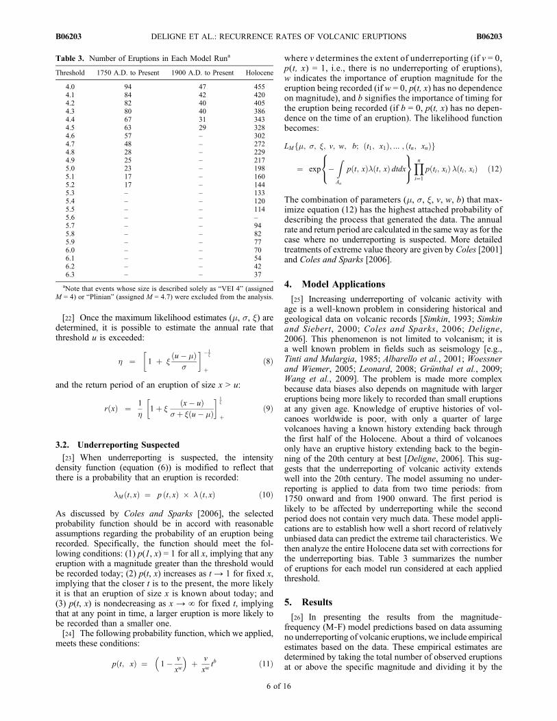
[25] Increasing underreporting of volcanic activity withage is a well‐known problem in considering historical andgeological data on volcanic records [Simkin, 1993; Simkinand Siebert, 2000; Coles and Sparks, 2006; Deligne,2006]. This phenomenon is not limited to volcanism; it isa well known problem in fields such as seismology [e.g.,Tinti and Mulargia, 1985; Albarello et al., 2001; Woessnerand Wiemer, 2005; Leonard, 2008; Grünthal et al., 2009;Wang et al., 2009]. The problem is made more complexbecause data biases also depends on magnitude with largereruptions being more likely to recorded than small eruptionsat any given age. Knowledge of eruptive histories of vol-canoes worldwide is poor, with only a quarter of largevolcanoes having a known history extending back throughthe first half of the Holocene. About a third of volcanoesonly have an eruptive history extending back to the begin-ning of the 20th century at best [Deligne, 2006]. This sug-gests that the underreporting of volcanic activity extendswell into the 20th century. The model assuming no under-reporting is applied to data from two time periods: from1750 onward and from 1900 onward. The first period islikely to be affected by underreporting while the secondperiod does not contain very much data. These model appli-cations are to establish how well a short record of relativelyunbiased data can predict the extreme tail characteristics. Wethen analyze the entire Holocene data set with corrections forthe underreporting bias. Table 3 summarizes the numberof eruptions for each model run considered at each appliedthreshold.

5. Results

[26] In presenting the results from the magnitude‐frequency (M‐F) model predictions based on data assumingno underreporting of volcanic eruptions, we include empiricalestimates based on the data. These empirical estimates aredetermined by taking the total number of observed eruptionsat or above the specific magnitude and dividing it by the

Table 3. Number of Eruptions in Each Model Runa

Threshold 1750 A.D. to Present 1900 A.D. to Present Holocene

4.0 94 47 4554.1 84 42 4204.2 82 40 4054.3 80 40 3864.4 67 31 3434.5 63 29 3284.6 57 – 3024.7 48 – 2724.8 28 – 2294.9 25 – 2175.0 23 – 1985.1 17 – 1605.2 17 – 1445.3 – – 1335.4 – – 1205.5 – – 1145.6 – – –5.7 – – 945.8 – – 825.9 – – 776.0 – – 706.1 – – 546.2 – – 426.3 – – 37

aNote that events whose size is described solely as “VEI 4” (assignedM = 4) or “Plinian” (assigned M = 4.7) were excluded from the analysis.


6 of 16

total time being considered. We stress that the models predictbehavior over time, so while the return levels of smaller(magnitude 5.0–5.5 eruptions) are sufficiently small such thatwithin the 259 or 109 years from which the data come, thenumber of eruptions divided by the time period studied reflectthe return periods, the return rates of the large eruptions donot. For instance, while the 1815 Tambora eruption (M = 6.9)happened during the time interval from 1750 to the present,and thus the empirical data indicates that oneM = 6.9 eruptionhappened in 259 years, the model, predicting behavior overtime, suggests a much longer return period than 259 years forsuch an eruption. We estimate upper and lower bounds forthe M‐F curves by calculating uncertainties at the 95%confidence interval.[27] In considering the results of our analysis we draw

attention to physical and geological constraints on values ofx. If x ≥ 0, the model predicts that there is no upper limit tothe size of an eruption, implying that an eruption could eruptmore than the mass of the earth. However, there is a physicalupper magnitude limit to explosive volcanic eruptions as aconsequence of the mechanisms of magma generation. Largebodies of silicic magma are generated by intracrustal igneousprocesses [Smith, 1979; Hildreth, 1981]. The volume ofmagma that can accumulate in a magma chamber is limitedby parameters such as crustal thickness, crustal strength,and magma supply rates [Jellinek and DePaolo, 2003]. Ourmodel takes none of these into consideration; rather than

modeling the details of the process to predict system limita-tions, we are using results of the process to predict the overallbehavior and limitations of the system. The data compilationof Mason et al. [2004b] on the largest explosive eruptionsindicates that there have been at least 42 magnitude 8 orgreater eruptions over the last 36 Myr, the largest of which isthe Fish Canyon Tuff eruption with M = 9.1–9.2 [Lipman etal., 1997; Bachmann et al., 2000]. These observations indi-cate that the upper bound for global volcanismmagnitude is atleast 9.2. While an unbounded solution is physically impos-sible, such a result could indicate that the data do not supportany particular value for the upper limit. If the maximumlikelihood estimate has x ≥ 0, making the high end resultscertainly invalid, one should note that the data support thismodel with x ≥ 0 as the best fit model, so it is the model to usefor other result interpretations, such as return periods forsmaller eruptions still within the end tail of the distribution.

5.1. Eruptions From 1750 to Present

[28] Figure 4 shows the data in the 1750 A.D. onwardperiod. Figure 5 shows the parameters (m, s, x) obtained atdifferent thresholds, with error bars indicating the 95%confidence interval. The precision, as quantified by the 95%confidence interval, greatly decreases (i.e., the confidenceinterval increases) for both m (location) and s (scale) atthreshold u = 4.7 and again at u = 5.0 (Figures 5a and 5b).While the model applied is more relevant at higher thresh-

Figure 4. Distribution of eruptions in compiled database (see auxiliary material) in the period from1750 A.D. to the present. The legend is as described in Figure 3.


7 of 16

olds, the errors associated with thresholds u = 5.0–5.2 aretoo large for any meaningful conclusions to be drawn. Wetherefore chose the threshold u = 4.9 as the optimum foranalysis and compared these with analyses with a thresholdu = 4.0, where all data are used. For two thresholds (u = 4.5and 4.6), the maximum likelihood value of x is greater thanzero, predicting no upper limit to the size of volcaniceruptions (Figure 5c). For six other thresholds the 95%confidence interval for x includes values equal to or greaterthan zero.[29] Figure 6 shows the return periods and predicted

magnitude limit for thresholds u = 4.0 (Figure 6a) and 4.9(Figure 6b) with calculations of upper and lower bounds ofuncertainty along with empirical data. For relatively lowmagnitude eruptions in the range M = 5.0 to 6.1, boththreshold models give M‐F curves that match the empiricaldata relatively well. The agreement is better for u = 4.9 thanfor u = 4.0. This demonstrates the principle that adding moredata from smaller eruptions (i.e., lowering the threshold)introduces more bias. Small eruptions are both unrepresen-tative of the tail and may also have a more pronouncedunderreporting problem then large eruptions. AboveM = 6.1the empirical data and the curves depart with the curvesgiving longer return periods than the empirical data. Aspreviously discussed, this is because the model predictsbehavior over time, while the empirical data simply reportshow many eruptions of or greater than a given magnitudehappened in the last 256 years. Thus, while there happenedto be an M = 6.9 eruption in the last 259 years (Tambora,1815), the model predicts that the long‐term average returnlevel for such an eruption is every 781 years (for u = 4.9).Table 4 lists the values for m, s, and x obtained for u = 4.0and 4.9, in addition to the values obtained for the analysisfor eruptions from 1900 A.D. to the present.[30] The models at thresholds u = 4.0 and 4.9 predict that

the largest possible explosive eruption magnitudes are 7.5 ±1.2 and 7.4 ± 1.8, respectively, with the error corresponding

to the 95% confidence interval. These two predicted mag-nitude limits are very similar, although when error is con-sidered the result obtained at u = 4.9 is close to containingthe largest known eruption of M = 9.2. We note that theincrease in error between u = 4.0 and 4.9 is due to thesparsity of data at the higher threshold (only 25 eruptions areconsidered at u = 4.9; see Table 3). It appears that while theperiod from 1750 A.D. to the present is sufficient for pro-ducing a return period model for thresholds below M ∼ 6, itis insufficient to characterize the M‐F relationship for largermagnitudes.[31] These results differ from those of Coles and Sparks

[2006] for their application of the same model to the por-tion of the Hayakawa catalog from 1600 A.D. to the present.Quite similar parameters were determined for model appli-cation at a threshold u = 4.0, although at higher thresholdsresults are less similar. Additionally, none of their values forx exceeded zero. The main differences between the dataused are that the Hayakawa catalog includes large effusiveeruptions, whereas our study only relates to explosiveeruptions, and that they assumed that there was no under-reporting from 1600 A.D. onward, which is suspect.

5.2. Eruptions From 1900 to the Present

[32] The same procedures have been applied to the dataset for the period since 1900 A.D. The advantage of thisperiod is that underreporting should not be a major problemfor large explosive eruptions, but the disadvantage is that theperiod is unlikely to sample the larger magnitude events wellor at all. The optimum choice of u = 4.5 was chosen andcompared with the analysis with u = 4.0. The maximumlikelihood M‐F curves (Figure 7) predict a limit for eruptionsize that is far too low considering the geologic record.Agreement between the analysis and the empirical data isgood up to aboutM = 5.7 for both thresholds. Taken togetherthese results suggest that the period is too short to be repre-sentative and to characterize the extreme tails.

Figure 5. Parameters obtained from application of extreme value statistics to the 1750 A.D. to presentperiod. The model assumes no underreporting of volcanic eruptions. For data where there are no obviouserror bars, the 95% confidence interval is too tight for the bars to appear. (a) Results for m, the locationparameter. (b) Results for s, the scale parameter. (c) Results for x, the rate of decay of the tail parameter.The dashed line shows where x = 0. At or above this line, the model predicts there is no upper limit to thesize of a volcanic eruption.


8 of 16

5.3. Analysis of Holocene Data

[33] Figure 3 shows the Holocene data for magnitudeversus age. Uncertainties vary greatly within the data set.Age uncertainties depend on geochronological methods andrange from precise historical fixes or precise tree ring cor-relations to scattered 14C ages with both corrected and uncor-rected results being reported. Typical age error estimates fornonhistorical age determination methods are ±250 years.

Magnitude error estimates are on the order of ±0.2. Error barsare not shown both for clarity, and also because in many casesthey are not reported. In our analysis we assume that theuncertainties are nonsystematic and will not affect the overallstatistical outcomes.[34] Underreporting is evident from visual inspection with

the density of data points decreasing back in time. The changein data density is more pronounced for smaller events than for

Figure 6. Return periods calculated at thresholds (a) u = 4.0 and (b) u = 4.9 from model application toeruptions in the 1750 A.D. to present period (solid line), with 95% confidence interval indicated by thedashed lines. The solid red line indicates the predicted magnitude limit, with the 95% confidence intervalindicated by the red dotted lines. The range of possible magnitudes for the Fish Canyon Tuff, the largestknown explosive eruption, is shown by the blue bar. Solid diamonds are the return periods empiricallycalculated from the data. This is done by dividing the total number of years of observations (259 years)by the number of eruptions at or above a given magnitude in that time.

Table 4. Model Parameters Obtained Using the 1750 A.D. to Present and 1900 A.D. to Present Data Setsa

Data Set u Threshold m Location s Scale x Shape Limit

1750 A.D. to present 4.0 2.62 ± 0.56 1.47 ± 0.62 −0.30 ± 0.16 7.51 ± 1.194.9 1.16 ± 4.68 2.38 ± 4.06 −0.38 ± 0.47 7.38 ± 1.77

1900 A.D. to present 4.0 2.76 ± 0.84 1.68 ± 1.12 −0.40 ± 0.30 6.94 ± 1.194.5 3.08 ± 1.59 1.27 ± 1.81 −0.29 ± 0.57 7.47 ± 4.06

aAssuming no underreporting of eruptions. Errors reported at the 95% confidence level.


9 of 16

larger events, reflecting the increased probability of recordinglarge eruptions. The plot includes data on Plinian eruptionsfor which there are no magnitude data but which are inter-preted as M > 4. These data have been assigned an arbitrarymagnitude of 4.7 and are excluded from the statistical anal-ysis. Additionally, data with an assigned VEI = 4 which werearbitrarily assigned a tephra volume of 0.1 km3 are likewiseexcluded from analysis.[35] We have estimated the parameters (m, s, x, v, w, b)

obtained at different thresholds, where the last three para-meters are those of the probability function (Figure 8). Theerror bars indicate the 95% confidence interval. The value ofx is below zero all thresholds (Figure 8c). For parametersthat describe underreporting we observe a modest effect ofmagnitude (Figure 8e) and a large effect of time (Figure 8f)reflected in large values of b for all thresholds. We chooseu = 5.5 as the preferred threshold that avoids the influenceof small magnitude eruptions to estimate the tail for the M‐Fcurve for extreme events. In addition, u = 5.5 is the highest

threshold with reasonable error that includes all the higherthresholds within the uncertainty limits.[36] Figure 9 shows the calculated probability of a M ≥ 6

eruption being recorded from the parameters obtained atthresholds u = 4.0 and 5.5. At the preferred threshold (u =5.5), the curves indicate that underreporting increases mark-edly between the present and 2000 years ago with a priorconstant value of about 20% for M ≥ 6 (Figure 9b). Theseresults give the probability that an eruption would be recordedwere it to have occurred during the reporting period. Colesand Sparks [2006] obtained similar probability functions intheir study of eruptions from the last 2000 years. Theirprobability function differs in that the sharp increase inprobability started around 1200 A.D. (as opposed to around1 A.D.). However, the initial probabilities for magnitude 6.0are almost identical to our results.[37] Figure 10 shows the return periods for thresholds u =

4.0 and 5.5. For this much longer time period the upperlimits are well below the expected value of aboutM = 9.2. In

Figure 7. Return periods calculated at thresholds (a) u = 4.0 and (b) u = 4.5 from model application toeruptions in the 1900 A.D. to present period (solid line), with 95% confidence interval indicated by thedashed lines. The solid red line indicates the predicted magnitude limit with the 95% confidence intervalindicated by the red dotted lines (note that for u = 4.5 the error is off the range of this plot; see Table 4).The range of possible magnitudes for the Fish Canyon Tuff, the largest known explosive eruption, isshown by the blue bar. Solid diamonds are the return periods empirically calculated from the data. This isdone by dividing the total number of years of observations (109 years) by the number of eruptions at orabove a given magnitude in that time.


10 of 16

this case the lower threshold (u = 4.0) gives a closer valueM = 8.3 ± 1.0 to the expected upper limit than the higherthreshold (u = 5.5) with a value of M = 7.6 ± 0.4; errorcorresponds to the 95% confidence interval. Overall, theconfidence intervals obtained are much tighter than thoseobtained for the analysis where no underreporting of erup-tions is suspected, which is not surprising as there are muchmore data and a much longer time period has been consid-ered. Table 5 lists the values for the parameters and pre-dicted upper limit obtained for u = 4.0 and 5.5.[38] As choice of threshold dictates the resulting return

period function and predicted magnitude limit, we includeFigure 11, which shows the predictedmagnitude limit obtainedat each threshold. Error bars indicate the 95% confidenceinterval. Six thresholds have a predicted magnitude limitgreater than M = 9.2; these six predictions also have thegreatest errors of any of the predicted limits obtained. Of theseventeen thresholds whose predicted magnitude limit is less

thanM = 9.2, the majority (ten) do not containM = 9.2 withintheir error bars.

6. Discussion

[39] The analysis of the Holocene data set on globalexplosive eruptions provides a statistically rigorous approachto assessing the return periods of large magnitude explosivevolcanic eruptions. However, it is important to acknowledgethat the model can only make predictions on the system thatthe data samples. Thus, if the data fail to sample a certainprocess, the model predictions will not apply to this process.Several issues arise from the results of the study that limit theability to constrain accurately the magnitude frequencyrelationship of very largemagnitude eruptions for which thereis little or no data during the Holocene, either as a conse-quence of such eruptions not having occurred over this timeperiod or having occurred but not yet being recorded by

Figure 8. Parameters obtained from application of extreme value statistics to the compiled database oflarge explosive Holocene eruptions. The model assumes underreporting of volcanic eruptions. Computa-tion problems excluded the determination of parameters at thresholds u = 5.6. For data where there are noobvious error bars, the 95% confidence interval is too tight for the bars to appear. (a) Results for m, thelocation parameter. (b) Results for s, the scale parameter. (c) Results for x, the rate of decay of the tailparameter. The dashed line shows where x = 0. At or above this line, the model predicts there is no upperlimit to the size of a volcanic eruption. (d) Results for v, the extent of underreporting parameter. (e) Re-sults for w, the magnitude parameter. (f) Results for b, the timing parameter.


11 of 16

geological studies or because the processes involved are notcaptured by the modeling of smaller magnitude eruptions andthe extrapolation of the results. Here we discuss these issuesand propose a current state of knowledge on return periodsand assess the uncertainties in these estimates.[40] The study quantifies the degree of underreporting

back in time. Starting about 2000 years ago there is a rapidincrease in the probability that an event is recorded, whichreflects the spread of historical written records and advancesin science. Prior to 2000 years ago underreporting is sta-tistically constant. This result reflects the fact that the datafor volcanism prior to 2000 years are largely obtained bygeological studies and if a study is done, the Holocenerecord of tephra from large magnitude vents for a particularvolcano is fairly complete. If there is a decrease in preser-vation potential between the start of the Holocene and2000 years ago, then our results do not detect this effect. Forour preferred threshold value the underreporting is estimatedat approximately 80% for M ≥ 6. This predicts that if amagnitude 6.0 or greater eruption (approximately 1991Mt. Pinatubo size eruption or above) occurred prior to 1 A.D.,there is only a one in five chance that we know about it today.As previously mentioned, the probability of a Holoceneeruption happening prior to 1 A.D. and the scientific com-munity not knowing about it today is the probability of it

being recorded times the probability of it happening duringthe length of time of interest (in this case, 10,000 years).These results concerning the state of knowledge are similar tothose obtained by an independent method assessing how farback volcanic histories extend from an analysis of a globaldatabase of volcanoes [Deligne, 2006], which found thatonly a quarter of the world’s volcanoes with potential forexplosive volcanism have records extending back earlier than3000 BC. Underreporting is also dependent on magnitudewith recording probability increasing with magnitude.[41] The choice of a threshold is important in character-

izing the tail of the distribution and is a tradeoff betweendata quantity and data relevance. A low threshold increasesthe data quantity, decreasing apparent confidence intervals,but biases the analysis with data from relatively low mag-nitude events, which may be unrepresentative of the naturalprocesses that govern the tail. A high threshold may bebetter at characterizing the tail but the uncertainties increasemarkedly due to the reduction in data. Comparison of theresults for different thresholds indicates that these effects areimportant in the explosive volcanism data set. Thus wepropose that the best representation of the M‐F relationshipof the tail is for u = 5.5 for the Holocene data set. Even withthis choice of threshold that excludes the smaller events theresults suggest that the extreme region of the tail is not yet

Figure 9. Probability function that an eruption of magnitude 6.0 is known about today, as determined atthresholds (a) u = 4.0 and (b) u = 5.5.


12 of 16

captured in the model. The maximum likelihood result withu = 5.5 gives an upper limit for an extreme event of onlyM = 7.6 with an upper bound slight above M = 8. How-ever, the geological record shows that M > 8 occur, albeitvery rarely, and the largest known eruption has M = 9.2;this is probably close to the true maximum [Mason et al.,2004b]. Figure 11 shows that most thresholds with apredicted magnitude limit containing reasonable error donot contain M = 9.2 within their 95% confidence intervals;the predicted magnitude limit is in such case smaller. Fromthis is clear that the model based on Holocene data doesnot capture the very extreme tail.[42] The failure to capture the extreme parts of the tail can

be attributed to two possible causes. First the largest mag-

nitude eruption in the Holocene data set is M = 7.4.Extrapolation of best fit models well beyond the largestevent that has been analyzed is problematic if the extremeevents do not follow the same frequency distribution as thesmaller events in the data set. This is not just an issue of theuncertainties increasing with increased extrapolation sinceour analysis includes estimates of uncertainty and the upperbounds fall well short of the M > 8 events. This observationsuggests the second possibility, that different physicalmechanisms may be responsible between large and verylarge magnitude events.[43] Such different mechanisms are known in other sys-

tems. For example, Sparks and Aspinall [2004] analyzed thestatistical distribution of durations of 150 historic lava dome

Figure 10. Return periods calculated at thresholds (a) u = 4.0 and (b) u = 5.5 from model application toHolocene eruptions (solid line), with 95% confidence interval indicated by the dashed lines. The solid redline indicates the predicted magnitude limit, with the 95% confidence interval indicated by the red dottedlines. The range of possible magnitudes for the Fish Canyon Tuff, the largest known explosive eruption, isshown by the blue bar.

Table 5. Model Parameters Obtained Using the Holocene Data Seta

u Threshold m Location s Scale x Shape v Extent w Magnitude b Time Limit

4.0 7.70 ± 0.48 0.14 ± 0.08 −0.25 ± 0.09 1.30 ± 0.21 0.21 ± 0.11 16.03 ± 4.91 8.27 ± 0.995.5 7.39 ± 0.22 0.08 ± 0.07 −0.39 ± 0.22 1.09 ± 3.23 0.18 ± 1.65 11.76 ± 10.41 7.59 ± 0.43

aAssuming underreporting of eruptions. These value were obtained by rescaling time in the Holocene from 0 to 1; thus, any estimates for return periodsmust by multiplied by 10,009 (i.e., time between 8000 B.C. and 2009 A.D.) to obtain return period in years. Errors reported at the 95% confidence level.


13 of 16

eruptions. The M‐F curve for duration changed at about5 years duration with a long‐duration tail, which is quitedifferent to the M‐F curve for the majority of the data. Thus,the processes involved for short‐duration (less than 5 years)lava dome eruption appear to be different from processesinvolved in long‐duration events. In this case, Sparks andAspinall [2004] suggested that dome eruptions lastingmore than 5 years form thermally mature conduits whichallow prolonged magma flow and eruption. Irrespective ofthe cause the data support contrasted physical mechanismsbetween long‐ and short‐duration dome eruptions.

[44] In the case of explosive volcanism we propose thatthere is a change in the physical mechanism between largeand very large magnitude explosive eruptions. A clue to thenature of the change is that caldera formation becomes amajor feature of explosive eruptions at about M ∼ 7. The sixHolocene eruptions that exceed M ∼ 6.9 all formed calderas.Additionally, the data set of Mason et al. [2004b] forM > 8 events support a different M‐F relationship for caldera‐forming eruptions. Many of the eruptions in our data setare for Plinian style eruptions from stratovolcanoes or cen-tral vents and were not accompanied by caldera formation.

Figure 11. Predicted magnitude limit of all thresholds with calculated Holocene parameters, with errorbars showing the 95% confidence interval. For u = 4.6, the predicted magnitude limit is M = 22.6, and foru = 4.3, 4.5, 4.6, 4.7, and 6.0, the full range of the 95% confidence interval is greater than the range of theplot. The range of possible magnitudes for the Fish Canyon Tuff, the largest known explosive eruption, isshown by the blue bar.

Table 6. Predicted Return Levels for Eruptions of Different Magnitudes According to Different Model Runs

Eruption Magnitude Eruption Example

Predicted Return Levels (years)

Holocene 1750–Present 1900–Present

u = 4.0 u = 5.5 u = 4.0 u = 4.9 u = 4.0 u = 4.5

4.5 Avachinsky, 1945 4.4 – 5.0 – 3.8 3.95.0 Somma‐Vesuvius, 1631 7.9 – 9.2 12 6.7 7.35.5 Shiveluch, 1964 15 24 19 23 14 166.0 Quizapu, 1932 35 49 50 51 41 446.5 Krakatau, 1883 96 129 191 163 268 1847.0 Kurile Lake, KO eruption 370 626 1850 1428 – 2249


14 of 16

The study of Jellinek and DePaolo [2003] provides aplausible explanation for a change of mechanism betweensmaller magnitude Plinian eruptions and larger magnitudecaldera‐forming eruptions. They propose that a change inbehavior occurs when magma chambers reach a critical size.Below the critical size the chamber cannot sustain largepressures and conditions are repeatedly reached when dykescan propagate and eruptions can take place. In such systemsthe chamber erupts relatively frequently and does not growto a size where very large magnitude eruptions are possible.Once the size threshold is crossed, however, the conditionsallow the chamber to grow by progressive magma accu-mulation and prevent dyke propagation. The magmaticsystem can then grow to a large volume and other triggeringmechanisms become important, such as failure of the crustallid to the chamber [Jellinek and DePaolo, 2003]. As in thecase of lava dome durations, the two styles of magma chamberevolution and associated volcanismmight be expected to givedifferent M‐F relationships.[45] If our interpretation of different mechanisms is cor-

rect then extrapolation of the curves to large magnitude isnot justified. A major objective of future research should beto gather data for M > 7 explosive eruptions over a longertime period than the Holocene. There effectively is a datagap between the study of Mason et al. [2004b] for M >8 explosive eruptions and our study which likely covers tooshort a period to sample eruptions in the M = 7 to 8 range.[46] We are confident that the curves up to M ∼ 6.5 are

robust representations of the global M‐F relationships. InTable 6 we tabulated the predicted return period for erup-tions between magnitude 4.5 and 7 in intervals of 0.5. ForM ≥ 7 the uncertainties remain large and will need moreextensive time period data sets as well as investigation ofthe underlying mechanisms.

7. Summary and Conclusions

[47] We compiled a database of large explosive Holoceneeruptions, with the aim of including every known eruptionof magnitude 4 or greater. A total of 576 eruptions from 227volcanoes were included. Extreme value theory statisticswas applied to the resulting database. A model assuming nounderreporting of volcanic eruptions was applied to two datasets, one of eruptions from 1750 A.D. to the present anda second from 1900 A.D. to the present. A model takingunderreporting into consideration was applied to the entireHolocene database. Results in all cases predict eruption sizelimits smaller than most supereruptions and considerablythan the largest known volcanic eruption, the Fish CanyonTuff. Additionally, results from the Holocene analysis implyconsiderable underreporting of volcanic eruptions prior to1 A.D., predicting that a magnitude 6 eruption only has a 20%chance of being recorded. We suggest that the models predicta smaller magnitude eruption size limit than the geologicrecord indicates due to sampling biases. It is likely that thedata only sampled the high end of “ordinary” eruptions andthat the mechanisms behind “supereruptions” are different.Our results hence predict the upper limit and recurrence ratesfor large Plinian‐type eruptions but do not make predictionson size or recurrence rates of caldera‐forming eruptions, thehigh end of which are “supereruptions.”

[48] Acknowledgments. This project is a product of the VOGRIPAproject, supported by Munich Re and the European Research Council. VO-GRIPA is part of the Global Risk Identification Programme (GRIP). R.S.J.S.acknowledges support of a Royal Society Wolfson Merit Award and aEuropean Research Council Advanced Grant. We thank Matt Watson andNick Tanushev for support to N.I.D. with preparation of the data and com-puting. This work reflects part of the work N.I.D. did for her Masters thesisat the University of Bristol. This manuscript was improved by commentsfrom Warner Marzocchi, Patrick Taylor, and two anonymous reviewers.

ReferencesAlbarello, D., R. Camassi, and A. Rebez (2001), Detection of space andtime heterogeneity in the completeness of a seismic catalog by a statisti-cal approach: An application to the Italian area, Bull. Seismol. Soc. Am.,91(6), 1694–1703, doi:10.1785/0120000058.

Ammann, C. M., and P. Naveau (2003), Statistical analysis of tropicalexplosive volcanism occurrences over the last 6 centuries, Geophys.Res. Lett., 30(5), 1210, doi:10.1029/2002GL016388.

Bachmann, O., M. A. Dungan, and P. W. Lipman (2000), Voluminouslava‐like precursor to a major ash‐flow tuff: Low‐column pyroclasticeruption of the Pagosa Peak Dacite, San Juan volcanic field, Colorado,J. Volcanol. Geotherm. Res., 98, 153–171, doi:10.1016/S0377-0273(99)00185-7.

Caniaux, G. (2005), Statistical analysis of the volcanic eruption frequencyin the Azores islands: A contribution to risk assessment, Bull. Soc. Geol.Fr., 176, 107–120, doi:10.2113/176.1.107.

Coles, S. G. (2001), An Introduction to Statistical Modeling of ExtremeValues, 208 pp., Springer, London.

Coles, S. G., and R. S. J. Sparks (2006), Extreme value methods for mod-elling historical series of large volcanic magnitudes, in Statistics in Vol-canology, Spec. Publ. of the Int. Assoc. of Volcanol. and Chem. of theEarth’s Inter., vol. 1, edited by H. M. Mader et al., pp. 47–56, Geol.Soc., London.

Connor, C. B., R. S. J. Sparks, R. M. Mason, C. Bonadonna, and S. R.Young (2003), Exploring links between physical and probabilistic mod-els of volcanic eruptions: The Soufrière Hills Volcano, Montserrat,Geophys. Res. Lett., 30(13), 1701, doi:10.1029/2003GL017384.

Deligne, N. I. (2006) Large explosive volcanic eruptions: Completeness ofthe Holocene record and application of extreme value statistics, M.Sc.thesis, 69 pp., Univ. of Bristol, Bristol, U. K., 11 Jan.

Gan, Z. J., and C. C. Tung (1983), Extreme value distribution of earthquakemagnitude, Phys. Earth Planet. Inter., 32, 325–330, doi:10.1016/0031-9201(83)90032-8.

Grünthal, G., R. Wahlström, and D. Stromeyer (2009), The unified cata-logue of earthquakes in central, northern, and northwestern Europe(CENEC)—Updated and expanded to the last millennium, J. Seismol.,13, 517–541, doi:10.1007/s10950-008-9144-9.

Hildreth, W. (1981), Gradients in silicic magma chambers: Implications forlithospheric magmatism, J. Geophys. Res., 89, 8441–8462.

Huppert, H. E., and R. S. J. Sparks (2006), Extreme natural hazards: Pop-ulation growth, globalization and environmental change, Philos. TransR. Soc. A, 364, 1875–1888, doi:10.1098/rsta.2006.1803.

Jellinek, A. M., and D. J. DePaolo (2003), A model of the origin of largesilicic magma chambers: Precursors of caldera‐forming eruptions, Bull.Volcanol., 65, 363–381, doi:10.1007/s00445-003-0277-y.

Jones, G., D. K. Chester, and F. Shooshtarian (1999), Statistical analysis ofthe frequency of eruptions at Furnas Volcano, Sao Miguel, Azores,J. Volcanol. Geotherm. Res., 92, 31–38, doi:10.1016/S0377-0273(99)00065-7.

Kim, S. G. (1983), On the estimation of parameters in the statistical predic-tion of earthquakes, J. Phys. Earth, 31, 251–264.

Lavenda, B. H., and E. Cipollone (2000), Extreme value statistics and ther-modynamics of earthquakes: Aftershock sequence, Ann. Geofis., 43,967–982.

Leonard, M. (2008), One hundred years of earthquake recording in Austra-lia, Bull. Seismol. Soc. Am., 98, 1458–1470, doi:10.1785/0120050193.

Lipman, P., M. Dungan, and O. Bachmann (1997), Comagmatic grano-phyric granite in the Fish Canyon Tuff, Colorado: Implications formagma‐chamber processes during a large ash‐flow eruption, Geology,25, 915–918, doi:10.1130/0091-7613(1997)025<0915:CGGITF>2.3.CO;2.

Marzocchi, W., and L. Zaccarelli (2006), A quantitative model for the time‐size distribution of eruptions, J. Geophys. Res., 111, B04204,doi:10.1029/2005JB003709.

Mason, B. G., D. M. Pyle, W. B. Dade, and T. Jupp (2004a), Seasonality ofvolcanic eruptions, J. Geophys. Res., 109, B04206, doi:10.1029/2002JB002293.


15 of 16

Mason, B. G., D. M. Pyle, and C. Oppenheimer (2004b), The size and fre-quency of the largest explosive eruptions, Bull. Volcanol., 66, 735–748,doi:10.1007/s00445-004-0355-9.

Naveau, P., and C. M. Ammann (2005), Statistical distribution of ice coresulfate from climatically relevant volcanic eruptions, Geophys. Res. Lett.,32, L05711, doi:10.1029/2004GL021732.

Newhall, C. G., and S. Self (1982), The volcanic explosivity index (VEI):An estimate of explosive magnitude for historical volcanism, J. Geophys.Res., 87, 1231–1238, doi:10.1029/JC087iC02p01231.

Pisarenko, V. F., and D. Sornette (2003), Characterization of the frequencyof extreme earthquake events by the Generalized Pareto Distribution,Pure Appl. Geophys., 160, 2343–2364, doi:10.1007/s00024-003-2397-x.

Pyle, D. M. (2000), Sizes of volcanic eruptions, in Encyclopedia of Volca-noes, edited by H. Sigurdsson, pp. 263–269, Academic, San Diego, Calif.

Siebert, L., and T. Simkin (2002), Volcanoes of the World: An IllustratedCatalog of Holocene Volcanoes and Their Eruptions, Digital Inf. Ser.,GVP‐3, Global Volcan. Program, Smithson. Inst., Washington, D. C.(Available at http://www.volcano.si.edu/world/)

Simkin, T. (1993), Terrestrial volcanism in space and time, Annu.Rev. Earth Planet . Sci . , 21 , 427–452, doi:10.1146/annurev.ea.21.050193.002235.

Simkin, T., and L. Siebert (2000), Earth’s volcanoes and eruptions:An overview, in Encyclopedia of Volcanoes, edited by H. Sigurdsson,pp. 249–262, Academic, San Diego, Calif.

Smith, R. L. (1979), Ash‐flow magmatism, Spec. Pap. Geol. Soc. Am., 180,5–27.

Sparks, R. S. J., and W. P. Aspinall (2004), Volcanic activity: Frontiers andchallenges in forecasting, prediction and risk assessment, in The State ofthe Planet: Frontiers and Challenges in Geophysics, Geophys. Monogr.Ser., vol. 150, edited by R. S. J. Sparks and C. J. Hawkesworth, pp. 359–373, AGU, Washington, D. C.

Tinti, S., and F. Mulargia (1985), An improved method for the analysis ofthe completeness of a seismic catalogue, Lett. Nuovo Cimento Soc. Ital.Fis., 42, 21–27, doi:10.1007/BF02739471.

Wang, Q., D. D. Jackson, and Y. Y. Kagan (2009), California earthquakes,1800–2007: A unified catalog with moment magnitudes, uncertainties,and focal mechanisms, Seismol. Res. Lett., 80, 446–457, doi:10.1785/gssrl.80.3.446.

Woessner, J., and S. Wiemer (2005), Assessing the quality of earthquakecatalogues: Estimating the magnitude of completeness and its uncer-tainty, Bull. Seismol. Soc. Am., 95, 684–698, doi:10.1785/0120040007.

S. G. Coles, Smartodds, Unit 612, Highgate Studios, 53‐79 HighgateRd., London NW5 1TL, UK.N. I. Deligne, Department of Geological Sciences, 1272 University of

Oregon, Eugene, OR 97403‐1272, USA. ([email protected])R. S. J. Sparks, Department of Earth Sciences, University of Bristol,

Wills Memorial Building, Queen’s Road, Bristol BS8 1RJ, UK.


16 of 16

recurrence rates of large explosive volcanic eruptions€¦ · recurrence rates of large explosive...

Documents