recursive 3-d motion estimation from a monocular [4, …raghuram/enee731/sfm/00055557.pdf ·...

I . INTRODUCTION

Recursive 3-D Motion Estimation from a Monocular Image Sequence

‘E J. BROIDA Hughes Aircraft Co.

S. CHANDRASHEKHAR, Student, IEEE

R. CHELLAPPA, Senior Member, IEEE Signal and Image Processing Institute

The problem considered here involves the design and application of a recursive algorithm to a sequence of images of a moving object to estimate both its structure and kinematics. The object is assumed to be rigid, and its motion is assumed to be “smooth” in the sense that it can be modeled by retaining an arbitrary number of terms in the appropriate Taylor series expansions. Translational rmtion involves a standard rectilinear model, while rotational rmtion is described with quaternions. Neglected terns of the Taylor series are modeled as process noise. A state-space d e l is constructed, incorporating both kinematic and structural states, and recursive techniques are used to estimate the state vector as a function of time.

consisting of Tied features on the object, the image plane coordinates of which have been extracted from successive images in the sequence. The measured data are the noisy image plane coordinates of this set (or of a subset of this set) of object match points, taken from each image in the sequence. High iniage plane noise levels (up to N 10 percent of the object image size) are allowed. The problem is formulated as a parameter estimation and tracking problem, which can use an arbitrarily large number of images in a sequence. The recursive estimation is done using an iterated extended Kalman filter (IEKF), initialized with the output of a batch algorithm run on the first few frames. Approximate Crad r -Rao lower bounds on the error covariance of the batch estimate are used as the initial state estimate error covariance of the IEKF. The performance of the recursive estimator is illustrated using both real and synthetic image sequences.

A set of object match points is assumed to be available,

Manuscript received April 10, 1989; revised November 4, 1989 and January 3, 1990.

IEEE Log No. 36730.

This work was partially supported by the Office of Naval Research under the grant “14-89-5-1598.

Authors’ addresses: T. J. Broida, Hughes Aircraft Co., Radar Systems Group, Los Angeles, CA 90009; S. Chandrashekhar and R. Chellappa, Signal and Image Processing Institute, Dep’t. of Electrical Engineering, University of Southern California, Los Angeles, CA 90089-0272.

0018-9251/90/0700-0639 $1.00 @ 1990 IEEE

Two fundamentally distinct approaches exist for obtaining measurement data for motion estimation. Optical flow methods represent motion in the image plane as sampled, continuous velocity fields [l-31. Work such as [4, 51 demonstrates the usefulness of this type of approach, in terms of the “low-level” problems of motion recognition and segmentation of scenes into their moving and stationary components, when the camera is itself moving.

Feature based methods rely on the recognition of the same set of correspondence points-points that arise from the same feature of the object-in two or more images. Then, various approaches can be taken towards estimation of object motion. The approach presented here is based on the use of discrete features.

A substantial amount of work has been devoted to methods for estimating object motion based on a short sequence of images. Many existing methods define object motion to be a single rigid body transformation that takes an object from its spatial position at the time of one image to its position at the time of a second image. This transformation can be represented by a single translational increment, followed or preceded by a rotational increment about a single axis. Since the time between images can be measured, the result is an approximation of translational and rotational velocities.

Much existing work begins by assuming that the problems of extracting feature points and establishing the required correspondences have been accomplished. Roach and Aggarwal [6] develop a system of nonlinear equations that relate the measured image plane coordinates, the ( x , y , z ) coordinates on the object, and the camera position parameters. Numerical techniques for solving the nonlinear equations are discussed, as well as methods for choosing good initial conditions and handling noise in the data.

Assuming that rotational increments are small, Tsai and Huang, in [7, 81, give an elegant analysis of the motion estimation problem that addresses both the computational and theoretical problems. In [7] it is shown that the eight “pure parameters” relating the spatial positions of the object match points in successive images are unique, given several constraints on the spatial relationships of the match points. Using a singular value decomposition of the “pure parameters” matrix, the conditions under which the motion parameter estimates are unique are discussed in [SI.

Fang and Huang [9] have implemented the approach, and present detailed experimental results. They report successful experiments in extracting features and establishing match point correspondence when the rotation and scale change between successive images is small.

geometry approach is made. This involves introducing a In [lo], a modification to the pure projective

IEEE TRANSACTIONS ON AEROSPACE AND ELECTRONIC SYSTEMS VOL. 26. NO. 4 JULY 1990 639

regularization term so as to find the feasible rotation with minimum magnitude. Experiments conducted for more (up to 30) match points show that for large numbers of points (more than about 20) the pure projective geometry method works as well as the regularization approach is not improved significantly by the use of more points. A n attempt to use more than two images in the sequence is also made, by averaging the results of each of the successive pairs. This is shown to give no significant improvement.

It is widely held that most existing schemes for motion estimation perform very poorly when the data (image coordinates of match points) are noisy [6, 9-11]. In [6, 7, 93 smoothing is achieved by using a larger number of match points in each image. This gives some improvement [9, 101, but as discussed in [12], using additional match points in each frame introduces additional unknown parameters, which limits the amount of new information that can be incorporated by this means. The alternative is to use a larger number of image frames. To use an arbitrary number of frames, the number of unknown model parameters should not be a function of the number of image frames used. The object motion model presented here has this property; models used in [6, 7, 9, 101 do not. The models used in [13, 141 are quite similar to those used in our research, but differ in certain ways: [13] assumes known structure, [14] uses specific models for different situations (e.g., number of feature points, number of image frames). In [15] an integrated spatio-temporal approach is developed, which can be tailored to specific applications such as automated land vehicle guidance. In [16] this rotational modeling is addressed by combining multiple solutions of the two-view problem using a local conservation of angular momentum (LCAM) model. However, the real image experiments reported there involve stereo imagery only.

The use of a larger number of images in the sequence allows significant smoothing to be achieved. In addition, the problem of forming parameter estimates in the presence of match point occlusion or temporary object occlusion can also be addressed in a natural manner, since the evolution of the model parameters with time is the basis of the general approach. Further, the recursive solution could be a starting point towards solving the problem of finding the same set of object match points in successive image frames, since match point locations and image coordinates can be extrapolated to the next image based on model parameter estimates.

for the motion of an object, the time-evolution of this motion, and the observation of the object, and to formulate the problem as one of recursive state estimation. Fig. 1 illustrates the basic models for motion, structure, and the observation of the object. First, the use of truncated Tiylor series

Our basic approach has been to develop models

/ yo obiect translation

match point 2

inertial coordinate system

Fig. 1. Conceptual illustration of object motion and imaging.

allows the incorporation of as many derivatives as desired in modeling motion, both translational and rotational. The choice of standard rectilinear states for translational motion results in linear time-evolution. However, rotational motion is more complex, and unavoidably nonlinear. Fortunately, the use of quaternions allows at least a closed form propagation in time of rotational motion with either constant velocity or constant precessional rate.

Next, an object-centered coordinate system is defined. Translation is that of the origin of this coordinate system, and rotation is about the origin of this system. Object feature points are constant in this coordinate system, since the object is assumed to be rigid. The camera-centered coordinate system is assumed to be inertial (nonaccelerating). The inertial (camera-centered) coordinates of an object feature point are just the inertial coordinates of the origin of the object-centered system added to the object-system coordinates of the feature point. These concepts are made precise in the next section. Using the central projection imaging model, the image of each point is then simply the ratio of its inertial x and y coordinates to its z coordinate, multiplied by the focal length of the imaging system.

Finally, based on N frames of data, with noisy image coordinates of M features in each frame, we form estimates of the unknown parameters (elements of the state vector) in the above models. The plant equation is based on the motion model, and indicates how the parameters to be estimated evolve in time.

640 IEEE TRANSACTIONS ON AEROSPACE AND ELECTRONIC SYSTEMS VOL. 2.6, NO. 4 JULY 1990

BROIDA, ET AL.: RECURSIVE 3-D MOTION ESTIMATION FROM A MONOCULAR IMAGE SEQUENCE 641

The measurement equation is based on the central projection model of image formation. The nonlinear nature of both equations precludes a simple Kalman filtering approach, and hence an approximate nonlinear filtering approach is used. An iterated extended Kalman filter (IEKF) [17] is designed for the problem, and its performance on real and synthetic images is studied. Experiments show that the IEKF performs very well when the initial guess supplied to it is obtained by running a batch estimation algorithm on the first few images in the sequence [18], and the approximate Cram&-Rao lower bounds [19] on the batch estimate are used as the error covariance of the initial guess.

Here, feature point correspondences are assumed to be available; a method for obtaining them is suggested in the Appendix, but it has not been implemented so far in our research. A similar method has been implemented by Dickmanns [20], who employs “constrained correlation” to obtain the match points.

is discussed in [18, 21-23]. In [21] a one-dimensional (1-D) image of a two-dimensional object (2-D) undergoing 2-D motion was examined, to explore the properties of central projection imaging and the viability of the object/motion modeling approach. Some knowledge of object structure was assumed, and a recursive solution method was used on simulated data. The favorable results presented there were extended to a 2-D image of a 3-D object, undergoing 3-D motion, and the various models were more fully developed-this research was reported in a workshop [18]. A recursive solution was applied to simulated imagery involving pure translation and unknown structure. In [22], rotational motion was included, and a batch approach was applied to synthetic data; the experiments involved known object structure. In [23], the general case of unknown structure and motion (both translational and rotational) was addressed, and a batch method was shown to be effective in two experiments involving real imagery. Here we deal with the more general case of motion involving both translation and rotation, assuming no knowledge about the structure of the object undergoing motion.

Previous work by Broida and Chellappa in this area

II. MODELS

The fundamental model of this paper is that the motion of the rigid object during the observation period is smooth enough so that it can be represented by a dynamic model of relatively low dimensionality. The constraint imposed on the motion is that some finite time derivative (say, the nth) of the variation in each kinematic attribute be constant. That is, a constant first derivative implies constant velocity, constant second derivative implies constant

acceleration, etc. Further, the model allows a different value of n for rotation and translation.

A. Imaging Model

A central projection imaging model is assumed, defined by

h : S H P (1)

is a spatial point coordinate,

p = ( X , Y ) T E P c R2 (3) is an image plane point coordinate. The space P is nominally a finite rectangle, corresponding to the image plane of a camera. Then,

Z Z (4) X Y X = f . - + + x ; Y = f . - + n y

map spatial coordinates to noisy image coordinates, where the camera focal length f is set to unity w.1.o.g. The terms n x and ny are the image plane noise components, discussed below. Thus, the measurement model for a single point s = ( x , ~ , z ) ~ is

p = (t) = ( X / z ) + (;;) = h[s] + n. ( 5 ) Y /z

The measured image coordinates of the match points are assumed to consist of the image coordinates of the true feature positions corrupted by additive independent zero mean Gaussian noise.

B. Object and Motion Model

An object-centered coordinate system is defined. The origin of this object-centered coordinate system is not observed, in general. Object structure is then defined as the coordinates of the object match points in the object-centered coordinate frame. These positions are constant in time due to the rigidity assumption. Object translational kinematics are defined to be the position and motion of the origin of the object-centered coordinate frame with respect to the camera-centered (inertial) coordinate frame. Object rotational lunematics are defined to be the object angular position and motion about the origin of the object-centered frame expressed in the inertial camera-centered coordinate system. Object structure and translational kinematics can only be known to within a global scale factor, unless absolute a priori data is available about the object and/or its translational kinematics. Object rotational kinematics are not subject to this scale factor. The scale factor comes about because, as can be seen from the mapping h defined in (5 ) , any constant multiple of all spatial coordinates ( x , ~ , z ) ~ results in the same image.

The following model results. Let si0 = (x ; ,~ ; ,z ; )~ be the object-centered coordinates of match point i. Let S R ( ~ ) = (xR(~),YR(~),zR(~))~ be the camera-centered (inertial) coordinates of the origin of the translating object reference frame (not observed directly). Let R(t) be the 3 x 3 coordinate transformation matrix that aligns the object coordinate axes with the camera coordinate axes, changing with time (rotating object). Let si(t) be the spatial, camera-centered coordinates of match point i at time t .

The object motion model is then given by

At time tk the image plane measurements of the match points are, from ( 5 ) ,

which can be written as

where i = 1,. . . , M for M object match points. This cannot be simplified further, because h is nonlinear.

C. Translational Motion Model

Since the spatial coordinates of the object-centered reference frame S R ( ~ ) can be written in terms of an arbitrary number of derivatives, a variety of modeling options are available. Assuming it can be accurately modeled by a constant nth derivative,

Thus, the translational motion during the observation period is modeled by a finite number (3n) of parameters, which are simply the nonzero derivatives at a single point in time.

D. Rotational Motion Model

Quaternions, described for example in [24-261, can be used to propagate the transformation matrix R(t) in time, with the rotation of the object coordinate frame represented by the object rotation rates about its (x ,y ,z) axes, wf = ( ~ , , w ~ , w , ) ~ . With this approach, the rotation matrix R(t) can be written in terms of the unit quaternion q(t) = (ql(t),q2(t), q3(t),q4(t))T as discussed in [24-261. Suppressing the time dependency,

R =

642 IEEE TRANSACTIONS ON AEROSPACE A N D ELECTRONIC SYSTEMS VOL. 26, NO. 4 JULY 1990

or, more briefly,

The unit quaternion q = (qt,qz,q3,q4)= is related to “standard” expressions of the angular relation between coordinate systems by the relation

(41, q 2 , q3, q4)T = (n 1 sin 6/2, n2 sin 6/2, n3 sin 6/2, cos 0/2)T

(11)

where (nl,n2,n3) is the axis of rotation, and 8 is the angle about the axis that aligns the coordinate axes of the rotating coordinate system with those of the reference system. It is termed a unit quaternion because 141 = 1. The quaternion q propagates in time according to the differential equation [25, 261

The solution to (12) when w is constant is simply

It also might be noted that the matrix 2iR/lwl is unitary, where i = a. As a result, the power series expansion for the matrix exponential can be reduced to P61

I 2 . COS(lUl(t - fo)/2)14 4- -Sln(lUl(t - f0)/2)0 ¶ ( t o )

Iw I

which can be further reduced by assuming that the coordinate systems are aligned at to = 0, so that q(0) = (O,O,O, l)T, and

However, this solution is valid only when w is constant. In general, the image of the match points at time tk can be written, from (€9,

The reason for resorting to quaternions is that the differential equation of (12) describing their time-propagation is much simpler than the analogous system for propagating Euler angles, even when higher derivatives are involved. In addition, the body rates w are more meaningful, intuitively, than are the Euler rates, since the latter are defined about nonorthogonal axes. As discussed in [27], motion involving constant precessional rate can also be expressed in closed form

with quaternions. In order to represent higher order rotational derivatives, w could be expanded in Taylor series as in (9), and the differential equation of (12) could be integrated numerically, with time-varying W. However, Cram&-Rao lower bound results [19] indicate that very large amounts of accurate data would be required for such higher order rotational motion.

Ill. FORMULATION FOR RECURSIVE SOLUTION

The use of a recursive procedure for parameter estimation is not viewed as an alternative to the batch procedure. Instead, an estimation “system” is envisioned, in which a batch method is applied to an initial set of data, that is used to initialize a recursive procedure. The recursive algorithm is then used to “track” the object and its motion. The value of this type of approach is that recursive methods usually require much less computation time for each new set of data (each new image, for example), they continually compute state estimates indexed to the current time, based on all past data, and can readily extrapolate the state estimates ahead in time to aid in preprocessing the next set of data.

Another aspect of recursive filtering, in this context, is that approximate filters are required, due to the nonlinear nature of both the plant and the measurement processes. On the one hand, this means that the state estimates are not sufficient statistics for the past data, as they are in the linear case, so there is an inefficiency in the use of data, with degradation of state estimates. On the other hand, if the models are only approximations to the true plant and measurement processes, then the “limited memory” of this type of recursion can be advantageous, since “small” deviations from the models are tolerated, and tracked, without the need for explicit modeling. Thus, if a constant velocity model is used for the object motion, but there is in reality some deviation from this model (trajectory perturbations, small random accelerations, small constant accelerations, etc.), then a recursive algorithm will track the actual object kinematics, and “forget” about data taken at earlier times. A batch method would give the best “straight-line” (constant velocity) estimate for all of the data, and would not preferentially weight the more recent data. Of course, large deviations from the models can also lead to filter divergence and serious estimate biases. The notions couched here in terms of small and large are made somewhat more precise in [17], in terms of a comparison of the severity of nonlinearities and modeling errors with the process noise and measurement noise statistics. Essentially, if errors of any sort are on the order of the corresponding noise covariance, they are not “severe,” since their effect is quite literally “lost in the noise.”

The general problem can be posed for solution by a recursive algorithm, by separating the statement of

the problem into a plant model (continuous time) and a measurement model (discrete time). The problem statement for a recursive solution is then given by [17, 281

Sf = f(s) + Gtw,

P ( h ) = h[S(l&)l + V ( k )

(17)

as the plant model, and

(18)

as the measurement model. The continuous time state vector is s, of dimension d x 1; w, is a vector, r x 1, of temporally white Gaussian random processes, wt N N(O,Q,). G, is a deterministic d x r matrix mapping the process noise into state space. The measurement p(tk) is a vector of dimension m, consisting of the nonlinear mapping h[.] from d-dimensional state space to mdimensional observation space, corrupted by additive, zero-mean, Gaussian noise, temporally white,

The statement of (17) is heuristic, since a rigorous V ( k ) - N(0,Rk).

treatment of the continuous time white noise wI requires the stochastic differential equation [17]

ds = f(s)dt + Ggd/3, (19)

where /3, is a vector of Wiener processes. In this paper, we have dealt with the case of motion involving constant translational and rotational velocities. With this assumption, and assuming M object feature points, the following set of states is chosen. Let s ( t ) consist of the scalar elements

s ( t ) =

s1 ’ s2

s 3

s4

s5

s6

SI

SS

$9

s10

s11

s12

s13

s14

S15

S3M + 10 S3M+11

S3M +12,

The origin of the object-centered coordinate system is


-1

expressed as

SR (t> = ( X R (l), Y R (t) , Z R ( ~ 1 ) ~ . The scalar terms xi,yi ,z; are the coordinates of the ith feature point in the object-centered system. The time derivative of s ( t ) is

S(t) =

- -

The plant cquation is bilinear in the states, involving no trigonometric functions, which is one advantage resulting from the use of quaternions here.

noise vector G,w,, which represents either random or unmodeled deterministic deviations from the given plant model. A precise characterization of the process noise vector should be addressed in future work, but for practical purposes it can be treated as a set of “tuning parameters” [B], to be manipulated to account for mismodeling and to keep the filter gains high enough to track the object motion.

t , both the motion and the structure of the object are referenced to the image plane. In the paper on batch estimation [23] it is shown that normalizing the states at the selected reference time to eliminate a free scale factor is necessary. If not normalized, the search algorithm simply diverges along this extra degree of freedom, with somewhat unpredictable results. The same phenomenon occurs in the recursive approach; however, since each iteration of the recursive algorithm can be viewed as a separate search step, repeated normalization is necessary, and this takes the form of dividing all affected states by Z R ( ~ ) , which acts as a continuous normalizing factor. In addition, there is another degree of freedom in the system due to the fact that the constant velocity rotation constrains the origin of the object-centered coordinate system only to lie on a line (the axis of rotation); its position on the axis is arbitrary. In our implementation, this is handled by treating the z coordinate of the first feature point as a constant equal to zero. This issue is discussed in detail in [ 1 9 ] .

the state estimates becomes straightforward. The states sl(r) and s2(1) are in fact the normalized image plane coordinates of the origin of the object-centered coordinate frame at time t , as would be estimated by an initial batch procedure [19]. The observed image plane match point coordinates are perturbations to this location. The vector-valued measurement function (2M x 1) of (18) is then, from (5),

P(tk) = h[s(Qdl+ V ( ‘ k )

The differential equation of (17) includes a process

This choice of states has the effect that at any time

One effect of this choice of states is that initializing

iEEE TRANSACTIONS ON AEROSPACE AND ELECTRONIC SYSTEMS VOL. 26, NO. 4 JULY 1990

The abbreviations represent components of matrix-vector products, for example the scalar terms R,(s, i,tk) refers to the x-component of the product of the rotation matrix with the normalized ( x , y , z ) coordinates of the ith match point, R(s , tk ) . ( S 3 i + l 0 , ~ 3 i + l l , ~ 3 i + l 2 ) ~ . For example, denoting the rs component of R(s , tk) as R,,,

Rx(s,l,tk) = RI1313 -k R12S14 + R13S1.5

= (4: - d - 432 + q?)xl/ZR(t)

+ 2(q1q2 - q3q4)Y1/ZR(t)

+ 2(qlq3 + q2q4)Zl/ZR(t)- (23)

The 1s in the denominators of (22) can be written as Z R ( ~ ) / Z R ( t) , corresponding to the terms X R ( ~ ) / Z R ( ~ ) and Y R ( ~ ) / z R ( ~ ) that are states sl(t) and s2(t); the numerator and denominator of each component of h are then homogeneous in l / ~ ~ ( t ) . This problem formulation is appropriate for solution with a filter such as an IEW. The mathematical details of the IEKF used in this research are discussed in Section IV.

IV. APPROXIMATE NONLINEAR FILTERS

A brief description of the linear Kalman filter is given first, to establish notations and to motivate some of the approximations used in the nonlinear cases. The plant and measurement models for the linear Kalman filter are as above, in (17) and (18), with the vector valued plant function f(.) (of dimension d x 1) being reduced to a d x d matrix F , and the measurement function h[-] of dimension m x 1 being reduced to a matrix H ( k ) of dimension nt x d. The continuous time plant (or signal) model evolves in time according to

x ( t ) = Fx(t) + Glw,. (24)

The discrete plant model is then given by

where the measurement is z (k) . The gain sequence is computed as

K ( k ) = P(k I k - l ) H ( l ~ ) ~

x [ H ( k ) P ( k I k - l)H(k)T +&I-'.

The error covariance matrix of the predicted state estimates P(k I k - 1) is computed as

P ( k I k - 1) = *k,k-iP(k - 1 I k - 1)*z,kPl + GkQkG:.

(28)

(29)

The smoothed covariance matrix is

P ( k I k ) = [Z - K(k)H(k)]P(k I k - 1) (30)

and the time update for the state estimate is

%(k + 1 I k ) = @ k + l , k S ( k I k ) . (31)

The iteration is initialized with

P(0 I 0) = PO = E((x(0) - pxo)(x(O) - ~ x o ) ~ } (32)

(33) and

S(0 IO) = E(x(0)) = p.0 = qo>. In the case of the extended Kalman filter (EKF),

the measurement update equation is simply

S(k I k ) = S(k I k - 1) + K ( k ) [ z ( k ) - h[S(k I k - l)]]

(34)

where h(x) reverts to H x in the linear case. If the measurement function is nonlinear, define the linearized measurement functions as the 2M x d matrix

H"(k) = - ah[x1 ax I x=S(klk-l)

(35)

In our case, with the state vector s as in (20), h[s] (after dropping the indices s, t k and k ) is given by

x(k + 1) = *k+l,kX(k) + G k W k (25) where Qk+l,k = exp[(rk+1- t k ) F ] , and the discrete measurement model is

z ( k ) = H(k)x(k) + v(k) (26)

where the noise terms w and v are zero-mean Gaussian random vectors with covariances COV(Vk) = Rk, and cov(wk) = Q k .

Following [17], the estimate S(k + 1 I k ) denotes the predicted (extrapolated) estimate, just after a time update, while the estimate S(k I k ) denotes the smoothed (filtered) estimate, just after a measurement update. The linear Kalman filter measurement update equation is

h[s] =


1

write

H ( s ) = H"k) =

P1 0 Wl 0 s1 0 0 ". 0

P2 0 w, 0 0 s2 0 . ' . 0

(37)

where

the W; submatrices are of dimension 2 x 4 with elements

of the nonlinearity becomes more severe, and divergence is likely. The IEKF is a slightly more sophisticated approximation wherein the mode is used as an approximation to the mean of the posterior density given the measurements, during an iterated measurement update. This iteration is the key feature of the IEKF.

of states) is highly nonlinear, which requires the iteration of the measurement function, as follows. As discussed above, the measurement is of dimension 2M, consisting of the X and Y image plane coordinates of M feature points. The iterated measurement update equation is

The measurement function h[.] (ratios of functions

S(k 1 k),+l = S(k 1 k - 1) + K(k)n r

aR, (i) dRZ (i) (1 + Rz(i))- - (SI + Rx(i ) ) -

(1 + Rz(i))2 W;(l,k) = a q k aqk

9

(n is the index for the local iteration, and k is the time 5 5 (39) index) where the iteration is started with

(1 + &(i))- aRY (i) - (s2 + Ry(i))- dRz (i) P(k I k)o = P(k I k - 1). (49)

,

(40)

In our implementation, we deviate slightly from the traditional IEKF by including a quaternion normalization step immediately after the measurement update. This is done to keep the norm of the quaternion vector equal to unity. An analysis of the effects of such a step on the performance of a similar recursive estimator is done in [29], wherein the authors conclude that "the estimation errors are not affected by the normalization operation". This normalization is a result of an extra degree of freedom. Rotational motion involves three parameters w x , w y , and wz, while a quaternion has four elements. A "continuous normalization" can be achieved by dividing through by a fourth (cosine) term; this results in a representation of rotational motion known as Gibbs parameters [26]. Unfortunately, Gibbs parameters do not evolve in time in a way conducive to simple modeling such as (12) and (13).

a q k a q k (1 + Rz(i))2 W(2,k) =

15 k 5 4

and the S; submatrices are of size 2 x 3 with elements

(1 + &(i))R11- ( S I + R,(i))R31 (1 + RZ ( i ) ) 2

(' + Rz(i))R12 - (" + Rx(i ) )R32 (1 + Rz ( 9 2

(1 + Rz(i))R13 - (s1 + Rx(i))R33

S;(2,1) = ( l + Rz(i))R21 - (s2 + Rx(i ) )R31 (1 + RZ (i))2

(1 + Rz(i))R22 - (32 + Rx(i))R32

S;(l , l) =

S;(1,2) =

(41)

(42)

(43)

(4)

(45)

(1 + Rz(i))R23 - (s2 + Rr(i))R33 . (6)

S;(l,3) = (1 + RZ(N2

S;(2,2) = (1 + Rz(i))2

The gain for the IEISF is included in the iteration (1 + Rz ( i ) ) 2 as

Si(2,3) =

The gain for the EKF is then computed as K(k),+i = F(k I k - l )Hx(k)T

K ( k ) = P(k I k - l)H"(k)T x [Hx(k) , ,P(k I k - l )Hx(k)T + &]-I (50)

x [H"(k)P(k I k - l ) H " ( l ~ ) ~ +&I- ' . and the approximate measurement function is (47) re-evaluated at \

If h[.] is "close" to linear in the states, and state estimate errors are not too large, the EKF can - be reasonably effective. However, if h[.] is highly nonlinear, the EKF may diverge. Similarly, if the errors in the state estimate are large, the effect

Finally, after the iteration is found to yield no further improvement (successive iterations differ by E , or the maximum number of iterations (from 3 to 5 in

646 IEEE TRANSACTIONS ON AEROSPACE AND ELECTRONIC SYSTEMS VOL. 26, NO. 4 JULY 1990

T

these cases) is exceeded), the approximate smoothed covariance is computed as

p(k 1 k),, = [I - K(k),HX(k),]i)(k 1 k - 1). (52)

The states are propagated in time by numerical integration of the first order system defining the plant. That is,

The covariance may be propagated in time by computing an approximate state transition matrix, such as

F(xt) = Vxf(xt) (54)

and by integrating

as

The term GtQtGF is the covariance of the vector Gfw, given above.

For our problem, with s as in (20) and f(s) as in (21), we have

-sg 0 1 0 -SI

0 -sg 0 1 -s2

0 0 -SS 0 - ~ 3

0 0 0 -sg -s4

0 0 0 0 - 2 s ~

F2 = 0.5

( 0 0 0 0

F 4 =

0 0 0 0 0 0 0 0

0 0 . . . . . . 0 0

-s13

-s14

-s1s -s16

-s17

-s1s

-s3M t 12

0 -sg 0 0 0 . ” 0 -sg 0 0 ‘.. 0 0 0 -ss 0 ’ . . 0

0 0 0 ’ . 0

e .

0 0 0 0 - SS

V. EXPERIMENTAL RESULTS

The performance of the recursive algorithm was tested on simulated as well as real image sequences. The algorithm is the same for both cases, but the performance analysis is done differently because the “ground truth” is known only for the experiments using simulated data. The next two sections discuss the set-up and the results of experiments using simulated and real data. This is followed by a section describing the details of the implementation of the IEKF (such as parameter selection) and related numerical issues.

A. Experiments with Simulated Imagery

(57) The object whose motion is to be studied is a rigid transparent cube of side 4 units. The axes and origin of the object-centered coordinate system are chosen to coincide with the physical axes and centroid, respectively, of the hypothetical cube. The corners of the cube are chosen as the feature points.

following steps.

1) The spatial (absolute) 3-D coordinates of the feature points are computed for the desired number

(5s) The simulated measurements are generated by the

of frames using the motion model and predetermined values of the motion parameters, assuming a suitable initial starting point for the moving object.

computed using the central projection model.

of the feature points by quantizing them to the desired resolution. This is equivalent to adding uniformly distributed noise, instead of Gaussian noise. As discussed in [16], feature point detection errors can be modeled as digitization noise. The Gaussian noise

2) The image locations of the feature points are

3) The “noise” is added to the image coordinates


model, though useful for deriving theoretical results, seems inappropriate for this purpose.

The recursive formulation can easily be modified to handle self-occlusion (the disappearance of some feature points due to the motion of the object), but for simplicity it has been assumed that no feature point is missing in any of the frames in the image sequence.

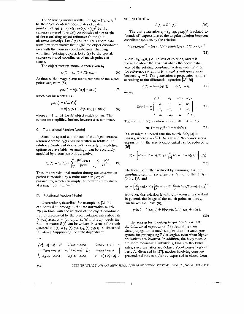
Experimental results for four different cases are reported below. The measurement noise level indicated in each case is the ratio of the standard deviation of the quantization error to that of the signal (expressed as a percentage). The signal standard deviation is defined to be the root-mean-square distance of the feature points from their ccntroid, computed during the frame when the object is farthest from the camera. The initial state estimates mentioned in Cases 1-3 are obtained by a batch procedure; details are provided in a later section and in the Appendix.

The errors in the output estimates of the IEKF in each frame are displayed graphically. It must be noted that the position, structure and translational velocity estimates, and therefore the corresponding errors, are normalized by the (time-varying) z coordinate of the center of the object-centered coordinate system. In the cases discussed, 4 feature points were tracked over 100 frames, and the following parameters were used to generate the motion: w, = wy = U , = 0.2; v, = 0.25; vy = 0.2; v, = 0.15. The object is assumed to be at location (0,0,10) at start. Focal length and sampling period are both assumed to be unity. It is assumed that the feature points have been matched over all the frames. There is no special reason for selecting 4 points, except that it seems unreasonable to expect many more feature point correspondences. In general, the greater the number of matched feature points in each frame, the better will be the performance of the IEKF in terms of speed of convergence and estimation accuracy.

Case I : (Fig. 2) A moderately low measurement noise level of 2.5 percent was used in this case. A crude initial state estimate (with errors of 20 percent or more in some states) was used. As the figures indicate, the position and vclocity estimates converge quite well, requiring about 30 frames for satisfactory convergence. Most of the structure parameters seem to have a small but constant steady-state error, and the attitude parameters (i.e., the quaternions) exhibit sinusoidal oscillations of small magnitude about the correct values. This is probably due to the fact that different combinations of structure and attitude parameters can result in the same spatial position of the feature points, which means that any large errors in the initial structure estimate can cause corresponding errors in the attitude estimates. This problem can be solved by providing more accurate initial structure estimates, or by imposing additional constraints on the structure. Knowledge about the structure of the object

648 IEEE TRANSACTIONS ON AEROSPACE A N D ELECTRONIC SYSTEMS VOL. 26, NO. 4 JULY 1990

-02’ 50 100 -0.1 0 50 100

frame number frame number

I -1 - 50 100 50 IO

-0.2’


50 100 50 100 frame number frame number

Fig. 2. Estimation errors: Case 1. In this and subsequent figures, labels ( x , y , z and 1,2,3,4) are used to indicate vector component

corresponding to each plot.

can also be used for this purpose.

was fairly high (10 percent), and the initial guess was crude as in Case 1. The results are similar to those obtained for Case 1, except that the convergence is slower. For instance, the angular velocities converge in about 50 iterations, compared with 25 iterations required for Case 1. This is mainly due to the higher measurement noise.

The above two experiments demonstrate the basic convergence properties of the IEKF, given an inaccurate initial estimate and noisy observations. In actual practice, a much better initial guess can be obtained, resulting in a greatly improved performance, as shown by the next experiment.

Case 3: (Fig. 4) In this case, the measurement noise was the same as in Case 1, but a much more accurate initial state estimate was used. As the graphs show, the filter “locks on” to the motion almost immediately, and tracks it faithfully. The price we pay for this excellent performance of the IEKF is the greater amount of time spent in getting the (more accurate) initial estimate. All the same, this case is the one of greatest practical interest, since it demonstrates the ability of the IEKF to track the motion effectively given a good initial guess (which can be obtained by a batch algorithm, as described in a later section).

Case 4: (Fig. 5 ) In this case all the initial values of the state vector were set (except the quaternions,

Case 2: (Fig. 3) The measurement noise level here

0 1 -

0

- 0 5 -

0 1

O

-0 1

- O l -

X Y -,

0 - 2 y .

' 2

- -0 1 -

0 1

O

-0 1

- O l -

X Y -,

0 - 2 y .

' 2

- -0 1 -

translational velocit error

-0 05

-0 1 50 100

frame number

I , position error I

o,3 translational velocity error

-01 t I

50 100 - 0 2 '

frame number

0 1

-0.5 U 50 100

frame number

o,2 angular velocity error I

-0.2 50 100

frame number

2 , quatemion error I

05& 0 - - - -

-0.2 - so 100

frame number

-0.6 ' 50 100

frame number -20-+ 100


o,2 structure error: point #4 I

o,6 structure error: point #4

-0 1 Lb-+---l -olol -0.2 50 100

frame number

- 0 4 1 2 , 1 50 100

-0 6

frame number

-0.2 I 50 100

frame number

-04- 50 100

frame number

Fig. 3. Estimation errors: Case 2. Fig. 5. Estimation errors: Case 4.

ol: I translation; y;locity error ~

-0 05

-0 1 50 100

frame number

quatemlon error 1, I

osition error

-0 1

-0 2 50 100

frame number

-0 1

-0 2 50 100

frame number

the performance of the IEKF in the absence of any information about the initial conditions. The velocity and position states of the IEKF, after an initial period of wild fluctuations, converge quite fast, in about 25 iterations. The performance is interesting, considering the extreme nonlinearity of the problem, and the consequent mismodeling produced by linearization. The quaternions, however, do not converge at all, and the structure states seem to converge very slowly. Furthermore, a high degree of instability was observed in the solution, due to ill-conditioning of the matrix to be inverted in the computation of the Kalman gain; its generalized inverse had to be used instead. The performance deteriorated rapidly when small amounts of noise (up to 2.5 percent) were added to the measurements.

I ' I 50 100

frame number

o,2 structure ermr: point #3 o,2 stmcture error. point #4 I I

B. Experiments with Real Imagery

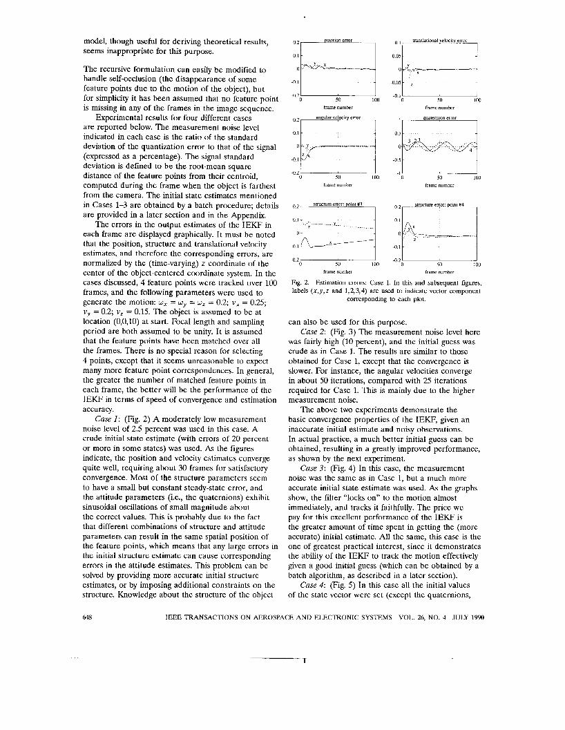
This experiment involves randomly selected points on the side of the tire of a car approaching the camera (Fig. 6) . Seventeen images were made, with eight feature points per frame. The feature points were marked with adhesive dots to facilitate the measurement process. The car was moved approximately 3 in between each frame, corresponding to a tire rotation of about 14.8 deg. The direction of the translation was towards the camera (i.e., in the positive z-direction), with a fairly large component to the right (positive x-direction), and a small downward

-0.2- -0.2' 50 100 50 100


Fig. 4. Estimation errors: Case 3.

which can be trivially initialized if it is assumed that the object-centered and the inertial coordinate systems are aligned at the start of the experiment). Noise-free measurements were used. This case demonstrates


1

Y ’

Fig. 6. First and fourth frames of real image sequence

component due to the positioning of the camera. The object image size (i.e., the size of the tire) is about 2 in at the start of the sequence, and about 3 in at the end. The total rotation was about 4 rad and the total translation about 45 in. The photographs were digitized to a resolution of 50 pixels/in. Two previously chosen reference points were located on all the images, and the distances of the feature points from them were measured on a Sun workstation. A simple geometrical transformation was used to reference all measurements to the coordinate axes in the first image. This was done to reduce errors due to small camera movements during imaging, and the positioning of the photographs during scanning. Feature point correspondences were obtained manually by inspection. The focal length of the imaging system was not known, and was assumed to be unity. This has the effect of scaling the translation and structure parameters up or down, but is not a serious problem since the latter can only be determined up to a scale factor.

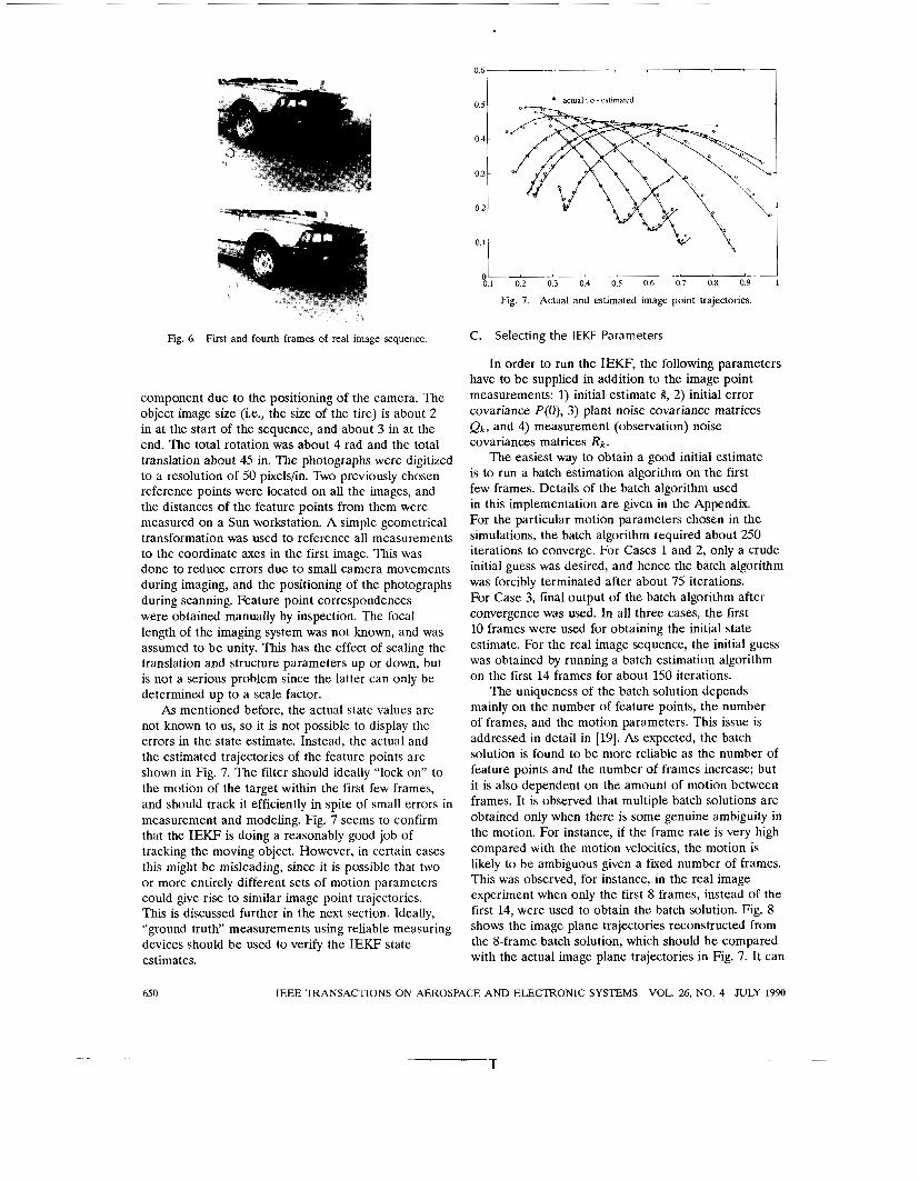
As mentioned before, the actual state values are not known to us, so it is not possible to display the errors in the state estimate. Instead, the actual and the estimated trajectories of the feature points are shown in Fig. 7. The filter should ideally “lock on” to the motion of the target within the first few frames, and should track it efficiently in spite of small errors in measurement and modeling. Fig. 7 seems to confirm that the IEKF is doing a reasonably good job of tracking the moving object. However, in certain cases this might be misleading, since it is possible that two or more entirely different sets of motion parameters could give rise to similar image point trajectories. This is discussed further in the next section. Ideally, “ground truth” measurements using reliable measuring devices should be used to verify the IEKF state estimates.

0.5 -

0.4 -

0.3 -

0.2 ~

0.1 -

* -actual : o - estimated

0.1 0.2 0.3 0.4 0.5 0.6 0.7 0.8 0.9

Fig. 7. Actual and estimated image point trajectories.

C. Selecting the IEKF Parameters

In order to run the IEKF, the following parameters have to be supplied in addition to the image point measurements: 1) initial estimate 9, 2) initial error covariance P(O), 3) plant noise covariance matrices Q k , and 4) measurement (observation) noise covariances matrices Rk.

is to run a batch estimation algorithm on the first few frames. Details of the batch algorithm used in this implementation are given in the Appendix. For the particular motion parameters chosen in the simulations, the batch algorithm required about 250 iterations to converge. For Cases 1 and 2, only a crude initial guess was desired, and hence the batch algorithm was forcibly terminated after about 75 iterations. For Case 3, final output of the batch algorithm after convergence was used. In all three cases, the first 10 frames were used for obtaining the initial state estimate. For the real image sequence, the initial guess was obtained by running a batch estimation algorithm on the first 14 frames for about 150 iterations.

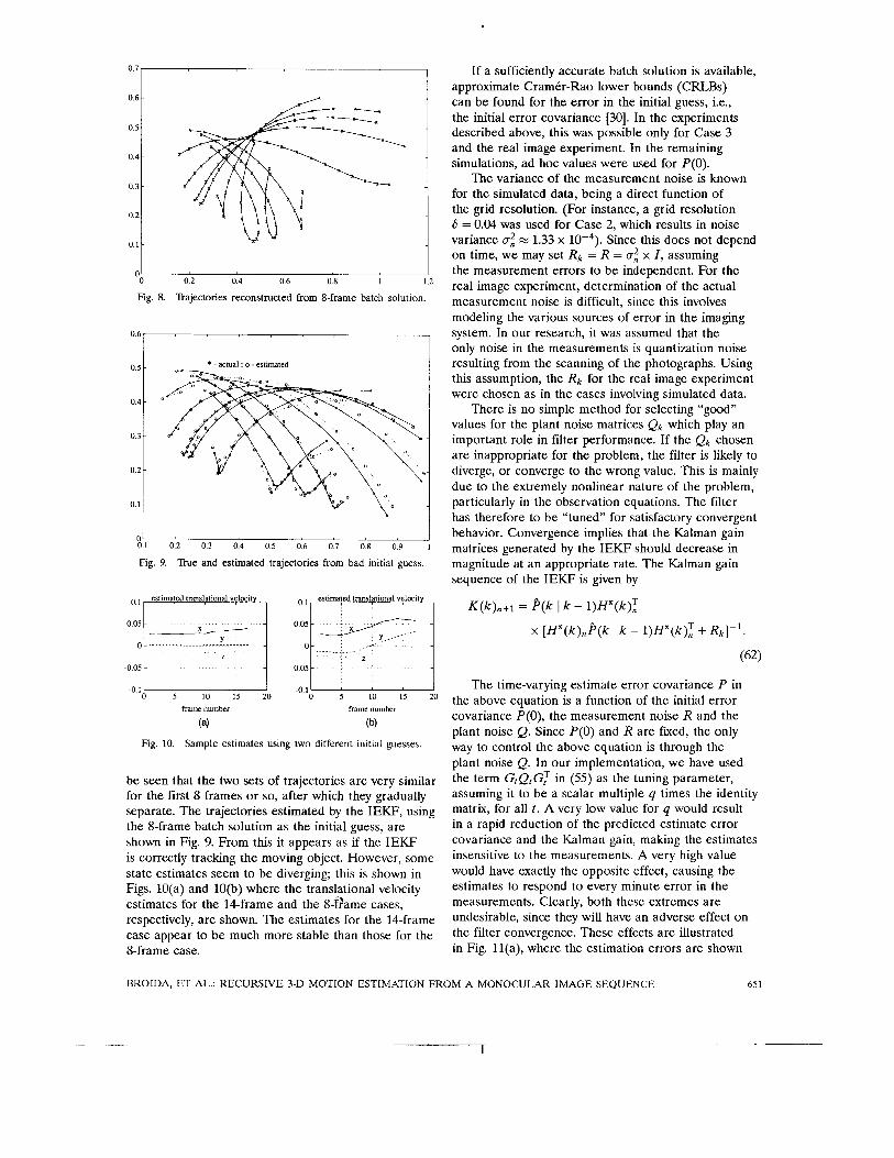
The uniqueness of the batch solution depends mainly on the number of feature points, the number of frames, and the motion parameters. This issue is addressed in detail in [19]. As expected, the batch solution is found to be more reliable as the number of feature points and the number of frames increase; but it is also dependent on the amount of motion between frames. It is observed that multiple batch solutions are obtained only when there is some genuine ambiguity in the motion. For instance, if the frame rate is very high compared with the motion velocities, the motion is likely to be ambiguous given a fixed number of frames. This was observed, for instance, in the real image experiment when only the first 8 frames, instead of the first 14, were used to obtain the batch solution. Fig. 8 shows the image plane trajectories reconstructed from the 8-frame batch solution, which should be compared with the actual image plane trajectories in Fig. 7. It can

The easiest way to obtain a good initial estimate


T

o.6 t 0.4

0.3

0.2

0.5 !-

-

-

-

0.5

0.4-

0.3

0.2

0.1

t

-

’

-

-

-

0 ‘ I

Fig. 8. Trajectories reconstructed from %frame batch solution.

0.2 0.4 0.6 0.8 I 1.2

o ’ 6 / - actual : o - estimated

0 0.1 0.2 0.3 0.4 0.5 0.6 0.7 0.8 0.9 1

Fig. 9. True and estimated trajectories ti-om bad initial guess.

, estimated translational velocit

-0 05 -0 os

-0 1 -0 1 0 5 10 15 20 0 5 10 15 20


(a) (b)

Fig. 10. Sample estimates using two different initial guesses

be seen that the two sets of trajectories are very similar for the first 8 frames or so, after which they gradually separate. The trajectories estimated by the IEKF, using the &frame batch solution as the initial guess, are shown in Fig. 9. From this it appears as if the IEKF is correctly tracking the moving object. However, some state estimates seem to be diverging; this is shown in Figs. lO(a) and lo@) where the translational velocity estimates for the 16frame and the 8-T;ame cases, respectively, are shown. The estimates for the 14-frame case appear to be much more stable than those for the 8-frame case.

If a sufficiently accurate batch solution is available, approximate Cramtr-Rao lower bounds (CRLBs) can be found for the error in the initial guess, i.e., the initial error covariance [30]. In the experiments described above, this was possible only for Case 3 and the real image experiment. In the remaining simulations, ad hoc values were used for P(0).

for the simulated data, being a direct function of the grid resolution. (For instance, a grid resolution 6 = 0.04 was used for Case 2, which results in noise variance U,” M 1.33 x on time, we may set Rk = R = n,” x I , assuming the measurement errors to be independent. For the real image experiment, determination of the actual measurement noise is difficult, since this involves modeling the various sources of error in the imaging system. In our research, it was assumed that the only noise in the measurements is quantization noise resulting from the scanning of the photographs. Using this assumption, the Rk for the real image experiment were chosen as in the cases involving simulated data.

There is no simple method for selecting “good” values for the plant noise matrices Q k which play an important role in filter performance. If the Q k chosen are inappropriate for the problem, the filter is likely to diverge, or converge to the wrong value. This is mainly due to the extremely nonlinear nature of the problem, particularly in the observation equations. The filter has therefore to be “tuned” for satisfactory convergent behavior. Convergence implies that the Kalman gain matrices generated by the IEKF should decrease in magnitude at an appropriate rate. The Kalman gain sequence of the IEKF is given by

The variance of the measurement noise is known

Since this does not depend

K(k),+l = P(k I k - l)H”(k);f

x [ H X ( k ) , p ( k I k - 1)H”(k);f -+Rk] - l .

(62)

The time-varying estimate error covariance P in the above equation is a function of the initial error covariance P(O), the measurement noise R and the plant noise Q. Since P(0) and R are fixed, the only way to control the above equation is through the plant noise Q. In our implementation, we have used the term GtQtG,’ in (55) as the tuning parameter, assuming it to be a scalar multiple q times the identity matrix, for all t . A very low value for q would result in a rapid reduction of the predicted estimate error covariance and the Kalman gain, making the estimates insensitive to the measurements. A very high value would have exactly the opposite effect, causing the estimates to respond to every minute error in the measurements. Clearly, both these extremes are undesirable, since they will have an adverse effect on the filter convergence. These effects are illustrated in Fig. l l (a) , where the estimation errors are shown

BROIDA, ET AL.: RECURSIVE 3-D MOTION ESTIMATION FROM A MONOCULAR IMAGE SEQUENCE 65 1

o5 position error (Case 3) position error (Case 4)

q 2 < q 1 < q 3 e 2 < e l < e 3 05

0 0

i -0.05l " I

50 100 0 50 100


(4 (b) Fig. 11. Effects of varying plant noise ( 4 ) and threshold (e) .

for one state ( X R ) in Case 3 for three different values of q : q1 = our simulations we have chosen, by trial and error, those values of q that have resulted in good filter performance. Several other strategies are possible, involving adaptive estimation, as discussed in [B]. These issues have to be addressed in future work on recursive motion estimation.

Another effect which can be observed in certain rare cases is the ill-conditioning of the matrix inversion involved in (62). The H matrix in the equation is very sparse, and the pre and postmultiplication of P by H and HT, respectively, results in a sparse matrix which has mostly off-diagonal elements, and is therefore likely to be ill-conditioned. The matrix inversion in (62) guaranteed to be well conditioned only if the measurement noise covariance R is sufficiently large (i.e., a large multiple of the unit matrix) and is the dominant term in the matrix summation involved in (62). This condition was not satisfied in Case 4, and the generalized inverse was therefore used. The computation of the generalized inverse of a matrix requires the specification of a threshold parameter ( e ) , below which all singular values of the matrix are set to zero. The effects of varying e on the estimation of one state ( X R ) in Case 4 are shown in Fig. 11@). The estimation errors are plotted for three values of e , O.OOl(el), 0.0001(e2), and O.Ol(e3). The sudden increase in the estimation error near the 5th frame for e = 0.0001 is due to numerical inaccuracies in the computation of the generalized inverse, i.e., ill-conditioning. Higher values of e result in greater numerical stability, but lead to loss of information contained in the smaller singular values. The selection of the threshold could be made automatic by specifying that all singular values falling below a certain fraction of the largest one should be treated as zero. In future work, we will examine other numerically stable approaches such as the square root information filter.

q2 = lo-", and q 3 = 0.1. In

for the kinematics of a rigid object, and for the observation of the discrete features of the object using a single camera. The recursive estimation is done using an IEKF which is initialized by the output of a batch algorithm run on the first few frames.

The recursive estimation technique presented in this paper has numerous advantages over other methods currently in use. First, the recursive nature of the computations makes it suitable for real-time applications like object tracking, automated land vehicle guidance, robot hand-eye coordination, etc. The next major advantage is the flexibility in choosing the number of feature points, and the independence of the algorithms on the number of images in the sequence. The other advantages are robustness in the presence of noise and modeling errors, and ease of implementation. The main drawback with this scheme, as it is with most other feature-based methods, is the need for feature point correspondences; however, the predictive capabilities of the Kalman filter can be used to reduce the computation time required to match the feature points from one frame to the other, as explained in Appendix B. Another drawback is the possibility of filter divergence; this may be overcome by a suitable choice of the initialization parameters, and robust numerical techniques.

The IEKF method of recursive motion/structure estimation can be applied, with suitable modifications, when the image sequence is obtained using two cameras instead of one. The 3-D locations of the feature points can be found using stereo matching, and can be used directly instead of their projections on the image plane [27]. The performance of the IEKF improves considerably if stereo image sequences are used, since the nonlinearity of perspective projection can be eliminated from the measurement equations. Convergence is faster and more reliable, and an accurate initial guess is not required. It is also easier to estimate higher derivatives of the motion parameters. In [27], a constant precession model is used for the rotation of the object, and a constant acceleration model for the translation.

Several other extensions and enhancements to our work are possible. These include use of lines or edges as the features to be tracked (instead of points), interleaving the feature correspondence search with the recursive estimation, and using more general models for the kinematics of the object. Our current research is directed towards accomplishing some of these goals.

APPENDIX A. OBTAINING THE INITIAL ESTIMATE VI. CONCLUSION

In the experiments discussed in this paper, we have used the batch estimation technique developed by Broida and Chellappa, discussed in [22] to obtain the initial state estimates for the IEKE This algorithm does not estimate the quaternions, but the latter

The purpose of this paper is to introduce a recursive method of estimating 3-D kinematics and structure of a rigid moving object from a sequence of noisy monocular images. We have described models


can be trivially initialized if the inertial and the objectcentered coordinate systems are assumed to be aligned initially.

In the batch formulation, the vector U of unknown parameters is

U =

The individual components of s j ( u , t k ) of (6) are (setting to = 0),

Xi(U,tk)

s i (u , t k ) = y i ( u , t k ) 0 zi (U, t k )

i 1 + t k Z / Z R + Rx(u,i,tk) 1 x R / z R + t k i / z R + R x ( u , i , t k )

= Y R / Z R + t k y / z R + R x ( u , i , t k ) .

The terms Rx(u,i,tk), etc., refer to the x - , y-, and z-components of the camera (inertial) coordinates of the ith match point, which are expressed in the rotated (objectcentered) coordinate system as (Xi /ZR,y i /ZR,Zi /ZR) . The rotation matrix R ( u , t k ) of (10) is a function of ~ 6 , u 7 , u ~ ( w x , w y , w ~ ) , and t k . For example, denoting the T S component of R(u,t) as R,,,

R x ( u , i , t k ) = R I I X i / Z R R l 2 Y i / Z R + R13Zi/ZR

= (4; - 4; - 43” + &Xi / zR

+ 2 ( q l q 2 4344)y i /ZR

+ 2(qlq3 - q2q4)z i /zR

where the time argument of q(t) has been suppressed. The 1 in the z-component of Si (U, tk ) is written as ZRjZR, in an analogous manner to the terms u1 = XR/ZR and U2 = Y R / Z R , as discussed above. All

components of the object structure and translational kinematics are then homogeneous in ~ / z R , which accounts for the global scale factor.

Next, the components of (8) are written as

and

Then, if the noise terms n x ( t k ) and n Y ( t k ) are assumed to be independent, identically distributed (IID), zero mean Gaussian, then, finding the maximum likelihood (ML) estimate 0 of U can be shown to be equivalent to minimizing with respect to U the sum of squared residuals:

N M

G(u) = c c { ( x i ( t k ) - h X [S i (u , tk )] )2 k=l i=l

( x ( t k ) - hY[S i (U , t k ) ] )2} - (66)

The above minimization may be done using any standard optimization algorithm. In this research, the IMSL routine for minimization by a quasi-Newton method (UMING) was used. More details of the batch algorithm may be found in [19].

APPENDIX B. OBTAINING FEATURE POINT CORRESPONDENCES

The IEKF described in this paper assumes that the feature points have been matched over successive images (frames) in the sequence. Obtaining feature point matchings is a highly nontrivial problem, and considerable research on this issue has been reported in the literature (for instance, see [31]). This issue has not been addressed in this research, but it appears that in the present formulation the process may be considerably simplified and speeded up by using the predictive capabilities of the Kalman filter. State vectors can be predicted at future time instants, and using these, future feature-point positions in the image sequence can be predicted with known uncertainty. This information can be used to restrict the search space for future matchings.

In order to estimate the image coordinates of a match point at time t , the state estimates S ( t ) must be computed, and then projected directly as h[S(t)].

BROIDA, ET AL.: RECURSIVE 3-D MOTION ESTIMATION FROM A MONOCULAR IMAGE SEQUENCE

----

653

Recall that the state vector is of dimension d and the measurement is of dimension 2M. An approximate error covariance of the resulting image plane location estimates of feature point i is then immediately available as

c(i,t> = ~ ; ( t ) P ( t I D ) H ; ( ~ ) ~ (67)

where H;(t) = V,h[s;(t)] is the 2 x d linearized measurement function, each row corresponding to one of the two image plane coordinates of feature point i, evaluated at the state estimates $(t). Here, P(t I D) is the approximate state covariance matrix at time t , conditioned on all available data (e.g., past and future data, if t represents an interpolation, and past data only if t is an extrapolation). The approximate covariance matrix can be computed by integrating the differential equation (55). In correlating observed feature locations with estimated feature locations, a measure of closeness is desired between the predicted coordinates of feature point i and the measured coordinates of feature point j at time & + I , under the hypothesis that the measured and predicted feature are one and the same. For example, if a single feature is observed, and there are M predicted features, this amounts to an M-ary hypothesis test. As might be expected, the number of hypotheses grows quickly with the number of predicted and observed features, and the possibilities exist that each observed feature could be new (observed for the first time), and/or that each of the predicted features could be occluded. The so-called residual covariance matrix [32] is available by computing the measurement covariance matrix

,

Rj ( t k + l ) = E[v j ( t k + l ) v j ( t k + I ) ~ ] (68)

s i j ( t k + l ) = ~ ; ( k + 1 > P ( t k t 1 I tk)Hi(k + llT + R j ( t k t 1 )

to give the 2 x 2 matrix

(69) making use of (55) and evaluating Hi(k + 1) at G(tk+l) .

The subscript i in H;(k + 1) indicates the 2 x M matrix obtained by taking the gradients of the scalar elements

respect to the state vector s, evaluated at S( tk+ l ) . As discussed in [32], this information can be used to help in associating (labeling) the data observed (unlabeled feature point coordinates) at time t k + l with feature points being tracked, to minimize (or at least estimate) the probability of error in labeling these observed feature points.

Denote the image plane distance 2;; between p; , the predicted coordinates of feature point i , and o;, the coordinates of the observed feature point j , as 2;; = oj - p ; . A normalized distance (xi) can be

x , , k + l = hx[si(tk+l)l and Y i , k + l = hY[Si(lk+l)l with

computed as

If the filter is linear, and the observations are distributed normally, the distances d;j are seen to

d2. = 2?-.s:12.. 1 J 11 1 J '1'

be twice the exponents in the univariate probability density of each observation o; conditioned on the identification of its mean (class label) as E [ p ; ] . Suppose that only a single feature point 01 is observed, and the assumptions of normality hold. Then, the ML estimate of the correct class (the predicted feature point corresponding to the observed point) is given by

i = arg mind;: (71) 1

and the probability of correctly labeling 01 can be computed from the knowledge of the state and measurement covariances, and the normalized distances of the remaining elements { d; l , i = 1, . . . , M } . Next, suppose that M feature points are observed, that they truly represent noisy observations of the existing set of predicted feature points (no extra points, no missing points), and an assignment of measured points to predicted points is desired.

This assignment is computed by observing that the vector of distances {d ; ; ; i , j E T } (where T denotes a particular 1-to-1 assignment of observed feature points j to predicted feature points i ) is multivariate Gaussian. The (unknown) mean vector of this density is the projection of the actual feature points (of which { p i } are estimates) into the image plane; the covariance matrix takes into account the variances of the observations, the estimates, and the process noise. The computation of the probability of error in this process when there are two observations of two features is discusser' in [33].

T that minimizes the sum A solution is obtained by computing the assignment

T = arg mind2 = arg min dTj. T T i , j € T

(72)

An optimal algorithm for this purpose, that identifies the minimum sum correlation even when the number of predicted points is not equal to the number of observed points, is discussed in [32], and is known as Munkres' algorithm, or the Hungarian algorithm. This general approach is well known in operations research problems, and allows the extension of [34] to the recursive case.

REFERENCES

[ l ] Ballard, D. H., and Kimball, 0. A. (1983) Rigid body motion from depth and optical flow. Computer Vision, Graphics and Image Processing, 22 (Apr. 1983), 95-115.

[2] Hildreth, E. C. (1984) Computations underlying the measurement of visual motion. Artificial Intelligence, 23 (Aug. 1984), 309-354.

Determining three-dimensional motion and structure from optical flow generated by several moving objects. IEEE Transactions on Pattern Analysis and Machine Intelligence, PAMI-7 (July 1985), 384-401.

[3] Adiv, G. (1985)


1

Jain, R. C. (1984) Segmentation of frame sequences obtained by a moving observer. IEEE Transactions on Pattem Analysis and Machine Intelligence, PAMI-6 (Sept. 1984), 624.429.

Object tracking with a moving camera. In Proceedings of the IEEE Workshop on Visual Motio?~, Imine, CA, Mar. 1989, 2-12.

Determining the movement of objects from a sequence of images. IEEE Transactions on Pattem Analysis and Machine Intelligence, PAMI-2 (Nov. 1980), 554562.

Estimating three-dimensional motion parameters of a rigid planar patch. IEEE Transactions on Acoustics, Speech, and Signal Processing, ASSP-29 (Dec. 1981), 1147-1152.

Tsai, R. Y., Huang, T. S., and Zhu, W. L. (1982) Estimating three-dimensional motion parameters of a rigid planar patch, 11: Singular value decomposition. IEEE Transactions on Acoustics, Speech, and Signal Processing, ASSP-30 (Aug. 1982), 525-534.

Some experiments on estimating the 3-d motion parameters of a rigid body from two consecutive image frames. IEEE Transactions on Pattern Analysis and Machine Intelligence, PAMI-6 (Sept. 1984), 545-554.

Experiments in estimation of 3-d motion parameters from a sequence of image frames. Presented at the IEEE Conference on Computer Vision and Pattern Recognition, June 1985.

Structure and motion from images: Fact and fiction. In Proceedings of the Third Workshop on Computer Vision: Representation and Control, Oct. 1985, 127-128.

On monocular perception of 3-d moving objects. IEEE Transactions on Pattern Analysis and Machine Intelligence, PAMI-2 (Nov. 1980), 582-583.

Backing known 3-d objects. In Proceedings of National Conference on Artificial Intelligence, August 1982, 1S17.

The motion problem: How to use more than two frames. Technical report IRIS-202, University of Southern California, Institute for Robotics and Intelligent Systems, Los Angeles, CA, Oct. 1986.

Dynamic monocular machine vision. Machine Vision and Applications, 1, 4 (1988).

3-6 motion estimation, understanding, and prediction from noisy image sequence. IEEE Transaciwns on Pattern Analysis and Machine Intelligence, PAMI-9 (May 1987), 370-389.

Stochastic Processes and Filtering Theory. New York Academic Press, 1970.

Broida, T. J., and Chellappa, R. (1986) Kinematics and structure of a rigid object from a sequence of noisy images. In Proceedings of IEEE Workshop on M o t i o ~ Representation and Analysis, May 1986, 95-10,

Burt, P. J., Bergen, J. R., et al. (1989)

Roach, J. W., and Aggamal, J. K. (1980)

Tsai, R. Y., and Huang, T. S. (1981)

Fang, J.-Q., and Huang, T. S. (1984)

Yasumoto, Y., and Medioni, G. (1985)

Aggarwal, J. K., and Mitiche, A. (1985)

Meiri, A. Z. (1980)

Gennery, D. B. (1982)

Shariat, H. (1986)

Dickmanns, E. D., and Graefe, V. (1988)

Weng, J., Huang, T. S., and Ahuja, N. (1987)

Jaminski, A. H. (1970)

Broida, T. J. (1987) Estimating the kinematics and structure of a moving object from a sequence of images. Ph.D. dissertation, University of Southern California, Los Angeles, 1987.

An integrated approach to feature based dynamic vision. In Proceedings of the IEEE Conference on Computer Vision and Pattern Recognition, June 1988, 820-825.

Estimation of object motion parameters from noisy images. IEEE Transactions on Pattern Analysis and Machine Intelligence, PAMI-8, 1 (Jan. 1986), W99.

Kinematics of a rigid object from a sequence of noisy images: a batch approach. In Proceedings of IEEE Conference on Computer Vision and Pattern Recognition, (June 1986), 176-182.

Estimating the kinematics and structure of a moving rigid object from a sequence of noisy monocular images. (submitted for publication).

The use of quaternions with an all-attitude IMU. In Proceedings of the Annual Rocky Mountain Guidance and Control Conference, Jan. 1982, 269-283.

Analysis of strapdown navigation using quaternions. IEEE Transactions on Aerospace and Electronic Systems, AES-14 (Sept. 1978), 764-768.

Spacecraft Attitude Determination and Control. New York D. Reidel Publishing Co., 1978.

3d motion estimation using a sequence of noisy stereo images. In Proceedings of IEEE Conference on Computer Vision and Pattern Recognition, Ann Arbor, MI, June 1988, 710-716.

Stochastic Models, Estimation, and Control, Vol. 2. New York: Academic Press, 1982.

Bar-Itzhack, I. Y., and Oshman, Y. (1985) Attitude determination from vector observations: Quaternion estimation. IEEE Transactions on Aerospace and Electronic Systems, AES-21 (Jan. 1985), 128-135.

Estimation of object motion parameters from noisy images. Journal of the Optical Society of America A, 6, 6 (June 1989), 879889.

Model-Based Feature Matching Using Location. Cambridge, MA: MIT Press, 1984.

Multiple- Target Tracking with Radar Applications. Dedham, MA: Artech House, 1986.

An expression for nearest neighbor data correlation error probability. IEEE Transactions on Aerospace and Electronic Systems; to be published.

Finding trajectories of feature points in a monocular image sequence. IEEE Transactions on Pattern Analysis and Machine Intelligence, ?AMI-9 (Jan. 1987), 56-73.

Dickmanns, E. D. (1988)

Broida, T J., and Chellappa, R. (1986)

Broida, T. J., and Chellappa, R. (1986)

Broida, T. J., and Chellappa, R.

Niva, G. D. (1982)

Friedland, B. (1978)

Wertz, J. R. (Ed.) (1978)

Young, G. S., and Chellappa, R. (1988)

Maybeck, P. S. (1982)

Broida, T. J., and Chellappa, R. (1989)

Baird, H. (1984)

Blackman, S. S. (1986)

Broida, T. J., and Blackman, S. S.

Sethi, I. K., and Jain, R. (1987)


I

Ted J. Broida received the B.A. degree in fine art from Antioch College, Yellow Springs, OH, in 1977, and the B.S., M.S., and Ph.D. degrees in electrical engineering from the University of Southern California, Los Angeles. His doctoral research was performed in the Signal and Image Processing Institute.

He has been employed by Hughes Aircraft Company since 1979, in the Advanced Programs Division of the Radar Systems Group, where he is a Senior Staff Engineer. His work includes design, analysis, and performance prediction of both single sensor and multiple sensor fusion systems for multiple target tracking, as well as real-time sensor and processor resource allocation problems. His research interests also include applications of estimation theory and nonlinear filtering theory. He is the author or coauthor of a number of papers in these areas, co-authored a chapter in Multiple Target Tracking with Radar Applications with S. S. Blackman, and recently presented at a UCLA short course on Tracking with Electro-Optical (Imaging) Sensors.

Dr. Broida was a recipient of the Hughes B.S. Scholarship, and the M.S. and Ph.D. fellowships. In 1980 he was awarded the Certificate of Outstanding Academic Achievement at USC by the Metro LA section of the IEEE.

S. Chandrashekhar (S’SS) received the B.Xch. degree with distinction in electronics from the Regional Engineering College, Calicut, India in 1985, and the M.E. degree with distinction in computer science from the Indian Institute of Science, Bangalore, India in 1987. He is currently working towards a Ph.D. degree in electrical engineering at the University of Southern California, Los Angeles.

especially those related to the analysis of visual motion; use of recursive techniques and neural-like algorithms for computer vision problems; surface reconstruction and stereo.

Mr. Chandrashekhar is a recipient of the Pre-Doctoral Merit Fellowship of the University of Southern California.

He is chiefly interested in current problems in image processing and computer vision,

Rama Chellappa was born in Madras, India, and received the B.S. degree (honors) in electronics and communications engineering from the University of Madras, India, in 1975, and the M.S. degree (with distinction) in electrical communication engineering from the Indian Institute of Science in 1977, and the M.S. and Ph.D. degrees in electrical engineering from Purdue University, West Lafayette, IN, in 1978 and 1981, respectively.

During 1979-1981, he was a Faculty Research Assistant at the Computer Vision Laboratory, University of Maryland, College Park, MD. Since 1986, he has been an Associate Professor in the Electrical Engineering Systems of the University of Southern California, Los Angeles, and as of September 1988, he has been the Director of the Signal aL.1 Image Institute at the University of Southern California, Los Angeles. His current research interest are in Signal and Image Processing, Computer Vision, and Pattern Recognition.

Dr. Chellappa is a member of the Tau Beta Pi and Eta Kappa Nu. He coedited two volumes of selected papers on image analysis and processing, published in Fall 1985. He served as Associate Editor for IEEE Pansactions on Acoustics, Speech and Signal Processing and is a co-editor of Computer Vision, Graplzics and Image Processing: Graphic Models and Imnge Processing. He was a recipient of a National Scholarship from the Government of India during 1%9-1975. He received the 1975 Jawaharlal Nehru Memorial Award from the Department of Education, Government of India, the 1985 Presidential Young Investigator Award, and the 1985 IBM Faculty Development Award. He also received the 1990 School of Engineering Award for Excellence in %aching at the University of Southern California. He was the General Chairman of the 1989 IEEE Computer Society Conference on Computer Vision and Pattern Recognition, IEEE Computer Society Workshop on Artificial Intelligence for Computer Vision and also Program Co-chairman of the NSF sponsored Workshop on Markov Random Fields for Image Processing, Analysis and Computer Vision.


1 -

recursive 3-d motion estimation from a monocular [4, …raghuram/enee731/sfm/00055557.pdf ·...

Documents